Exploiting the hessian for a better convergence of the SCF RDMFT procedure

Abstract

One-body reduced density matrix functional theory (RDMFT) provides an alternative to Density Functional Theory (DFT), able to treat static correlation while keeping a relatively low computation scaling. Its disadvantageous cost comes mainly from a slow convergence of the self-consistent energy optimisation. To improve on that problem, we propose in this work to use the hessian of the energy, including the coupling term. We show that using the exact hessian is very effective in reducing the number of iterations. However, since the exact hessian is too expensive to use in practice, we test different approximations based on an inexpensive exact part and/or BFGS updates.

VU-Amsterdam]Theoretical Chemistry, Faculty of Exact Sciences, VU University, De Boelelaan 1083, 1081 HV Amsterdam, The Netherlands

1 Introduction

Density functional theory (DFT) has been widely used in electronic structure theory over the past few decades because of its advantageous trade-off between cost and accuracy.^{1, 2, 3, 4, 5, 6, 7} However, it can fail already qualitatively, especially for systems with large static correlations.^{8, 9, 10, 11, 12, 13, 14} A promising choice to improve the accuracy in these cases, while keeping a reasonable computation scaling is to use one-body reduced density matrix functional theory (RDMFT), which naturally describes static correlation with fractional occupation numbers. The large cost of the self-consistent field (SCF) minimisation of the ground state energy in RDMFT (SCF-RDMFT) remains, nevertheless, an obstacle to its acceptance by the community,^{15, 16, 17} mostly due to the exceptionally large number of iterations.

RDMFT, similar to DFT, is based on a theorem ^{18, 19, 20} giving the ground state energy as a functional of the one-body reduced density matrix (1-RDM) $\gamma$. The energy then reads

$$E[\gamma]=-\frac{1}{2}\Tr\left\{\Delta\gamma\right\}+\int\gamma(\mathbf{x},\mathbf{x}^{\prime})v_{\text{ext}}(\mathbf{x},\mathbf{x}^{\prime})\mathrm{d}\mathbf{x}\mathrm{d}\mathbf{x}^{\prime}+W[\gamma],$$ (1)

where $\mathbf{x}=\mathbf{r}\sigma$ denotes a combined space-spin coordinate, $v_{\text{ext}}$ is the (non-)local external potential and $W$ the interaction energy functional which needs to be approximated.

Most approximate RDMFT functionals are defined in the basis that diagonalises the 1-RDM,^{21, 22, 23, 24, 25, 26} $\gamma=\sum_{i}n_{i}\ket{\phi_{i}}\bra{\phi_{i}}$, where $n_{i}$ are the (natural) occupation numbers (ONs) and $\phi_{i}$, the natural orbitals (NOs). Therefore, most SCF procedures in RDMFT work directly with the NOs and ONs.^{27, 28, 15, 29} To ensure that the 1-RDM correspond to a physical $N_{e}$-particle ensemble, one has to impose the following, so-called $N$-representability conditions ^{30, 31} : $\sum_{i}n_{i}=N_{e}$ and $0\leq n_{i}\leq 1\;\forall i$. There are several ways to enforce the inequality constraints and in particular parametrization by some suitable function of a variable $x$ with the range $[0,1]$ seems to be a popular choice. One of the earliest parametrizations is the $\cos(x)^{2}$ function,^{18, 32, 33} though the Fermi–Dirac function $1/(\mathrm{e}^{-\beta x}+1)$^{29, 17} and the error function $\erf(x)$³⁴ are perhaps more attractive choices. Other authors opt for more direct optimization with Powell²⁷ or Lagrange multiplier method, in particular also for the constraint on the trace.^{35, 15}

One also has to impose the orthonormality of the NOs. A common way to do so is to write the NOs as a unitary transformation $U$ of an orthonormal basis. The most common form is $U=\exp(X)$, taking $X$ as a real antisymmetric matrix.^{36, 37, 16} Some authors choose to preserve orthonormality only approximately to calculate an optimization step and reothonormalize the NOs afterwards,^{38, 27, 32} brute forcefully apply a Lagrange multiplier method,³⁹ or use an effective Hamiltonian to be diagonalized.^{28, 35, 15, 29, 17}

Virtually all described approaches are based on a two-step scheme in which the ONs and NOs are each optimized in turn. The main disadvantage is that no information of the coupling between the NOs and ONs is used, so typically a large number of macro-iterations is needed to obtain consistency between the NOs and ONs.

A second order single step method which optimizes the NOs and ONs simultaneously seems therefore a sensible direction. The coupling between the NOs and ONs is naturally included via the off-diagonal ON-NO blocks of the hessian in a (quasi-) Newton scheme. An additional reason to use the hessian is that the unitary parametrization of the NOs $U(X)$ yields a non-convex energy functional in terms of the parameters $X$ (even for the exact RDMFT functional). The energy landscape becomes much more bumpy in $X$ parameter space and the NO-NO block of the hessian provides very useful information to guide the optimization algorithm through curved valleys.

The aim of this work is to reduce the total number of iterations required for the SCF procedure to converge to arbitrary precision. To achieve this goal, we identify and address three different issues present in common SCF-RDMFT algorithms. After giving some details on the implementation, in section 2, we first look at the lack of consistency that can arise when optimising the ONs and NOs separately, in section 3. Then we derive the exact hessian and try to extract as much information as possible from it in section 4. Third, we discuss the violation of the secant equation introduced by a common approximation of RDMFT in section 5, and combine it with our second point to obtain an approximation of the hessian in 5.3. We finally conclude in section 6.

2 Numerical details

The purpose of this research being to improve the SCF convergence, we want to avoid as much as possible additional difficulties coming from the functionals themselves. To do so, we have decided to test our methods exclusively on the Müller functional, also known as the Buijse–Baerends (BB) functional,^{40, 41} known for its convexity w.r.t. the 1-RDM.⁴² For the Müller functional

$$W^{\text{MBB}}[\gamma]=\frac{1}{2}\sum_{ij}n_{i}n_{j}[ii|jj]-\frac{1}{2}\sum_{ij}\sqrt{n_{i}n_{j}}[ij|ji],$$ (2)

with

$$[ij|kl]=\int\mathrm{d}\mathbf{r}_{1}\!\!\int\mathrm{d}\mathbf{r}_{2}\frac{\phi_{i}(\mathbf{r}_{1})\phi_{j}(\mathbf{r}_{1})\phi_{k}(\mathbf{r}_{2})\phi_{l}(\mathbf{r}_{2})}{\absolutevalue{\mathbf{r}_{1}-\mathbf{r}_{2}}},$$ (3)

restricting to the spin-summed case, where $0\leq n_{i}\leq 2$, from now on.

As mentioned in the introduction, though the Müller functional is convex w.r.t. the 1RDM, the unitary parametrization $U(X)$ yields a functional which is not convex w.r.t. $X$. Thus the hessian is generally indefinite even for this simple functional (see Fig. 6). It is thus preferable to turn to methods able to handle indefinite hessians, such as trust-region methods. Our implementation is available at https://github.com/NGCartier/SCF-RDMFT_Hess_investigation and uses on the C++ implementation of the fides package,⁴³ relying on an algorithm proposed by Colemann and Li.^{44, 45} This method is expensive because of the use of the eigenvalue decomposition of the hessian. However, a trust-region conjugate-gradient method, which is much more affordable, could be used as a more economical alternative.

In this work, we use the Explicit By Implicit (EBI) method³⁴ to impose the $N$-representability conditions on the ONs. The EBI approach consists in parameterising the ON $n_{i}=\frac{1}{2}\left(\erf(x_{i})\erf(x_{i})+1\right)\;\forall i$, where $x_{i}$ are the variables to optimise and $\mu$ is computed to satisfy the constraint on the trace of the 1-RDM. Since many functionals (including the Müller functional) depend on the square root of the ONs, in order to avoid diverging derivatives for $n_{i}$ going to 0,⁴⁶ we adapt the EBI parametrisation as follows

$$\sqrt{n_{i}}=\frac{1}{\sqrt{2}}\bigl{(}\erf(x_{i}+\mu)+1\bigr{)}.$$ (4)

The NO orthonormality is imposed by a unitary parametrisation via an exponential, as explained in the introduction.

The results are obtained in a cc-pVDZ basis, starting form Hatree–Fock orbitals and a Fermi–Dirac like distribution of the ONs. For the micro-iterations we used the step length, $\norm{s_{k}}$, as termination criterion and for the macro-iterations we used the energy difference w.r.t. the previous iteration, $\absolutevalue{E_{k}-E_{k-1}}$.

3 Consistency between NOs and ONs

It is common in RDMFT to optimise the NOs and ONs successively in two separate steps. The NOs can then be optimised using an iterative diagonalisation approach.^{28, 15} However, if not done carefully, a two-step procedure may lead to a waste of computational time, when the implementation keeps optimising the NOs while they are no longer consistent with the exact ONs (the reciprocal is also true in principle but negligible in practice), as shown by the presence of plateaus in Fig. 1. This means that the approximation of the hessian is not that relevant when using a 2-step optimisation, as it can only improve the micro-iterations, thus here, we used the BFGS approximation (see subsection 5.1 for details) because of its reasonable cost. The easiest way to avoid this unwanted behaviour is to loosen the termination condition on the NO optimisation while keeping a strong termination criterion on the global convergence. This approach can, nonetheless, lead to convergence problems (dark blue lines in Fig. 1), since the loose termination criterion on the NOs is insufficient to reach the tight criterion on the macro-iteration.

This is readily remedied by a dynamic termination condition for the termination threshold $\epsilon_{\text{dyn}}$ of the NO optimisation. The dynamic NO termination criterion $\epsilon_{\text{dyn}}$ would start at a large value and be reduced (for example, after each macro-iteration) to a sufficiently small value to ensure global convergence (green lines in Fig. 1). As simple demonstration we have chosen the update $\epsilon^{(k+1)}=\epsilon^{(k)}/\alpha$. In Fig. 1 we show the energy convergence for $\epsilon^{(0)}=10^{-2}$ and both $\alpha=2$ and $\alpha=3$ in green. Both values for $\alpha$ are very effective in reducing the total amount of iterations compared to the static NO convergence criteria.

Figure 1: Convergence of the energy using different $\epsilon$ criteria for the optimisation of the NO at each macro-iteration, for the H2O molecule. For $\epsilon_{\text{dyn}}$, we start at $\epsilon^{(0)}=10^{-2}$ and take $\epsilon^{(k+1)}=\frac{1}{\alpha}\epsilon^{(k)}$ after each macro-iteration until $\epsilon^{(k)}$ reaches the same precision as the global convergence criterion.

The choice of $\epsilon_{\text{dyn}}$ may, however, be delicate. If we already use an approximate hessian (or even the exact hessian) of the NOs, a more systematic way to include the coupling between NOs and ONs is to use their cross derivatives in the hessian, thus optimising both in a single step (schematized in Fig. 2).

Figure 2: Algorithm of the 2-step procedure in red, modifications to obtain the 1-step version in blue and common part in black.

To show the advantage of the 1-step procedure over the 2-step procedure, we plot the energy convergence for a set of molecules in Fig. 3 and Fig. 4 respectively. We obtain a significant reduction of the total number of iterations (H2O and CH4 molecules). The 1-step algorithm also appears to be overall more robust, as it allows the energy to converge to an error of $10^{-7}$ Hartree for the CH3OH and C2H6 molecules, unlike the 2-step procedure. However, this improvement is not systematic (see the HF molecule). Since the matrix parametrising the NOs, $X$, counts $N(N-1)/2$ degrees of freedom, for a basis of size $N$, the number of entries in the hessian dedicated to NOs is of order $\mathcal{O}(N^{4})$. On the other hand, the number of entries for the coupling between NOs and ONs is of order $\mathcal{O}(N^{3})$ only (we have $N$ variables for the ONs), which means that its cost is asymptotically negligible compared to the hessian of the NOs.

Figure 3: Convergence of the energy using the 2-step procedure with $\epsilon_{\text{dyn}}$ and $\alpha=2$ for different molecules.

Figure 4: Convergence of the energy using a 1-step procedure with hessian approximated by the BFGS method for different molecules.

For a fair comparison, we have tried to keep the implementations as similar as possible, so we have retained the strong macro-condition of the 2-step algorithm in the 1-step one. In principle, this condition should not play any role in the 1-step case as, it acts as a double check by restarting from the converged point. We, nonetheless have observed that this restart of the 1-step optimisation can occasionally save the convergence as it resets the approximation of the hessian, which may have significantly diverged from the exact one.

4 Extracting the cheap part of the exact hessian

4.1 The exact hessian

Expanding the NOs in a given orbital basis $\{\ket{\chi_{i}}\}$ naively as

$$\ket{\phi_{i}}^{(k+1)}=\sum_{j}\ket{\chi_{j}}U_{ji}\bigl{(}Y^{(k+1)}\bigr{)},$$ (5)

(where $Y$ is an anti-symmetric matrix) leads to a very complicated form of the gradient and the hessian, since the derivatives of the unitary matrix $U$ at general $Y$ are very complicated. However, at $Y=0$ the derivatives become quite simple, so instead the expansion is only made about the current iterate

$$\ket{\phi_{i}}^{(k+1)} =\sum_{jp}U_{ij}\bigl{(}X^{(k+1)}\bigr{)}C^{(k)}_{jp}\ket{\chi_{p}},$$ (6)

where $C^{(k)}=U\bigl{(}X^{(k)}\bigr{)}C^{(k-1)}$ and $C^{(0)}=1$. Note that generally $X^{(k+1)}\neq Y^{(k+1)}-Y^{(k)}$, as unitary matrices do not commute. Expanding around the current iterate works directly for an exact energy hessian, $H^{\text{exa}}$, but in the case of an approximate hessian more care is needed (see subsection 5.2). Using Greek indices for the atomic orbital basis and Latin ones for the NO basis, the 1-RDM then attains the form

$$\gamma_{\mu\nu}=\sum_{rst}C_{\mu r}^{T}U_{rs}^{T}n_{s}U_{st}C_{t\nu}.$$ (7)

$U(X)$ can be expanded in a Taylor series for common parameterizations (Cayley ⁴⁷, exponential). For simplicity and consistency with our implementation, we will take the case $U(X)=\exp(X)$, we have $U_{ij}(X)=1+X_{ij}+\frac{1}{2}\sum_{p}X_{ip}X_{pj}+\mathcal{O}\bigl{(}X^{3}\bigr{)}$. The first and second derivatives are then

$$\left.\frac{\partial U_{pq}}{\partial X_{ij}}\right|_{0}={} \delta_{ip}\delta_{jq}-\delta_{iq}\delta_{jp}$$ (8a)

$$\left.\frac{\partial^{2}U_{pq}}{\partial X_{ij}\partial X_{kl}}\right|_{0}={} \frac{1}{2}\bigl{(}\delta_{ip}\delta_{jk}\delta_{lq}-\delta_{ip}\delta_{jl}\delta_{kq}-\delta_{iq}\delta_{jk}\delta_{lq}+\delta_{iq}\delta_{jl}\delta_{kp}$$

$${}-\delta_{ik}\delta_{jp}\delta_{lq}+\delta_{ik}\delta_{jq}\delta_{lp}+\delta_{il}\delta_{jp}\delta_{kq}-\delta_{il}\delta_{jq}\delta_{kp}\bigr{)}.$$ (8b)

Inserting it into (7) we get

$$\left.\frac{\partial\gamma_{\mu\nu}}{\partial X_{ij}}\right|_{0}={} (C^{T}_{\mu j}C_{i\nu}+C^{T}_{\mu i}C_{j\nu})(n_{i}-n_{j})$$ (9a)

$$\left.\frac{\partial^{2}\gamma_{\mu\nu}}{\partial X_{ij}\partial X_{kl}}\right|_{0}={} \delta_{ik}\left(C^{T}_{\mu j}C_{l\nu}+C^{T}_{\mu l}C_{j\nu})(n_{i}-\frac{1}{2}n_{j}-\frac{1}{2}n_{l})\right)$$

$$+\delta_{jl}\left(C^{T}_{\mu i}C_{k\nu}+C^{T}_{\mu k}C_{j\nu})(n_{j}-\frac{1}{2}n_{i}-\frac{1}{2}n_{k}\right)$$

$$-\delta_{il}\left(C^{T}_{\mu j}C_{k\nu}+C^{T}_{\mu k}C_{j\nu})(n_{i}-\frac{1}{2}n_{j}-\frac{1}{2}n_{k}\right)$$

$$-\delta_{jl}\left(C^{T}_{\mu i}C_{l\nu}+C^{T}_{\mu k}C_{i\nu})(n_{j}-\frac{1}{2}n_{i}-\frac{1}{2}n_{l}\right).$$ (9b)

Many 1-RDM functional approximations are only explicitly written in the NO basis because of a dependence $F(n_{i},n_{j})$ on two ONs, which typically do not take the simple form $f(n_{i})g(n_{j})$.^{21, 22, 23, 24, 25, 26} The energy functional then takes the form

$$E[\gamma] =\sum_{\mu\nu}\left(H^{1}_{\mu\nu}\gamma_{\nu\mu}+\frac{1}{2}\sum_{\kappa\lambda}\Bigl{(}\gamma_{\nu\mu}[\mu\nu|\kappa\lambda]\gamma_{\lambda\kappa}+F_{\nu\mu\kappa\lambda}[\mu\lambda|\kappa\nu]\Bigr{)}\right)$$

$$=E_{1}[\gamma]+E_{H}[\gamma]+W_{\boldsymbol{xc}}[\gamma],$$ (10)

where $H^{1}=-\frac{1}{2}\Delta+v_{\text{ext}}$ and $F_{\nu\mu\kappa\lambda}=\sum_{ij}C_{\nu i}^{T}C_{i\mu}F(n_{i},n_{j})C_{\kappa j}^{T}C_{j\lambda}$, the approximated part of the functional. From there, we can derive explicit expressions of the entries of $H^{\text{exa}}$ (see Appendix A).

First, it is interesting to note that the use of $H^{\text{exa}}$ gives a decently fast convergence of the energy. For all the molecules in the test set, an error lower than $10^{-8}$ Hartree is reached within 70 iterations, that is, one or two order(s) of magnitude less than the BFGS approximation (cf. Fig. 4).

Figure 5: Convergence of the energy using $H^{\text{exa}}$ for different molecules.

To verify that the algorithm converged to a minimum, we have computed the eigenvalues of $H^{\text{exa}}$ and checked that they are all non-negative at the end of the convergence. We plot in Fig. 6 the number of negative eigenvalues of the total hessian, as well as of both the ON and the NO blocks separately, for a more detailed analysis. Indeed, the number of negative eigenvalues goes down to zero for all tested molecules. Note that the hessian can initially contain a large number of negative eigenvalues, putting the emphasis on the nonconvexity of our problem even for the Müller functional. Moreover, most of the negative eigenvalues come from the NO block of the hessian (lines denoted by $\times$), indicating that the hardest part to handle numerically is the optimisation of the NOs.

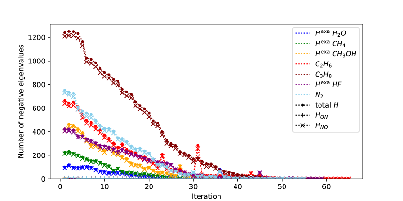
Figure 6: Number of negative eigenvalues of the full $H^{\text{exa}}$ denoted with $\bullet$, of the ON block denoted with $+$ and of the NO block of $H^{\text{exa}}$ denoted with $\times$ for different molecules.

Unfortunately, the excessive cost to compute $H^{\text{exa}}$ of $\mathcal{O}(N^{5})$ makes its use for practical calculations not a viable option. Therefore, we aim for an efficient approximation that retains as much of $H^{\text{exa}}$ as possible.

4.2 The cheap part of the hessian

For functionals of the form $F(n_{i},n_{j})=f(n_{i})f(n_{j})$, sometimes called separable functionals, we can use the idea proposed by Giesbertz⁴⁸ to reduce the scaling of the contribution to $H^{\text{exa}}$ from the first term of (33), first two terms of (36) and the first four lines of (40), from $\mathcal{O}(N^{5})$ to $\mathcal{O}(N^{4})$ (see Fig. 7). Indeed, denoting $v^{K}_{ij}=\sum_{p}f(n_{p})[ip|jp]$, (33), (36) and (40) become

$$\left.\frac{\partial^{2}W_{\boldsymbol{xc}}}{\partial x_{i}\partial x_{j}}\right|_{0}=\sum_{k}\left(\frac{\partial^{2}f(n_{k})}{\partial x_{i}\partial x_{j}}v^{K}_{kk}+\frac{\partial f(n_{k})}{\partial x_{i}}\frac{\partial v^{K}_{kk}}{\partial x_{j}}\right),$$ (11)

$$\left.\frac{\partial^{2}W_{\boldsymbol{xc}}}{\partial X_{ij}\partial x_{k}}\right|_{0}=2\left(\frac{\partial f_{i}}{\partial x_{k}}v^{K}_{ij}-\frac{\partial f_{j}}{\partial x_{k}}v^{K}_{ji}+f_{i}\frac{\partial v^{K}_{ij}}{\partial x_{k}}-f_{j}\frac{\partial v^{K}_{ji}}{\partial x_{k}}\right).$$ (12)

and

$$\begin{split}\left.\frac{\partial^{2}W_{\boldsymbol{xc}}}{\partial X_{ij}\partial X_{pq}}\right|_{0}&=2\delta_{pi}v^{K}_{qj}(2f(n_{i})-f(n_{j})-f(n_{q}))+2\delta_{qj}v^{K}_{ip}(2f(n_{j})-f(n_{i})-f(n_{p}))\\ &-2\delta_{iq}v^{K}_{jp}(2f(n_{i})-f(n_{j})-f(n_{p}))-2\delta_{jp}v^{K}_{iq}(2f(n_{j})-f(n_{i})-f(n_{q}))\\ &+4(f(n_{i})f(n_{p})-f(n_{j})f(n_{p})-f(n_{i})f(n_{q})+f(n_{j})f(n_{q}))[ip|jq].\end{split}$$ (13)

We can analogously compute the corresponding terms of (32), (35) and (39) in $\mathcal{O}(N^{4})$, by computing separately $v^{J}_{ij}=\sum_{p}f(n_{p})[ij|pp]$. Moreover, the one-electron part of $H^{\text{exa}}$ can clearly be obtained in $\mathcal{O}(N^{4})$ [even only $\mathcal{O}(N^{3})$].

For the following expressions, we use uppercase for indices going from $N+1$ to $N(N+1)/2$, which can more conveniently be mapped to two indices (the first one going from $1$ to $N$ and the second one being strictly lower than the first one). We denote $H^{\exp}$ such that

$$H^{\exp}_{ij}={} \sum_{k}\left(\frac{\partial f(n_{k})}{\partial x_{i}}\frac{\partial v^{J}_{kk}}{\partial x_{j}}-\frac{\partial f(n_{k})}{\partial x_{i}}\frac{\partial v^{K}_{kk}}{\partial x_{j}}\right)$$ (14a)

for the ON block,

$$H^{\exp}_{Ik}={} H^{\exp}_{ijk}=2\left(f(n_{i})\frac{\partial v^{J}_{ij}}{\partial x_{k}}-f(n_{j})\frac{\partial v^{J}_{ji}}{\partial x_{k}}-f(n_{i})\frac{\partial v^{K}_{ij}}{\partial x_{k}}+f(n_{j})\frac{\partial v^{K}_{ji}}{\partial x_{k}}\right)$$ (14b)

for the coupling block and

$$H^{\exp}_{IP}={} H^{\exp}_{ijpq}=4(n_{i}n_{p}-n_{j}n_{p}-n_{i}n_{q}+n_{j}n_{q})[ij|pq]$$

$${}+4(f(n_{i})f(n_{p})-f(n_{j})f(n_{p})-f(n_{i})f(n_{q})+f(n_{j})f(n_{q}))[ip|jq]$$ (14c)

for the NO block and $H^{\text{cheap}}=H^{\text{exa}}-H^{\exp}$. The scaling to obtain $H^{\text{cheap}}$ is then $\mathcal{O}(N^{4})$ for a separable functional (that is, the same as to obtain the gradient), and we want to approximate $H^{\exp}$ only.

To do so, we can first neglect $H^{\exp}$ entirely and take $B=H^{\text{cheap}}$ as an hessian approximation. (We use $B$ to denote an approximation to the hessian.) We tried it for our set of molecules in Fig. 8 and observed a good convergence for the first few tens of iterations. This approximation can even accidentally outperform the exact hessian (see the H2O molecule in Fig. 9). However, this is a very crude approximation and the algorithm cannot converge for half of the molecules. This seems to indicate that $H^{\text{cheap}}$ provides a good approximation of $H^{\text{exa}}$ for the first few iterations which is sufficient to make H2O, CH4 and HF converge up to $10^{-8}$ Hartree but only $10^{-2}$ for N2 and C2H6.

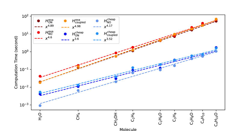
Figure 7: Computation time to obtain the different blocks of the hessian (dotted lines) for $H^{\text{exa}}$ (red lines) and $H^{\text{cheap}}$ (blue lines) w.r.t. the size of different molecules. Asymptotic behaviours are fitted (dashed lines), the formal scaling is $\mathcal{O}(N^{5})$ for $H^{\text{exa}}$ and $\mathcal{O}(N^{4})$ for $H^{\text{cheap}}$.

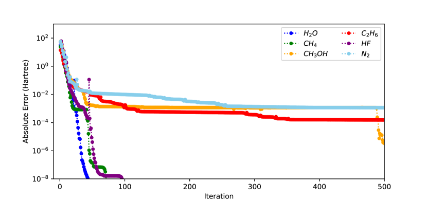
Figure 8: Convergence of the energy using $B=H^{\text{cheap}}$ for different molecules.

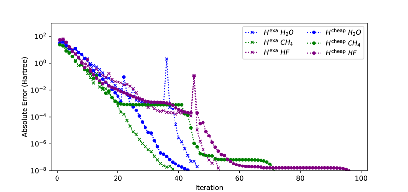
Figure 9: Comparison of the convergence of the energy using $B=H^{\text{cheap}}$, denoted by $\bullet$ and $B=H^{\text{exa}}$, denoted by $\times$ for different molecules.

To assess this assumption, we looked at the error made by taking $B=H^{\text{cheap}}$ in Fig. 10 for the different blocks of the hessian. This shows that the ON block of the hessian is decently approximated by $H^{\text{cheap}}$ while the off-diagonal elements of the NO block and the coupling block are less accurate. The pattern of the upper panels of Fig. 10 shows that the error in the NO block remains low when two indices of $X_{ij}$ and $X_{pq}$ are equal, that is, when $H^{\text{cheap}}_{ijpq}\neq 0$, highlighting the use of $H^{\text{cheap}}$.

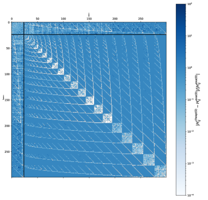
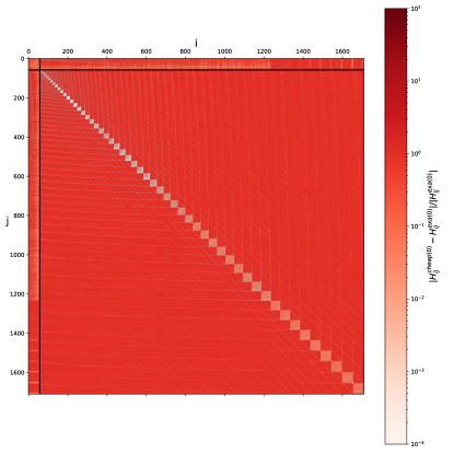
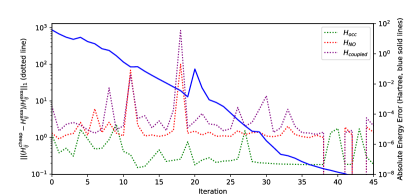
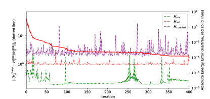
Figure 10: Relative error of $H^{\text{cheap}}$ in the first iteration $\absolutevalue{\frac{H^{\text{cheap}(0)}_{ij}-H^{\text{exa}(0)}_{ij}}{H^{\text{exa}(0)}_{ij}}}$ (top panels), the black lines indicate the separation between the different blocks of the hessian. And norm of that relative error along the optimisation $\norm{\frac{H^{\text{cheap}}_{ij}-H^{\text{exa}}_{ij}}{H^{\text{exa}}_{ij}}}_{1}$ divided by the number of entries of the hessian block (dotted lines in bottom panels) for the ON block (green lines), NO block (red lines) and coupling block (purple lines). Results are shown for the H2O (left panels) and C2H6 molecule (right panels).

To avoid convergence issues for most systems, we thus need a suitable approximation of $H^{\exp}$ and will propose two in subsections 5.3.

5 Approximate hessians

5.1 The BFGS approximation

The most common numerical approximation of the hessian in the literature is the BFGS approximation.⁴⁹ The BFGS update is obtained by demanding that the new approximate hessian $B$ is close to the previous one $B^{(k)}$ under the constraints that the new approximate is symmetric and that $B$ satisfies the secant equation⁴⁹. That is, the BFGS update solves

$$\min_{B\in\mathds{R}^{N\times N}}\norm{B-B^{(k)}}\quad\text{ s.t. }\quad B^{T}=B\text{ and }Bs^{(k)}=y^{(k)},$$ (15)

where $s^{(k)}$ and $y^{(k)}$ the step and difference of the gradient between the $(k+1)^{th}$ and $k^{th}$ iterations respectively. The constraint $Bs^{(k)}=y^{(k)}$ is the secant equation, which simply means that the hessian corresponds to a quadratic model through the last two iterates. Using the Frobenius norm, we obtain the standard BFGS update (see Appendix B for details)

$$B^{(k+1)}=B^{(k)}-\frac{B^{(k)}s^{(k)}s^{(k)T}B^{(k)}}{s^{(k)T}B^{(k)}s^{(k)}}+\frac{y^{(k)}y^{(k)T}}{s^{(k)T}y^{(k)}},$$ (16)

The error induced by the BFGS approximation is actually large, as can be seen from Fig. 11, where we plotted the error made by the BFGS approximation compared to the exact hessian. Since the BFGS approximation encourages a positive hessian it has a hard time reproducing correctly the exact hessian (which is indefinite, see Fig. 6) for the first few iterations, but is supposed to reduce the error while getting closer to the minimum. However, we observe that this is not the case, indicating that the BFGS approximation may not suffice to efficiently approximate the exact hessian.

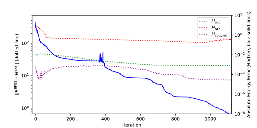
Figure 11: Error of the BFGS approximation $\|B^{\text{BFGS}}-H^{\text{exa}}\rVert$ (dotted line) for the H2O molecule (top) and CH3OH molecule (bottom). The error coming from the ON block is plotted as dotted red lines, from the NO block as green lines and from the coupling blocks as purple lines.

5.2 The BFGS approximation in different spaces

Due to the parametrization, the vector w.r.t. which we actually minimise the energy is $\boldsymbol{x}=(x,X^{\text{up}})$ ($X^{\text{up}}$, vector of the strictly upper triangle entries of $X$), defining what we will call the $\boldsymbol{x}$-space. On the other hand, we will call the $\boldsymbol{\nu}$-space (‘NU-space’), the space where the energy derivatives can be directly calculated, i.e. $\boldsymbol{\nu}=(\sqrt{n},U)$, where $U$ comprises all entries of the full $N\times N$ matrix. We can readily transform the relevant derivatives from the $\boldsymbol{\nu}$- to the $\boldsymbol{x}$-space using the Jacobian matrix $J_{pq}=\frac{\partial\boldsymbol{\nu}_{p}}{\partial\boldsymbol{x}_{q}}$ and its derivative. The BFGS approximation as introduced before (Sec. 5.1 and Sec. 3) was directly applied to the hessian in $\boldsymbol{x}$-space. However, the hessian tends to have a nicer expression in $\boldsymbol{\nu}$-space (is often quartic in $U$ and the square roots of ONs). Also the fact that the unitary parametrization tends to make the hessian indefinite points to a different strategy to use the BFGS update on the hessian in $\boldsymbol{\nu}$-space.

Denoting $\gradient_{\boldsymbol{\nu}}$ the gradient in $\boldsymbol{\nu}$-space, $\gradient^{2}_{\boldsymbol{x}}$ the hessian operator in $\boldsymbol{x}$-space, the energy hessians in $\boldsymbol{x}$- and $\boldsymbol{\nu}$-space are related by the chain rule as

$$H_{\boldsymbol{x}}=J^{T}H_{\boldsymbol{\nu}}J+\gradient_{\boldsymbol{\nu}}^{T}E\,\gradient^{2}_{\boldsymbol{x}}\boldsymbol{\nu}.$$ (17)

Now we have several choices to define closeness to the previous approximation. One option is to make the update close to the previous hessian with updated Jacobian terms

$$\tilde{B}_{\boldsymbol{x}}^{(k)}=J^{(k+1)T}B_{\boldsymbol{\nu}}^{(k)}J^{(k+1)}+\gradient^{T}_{\boldsymbol{\nu}}E|_{(k+1)}\gradient^{2}_{\boldsymbol{x}}\boldsymbol{\nu}^{(k+1)}.$$ (18)

The BFGS optimization problem now becomes

$$\min_{B}\norm\big{B-\tilde{B}_{\boldsymbol{x}}^{(k)}}\quad\text{s.t.}\quad\text{$B^{T}=B$ and $Bs_{\boldsymbol{x}}^{(k)}=y_{\boldsymbol{x}}^{(k)}$},$$ (19)

where $s_{\boldsymbol{x}}^{(k)}$, $y_{\boldsymbol{x}}^{(k)}$ are the step and difference of gradient between the $(k+1)^{th}$ and $k^{th}$ iterations in $\boldsymbol{x}$-space. So we simply need to set $y^{(k)}\to y_{\boldsymbol{x}}^{(k)}$, $B^{(k)}\to\tilde{B}_{\boldsymbol{x}}^{(k)}$ and $s^{(k)}\to s_{\boldsymbol{x}}^{(k)}$, which yields the update

$$B_{\boldsymbol{x}}^{(k+1)} =\tilde{B}_{\boldsymbol{x}}^{(k)}-\frac{\tilde{B}_{\boldsymbol{x}}^{(k)}s_{\boldsymbol{x}}^{(k)}s_{\boldsymbol{x}}^{(k)T}\tilde{B}_{\boldsymbol{x}}^{(k)}}{s_{\boldsymbol{x}}^{(k)T}\tilde{B}_{\boldsymbol{x}}^{(k)}s_{\boldsymbol{x}}^{(k)}}+\frac{y_{\boldsymbol{x}}^{(k)}y^{(k)T}_{\boldsymbol{x}}}{y^{(k)T}_{\boldsymbol{x}}s^{(k)}_{\boldsymbol{x}}},$$ (20a)

which can be transformed to the update in $$\boldsymbol{\nu}$$-space via (17)

$$B_{\boldsymbol{\nu}}^{(k+1)} =B_{\boldsymbol{\nu}}^{(k)}-\frac{\bigl{(}B_{\boldsymbol{\nu}}^{(k)}\bar{s}^{(k)}_{\boldsymbol{\nu}}+\bar{\rho}^{(k)}_{\boldsymbol{\nu}}\bigr{)}\bigl{(}B_{\boldsymbol{\nu}}^{(k)}\bar{s}^{(k)}_{\boldsymbol{\nu}}+\bar{\rho}^{(k)}_{\boldsymbol{\nu}}\bigr{)}^{T}}{\bar{s}^{(k)T}_{\boldsymbol{\nu}}\bigl{(}B_{\boldsymbol{\nu}}^{(k)}\bar{s}^{(k)}_{\boldsymbol{\nu}}+\bar{\rho}^{(k)}_{\boldsymbol{\nu}}\bigr{)}}+\frac{\bar{y}^{(k)}_{\boldsymbol{\nu}}\bar{y}^{(k)T}_{\boldsymbol{\nu}}}{\bar{y}^{(k)T}_{\boldsymbol{\nu}}\bar{s}^{(k)}_{\boldsymbol{\nu}}}$$ (20b)

where

$$\bar{s}^{(k)}_{\boldsymbol{\nu}} \coloneqq J^{(k+1)}s_{\boldsymbol{x}}^{(k)}, \bar{y}^{(k)}_{\boldsymbol{\nu}} \coloneqq J^{(k+1)-T}y_{\boldsymbol{x}}^{(k)}, \bar{\rho}^{(k)}_{\boldsymbol{\nu}} \coloneqq J^{(k+1)-T}\gradient^{T}_{\boldsymbol{\nu}}E|_{(k+1)}\gradient^{2}_{\boldsymbol{x}}\boldsymbol{\nu}^{(k+1)}s^{(k)}_{\boldsymbol{x}}.$$ (21)

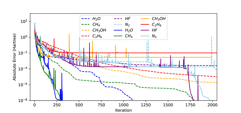
Figure 12: Convergence of the energy using equation (20) in solid lines and (16) in dashed lines for different molecules.

The improvement w.r.t. the BFGS in $\boldsymbol{x}$-space (dashed lines) is significant for most molecules of the test set (see Fig. 12), but the algorithm shows difficulties to converge for the HF, CH3OH and C2H6 molecules. Indeed, it spends hundreds of iterations at an error of $2\cdot 10^{-4}$ Hartree before resuming the convergence for the HF molecule (purple line) and simply stops without finding the correct minimum for the other two molecules.

An other sensible option is to make the hessians close in $\boldsymbol{\nu}$-space, whilst still demanding the secant equation in $\boldsymbol{x}$-space, so

$$\min_{B}\norm\big{B-B_{\boldsymbol{\nu}}^{(k)}}\quad\text{s.t. \quad$B^{T}=B$ and $B\bar{s}^{(k)}_{\boldsymbol{\nu}}=\bar{y}^{(k)}_{\boldsymbol{\nu}}-\bar{\rho}^{(k)}_{\boldsymbol{\nu}}$}.$$ (22)

So we simply need to set $y^{(k)}\to\bar{y}^{(k)}_{\boldsymbol{\nu}}-\bar{\rho}^{(k)}_{\boldsymbol{\nu}}$, $B^{(k)}\to B_{\boldsymbol{\nu}}^{(k)}$ and $s^{(k)}\to\bar{s}^{(k)}_{\boldsymbol{\nu}}$, which yields

$$B^{(k+1)}_{\boldsymbol{\nu}} =B^{(k)}_{\boldsymbol{\nu}}-\frac{B^{(k)}_{\boldsymbol{\nu}}\bar{s}_{\boldsymbol{\nu}}^{(k)}\bar{s}_{\boldsymbol{\nu}}^{(k)T}B^{(k)}_{\boldsymbol{\nu}}}{\bar{s}_{\boldsymbol{\nu}}^{(k)T}B^{(k)}_{\boldsymbol{\nu}}\bar{s}_{\boldsymbol{\nu}}^{(k)}}+\frac{\bigl{(}\bar{y}^{(k)}_{\boldsymbol{\nu}}-\bar{\rho}^{(k)}_{\boldsymbol{\nu}})\bigl{(}\bar{y}^{(k)}_{\boldsymbol{\nu}}-\bar{\rho}^{(k)}_{\boldsymbol{\nu}}\bigr{)}^{T}}{\bar{s}_{\boldsymbol{\nu}}^{(k)T}\bigl{(}\bar{y}^{(k)}_{\boldsymbol{\nu}}-\bar{\rho}^{(k)}_{\boldsymbol{\nu}}\bigr{)}},$$ (23a)

which transformed to $$\boldsymbol{x}$$-space via (17) becomes

$$B^{(k+1)}_{\boldsymbol{x}} =\tilde{B}^{(k)}_{\boldsymbol{x}}-\frac{\bar{B}^{(k)}_{\boldsymbol{x}}s_{\boldsymbol{x}}^{(k)}s_{\boldsymbol{x}}^{(k)T}\bar{B}^{(k)}_{\boldsymbol{x}}}{s_{\boldsymbol{x}}^{(k)T}\bar{B}^{(k)}_{\boldsymbol{x}}s_{\boldsymbol{x}}^{(k)}}+\frac{\bigl{(}y_{\boldsymbol{x}}^{(k)}-\rho^{(k)}_{\boldsymbol{x}}\bigr{)}\bigl{(}y_{\boldsymbol{x}}^{(k)}-\rho^{(k)}_{\boldsymbol{x}}\bigr{)}^{T}}{s_{\boldsymbol{x}}^{(k)T}\bigl{(}y_{\boldsymbol{x}}^{(k)}-\rho^{(k)}_{\boldsymbol{x}}\bigr{)}}$$ (23b)

where $\rho^{(k)}_{\boldsymbol{x}}\coloneqq J^{(k+1)T}\bar{\rho}^{(k)}_{\boldsymbol{\nu}}=\gradient^{T}_{\boldsymbol{\nu}}E|_{(k+1)}\gradient^{2}_{\boldsymbol{x}}\boldsymbol{\nu}^{(k+1)}s^{(k)}_{\boldsymbol{x}}$ and $\bar{B}^{(k)}_{\boldsymbol{x}}=J^{(k+1)T}B^{(k)}_{\boldsymbol{\nu}}J^{(k+1)}$. However, this approximation performed worse than the previous one in preliminary results and was not further tested.

It needs to be mentioned that we have not implemented the gradient difference in the updates (20) and (23) exactly and neither in the BFGS update from section 3, since it reads in full

$$y_{\boldsymbol{x}}^{(k)}=J^{(k+1)}(0)\gradient_{\boldsymbol{\nu}}E\bigr{\rvert}_{(k+1)}-J^{(k+1)}\bigl{(}-s_{\boldsymbol{x}}^{(k)}\bigr{)}\gradient_{\boldsymbol{\nu}}E\bigr{\rvert}_{(k)}.$$ (24)

The Jacobian is very tough to evaluate for the exponential parametrization for $X\neq 0$. As a pragmatic solution, assuming that the step is small enough, we have only taken the zeroth order term from its Taylor expansion for the part parametrizing the NOs

$$J^{(k+1)}(-\{s_{ON\boldsymbol{x}}^{(k)},s_{NO\boldsymbol{x}}^{(k)}\})\approx J^{(k+1)}(-\{s_{ON\boldsymbol{x}}^{(k)},0\}),$$ (25)

which we will call the $0^{th}$ order approximation.

This problem can actually be avoided by applying the BFGS procedure in the $\boldsymbol{\nu}$-space. The BFGS update in $\boldsymbol{\nu}$-space is obtained by simply putting the $\boldsymbol{\nu}$-space quantities into (16), which yields

$$B^{(k+1)}_{\boldsymbol{\nu}} =B^{(k)}_{\boldsymbol{\nu}}-\frac{B^{(k)}_{\boldsymbol{\nu}}s_{\boldsymbol{\nu}}^{(k)}s_{\boldsymbol{\nu}}^{(k)T}B^{(k)}_{\boldsymbol{\nu}}}{s_{\boldsymbol{\nu}}^{(k)T}B^{(k)}_{\boldsymbol{\nu}}s_{\boldsymbol{\nu}}^{(k)}}+\frac{y_{\boldsymbol{\nu}}^{(k)}y_{\boldsymbol{\nu}}^{(k)T}}{s_{\boldsymbol{\nu}}^{(k)T}y_{\boldsymbol{\nu}}^{(k)}},$$ (26a)

which is the transformed to $$\boldsymbol{x}$$-space via (17) to

$$B^{(k+1)}_{\boldsymbol{x}} =\tilde{B}^{(k)}_{\boldsymbol{x}}-\frac{\bar{B}^{(k)}_{\boldsymbol{\nu}}\bar{s}^{(k)}_{\boldsymbol{x}}\bar{s}^{(k)T}_{\boldsymbol{x}}\bar{B}^{(k)}_{\boldsymbol{\nu}}}{\bar{s}^{(k)T}_{\boldsymbol{x}}\bar{B}^{(k)}_{\boldsymbol{\nu}}\bar{s}^{(k)}_{\boldsymbol{x}}}+\frac{\bar{y}^{(k)}_{\boldsymbol{x}}\bar{y}^{(k)T}_{\boldsymbol{x}}}{\bar{s}^{(k)T}_{\boldsymbol{x}}\bar{y}^{(k)}_{\boldsymbol{x}}},$$ (26b)

where $\bar{s}^{(k)}_{\boldsymbol{x}}\coloneqq J^{(k+1)-1}s_{\boldsymbol{\nu}}^{(k)}$ and $\bar{y}^{(k)}_{\boldsymbol{x}}\coloneqq J^{(k+1)}y_{\boldsymbol{\nu}}^{(k)}$.

Though this update could be implemented without additional approximations, the BFGS update in the $\boldsymbol{\nu}$-space actually leads to more convergence problems than (20) as we demonstrate in Fig. 13. We suspect that the issue here is that the secant equation in $\boldsymbol{\nu}$-space is less relevant than the secant equation in $\boldsymbol{x}$-space, as we aim to make a quadratic model in $\boldsymbol{x}$ space.

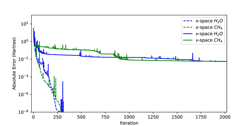
Figure 13: Convergence of the energy using equation (26) in solid lines and (20) in dashed lines for the H2O and CH4 molecules.

5.3 Approximating $B^{\exp}$ with BFGS

As BFGS seems not being very capable of approximating the full hessian sufficiently, we can use the fact that a significant part of the hessian could be calculated in a reasonable computational time: $H^{\text{cheap}}$ (see subsection 4.2). So instead we can ask BFGS to approximate on the expensive part of the hessian $B^{\exp}_{\boldsymbol{\nu}}\approx H^{\exp}_{\boldsymbol{\nu}}$ for us.

Making the updated hessian close to the previous hessian with updated Jacobian terms and $H^{\text{cheap}}$

$$\tilde{B}_{\boldsymbol{x}}^{\exp(k)}\coloneqq J^{(k+1)T}B_{\boldsymbol{\nu}}^{\exp(k)}J^{(k+1)}+H^{\text{cheap}(k+1)}_{\boldsymbol{x}}$$ (27)

means simply replacing $\tilde{B}_{\boldsymbol{x}}^{(k)}\to\tilde{B}_{\boldsymbol{x}}^{\exp(k)}$ in (19), so we get the update

$$B_{\boldsymbol{\nu}}^{\exp(k+1)} =B_{\boldsymbol{\nu}}^{\exp(k)}-\frac{\bigl{(}B_{\boldsymbol{\nu}}^{\exp(k)}\bar{s}^{(k)}_{\boldsymbol{\nu}}+\bar{\xi}^{(k)}_{\boldsymbol{\nu}}\bigr{)}\bigl{(}B_{\boldsymbol{\nu}}^{\exp(k)}\bar{s}^{(k)}_{\boldsymbol{\nu}}+\bar{\xi}^{(k)}_{\boldsymbol{\nu}}\bigr{)}^{T}}{\bar{s}^{(k)T}_{\boldsymbol{\nu}}\bigl{(}B_{\boldsymbol{\nu}}^{\exp(k)}\bar{s}^{(k)}_{\boldsymbol{\nu}}+\bar{\xi}^{(k)}_{\boldsymbol{\nu}}\bigr{)}}+\frac{\bar{y}^{(k)}_{\boldsymbol{\nu}}\bar{y}^{(k)T}_{\boldsymbol{\nu}}}{\bar{y}^{(k)T}_{\boldsymbol{\nu}}\bar{s}^{(k)}_{\boldsymbol{\nu}}},$$ (28)

where

$$\bar{\xi}_{\boldsymbol{\nu}}^{(k)} \coloneqq J^{(k+1)-T}H^{\text{cheap}(k+1)}_{\boldsymbol{x}}s_{\boldsymbol{x}}^{(k)}=H^{\text{cheap}(k+1)}_{\boldsymbol{\nu}}\bar{s}_{\boldsymbol{\nu}}^{(k)}+\bar{\rho}_{\boldsymbol{\nu}}^{(k)}.$$ (29)

Note that $H^{\text{cheap}}$ plays a similar role as the $\gradient_{\boldsymbol{\nu}}^{T}E\,\gradient^{2}_{\boldsymbol{x}}\boldsymbol{\nu}$ term, so lead to the simple replacement $\bar{\rho}_{\boldsymbol{\nu}}^{(k)}\to\bar{\xi}_{\boldsymbol{\nu}}^{(k)}$ between (20b) and (28).

Demanding closeness to the expensive part in $\boldsymbol{\nu}$-space is identical to the update (23a) with $B^{(k)}_{\boldsymbol{\nu}}\to B^{\exp(k)}_{\boldsymbol{\nu}}$ and $\bar{\rho}_{\boldsymbol{\nu}}^{(k)}\to\bar{\xi}_{\boldsymbol{\nu}}^{(k)}$

$$B^{\exp(k+1)}_{\boldsymbol{\nu}} =B^{\exp(k)}_{\boldsymbol{\nu}}-\frac{B^{\exp(k)}_{\boldsymbol{\nu}}\bar{s}_{\boldsymbol{\nu}}^{(k)}\bar{s}_{\boldsymbol{\nu}}^{(k)T}B^{\exp(k)}_{\boldsymbol{\nu}}}{\bar{s}_{\boldsymbol{\nu}}^{(k)T}B^{\exp(k)}_{\boldsymbol{\nu}}\bar{s}_{\boldsymbol{\nu}}^{(k)}}+\frac{\bigl{(}\bar{y}^{(k)}_{\boldsymbol{\nu}}-\bar{\xi}^{(k)}_{\boldsymbol{\nu}})\bigl{(}\bar{y}^{(k)}_{\boldsymbol{\nu}}-\bar{\xi}^{(k)}_{\boldsymbol{\nu}}\bigr{)}^{T}}{\bar{s}_{\boldsymbol{\nu}}^{(k)T}\bigl{(}\bar{y}^{(k)}_{\boldsymbol{\nu}}-\bar{\xi}^{(k)}_{\boldsymbol{\nu}}\bigr{)}}.$$ (30)

We will call the approximation (28) $\boldsymbol{x}$BFGS (closeness in $\boldsymbol{x}$-space) and (30) $\boldsymbol{\nu}$BFGS (closeness in $\boldsymbol{\nu}$ space) . The $\boldsymbol{\nu}$BFGS approximation (Fig. 14) performs better than the BFGS approximation applied to the total hessian (Fig. 12) but cannot match the good behaviour of the $B_{\boldsymbol{x}}=H^{\text{cheap}}_{\boldsymbol{x}}$ approximation (Fig. 8) for the first iterations.

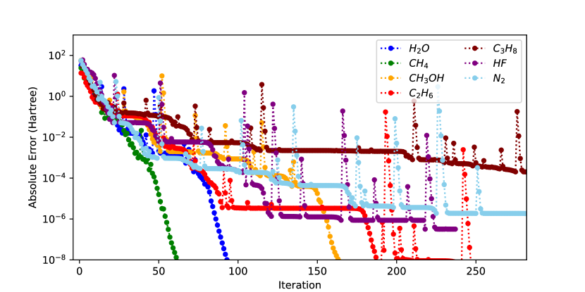
Figure 14: Convergence of the energy using $H^{\text{cheap}}_{\boldsymbol{x}}$ exactly and equation (30) to approximate $H^{\exp}$.

In subsection 4.2 we attributed the initial good convergence of the $B_{\boldsymbol{x}}=H^{\text{cheap}}_{\boldsymbol{x}}$ approximation to a sufficient approximation of the hessian. To take full advantage of the good convergence of $B_{\boldsymbol{x}}^{\exp}=0$, we then decided to turn on the ($\boldsymbol{x}$ and $\boldsymbol{\nu}$)BFGS approximation of $H^{\exp}$ only when the algorithm start to converge with $B_{\boldsymbol{x}}=H^{\text{cheap}}_{\boldsymbol{x}}$, to correct the convergence if it was not going to an actual minimum. Since $H^{\text{cheap}}_{\boldsymbol{x}}$ approximated the ON block of the hessian particularly well, it seems reasonable to look primarily at the ON step. In practice, we add a factor $A(s_{n},\epsilon)=\frac{1}{2}\bigl{[}1-\erf\bigl(\log_{10}(\absolutevalue{s_{n}}_{\infty}/\epsilon)\bigr{missing})\bigr{]}$ to $B_{\boldsymbol{x}}^{\exp}$, where $|s_{n}|_{\infty}$ is the $\infty$-norm of the ON step.
We report the result for $\boldsymbol{x}$BFGS in Fig. 15 and $\boldsymbol{\nu}$BFGS in Fig. 16. By comparing Fig. 14 and Fig. 16 we see that the prefactor $A$ significantly improves the convergence, even beyond the first few iterations. Although the convergence is not as good as for the exact hessian (Fig. 5) both approximations outperform the best BFGS approximation of the total hessian in the $\boldsymbol{\nu}$-space, see 12, reaching an error of $2\cdot 10^{-8}$ Hartree within 280 iterations for all molecules, and will reach $\cdot 10^{-8}$ with a few more iterations with a stronger termination condition. The $\boldsymbol{\nu}$BFGS approximation seems better for small molecules (H2O, CH4 and HF), suggesting that $\boldsymbol{\nu}$BFGS may retain more of the behaviour of $B_{\boldsymbol{x}}=H^{\text{cheap}}_{\boldsymbol{x}}$ but is not systematically better than $\boldsymbol{x}$BFGS (see convergence N2 and C2H6).

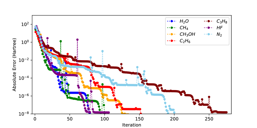
Figure 15: Convergence of the energy using $H^{\text{cheap}}_{\boldsymbol{x}}$ exactly and equation (28) to approximate $H_{\boldsymbol{x}}^{\exp}$ with the prefactor $A(s_{n},10^{-3})$ (see text).

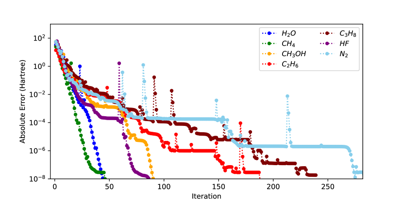
Figure 16: Convergence of the energy using $H^{\text{cheap}}_{\boldsymbol{x}}$ exactly and equation (30) to approximate $H_{\boldsymbol{x}}^{\exp}$ with the prefactor $A(s_{n},10^{-3})$ (see text).

It may be informative to look at the evolution of $A$ to understand the plateaus in the convergence of the energy for some molecules using $B^{\exp}_{\boldsymbol{\nu}}$. We plot $A$ and $|s_{n}|$ as functions of the iteration in Fig. 17. Only the result for the CH3OH molecule is reported here, but the results are qualitatively similar for the other molecules that do not converge with the $B^{\exp}=0$ approximation. We observe that $A$ does go from 0 to 1, but oscillates, inducing the plateaus in Fig. 16. This indicates that the choice of $A$ is not optimal and that the algorithm can be improved by building a better prefactor.

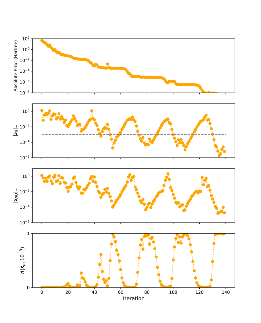
Figure 17: Absolute energy error, value of the $\infty$-norm of the ON step, NO step and the prefactor $A(s_{n},10^{-3})$ used on $B^{\exp}$ in $\boldsymbol{\nu}$-space w.r.t. the iteration during the SCF procedure, using equation (28),for the CH3OH molecule. The value $\epsilon=10^{-3}$ is shown (grey line) in the second panel.

6 Conclusion

In this work, we used an optimisation based on the hessian to reduce the number of iterations of the SCF-RDMFT procedure. We first added the cross terms in the hessian, providing an efficient 1-step optimisation method, in contrast to the more common 2-step one. As a baseline, we have shown that the a trust region optimization with the exact hessian provides a very effective algorithm for this. However, using the exact hessian, makes the iterations too expensive to be useful in practice. Thus we have investigated several cheap approximations to the hessian to come to a practical algorithm. We first extracted an affordable part of the exact hessian. Using only this cheap part, the number of iterations is actually of similar order as for the exact hessian if it converged, but half of our test set actually did not converge. The alternative to use the BFGS approximation directly for the hessian in parametrization space ($\boldsymbol{x}$-space) or the more suitable $\boldsymbol{\nu}$-space gave algorithms which roughly took more than an order of magnitude more iterations if they converged. A rather robust and effective approximation was obtained by combining the two approximations: use the cheap part of the hessian exactly and use a BFGS-like approximation to only approximate the expensive part (in $\boldsymbol{\nu}$-space). This approximate hessian resulted in an algorithm which converged for all seven molecules within a few hundred iterations.

Although the numerical results show a great amelioration of the convergence compared to a naive algorithm, we are still far away from the convergence we could expect when comparing to the case of the exact hessian. To enhance the convergence even further, a more accurate approximation of the hessian seems to be required. A first step in this direction would be to build a consistent secant equation in $\boldsymbol{x}$-space.

The plateaus in the energy versus iteration might indicate that the algorithm is struggling with relatively flat areas in the energy landscape. This might also explain why when using even the exact hessian, convergence is not that fast as one would expect. So another direction to improve the algorithm would thus be to help the algorithm getting away from these flat areas, by adapting ideas from global optimization for instance.

We have only used the Müller functional in our tests to avoid any additional non-convexity and discontinuity issues for the moment. These approximations to the expensive hessian part therefore still need to be tested with more advanced RDMFT functionals. The authors thank the The Netherlands Organisation for Scientific Research, NWO, for its support (Grant No. OCENW.KLEIN.434). Financial support from the NWO under Vici Grant No. 724.017.001 is acknowledged by KJHG.

Appendix A Expression of the exact hessian

The derivatives of the 1-RDM w.r.t. to the $x_{i}$ are obtained by simply taking the derivative of the NOs in (7). Likewise, we get the cross-derivative of the 1-RDM by taking the derivative of the NOs w.r.t. the $x_{i}$ in (9a).
Inserting the derivatives of the 1-RDM in (4.1) we get, for the NO block of the hessian

$$\left.\frac{\partial^{2}E_{1}}{\partial x_{i}\partial x_{j}}\right|_{0} =\sum_{p}\frac{\partial^{2}n_{p}}{\partial x_{i}\partial x_{j}}H^{1}_{pp}$$ (31)

$$\left.\frac{\partial^{2}E_{H}}{\partial x_{i}\partial x_{j}}\right|_{0} =\sum_{pq}\left(\frac{\partial^{2}n_{p}}{\partial x_{i}\partial x_{j}}n_{q}+\frac{\partial n_{p}}{\partial x_{i}}\frac{\partial n_{q}}{\partial x_{j}}\right)[pp|qq]$$ (32)

$$\left.\frac{\partial^{2}W_{\boldsymbol{xc}}}{\partial x_{i}\partial x_{j}}\right|_{0} =\sum_{pq}\frac{\partial^{2}F(n_{p},n_{q})}{\partial x_{i}\partial x_{j}}[pq|pq],$$ (33)

for the coupling block,

$$\left.\frac{\partial^{2}E_{1}}{\partial X_{ij}\partial x_{k}}\right|_{0} =2\left(\frac{\partial n_{i}}{\partial x_{k}}-\frac{\partial n_{j}}{\partial x_{k}}\right)H^{1}_{ij}$$ (34)

$$\left.\frac{\partial^{2}E_{H}}{\partial X_{ij}\partial x_{k}}\right|_{0} =2\sum_{p}\left((n_{i}-n_{j})\frac{\partial n_{p}}{\partial x_{k}}+(\frac{\partial n_{i}}{\partial x_{k}}-\frac{\partial n_{j}}{\partial x_{k}})n_{p}\right)[ij|pp]$$ (35)

$$\left.\frac{\partial^{2}W_{\boldsymbol{xc}}}{\partial X_{ij}\partial x_{k}}\right|_{0} =\sum_{p}\left(\frac{\partial F(n_{i},n_{p})}{\partial x_{k}}-\frac{\partial F(n_{j},n_{p})}{\partial x_{k}}\right)[ip|jp]+\left(\frac{\partial F(n_{p},n_{i})}{\partial x_{k}}-\frac{\partial F(n_{p},n_{j})}{\partial x_{k}}\right)[jp|ip]$$ (36)

$$=2\sum_{p}\left(\frac{\partial F(n_{i},n_{p})}{\partial x_{k}}-\frac{\partial F(n_{j},n_{p})}{\partial x_{k}}\right)[ip|jp],$$ (37)

if $F(n_{i},n_{j})=F(n_{j},n_{i})$, which holds for all functionals we are aware of. And, for the ON block, we get

$$\begin{split}\left.\frac{\partial^{2}E_{1}}{\partial X_{ij}\partial X_{pq}}\right|_{0}&=\delta_{ip}(2n_{i}-n_{j}-n_{q})H^{1}_{jq}+\delta_{jq}(2n_{j}-n_{i}-n_{p})H^{1}_{ip}\\ &-\delta_{iq}(2n_{i}-n_{j}-n_{p})H^{1}_{jp}-\delta_{jp}(2n_{j}-n_{i}-n_{q})H^{1}_{iq},\end{split}$$ (38)

$$\begin{split}\left.\frac{\partial^{2}E_{H}}{\partial X_{ij}\partial X_{pq}}\right|_{0}=\sum_{k}&\left(\hskip 8.0pt2\delta_{pi}(2n_{i}n_{k}-n_{j}n_{k}-n_{q}n_{k})[qj|kk]\right.+2\delta_{qj}(2n_{j}n_{k}-n_{i}n_{k}-n_{p}n_{k})[ip|kk]\\ &-2\delta_{iq}(2n_{i}n_{k}-n_{j}n_{k}-n_{p}n_{k})[jp|kk]-\left.2\delta_{jp}(2n_{j}n_{k}-n_{i}n_{k}-n_{q}n_{k})[iq|kk]\right)\\ &+4(n_{i}n_{p}-n_{j}n_{p}-n_{i}n_{q}+n_{j}n_{q})[ij|pq],\end{split}$$ (39)

$$\begin{split}\left.\frac{\partial^{2}W_{\boldsymbol{xc}}}{\partial X_{ij}\partial X_{pq}}\right|_{0}=\sum_{k}&\left(\hskip 8.0pt2\delta_{pi}(2F(n_{i},n_{k})-F(n_{j},n_{k})-F(n_{q},n_{k}))[qk|jk]\right.\\ &+2\delta_{qj}(2F(n_{j},n_{k})-F(n_{i},n_{k})-F(n_{p},n_{k}))[ik|pk]\\ &-2\delta_{iq}(2F(n_{i},n_{k})-F(n_{j},n_{k})-F(n_{p},n_{k}))[jk|pk]\\ &-\left.2\delta_{jp}(2F(n_{j},n_{k})-F(n_{i},n_{k})-F(n_{q},n_{k}))[ik|qk]\right)\\ &+4(F(n_{i},n_{p})-F(n_{j},n_{p})-F(n_{i},n_{q})+F(n_{j},n_{q}))[ip|jq].\end{split}$$ (40)

Appendix B Derivation of the BFGS approximation

The idea of (quasi-)Newton methods is to take the derivative of a second order model $m$ of the function $f$ to optimise, which writes for the $k^{th}$ iteration

$$\gradient m^{(k)}(p)=\gradient f^{(k)}+B^{(k)}p,$$ (41)

where $B$ is the (approximate) hessian. We then impose that the derivative of $m$ coincides with the derivative of $f$ at the last two iterations. For the last iterations it is automatically verified by taking $p=0$, and for the second last iterations we have to take $p=-s^{(k-1)}$, that is, the opposite of the last step, and we get

$$\gradient m^{(k)}(-s^{(k-1)})=\gradient f^{(k)}-B^{(k)}s^{(k-1)}=\gradient f^{(k-1)}.$$ (42)

By defining $y^{(k-1)}=\gradient f^{(k)}-\gradient f^{(k-1)}$, we obtain the, so called, secant equation,

$$B^{(k+1)}s^{(k)}=y^{(k)}.$$ (43)

To obtain the BFGS update (16), we need to solve problem (15)

$$\min_{B\in\mathds{R}^{N\times N}}\norm{B-B^{(k)}}\quad\text{ s.t. }\quad B^{T}=B\text{ and }Bs^{(k)}=y^{(k)},$$ (44)

with the Frobenius norm for $\norm{\cdot}$.

We follow the proof given by Hauser ⁵⁰. To ensure that $B$ is symmetric, we write it as $B=LL^{T}$, $L\in\mathds{R}^{N\times N}$. Taking $g=L^{T}s^{(k)}$ the secant equation becomes

$$Lg=y^{(k)}.$$ (45)

Taking the scalar product $\innerproduct{A}{B}=\Tr(AB^{T})$, (44) is equivalent to

$$\min_{L}\innerproduct{L-L^{(k)}}{L-L^{(k)}}\quad\text{s.t.}\quad\innerproduct{L}{e_{i}g^{T}}=y^{(k)}_{i}\forall i,$$ (46)

with $e_{i}$ the $i^{th}$ column of the identity matrix, that is $e_{i}g^{T}$ are the normal vectors defining the affine subspace $\mathcal{P}_{g}$ in which $L$ has to be optimised. The minimizer $L^{*}$ is the closest point to $L^{(k)}$ in $\mathcal{P}_{g}$. Thus, $L^{*}-L^{(k)}$ is orthogonal to $\mathcal{P}_{g}$ and so a linear combination of the $e_{i}g^{T}$. Equation (44) is then equivalent to find $L^{*}\in\mathds{R}^{N\times N}$ and $\lambda^{*}\in\mathds{R}^{N}$ satisfying

$$(L^{*}-L^{(k)})-\lambda^{*}g^{T} =0$$ (47a)

$$L^{*}g =y^{(k)}.$$ (47b)

Multiplying (47a) from the right by $g$ and utilizing (47b) gives

$$\lambda^{*} =\frac{y^{(k)}-L^{(k)}g}{g^{T}g},$$ (48a)

which can be inserted back to yield

$$L^{*} =L^{(k)}+\frac{(y^{(k)}-L^{(k)}g)g^{T}}{g^{T}g}.$$ (48b)

Inserting the minimizer $L^{*}$ in the definition of $g$ and rearranging gives

$$L^{(k)T}s^{(k)}=g\left(1-\frac{(y^{(k)}-L^{(k)}g)^{T}s^{(k)}}{g^{T}g}\right),$$ (49)

meaning that $g\propto L^{(k)T}s^{(k)}$. We take $g=\beta L^{(k)T}s^{(k)}$ and by inserting it into the previous equation, we get $\beta=\pm\sqrt{\frac{y^{(k)T}s^{(k)}}{s^{(k)T}B^{(k)}s^{(k)}}}$. We now have an explicit expression for $L^{*}$ and simplifying $B^{(k+1)}\equiv B^{*}\equiv L^{*}L^{*T}$ we get the BFGS approximation (16).

References

- Geerlings et al. 2003 Geerlings, P.; De Proft, F.; Langenaeker, W. Conceptual Density Functional Theory. Chemical Reviews 2003, 103, 1793–1874, PMID: 12744694
- Dreizler and Gross 2012 Dreizler, R. M.; Gross, E. K. U. Density Functional Theory; Springer Berlin, Heidelberg, 2012
- Kohn et al. 1996 Kohn, W.; Becke, A. D.; Parr, R. G. Density Functional Theory of Electronic Structure. The Journal of Physical Chemistry 1996, 100, 12974–12980
- Baerends and Gritsenko 1997 Baerends, E. J.; Gritsenko, O. V. A Quantum Chemical View of Density Functional Theory. The Journal of Physical Chemistry A 1997, 101, 5383–5403
- Mardirossian and Head-Gordon 2017 Mardirossian, N.; Head-Gordon, M. Thirty years of density functional theory in computational chemistry: an overview and extensive assessment of 200 density functionals. Molecular Physics 2017, 115, 2315–2372
- Orio et al. 2009 Orio, M.; Pantazis, D.; Neese, F. Density functional theory. 2009,
- Bartolotti and Flurchick 1996 Bartolotti, L. J.; Flurchick, K. An introduction to density functional theory; Wiley Online Library, 1996; Chapter 4. An Introduction to Density Functional Theory, pp 187–216
- Cohen et al. 2012 Cohen, A. J.; Mori-Sánchez, P.; Yang, W. Challenges for Density Functional Theory. Chemical Reviews 2012, 112, 289–320, PMID: 22191548
- Bally and Sastry 1997 Bally, T.; Sastry, G. N. Incorrect Dissociation Behavior of Radical Ions in Density Functional Calculations. Journal of Physical Chemistry A 1997, 101, 7923–7925
- Braïda et al. 1998 Braïda, B.; Hiberty, P. C.; Savin, A. A Systematic Failing of Current Density Functionals: Overestimation of Two-Center Three-Electron Bonding Energies. The Journal of Physical Chemistry A 1998, 102, 7872–7877
- Ossowski et al. 2003 Ossowski, M. M.; Boyer, L. L.; Mehl, M. J.; Pederson, M. R. Water molecule by the self-consistent atomic deformation method. Phys. Rev. B 2003, 68, 245107
- Grüning et al. 2003 Grüning, M.; Gritsenko, O. V.; Baerends, E. J. Exchange-correlation energy and potential as approximate functionals of occupied and virtual Kohn–Sham orbitals: Application to dissociating H2. The Journal of Chemical Physics 2003, 118, 7183–7192
- Ruzsinszky et al. 2006 Ruzsinszky, A.; Perdew, J. P.; Csonka, G. I.; Vydrov, O. A.; Scuseria, G. E. Spurious fractional charge on dissociated atoms: Pervasive and resilient self-interaction error of common density functionals. The Journal of Chemical Physics 2006, 125, 194112
- Wagner et al. 2014 Wagner, L. O.; Baker, T. E.; Stoudenmire, E. M.; Burke, K.; White, S. R. Kohn-Sham calculations with the exact functional. Phys. Rev. B 2014, 90, 045109
- Piris and Ugalde 2009 Piris, M.; Ugalde, J. M. Iterative diagonalization for orbital optimization in natural orbital functional theory. Journal of Computational Chemistry 2009, 30, 2078–2086
- Pernal and Giesbertz 2016 Pernal, K.; Giesbertz, K. J. Reduced density matrix functional theory (RDMFT) and linear response time-dependent RDMFT (TD-RDMFT). Density-Functional Methods for Excited States 2016, 125–183
- Lemke et al. 2022 Lemke, Y.; Kussmann, J.; Ochsenfeld, C. Efficient integral-direct methods for self-consistent reduced density matrix functional theory calculations on central and graphics processing units. Journal of Chemical Theory and Computation 2022, 18, 4229–4244
- Gilbert 1975 Gilbert, T. L. Hohenberg-Kohn theorem for nonlocal external potentials. Phys. Rev. B 1975, 12, 2111–2120
- Levy 1979 Levy, M. Universal variational functionals of electron densities, first order density matrices, and natural-spinorbitals and solutions of the -representability problem. Proc. Natl. Acad. Sci. USA 1979, 76, 6062–6065
- Valone 1980 Valone, S. M. Consequences of extending 1-matrix energy functionals from pure–state representable to all ensemble representable 1 matrices. J. Chem. Phys. 1980, 73, 1344–1349
- Goedecker and Umrigar 1998 Goedecker, S.; Umrigar, C. J. Natural Orbital Functional for the Many-Electron Problem. Phys. Rev. Lett. 1998, 81, 866–869
- Gritsenko et al. 2005 Gritsenko, O.; Pernal, K.; Baerends, E. J. An improved density matrix functional by physically motivated repulsive corrections. The Journal of chemical physics 2005, 122
- Piris et al. 2010 Piris, M.; Matxain, J.; Lopez, X.; Ugalde, J. Communications: Accurate description of atoms and molecules by natural orbital functional theory. The Journal of chemical physics 2010, 132
- Piris et al. 2011 Piris, M.; Lopez, X.; Ruipérez, F.; Matxain, J.; Ugalde, J. A natural orbital functional for multiconfigurational states. The Journal of chemical physics 2011, 134
- Piris 2017 Piris, M. Global method for electron correlation. Physical review letters 2017, 119, 063002
- Piris 2021 Piris, M. Global Natural Orbital Functional: Towards the Complete Description of the Electron Correlation. Phys. Rev. Lett. 2021, 127, 233001
- Cohen and Baerends 2002 Cohen, A. J.; Baerends, E. J. Variational density matrix functional calculations for the corrected Hartree and corrected Hartree–Fock functionals. Chem. Phys. Lett. 2002, 364, 409–419
- Pernal 2005 Pernal, K. Effective potential for natural spin orbitals. Physical review letters 2005, 94, 233002
- Baldsiefen and Gross 2013 Baldsiefen, T.; Gross, E. K. U. Minimization procedure in reduced density matrix functional theory by means of an effective noninteracting system. Comput. Theor. Chem. 2013, 1003, 114–122
- Löwdin 1955 Löwdin, P.-O. Quantum Theory of Many-Particle Systems. I. Physical Interpretations by Means of Density Matrices, Natural Spin-Orbitals, and Convergence Problems in the Method of Configurational Interaction. Phys. Rev. 1955, 97, 1474–1489
- Coleman 1963 Coleman, A. J. Structure of Fermion Density Matrices. Rev. Mod. Phys. 1963, 35, 668–687
- Herbert and Harriman 2003 Herbert, J. M.; Harriman, J. E. -representability and variational stability in natural orbital functional theory. J. Chem. Phys. 2003, 118, 10835
- Lathiotakis et al. 2007 Lathiotakis, N. N.; Helbig, N.; Gross, E. K. U. Performance of one-body reduced density-matrix functionals for the homogeneous electron gas. Phys. Rev. B 2007, 75, 195120
- Yao et al. 2021 Yao, Y.-F.; Fang, W.-H.; Su, N. Q. Handling Ensemble N-Representability Constraint in Explicit-by-Implicit Manner. The Journal of Physical Chemistry Letters 2021, 12, 6788–6793, PMID: 34270236
- Lathiotakis and Marques 2008 Lathiotakis, N. N.; Marques, M. A. L. Benchmark Calculations for reduced density-matrix functional theory. J. Chem. Phys. 2008, 128, 184103
- Douady et al. 1980 Douady, J.; Ellinger, Y.; Subra, R.; Levy, B. Exponential transformation of molecular orbitals: A quadratically convergent SCF procedure. I. General formulation and application to closed-shell ground states. The Journal of Chemical Physics 1980, 72, 1452–1462
- Cioslowski and Pernal 2001 Cioslowski, J.; Pernal, K. Response properties and stability conditions in density matrix functional theory. The Journal of Chemical Physics 2001, 115, 5784–5790
- Goedecker and Umrigar 2000 Goedecker, S.; Umrigar, C. J. In Many-Electron Densities and Reduced Density Matrices; Cioslowski, J., Ed.; Kluwer Academic: Dordrecht, 2000; Chapter 8, pp 165–181
- Piris 2006 Piris, M. A new approach for the two-electron cumulant in natural orbital functional theory. Int. J. Quantum Chem. 2006, 106, 1093–1104
- Müller 1984 Müller, A. Explicit approximate relation between reduced two-and one-particle density matrices. Physics Letters A 1984, 105, 446–452
- Buijse 1991 Buijse, M. A. PhD thesis. Ph.D. thesis, Vrije Universiteit, Amsterdam, 1991
- Frank et al. 2007 Frank, R. L.; Lieb, E. H.; Seiringer, R.; Siedentop, H. Müller’s exchange-correlation energy in density-matrix-functional theory. Phys. Rev. A 2007, 76, 052517
- Froehlich and Weindl 2021 Froehlich, F.; Weindl, D. Fides. 2021; https://github.com/dweindl/fides-cpp
- Coleman and Li 1994 Coleman, T. F.; Li, Y. On the convergence of interior-reflective Newton methods for nonlinear minimization subject to bounds. Mathematical Programming 1994, 67, 189–224
- Coleman and Li 1996 Coleman, T. F.; Li, Y. An Interior Trust Region Approach for Nonlinear Minimization Subject to Bounds. SIAM Journal on Optimization 1996, 6, 418–445
- Cancès and Pernal 2008 Cancès, E.; Pernal, K. Projected gradient algorithms for Hartree-Fock and density matrix functional theory calculations. The Journal of Chemical Physics 2008, 128, 134108
- Cayley 1846 Cayley, A. About the algebraic structure of the orthogonal group and the other classical groups in a field of characteristic zero or a prime characteristic. Reine Angewandte Mathematik 1846, 32, 6
- Giesbertz 2016 Giesbertz, K. J. H. Avoiding the 4-index transformation in one-body reduced density matrix functional calculations for separable functionals. Phys. Chem. Chem. Phys. 2016, 18, 21024–21031
- Nocedal and Wright 2006 Nocedal, J.; Wright, S. J. Numerical optimization, 2nd ed.; Springer New York, NY, 2006
- Hauser 2005 Hauser, R. Section: Continuous Optimisation Lectrue 4: Quasi-Newton Methods. University of Oxford, Honour School of Mathematics, 2005