Prepare Non-classical Collective Spin State by Reinforcement Learning

Abstract

We propose a scheme leveraging reinforcement learning to engineer control fields for generating non-classical states. It is exemplified by the application to prepare spin squeezed state for an open collective spin model where a linear control term is designed to govern the dynamics. The reinforcement learning agent determines the temporal sequence of control pulses, commencing from coherent spin state in an environment characterized by dissipation and dephasing. When compared to constant control scenarios, this approach provides various control sequences maintaining collective spin squeezing and entanglement. It is observed that denser application of the control pulses enhances the performance of the outcomes. Furthermore, there is a minor enhancement in the performance by adding control actions. The proposed strategy demonstrates increased effectiveness for larger systems. And thermal excitations of the reservoir are detrimental to the control outcomes. It should be confirmed that this is an open-loop strategy by closed-loop simulation, circumventing collapse of quantum state induced by measurements. Thanks to the flexible replaceability of the optimization modules and the controlled system, this research paves the way for its application in manipulating other quantum systems.

I introduction

Precise measurement for physical quantities has propelled advances in physics. The application of non-classical quantum states can open pathways toward precise measurement. Spin squeezed states are such a kind of pertinent candidates characterized by reduced uncertainty in a collective spin component. Entanglement typically arises concomitantly with spin squeezing, as a result of the interatomic interactions within an ensemble 8PR50989 ; 1RMP90035005 . Decreasing the variance of an observable leads to an escalation in measurement sensitivity that transcends the standard quantum limit within the realm of quantum-enhanced metrology. Such squeezed states can be used to enhance the performance of homodyne interferometers 2PRA46R6797 ; 3PRA5067 , magnetometers 4PRL109253605 , and atomic clocks 5RMP87637 . The evidence delineating the association between the sensitivity of phase estimation and entanglement was demonstrated in collective spin model 6PRL102100401 .

Many schemes have been proposed to prepare spin squeezed states based on the nonlinear squeezing term in the Hamiltonian 9PRA475138 ; 8PR50989 . For example, quantum non-demolition measurement can be used to generate spin squeezed states 10EL42481 . Some proposals are based on nonlinear interactions among the individual elements in Bose-Einstein condensates 12PRL853991 . Theoretically, coherent control has been proposed to produce spin squeezed states 13PRA63055601 . Long-lasting and extreme spin squeezed states is pursued all the way.

Machine-learning techniques are emerging as an effective tool in physics 14Murphy2012 , and among them, reinforcement learning (RL) offers the potential to optimize control for high-dimensional, multistage processes in complex scenarios. Deep reinforcement learning (DRL) can provide control strategy to engineer the dynamics as long as the evolution follows certain differential equations. In physics, many optimal problems can be treated as control problems of finding means to steer the systems to achieve a certain target. The search for optimal control field can be formulated as RL task 16Sutton2018 ; 17PRX8031084 ; 19MURPHY2012 . The estimation of the precession frequency of a dissipative particle was enhanced by adding a linear control in the form of an additional controlled magnetic field 20npj582 .

We propose a reinforcement-learning based control scheme to design control fields to prepare non-classical spin states. The agent is trained to produce a sequence of square pulses that steers the system evolving to squeezed states under the domain of Lindblad master equation. The generalization performance of the proposed control scheme was evaluated across a range of control parameters, system sizes, and thermal excitations.

This paper is organized as follows: In Sec.II, we delineate the reinforcement-learning-based framework for the preparation of nonclassical states. In Sec.III, the RL module employed within the control scheme is shown. In Sec.IV, we explicate the quantum model for the generation of spin-squeezed states. In Sec.V, we present the procedure to prepare squeezed states in the open collective spin system via reinforcement learning. In Sec.VI, we check the performance of this method including the influence of the frequency of applying the control pulses, the granularity of control actions, system scalability across various sizes, and the impact of thermal excitation. Finally, we conclude in Sec.VIII with a synopsis of the findings and potential avenues for future research.

II Control Scheme

Taking a cue from Lyapunov control strategies 24B.B42nd ; 25Auto411987 ; 26AC50768 ; 27JPB44195503 ; 54PLA378699 , we harness machine learning to design control fields that facilitate the preparation of nonclassical states. In the presence of a control field, the general total Hamiltonian for the quantum system reads: $\hat{H}=\hat{H}_{0}+\sum_{m=1}^{M}f_{m}(t)\hat{H}_{m}$, where $\hat{H}_{0}$ is the free Hamiltonian and $m$ denotes the number of external control Hamiltonians $\hat{H}_{m}$. $f_{m}(t)$ is the corresponding control field designed by RL in this work. It should be confirmed that $[\hat{H}_{0},\hat{H}_{m}]\neq 0$, otherwise, the influence of the control Hamiltonians can be subsumed into the free Hamiltonian.

This scheme is an open-loop application strategy, wherein the control fields are devised through the emulation of a closed-loop process, as shown in Fig. 1. Under the control designed by machine learning agent, the system would be steered to a set of states meeting the control target. Notably, the RL agents can be supplanted by alternative optimization modules tailored for the target. The proposed control scheme is applicable to other dynamical systems governed by certain differential equations. To illustrate the efficacy of the scheme, we have applied it to engineer a collective spin system.

III Machine Learning Tools: Reinforcement Learning

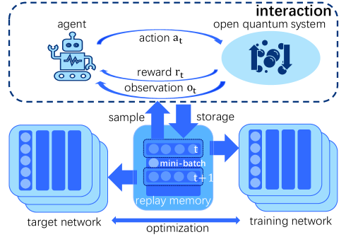
Figure 1: In RL, Q function is defined as $Q^{\pi}(s_{t},a_{t})=r(s_{t})+E_{\{(s_{t+i},a_{t+i})|\pi\}_{i=1}^{\infty}}\!\left[\sum_{i=1}^{\infty}\gamma^{i}_{q}\,r(s_{t+i})\right]$ where $\gamma_{q}$ ($0\!<\!\gamma_{q}\!<\!1$, usually close to 1) is a discount factor, and the expectation $E$ is taken over trajectories of the action and the state of the controlled system 29Nature518529 ; 30PNAS38716 . The optimal policy $\pi^{*}$ maximizing $Q$ value satisfies the Bellman equation $Q^{\pi^{*}}(s_{t},a_{t})=r(s_{t})+\gamma_{q}\,E_{s_{t+1}}\left[\max_{a_{t+1}}Q^{\pi^{*}}(s_{t+1},a_{t+1})\right].$ Once the equation of $Q^{\pi^{*}}$ were satisfied, the optimal policy $\pi^{*}$ is determined. The schematic of the training procedure involves: 1. The agent provides actions $a_{t}$ to steer the open quantum system (the ‘environment’ in RL), and receives observations $\sigma_{t}$ and rewards $r_{t}$. 2. These experiences are stored in the replay memory as state-action-reward combination of map. 3. The agent randomly samples batches of the combinations from the replay memory to train the neural network to minimize the difference between the predicted Q-values and the target Q-values. 4. The target Q-values are computed by considering the immediate reward and the estimated maximum future rewards, which contributes to stabilize the training process based on the next state, using the Q-network weights from the previous iteration. 5. The process including interaction, experience replay, and network updates is repeated to iteratively improve the Q-function approximation.

Initiating with no priori knowledge about the dynamics of the system under control, RL adopts a trial-and-error manner to iteratively learn a mapping that determines an action depending on different states under certain rules, namely, aimed at maximizing the accumulated reward over discrete time instances $t$. Rewards are obtained using an evaluation rule that aligns with the control objectives. An appropriate rewards-evaluation rule that favors particular state-action mappings can enhance the control performance. Decision-making executed by the agent entails selecting actions $a_{t}=\pi(s_{t})$ that affect the system changing from a state (not specifically referring to quantum states, but a general state characterized by various quantities of a controlled system) $s_{t}$ to $s_{t+1}$, with $\pi$ denoting the policy being refined.

Q-learning realizes RL through a Q function that represents the expected total future reward of a policy $\pi$. The optimal policy $\pi^{*}$ with maximized $Q$ function satisfies Bellman equation 29Nature518529 ; 30PNAS38716 . Deep Q-learning uses a deep feed-forward neural network to approximate this function 31Nature521436 ; 32GoodfellowDL ; 33arXiv171002298 , and the network is called a deep Q network (DQN) denoted by $W_{\theta}(s,a)$, where $\theta$ represents the net parameters need to be adjusted by training, and the controlled system state $s$ is the network input. Assuming that the space of actions $a$ is discrete, the DQN outputs a value for each choice of action $a$. DQN leverages extensive datasets that encapsulate the anticipated cumulative rewards consequent to specific actions within distinct states, facilitating the neural network-based approximation of the conventional action-value function 62TR2001 ; 61CS2500611 ; 64PMLR387395 ; 66PMLR19281937 ; 65arXiv150902971 ; 37arXiv151106581 .

In this study, the DQN algorithm is incorporated into the reinforcement learning framework to determine an optimized control strategy. It should be noted that, depending on particular needs and constraints of tasks, alternative optimization algorithms could be employed in place of the DQN.

IV Collective Spin Model

We consider an ensemble of $N$ identical two-level atoms with pseudo spin components $\hat{J}_{\alpha}=\frac{1}{2}\sum^{N}_{k=1}\hat{\sigma}_{\alpha}^{(k)}$, $(\alpha=x,y,z)$, where $\hat{\sigma}_{\alpha}^{(k)}$ is the Pauli operator for the $k$-th atom 38PRA62211 . This is the symmetric scenario where the operations done on the ensemble have identical impact on all the atoms. $\hat{J}_{x}$, $\hat{J}_{y}$, $\hat{J}_{z}$ fulfill the SU(2) commute relationship: $[\hat{J}_{\alpha},\hat{J}_{\beta}]=i\hbar\epsilon_{\alpha\beta\gamma}\hat{J}_{\gamma}$, where $\epsilon_{\alpha\beta\gamma}$ is the Lévi-Cività symbol. The total collective spin length is specified by $J=N/2$ while the dimension of the Hilbert space is $2J+1=N+1$. The collective spin can be mapped to its two-mode bosonic partner by Schwinger transformation: $\hat{J}_{z}=\frac{1}{2}(\hat{a}^{\dagger}\hat{a}-\hat{b}^{\dagger}\hat{b})$, $\hat{J}_{+}=\hat{a}^{\dagger}\hat{b}$ and $\hat{J}_{-}=(\hat{J}_{+})^{\dagger}$, where $\hat{a}$ and $\hat{b}$ are the two annihilation operators of two boson modes 67AMQP . In this view, by mapping one mode to spin up and the other one to spin down, $\hat{J}_{z}$ reflects the population difference between the two modes in Ramsey interferometer 2PRA46R6797 ; 9PRA475138 ; 1RMP90035005 .

To examine the effectiveness of the proposal, we focus on a collective spin system described by the Hamiltonian

$$\hat{H}/\hbar=\kappa\hat{J}_{z}^{2}+\Omega_{x}(t)\hat{J}_{x},$$ (1)

here $\kappa$ indicates the strength of the interaction between the atoms and the time scales as $\kappa t$. $\kappa$ would be taken as the unit ($\kappa$=1 herafter) and the natural units ($\hbar=1$) is used. $\hat{J}_{z}^{2}$ refers to the one-axis twisting which induces spin squeezing 9PRA475138 . This squeezing provides the resource for quantum-enhanced metrology 9PRA475138 ; 1RMP90035005 . $\hat{J}_{x}$ is the control Hamiltonian describing the magnetic field in $x$-direction, or the counterpart, the linear beam splitters in interferometers).

In contrast to the application of a constant control 13PRA63055601 , the present proposal employs RL agent designing time-dependent control fields $\Omega_{x}(t)$ to prepare nonclassical states. The temporally varying control field can represent the operational analogy of linear beam splitters in interferometric experiments. Since $[\hat{J}_{z}^{2},\hat{J}_{x}]=i\hbar(\hat{J}_{y}\hat{J_{z}}+\hat{J}_{z}\hat{J}_{y})$, such a linear control Hamiltonian can be used to steer the ensemble.

Spin squeezing can be quantified by using parameters constructed by the expected values of collective spin operators 8PR50989 ; 1RMP90035005 . Upon the reduction of the variances beneath the standard quantum limit threshold, the system is rendered applicable for precision metrology, along with amplifying the variance of the orthogonal spin components. We should confirm that the minimum squeezing parameter reads

$$\xi_{\perp}^{2}=\frac{N\min(\Delta\hat{J}_{\vec{n}_{\perp}}^{2})}{|\langle\hat{J}_{s}\rangle|^{2}}=\frac{N\left[\left\langle\hat{J}_{\vec{n}_{1}}^{2}+\hat{J}_{\vec{n}_{2}}^{2}\right\rangle-\sqrt{\left\langle\hat{J}_{\vec{n}_{1}}^{2}-\hat{J}_{\vec{n}_{2}}^{2}\right\rangle^{2}+\langle\left[\hat{J}_{\vec{n}_{1}},\hat{J}_{\vec{n}_{2}}\right]_{+}\rangle^{2}}\right]}{2|\langle\hat{J}_{s}\rangle|^{2}},$$ (2)

where $\hat{J}_{\vec{n}_{i}}$=$(\hat{J}_{x},\hat{J}_{y},\hat{J}_{z})\cdot\vec{n}_{i}$, ($i=1,2$) and $\vec{n}_{1}=(-\sin{\phi},\cos{\phi},0)$, $\vec{n}_{2}=(\cos{\theta}\cos{\phi},\cos{\theta}\sin{\phi},-\sin{\theta})$, $\hat{J}_{s}$=$(\hat{J}_{x},\hat{J}_{y},\hat{J}_{z})\cdot(\sin\theta\cos\phi,\sin\theta\sin\phi,\cos\theta)$, where $\theta$ = $\arccos(\frac{\langle J_{z}\rangle}{|{\hat{J}}|})$, $\phi$ = $\mathrm{sign}(\langle\hat{J}_{y}\rangle)\arccos(\frac{\langle\hat{J}_{x}\rangle}{|{\hat{J}}|\sin\theta})$, $|{\hat{J}}|=\sqrt{\langle\hat{J}_{x}\rangle^{2}+\langle\hat{J}_{y}\rangle^{2}+\langle\hat{J}_{z}\rangle^{2}}$ 8PR50989 ; 1RMP90035005 ; JPB39559 . The direction $\vec{n}_{\perp}$=$\vec{n}_{1}\cos\varphi+\vec{n}_{2}\sin\varphi$ with

$$\varphi=\left\{\begin{array}[]{ll}\frac{1}{2}\arccos\Big{(}\frac{-A}{\sqrt{A^{2}+B^{2}}}\Big{)}&\text{if}~{}~{}B\leq 0,\\ \pi-\frac{1}{2}\arccos\Big{(}\frac{-A}{\sqrt{A^{2}+B^{2}}}\Big{)}&\text{if}~{}~{}B>0,\end{array}\right.$$ (3)

where

$$A\equiv\langle J_{\vec{n}_{1}}^{2}-J_{\vec{n}_{2}}^{2}\rangle,\text{ \ }\;B\equiv\langle\left[\hat{J}_{\vec{n}_{1}},\hat{J}_{\vec{n}_{2}}\right]_{+}\rangle.$$ (4)

In this control scheme, we employ the following defination

$$\xi_{Z}^{2}=\frac{N\Delta\hat{J}_{z}^{2}}{|\langle\hat{J}_{s}\rangle|^{2}},$$ (5)

as the squeezing parameter. Here $\Delta\hat{J}_{z}^{2}$= $\langle\hat{J}_{z}^{2}\rangle-\langle\hat{J}_{z}\rangle^{2}$, indicates the spin squeezing in z-direction. For RL, we use the reverse of $\xi_{Z}^{2}$ to set the reward-punishment rule during the control process. Subsequently, in accordance with the fundamental principles of RL, the agent will steer the direction with minimum squeezing parameter approaching $z$ direction, namely, $\varphi=\pi/2$ in Eq. 3. And compared to using the reverse of $\xi_{R}^{2}$ with variable $\theta$ and $\phi$, the choice of $\xi_{Z}^{2}$ possesses a more direct physical interpretation since $\hat{J}_{z}$ signifies the population imbalance between the two modes within the Ramsey interferometer mentioned above 2PRA46R6797 ; 9PRA475138 ; 1RMP90035005 .

Correlation exists between entanglement and spin squeezing 42PRL864431 , wherein multipartite entanglement constitutes a quantum resource for enhanced precision in metrology 6PRL102100401 ; 43PRA85022322 ; 44Science3061330 . Moreover, Quantum Fisher information (QFI) quantifies the link between entanglement and phase uncertainty within the domain of metrology  45JSP1231 ; 46Science345424 . Adhering to the quantum Cramer-Rao bound, quantum states with larger QFI are pursued for the efficacy of quantum metrology 47PLA25101 ; 48PRL723439 . We would check the QFI pertaining to collective spin state $\hat{\rho}$ with respect to $\hat{\rho}(\theta)=e^{i\theta\hat{G}}\hat{\rho}e^{-i\theta\hat{G}}$, where $\theta$ is the quantity which needs to be estimated with respect to the phase-shift operator $\hat{G}$ 50PRA88043832 ; SR58565 . The QFI reads

$$F(\rho,\hat{G})=4\sum_{n}p_{n}(\Delta\hat{G})_{n}^{2}-\sum_{m\neq n}\frac{8p_{m}p_{n}}{p_{m}+p_{n}}|\langle\psi_{m}|\hat{G}|\psi_{n}\rangle|^{2},$$ (6)

where $\rho|\psi_{n}\rangle$=$p_{n}|\psi_{n}\rangle$, and $(\Delta\hat{G})_{n}^{2}\equiv\langle\psi_{n}|\hat{G}^{2}|\psi_{n}\rangle-|\langle\psi_{n}|\hat{G}|\psi_{n}\rangle|^{2}$. The second term denotes a correction. Here, the quantum Fisher information provides a quantitative threshold for the precision attainable in estimating $\theta$ by measuring $\hat{G}$ on $\rho$. If the average quantum Fisher information over three basic directions reaches the order of 1, there is macroscopic multiparticle entanglement 51PRA85022321 .

V Prepare spin squeezed state by reinforcement learning

There are mainly two steps to prepare the spin squeezed states: firstly, spin coherent state should be prepared, and secondly, spin squeezed state is prepared by using the control field designed by machine learning agent.

V.1 Initial Spin Coherent State

$N$ two-level atoms all pointing along the same direction can be described by an SU(2) spin coherent state (CSS). Such a state reads

$$|\theta,\phi\rangle=(\cos\frac{\theta}{2})^{2j}\sum_{m=-j}^{j}(C_{j+m}^{2j})^{1/2}[e^{-i\phi}\tan\frac{\theta}{2}]^{j+m}|j,m\rangle,$$ (7)

where $C_{j+m}^{2j}$ are the binomial coefficients. This state is most similar to classical state of a collective spin with $\theta$ and $\phi$ being the azimuth angles for longitude and latitude, respectively. $|j,m\rangle$ are the eigenvectors satisfy the equations $\hat{J}^{2}|j,m\rangle$=$j(j+1)\hbar^{2}|j,m\rangle$ and $\hat{J}_{z}|j,m\rangle$=$m\hbar|j,m\rangle$ ($\hbar$=1 in numerical calculations). The quantum state can be represented by the Husimi function or the Wigner distribution.

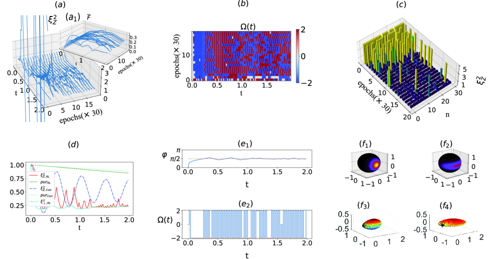
Figure 2: $(a)$ Evolution of the spin squeezing parameter (5) versus training epochs while 100 segments of actions are evenly taken across each evolution time interval $[0,2]$. We show a sample every 30 training epochs within 600 consecutive training rounds. The subfigure in $(a_{1})$ shows the evolution of the corresponding averaged quantum Fisher information defined as $\bar{F}$=$[F(\rho,\hat{J}_{x})+F(\rho,\hat{J}_{y})+F(\rho,\hat{J}_{z})]/(3N^{2})$. $(b)$ The top view of the 3-action ($\Omega(t)=2,0,-2$) square control pulse corresponding to the spin squeezing curves in $(a)$. $(c)$ 30 samples (differentiate by $n$) of the squeezing parameter at $t=2$ of those each 30 epochs in $(a)$. As shown in Figure $(a)$, there are control sequences causing $\xi_{Z}^{2}$ to diverge. However, such control sequences will not be accepted. Therefore, we express instances where $\xi_{Z}^{2}>5$ uniformly as 5 to facilitate the visualization of the results in $(c)$. $(d)$ The squeezing parameters versus time for the constant coherent control ($\Omega(t)=-2$) and the RL-designed control, with the corresponding degree of mixing ($Tr[\rho^{2}(t)]$). The subscript $RL$ means $\Omega(t)$ obtained by reinforcement learning, $Con$ means $\Omega(t)=-2$. $(e_{1})$ evolution of the angle $\varphi$ in Eq. 3. $(e_{2})$ The control fields $\Omega(t)$ designed by RL agent corresponding to $(d)$ and the constant control field $\Omega(t)=-2$. $(f_{1})$ and $(f_{2})$ are the Husimi representation of the initial CSS and the squeezed state at $t=2$. $(f_{3})$ and $(f_{4})$ are the polar plots of the Wigner function for the states. We use $N$=$2J$=20. The decaying parameters are $\gamma$=0.001$\kappa$.

The CSS can be prepared by applying a $\pi/2$ pulse to a BEC with $N$ atoms in the internal ground state 52nature40963 . In the CSS, $\langle\hat{J}_{x}\rangle=N/2$ and $\langle\hat{J}_{y}\rangle=\langle\hat{J}_{z}\rangle=0$. Such a pulse is equivalent to the effect of a beam splitter in interferometer.

Commencing with a CSS aligned along the $x$-axis and characterized by isotropic fluctuation in its spin components, $\hat{J}_{z}^{2}$ shears the coherent state to a squeezed one with reduced variance of $\hat{J}_{z}$, culminating in the generation of a squeezed spin state. Such states exceed the constraints delineated by the standard quantum limit, allowing for the enhanced measurement sensitivity in metrology along the squeezed direction 6PRL102100401 . The squeezed direction would be fixed on $\hat{J}_{z}$ under the action of $\Omega(t)\hat{J}_{x}$ determined by the reinforcement learning agent as mentioned above.

V.2 Prepare spin squeezed states by machine designed pulses

Usually, it is hard to avoid decoherence in a quantum system due to its interaction with the environment. The control scheme should include the effect of such decoherence. We consider two kinds of decoherence channels: superradiant damping and dephasing. Such decoherence channels lead to the loss of quantum resource. The time evolution of the collective spin system is described by the Lindblad master equation in this work. We consider the master equation

$$\dot{\rho}=-i[\hat{H},\rho]+\gamma(n_{th}+1)\mathcal{L}_{j_{-}}\rho+\gamma n_{th}\mathcal{L}_{j_{+}}\rho+\gamma_{z}\mathcal{L}_{j_{z}}\rho,$$ (8)

where $\mathcal{L}_{\hat{X}}\rho=2\hat{X}^{{\dagger}}\rho\hat{X}-\hat{X}\hat{X}^{{\dagger}}\rho-\rho\hat{X}\hat{X}^{{\dagger}}$. $\gamma$ is the decay rate, $\gamma_{z}$ is the dephase rate and $n_{th}$ is the average thermal photons. Different from the traditional quantum Lyapunov control strategies which are based on the distance between eigenstates 54PLA378699 , the system would evolve under the domain governed by this master equation with the application of a control field $\Omega(t)$ designed using RL in the Hamiltonian (1).

In this work, the RL agent selects actions contingent upon the observations, thereby orchestrating a sequence of actions aimed at maximizing cumulative rewards and minimizing penalties. During training, the observation (calculated based on the quantum state) is fed to the neural network, while output neurons provide the probability of choosing which action at each iterative training step. A reward is dispensed subsequently to each step to evaluate the decision-making policy. After one epoch, the collective spin system is re-initialized to the coherent state and the next epoch starts to train the agent continuously based on the trained neural network. Since the environment is deterministic, i.e., the state evolves deterministically according to the master equation, like (8). The pulse strengths and application time in the episode represent the policy $\pi^{*}$.

There are means to improve the performance of RL. Replay mechanism store the learned history in training, and enhances the learning efficiency and algorithmic stability. Besides, we employ Huber loss in the RL agent AMS3573 since it is robustness to outliers once the error becomes too large due to linear function used. It makes the training more stable and provides a balance between Mean Squared Error (underestimates large errors) and Mean Absolute Error (overestimates small errors). It also helps in reducing the exploding gradients problem in training deep neural networks and can potentially lead to faster convergence during training compared to other loss functions. The neural network is trained by the stochastic gradient descent method called AdamW 60RfadamW . The key difference between Adam and AdamW lies in their approach to weight decay which helps prevent overfitting by adding a penalty term to the loss function.

As a result of this training, the weights of the neural network are adjusted, i.e., the agent learns to determine a sequence of actions based on the states of the system to obtain larger reward. Randomness provides the probability for the RL agent to find the best sequence of actions.

It is imperative to clarify that the strategy is a closed-loop simulation, but an open-loop application scheme. Once the control sequence of actions, such as $\Omega_{x}(t)$ delineated in Eq.(1), is obtained by simulation, the identical control field is implemented in an open-loop control process to circumvent quantum collapse attributable to system observation.

VI Control Results

As depicted in Fig. 2, the time interval [0,2] is partitioned into a variable number of segments, and the control square pulse is applied at the boundaries between adjacent time segments and sustained until reaching the subsequent boundary. Each round of training consists of 600 epochs, and every 30 epochs of the evolution for the squeezing parameter are illustrated in Fig. 2 (a). It can be seen that, at early stages of training, the agent have not provided an effective control strategy, resulting to divergence of $\xi_{Z}^{2}$. However, as the training proceeds, the RL agent can find numerous sequences of square pulses inducing attenuation of the squeezing parameter (indicative of enhanced performance). Meanwhile, the inset Fig. 2 $(a_{1})$ delineates the evolution of the corresponding averaged quantum Fisher information. As the training progresses, $\bar{F}$ tends to attains a high value and descend gradually. This corresponds to the increasing of $\xi_{Z}^{2}$ resulting from decoherence. Fig. 2 (b) depicts the corresponding square wave control pulses from the top view. To show the efficiency of the control field from another view, Fig. 2 (c) reveals that, upon incrementing the training epochs, there is a discernible decrease in the squeezing parameter at $t=2$ from the statistical view. These results corroborate the efficacy of the control pulses designed by the RL agent in optimizing control performance.

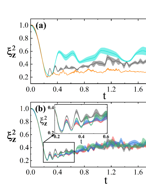
Figure 3: $(a)$ Mean evolution for 30 samples of the spin squeezing parameter with shaded error zone for different frequency of applying control pulses, control time interval $[0,2]$ is evenly divided into the number of segments at which the square pulse sequence with amplitude 2 ($\Omega(t)=2,0,-2$) is applied. We should confirm that each of the 30 samples is the one with smallest $\xi_{Z}^{2}$ among 600 epochs. It is reasonable since in practical scenarios, one choose the best control sequence in experiments. This results in the fluctuation error value contracting at time t=2. $(b)$ Evolution of the spin squeezing parameter for different number of control actions when the number of segments is 40: $\{\Omega(t)\}$=$\{(2,~{}0,~{}-2)|~{}actions=3\}$, $\{(2,~{}1~{},0,~{}-1,~{}-2)|~{}actions=5\}$, $\{(2,~{}1.34,~{}0.66,~{}0,~{}-0.66,~{}-1.34,~{}-2)|~{}actions=7\}$, $\{(2,~{}1.5,~{}1,~{}0.5,~{}0,~{}-0.5,~{}-1,~{}-1.5,~{}-2)|~{}actions=9\}$. The other parameters are same to those in Fig. 2 $(a)$.

Fig. 2 (d) presents the evolution of the spin squeezing parameter obtained by using RL-designed $\Omega(t)$: $\xi_{Z,RL}^{2}$, constant control field $\Omega(t)=-2$: $\xi_{Z,Con}^{2}$, and the optimized $\xi_{\perp,RL}^{2}$, with the minimal value at the final control time $t=2$ among the 600 epochs. The comparison clearly demonstrates a significantly enhanced performance of the reinforcement-learning-based control approach as opposed to the constant control scenario under the same parameter settings. And we employ the trace of the square of the system state $\rho(t)$: $Tr[\rho^{2}(t)]$, as an indicator for mixing of a quantum state. The degree of mixing of the state under RL control tend to be more deeply compared to $\Omega(t)=-2$. The optimal squeezing angle $\varphi\rightarrow\pi/2$, i.e., converges to z-component, which can be seen in Fig. 2 $(e_{1})$. The linear terms $\Omega_{x}(t)\hat{J}_{x}$ rotating of the redistributed fluctuation, combined with the twisting effect of $\hat{J}_{z}^{2}$, spin squeezed state is generated and maintained. The square wave control sequence corresponding to the RL control result in Fig. 2 (d) is depicted in Fig. 2 $(e_{2})$. Furthermore, Fig. 2 (f) utilizes the Husimi function and Wigner function to visualize the initial coherent spin state and final spin squeezed state at the time $t=2$. Nonclassical states are characterized by the twisted distribution in the Husimi function 8PR50989 ; 9PRA475138 and the asymmetry in the polar plot of the Wigner function PRA604034 ; PRL117180401 . This provides insight into the evolution of the quantum state under the control protocol.

We conjecture that the temporal application frequency of pulse impacts the outcomes of the control. To investigate the evolution of the squeezing parameter versus different application frequencies, we discretize the temporal interval [0, 2] into different number of segments, the more segments, the more frequently of applying the pulses. It can be seen in Fig. 3(a), with increasing of the segments, the squeezing parameter is depressed more stationary and lower. Even more, with increasing of the control pulses, the variance of the squeezing parameter is also depressed more obviously. Straightforwardly, there is a contradiction between the control performance and operation difficulty. One may conjecture the number of control actions may also influences the control performance. However, as shown in Fig. 3(b), there is no obvious advantage for more control actions with the same maximum control amplitude in this control.

It is pertinent to ask the applicability of the proposed scheme to collective spin models with different total spin numbers ($N=2J$). To address this concern, FIG. 4 ($a$) illustrates the control results for collective spin systems with different $N$. The result reveals that the squeezing parameter reaches lower values as $N$ increases within the same time interval. This observation suggests that an enlarged ensemble of entangled spins enhances the precision for quantum metrology. Furthermore, an examination of the subgraph discloses a convergence towards parallelism among the trajectories corresponding to different $N$, indicating an emergence of scaling behavior.

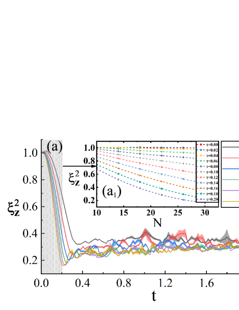
Figure 4: Average evolution for 30 samples of the spin squeezing parameter with error zone for different size of the collective spin system $N=2J$ under 3-action ($\Omega(t)=2,0,-2$) control. The samples are picked in the same manner as those shown in Fig. 3 $(a)$. The subgraph shows the squeezing parameter in the scaled time interval $t=0\sim 0.2$, picked from the shaded area on the left in the graph, for the collective spin system of different size. Same color is shared with the same $N$. The other parameters are same to those in Fig. 2 $(a)$.

In the system under consideration, energy dissipation concurrent with decoherence interplays with the applied coherent pulses which impedes the quantum system decay to the ground state. Consequently, the plateau in the squeezing parameter can be attributed to a dynamical equilibrium between these two conflicting processes.

In the previous results, the environmental temperature was assumed to be zero. To investigate the robustness of the proposed control scheme, it is necessary to check the influence of a finite temperature on the system dynamics. Since the temperature is positively correlated with the average number of thermal excitations of the reservoir, denoted as $n_{th}$. It reflects the strength of the decoherence. Fig. 5 illustrates that an incremental rise in thermal excitation of the surrounding reservoir progressively impairs the efficacy of the control scheme from the view of degree of squeezing and the control variance.

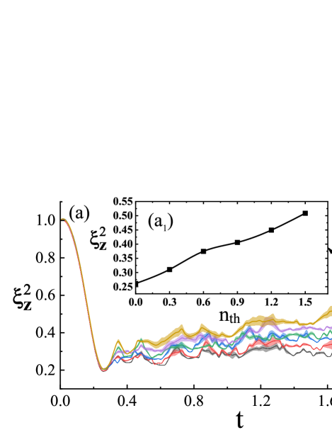
Figure 5: The average evolution of 30 squeezing parameter with error zone for different thermal excitations of the reservoir $n_{th}=\frac{1}{\exp(\hbar\omega/k_{B}T)-1}$, the average number of photons for a mode with frequency $\omega$ in the reservoir. The samples are picked in the same manner as those shown in Fig. 3 $(a)$. The subgraph shows the squeezing parameter versus average thermal excitations at the scaled time $t=2$. The other parameters are same to those in Fig. 2 $(a)$.

VII discussion

The interferometer operations are collectively acting on all particles identically. In the large $N$ (the number of particles) limit, this model can also be mapped to the bosonic model by the Holstein-Primakoff transformation: $\hat{J}_{z}=N/2-\hat{c}^{\dagger}\hat{c}\simeq N/2$ and $\hat{J}_{+}=(N-\hat{c}^{\dagger}\hat{c})^{1/2}\hat{c}\simeq\sqrt{N}\,\hat{c}$, where $\hat{c}$ ($\hat{c}^{\dagger}$) is a bosonic annihilation (creation) operator 68PR581098 . These maps between the collective spin model and the bosonic partners hint we may apply the control scheme on such quantum systems.

A control scheme is proposed in this study, wherein elements within the scheme can be replaced by modules possessing equivalent functions. Several candidate modules capable of substituting the reinforcement learning agent have been identified and evaluated. For example, the State-Action-Reward-State-Action algorithm 61CS2500611 , Deep Deterministic Policy Gradient 64PMLR387395 , Asynchronous Advantage Actor-Critic 66PMLR19281937 , Dueling Network 37arXiv151106581 and so on.

RL provides a tool to optimize dynamical process, i.e., the evolution of the quantum state. The optimal criteria various as certain quantum states or expectations of operators. The principle using this scheme is the system evolves or changes under certain mapping rules. And the optimal module just finds the road to a goal more efficiently. After all, machine learning learns the patterns or mappings based on statistical distribution.

VIII conclusion

In conclusion, we have proposed a reinforcement-learning based control strategy for the generation of non-classical collective spin states within an open environment. The machine can design a suite of control sequences to prepare spin squeezed states accompanied by entanglement. Larger frequency of application of the pulses enhances the efficacy of the control protocol. However more choice of actions do not contributes to the control outcomes obviously. The scalability of this framework is demonstrated, facilitating its applicability to larger systems wherein. Notably, thermal excitations progressively undermine the control performance. The versatility of this scheme is underlined by the potential for substituting the reinforcement learning agent with alternative optimization modules, as well as extending the control paradigm to other quantum systems which can provide quantum resources.

References

- (1) J. Ma, X. G. Wang, C. P. Sun, and F. Nori, Quantum spin squeezing, Physics Reports 509, 89 (2011).
- (2) L. Pezzè, A. Smerzi, M. K. Oberthaler, R. Schmied, and P. Treutlein, Quantum metrology with nonclassical states of atomic ensembles, Rev. Mod. Phys. 90, 035005 (2018).
- (3) D. J. Wineland, J. J. Bollinger, W. M. Itano, F. L. Moore, and D. J. Heinzen, Spin squeezing and reduced quantum noise in spectroscopy, Phys. Rev. A 46, R6797 (1992).
- (4) D. J. Wineland, J. J. Bollinger, W. M. Itano, and D. J. Heinzen, Squeezed atomic states and projection noise in spectroscopy, Phys. Rev. A 50, 67 (1994).
- (5) R. J. Sewell, M. Koschorreck, M. Napolitano, B. Dubost, N. Behbood, and M. W. Mitchell, Magnetic Sensitivity Beyond the Projection Noise Limit by Spin Squeezing, Phys. Rev. Lett. 109, 253605 (2012).
- (6) A. D. Ludlow, M. M. Boyd, J. Ye, E. Peik, and P. O. Schmidt, Optical atomic clocks, Rev. Mod. Phys. 87, 637 (2015).
- (7) L. Pezzé, and Augusto Smerzi, Entanglement, Nonlinear Dynamics, and the Heisenberg Limit, Phys. Rev. Lett. 102, 100401 (2009).
- (8) M. Kitagawa and M. Ueda, Squeezed spin states, Phys. Rev. A 47, 5138 (1993).
- (9) A. Kuzmich, N. P. Bigelow, and L. Mandel, Atomic quantum non-demolition measurements and squeezing, Europhys. Lett. 42, 481 (1998).
- (10) L. M. Duan, A. Sørensen, J. I. Cirac, and P. Zoller, Squeezing and Entanglement of Atomic Beams, Phys. Rev. Lett. 85, 3991 (2000).
- (11) C. K. Law, H. T. Ng, and P. T. Leung, Coherent control of spin squeezing, Phys. Rev. A 63, 055601 (2001).
- (12) K. P. Murphy, Machine learning: a probabilistic perspective (MIT Press, 2012).
- (13) R. S. Sutton and A. G. Barto, Reinforcement learning: An introduction (MIT press, 2018).
- (14) T. Fsel, P. Tighineanu, T. Weiss, and F. Marquardt, Reinforcement Learning with Neural Networks for Quantum Feedback, Phys. Rev. X 8, 031084 (2018).
- (15) V. Dunjko, and H. J. Briegel, Machine learning and artificial intelligence in the quantum domain: a review of recent progress, Reports on Progress in Physics 81, 074001 (2018).
- (16) H. Xu, J. Li, L. Liu, Y. Wang, H. Yuan, and X. Wang, Generalizable control for quantum parameter estimation through reinforcement learning, NPJ Quantum Information 5, 82 (2019).
- (17) S. Grivopoulos, and B. Bamieh, Lyapunov-based control of quantum systems, In Proceedings of the 42nd IEEE conference on decision and control 1, 434 (2003).
- (18) M. Mirrahimi, P. Rouchon, and G. Turinici, Lyapunov control of bilinear Schrdinger equations, Automatica 41, 1987 (2005).
- (19) R. V. Handel, J. K. Stockton, and H. Mabuchi, Feedback control of quantum state reduction, IEEE Trans. Automat. Control 50, 768 (2005).
- (20) X. X. Yi, S. L. Wu, C. F. Wu, X. L. Feng, and C. H. Oh, Time-delay effects and simplified control fields in quantum Lyapunov control, J. Phys. B: At. Mol. Opt. Phys. 44, 195503 (2011).
- (21) S. C. Hou, L. C. Wang, and X. X. Yi, Realization of quantum gates by Lyapunov control, Physics Letters A 378, 699 (2014).
- (22) V. Mnih, K. Kavukcuoglu, D. Silver, A. A. Rusu, J. Veness, M. G. Bellemare, A. Graves, M. Riedmiller, A. K. Fidjeland, G. Ostrovski, S. Petersen, C. Beattie, A. Sadik, I. Antonoglou, H. King, D. Kumaran, D. Wierstra, S. Legg, and D. Hassabis, Human-level control through deep reinforcement learning, Nature 518, 529 (2015).
- (23) R. Bellman, On the theory of dynamic programming, PNAS 38, 716 (1952).
- (24) Y. LeCun, Y. Bengio, and G. Hinton, Deep learning, nature 521, 436 (2015).
- (25) I. Goodfellow, Y. Bengio, and A. Courville, Deep Learning (MIT Press,2016).
- (26) M. Hessel, J. Modayil, H. v. Hasselt, T. Schaul, G. Ostrovski, W. Dabney, D. Horgan, B. Piot, M. Azar, and D. Silver, Rainbow: Combining Improvements in Deep Reinforcement Learning, In Proceedings of the 30nd AAAI Conference on Artificial Intelligence 32, 1 (2018).
- (27) G. A. Rummery, and M. Niranjan, On-Line Q-Learning Using Connectionist Systems, Department of Engineering (University of Cambridge, 1994).
- (28) F. S. Melo, Convergence of Q-learning: a Simple Proof, Tech. Rep (2001).
- (29) D. Silver, G. Lever, N. Heess, T. Degris, D. Wierstra, and M. Riedmiller, Deterministic Policy Gradient Algorithms, PMLR 32, 387(2014).
- (30) T. P. Lillicrap, J. J. Hunt, A. Pritzel, N. Heess, T. Erez, Y. Tassa, D. Silver, D. Wierstra, Continuous Control with Deep Reinforcement Learning, arXiv: 1509.02971 (2019).
- (31) V. Mnih, A. P. Badia, M. Mirza, A. Graves, T. Harley, T. P. Lillicrap, D. Silver, K. Kavukcuoglu, Asynchronous Methods for Deep Reinforcement Learning, International Conference on Machine Learning, PMLR 48 1928 (2016).
- (32) Z. Wang, T. Schaul, M. Hessel, H. v. Hasselt, M. Lanctot, and N. d. Freitas, Dueling Network Architectures for Deep Reinforcement Learning, PMLR 48, 1995 (2016).
- (33) F. T. Arecchi, E. Courtens, R. Gilmore, and H. Thomas, Atomic Coherent States in Quantum Optics, Phys. Rev. A 6, 2211 (1972).
- (34) L. G. Biederharn, and J. C. Louck, Angular Momentum in Quantum Physics: Theory and Applications (Addison-Wesley, Reading, MA, 1981).
- (35) L. Song, X. Wang, D. Yan, Z. Zong, Spin squeezing properties in the quantum kicked top model, J. Phys. B: At. Mol. Opt. Phys. 39 559(2006).
- (36) A. S. Sørensen, and K. Mølmer, Entanglement and Extreme Spin Squeezing, Phys. Rev. Lett. 86, 4431 (2001).
- (37) G. Tóth, Multipartite entanglement and high- precision metrology, Phys. Rev. A 85, 022322 (2012).
- (38) V. Giovannetti, S. Lloyd, and L. Maccone, Quantum-Enhanced Measurements: Beating the Standard Quantum Limit, Science, 306, 1330 (2004).
- (39) C. W. Helstrom, Quantum detection and estimation theory, J. Stat. Phys. 1, 231(1969).
- (40) H. Strobel, W. Muessel, D. Linnemann, T. Zibold, D. B. Hume, L. Pezze, A. Smerzi, and M. K. Oberthaler, Fisher information and entanglement of non-Gaussian spin states, Science 345, 424 (2014).
- (41) C. W. Helstrom, Minimum mean-squared error of estimates in quantum statistics, Phys. Lett. A 25, 101 (1967).
- (42) S. L. Braunstein and C. M. Caves, Statistical distance and the geometry of quantum states, Phys. Rev. Lett. 72, 3439 (1994).
- (43) Y. M. Zhang, X. W. Li, W. Yang, and G. R. Jin, Quantum Fisher information of entangled coherent states in the presence of photon loss, Phys. Rev. A 88, 043832 (2013).
- (44) Liu J, Jing X-X and Wang X Quantum metrology with unitary parametrization processes Sci. Rep. 5, 8565 (2015).
- (45) P. Hyllus, W. Laskowski, R. Krischek, C. Schwemmer, W. Wieczorek, H. Weinfurter, L. Pezzé, and A. Smerzi, Fisher information and multiparticle entanglement, Phys. Rev. A 85, 022321 (2012).
- (46) A. Sørensen, L. M. Duan, J. L. Cirac, and P. Zoller, Many-particle entanglement with Bose-Einstein condensates, Nature (London) 409, 63 (2001).
- (47) P. J. Huber. Robust Estimation of a Location Parameter, Annals of Mathematical Statistics 35, 73(1964).
- (48) I. Loshchilov, and F. Hutter, Decoupled Weight Decay Regularization, https://arxiv.org/abs/1711.05101.
- (49) M. G. Benedict, and A. Czirjk, Wigner functions, squeezing properties, and slow decoherence of a mesoscopic superposition of two-level atoms, Phys. Rev. A 60, 4034(1999).
- (50) T. Tilma, M. J. Everitt, J. H. Samson, W. J. Munro, and K. Nemoto, Wigner Functions for Arbitrary Quantum Systems, Phys. Rev. Lett. 117, 180401(2016).
- (51) T. Holstein and H. Primakoff, Field Dependence of the Intrinsic Domain Magnetization of a Ferromagnet, Phys. Rev. 58, 1098 (1940).