Probability that $n$ points are in convex position in a regular $\kappa$-gon :
Asymptotic results.

Abstract

Let $\mathbb{P}_{\kappa}(n)$ be the probability that $n$ points $z_{1},\ldots,z_{n}$ picked uniformly and independently in $\mathfrak{C}_{\kappa}$, a regular $\kappa$-gon with area $1$, are in convex position, that is, form the vertex set of a convex polygon. In this paper, we give an equivalent of $\mathbb{P}_{\kappa}(n)$ for all $\kappa\geq 3$, which improves on a famous result of Bárány [3]. A second aim of the paper is to establish a limit theorem which describes the fluctuations around the limit shape of a $n$-tuple of points in convex position when $n\to+\infty$. Finally, we give an algorithm asymptotically exact for the random generation of $z_{1},\ldots,z_{n}$, conditioned to be in convex position in $\mathfrak{C}_{\kappa}$.

Mathematics Subject Classification (2020):

Primary 52A22; 60D05

Keywords:

Random convex chains, random polygon, Sylvester’s problem, stochastic geometry

1 Introduction

Let $\mathfrak{C}_{\kappa}$ be the regular $\kappa$-gon with area $1$ positioned on the $X$-axis, as represented in Figure 1, $r_{\kappa}=\left(4\tan\left(\frac{\pi}{\kappa}\right)/\kappa\right)^{1/2}$ be its side length, and $\theta_{\kappa}=\frac{(\kappa-2)\pi}{\kappa}$ be the interior angle between two consecutive sides.

For any compact convex domain $K$ of area 1 in $\mathbb{R}^{2}$ with non empty interior and for any $n\in\mathbb{N}$, we let $\mathbb{U}_{K}^{(n)}$ denote the law of a $n$-tuple $\mathbf{z}[n]:=(\mathbf{z}_{1},\cdots,\mathbf{z}_{n})$, where the $\mathbf{z}_{i}$ are independent and identically distributed (i.i.d.) and uniform in $K$.

In the special case $K=\mathfrak{C}_{\kappa}$, we write for short $\mathbb{U}^{(n)}_{\kappa}:=\mathbb{U}^{(n)}_{\mathfrak{C}_{\kappa}}$.

Figure 1: $\mathfrak{C}_{7}$

A $n$-tuple of points $z[n]\in(\mathbb{R}^{2})^{n}$ is said to be in convex position if $\{z_{1},\cdots,z_{n}\}$ is the vertex set of a convex polygon, which we will refer to as the $z[n]$-gone; the set of such $n$-tuples ${z}[n]$ is denoted by $\mathcal{Z}_{n}$. Hence

$$\mathbb{P}_{K}(n):=\mathbb{P}\left(\mathbf{z}[n]\in\mathcal{Z}_{n}\right)=\mathbb{U}^{(n)}_{K}(\mathcal{Z}_{n}),$$

is the probability that $n$ i.i.d. random points $\mathbf{z}[n]$ taken uniformly in $K$, are in convex position, and

$$\mathbb{P}_{\kappa}(n):=\mathbb{P}_{\mathfrak{C}_{\kappa}}(n),$$

is the corresponding probability in the regular $\kappa$-gon.

The aim of this paper is threefold. First, we give an equivalent of $\mathbb{P}_{\kappa}(n)$ (see 1.1 below), then we describe the fluctuations of a ${z}[n]$-gon under $\mathbb{U}^{(n)}_{\kappa}$ conditioned to be in convex position (5.2), and we conclude by provinding an algorithm to sample such a $n$-tuple ${z}[n]$ (Section 6). One of the main contributions of this paper is thus the following theorem :

Theorem 1.1.

Let $\kappa\geq 3$ be an integer. We have

$$\mathbb{P}_{\kappa}(n)\underset{n\to+\infty}{\sim}C_{\kappa}\cdot\frac{e^{2n}}{4^{n}}\frac{\kappa^{3n}r_{\kappa}^{2n}\sin(\theta_{\kappa})^{n}}{n^{2n+\kappa/2}},$$

where

$$C_{\kappa}=\frac{1}{\pi^{\kappa/2}\sqrt{\mathbb{d}_{\kappa}}}\frac{\sqrt{\kappa}^{\kappa+1}}{4^{\kappa}(1+\cos(\theta_{\kappa}))^{\kappa}},$$

and

$$\mathbb{d}_{\kappa}=\frac{\kappa}{3\cdot 2^{\kappa}}\left(2(-1)^{\kappa-1}+(2-\sqrt{3})^{\kappa}+(2+\sqrt{3})^{\kappa}\right).$$

Theorem 1.1 actually refines a famous result of Bárány [3] in the case of $\kappa$-gons (note however, that Bárány’s result holds under weaker hypothesis):

Theorem 1.2.

[3] For any compact convex set $K$ of area 1 with non empty interior,

$$\lim_{n\to+\infty}n^{2}\left(\mathbb{P}_{K}(n)\right)^{\frac{1}{n}}=\frac{1}{4}e^{2}\operatorname{AP}^{*}(K)^{3},$$

where $\operatorname{AP}^{*}(K)$ is the supremum of the affine perimeters of all convex sets $S\subset K.$

The definition of the affine perimeter will be recalled in A.1; we send the interested reader to [2] for additional details (in Figure 2, in the $\kappa$-gon case, we represent the supremum of affine perimeters in terms of the area of some hatched domains).

As will be shown in A.5, we have

$$\operatorname{AP}^{*}(\mathfrak{C}_{\kappa})=\kappa\left(r_{\kappa}^{2}\sin(\theta_{\kappa})\right)^{1/3},$$

so that, one can check that in the particular $\kappa$-gon case, 1.1 is compatible and more precise than 1.2.

       

Figure 2: For each case $\kappa=3$, 4 and 6, the inner curve drawn in red delimits a convex domain ${\sf Dom}(\mathfrak{C}_{\kappa})$ inside $\mathfrak{C}_{\kappa}$. The red curve represents the limit shape of a $\mathbf{z}[n]$-gone taken under $\mathbb{U}^{(n)}_{\kappa}$, conditioned to be in convex position, when $n\to+\infty$. The curve can be drawn as follows: add the midpoint of the sides of the initial $\kappa$-gone, and between two consecutive midpoints, add the arc of parabola which is tangent to the sides and incident to these inner points. The sum of the hatched areas corresponds to the supremum of affine perimeters (see an explanation in Appendix, A.5).

The value of $\mathbb{P}_{K}(n)$ has been widely studied since the 19th century, and for a large variety of convex sets $K$, not just regular ones. Sylvester [22] initiated the reflection on this matter looking at the probability that four points chosen at random in the plane were in convex position. Though Sylvester’s question was ill-posed, it matured in its later formulation into the study of $\mathbb{P}_{K}(4)$, for any convex shape $K$ of area 1 (see Pfiefer [19] for historical notes). In 1917, Blaschke [5] determined the convex domain $K$ that maximizes or minimizes the probability $\mathbb{P}_{K}(4)$ (on the set of nonflat compact convex domains of $\mathbb{R}^{2}$) by proving that the lower bound is achieved when $K=\triangle$ is a triangle, and the upper bound when $K=\bigcirc$ is a disk, namely

$$\frac{2}{3}=\mathbb{P}_{\triangle}(4)\leq\mathbb{P}_{K}(4)\leq\mathbb{P}_{\bigcirc}(4)=1-\frac{35}{12\pi^{2}}.$$

In the same direction, Marckert and Rahmani [17] proved in 2021 that

$$\frac{11}{36}=\mathbb{P}_{\triangle}(5)\leq\mathbb{P}_{K}(5)\leq\mathbb{P}_{\bigcirc}(5)=1-\frac{305}{48\pi^{2}}.$$

This question can be generalized to different values of $n$, and other dimensions. To this day, the conjecture in dimension $2$, for all $n\geq 3$:

$$\mathbb{P}_{\triangle}(n)\leq\mathbb{P}_{K}(n)\leq\mathbb{P}_{\bigcirc}(n),$$

remains open. Yet, the value $\mathbb{P}_{\bigcirc}(n)$ is computable for all $n\geq 3$ since 2017 thanks to Marckert’s algebraic formula [16] in the disk case. Note also that Hilhorst, Calka and Schehr [12] managed in 2008 to derive an asymptotic expansion of $\log{\mathbb{P}_{\bigcirc}(n)}$.

In the case of regular convex polygons, exact formulas are rare but Valtr [23] proved in 1995 that for a parallelogram $K=\square$

$$\mathbb{P}_{4}(n)=\mathbb{P}_{\Box}(n)=\frac{1}{(n!)^{2}}{2n-2\choose n-1}^{2}\underset{n\to+\infty}{\sim}\frac{1}{\pi^{2}2^{5}}\frac{4^{2n}e^{2n}}{n^{2n+2}}$$

and in 1996 when $K$ is a triangle [24]

$$\mathbb{P}_{3}(n)=\mathbb{P}_{\triangle}(n)=\frac{2^{n}(3n-3)!}{(2n)!((n-1)!)^{3}}\underset{n\to+\infty}{\sim}\frac{\sqrt{3}}{4}\frac{1}{\pi^{3/2}3^{3}}\frac{3^{3n}e^{2n}}{2^{n}n^{2n+3/2}}.$$

The equivalents given at the right-hand-side are of course consistent with Theorem 1.1. Note however that our method will allow us to recover Valtr’s formulas in Appendix B (our approach avoids discretization arguments, but it largely relies on Valtr’s ideas.)

In dimension $d\geq 3$, if $\triangle^{d}$ and $\bigcirc^{d}$ denote respectively a simplex and an ellipsoïde of volume 1, the following generalization of Sylvester’s question

$$\mathbb{P}_{\triangle^{d}}(d+2)\leq\mathbb{P}_{K}(d+2)\leq\mathbb{P}_{\bigcirc^{d}}(d+2),$$

for any convex domain $K\subset\mathbb{R}^{d}$ of volume $1$, is a conjecture that remains to be proven (though the right inequality is known as a generalization of Blaschke’s proof in dimension 2). For a comprehensive overview of these matters, we refer to Schneider [20].

Canonical ordering of $z[n]$-gones.

An element of $z[n]\in\mathcal{Z}_{n}$ (in convex position) is said to be in convex canonical order if it satisfies the following conditions (see Figure 3):
$\bullet$ If $(x_{i},y_{i})$ is the coordinates of $z_{i}$ in $\mathbb{R}^{2}$, $y_{1}\leq y_{i}$ for all $i$ (that is, $z_{1}$ has the smallest $y$-component), and among those having the minimal $y$ component, it has the smallest $x$ component.
$\bullet$ The sequence $(\arg(z_{i+1}-z_{i}),1\leq i\leq n-1)$ is non-decreasing in $[0,2\pi]$.

Figure 3: Some $z[n]$ in $\mathcal{C}_{7}(n)$

We denote by $\overset{\curvearrowleft}{\mathcal{Z}}_{n}$ the subset of $\mathcal{Z}_{n}$ of $n$-tuples of points ${z}[n]$ in convex canonical order. The symmetric group ${\cal S}_{n}$ acts transitively on $\mathcal{Z}_{n}$ by relabelling the vertex indices; each orbit contains a unique element of $\overset{\curvearrowleft}{\mathcal{Z}}_{n}$. We put $\mathcal{C}_{\kappa}(n)=\mathcal{Z}_{n}\cap(\mathfrak{C}_{\kappa})^{n}$ and $\overset{\curvearrowleft}{\mathcal{C}_{\kappa}}(n)=\overset{\curvearrowleft}{\mathcal{Z}}_{n}\cap(\mathfrak{C}_{\kappa})^{n}$.

Since $\mathbf{z}[n]$ is picked according to the uniform distribution on $(\mathfrak{C}_{\kappa})^{n}$, and since this measure is the Lebesgue measure $\mathsf{Leb}$ on this set, we have

$$\mathbb{P}_{\kappa}(n)=\mathsf{Leb}(\mathcal{C}_{\kappa}(n))=n!\leavevmode\nobreak\ \mathsf{Leb}(\overset{\curvearrowleft}{\mathcal{C}_{\kappa}}(n)).$$

In the sequel, we will abandon $\mathcal{C}_{\kappa}(n)$ and work mainly in $\overset{\curvearrowleft}{\mathcal{C}_{\kappa}}(n)$ for the elements of this set are easier to parameterize. The argument we will coin in order to compute $\mathsf{Leb}(\overset{\curvearrowleft}{\mathcal{C}_{\kappa}}(n))$ is mainly deterministic, and we will not really use random variables in the analysis, even if everything could be rewritten in terms of these latters (but the proof appears way heavier to us in these terms).

Notation 1.3.

From now on, we denote by $\overset{\curvearrowleft}{\mathbb{Q}}^{(n)}_{K}$, the law of a $n$-tuple of points taken under $\mathbb{U}^{(n)}_{\kappa}$, conditioned to be in $\overset{\curvearrowleft}{\mathcal{C}_{\kappa}}(n)$, and denote for short $\overset{\curvearrowleft}{\mathbb{Q}}^{(n)}_{\kappa}=\overset{\curvearrowleft}{\mathbb{Q}}^{(n)}_{\mathfrak{C}_{\kappa}}$, that is:

$$\mathrm{d}\overset{\curvearrowleft}{\mathbb{Q}}^{(n)}_{\kappa}(z[n])=\frac{n!}{\mathbb{P}_{\kappa}(n)}\mathbb{1}_{z[n]\in\overset{\curvearrowleft}{\mathcal{C}_{\kappa}}(n)}\mathrm{d}z_{1}\ldots\mathrm{d}z_{n}.$$

This formula represents the measure, but it is hardly exploitable for further computations; we will thus need an alternative geometrical understanding of $\overset{\curvearrowleft}{\mathcal{C}_{\kappa}}(n)$, which was inspired by Valtr’s papers.

Limit shape.

Bárány [2] proved in 1999 that the convex hull of a $n$-tuple $\mathbf{z}[n]$ taken under $\overset{\curvearrowleft}{\mathbb{Q}}^{(n)}_{\kappa}$ converges in distribution for the Hausdorff topology to an explicit deterministic domain ${\sf Dom}(K)$. In the case of the $\kappa$-gon, we will explain in Figure 17 and in A.2 how ${\sf Dom}(\mathfrak{C}_{\kappa})$ is determined using $\mathfrak{C}_{\kappa}$’s inner symmetries (a first look at ${\sf Dom}(\mathfrak{C}_{\kappa})$ is possible in Figure 2).

Denote by $d_{H}$ the Hausdorff distance on the set of compact sets of $\mathbb{R}^{2}$, and for any tuple ${z}[n]\in(\mathbb{R}^{2})^{n}$, let ${\sf CH}({z}[n])$ be its convex hull. In the second main contribution of this paper, we detail the fluctuations of the $\mathbf{z}[n]$-gone under $\overset{\curvearrowleft}{\mathbb{Q}}^{(n)}_{\kappa}$ around its limit ${\sf Dom}(\mathfrak{C}_{\kappa})$:

Theorem 1.4.

Let $\kappa\geq 3$ be fixed, and let $\mathbf{z}[n]$ be taken under $\overset{\curvearrowleft}{\mathbb{Q}}^{(n)}_{\kappa}$. When $n\to+\infty$, we have

$$n^{1/2}d_{H}\left({\sf CH}(\mathbf{z}[n]),{\sf Dom}(\mathfrak{C}_{\kappa})\right)\xrightarrow[n]{(d)}\Delta$$

where $\Delta$ is a non trivial random variable.

This theorem will appear to be a consequence of the convergence of the fluctuations of $\mathbf{z}[n]$-gone in distribution (at scale $1/\sqrt{n}$) in a functional space, which is stated in 5.2. However, we renounce to state at this point this theorem since it would require to introduce too much material to do so, and then, we postpone this work to Section 5.

Nonetheless, we disclose an element of the proof: the main idea is to partition each ${z}[n]$-gone of $\overset{\curvearrowleft}{\mathcal{C}_{\kappa}}(n)$ into $\kappa$ suitable convex chains, one per corner of the initial polygon $\mathfrak{C}_{\kappa}$. Each of the convex chains will be shown to converge separately towards the arc of parabola associated with the corresponding "corner" of $\mathfrak{C}_{\kappa}$, as introduced in Figure 2.

The convergence results stated in 5.2 are reminiscent of the limit theorems concerning lattice convex polygons: in this model, an integer $n$ is given, and a convex (lattice) polygon is a convex polygon contained in the square $[-n,n]^{2}$ and having vertices with integer coordinates (and any number of sides). Vershik asked whether it was possible to determine the number and typical shape of convex lattice polygons contained in $[-n,n]^{2}.$ Three different solutions were brought to light by Bárány [1], Vershik [25] and Sinai [21] in 1994:

A convex lattice convex polygons can be decomposed naturally in 4 parts (delimited by the extreme points in the North/East/South/West directions), which delimitate 4 “polygonal convex lines” between them. It is therefore natural to investigate the behaviour of these chains, that can be considered, in a first approximation, as convex chains going from $(0,0)$ to $(n,n)$ in the square $[0,n]^{2}$ (up to rotations/translations). For these chains, they proved that when $n\to+\infty,$

1. the number of these convex polygonal lines is $\exp(3(\xi(3)/\xi(2))^{1/3}n^{2/3}+o(n^{2/3}))$,

2. the random number of vertices in such a chain is concentrated around $\left(\xi(3)^{2}/\xi(2)\right)^{-1/3}n^{2/3}$,

3. the limit shape of such a chain, normalized in both direction by $n$, is an arc of parabola.

These results were refined by Bureaux, Enriquez [9] in 2016, and generalized in larger dimensions by Bárány, Bureaux, Lund [10] in 2018, as well as Buffière [8] for zonotopes in 2023.

On a related topic, the paper by Bodini, Jacquot, Duchon and Mutafchiev [6] gives a characterization of digitally convex polyominoes using combinatorics on words.

Random generation of a $\mathbf{z}[n]$-gone under $\overset{\curvearrowleft}{\mathbb{Q}}^{(n)}_{\kappa}$.

The naive way of sampling a $\mathbf{z}[n]$-gone under $\overset{\curvearrowleft}{\mathbb{Q}}^{(n)}_{\kappa}$ consists in rejection sampling, i.e. sampling points under $\mathbb{U}_{n}^{(\kappa)}$ until they are in $\overset{\curvearrowleft}{\mathcal{C}_{\kappa}}(n)$ (or in $\mathcal{C}_{\kappa}(n)$). This algorithm works fine for small values of $n$ but as $n$ grows, computation times are not acceptable anymore (by Theorem 1.1, the probability of success is less than $\frac{k^{n}}{n^{2n}}$ for some constant $k$). In particular, the limit shape theorem proven by Bárány cannot be observed empirically with such a method.

A comprehensive understanding of the distribution $\overset{\curvearrowleft}{\mathbb{Q}}^{(n)}_{\kappa}$ will allow us to determine another distribution $\overset{\curvearrowleft}{\mathbb{O}}^{(n)}_{\kappa}$, for which we have an exact sampling algorithm (called $\kappa$-sampling and defined in Section 6) that behaves asymptotically like $\overset{\curvearrowleft}{\mathbb{Q}}^{(n)}_{\kappa}$, meaning $d_{V}(\overset{\curvearrowleft}{\mathbb{Q}}^{(n)}_{\kappa},\overset{\curvearrowleft}{\mathbb{O}}^{(n)}_{\kappa})\underset{n\to+\infty}{\longrightarrow}0$ where $d_{V}$ is the total variation distance. The distribution $\overset{\curvearrowleft}{\mathbb{O}}^{(n)}_{\kappa}$ is defined in Section 3, and can be viewed as $\overset{\curvearrowleft}{\mathbb{Q}}^{(n)}_{\kappa}$ conditioned to satisfy a property which occurs with probability going to 1. This algorithm can be then seen as an algorithm asymptotically exact (in $n$, for $\kappa$ fixed), for the sampling under $\overset{\curvearrowleft}{\mathbb{Q}}^{(n)}_{\kappa}$.

Theorem 1.5.

The algorithm of $\kappa$-sampling samples a $n$-tuple of points under $\overset{\curvearrowleft}{\mathbb{O}}^{(n)}_{\kappa}$ with a complexity of $\mathcal{O}\left(n^{\kappa/2+1}\kappa\log(\kappa)\right).$

Contents of the paper.

In the second section of this paper, we analyze the properties of a $n$-tuple ${z}[n]\in\overset{\curvearrowleft}{\mathcal{C}_{\kappa}}(n)$ in the light of a new geometric description. We derive in Section 3 the distribution of the important variables of this geometric scheme, ouf of which we provide the proof of 1.1 in Section 4. Section 5 is dedicated to the proof of 1.4 and the understanding of the fluctuations of ${z}[n]$ around its limit. In Section 6, we provide the aforementioned algorithm of $\kappa$-sampling and some alternative (more efficient) versions in the cases $\kappa=3$ and 4. As for the appendices, the first is dedicated to some complementary proofs of the paper, and the second provides a new demonstration of Valtr’s formulas in the triangle and the parallelogram.

2 Geometrical aspects

Notation.

In the sequel, $\kappa\geq 3$ is considered to be fixed. The notation $\widebar{j}$ will stand for the integer $j$ in $\{1,\ldots,\kappa\}$ such that $\bar{j}-j\equiv 0\mod\kappa$ (so that this notation is a bit different from the usual modulo notation, since $\bar{\kappa}=\kappa$).

We start by the definition of the "Equiangular Circumscribed Polygon" $\mathsf{ECP}({z}[n])$ associated to ${z}[n]\in\overset{\curvearrowleft}{\mathcal{C}_{\kappa}}(n)$, any $n$-tuple of points in canonical convex order: as represented (in blue) on LABEL:fig2, this is the polygon equal to the intersection of all equiangular polygons whose sides are parallel one by one to those of $\mathfrak{C}_{\kappa}$, and which contain ${z}[n]$.

We now define some quantities that will somehow allow the description of ${z}[n]$ in term of its circumscribed polygon (see also LABEL:fig2).

The distance from the $j^{th}$ side of $\mathfrak{C}_{\kappa}$ to $z[n]$ is denoted by $\ell_{j}:=\ell_{j}({z}[n])$. The length of the side of $\mathsf{ECP}({z}[n])$ parallel to the X-axis is denoted by $c_{1}:=c_{1}({z}[n])$. Then, the consecutive side lengths of $\mathsf{ECP}({z}[n])$, sorted anticlockwise, are denoted by $c_{1},c_{2},\ldots,c_{\kappa}$, one or several $c_{i}$ being possibly zeroes.

Figure 4: On the left, in blue, $\mathsf{ECP}({z}[n])$ for a $n$-tuple taken in $\overset{\curvearrowleft}{\mathcal{C}_{7}}(n)$, with the distances $\ell[7]$ from the sides of $\mathfrak{C}_{7}$ to those of $\mathsf{ECP}(z[n]).$ The sides -which lengths are the tuple of values $c[7]$- of this latter polygon are colored in blue. On the right, a $6$-sides $\mathsf{ECP}({z}[n])$ in $\mathfrak{C}_{7}$. One of the sides is reduced to a point: this happens when three consecutives $\ell_{\widebar{j-1}},\ell_{j},\ell_{\widebar{j+1}}$ are defined on the same point $z_{i}$ in ${z}[n]$.

Remark 2.1.

If $\kappa=3$, the only possible internal polygons within $\mathfrak{C}_{3}$ are equilateral triangles. If $\kappa=4$, only rectangles are admitted. In both these cases, an internal polygon within $\mathfrak{C}_{\kappa}$ has exactly $\kappa$ sides. This is no longer true for $\kappa\geq 5$, as we may see on the right picture of LABEL:fig2. The number of "nonzero sides" of $\mathsf{ECP}({z}[n])$ is bounded above by $\kappa$, and below by 3 (in fact 4 for the $\kappa=4$ case, and it can technically be two, if all the points in ${z}[n]$ are aligned, but we can neglect this case).

Some properties of equiangular circumscribed polygons.

A moment thought allows to see that $\mathsf{ECP}({z}[n])$ is characterized by the $\kappa$-tuple of distances $\ell[\kappa]({z}[n]):=(\ell_{1}({z}[n]),\cdots,\ell_{\kappa}({z}[n]))$, and that, in turn, $\ell[\kappa]({z}[n])$ determines the side lengths of the $\mathsf{ECP}$, $c[\kappa]({z}[n])=(c_{1}({z}[n]),\cdots,c_{\kappa}({z}[n]))$.

Proposition 2.2.

Let $z[n]\in\overset{\curvearrowleft}{\mathcal{C}_{\kappa}}(n)$, and $c[\kappa]=c[\kappa](z[n]),\ell[\kappa]=\ell[\kappa](z[n]).$

• The $\ell[\kappa]$ and $c[\kappa]$ are related by the $\kappa$ equations

  $$c_{j}=r_{\kappa}-\mathfrak{cl}_{j}(\ell[\kappa]),\quad\forall j\in\{1,\ldots,\kappa\}.$$ (1)

  where for all $j\in\{1,\ldots,\kappa\}$, $\mathfrak{cl}_{j}(\ell[\kappa]):=\left(\ell_{\overline{j-1}}+\ell_{\overline{j+1}}+2\ell_{j}\cos(\theta_{\kappa})\right)/\sin(\theta_{\kappa})$ ($\mathfrak{cl}$ standing for "linear combination")

• The set $\mathcal{L}_{\kappa}=\ell[\kappa]\left(\overset{\curvearrowleft}{\mathcal{C}_{\kappa}}(n)\right)$ (of all possible vectors $\ell[\kappa]$) is the set of solutions $\ell[\kappa]$ to the inequations

  $$\mathfrak{cl}_{j}(\ell[\kappa])\leq r_{\kappa},\quad\forall j\in\{1,\ldots,\kappa\},$$

  together with the conditions $\ell_{j}\geq 0,j\in\{1,\ldots,\kappa\}.$

• The perimeter of the ${z}[n]$-gon satisfies

  $$\sum_{j=1}^{\kappa}c_{j}+\frac{2(1+\cos(\theta_{\kappa}))}{\sin(\theta_{\kappa})}\sum_{j=1}^{\kappa}\ell_{j}=\kappa r_{\kappa}.$$

Proof.

The formulas (1) may be deduced from routine computations on the angles and some proper applications of Thalès’ Theorem according to Figure 5 below. Now, $(ii)$ is a consequence of $(i)$ since for $\kappa\geq 3$, $c_{j}\geq 0$ and $\sin(\theta_{\kappa})>0$. To get $(iii)$, just sum all equations (1) for all values of $j$.

Figure 5: Characteristics of an internal polygon

∎

"Contact points".

For each ${z}[n]$ in $\overset{\curvearrowleft}{\mathcal{C}_{\kappa}}(n)$, each side of $\mathsf{ECP}({z}[n])$ contains at least one element of $\{z_{1},\cdots,z_{n}\}$. The $j^{th}$ "contact point" ${\sf cp}_{j}({z}[n])$ is the point of $\{z_{1},\cdots,z_{n}\}$, which is on the $j^{th}$ side of $\mathsf{ECP}({z}[n])$, and which is the smallest for the lexicographical order among those with this property (note that we will work with $n$-tuples $\mathbf{z}[n]$ of random variables, so that when $\mathbf{z}[n]$ is $\overset{\curvearrowleft}{\mathbb{Q}}^{(n)}_{\kappa}$-distributed, there is a single point of $\{\mathbf{z}_{1},\cdots,\mathbf{z}_{n}\}$ in the $j^{th}$ side of $\mathsf{ECP}(\mathbf{z}[n])$ with probability 1, so that the particular choice of the lexicographical order has no importance). However, ${\sf cp}_{j}={\sf cp}_{\widebar{j+1}}$ is possible, and has a positive probability for all $n\geq 1$.

Denote by $\mathsf{b}_{j}$ the intersection point between the $j^{th}$ and $\widebar{j+1}^{th}$ sides of $\mathsf{ECP}({z}[n])$ for all $j\in\{1,\ldots,\kappa\}$ (the $j^{th}$ vertex of the $\mathsf{ECP}({z}[n])$). In the case where the $j^{th}$ side of $\mathsf{ECP}({z}[n])$ is reduced to a point, i.e. $c_{j}=0,$ we have ${\sf cp}_{\widebar{j-1}}=\mathsf{b}_{\widebar{j-1}}={\sf cp}_{j}=\mathsf{b}_{j}={\sf cp}_{\widebar{j+1}}$.

The triangle of vertices ${\sf cp}_{j},{\sf cp}_{\widebar{j+1}},\mathsf{b}_{j}$ will be refered to as the $j^{th}$ corner of $\mathsf{ECP}({z}[n])$ or $\mathsf{corner}_{j}({z}[n])$ (see Figure 6 below for a summary).

Figure 6: In $\mathfrak{C}_{7}$, an example of ${z}[n]$-gon, the $\mathsf{ECP}({z}[n])$ and its vertices $\mathsf{b}[7]$, and the first and second corner (the hashed areas). Here we have $s[7]=(2,3,1,2,1,3,0)$

Convex chains between contact points.

To get a comprehensive description of ${z}[n]$ with respect to its circumscribed polygon $\mathsf{ECP}(z[n])$, we need to enrich the decomposition between the contact points. In this regard, let $ABC$ be the triangle of vertices $A,B,C$ (taken in that order) in the plane, and for every integer $m\geq 0$, we denote by $\mathsf{CvxChain}_{m}(A,B,C)$ the set of $(m+1)$-tuples $(A,z^{\prime}_{1},\ldots,z^{\prime}_{m-1},B)$ such that $z^{\prime}_{1},\ldots,z^{\prime}_{m-1}$ are in the triangle $ABC$, and $(A,z^{\prime}_{1},\ldots,z^{\prime}_{m-1},B)\in\overset{\curvearrowleft}{\mathcal{Z}}_{m+1}$. Hence, $m$ is the number of vectors needed to join the points of any convex chain in $\mathsf{CvxChain}_{m}(A,B,C)$. If $A=B,$ we define $\mathsf{CvxChain}_{m}(A,A,C)$ only for $m=0$ as the set reduced to the trivial chain $(A,A).$ We can now decompose the ${z}[n]$-gone between the contact points:

For all $j\in\{1,\ldots,\kappa\}$, let $k\in\{1,\ldots,n\}$ such that $z_{k}={\sf cp}_{j}$ and denote by $s_{j}:=s_{j}(z[n])$ the integer such that $z_{k+s_{j}}={\sf cp}_{\widebar{j+1}}$ (eventually $s_{j}=0$); the quantity $s_{j}$ denotes the number of vectors joining the points of the convex chain $(z_{k}={\sf cp}_{j},\ldots,z_{k+s_{j}}={\sf cp}_{\widebar{j+1}})$. We will refer to the tuple $s[\kappa]$ as the size-vector.

The main technical ingredient of the paper is now tackled in the following structural lemma:

Lemma 2.3.

For a given $s[\kappa]$ and $j\in\{1,\ldots,\kappa\}$, set $k=\sum_{t<j}s_{t}$ (so that ${\sf cp}_{j}=z_{k}$). Given $s[\kappa]$, ${\sf cp}_{j}$ and ${\sf cp}_{\widebar{j+1}}$, the set of convex chains $({\sf cp}_{j},z_{k+1},\ldots,z_{k+s_{j}-1},{\sf cp}_{\widebar{j+1}})$ coincides with the set ${\sf\mathsf{CvxChain}}_{s_{j}}(\mathsf{corner}_{j})$.

Hence, if $\mathbf{z}[n]$ is taken under $\overset{\curvearrowleft}{\mathbb{Q}}^{(n)}_{\kappa}$, conditional of $({\sf cp}_{j}(\mathbf{z}[n]),{\sf cp}_{\widebar{j+1}}(\mathbf{z}[n]),s_{j}(\mathbf{z}[n]))$, the points $({\bf z}_{k+1},\cdots,{\bf z}_{k+s_{j}-1})$ have the same distribution as that of $s_{j}-1$ points $({\bf z}^{\prime}_{1},\ldots,{\bf z}^{\prime}_{s_{j}-1})$ taken uniformly and independently in the triangle $\mathsf{corner}_{j}$, conditioned by $({\sf cp}_{j},{\bf z}^{\prime}_{1},\ldots,{\bf z}^{\prime}_{s_{j}-1},{\sf cp}_{\widebar{j+1}})$ is in $\overset{\curvearrowleft}{\mathcal{Z}}_{s_{j}+1}$.

Proof.

The first statement is equivalent to say that there are no restriction on $(z_{k},\ldots,z_{k+s_{j}})$ other than those defining $\mathsf{CvxChain}_{s_{j}}(\mathsf{corner}_{j})$: indeed, it is immediate to check that given two consecutive contact points $z_{k}={\sf cp}_{j}$ and $z_{s_{j}+k}={\sf cp}_{\widebar{j+1}}$, the points of ${z}[n]$ are in convex position, if and only if both subsets $S_{1}$ and $S_{2}$ of points above and below the straight line joining ${\sf cp}_{j}$ and ${\sf cp}_{\widebar{j+1}}$ (where both $S_{1}$ and $S_{2}$ contains ${\sf cp}_{j}$ and ${\sf cp}_{\widebar{j+1}}$), are in convex position.

Figure 7: An example in the square case, where the $\mathsf{ECP}$ is always a rectangle.

Because of this property, under $\overset{\curvearrowleft}{\mathbb{Q}}^{(n)}_{\kappa}$, the distribution of $({\bf z}_{k+1},\cdots,{\bf z}_{k+s_{j}-1})$, conditional to the position of $({\sf cp}_{j},{\sf cp}_{j+1})$, is the same as that of $({\bf z}_{k+1},\cdots,{\bf z}_{k+s_{j}-1})$ conditional to the position of all the other points, and it is then proportional to the Lebesgue measure on the set of point in convex position in the $j^{th}$ corner (that is in $\mathsf{CvxChain}_{s_{j}}(\mathsf{corner}_{j})$) which is equivalent to the second statement of the theorem.

∎

The law of chain $(A,{\bf u}_{1},\cdots,{\bf u}_{k},B)$ conditioned to be in $\mathsf{CvxChain}_{k+1}(ABC)$ will be called the uniform law in $\mathsf{CvxChain}_{k+1}(ABC)$.

Denote by the right triangle of vertices $(0,0),(1,1),(0,1).$ For a given nonflat triangle $ABC$, and an integer $m\geq 1$, let $\mathsf{Aff}_{ABC}$ be the unique affine map that sends $ABC$ on (meaning, $A,B,C$ resp. on $(0,0),(1,0),(1,1)$ resp.). In the sequel, for $m\geq 0$, we will denote $\begin{picture}(1.0,1.0)\polyline(1,0)(0,0)(1,1)(1,0)(.5,0) \end{picture}{\sf CC}_{m}$ a random variable whose law is uniform in $\mathsf{CvxChain}_{m}(\begin{picture}(1.0,1.0)\polyline(1,0)(0,0)(1,1)(1,0)(.5,0) \end{picture})$, and refer to this r.v. as a generic -normalized convex chain of size $m$.

From the fundamental property that affine maps preserve the convexity, we deduce 2.4:

Lemma 2.4.

$\bullet$ For a triangle $ABC$ (with non empty interior), and $k$ points ${\bf u}_{1},\cdots,{\bf u}_{k}$ taken under $\mathbb{U}^{(k)}_{ABC}$, the probability that the chain $(A,{\bf u}_{1},\cdots,{\bf u}_{k},B)$ is in $\mathsf{CvxChain}_{k+1}(ABC)$ does not depend on $ABC$ (so that this value is the same as in the right triangle case).

$\bullet$ The map $\mathsf{Aff}_{ABC}$ sends $ABC$ on , sends the uniform distribution on $ABC$ on that of (as well as $\mathbb{U}^{(k)}_{ABC}$ on $\mathbb{U}^{(k)}_{\begin{picture}(1.0,1.0)\polyline(1,0)(0,0)(1,1)(1,0)(.5,0) \end{picture}}$) and sends the uniform distribution on $\mathsf{CvxChain}_{m}(ABC)$ into that on $\mathsf{CvxChain}_{m}(\begin{picture}(1.0,1.0)\polyline(1,0)(0,0)(1,1)(1,0)(.5,0) \end{picture})$.

The affine map $\varphi$.

In the following, we will work in the spirit of 2.3 by mapping every corner of an $\mathsf{ECP}$ in a right triangle. Let ${z}[n]\in\overset{\curvearrowleft}{\mathcal{C}_{\kappa}}(n)$, consider the side lengths $c[\kappa]=c[\kappa]({z}[n])$ of $\mathsf{ECP}({z}[n])$, $\mathsf{b}[\kappa]$ the vertices of $\mathsf{ECP}({z}[n])$, and we impose the condition $s_{j}>0$ for commodity, so to have ${\sf cp}_{j}\neq{\sf cp}_{\widebar{j+1}}$ (the mapping is still definable otherwise). Let $A^{\prime}_{j}=(0,c_{j}),B^{\prime}_{j}=(0,0),C^{\prime}_{j}=(c_{\widebar{j+1}},0)$, and define $\varphi_{j}$ as the unique affine map that sends respectively $\mathsf{b}_{\widebar{j-1}},\mathsf{b}_{j},\mathsf{b}_{\widebar{j+1}}$ onto $A^{\prime}_{j},B^{\prime}_{j},C^{\prime}_{j}$.

$$A^{\prime}_{j}:=\varphi_{j}(\mathsf{b}_{\widebar{j-1}}),\quad B^{\prime}_{j}:=\varphi_{j}(\mathsf{b}_{j}),\quad C^{\prime}_{j}:=\varphi_{j}(\mathsf{b}_{\widebar{j+1}}).$$

$\underset{\varphi_{j}}{\longrightarrow}$

Figure 8: The map $\varphi_{j}$

The map $\varphi_{j}$ can be seen as the composition of a rotation of the $j^{th}$ corner so to place the $2^{nd}$ side for the clockwise order parallel to the X-axis and then, the straightening of the angle of the obtained triangle to get a right triangle, and a translation (that does not play any role). Therefore, the Jacobian determinant of $\varphi_{j}$ is the determinant of the matrix $A_{j}(\theta_{\kappa})$ , defined as follows :

$$A_{j}(\theta_{\kappa}):=\underbrace{\begin{pmatrix}1&\cos(\beta_{\kappa})\\ 0&\sin(\beta_{\kappa})\end{pmatrix}^{-1}}_{\text{straightening}}\underbrace{\begin{pmatrix}\cos(-j\beta_{\kappa})&\sin(j\beta_{\kappa})\\ -\sin(j\beta_{\kappa})&\cos(-j\beta_{\kappa})\end{pmatrix}}_{\text{rotation}},$$ (2)

where $\beta_{\kappa}=\pi-\theta_{\kappa}$. The Jacobian determinant of $\varphi_{j}$ is thus

$$\operatorname{Jac}\varphi_{j}=\det\left(A_{j}(\theta_{\kappa})\right)=\frac{1}{\sin(\theta_{\kappa})}.$$ (3)

Encoding convex chains in a triangle by simplex products.

Denote for all $\ell\in\mathbb{R}_{+}$ and $k\in\mathbb{Z}_{>0}$, the simplex

$$P[\ell,k] =\left\{(a_{1},\ldots,a_{k}),0<a_{1}<\ldots<a_{k}<\ell\right\},$$ (4)

and the "reordered" simplex

$$I[\ell,k] =\left\{(b_{1},\ldots,b_{k})\text{ where }0<b_{1}<\ldots<b_{k}<\ell,\text{ and }\sum_{i=1}^{k}b_{i}=\ell\right\}.$$ (5)

An element $(a_{1},\ldots,a_{k})$ of the set $P[\ell,k]$ encodes $k$ points on the segment $[0,\ell]$, whereas an element $(b_{1},\ldots,b_{k})$ of $I[\ell,k]$ reads as $k$ increasing intervals which partition the segment $[0,\ell]$.

Nonetheless, the set $I[\ell,k]$ can actually be identified as a subset of $P[\ell,k-1]$ whose increments are increasing. Indeed, if $(a_{1},\ldots,a_{k-1})$ is in $P[\ell,k-1]$ and is such that $a_{1}<a_{2}-a_{1}<\ldots<a_{k-1}-a_{k-2}<\ell-a_{k-1},$ then $(a_{1},a_{2}-a_{1},\ldots<a_{k-1}-a_{k-2},\ell-a_{k-1})$ is in $I[\ell,k]$. We will sometimes do this identification to present some bijections, nevertheless it is important to remember that topologically, $I[\ell,k]$ remains a surface in $\mathbb{R}^{k}$, a $(k-1)$-dimensional simplex, and that usefull bijections in measure theory are those for which Jacobian can be computed.

Note that the Lebesgue measures of these sets are:

$$\mathsf{Leb}_{k}(P[\ell,k])=\int_{P[\ell,k]}\mathrm{d}a[k]=\frac{\ell^{k}}{k!}\quad\text{ and }\quad\mathsf{Leb}_{k-1}(I[\ell,k])=\int_{I[\ell,k]}\mathrm{d}a[k-1]=\frac{\ell^{k-1}}{k!(k-1)!}$$ (6)

where for any tuple $a[k]=(a_{1},\ldots,a_{k})$, notation $\mathrm{d}a[k]$ stands for $\prod_{i=1}^{k}\mathrm{d}a_{i}.$

A $m!$ to 1 map, locally linear, from $\mathsf{CvxChain}$ to a simplex product.

Let $abc$ be a right triangle in $c$ of $\mathbb{R}^{2}$, and denote by $d_{1}=ac,d_{2}=bc$ (the distance).
For any convex chain $\left(a,u_{1},\cdots,u_{m-1},b\right)\in\mathsf{CvxChain}_{m}(abc)$ we may consider the vectors $v[m]$ joining the points of the convex chain in their order of apparition. Then, let the $x$ and $y$-coordinates $x[m],y[m]$ of these vectors as $x_{i}=\pi_{1}(v_{i}),y_{i}=\pi_{2}(v_{i})$ for all $i\in\{1,\ldots,m\},$ and let $(\overset{\circ}{x}_{1}<\ldots<\overset{\circ}{x}_{m}),(\overset{\circ}{y}_{1}<\ldots<\overset{\circ}{y}_{m})$ be the tuples of reordered coordinates.

Figure 9: A convex chain in a right triangle $abc$.

Consider then the surjective mapping

$$\begin{array}[]{rccl}{\sf Order}^{(m)}_{abc}:&\mathsf{CvxChain}_{m}(a,b,c)&\longrightarrow&I[d_{1},m]\times I[d_{2},m]\\ &\left(a,u_{1},\cdots,u_{m-1},b\right)&\longmapsto&(\overset{\circ}{x}[m],\overset{\circ}{y}[m])\end{array}.$$ (9)

This mapping is locally linear (see 2.5 below) and has Jacobian determinant $1$ since we are in a right triangle.

Remark 2.5 (Notion of local linear map).

Consider the mapping

$$\begin{array}[]{rccl}g:&\mathbb{R}^{3}&\longrightarrow&\mathbb{R}^{3}\\ &(x_{1},x_{2},x_{3})&\longmapsto&(x_{(1)},x_{(2)},x_{(3)})\end{array}$$

where $(x_{(1)}\leq x_{(2)}\leq x_{(3)})$ is the sorted sequence $(x_{1},x_{2},x_{3})$. The map $g$ is clearly not linear, however, for any $(x\neq y\neq z)\in\mathbb{R}^{3}$, there exists a neighborhood of $(x,y,z)$ on which $g$ is actually linear. At several places in the paper, we use this kind of reordering map and so we use the terminology local linearity in these cases. The local differentiability may be defined in an analogous way.

Lemma 2.6.

Let $(\overset{\circ}{x}[m],\overset{\circ}{y}[m])\in I[d_{1},m]\times I[d_{2},m]$. We have

$$\#\left({\sf Order}^{(m)}_{abc}\right)^{(-1)}\left(\overset{\circ}{x}[m],\overset{\circ}{y}[m]\right)=m!$$ (10)

Proof.

There are $m!$ distinct ways of pairing every element of $\overset{\circ}{x}[m]$ with one of $\overset{\circ}{y}[m]$ to form $m$ vectors. There exists a unique order that sorts these vectors by increasing slope. This forms the boundary of a convex chain whose vertices in canonical convex order $(a,u_{1},\ldots,u_{m-1},b)$ are in $\mathsf{CvxChain}_{m}(abc)$. ∎

This lemma allows to obtain the Lebesgue measure of the set $\mathsf{CvxChain}_{m}(a,b,c)$ by carrying the Lebesgue measure of $I[d_{1},m]\times I[d_{2},m]$ onto $\mathsf{CvxChain}_{m}(abc)$. In order to compute $\mathsf{CvxChain}_{m}(abc)$’s Lebesgue measure, we need to identify the convex chains with $m$ vectors as a subset of $\mathbb{R}^{2(m-1)}$ (so that its dimension is $2(m-1)$, and appears as so). Introduce then $\mathsf{CvxChain}^{\prime}_{m}(a,b,c)=\{(z_{1},\cdots,z_{m-1})\leavevmode\nobreak\ :(a,z_{1},\cdots,z_{m-1},b)\in\mathsf{CvxChain}_{m}(abc)\}$. By a change of variables we have

$$\mathsf{Leb}_{2(m-1)}\left(\mathsf{CvxChain}^{\prime}_{m}(abc)\right) =\int_{(\mathbb{R}^{2})^{m-1}}\mathbb{1}_{\mathsf{CvxChain}^{\prime}_{m}(abc)}\mathrm{d}z[m-1]$$

$$=m!(m-1)!\cdot\mathsf{Leb}_{m-1}(I[d_{1},m])\cdot\mathsf{Leb}_{m-1}(I[d_{2},m])$$

$$=\frac{(d_{1}d_{2})^{m-1}}{m!(m-1)!}.$$ (11)

Note that the term in $(m-1)!$ on the second line appears for the relabelling of points $(u_{1},\cdots,u_{m-1})$, and $m!$ because of 2.6.

Intuitively,

for $\mathbf{z}[n]$ taken under $\overset{\curvearrowleft}{\mathbb{Q}}^{(n)}_{\kappa}$, these lemmas reveal that conditional on the position of $\mathsf{ECP}(\mathbf{z}[n])$, ${\sf cp}[\kappa](\mathbf{z}[n])$ and $s[\kappa](\mathbf{z}[n])$ (all together), the convex chains in each corner are independent, and can be studied separately by sending the $j^{th}$ corner on $A^{\prime}_{j},B^{\prime}_{j},C^{\prime}_{j}$ with $\varphi_{j}$. However, even if this big picture is useful to understand the limit shape theorem, it is unfortunately not sufficient to compute the full asymptotic expansion of $\mathbb{P}_{\kappa}(n)$, mainly because of the fact that the joint distribution of $(\ell[\kappa](\mathbf{z}[n]),s[\kappa](\mathbf{z}[n]),{\sf cp}[\kappa](\mathbf{z}[n]))$ is intricate and need to be understood. We will thus need to introduce some tools which allow us to work with the joint distribution.

Number of sides of $\mathsf{ECP}(z[n])$.

For $z[n]\in\overset{\curvearrowleft}{\mathcal{C}_{\kappa}}(n)$ and $c[\kappa]=c[\kappa](z[n])$, define the map $\operatorname{NZS}$ as

$$\begin{array}[]{rccl}\operatorname{NZS}:&\overset{\curvearrowleft}{\mathcal{C}_{\kappa}}(n)&\longrightarrow&\mathcal{P}(\{1,\ldots,\kappa\})\\ &z[n]&\longmapsto&\big{\{}i;c_{i}(z[n])\neq 0\big{\}}\end{array}$$ (14)

which records the NonZero Sides indices of $\mathsf{ECP}({z}[n]).$ Let us also set

$$\mathbb{N}_{\kappa}(n)=\big{\{}s[\kappa]\in\mathbb{Z}_{>0},\text{ such that }s_{1}+\ldots+s_{\kappa}=n\text{ and }s_{\widebar{j-1}}+s_{j}\neq 0\text{ for all }j\in\{1,\ldots,\kappa\}\big{\}},$$

and define

$$\overset{\curvearrowleft}{\mathcal{C}_{\kappa}}(\mathbb{N}_{\kappa}(n)):=\left\{{z}[n]\in\overset{\curvearrowleft}{\mathcal{C}_{\kappa}}(n),\text{ such that }s[\kappa]({z}[n])\in\mathbb{N}_{\kappa}(n)\right\}.$$

The following proposition states an equivalent condition on $\mathbf{s}^{(n)}[\kappa]$ to ensure a "full-sided" $\mathsf{ECP}$:

Proposition 2.7.

Let $\mathbf{z}[n]$ under $\overset{\curvearrowleft}{\mathbb{Q}}^{(n)}_{\kappa}$. Then, $\operatorname{NZS}(\mathbf{z}[n])=\{1,\ldots,\kappa\}$ is equivalent to $s[\kappa](\mathbf{z}[n])\in\mathbb{N}_{\kappa}(n).$

Proof.

Suppose that the $\mathsf{ECP}({z}[n])$ has exactly $\kappa$ nonzero sides, i.e. if $\mathbf{c}[\kappa]=c[\kappa](\mathbf{z}[n])$, we have $\mathbf{c}_{j}>0$ for all $j\in\{1,\ldots,\kappa\}.$ Inside the tuple $\mathbf{z}[n]$, consider for all $j\in\{1,\ldots,\kappa\}$ the contact points $\boldsymbol{{\sf cp}}_{\widebar{j-1}}$, $\boldsymbol{{\sf cp}}_{j}$ and $\boldsymbol{{\sf cp}}_{\widebar{j+1}}.$ A small picture suffices to see that we cannot have $\boldsymbol{{\sf cp}}_{\widebar{j-1}}=\boldsymbol{{\sf cp}}_{j}=\boldsymbol{{\sf cp}}_{\widebar{j+1}}$ for this is equivalent to $\mathbf{c}_{j}=0,$ and thus is also equivalent to the fact that there exists a nonzero vector leading either $\boldsymbol{{\sf cp}}_{\widebar{j-1}}$ to $\boldsymbol{{\sf cp}}_{j}$ (i.e. $\mathbf{s}_{\widebar{j-1}}\geq 1$), or $\boldsymbol{{\sf cp}}_{j}$ to $\boldsymbol{{\sf cp}}_{\widebar{j+1}}$ (i.e. $\mathbf{s}_{j}\geq 1$). ∎

Therefore the set $\overset{\curvearrowleft}{\mathcal{C}_{\kappa}}(\mathbb{N}_{\kappa}(n))$ admits another equivalent definition as

$$\overset{\curvearrowleft}{\mathcal{C}_{\kappa}}(\mathbb{N}_{\kappa}(n)):=\left\{{z}[n]\in\overset{\curvearrowleft}{\mathcal{C}_{\kappa}}(n),\text{ such that }\operatorname{NZS}({z}[n])=\{1,\ldots,\kappa\}\right\}.$$

The following lemma ensures then that the overwhelming mass of $n$-tuples ${z}[n]\in\overset{\curvearrowleft}{\mathcal{C}_{\kappa}}(n)$ is actually contained in $\overset{\curvearrowleft}{\mathcal{C}_{\kappa}}(\mathbb{N}_{\kappa}(n)).$

Lemma 2.8.

Let $\mathbf{z}[n]$ under $\mathbb{U}^{(n)}_{\kappa}$. Denote by $\widetilde{\mathbb{P}}_{\kappa}(n):=n!\leavevmode\nobreak\ \mathbb{P}\left(\mathbf{z}[n]\in\overset{\curvearrowleft}{\mathcal{C}_{\kappa}}(\mathbb{N}_{\kappa}(n))\right)$ the probability that the $\mathbf{z}[n]$ are in convex canonical order and additionally, that their $\mathsf{ECP}$ has $\kappa$ nonzero sides. We have

$$\mathbb{P}_{\kappa}(n)\underset{n\to+\infty}{\sim}\widetilde{\mathbb{P}}_{\kappa}(n).$$

The proof of this result requires several arguments relative to Bárány’s limit shape Theorem so we send the interested reader to Appendix A for a complete overview of the proof.

Remark 2.9.

2.8 is of paramount importance since it allows us to neglect a subset of $\overset{\curvearrowleft}{\mathcal{C}_{\kappa}}(n)$ which Lebesgue measure becomes insignificant with regard to that of $\overset{\curvearrowleft}{\mathcal{C}_{\kappa}}(n)$ as $n\to+\infty$. To do so, we will assume that all $n$-tuples of points $z[n]$ we are working with are in $\overset{\curvearrowleft}{\mathcal{C}_{\kappa}}(\mathbb{N}_{\kappa}(n))$ so to force -by 2.7- the number of nonzero sides of $\mathsf{ECP}({z}[n])$ to be $\kappa$.

Notation 2.10.

Denote by $\overset{\curvearrowleft}{\mathbb{O}}^{(n)}_{\kappa}$ the distribution of a $n$-tuple of random points $\mathbf{z}[n]$ under $\mathbb{U}^{(n)}_{\kappa}$, conditioned to be in $\overset{\curvearrowleft}{\mathcal{C}_{\kappa}}(\mathbb{N}_{\kappa}(n))$.

3 Distribution of a convex ${z}[n]$-gone

Notation.

From now on, we will work at size-vector $s[\kappa]\in\mathbb{N}_{\kappa}(n)$ fixed. In this regard, we denote by $\overset{\curvearrowleft}{\mathcal{C}_{\kappa}}(s[\kappa])$ the subset of all ${z}[n]\in\overset{\curvearrowleft}{\mathcal{C}_{\kappa}}(\mathbb{N}_{\kappa}(n))$ such that $s[\kappa]({z}[n])=s[\kappa]$, i.e. the set of $n$-tuples ${z}[n]\in\overset{\curvearrowleft}{\mathcal{C}_{\kappa}}(n)$ with a prescribed size-vector $s[\kappa]$. We will write $N_{j}=s_{j}+s_{\widebar{j+1}}-1$ for all $j\in\{1,\ldots,\kappa\}$.

The work with a "prescribed size vectors" is not only a technical tool: as a matter of fact, our analysis deeply relies on the computation of the distribution of the size-vector, and then, to the description of the chains with a prescribed size vector (a foretaste has been given in 2.3 for instance). We will see further in the paper, that the fluctuations of the ${z}[n]$-gone in each corner depend also on the fluctuations of the vector $s[\kappa]$, so that this kind of considerations cannot be avoided.

3.1 Encoding ${z}[n]$-gones into side-partitions of $\mathsf{ECP}({z}[n])$

A new geometrical description : convex chains between contact points, convex chains in a right triangle and simplex product.

Let us fix now $s[\kappa]\in\mathbb{N}_{\kappa}(n)$. For all $z[n]\in\overset{\curvearrowleft}{\mathcal{C}_{\kappa}}(s[\kappa])$, consider the side lengths $c[\kappa]({z}[n])$ (which are thus all nonzero) and define for all $j\in\{1,\ldots,\kappa\}$ the side-partition $u^{(j)}[N_{j},c_{j}]=(u_{1}^{(j)},\ldots,u_{N_{j}}^{(j)})$ of the $j^{th}$ side length $c_{j}$ of $\mathsf{ECP}({z}[n])$, which is defined in Figure 10 below and is an element of $P[c_{j},N_{j}]$. For any side-partition $u^{(j)}[N_{j},c_{j}]$ defined as such, we build in addition the values $u^{(j)}_{0}:=0$, $u_{N_{j}+1}^{(j)}=c_{j}$ so that we have $u_{0}^{(j)}<u_{1}^{(j)}<\ldots<u_{N_{j}}^{(j)}<u_{N_{j}+1}^{(j)}$.

Figure 10: The $j^{th}$ side-partition $(0=u_{0}^{(j)}<u_{1}^{(j)}<\ldots<u_{N_{j}}^{(j)}<u_{N_{j}+1}^{(j)}=c_{j})$ of $c_{j}$, with $s_{j}=2,s_{\widebar{j+1}}=3$. An alternative way of building the $u^{(j)}[N_{j}]$ will be given in Figure 11. Notice here that we see the contact point on $c_{j}$ but we don’t mark it and treat it as the other points.

The main strategy of the paper

is to consider for all $s[\kappa]\in\mathbb{N}_{\kappa}(n)$ the extraction mapping, which encodes a convex ${z}[n]$-gone by its $\mathsf{ECP}({z}[n])$, and its side-partitions:

$$\begin{array}[]{rccl}\chi_{s[\kappa]}:&\overset{\curvearrowleft}{\mathcal{C}_{\kappa}}(s[\kappa])&\longrightarrow&\mathsf{NiceSet}(s[\kappa])\\ &z[n]&\longmapsto&\left(\ell[\kappa],u^{(1)}[N_{1},c_{1}],\ldots,u^{(\kappa)}[N_{\kappa},c_{\kappa}]\right)\end{array}.$$ (17)

where $\mathsf{NiceSet}(s[\kappa]):={\sf Im}(\chi_{s[\kappa]})$ is a strict subset of $(\mathbb{R}^{+})^{\kappa}\times\prod_{j=1}^{\kappa}(\mathbb{R}^{+})^{N_{j}}$ that we now discuss.

We need, in what follows, to see the map $\chi_{s[\kappa]}$ as a "nice map" (a local linear map, see 2.5) with a "nice inverse" (with a computable Jacobian) since we will use in the sequel this inverse to push-forward a measure of $\mathsf{NiceSet}(s[\kappa])$ onto the Lebesgue measure on $\overset{\curvearrowleft}{\mathcal{C}_{\kappa}}(s[\kappa])$.

Since $\overset{\curvearrowleft}{\mathcal{C}_{\kappa}}(s[\kappa])$ is a subset of $\mathbb{R}^{2n}$ with non-empty interior, $\mathsf{NiceSet}(s[\kappa])$ will be seen to be identifiable with a subset of a space with the same dimension. In order to characterize $\mathsf{NiceSet}(s[\kappa])$, it is useful to notice that since the $s[\kappa]$ are fixed, the $u^{(j)}[N_{j},c_{j}]$ allow to reconstruct the vectors of the convex chains. Since these vectors have increasing slope (when turning around the ${z}[n]$-gone counter-clockwise), the $u^{(j)}[N_{j},c_{j}]$ must satisfy a condition that we now detail.

The image set of $\chi_{s[\kappa]}$.

For any $\ell[\kappa]\in\mathcal{L}_{\kappa}$, consider the side lengths $c[\kappa]$ of the $\mathsf{ECP}$ induced by $\ell[\kappa].$ For the $\kappa$-tuple of side-partitions $\left(u^{(1)}[N_{1},c_{1}],\ldots,u^{(\kappa)}[N_{\kappa},c_{\kappa}]\right)$ of $c[\kappa]$, and all $j\in\{1,\ldots,\kappa\},$ define the interpoints distances of the side-partition $u^{(j)}[N_{j},c_{j}]$ by $\Delta u^{(j)}_{i}=u_{i}^{(j)}-u_{i-1}^{(j)}$ for all $i\in\{1,\ldots,N_{j}+1\}.$ Then, set the vectors

$$v_{k}^{(j)}=\begin{pmatrix}\Delta u^{{(j)}}_{s_{j}+k}\\ \Delta u^{{(\widebar{j+1})}}_{k}\end{pmatrix},\quad\forall k\in\{1,\ldots,s_{\widebar{j+1}}\}.$$

In words, summing the vectors $v^{(j)}[s_{\widebar{j+1}}]$ allow one to join the point $(0,0)$ to $(c_{j}-u^{(j)}_{s_{j}},u^{(\widebar{j+1})}_{s_{\widebar{j+1}}})$. When reordered by increasing slope, these vectors form the boundary of a convex polygon whose vertices form a convex chain. This condition on the vectors must be encoded in the side-partitions when decomposing a ${z}[n]$-gone through $\chi_{s[\kappa]}$; this condition allows us to identify the image set $\mathsf{NiceSet}(s[\kappa]).$

This leads us to defining $\overset{\curvearrowleft}{\mathcal{S}}^{(n)}(s[\kappa])$, the following open subset of $\mathbb{R}^{\kappa}\times\prod_{j=1}^{\kappa}\mathbb{R}^{N_{j}}$ by setting

$$\overset{\curvearrowleft}{\mathcal{S}}^{(n)}(s[\kappa])=\bigg{\{}\left(\ell[\kappa],u^{(1)}[N_{1},c_{1}],\ldots,u^{(\kappa)}[N_{\kappa},c_{\kappa}]\right)\in\mathcal{L}_{\kappa}\times\prod_{j=1}^{\kappa}\mathbb{R}^{N_{j}},\\ \text{where }u^{(j)}[N_{j},c_{j}]\in P[c_{j},N_{j}]\text{ and }\underbrace{\frac{\Delta u^{(j)}_{1}}{\Delta u^{(\widebar{j-1})}_{s_{\widebar{j-1}}+1}}<\ldots<\frac{\Delta u^{(j)}_{s_{j}}}{\Delta u^{(\widebar{j-1})}_{s_{\widebar{j-1}}+s_{j}}}}_{\text{condition on the slopes order}}\text{ for all }j\in\{1,\ldots,\kappa\}\bigg{\}}.$$

Note that we set $\ell[\kappa]$ in $\mathcal{L}_{\kappa}$ so to force the construction of any $\mathsf{ECP}$ possible within $\mathfrak{C}_{\kappa}.$ The increments are considered for the side-partitions as they compose the vectors in each corner in the way described by Figure 11 below. Recall the family of mappings $(\varphi_{j})_{j\in\{1,\ldots,\kappa\}}$ introduced around Figure 8 :

Figure 11: The map $\varphi_{j}$ (resp. $\varphi_{\widebar{j-1}}$), as introduced in Figure 8, sends the triangle $\mathsf{corner}_{j}$ (resp. $\mathsf{corner}_{\widebar{j-1}}$) on the triangle $A^{\prime}_{j}B^{\prime}_{j}C^{\prime}_{j}$ (resp. $A^{\prime}_{\widebar{j-1}}B^{\prime}_{\widebar{j-1}}C^{\prime}_{\widebar{j-1}}$). If you perform one more rotation, equivalent to set $C^{\prime}_{\widebar{j-1}}=A^{\prime}_{j}$ and fix $B^{\prime}_{\widebar{j-1}},A^{\prime}_{j},B^{\prime}_{j}$ on the same line, we may interprete side-partitions just like it appears in the right-hand figure above.

A powerful diffeomorphism.

It is rather easy to see that, up to a Lebesgue null set , $\chi_{s[\kappa]}$ is a bijection between $\overset{\curvearrowleft}{\mathcal{C}_{\kappa}}(s[\kappa])$ and $\overset{\curvearrowleft}{\mathcal{S}}^{(n)}(s[\kappa]).$ The following theorem details some even more important properties of the mapping $\chi_{s[\kappa]}.$

Theorem 3.1.

For all $s[\kappa]\in\mathbb{N}_{\kappa}(n)$, the mapping

$$\begin{array}[]{rccl}\chi^{*}_{s[\kappa]}:&\overset{\curvearrowleft}{\mathcal{C}_{\kappa}}(s[\kappa])&\longrightarrow&\overset{\curvearrowleft}{\mathcal{S}}^{(n)}(s[\kappa])\\ &z[n]&\longmapsto&\chi_{s[\kappa]}(z[n])\end{array}$$ (20)

is a diffeomorphism (locally linear, see 2.5) which Jacobian determinant is constant and equals $1/\sin(\theta_{\kappa})^{n-\kappa}$ (hence, the Jacobian determinant does not depend on $s[\kappa]$).

In particular, the Lebesgue measure of the set of interest $\overset{\curvearrowleft}{\mathcal{C}_{\kappa}}(s[\kappa])$ satisfies:

$$\mathsf{Leb}_{2n}\left(\overset{\curvearrowleft}{\mathcal{C}_{\kappa}}(s[\kappa])\right)=\mathsf{Leb}_{2n}\left(\overset{\curvearrowleft}{\mathcal{S}}^{(n)}(s[\kappa])\right)\sin(\theta_{\kappa})^{n-\kappa}.$$ (21)

Remark 3.2.

Note that this theorem is the core of what makes computations harder in the case of non-regular convex polygons. The variety of angles within a polygon induces a Jacobian determinant that weights every angle by the number of vectors on its corner.

Proof of 3.1.

We need to detail how the inverse mapping of $\chi^{*}_{s[\kappa]}$ is defined to understand its (local) linearity. Pick $\left(\ell[\kappa],u^{(1)}[N_{1},c_{1}],\ldots,u^{(\kappa)}[N_{\kappa},c_{\kappa}]\right)\in\overset{\curvearrowleft}{\mathcal{S}}^{(n)}(s[\kappa])$.

Linearity.

Since the tuple $\ell[\kappa]$ is in $\mathcal{L}_{\kappa}$, it defines an equiangular parallel polygon $\mathsf{ECP}$ inside $\mathfrak{C}_{\kappa}.$ The map which associates to the $\ell[\kappa]$ the $\mathsf{b}[\kappa]$ is locally linear: in the Cartesian coordinate system, the $y$-coordinate of $\mathsf{b}_{1}$ is $\ell_{1}$, and in the new system where the plane is rotated by $\pi-\theta_{\kappa}$, the $y$-coordinate of $\mathsf{b}_{1}$ is $\ell_{2}$. This fixes the Cartesian coordinates of $\mathsf{b}_{1}$ as a linear combination of $\ell_{1}$ and $\ell_{2}$. Up to a rotation of the figure, for all $j\in\{1,\ldots,\kappa\},$ the Cartesian coordinates of $\mathsf{b}_{j}$ rewrites the same way as as a linear combination of $\ell_{j}$ and $\ell_{\widebar{j+1}}$.

Then the contact point ${\sf cp}_{j}$ is built as a translation of $u_{s_{j}}^{(j)}$ from $\mathsf{b}_{\widebar{j-1}}$ on the $j^{th}$ side of $\mathsf{ECP}.$ This means that the construction of the contact points are linear in the $\ell[\kappa]$ and $u_{s_{j}}^{(j)},j\in\{1,\ldots,\kappa\}.$ To reconstruct the rest of the points, recall the vectors:

$$v_{k}^{(j)}=\begin{pmatrix}\Delta u^{{(j)}}_{s_{j}+k}\\ \Delta u^{{(\widebar{j+1})}}_{k}\end{pmatrix},\quad\forall k\in\{1,\ldots,s_{\widebar{j+1}}-1\}.$$

The convexity condition imposed on the slopes in $\overset{\curvearrowleft}{\mathcal{S}}^{(n)}(s[\kappa])$ forces these vectors to appear by increasing slope, so that the map $\varphi_{j}$ sends these vectors in $\mathsf{corner}_{j}$ to form the boundary of a convex polygon, whose tuple of vertices is thus a convex chain. The construction of the points of this convex chain hence rewrites as

$$z^{(j)}_{2}={\sf cp}_{j}+A_{j}(\theta_{\kappa})^{-1}v^{(j)}_{1},$$

where $A_{j}$ was introduced in (2), and inductively for all $k\in\{2,\ldots,s_{\widebar{j+1}}-1\},$

$$z^{(j)}_{k+1}=z^{(j)}_{k}+A_{j}(\theta_{\kappa})^{-1}v^{(j)}_{k}.$$

Notice that we built only $s_{\widebar{j+1}}-1$ vectors, since the $s_{\widebar{j+1}}^{th}$ connects the last point $z^{(j)}_{s_{j}}$ to ${\sf cp}_{\widebar{j+1}}$ and is thus determined.

Figure 12: Vector building

We obtain $n$ points $(z_{1},\ldots,z_{n})=(\underbrace{{\sf cp}_{1},z^{(1)}_{2},\ldots,z^{(1)}_{s_{1}}}_{s_{1}\text{ points}},\underbrace{{\sf cp}_{2},z^{(2)}_{2},\ldots,z^{(2)}_{s_{2}}}_{s_{2}\text{ points}},\ldots,\underbrace{{\sf cp}_{\kappa},z^{(\kappa)}_{2},\ldots,z^{(\kappa)}_{s_{\kappa}}}_{s_{\kappa}\text{ points}}).$ In the end, the whole construction only includes maps that are locally linear and locally differentiable (2.5) in the data $\left(\ell[\kappa],u^{(1)}[N_{1},c_{1}],\ldots,u^{(\kappa)}[N_{\kappa},c_{\kappa}]\right)$, and thus so is $\chi^{*}_{s[\kappa]}.$

Jacobian.

Let us compute the Jacobian determinant of the inverse mapping $(\chi^{*}_{s[\kappa]})^{-1}$. This requires first the Jacobian determinant of the construction of the contact points ${\sf cp}[\kappa]$. To build a contact point, we build the vertices $\mathsf{b}[\kappa]$: we fix the $y$-coordinate of $\mathsf{b}_{\kappa}$ and $\mathsf{b}_{1}$ as $\ell_{1}$. Now, rotate the figure of $\pi/2-\theta_{\kappa}$: in this new system of coordinates, the $y$-coordinate of $\mathsf{b}_{1}$ and $\mathsf{b}_{2}$ is $\ell_{2}$. This determines the coordinates of $\mathsf{b}_{1}$, and from one rotation to the other, this of $\mathsf{b}_{j}$ for all $j\in\{1,\ldots,\kappa\}$. The Jacobian determinant of the whole construction of the $\mathsf{b}[\kappa]$ is the determinant of a product of rotation matrices, which is thus 1.

Then, as said before, the contact point ${\sf cp}_{j}$ is built as a translation of $u_{s_{j}}^{(j)}$ from $\mathsf{b}_{\widebar{j-1}}$ on the $j^{th}$ side of $\mathsf{ECP}.$ This operation has Jacobian determinant 1 as well.

For $j\in\{1,\ldots,\kappa\}$, the building of $z_{k}^{(j)},k\in\{2,\ldots,s_{j}\}$ is a translation from $z^{(j)}_{k-1}$ with the product of the matrix $A_{j}(\theta_{\kappa})^{-1}$ with the vector $v^{(j)}_{k-1}$, for all $j\in\{1,\ldots,\kappa\}.$ So we have

$$\operatorname{Jac}\left((\chi^{*}_{s[\kappa]})^{-1}\right) =\left|\prod_{j=1}^{\kappa}\det\left(A_{j}(\theta_{\kappa})^{-1}\right)^{s_{j}-1}\right|$$

$$=\sin(\theta_{\kappa})^{n-\kappa}.$$ (22)

∎

3.2 Working at $\ell[\kappa]$ fixed.

We performed a first "conditioning" based on the size-vector $s[\kappa]$ of the vectors forming the boundary of any ${z}[n]$-gone. From this point, the map $\chi^{*}_{s[\kappa]}$ encodes ${z}[n]$ in two parts: the coordinates $\ell[\kappa]$ of the $\mathsf{ECP}({z}[n])$ and the side-partitions $\left(u^{(1)}[N_{1},c_{1}],\ldots,u^{(\kappa)}[N_{\kappa},c_{\kappa}]\right)$. We may now perform a second conditioning on the coordinates $\ell[\kappa],$ by introducing the set

$$\overset{\curvearrowleft}{\mathcal{S}}^{(n)}(\ell[\kappa],s[\kappa])=\bigg{\{}\left(u^{(1)}[N_{1},c_{1}],\ldots,u^{(\kappa)}[N_{\kappa},c_{\kappa}]\right)\text{ such that }\\ \left(\ell[\kappa],u^{(1)}[N_{1},c_{1}],\ldots,u^{(\kappa)}[N_{\kappa},c_{\kappa}]\right)\in\overset{\curvearrowleft}{\mathcal{S}}^{(n)}(s[\kappa])\bigg{\}}.$$ (23)

This conditioning actually reveals the mass of ${z}[n]$-gones contained in an $\mathsf{ECP}$ of coordinates $\ell[\kappa]$ with a repartition $s[\kappa]$. Indeed, we have the following Lemma:

Lemma 3.3.

For all $\ell[\kappa]\in\mathcal{L}_{\kappa},s[\kappa]\in\mathbb{N}_{\kappa}(n)$:

$$\mathsf{Leb}_{2n}(\overset{\curvearrowleft}{\mathcal{C}_{\kappa}}(s[\kappa])) =\sin(\theta_{\kappa})^{n-\kappa}\int_{\mathbb{R}^{\kappa}}\mathbb{1}_{\ell[\kappa]\in\mathcal{L}_{\kappa}}\mathsf{Leb}_{2n-\kappa}\left(\overset{\curvearrowleft}{\mathcal{S}}^{(n)}(\ell[\kappa],s[\kappa])\right)\mathrm{d}\ell[\kappa].$$ (24)

Proof.

We have

$$\mathsf{Leb}_{2n}(\mathcal{S}^{(n)}(s[\kappa])) =\int_{\mathbb{R}^{\kappa}}\mathbb{1}_{\ell[\kappa]\in\mathcal{L}_{\kappa}}\underbrace{\int_{\mathbb{R}^{2n-\kappa}}\mathbb{1}_{\left(u^{(1)}[N_{1},c_{1}],\ldots,u^{(\kappa)}[N_{\kappa},c_{\kappa}]\right)\in\overset{\curvearrowleft}{\mathcal{S}}^{(n)}(\ell[\kappa],s[\kappa])}\mathrm{d}u[2n-\kappa]}_{\mathsf{Leb}_{2n-\kappa}\left(\overset{\curvearrowleft}{\mathcal{S}}^{(n)}(\ell[\kappa],s[\kappa])\right)}\mathrm{d}\ell[\kappa].$$ (25)

where we denoted $\mathrm{d}u[2n-\kappa]=\prod_{j=1}^{\kappa}\mathrm{d}u^{(j)}[N_{j},c_{j}]$ not to burden our equations. Hence, (21) allows to conclude. ∎

This Lemma encodes a $n$-tuple ${z}[n]$ in convex position by a new geometrical description embodied in the coordinates $\left(\ell[\kappa],u^{(1)}[N_{1},c_{1}],\ldots,u^{(\kappa)}[N_{\kappa},c_{\kappa}]\right)$. This change of variables comes at the price of the Jacobian computed in 3.1. The next step, as suggested by 3.3, is to compute at $\ell[\kappa],s[\kappa]$ fixed the Lebesgue measure of the set $\overset{\curvearrowleft}{\mathcal{S}}^{(n)}(\ell[\kappa],s[\kappa]).$

The Lebesgue measure of $\overset{\curvearrowleft}{\mathcal{S}}^{(n)}(\ell[\kappa],s[\kappa])$.

Pick $\ell[\kappa]\in\mathcal{L}_{\kappa}$, and $\left(u^{(1)}[N_{1},c_{1}],\ldots,u^{(\kappa)}[N_{\kappa},c_{\kappa}]\right)\in\overset{\curvearrowleft}{\mathcal{S}}^{(n)}(\ell[\kappa],s[\kappa])$. This tuple of side-partitions $\left(u^{(1)}[N_{1},c_{1}],\ldots,u^{(\kappa)}[N_{\kappa},c_{\kappa}]\right)$ can be seen as an element of the set $\prod_{j=1}^{\kappa}P[c_{j},N_{j}]$. Indeed, a side-partition $u^{(j)}[N_{j},c_{j}]$ marks $N_{j}$ points on the segment $[0,c_{j}]$. Nonetheless, just like we did after (4) and (5), we may rather consider the tuples of distances between points, and reorder each $u^{(j)}[N_{j},c_{j}]$ into increasing increments so to form $(\Delta\widetilde{u}^{(1)}[N_{1}+1],\ldots,\Delta\widetilde{u}^{(\kappa)}[N_{\kappa}+1])$, which is thus an element of $\prod_{j=1}^{\kappa}I[c_{j},N_{j}+1]$. Considering the elements of $\prod_{j=1}^{\kappa}I[c_{j},N_{j}+1]$ rather than those of $\prod_{j=1}^{\kappa}P[c_{j},N_{j}]$ prevents us from forming twice the same convex chain. We define then

$$\begin{array}[]{rccl}{\sf Order}_{\ell[\kappa],s[\kappa]}:&\overset{\curvearrowleft}{\mathcal{S}}^{(n)}(\ell[\kappa],s[\kappa])&\longrightarrow&\prod_{j=1}^{\kappa}I[c_{j},N_{j}+1]\\ &\left(u^{(1)}[N_{1},c_{1}],\ldots,u^{(\kappa)}[N_{\kappa},c_{\kappa}]\right)&\longmapsto&(\Delta\widetilde{u}^{(1)}[N_{1}+1],\ldots,\Delta\widetilde{u}^{(\kappa)}[N_{\kappa}+1])\end{array},$$

a locally linear mapping. Given $(\Delta\widetilde{u}^{(1)}[N_{1}+1],\ldots,\Delta\widetilde{u}^{(\kappa)}[N_{\kappa}+1])\in\prod_{j=1}^{\kappa}I[c_{j},N_{j}+1]$, how many distinct $n$-tuples $\left(u^{(1)}[N_{1},c_{1}],\ldots,u^{(\kappa)}[N_{\kappa},c_{\kappa}]\right)\in\overset{\curvearrowleft}{\mathcal{S}}^{(n)}(\ell[\kappa],s[\kappa])$ can we build out of this object? We solve this matter in the following Lemma :

Lemma 3.4.

Let $s[\kappa]\in\mathbb{N}_{\kappa}(n)$, $\ell[\kappa]\in\mathcal{L}_{\kappa}$ and the corresponding $c[\kappa]$, and let $(\Delta\widetilde{u}^{(1)}[N_{1}+1],\ldots,\Delta\widetilde{u}^{(\kappa)}[N_{\kappa}+1])\in\prod_{j=1}^{\kappa}I[c_{j},N_{j}+1].$ Then,

$$\#{\sf Order}_{\ell[\kappa],s[\kappa]}^{-1}\left(\Delta\widetilde{u}^{(1)}[N_{1}+1],\ldots,\Delta\widetilde{u}^{(\kappa)}[N_{\kappa}+1]\right)=\prod_{j=1}^{\kappa}{s_{j}+s_{\widebar{j+1}}\choose s_{j}}s_{j}!$$ (26)

Proof.

We need to build $\kappa$ sets of vectors, the $j^{th}$ being devoted to the construction of the convex chain in the $j^{th}$ corner of the $\mathsf{ECP}.$ To form the $s_{j}$ vectors in the $j^{th}$ corner we select $s_{j}$ pieces among $\Delta\widetilde{u}^{(j)}[N_{j}+1]$ that will account for $x$-contributions of vectors and we select $s_{j}$ pieces (or complementarily $s_{\widebar{j+1}}$ pieces) in $\Delta\widetilde{u}^{(\widebar{j+1})}[N_{\widebar{j+1}}+1]$ that will account for $y$-contributions. There are $\prod_{j=1}^{\kappa}{s_{j}+s_{\widebar{j+1}}\choose s_{j}}$ ways of choosing these pieces, and $\prod_{j=1}^{\kappa}s_{j}!$ ways to pair these elements to form the $s_{j}$ vectors in each corner. (See Figure 13 for an example of construction.)

There exists a unique order that sorts these vectors in convex order in each corner, so that, put together, these pieces form a convex polygon whose set of vertices is a "distinct" $n$-tuple ${z}[n]\in\overset{\curvearrowleft}{\mathcal{C}_{\kappa}}(s[\kappa])$ with $\ell[\kappa]({z}[n])=\ell[\kappa]$. Now, consider $\chi^{*}_{s[\kappa]}({z}[n])=\left(\ell[\kappa],u^{(1)}[N_{1},c_{1}],\ldots,u^{(\kappa)}[N_{\kappa},c_{\kappa}]\right)$: the last entries $\left(u^{(1)}[N_{1},c_{1}],\ldots,u^{(\kappa)}[N_{\kappa},c_{\kappa}]\right)$ of this tuple form a new distinct element (since ${z}[n]$ is one as well) of $\overset{\curvearrowleft}{\mathcal{S}}^{(n)}(\ell[\kappa],s[\kappa]).$

$\underset{\text{reordering}}{\longrightarrow}$

Figure 13: In the first drawing, given a partition in $I[c_{j},s_{\widebar{j-1}}+s_{j}]$ and a partition in $I[c_{\widebar{j+1}},s_{j}+s_{\widebar{j+1}}]$, we randomly pair $s_{j}$ pieces of $c_{j}$ with $s_{j}$ pieces of $c_{\widebar{j+1}}$ to form the vectors in the $j^{th}$ corner. Note that an affine transformation is hiding in the construction of these vectors. In the second drawing, vectors were reordered by increasing slope. The points ${\sf cp}_{j},{\sf cp}_{\widebar{j+1}}$ naturally appear as the edges of the convex chain formed by those vectors. In these particular drawings, we took $s_{j}=3,s_{\widebar{j-1}}=2,s_{\widebar{j+1}}=2$.

∎

This allows us to compute the Lebesgue measure of $\overset{\curvearrowleft}{\mathcal{S}}^{(n)}(\ell[\kappa],s[\kappa]).$ Indeed, the map ${\sf Order}_{\ell[\kappa],s[\kappa]}$ carries the Lebesgue measure of $\overset{\curvearrowleft}{\mathcal{S}}^{(n)}(\ell[\kappa],s[\kappa])$ onto that of $\prod_{j=1}^{\kappa}I[c_{j},N_{j}+1]$.

Corollary 3.5.

For $s[\kappa]\in\mathbb{N}_{\kappa}(n)$, and $\ell[\kappa]\in\mathcal{L}_{\kappa}$ fixed, we have

$$\mathsf{Leb}_{2n-\kappa}\left(\overset{\curvearrowleft}{\mathcal{S}}^{(n)}(\ell[\kappa],s[\kappa])\right)=\prod_{j=1}^{\kappa}\frac{c_{j}^{s_{j}+s_{\widebar{j+1}}-1}}{s_{j}!(s_{j}+s_{\widebar{j+1}}-1)!}.$$ (27)

Proof.

Indeed, by the previous Lemmas, we obtain

$$\mathsf{Leb}_{2n-\kappa}\left(\overset{\curvearrowleft}{\mathcal{S}}^{(n)}(\ell[\kappa],s[\kappa])\right) =\prod_{j=1}^{\kappa}{s_{j}+s_{\widebar{j+1}}\choose s_{j}}s_{j}!\cdot\mathsf{Leb}_{N_{j}}\left(I[c_{j},N_{j}+1]\right),$$ (28)

and we conclude by (6). ∎

3.3 The joint distribution of the pair $(\boldsymbol{\ell}^{(n)}[\kappa],\mathbf{s}^{(n)}[\kappa])$

3.1 concretizes our understanding of this new equivalent geometric description of the set $\overset{\curvearrowleft}{\mathcal{C}_{\kappa}}(s[\kappa])$ in terms of the $\mathsf{ECP}$. Let $\mathbf{z}[n]$ under $\overset{\curvearrowleft}{\mathbb{O}}^{(n)}_{\kappa}$, and set $\boldsymbol{\ell}^{(n)}[\kappa]=\ell[\kappa](\mathbf{z}[n]),\mathbf{s}^{(n)}[\kappa]=s[\kappa](\mathbf{z}[n]).$ By computing the Lebesgue measure of the set $\overset{\curvearrowleft}{\mathcal{S}}^{(n)}(\ell[\kappa],s[\kappa]),$ we managed to understand the weight of all ${z}[n]$-gones contained in any $(\ell[\kappa],s[\kappa])$-fibration, which is the key to the computation of the joint distribution of the pair $(\boldsymbol{\ell}^{(n)}[\kappa],\mathbf{s}^{(n)}[\kappa])$.

Theorem 3.6.

Let $\mathbf{z}[n]$ be a $n$-tuple of random points under $\overset{\curvearrowleft}{\mathbb{O}}^{(n)}_{\kappa}$, and consider the random variables $\boldsymbol{\ell}^{(n)}[\kappa]=\ell[\kappa](\mathbf{z}[n])$, $\mathbf{s}^{(n)}[\kappa]=s[\kappa](\mathbf{z}[n]).$ Then for a given $s[\kappa]\in\mathbb{N}^{\kappa}$, the pair $(\boldsymbol{\ell}^{(n)}[\kappa],\mathbf{s}^{(n)}[\kappa])$ has the joint distribution

$$\mathbb{P}\left(\boldsymbol{\ell}^{(n)}[\kappa]\in\mathrm{d}\ell[\kappa],\mathbf{s}^{(n)}[\kappa]=s[\kappa]\right)=f^{(n)}_{\kappa}\left(\ell[\kappa],s[\kappa]\right)\mathrm{d}\ell[\kappa],$$ (29)

where

$$f^{(n)}_{\kappa}\left(\ell[\kappa],s[\kappa]\right)=\frac{n!\sin(\theta_{\kappa})^{n-\kappa}}{\widetilde{\mathbb{P}}_{\kappa}(n)}\mathbb{1}_{s[\kappa]\in\mathbb{N}_{\kappa}(n)}\mathbb{1}_{\ell[\kappa]\in\mathcal{L}_{\kappa}}\prod_{j=1}^{\kappa}\frac{c_{j}^{s_{\widebar{j-1}}+s_{j}-1}}{s_{j}!(s_{\widebar{j-1}}+s_{j}-1)!}.$$ (30)

Proof.

Write

$$\mathrm{d}\overset{\curvearrowleft}{\mathbb{O}}^{(n)}_{\kappa}({z}[n]) =\frac{n!}{\widetilde{\mathbb{P}}_{\kappa}(n)}\mathbb{1}_{z[n]\in\overset{\curvearrowleft}{\mathcal{C}_{\kappa}}(n)}\mathbb{1}_{s[\kappa](z[n])\in\mathbb{N}_{\kappa}(n)}\mathrm{d}{z}[n]$$ (31)

$$=\frac{n!}{\widetilde{\mathbb{P}}_{\kappa}(n)}\sum_{s[\kappa]\in\mathbb{N}_{\kappa}(n)}\mathbb{1}_{{z}[n]\in\overset{\curvearrowleft}{\mathcal{C}_{\kappa}}(s[\kappa])}\mathrm{d}{z}[n].$$ (32)

For any continuous bounded test function $\eta:\mathbb{R}^{\kappa}\times\mathbb{N}^{\kappa}\to\mathbb{R}$, we have

$$\mathbb{E}\bigg{[}\eta\left(\boldsymbol{\ell}^{(n)}[\kappa],\mathbf{s}^{(n)}[\kappa]\right)\bigg{]}=\int_{(\mathbb{R}^{2})^{n}}\eta(\left(\ell[\kappa]({z}[n]),s[\kappa]({z}[n])\right)\mathrm{d}\overset{\curvearrowleft}{\mathbb{O}}^{(n)}_{\kappa}({z}[n])$$

which, after the change of variables $\chi^{*}_{s[\kappa]}({z}[n])=\left(\ell[\kappa],u^{(1)}[N_{1},c_{1}],\ldots,u^{(\kappa)}[N_{\kappa},c_{\kappa}]\right)$, done at $\ell[\kappa],s[\kappa]$ fixed, gives

$$\mathbb{E}\bigg{[}\eta\left(\boldsymbol{\ell}^{(n)}[\kappa],\mathbf{s}^{(n)}[\kappa]\right)\bigg{]}=\frac{n!}{\widetilde{\mathbb{P}}_{\kappa}(n)}\sum_{s[\kappa]\in\mathbb{N}_{\kappa}(n)}\operatorname{Jac}\left((\chi_{s[\kappa]}^{*})^{-1}\right)\int_{\mathbb{R}^{\kappa}}\eta(\ell[\kappa],s[\kappa])\\ \left[\int_{\mathbb{R}^{2n-\kappa}}\mathbb{1}_{\left(\ell[\kappa],u^{(1)}[N_{1},c_{1}],\ldots,u^{(\kappa)}[N_{\kappa},c_{\kappa}]\right)\in\overset{\curvearrowleft}{\mathcal{S}}^{(n)}(s[\kappa])}\mathrm{d}u[2n-\kappa]\right]\mathrm{d}\ell[\kappa]$$ (33)

Now, $\operatorname{Jac}\left((\chi_{s[\kappa]}^{*})^{-1}\right)=\sin(\theta_{\kappa})^{n-\kappa}$ for all $s[\kappa]\in\mathbb{N}_{\kappa}(n)$ by (3.1), and the last bracket in (33) is nothing but the Lebesgue measure of $\overset{\curvearrowleft}{\mathcal{S}}^{(n)}(\ell[\kappa],s[\kappa])$ that we computed in 3.5 ! Hence, inserting (27) in (33) gives 3.6. ∎

In the next section, we are going to exploit the asymptotical stochastic behavior of the pair $(\boldsymbol{\ell}^{(n)}[\kappa],\mathbf{s}^{(n)}[\kappa])$ to deduce an equivalent of $\widetilde{\mathbb{P}}_{\kappa}(n).$ However, in the particular cases $\kappa\in\{3,4\}$, we have $\overset{\curvearrowleft}{\mathbb{O}}^{(n)}_{\kappa}=\overset{\curvearrowleft}{\mathbb{Q}}^{(n)}_{\kappa}$, and the set $\mathcal{L}_{\kappa}$ is easily computable ! Hence we may immediately compute the exact value of $\mathbb{P}_{\kappa}(n)$ out of $\overset{\curvearrowleft}{\mathbb{Q}}^{(n)}_{\kappa}$. We propose in Appendix B to have a look at these computations to recover Valtr’ famous results in the triangle and the parallelogram.

4 An asymptotic result for convex regular polygons

Let $\mathbf{z}[n]$ under $\overset{\curvearrowleft}{\mathbb{O}}^{(n)}_{\kappa}$ and consider $\boldsymbol{\ell}^{(n)}[\kappa]=\ell[\kappa](\mathbf{z}[n]),\mathbf{s}^{(n)}[\kappa]=s[\kappa](\mathbf{z}[n])$. By symmetry, we have $\mathbf{s}^{(n)}_{j}\overset{(d)}{=}\mathbf{s}^{(n)}_{1}$ for all $j\in\{1,\ldots,\kappa\}$, and since $\sum_{j=1}^{\kappa}\mathbf{s}^{(n)}_{j}=n,$ the expectation of $\mathbf{s}^{(n)}_{j}$ is given by $\mathbb{E}[\mathbf{s}^{(n)}_{j}]=n/\kappa.$ In the sequel we will set $\mathbf{s}^{(n)}_{\kappa}=n-\sum_{j=1}^{\kappa-1}\mathbf{s}^{(n)}_{j}$, and will describe $\mathbf{s}^{(n)}[\kappa-1]$ since the last value is determined by the other ones. What we are interested in from here, are the fluctuations of $\mathbf{s}^{(n)}[\kappa-1]$ around its expectation, and the asymptotic behaviour of the variables $\boldsymbol{\ell}^{(n)}[\kappa]$ as $n$ grows. This is all contained in the following theorem :

Theorem 4.1.

Let $\mathbf{z}[n]$ under $\overset{\curvearrowleft}{\mathbb{O}}^{(n)}_{\kappa}$, and consider $\boldsymbol{\ell}^{(n)}[\kappa]=\ell[\kappa](\mathbf{z}[n]),\mathbf{s}^{(n)}[\kappa]=s[\kappa](\mathbf{z}[n])$. We introduce the random variables $\widebar{\boldsymbol{\ell}}^{(n)}[\kappa]=n\boldsymbol{\ell}^{(n)}[\kappa]$ and $\mathbf{x}_{j}^{(n)}=\frac{\mathbf{s}^{(n)}_{j}-n/\kappa}{\sqrt{n/\kappa}}$, for all $j\in\{1,\ldots,\kappa\}$. The following convergence in distribution holds in $\mathbb{R}^{2\kappa-1}$:

$$\left(\widebar{\boldsymbol{\ell}}_{1}^{(n)},\ldots,\widebar{\boldsymbol{\ell}}_{\kappa}^{(n)},\mathbf{x}_{1}^{(n)},\ldots,\mathbf{x}_{\kappa-1}^{(n)}\right)\xrightarrow[n]{(d)}\left(\widebar{\boldsymbol{\ell}}_{1},\ldots,\widebar{\boldsymbol{\ell}}_{\kappa},\mathbf{x}_{1},\ldots,\mathbf{x}_{\kappa-1}\right),$$

where the variables $\widebar{\boldsymbol{\ell}}[\kappa]$ are independent from the $\mathbf{x}[\kappa-1]$, the $\widebar{\boldsymbol{\ell}}[\kappa]$ are $\kappa$ random variables exponentially distributed with rate $\displaystyle\frac{2m_{\kappa}}{\kappa r_{\kappa}}$, where $\displaystyle m_{\kappa}=\frac{1+\cos(\theta_{\kappa})}{\sin(\theta_{\kappa})}$, and $\mathbf{x}=\mathbf{x}[\kappa-1]$ is a centered Gaussian random vector whose inverse covariance matrix $\Sigma_{\kappa}^{-1}$ is given by :

$$\Sigma_{3}^{-1}=\frac{1}{2}\begin{pmatrix}6&3\\ 3&6\end{pmatrix},\quad\Sigma_{4}^{-1}=\frac{1}{2}\begin{pmatrix}6&4&2\\ 4&8&4\\ 2&4&6\end{pmatrix},\text{ and }\Sigma_{\kappa}^{-1}=\frac{1}{2}\pNiceMatrix[nullify-dots,xdots/line-style=looselydotted]6&43\Cdots\Cdots 32\\ 4854\Cdots 43\\ 35\Ddots\Ddots\Ddots\Vdots\Vdots\\ \Vdots 4\Ddots\Ddots\Ddots 4\Vdots\\ \Vdots\Vdots\Ddots\Ddots\Ddots 53\\ 34\Cdots 4584\\ 23\Cdots\Cdots 346\\ \text{ for }\kappa\geq 5,$$

and whose determinant $\mathbb{d}_{\kappa}=\det\left(\Sigma_{\kappa}^{-1}\right)$ is given in 1.1.

We first state two important intermediary lemmas which will allow us to prove 4.1.

Lemma 4.2 (Local limit theorem for Poisson variables).

Let $\kappa$ be any integer $\geq 1$ and $Y_{n}$ a Poisson variable of mean $\frac{n}{\kappa}.$ We have

$$\sup_{y}\left|\sqrt{\frac{n}{\kappa}}\mathbb{P}\left(Y_{n}=\left\lfloor\frac{n}{\kappa}+y\sqrt{\frac{n}{\kappa}}\right\rfloor\right)-\frac{e^{-y^{2}/2}}{\sqrt{2\pi}}\right|\to 0.$$

Proof.

Pick $n$ i.i.d. random Poisson variables $X_{1},\ldots,X_{n}$ of mean $1/\kappa$ and apply the local limit theorem [18, Theorem VII.1.1] to $\widetilde{X}_{i}=\sqrt{\kappa}(X_{i}-\frac{1}{\kappa}).$ The support of $\widetilde{X}_{1}$ is included in $\sqrt{\kappa}\mathbb{Z}-1/\sqrt{\kappa}$ and $X_{1}+\cdots+X_{n}$ is a Poisson variable of mean $n/\kappa.$ ∎

Lemma 4.3.

Let $(g_{n})_{n\in\mathbb{N}}$ be a sequence of nonnegative measurable functions on $\mathbb{R}^{d}$. Assume that for all $\varepsilon>0$, there exists a compact set $K_{\varepsilon}$ such that for all $n$ large enough, $\int_{K_{\varepsilon}^{c}}g_{n}<\varepsilon$ (where $K_{\varepsilon}^{c}$ is the complement of $K_{\varepsilon}$ in $\mathbb{R}^{d}$), and that $g_{n}$ uniformly converges on all compact sets of $\mathbb{R}^{d}$ towards a density $g$ (with respect to the Lebesgue measure on $\mathbb{R}^{d}$). Then, there exists a sequence $(\alpha_{n})_{n\in\mathbb{N}}$ such that for $n$ large enough (for small values of $n$, $g_{n}$ could be zero), $\frac{1}{\alpha_{n}}g_{n}$ is a density and $\alpha_{n}\underset{n\to+\infty}{\longrightarrow}1.$

Proof.

Take $\varepsilon>0$, and $K$ such that for $n$ large enough, $\int_{K^{c}}g_{n}<\varepsilon$. Since $g$ is a density, there exists a compact set $H$ such that $\int_{H}g\geq 1-\varepsilon.$ Let $S=K\cup H$. By the uniform convergence, there exists $m\in\mathbb{N}$ such that for all $n\geq m$, we have $\int_{S}|g_{n}-g|\leq\varepsilon.$ Then, the triangular inequality gives

$$\int_{S}g_{n}\geq\int_{S}g-\int_{S}|g_{n}-g|\geq 1-2\varepsilon,\quad\text{ and }\quad\int_{\mathbb{R}^{d}}g_{n}\leq\int_{S}g+\int_{S}|g_{n}-g|+\int_{S^{c}}g_{n}\leq 1+2\varepsilon.$$ (34)

This shows $\alpha_{n}=\int_{\mathbb{R}^{d}}g_{n}$ is finite, well-defined and nonzero for $n$ large enough, and $\frac{1}{\alpha_{n}}g_{n}$ is a density on $\mathbb{R}^{d}$. From (34), we have $\alpha_{n}\underset{n\to+\infty}{\longrightarrow}1$ and this concludes the proof. ∎

Notation.

Recall that by 2.2, if $z[n]\in\overset{\curvearrowleft}{\mathcal{C}_{\kappa}}(n)$, we can express the side lengths $c[\kappa]$ as a function of the boundary distances $\ell[\kappa]$ of the $\mathsf{ECP}({z}[n])$:

$$c_{j}(z[n])=r_{\kappa}-\mathfrak{cl}_{j}(\ell[\kappa](z[n])),\text{ for all }j\in\{1,\ldots,\kappa\},$$

with $\mathfrak{cl}_{j}(\ell[\kappa])+(\ell_{\widebar{j-1}}+\ell_{\widebar{j+1}}+2\ell_{j}\cos(\theta_{\kappa}))/\sin(\theta_{\kappa}).$

Proof of 4.1.

Note that the joint density of $\left(\left(\widebar{\boldsymbol{\ell}}_{1},\ldots,\widebar{\boldsymbol{\ell}}_{\kappa}\right),\left(\mathbf{x}_{1},\ldots,\mathbf{x}_{\kappa-1}\right)\right)$ on $\mathbb{R}_{+}^{\kappa}\times\mathbb{R}^{\kappa-1}$ is given by

$$g_{\kappa}(\widebar{\ell}[\kappa],x[\kappa-1])=\left(\sqrt{\frac{\mathbb{d}_{\kappa}}{(2\pi)^{\kappa-1}}}\exp\left(-\frac{1}{2}{}^{t}x\Sigma_{\kappa}^{-1}x\right)\right)\left(\frac{2m_{\kappa}}{\kappa r_{\kappa}}\right)^{\kappa}\exp\left(-\frac{2m_{\kappa}}{\kappa r_{\kappa}}\sum_{j=1}^{\kappa}\widebar{\ell}_{j}\right).$$

This proof of 4.1 is carried out in two steps :

1. We show the uniform convergence on compact sets of the "density" of the pair $\left(\widebar{\boldsymbol{\ell}}^{(n)}[\kappa],\mathbf{x}^{(n)}[\kappa-1]\right)$. More exactly, we show the uniform convergence on compact sets of a density $g^{(n)}_{\kappa}$ introduced in (37) associated to these random variables.

2. We give an argument of uniform integrability for this limit to apply Lemma 4.3 and conclude.

Step 1: Let $\psi:\mathbb{R}_{+}^{\kappa}\times\mathbb{R}^{\kappa-1}\to\mathbb{R}$ a bounded continuous function and let us pass to the limit in the expectation

$$\mathbb{E}\left[\psi\left(\widebar{\boldsymbol{\ell}}^{(n)}[\kappa],\mathbf{x}^{(n)}[\kappa-1]\right)\right] =\sum_{s[\kappa]\in\mathbb{N}_{\kappa}(n)}\int_{\mathbb{R}^{\kappa}}\psi\left(n\ell[\kappa],\frac{s[\kappa-1]-n/\kappa}{\sqrt{n/\kappa}}\right)f^{(n)}_{\kappa}\left(\ell[\kappa],s[\kappa]\right)\mathrm{d}\ell[\kappa],$$ (35)

where the joint distribution $f^{(n)}_{\kappa}$ of the couple $(\boldsymbol{\ell}^{(n)}[\kappa],\mathbf{s}^{(n)}[\kappa])$ is given in Theorem 3.6.

We perform both substitutions $\widebar{\ell}_{j}=n\ell_{j}$ and $x_{j}=(s_{j}-n/\kappa)/\sqrt{n/\kappa}$ in the right-hand side of (35). We turn our sum over $s[\kappa]\in\mathbb{N}_{\kappa}(n)$ into an integral, in the following way :

$$\frac{n!\sin(\theta_{\kappa})^{n-\kappa}}{\widetilde{\mathbb{P}}_{\kappa}(n)}\int_{s[\kappa]}\int_{\ell[\kappa]\in\mathcal{L}_{\kappa}}\psi\left(n\ell[\kappa],\frac{\lfloor s[\kappa-1]\rfloor-n/\kappa}{\sqrt{n/\kappa}}\right)\prod_{j=1}^{\kappa}\frac{\left(r_{\kappa}-\mathfrak{cl}_{j}(\ell[\kappa])\right)^{\lfloor s_{j}\rfloor+\lfloor s_{\widebar{j+1}}\rfloor-1}}{\lfloor s_{j}\rfloor!(\lfloor s_{j}\rfloor+\lfloor s_{\widebar{j+1}}\rfloor-1)!}\cdot\mathrm{d}\ell[\kappa]\mathrm{d}s[\kappa-1],$$

where $s_{\kappa}$ set to be $n-\sum_{j=1}^{\kappa-1}s_{j},$ and the integration is done on $\left\{s_{j}>0,1\leq j\leq\kappa-1,\text{ with }\sum_{j=1}^{\kappa-1}s_{j}\leq n\right\}.$

Let us rather consider the term

$$\frac{n!\sin(\theta_{\kappa})^{n-\kappa}}{\widetilde{\mathbb{P}}_{\kappa}(n)}\int_{s[\kappa]}\int_{\ell[\kappa]\in\mathcal{L}_{\kappa}}\psi\left(n\ell[\kappa],\frac{s[\kappa-1]-n/\kappa}{\sqrt{n/\kappa}}\right)\prod_{j=1}^{\kappa}\frac{\left(r_{\kappa}-\mathfrak{cl}_{j}(\ell[\kappa])\right)^{\lfloor s_{j}\rfloor+\lfloor s_{\widebar{j+1}}\rfloor-1}}{\lfloor s_{j}\rfloor!(\lfloor s_{j}\rfloor+\lfloor s_{\widebar{j+1}}\rfloor-1)!}\cdot\mathrm{d}\ell[\kappa]\mathrm{d}s[\kappa-1]$$

(we withdrew the floor function in $\psi$). This quantity turns out to be $\mathbb{E}\left[\psi\left(\widebar{\boldsymbol{\ell}}^{(n)}[\kappa],\widebar{\mathbf{x}}^{(n)}[\kappa-1]\right)\right]$, where for all $j\in\{1,\ldots,\kappa-1\}$, we set $\widebar{\mathbf{x}}^{(n)}_{j}:=\mathbf{x}^{(n)}_{j}+\mathbf{U}_{j}/\sqrt{n/\kappa}$, with $\mathbf{U}_{j}$ a r.v. uniformly distributed in $[0,1]$.

We replaced a sum by an integral and this amounts to representing a discrete random variable by a continuous one, i.e. if $X$ has a discrete law, $\mathbb{P}(X=k)=p_{k},k\in\mathbb{Z}$, then $X\mathrel{\mathop{\kern 0.0pt=}\limits^{(d)}}\lfloor X+U\rfloor$, where $U$ is uniform in $[0,1]$. Then,

$$\sum_{k\in\mathbb{Z}}p_{k}f(k)=\int_{\mathbb{R}}f(\lfloor x\rfloor)p_{\lfloor x\rfloor}\mathrm{d}x.$$

We are going to prove first that $\mathbb{E}\left[\psi\left(\widebar{\boldsymbol{\ell}}^{(n)}[\kappa],\widebar{\mathbf{x}}^{(n)}[\kappa-1]\right)\right]$ converges to deduce that its fellow counterpart $\mathbb{E}\left[\psi\left(\widebar{\boldsymbol{\ell}}^{(n)}[\kappa],{\mathbf{x}}^{(n)}[\kappa-1]\right)\right]$ converges as well, to the same limit.

We obtain after substitution :

$$\mathbb{E}\left[\psi\left(\widebar{\boldsymbol{\ell}}^{(n)}[\kappa],\widebar{\mathbf{x}}^{(n)}[\kappa-1]\right)\right]=\int_{\mathbb{R}^{\kappa-1}}\int_{\mathbb{R}_{+}^{\kappa}}\psi(\widebar{\ell}[\kappa],x[\kappa-1])g^{(n)}_{\kappa}(\widebar{\ell}[\kappa],x[\kappa-1])\mathrm{d}\widebar{\ell}[\kappa]\mathrm{d}x[\kappa-1]$$ (36)

where for all $n\geq 3,$ $g^{(n)}_{\kappa}$ stands for the joint distribution of a pair $\left(\widebar{\boldsymbol{\ell}}^{(n)}[\kappa],\widebar{\mathbf{x}}^{(n)}[\kappa-1]\right)$. With convention $x_{\kappa}=-\sum_{i=1}^{\kappa-1}x_{i}$, the function $g^{(n)}_{\kappa}$ can be decomposed as follows

$$g^{(n)}_{\kappa}\left(\widebar{\ell}[\kappa],x[\kappa-1]\right):=\omega(n,\kappa)\leavevmode\nobreak\ h^{(1)}_{n}(\widebar{\ell}[\kappa],x[\kappa-1])\leavevmode\nobreak\ h^{(2)}_{n}(x[\kappa-1]),$$ (37)

with

$$\omega(n,\kappa)=\frac{n!\sin(\theta_{\kappa})^{n-\kappa}}{\widetilde{\mathbb{P}}_{\kappa}(n)}\left[\frac{1}{\sqrt{2\pi^{\kappa+1}\mathbb{d}_{\kappa}}}\frac{\kappa^{3n}e^{3n}}{4^{n}n^{3n}}\right]\left[\bigg{(}\frac{\kappa r_{\kappa}}{2m_{\kappa}}\bigg{)}^{\kappa}r_{\kappa}^{2n-\kappa}\right]\frac{1}{n^{\kappa}}\sqrt{\frac{n}{\kappa}}^{\kappa-1},$$ (38)

and

$$h^{(1)}_{n}\left(\widebar{\ell}[\kappa],x[\kappa-1]\right) =\frac{1}{r_{\kappa}^{2n-\kappa}}\bigg{(}\frac{2m_{\kappa}}{\kappa r_{\kappa}}\bigg{)}^{\kappa}\leavevmode\nobreak\ \mathbb{1}_{\widebar{\ell}[\kappa]\in n\mathcal{L}_{\kappa}}\leavevmode\nobreak\ \prod_{j=1}^{\kappa}\bigg{(}r_{\kappa}-\frac{1}{n}\mathfrak{cl}_{j}(\widebar{\ell}[\kappa])\bigg{)}^{d^{(2)}_{j}(x[\kappa-1])},$$ (39)

$$h^{(2)}_{n}\left(x[\kappa-1]\right) =\sqrt{2\pi^{\kappa+1}\mathbb{d}_{\kappa}}\frac{4^{n}n^{3n}}{\kappa^{3n}e^{3n}}\prod_{j=1}^{\kappa}\frac{1}{d^{(1)}_{j}(x[\kappa-1])!\cdot d^{(2)}_{j}(x[\kappa-1])!},$$ (40)

where

$$d^{(1)}_{j}\left(x[\kappa-1]\right) =\lfloor n/\kappa+\sqrt{n/\kappa}x_{j}\rfloor,\text{ for all }j\in\{1,\ldots,\kappa\},$$ (41)

$$d^{(2)}_{j}\left(x[\kappa-1]\right) =\lfloor 2n/\kappa-1+\sqrt{n/\kappa}(x_{j}+x_{\widebar{j+1}})\rfloor,\text{ for all }j\in\{1,\ldots,\kappa\}.$$ (42)

We have arranged the factors so that, as we will see, $h^{(1)}_{n}$ and $h^{(2)}_{n}$ converge to some probability densities.

By the standard approximation $\left(1-\frac{a}{n}\right)^{nb}\underset{n\to+\infty}{\longrightarrow}e^{-ab}$ uniformly for $(a,b)$ on every compact set, and using additionnaly the fact that $\mathbb{1}_{\widebar{\ell}[\kappa]\in n\mathcal{L}_{\kappa}}\underset{n\to+\infty}{\longrightarrow}1$ uniformly on every compact set of $\mathbb{R}_{+}^{\kappa}$, we get that $h^{(1)}_{n}$ converges uniformly on every compact set of $\mathbb{R}_{+}^{\kappa}\times\mathbb{R}^{\kappa-1}$ towards $h^{(1)}$ with

$$h^{(1)}\left(\widebar{\ell}[\kappa],x[\kappa-1]\right)=\bigg{(}\frac{2m_{\kappa}}{\kappa r_{\kappa}}\bigg{)}^{\kappa}\prod_{j=1}^{\kappa}\exp\left(-\frac{2m_{\kappa}}{\kappa r_{\kappa}}\widebar{\ell}_{j}\right).$$ (43)

Now thanks to 4.2, we have for $x[\kappa-1]$ fixed in $\mathbb{R}^{\kappa-1},$

$$h_{n}^{(2)}(x[\kappa-1]) \underset{n\to+\infty}{\sim}\sqrt{2\pi^{\kappa+1}\mathbb{d}_{\kappa}}\frac{4^{n}n^{3n}}{\kappa^{3n}e^{3n}}\bigg{(}\frac{\kappa}{n}\bigg{)}^{n}\bigg{(}\frac{\kappa}{2n-\kappa}\bigg{)}^{2n-\kappa}e^{3n-\kappa}\prod_{j=1}^{\kappa}\frac{\sqrt{\kappa}e^{-x_{j}^{2}/2}}{\sqrt{2\pi n}}\frac{\sqrt{\kappa}e^{-(x_{j}+x_{\widebar{j+1}})^{2}/4}}{\sqrt{2\pi(2n-\kappa)}}.$$

After simplifications, this actually rewrites as the convergence on every compact set of $\mathbb{R}^{\kappa-1}$ of $h_{n}^{(2)}$ towards $h^{(2)}$ where

$$h^{(2)}\left(x[\kappa-1]\right)=\sqrt{\frac{\mathbb{d}_{\kappa}}{(2\pi)^{\kappa-1}}}\exp\left(-\frac{1}{2}{}^{t}x\Sigma_{\kappa}^{-1}x\right).$$ (44)

We have established the following uniform convergence on every compact set of $\mathbb{R}_{+}^{\kappa}\times\mathbb{R}^{\kappa-1}$ :

$$\frac{1}{\omega(n,\kappa)}g^{(n)}_{\kappa}(\widebar{\ell}[\kappa],x[\kappa-1])\underset{n\to+\infty}{\longrightarrow}g_{\kappa}(\widebar{\ell}[\kappa],x[\kappa-1]).$$ (45)

This concludes the step 1. of our proof.
Step 2: We will apply 4.3 to the sequence of functions $g_{n}=\frac{1}{\omega(n,\kappa)}g^{(n)}_{\kappa},$ and to $g=g_{\kappa}$ which is already known to be a density. We therefore need to check that we control the mass of $\frac{1}{\omega(n,\kappa)}g^{(n)}_{\kappa}$ out of a certain compact set.

For any compact $K^{\prime}$ of $\mathbb{R}_{+}^{\kappa}$, we have $\mathbb{1}_{\widebar{\ell}[\kappa]\in n\mathcal{L}_{\kappa}\cap(K^{\prime})^{c}}\leq\mathbb{1}_{\widebar{\ell}[\kappa]\in n\mathcal{L}_{\kappa}}$, and with $n\mathcal{L}_{\kappa}$ being a compact set of $\mathbb{R}_{+}^{\kappa}$, there exists some $N\in\mathbb{N}$ such that when $n\geq N$, we have for all $(\widebar{\ell}[\kappa],x[\kappa-1])\in(K^{\prime})^{c}\times\mathbb{R}^{\kappa-1}$:

$$h_{n}^{(1)}(\widebar{\ell}[\kappa],x[\kappa-1]) \leq 2h^{(1)}(\widebar{\ell}[\kappa],x[\kappa-1]).$$ (46)

Let now $\varepsilon>0$ be fixed for the rest of this proof and let us build the compact set $K_{\varepsilon}$ out of which we control the mass of $h_{n}^{(2)}.$ We can reinterpret the map $h_{n}^{(2)}$ as follows : if $M_{1},M_{2}$ are two independent multinomial variables, with $M_{1}\sim\mathcal{M}(n;\frac{1}{\kappa},\ldots,\frac{1}{\kappa})$ and $M_{2}\sim\mathcal{M}(2n-\kappa;\frac{1}{\kappa},\ldots,\frac{1}{\kappa})$, for

$$\mathbf{P}\left(x[\kappa-1]\right)=\mathbb{P}\left(M_{1}=d^{(1)}(x[\kappa-1])[\kappa],M_{2}=d^{(2)}(x[\kappa-1])[\kappa]\right),$$

we have

$$h_{n}^{(2)}(x[\kappa-1]) =\frac{\sqrt{2\pi^{\kappa+1}\mathbb{d}_{\kappa}}}{\kappa^{\kappa}}\frac{4^{n}n^{3n}}{e^{3n}n!(2n-\kappa)!}\mathbf{P}\left(x[\kappa-1]\right),$$

$$\leq\frac{2^{\kappa}\sqrt{\pi}^{\kappa-1}\sqrt{\mathbb{d}_{\kappa}}}{B\kappa^{\kappa}}n^{\kappa-1}\mathbf{P}\left(x[\kappa-1]\right),$$ (47)

for a constant $B$ such that

$$n!(2n-\kappa)!\geq B\frac{4^{n}n^{3n}}{e^{3n}n^{\kappa-1}},\text{ for all }n\geq 1.$$

Let $M_{k}(i),k\in\{1,2\},i\in\{1,\ldots,\kappa\}$ be the $i^{th}$ entry of the multinomial r.v. $M_{k}$. Recall that the entry $M_{1}(i)$ is a binomial r.v. $\mathcal{B}(n,\frac{1}{\kappa})$, as well as, for $i\neq j,$ the law of $M_{1}(i)$ conditioned by $M_{1}(j)=k_{j}$ is a binomial distribution $\mathcal{B}(n-k_{j},\frac{1}{\kappa-1})$. The same analogous results hold for $M_{2}(i).$ Now, since these marginals are binomial random variables, they are concentrated around their mean. We will design a compact $K_{\varepsilon}$ such that $K_{\varepsilon}^{c}$ contains the elements $x[\kappa-1]$ whose $i^{th}$ entry (for at least one $i$) is far from its expected value (which will give us exponential small bounds).

Let us rewrite by presenting the multinomial r.v. as sort of Markov Chains. We have

$$\mathbf{P}\left(x[\kappa-1]\right)=\\ \prod_{i=1}^{\kappa-1}\mathbb{P}\bigg{(}M_{1}(i)=\left\lfloor\frac{n}{\kappa}+x_{i}\sqrt{\frac{n}{\kappa}}\right\rfloor,M_{2}(i)=\left\lfloor\frac{2n-\kappa}{\kappa}+(x_{i}+x_{\widebar{i-1}})\sqrt{\frac{n}{\kappa}}\right\rfloor\leavevmode\nobreak\ \bigg{|}G_{1}(x,i),G_{2}(x,i)\bigg{)}$$ (48)

where

$$G_{1}(x,i):=\bigcap_{j=1}^{i-1}\left\{M_{1}(j)=\left\lfloor\frac{n}{\kappa}+x_{j}\sqrt{\frac{n}{\kappa}}\right\rfloor\right\}\text{ and }G_{2}(x,i):=\bigcap_{j=1}^{i-1}\left\{M_{2}(j)=\left\lfloor\frac{2n-\kappa}{\kappa}+(x_{j}+x_{\widebar{j-1}})\sqrt{\frac{n}{\kappa}}\right\rfloor\right\}.$$

For all $x[\kappa-1]\in\mathbb{R}^{\kappa-1}$ and $i\in\{1,\ldots,\kappa-1\},$ let $Y_{i}(x)$ be a binomial random varaible with the same law as $M_{1}(i)|G_{1}(x,i),$ i.e.

$$Y_{i}(x)\sim\mathcal{B}\left(\frac{n}{\kappa}(\kappa-i+1)-\sqrt{\frac{n}{\kappa}}\left(x_{1}+\ldots+x_{i-1}\right),\frac{1}{\kappa-i+1}\right).$$

A standard inequality for binomial distributions $\mathbf{x}\sim\mathcal{B}(m,q)$ with $q\in[a,b],0<a<b<1,$ [18, III.5.2] gives the existence of a constant $C>0$ such that for all $x$,

$$\mathbb{P}(\mathbf{x}=x)\leq\frac{1}{C\sqrt{m}}.$$ (49)

For $n$ large enough, this implies the existence of a constant $C_{\kappa}>0$ such that

$$\mathbf{P}\left(x[\kappa-1]\right)\leq\frac{\prod_{i=1}^{\kappa-1}\mathbb{P}\bigg{(}M_{1}(i)=\left\lfloor\frac{n}{\kappa}+x_{i}\sqrt{\frac{n}{\kappa}}\right\rfloor\leavevmode\nobreak\ \big{|}\leavevmode\nobreak\ G_{1}(x,i)\bigg{)}}{C_{\kappa}\sqrt{n}^{\kappa-1}}.$$ (50)

Controlling the map $\mathbf{P}$ allows one to control the map $h_{n}^{(2)}$ (recall (4)), and thus $g_{n}$ (recall (37)). Define the sequence $c[\kappa]$ as $c_{1}=\sqrt{\kappa}$ and for all $j\in\{2,\ldots,\kappa-1\}$,

$$c_{j}=\sqrt{\kappa}+\frac{c_{1}+\ldots+c_{j-1}}{\kappa-j+1}.$$ (51)

We will use $c[\kappa]$ to define an event of $\mathbf{P}$ that has small probability. Let $M>0$, and $t\in\{1,\ldots,\kappa-1\}$. We define the set

$$\widehat{B}_{M}(t)=\left\{w[\kappa-1]\in\mathbb{R}^{\kappa-1},\text{ such that }\left|w_{t}\right|>Mc_{t}\text{ and }\left|w_{j}\right|\leq Mc_{j},1\leq j\leq t-1\right\}.$$ (52)

Intuitively, forcing the multinomial variable $M_{k},k\in\{1,2\}$ to be in $\widehat{B}_{M}(t)$ is a huge condition for $M$ large since this imposes to $M_{k}$ to have a coordinate far from its mean. For all $x[\kappa-1]\in\widehat{B}_{M}(t)$, by (51), we have

$$\sqrt{\frac{n}{\kappa}}\left|x_{t}+\frac{x_{1}+\cdots+x_{t-1}}{\kappa-t+1}\right|>\sqrt{\frac{n}{\kappa}}M\sqrt{\kappa}=M\sqrt{n},$$

so we may write, by (50):

$$\int_{\widehat{B}_{M}(t)}\prod_{i=1}^{\kappa-1}\mathbb{P}\bigg{(}M_{1}(i)=\left\lfloor\frac{n}{\kappa}+x_{i}\sqrt{\frac{n}{\kappa}}\right\rfloor\leavevmode\nobreak\ \bigg{|}\leavevmode\nobreak\ G_{1}(x,i)\bigg{)}\mathrm{d}x\leq\sup_{\widehat{B}_{M}(t)}\left[\prod_{i=1}^{t-1}\mathbb{P}\left(\left|Y_{i}(x)-\mathbb{E}[Y_{i}(x)]\right|\leq M\sqrt{n}\right)\right]\\ \times\mathbb{P}\left(\left|Y_{t}(x)-\mathbb{E}[Y_{t}(x)]\right|>M\sqrt{n}\right)\left[\prod_{i=t+1}^{\kappa-1}\mathbb{P}\left(\left|Y_{i}(x)-\mathbb{E}[Y_{i}(x)]\right|\in\mathbb{R}\right)\right]\frac{1}{\sqrt{n}^{\kappa-1}}.$$ (53)

We bound the terms different from $t$ in the product by $1$, and handle the term in $t$ by Hoeffding’s inequality [18, III.5.8], i.e.

$$\mathbb{P}\left(\left|Y_{t}(x)-\mathbb{E}[Y_{t}(x)]\right|>M\sqrt{n}\right)\leq 2\exp(-2M^{2}),\text{ for all }x[\kappa-1]\in\widehat{B}_{M}(t).$$

Let us check that there exists $M:=M(\varepsilon)$ large enough such that the integral of the map $\mathbf{P}$ out of $K_{\varepsilon}:=[-M\sqrt{\kappa},M\sqrt{\kappa}]^{\kappa-1}$ is controlled.

With the decomposition $A_{M}:=\mathbb{R}^{\kappa-1}\backslash[-M\sqrt{\kappa},M\sqrt{\kappa}]^{\kappa-1}=\bigsqcup_{t=1}^{\kappa-1}\widehat{B}_{M}(t),$ we may write

$$\int_{A_{M}}\mathbf{P}(x[\kappa-1])\mathrm{d}x=\sum_{t=1}^{\kappa-1}\int_{\widehat{B}_{M}(t)}\mathbf{P}(x[\kappa-1])\mathrm{d}x\leq\frac{2(\kappa-1)}{C_{\kappa}n^{\kappa-1}}\exp(-2M^{2}).$$ (54)

where we set $\mathrm{d}x=\prod_{i=1}^{\kappa-1}\mathrm{d}x_{i}.$ With $\varepsilon$ being fixed, we may now choose $M:=M(\varepsilon)>0$ sufficiently large so that

$$\frac{2^{\kappa}\sqrt{\pi}^{\kappa-1}\sqrt{\mathbb{d}_{\kappa}}}{B\kappa^{\kappa}}\frac{2(\kappa-1)}{C_{\kappa}}\exp\left(-2M^{2}\right)<\frac{1}{2}\varepsilon.$$ (55)

For such a $M$, we put $K_{\varepsilon}=[-M\sqrt{\kappa},M\sqrt{\kappa}]^{\kappa-1}$. In this case, we have indeed

$$\int_{K_{\varepsilon}^{c}}h_{n}^{(2)} \leq\frac{2^{\kappa}\sqrt{\pi}^{\kappa-1}\sqrt{\mathbb{d}_{\kappa}}}{B\kappa^{\kappa}}n^{\kappa-1}\int_{A_{M}}\mathbf{P}(x[\kappa-1])\mathrm{d}x$$

$$\leq\frac{2^{\kappa}\sqrt{\pi}^{\kappa-1}\sqrt{\mathbb{d}_{\kappa}}}{B\kappa^{\kappa}}\frac{2(\kappa-1)}{C_{\kappa}}\exp(-2M^{2})<\frac{1}{2}\varepsilon.$$ (56)

This ends the proof of Step 2 ! Indeed, if we sum up, we have uniform convergence on every compact set of $\frac{1}{\omega(n,\kappa)}g^{(n)}_{\kappa}$ to $g_{\kappa}$, and we built two compact sets $K^{\prime}\subset\mathbb{R}_{+}^{\kappa}$ and $K_{\varepsilon}\subset\mathbb{R}^{\kappa-1}$ such that for all $n\geq N$,

$$\int_{(K^{\prime})^{c}\times K_{\varepsilon}^{c}}\frac{1}{\omega(n,\kappa)}g^{(n)}_{\kappa} =\frac{1}{\omega(n,\kappa)}\int_{(K^{\prime})^{c}\times K_{\varepsilon}^{c}}h^{(1)}_{n}(\widebar{\ell}[\kappa],x[\kappa-1])\leavevmode\nobreak\ h^{(2)}_{n}(x[\kappa-1])\mathrm{d}\widebar{\ell}[\kappa]\mathrm{d}x[\kappa-1]$$ (57)

$$\leq 2\underbrace{\int_{(K^{\prime})^{c}}h^{(1)}}_{\leq 1}\int_{K_{\varepsilon}^{c}}h_{n}^{(2)}<\varepsilon,$$ (58)

where the first line comes from (37) and the second line comes out of the bounds we gave in (46) and (4).

We may now conclude: we apply Lemma 4.3, so that there exists a (unique !) sequence normalizing $\frac{1}{\omega(n,\kappa)}g^{(n)}_{\kappa}$ into a density. Since $g^{(n)}_{\kappa}$ is already a density, this sequence is nothing but $\omega(n,\kappa)$, hence we have

$$\omega(n,\kappa)\mathrel{\mathop{\kern 0.0pt\longrightarrow}\limits_{n\to\infty}}1$$ (59)

This also proves that $g^{(n)}_{\kappa}$ converges pointwise to $g_{\kappa}$, or by definition, that $(\widebar{\boldsymbol{\ell}}^{(n)}[\kappa],\widebar{\mathbf{x}}^{(n)}[\kappa-1])\xrightarrow[n]{(d)}(\widebar{\boldsymbol{\ell}}[\kappa],\mathbf{x}[\kappa-1])$. Now, since $\left|\widebar{\mathbf{x}}^{(n)}[\kappa-1]-\mathbf{x}^{(n)}[\kappa-1]\right|\xrightarrow[n]{(proba.)}0$, then by Slutsky’s Lemma,

$$(\widebar{\boldsymbol{\ell}}^{(n)}[\kappa],{\mathbf{x}}^{(n)}[\kappa-1])\xrightarrow[n]{(d)}(\widebar{\boldsymbol{\ell}}[\kappa],\mathbf{x}[\kappa-1]).$$

This ends the proof.

∎

1.1 actually turns out to be a nice corollary of 4.1:

Proof of 1.1.

We saw in (59) that the sequence $\omega(n,\kappa)$ introduced in (38) satisfies $\omega(n,\kappa)\underset{n\to+\infty}{\longrightarrow}1$. This allows us to determine $\widetilde{\mathbb{P}}_{\kappa}(n)$ ! Indeed, Stirling’s formula yields to

$$\widetilde{\mathbb{P}}_{\kappa}(n)\underset{n\to+\infty}{\sim}\frac{1}{\pi^{\kappa/2}\sqrt{\mathbb{d}_{\kappa}}}\frac{\sqrt{\kappa}^{\kappa+1}}{4^{\kappa}(1+\cos(\theta_{\kappa}))^{\kappa}}\frac{e^{2n}\kappa^{3n}r_{\kappa}^{2n}\sin(\theta_{\kappa})^{n}}{4^{n}n^{2n+\kappa/2}}.$$

Having $\widetilde{\mathbb{P}}_{\kappa}(n)\underset{n\to+\infty}{\sim}\mathbb{P}_{\kappa}(n)$ by 2.8, we obtain the expected result. ∎

5 Fluctuations around the limit shape

5.1 Basic bricks fluctuations

Notation.

We say that a point $z$ is the $\alpha$-barycenter of $(a,b)$ if $z=\alpha a+(1-\alpha)b$, and $\alpha$ is called the barycenter parameter.

Basic building bricks of a ${z}[n]$-gone.

For any $\mathbf{z}[n]$ under $\overset{\curvearrowleft}{\mathbb{O}}^{(n)}_{\kappa},$ we provided an alternative geometrical description of the $\mathbf{z}[n]$-gone in terms of its $\mathsf{ECP}(\mathbf{z}[n]),$ and more specifically in terms of:
$\bullet$ the boundary distances $\boldsymbol{\ell}^{(n)}[\kappa]$ of this $\mathsf{ECP},$
$\bullet$ the tuple $\mathbf{s}^{(n)}[\kappa]$ counting the vectors in the corners of the $\mathsf{ECP}$,
$\bullet$ the fragmentation of the sides $\mathbf{c}^{(n)}[\kappa]$ into side-partitions $\mathbf{u}^{(1)}[\mathbf{N}^{(n)}_{1}],\ldots,\mathbf{u}^{(\kappa)}[\mathbf{N}^{(n)}_{\kappa}],$ where $\mathbf{N}^{(n)}_{j}=\mathbf{s}^{(n)}_{j}+\mathbf{s}^{(n)}_{\widebar{j+1}}-1$ for all $j\in\{1,\ldots,\kappa\}.$

Notice that the contact points $\boldsymbol{{\sf cp}}^{(n)}[\kappa]$ and the vertices $\boldsymbol{\mathsf{b}}^{(n)}[\kappa]$ of the $\mathsf{ECP}(\mathbf{z}[n])$ can be recovered using these three data. Indeed, $\boldsymbol{\ell}^{(n)}[\kappa]$ determines the $\mathsf{ECP}$ and thus its vertices $\boldsymbol{\mathsf{b}}^{(n)}[\kappa]$.

In (33), we see that, conditional on the $j^{th}$ side length $\mathbf{c}^{(n)}_{j}=c_{j}$ and on the vector size $\mathbf{s}^{(n)}[\kappa]$, the side-partition $\left(u_{1}^{(j)}<\ldots<u_{\mathbf{N}_{j}}^{(j)}\right)$ has the law of a reordered $\mathbf{N}_{j}$-tuple of i.i.d. uniform variables drawn in $[0,c_{j}].$ The contact point $\boldsymbol{{\sf cp}}^{(n)}_{j}$ is placed on the $j^{th}$ side of the $\mathsf{ECP}$ (on the segment $[\boldsymbol{\mathsf{b}}^{(n)}_{\widebar{j-1}},\boldsymbol{\mathsf{b}}^{(n)}_{j}]$), at the coordinate $\mathbf{u}^{(j)}_{\mathbf{s}^{(n)}_{j}}$ for all $j\in\{1,\ldots,\kappa\}$. So this means that conditional on $(\boldsymbol{\ell}^{(n)}[\kappa],\mathbf{s}^{(n)}[\kappa])$, the tuple $\boldsymbol{{\sf cp}}^{(n)}[\kappa]$ has independent entries, and $\boldsymbol{{\sf cp}}^{(n)}_{j}$ is a $\boldsymbol{\beta}_{j}^{(n)}$-barycenter of $\left(\boldsymbol{\mathsf{b}}^{(n)}_{\widebar{j-1}},\boldsymbol{\mathsf{b}}^{(n)}_{j}\right)$, where $\boldsymbol{\beta}_{j}^{(n)}$ is $\beta$-distributed with parameters $\left(\mathbf{s}^{(n)}_{j},\mathbf{s}^{(n)}_{\widebar{j+1}}\right)$.

For $j\in\{1,\ldots,\kappa\}$, the r.v.

$$\boldsymbol{\Delta}^{(n)}_{j}:=\sqrt{\frac{n}{\kappa}}\left(\boldsymbol{\beta}_{j}^{(n)}-1/2\right),\text{ for all }j\in\{1,\ldots,\kappa\}$$ (60)

provides the fluctuations of the barycenter parameter and thus encodes the fluctuations of the contact point $\boldsymbol{{\sf cp}}_{j}^{(n)}$ on the $j^{th}$ side $\mathbf{c}^{(n)}_{j}$ of $\mathsf{ECP}(\mathbf{z}[n]).$

Fluctuations of these basic bricks.

We proved that the boundary distances $\boldsymbol{\ell}^{(n)}[\kappa]$ behaved as $\frac{1}{n}$ times an exponential distribution, and we shall prove right after that the contact points $\boldsymbol{{\sf cp}}^{(n)}[\kappa]$ behave in $\frac{1}{\sqrt{n}}$ around their limit (this is visible in (60)). So in order to describe the fluctuations of the $\mathbf{z}[n]$-gone around its limit, we will state a theorem describing the joint distribution of all basic bricks taken together, rather than providing the fluctuations in $\frac{1}{\sqrt{n}}$ of a complicated object for the whole process, that would crush the behaviour of some of the bricks. A comprehensive picture of the fluctuations would rely on the concatenation of all the corners’ fluctuations, adjusted to take into account the contact points: we believe that doing such a thing does not bring any new insight, and then, we let this to the interested reader as an exercice.

The -convex chains.

Recall 2.3 and its notation. Consider for all $j\in\{1,\ldots,\kappa\}$ the convex chain ${\sf CC}^{(n)}_{j}={\sf CC}_{j}^{(n)}(\mathbf{z}[n])$ lying in the $j^{th}$ corner of $\mathsf{ECP}(\mathbf{z}[n]),$ defined as an element of $\mathsf{CvxChain}_{\mathbf{s}^{(n)}_{j}}(\mathsf{corner}_{j}(\mathbf{z}[n]))$ (this accounts for the decomposition of $\mathbf{z}[n]$ into convex chains). In order to understand the fluctuations of the $j^{th}$ corner, we will use the normalized version of each of these convex chains:

$$\begin{picture}(1.0,1.0)\polyline(1,0)(0,0)(1,1)(1,0)(.5,0) \end{picture}{\sf CC}^{(n)}_{j}=\mathsf{Aff}_{j}({\sf CC}^{(n)}_{j})\text{ where }\mathsf{Aff}_{j}=\mathsf{Aff}_{\mathsf{corner}_{j}(\mathbf{z}[n])},$$ (61)

where, for a given nonflat triangle $ABC$, the mapping $\mathsf{Aff}_{ABC}$ is the unique map that sends $A,B,C$ on $(0,0),(1,0),(1,1)$ as introduced in 2.4. The law of $\begin{picture}(1.0,1.0)\polyline(1,0)(0,0)(1,1)(1,0)(.5,0) \end{picture}{\sf CC}^{(n)}_{j}$ only depends on $\mathbf{s}^{(n)}_{j},$ but, the affine mapping $\mathsf{Aff}_{j}$ depends on the coordinates of the $\mathsf{ECP}(\mathbf{z}[n]).$ However, determining the fluctuations of ${\sf CC}^{(n)}_{j}$ amounts to looking at those of $\begin{picture}(1.0,1.0)\polyline(1,0)(0,0)(1,1)(1,0)(.5,0) \end{picture}{\sf CC}^{(n)}_{j}$.

Recall that a generic -normalized convex chain $\begin{picture}(1.0,1.0)\polyline(1,0)(0,0)(1,1)(1,0)(.5,0) \end{picture}{\sf CC}_{m}$ of size $m$ is a random variable whose law is that of a convex chain taken uniformly in $\mathsf{CvxChain}_{m}(\begin{picture}(1.0,1.0)\polyline(1,0)(0,0)(1,1)(1,0)(.5,0) \end{picture})$. Therefore, a consequence of 2.3 and 2.4 is the following Lemma:

Lemma 5.1.

Conditional on $(\boldsymbol{\ell}^{(n)}[\kappa],\mathbf{s}^{(n)}[\kappa],\boldsymbol{\Delta}^{(n)}[\kappa])$, the convex chains $\begin{picture}(1.0,1.0)\polyline(1,0)(0,0)(1,1)(1,0)(.5,0) \end{picture}{\sf CC}^{(n)}[\kappa]$ are independent. Furthermore, for all $j\in\{1,\ldots,\kappa\}$, the distribution of $\begin{picture}(1.0,1.0)\polyline(1,0)(0,0)(1,1)(1,0)(.5,0) \end{picture}{\sf CC}_{j}^{(n)}$ is that of a generic -normalized convex chain of size $\mathbf{s}^{(n)}_{j}$, i.e. $\begin{picture}(1.0,1.0)\polyline(1,0)(0,0)(1,1)(1,0)(.5,0) \end{picture}{\sf CC}_{j}^{(n)}\mathrel{\mathop{\kern 0.0pt=}\limits^{(d)}}\begin{picture}(1.0,1.0)\polyline(1,0)(0,0)(1,1)(1,0)(.5,0) \end{picture}{\sf CC}_{\mathbf{s}^{(n)}_{j}}$.

Thanks to this Lemma, it should be clear that we can work on each convex chain, separately, when $\mathbf{s}^{(n)}[\kappa]$ is fixed. We introduce some processes in order to describe these fluctuations.

5.2 A parametrization of $\begin{picture}(1.0,1.0)\polyline(1,0)(0,0)(1,1)(1,0)(.5,0) \end{picture}{\sf CC}_{m}$

Let $m\geq 0$, and let $\begin{picture}(1.0,1.0)\polyline(1,0)(0,0)(1,1)(1,0)(.5,0) \end{picture}{\sf CC}_{m}=((0,0),\mathbf{z}_{1},\ldots,\mathbf{z}_{m-1},(1,1))$ a generic -normalized convex chain of size $m$. Rather than considering the tuple of points $((0,0),\mathbf{z}_{1},\ldots,\mathbf{z}_{m-1},(1,1))$, we consider the $m$ vectors composing the convex chain. Recall that these vectors are obtained by forming the tuples $\mathbf{u}[m],\mathbf{v}[m]$ of increments of two elements taken uniformly (and independently) in the simplex $P[1,m-1]$. Then the vectors $(\mathbf{u}_{i},\mathbf{v}_{i}),i\in\{1,\ldots,m\}$ are reordered by increasing slope to form this chain.

In order to use the toolbox of stochastic processes, it is convenient to see $\begin{picture}(1.0,1.0)\polyline(1,0)(0,0)(1,1)(1,0)(.5,0) \end{picture}{\sf CC}_{m}$ as a linear process. For this we will need a suitable parametrization (several choices are possible). For technical reasons, we chose the local slope of $\begin{picture}(1.0,1.0)\polyline(1,0)(0,0)(1,1)(1,0)(.5,0) \end{picture}{\sf CC}_{m}$ as the time parameter, and apply the $\arctan$ function in order to remain in a compact set.

Consider the point $\left(x_{m}(u),y_{m}(u)\right)$ for $u\in[0,1]$, corresponding to the contributions of the previous vectors whose slope are smaller than $\tan\left(\frac{\pi}{2}u\right)$, and the process $\mathsf{C}_{m}$ defined as $\mathsf{C}_{m}(u):=\left(x_{m}(u),y_{m}(u)\right)$ for $u\in[0,1]$. Hence, we have

$$x_{m}(u)=\sum_{i=1}^{m}\mathbf{u}_{i}\mathbb{1}_{\frac{\mathbf{v}_{i}}{\mathbf{u}_{i}}\leq\tan\left(\frac{\pi}{2}u\right)}\quad\text{ and }\quad y_{m}(u)=\sum_{i=1}^{m}\mathbf{v}_{i}\mathbb{1}_{\frac{\mathbf{v}_{i}}{\mathbf{u}_{i}}\leq\tan\left(\frac{\pi}{2}u\right)}.$$ (62)

where we set $\tan\left(\frac{\pi}{2}\cdot 1\right)=+\infty$ so that $x_{m}(1)=y_{m}(1)=1.$ Note that the tuple $\begin{picture}(1.0,1.0)\polyline(1,0)(0,0)(1,1)(1,0)(.5,0) \end{picture}{\sf CC}_{m}$ (seen as a set) coincides with the (finite) set $\{\mathsf{C}_{m}(u),u\in[0,1]\}$.

Define further the curve $\mathsf{C}_{\infty}(u):=\left(x(u),y(u)\right)$ for all $u\in[0,1]$, where

$$x(u):=1-\frac{1}{\left(1+\tan\left(\frac{\pi}{2}u\right)\right)^{2}}\quad\text{ and }\quad y(u):=\frac{\tan\left(\frac{\pi}{2}u\right)^{2}}{\left(1+\tan\left(\frac{\pi}{2}u\right)\right)^{2}}.$$ (63)

We have once more $x(1)=y(1)=1$. This curve is actually the parametrization of the parabola arc lying in $\begin{picture}(1.0,1.0)\polyline(1,0)(0,0)(1,1)(1,0)(.5,0) \end{picture},$ tangent at $(0,0)$ and $(1,1)$. It is not surprising to encounter $\mathsf{C}_{\infty}$ here, since the convergence in distribution of $\mathsf{C}_{m}$ to $\mathsf{C}_{\infty}$ that will be stated in 5.3 can be seen as a consequence of Bárány’s work on affine perimeters (not a direct consequence, however).

For all $j\in\{1,\ldots,\kappa\}$, we let $\mathsf{C}^{(n)}_{j}$ be the parametrization in terms of the slope of the $j^{th}$ -normalized convex chain $\begin{picture}(1.0,1.0)\polyline(1,0)(0,0)(1,1)(1,0)(.5,0) \end{picture}{\sf CC}_{j}^{(n)}.$ So now by 5.1, we have

$${\cal L}\left(\mathsf{C}_{j}^{(n)},1\leq j\leq\kappa\leavevmode\nobreak\ |\leavevmode\nobreak\ \mathbf{s}^{(n)}[\kappa]\right)={\cal L}\left(\mathsf{C}_{\mathbf{s}^{(n)}_{j}},1\leq j\leq\kappa\right),$$

and conditional on $\mathbf{s}^{(n)}[\kappa]$, the $\mathsf{C}^{(n)}_{j},j\in\{1,\ldots,\kappa\}$ are independent.

5.3 will also include the convergence in distribution of the fluctuation process $\mathsf{Y}_{m}:=\sqrt{m}(\mathsf{C}_{m}-\mathsf{C}_{\infty})$ to a Gaussian process. This convergence will constitute the paving stone towards the understanding of the fluctuations of the convex chain $\begin{picture}(1.0,1.0)\polyline(1,0)(0,0)(1,1)(1,0)(.5,0) \end{picture}{\sf CC}_{j}^{(n)}$ around its limit $\begin{picture}(1.0,1.0)\polyline(1,0)(0,0)(1,1)(1,0)(.5,0) \end{picture}{\sf CC}_{\infty}$. Indeed, conditional on $(\boldsymbol{\ell}^{(n)}[\kappa],\mathbf{s}^{(n)}[\kappa]),$ the processes

$$\mathsf{Y}_{j}^{(n)}:=\sqrt{\frac{n}{\kappa}}\left(\mathsf{C}^{(n)}_{j}-\mathsf{C}_{\infty}\right),\leavevmode\nobreak\ \leavevmode\nobreak\ \leavevmode\nobreak\ 1\leq j\leq\kappa\$$ (64)

describe the successive fluctuations of the -convex chain in their corners. We are now able to state the most important result of this section (where we borrowed the notation of 4.1):

Theorem 5.2.

0. Conditional on $(\boldsymbol{\ell}^{(n)}[\kappa],\mathbf{s}^{(n)}[\kappa])$, the processes $\mathsf{C}^{(n)}[\kappa]$ are independent and have the same distribution. For all $j\in\{1,\ldots,\kappa\},$ the process $\mathsf{C}^{(n)}_{j}$ converges in $D([0,1],\mathbb{R})$, that we endow with the Skhorokhod topology for the rest of this paper, to the deterministic process $\mathsf{C}_{\infty}$ introduced in (63).

Furthermore, the "fluctuation" tuple $\left(\widebar{\boldsymbol{\ell}}^{(n)}[\kappa],\mathbf{x}^{(n)}[\kappa-1],\boldsymbol{\Delta}^{(n)}[\kappa],\mathsf{Y}^{(n)}[\kappa]\right)$ converges in distribution in $\mathbb{R}^{\kappa}\times\mathbb{R}^{\kappa-1}\times\mathbb{R}^{\kappa}\times D([0,1],\mathbb{R})^{\kappa}$ (equipped with the corresponding product topology) to a tuple $\left(\widebar{\boldsymbol{\ell}}[\kappa],\mathbf{x}[\kappa-1],\boldsymbol{\Delta}[\kappa],\mathsf{Y}[\kappa]\right)$ where

1. $\left(\widebar{\boldsymbol{\ell}}[\kappa],\mathbf{x}[\kappa-1]\right)$ and their fluctuations have already been described in 4.1;

2. Conditional on $\left(\widebar{\boldsymbol{\ell}}[\kappa],\mathbf{x}[\kappa-1]\right)$, the variables $\boldsymbol{\Delta}_{1},\ldots,\boldsymbol{\Delta}_{\kappa}$ are independent, and for all $j\in\{1,\ldots,\kappa\},$ $\boldsymbol{\Delta}_{j}$ is a normal random variable with mean $(\mathbf{x}_{j}-\mathbf{x}_{\widebar{j+1}})/4$ and variance $1/8$.

3. The tuple $\mathsf{Y}^{(n)}[\kappa]$ converges in distribution in $D([0,1])$ to the tuple $\mathsf{Y}[\kappa]$ where the processes $\mathsf{Y}_{1},\ldots,\mathsf{Y}_{\kappa}$ are i.i.d., and their common distribution is that of $\mathsf{Y}_{\infty}$, a Gaussian process whose law will be detailed in 5.3.

This convergence theorem contains the fluctuations of every basic brick of the $\mathsf{ECP}(\mathbf{z}[n])$.

Proof.

We start by the proof of point 2. Recall (60). Conditional on $(\boldsymbol{\ell}^{(n)}[\kappa],\mathbf{s}^{(n)}[\kappa])$, the $\boldsymbol{{\sf cp}}^{(n)}[\kappa]$ are independent, which provides the independance of the $\boldsymbol{\Delta}^{(n)}[\kappa]$ (given $(\boldsymbol{\ell}^{(n)}[\kappa],\mathbf{s}^{(n)}[\kappa])$). It suffices then, to prove the convergence of the marginals: by symmetry, we will prove only the convergence of $\boldsymbol{\Delta}_{j}^{(n)}=\sqrt{\frac{n}{\kappa}}\left(\boldsymbol{\beta}_{j}(n)-\frac{1}{2}\right)$.

According to the Skhorokhod representation theorem, (up to a probability space changing), we may assume that $\frac{\mathbf{s}^{(n)}_{j}-\frac{n}{\kappa}}{\sqrt{n/\kappa}}\xrightarrow[n]{(a.s.)}\mathbf{x}_{j}$ for all $j\in\{1,\ldots,\kappa\}$. We may then assume that $\mathbf{s}^{(n)}_{j}=\frac{n}{\kappa}+\sqrt{\frac{n}{\kappa}}\mathbf{x}_{j}+o(\sqrt{n})$. In the sequel we drop the $o(\sqrt{n})$ since it provides only neglectible contributions.

Since $\beta_{j}^{(n)}$ is $\beta$-distributed with parameters $(\mathbf{s}^{(n)}_{j},\mathbf{s}^{(n)}_{\widebar{j+1}}),$ we have $\beta_{j}^{(n)}\mathrel{\mathop{\kern 0.0pt=}\limits^{(d)}}\frac{\mathbf{T}_{j}}{\mathbf{T}_{j}+\mathbf{T}_{\widebar{j+1}}}$ where $\mathbf{T}_{j}$ (resp. $\mathbf{T}_{\widebar{j+1}}$) be a r.v Gamma distributed with parameter $\mathbf{s}^{(n)}_{j}$ (resp. $\mathbf{s}^{(n)}_{\widebar{j+1}}$), these variables being independent.

By the Central Limit theorem, we have

$$\left(\frac{\mathbf{T}_{j}-\frac{n}{\kappa}}{\sqrt{n/\kappa}},\frac{\mathbf{T}_{\widebar{j+1}}-\frac{n}{\kappa}}{\sqrt{n/\kappa}}\right)\xrightarrow[n]{(d)}\left(\mathbf{x}_{j}+\mathbf{q}_{1},\mathbf{x}_{\widebar{j+1}}+\mathbf{q}_{2}\right).$$

for $\mathbf{q}_{1},\mathbf{q}_{2}$ two i.i.d. standard Gaussian r.v. $\mathcal{N}(0,1)$. Hence

$$\sqrt{\frac{n}{\kappa}}\left(\boldsymbol{\beta}_{j}^{(n)}-\frac{1}{2}\right) \mathrel{\mathop{\kern 0.0pt=}\limits^{(d)}}\sqrt{\frac{n}{\kappa}}\left(\frac{\mathbf{T}_{j}}{\mathbf{T}_{j}+\mathbf{T}_{\widebar{j+1}}}-\frac{1}{2}\right)$$ (65)

$$\mathrel{\mathop{\kern 0.0pt=}\limits^{(d)}}\frac{n/\kappa}{2(\mathbf{T}_{j}+\mathbf{T}_{\widebar{j+1}})}\left(\frac{\mathbf{T}_{j}-\frac{n}{\kappa}}{\sqrt{n/\kappa}}-\frac{\mathbf{T}_{\widebar{j+1}}-\frac{n}{\kappa}}{\sqrt{n/\kappa}}\right)$$ (66)

$$\xrightarrow[n]{(d)}\frac{1}{4}\left(\mathbf{x}_{j}-\mathbf{x}_{\widebar{j+1}}+\mathbf{q}_{1}-\mathbf{q}_{2}\right).$$ (67)

This gives the expected result.

Notice then that 3. $\implies$ 0. Indeed, the weak convergence of the processes $\mathsf{C}^{(n)}_{1},\ldots,\mathsf{C}^{(n)}_{\kappa}$ to $\mathsf{C}_{\infty}$ is a consequence of that of $\mathsf{Y}^{(n)}_{1},\ldots,\mathsf{Y}^{(n)}_{\kappa}$ to $\mathsf{Y}_{\infty}$. This latter convergence will be the main object of the rest of this section. It is by far the most complicated proof, and we need to introduce a lot of materials to complete it. We will come back to this proof afterwards.

∎

5.3 Convergence of the -normalized convex chain

In order to prove the convergence of $\mathsf{Y}^{(n)}[\kappa]$, a new parametrization is required.

Notation.

Set the maps $g:t\in[0,1]\mapsto\tan\left(\frac{\pi}{2}t\right),$ and $\displaystyle h:t\in[0,1]\mapsto\frac{1}{1+g(t)}.$ Let us introduce the following mappings for all $(s,t)\in[0,1]^{2}$:

$$f(s,t) =h(s)-h(t),$$ (68)

$$e_{1}(s,t) =h(s)^{2}-h(t)^{2},$$ (69)

$$e_{2}(s,t) =\left(g(t)h(t)\right)^{2}-\left(g(s)h(s)\right)^{2},$$ (70)

$$v_{1}(s,t) =2\left(h(s)^{3}-h(t)^{3}\right)-e_{1}(s,t)^{2},$$ (71)

$$v_{2}(s,t) =2\left(\left(g(t)h(t)\right)^{3}-\left(g(s)h(s)\right)^{3}\right)-e_{2}(s,t)^{2}.$$ (72)

In the following, we will denote by $\left(\mathsf{Z}^{(1)},\mathsf{Z}^{(2)}\right)$ the coordinates of any process $\mathsf{Z}$ taking values in $\mathbb{R}^{2}$.

Recall the definition of the process $\mathsf{Y}_{m}$ given in (64).

Theorem 5.3.

The following convergence in distribution

$$\mathsf{C}_{m}\xrightarrow[n]{(d)}\mathsf{C}_{\infty},$$ (73)

holds in $D([0,1])^{2}$.

The sequence of processes $(\mathsf{Y}_{m})$ converges in distribution to a centered Gaussian process $\mathsf{Y}_{\infty}$ in $D([0,1])^{2}$, whose coordinates can be represented as follows:

$$\mathsf{Y}_{\infty}^{(1)}(t) =\widebar{\mathsf{Y}}^{(1)}(t)+\mathbf{g}_{1}\cdot x(t)+(\mathbf{g}_{1}-\mathbf{g}_{2})\cdot\frac{2}{\pi}\frac{\tan\left(\frac{\pi}{2}t\right)}{1+\tan\left(\frac{\pi}{2}t\right)^{2}}\cdot x^{\prime}(t),$$ (74)

$$\mathsf{Y}_{\infty}^{(2)}(t) =\widebar{\mathsf{Y}}^{(2)}(t)+\mathbf{g}_{1}\cdot y(t)+(\mathbf{g}_{1}-\mathbf{g}_{2})\cdot\frac{2}{\pi}\frac{\tan\left(\frac{\pi}{2}t\right)}{1+\tan\left(\frac{\pi}{2}t\right)^{2}}\cdot y^{\prime}(t),$$ (75)

and where:

• The mappings $x^{\prime},y^{\prime}$ are the derivatives of $t\mapsto x(t)=\mathsf{C}_{\infty}^{(1)}(t),t\mapsto y(t)=\mathsf{C}_{\infty}^{(2)}(t)$ (they are deterministic processes),

• The random variables $\mathbf{g}_{1},\mathbf{g}_{2}$ are independent standard Gaussian variables ${\cal N}(0,1)$,

• The process $\widebar{\mathsf{Y}}$ is a centered Gaussian process with variance function

  $$\mathbb{V}\left[\widebar{\mathsf{Y}}^{(p)}(t)\right]=f(0,t)v_{p}(0,t)+f(0,t)(1-f(0,t))e_{p}(0,t)^{2}\quad\forall p\in\{1,2\},$$ (76)

  and with covariance function determined by, for $(s<t)\in[0,1]^{2},$

  $$\operatorname{cov}\left(\widebar{\mathsf{Y}}^{(p)}(s),\widebar{\mathsf{Y}}^{(q)}(t)-\widebar{\mathsf{Y}}^{(q)}(s)\right)=-f(0,s)f(s,t)e_{p}(0,s)e_{q}(s,t)\quad\forall(p,q)\in\{1,2\}^{2}.$$ (77)

• The processes $\widebar{\mathsf{Y}}^{(1)},\widebar{\mathsf{Y}}^{(2)}$ are independent from $\mathbf{g}_{1}$ and $\mathbf{g}_{2}$.

The reason why the functions $f,e_{p},v_{p}$ appear will be revealed in 5.10. Notice that $\lim_{t\to 1}\frac{2}{\pi}\frac{\tan\left(\frac{\pi}{2}t\right)}{1+\tan\left(\frac{\pi}{2}t\right)^{2}}\cdot x^{\prime}(t)$ and $\lim_{t\to 1}\frac{2}{\pi}\frac{\tan\left(\frac{\pi}{2}t\right)}{1+\tan\left(\frac{\pi}{2}t\right)^{2}}\cdot y^{\prime}(t)$ are finite so the process $\mathsf{Y}_{\infty}$ is also well-defined at $t=1$.

Once more, the first assertion (73) is again a consequence of the second: we will only prove the second one in the sequel.

Remark 5.4 (Back to 5.2).

The proof of point 4. of 5.2 is an immediate consequence of 5.3 ! Indeed we have for all $j\in\{1,\ldots,\kappa\}$:

$$\mathsf{Y}_{j}^{(n)}=\sqrt{\frac{n/\kappa}{\mathbf{s}^{(n)}_{j}}}\sqrt{\mathbf{s}^{(n)}_{j}}\left(\mathsf{C}_{\mathbf{s}^{(n)}_{j}}-\mathsf{C}_{\infty}\right).$$ (78)

By 5.3, the term $\sqrt{\mathbf{s}^{(n)}_{j}}\left(\mathsf{C}_{\mathbf{s}^{(n)}_{j}}-\mathsf{C}_{\infty}\right)$ converges in distribution to $\mathsf{Y}_{\infty}$, and we know furthermore that $\frac{\mathbf{s}^{(n)}_{j}}{n/\kappa}\xrightarrow[n]{(d)}1$. Slutsky’s Lemma allows to conclude.

Remark 5.5.

An immediate consequence of 5.3 is that the curve ${\cal C}_{m}=\{(t,\mathsf{C}_{m}(t)),t\in[0,1]\}$, seen as a compact set, converges in distribution to ${\cal C}_{\infty}=\{(t,\mathsf{C}_{\infty}(t)),t\in[0,1]\}$, for the Hausdorff distance as $m\to+\infty$. Furthermore, the term $\sqrt{m}d_{H}({\cal C}_{m},{\cal C}_{\infty})$ converges in distribution to a nontrivial random value.

5.4 Proof of 5.3

The parametrization of $\mathsf{C}_{m}$ in terms of the variables $(\mathbf{u}[m],\mathbf{v}[m])$ is tricky since these variables are interconnected (they sum to $1$), paired and then sorted by increasing slope (even if the parametrization in terms of the indicator of the slope allows one to get rid of this difficulty).

Exponential model.

Let $\boldsymbol{\zeta}[m],\boldsymbol{\xi}[m]$ be two $m$-tuples of random variables exponentially distributed with mean $1$, all these variables being independent. Set $\boldsymbol{\alpha}_{m}^{(1)}=\sum_{i=1}^{m}\boldsymbol{\zeta}_{i},\boldsymbol{\alpha}_{m}^{(2)}=\sum_{i=1}^{m}\boldsymbol{\xi}_{i}$. The following equalities in distribution are classically used to represent order statistics by exponential r.v. (a more general result can be found in [13, Theorem 3.]) :

$$\mathbf{u}[m]\mathrel{\mathop{\kern 0.0pt=}\limits^{(d)}}\frac{1}{\boldsymbol{\alpha}_{m}^{(1)}}\boldsymbol{\zeta}[m]\quad\text{ and }\quad\mathbf{v}[m]\mathrel{\mathop{\kern 0.0pt=}\limits^{(d)}}\frac{1}{\boldsymbol{\alpha}_{m}^{(2)}}\boldsymbol{\xi}[m].$$ (79)

Lemma 5.6.

Let $\mathbf{g}_{1},\mathbf{g}_{2}$ two independent standard Gaussian variables. The following convergence in distribution holds in $\mathbb{R}^{3}$:

$$\sqrt{m}\left[\left(\frac{m}{\boldsymbol{\alpha}_{m}^{(1)}}-1\right),\left(\frac{m}{\boldsymbol{\alpha}_{m}^{(2)}}-1\right),\bigg{(}\frac{\boldsymbol{\alpha}_{m}^{(2)}}{\boldsymbol{\alpha}_{m}^{(1)}}-1\bigg{)}\right]\xrightarrow[m]{(d)}\left[\mathbf{g}_{1},\mathbf{g}_{2},\mathbf{g}_{1}-\mathbf{g}_{2}\right].$$ (80)

Proof.

Let us write

$$\sqrt{m}\left(\frac{m}{\boldsymbol{\alpha}_{m}^{(j)}}-1\right)=\frac{m}{\boldsymbol{\alpha}_{m}^{(j)}}\times\frac{m-\boldsymbol{\alpha}_{m}^{(j)}}{\sqrt{m}}\text{ for all }j\in\{1,2\}.$$

As for the third marginal in the l.h.s. of (80), write

$$\sqrt{m}\bigg{(}\frac{\boldsymbol{\alpha}_{m}^{(2)}}{\boldsymbol{\alpha}_{m}^{(1)}}-1\bigg{)}=\frac{m}{\boldsymbol{\alpha}_{m}^{(1)}}\times\left[\frac{m-\boldsymbol{\alpha}_{m}^{(1)}}{\sqrt{m}}-\frac{m-\boldsymbol{\alpha}_{m}^{(2)}}{\sqrt{m}}\right].$$

Now in all these cases, Slutsky’s Lemma together with the Central Limit Theorem give the expected convergence. ∎

We now build an object $\widebar{\mathsf{C}}_{m}$ close to $\mathsf{C}_{m}$ whose convergence is easier to prove. We pair the tuples $\boldsymbol{\zeta}[m],\boldsymbol{\xi}[m]$ to form $m$ vectors $\mathbf{w}_{i}=(\boldsymbol{\zeta}_{i},\boldsymbol{\xi}_{i})$ for all $i\in\{1,\ldots,m\}$. When ordered by increasing slope and summed one by one, these vectors form the boundary of a convex polygon, whose vertices form a convex chain in the triangle ${\sf Tri}(n)$ of vertices $(0,0),(\boldsymbol{\alpha}_{m}^{(1)},0),(\boldsymbol{\alpha}_{m}^{(1)},\boldsymbol{\alpha}_{m}^{(2)})$. If we renormalize the $x$-coordinates of these vectors by $\boldsymbol{\alpha}_{m}^{(1)}$ and the $y$-coordinates by $\boldsymbol{\alpha}_{m}^{(2)}$, we obtain a convex chain in whose law is that of a generic -normalized convex chain. However, we want to study the convex chain before renormalization. Hence, to obtain the analogous process before nomalization, we consider the contribution $\widebar{\mathsf{C}}_{m}(u)$ of the vectors $(\boldsymbol{\zeta}_{i},\boldsymbol{\xi}_{i})$ with slope smaller or equal than $u\in[0,1]$,

$$\widebar{\mathsf{C}}_{m}(u):=\frac{1}{m}\sum_{i=1}^{m}\left(\boldsymbol{\zeta}_{i},\boldsymbol{\xi}_{i}\right)\mathbb{1}_{\frac{\boldsymbol{\xi}_{i}}{\boldsymbol{\zeta}_{i}}\leq\tan\left(\frac{\pi}{2}u\right)}.$$ (81)

We will eventually send $\widebar{\mathsf{C}}_{m}$ on ${\mathsf{C}}_{m}$ by sending ${\sf Tri}(n)$ to ; in order to control the induced slope modification, we introduce the function $\boldsymbol{\alpha}_{m}$ defined in $[0,1]$ by

$$\boldsymbol{\alpha}_{m}(u)=\frac{2}{\pi}\arctan\left(\frac{\boldsymbol{\alpha}_{m}^{(2)}}{\boldsymbol{\alpha}_{m}^{(1)}}\tan\left(\frac{\pi}{2}u\right)\right),$$ (82)

and such that $\tan\left(\frac{\pi}{2}\boldsymbol{\alpha}_{m}(u)\right)=\frac{\boldsymbol{\alpha}_{m}^{(2)}}{\boldsymbol{\alpha}_{m}^{(1)}}\tan\left(\frac{\pi}{2}u\right).$

By what we just explained, the link between $\widebar{\mathsf{C}}_{m}$ and $\mathsf{C}_{m}$ is the following:

$$\mathsf{C}_{m} \mathrel{\mathop{\kern 0.0pt=}\limits^{(d)}}\left(\frac{m}{\boldsymbol{\alpha}_{m}^{(1)}}\widebar{\mathsf{C}}^{(1)}_{m}\big{(}\boldsymbol{\alpha}_{m}(u)\big{)},\frac{m}{\boldsymbol{\alpha}_{m}^{(2)}}\widebar{\mathsf{C}}^{(2)}_{m}\big{(}\boldsymbol{\alpha}_{m}(u)\big{)},u\in[0,1]\right).$$ (83)

Indeed, for the example of the first coordinate,

$$\frac{m}{\boldsymbol{\alpha}_{m}^{(1)}}\widebar{\mathsf{C}}^{(1)}_{m}\big{(}\boldsymbol{\alpha}_{m}(u)\big{)}=\frac{1}{\boldsymbol{\alpha}_{m}^{(1)}}\sum_{i=1}^{m}\boldsymbol{\zeta}_{i}\mathbb{1}_{\frac{\boldsymbol{\alpha}_{m}^{(1)}\boldsymbol{\xi}_{i}}{\boldsymbol{\alpha}_{m}^{(2)}\boldsymbol{\zeta}_{i}}\leq\tan\left(\frac{\pi}{2}u\right)}$$

which takes into account the dilatation of the vectors composing the boundary of the convex chain, as well as the normalization of the slope that is affected by an affine dilatation of .

Decomposition of $\mathsf{Y}_{m}$ according to the exponential model.

Let us now decompose the process $\mathsf{Y}_{m}$ in several processes easier to manipulate. Let $u\in[0,1],$ we have for the $p^{th}$ coordinate, $p\in\{1,2\}$:

$$\mathsf{Y}^{(p)}_{m}(u)=\sqrt{m}\Bigg{[}\frac{m}{\boldsymbol{\alpha}_{m}^{(1)}}\bigg{(}\widebar{\mathsf{C}}^{(p)}_{m}\big{(}\boldsymbol{\alpha}_{m}(u)\big{)}-\mathsf{C}_{\infty}^{(p)}\big{(}\boldsymbol{\alpha}_{m}(u)\big{)}\bigg{)}+\frac{m}{\boldsymbol{\alpha}_{m}^{(1)}}\bigg{(}\mathsf{C}_{\infty}^{(p)}\big{(}\boldsymbol{\alpha}_{m}(u)\big{)}-\mathsf{C}_{\infty}^{(p)}\left(u\right)\bigg{)}\\ +\left(\frac{m}{\boldsymbol{\alpha}_{m}^{(1)}}-1\right)\mathsf{C}_{\infty}^{(p)}(u)\Bigg{]}$$ (84)

Consider $\mathbf{g}_{1},\mathbf{g}_{2}$ the two independent standard Gaussian variables of 5.6, and let us handle the last two terms of (84). Notice first that

$$\frac{\mathsf{C}_{\infty}^{(1)}\bigg{(}\frac{\boldsymbol{\alpha}_{m}^{(2)}}{\boldsymbol{\alpha}_{m}^{(1)}}u\bigg{)}-\mathsf{C}_{\infty}^{(1)}\left(u\right)}{\bigg{(}\frac{\boldsymbol{\alpha}_{m}^{(2)}}{\boldsymbol{\alpha}_{m}^{(1)}}-1\bigg{)}}\xrightarrow[m]{(d)}\frac{2}{\pi}\frac{\tan\left(\frac{\pi}{2}u\right)}{1+\tan\left(\frac{\pi}{2}u\right)^{2}}\cdot x^{\prime}(u)$$

where we have used $\frac{\boldsymbol{\alpha}_{m}^{(2)}}{\boldsymbol{\alpha}_{m}^{(1)}}\xrightarrow[n]{(d)}1$ by (80). This means that with 5.6 we have

$$\sqrt{m}\Bigg{[}\frac{m}{\boldsymbol{\alpha}_{m}^{(1)}}\bigg{(}\mathsf{C}_{\infty}^{(1)}\Big{(}\frac{\boldsymbol{\alpha}_{m}^{(2)}}{\boldsymbol{\alpha}_{m}^{(1)}}u\Big{)}-\mathsf{C}_{\infty}^{(1)}\left(u\right)\bigg{)}+\left(\frac{m}{\boldsymbol{\alpha}_{m}^{(1)}}-1\right)\mathsf{C}_{\infty}^{(1)}(u)\Bigg{]}\xrightarrow[m]{(d)}\left(\mathbf{g}_{1}-\mathbf{g}_{2}\right)\cdot\frac{2}{\pi}\frac{\tan\left(\frac{\pi}{2}u\right)}{1+\tan\left(\frac{\pi}{2}u\right)^{2}}\cdot x^{\prime}(u)\\ +\mathbf{g}_{1}\cdot x(u).$$ (85)

For the second coordinate, we get a similar convergence of the two last terms:

$$\sqrt{m}\Bigg{[}\frac{m}{\boldsymbol{\alpha}_{m}^{(1)}}\bigg{(}\mathsf{C}_{\infty}^{(2)}\Big{(}\frac{\boldsymbol{\alpha}_{m}^{(2)}}{\boldsymbol{\alpha}_{m}^{(1)}}u\Big{)}-\mathsf{C}_{\infty}^{(2)}\left(u\right)\bigg{)}+\left(\frac{m}{\boldsymbol{\alpha}_{m}^{(1)}}-1\right)\mathsf{C}_{\infty}^{(2)}(u)\Bigg{]}\xrightarrow[m]{(d)}\left(\mathbf{g}_{1}-\mathbf{g}_{2}\right)\cdot\frac{2}{\pi}\frac{\tan\left(\frac{\pi}{2}u\right)}{1+\tan\left(\frac{\pi}{2}u\right)^{2}}\cdot y^{\prime}(u)\\ +\mathbf{g}_{1}\cdot y(u),$$ (86)

where the convergence of (85) and (86) has to be thought as a joint convergence including the same Gaussian standard r.v. $\mathbf{g}_{1},\mathbf{g}_{2}$. This allows us to recover the last two processes anounced in 5.2. For the first one, corresponding to the first term of the decomposition of (84), we first need to prove an intermediary Lemma:

Lemma 5.7.

Suppose that we have the following convergence in distribution

$$\sqrt{m}\left[\widebar{\mathsf{C}}_{m}-\mathsf{C}_{\infty}\right]\xrightarrow[m]{(d)}\widebar{\mathsf{Y}},$$ (87)

in $D([0,1])^{2}$ for some process $\widebar{\mathsf{Y}}$. Then we have for all $u\in[0,1],$

$$\sqrt{m}\left[\widebar{\mathsf{C}}_{m}(u)-\mathsf{C}_{\infty}(u),\frac{m}{\boldsymbol{\alpha}_{m}^{(1)}}\left(\widebar{\mathsf{C}}_{m}\big{(}\boldsymbol{\alpha}_{m}(u)\big{)}-\mathsf{C}_{\infty}\big{(}\boldsymbol{\alpha}_{m}(u)\big{)}\right)\right]\xrightarrow[m]{(d)}\left[\widebar{\mathsf{Y}}(u),\widebar{\mathsf{Y}}(u)\right].$$ (88)

In words, the limiting processes of the two processes of the left-hand side are equal.

Proof.

By the strong law of large number we have $\frac{m}{\boldsymbol{\alpha}_{m}^{(1)}}\xrightarrow[n]{(a.s.)}1$, as well as $\frac{\boldsymbol{\alpha}_{m}^{(2)}}{\boldsymbol{\alpha}_{m}^{(1)}}$ and thus $\boldsymbol{\alpha}_{m}(u)\xrightarrow[n]{(a.s.)}u$ for all $u\in[0,1]$. By (87), the sequence of processes $\left(\sqrt{m}\left(\widebar{\mathsf{C}}_{m}-\mathsf{C}_{\infty}\right)\right)$ is tight in $D([0,1]^{2})$. The map $F:u\mapsto\tan\left(\frac{\pi}{2}u\right)$ is a continuous nondecreasing surjective map from $[0,1]$ to $[0,+\infty]$ (where $[0,+\infty]$ is seen as a compact set). Let $(\mathsf{X}_{n})$ be a sequence of processes (with values in $\mathbb{R}$) that converges in distribution to $\mathsf{X}$ in $D([0,+\infty])$ (where for all $n\in\mathbb{N}$, $\lim_{t\to+\infty}\mathsf{X}_{n}(t)$ is finite, as well as $\lim_{t\to+\infty}\mathsf{X}(t)$). This implies that $\mathsf{X}_{n}\circ F$ converges in distribution to $\mathsf{X}\circ F$ in $D([0,1])$. We claim that if $(a_{n},b_{n})\xrightarrow[n]{(a.s.)}1$ then

$$\big{(}a_{n}\mathsf{X}_{n}(b_{n}F(u)),u\in[0,1]\big{)}\xrightarrow[n]{(d)}\big{(}\mathsf{X}(F(u)),u\in[0,1]\big{)}$$

for the same topology. A proof runs as follows: by the Skhorokhod representation theorem, there exists a probability space in which are defined altogether some copies $(\widebar{a}_{n},\widebar{b}_{n},\widebar{\mathsf{X}}_{n})$ of $({a_{n}},{b_{n}},{\mathsf{X}_{n}})$ (and $\bar{\mathsf{X}}$ a copy of $\mathsf{X}$) and such that $(\widebar{a}_{n},\widebar{b}_{n},\widebar{\mathsf{X}}_{n}\circ F)\xrightarrow[n]{(a.s.)}(a,b,\widebar{\mathsf{X}}\circ F)$.

Set $\lambda_{n}:u\mapsto\frac{2}{\pi}\arctan\left(\tan\left(\frac{\pi}{2}u\right)/b_{n}\right)$, which is a sequence of striclty increasing continuous functions mapping $[0,1]$ to itself, and such that $\lambda_{n}(0)=0$ and $\lambda_{n}(1)=1$. In particular, $\widebar{\mathsf{X}}_{n}(b_{n}F(\lambda_{n}(u)))=\widebar{\mathsf{X}}_{n}(F(u))$. Hence, $\sup_{u}\left|\widebar{\mathsf{X}}_{n}(b_{n}F(\lambda_{n}(u)))-\widebar{\mathsf{X}}(F(u))\right|\to 0$ since $(\widebar{\mathsf{X}}_{n}\circ F)$ converges to $(\widebar{\mathsf{X}}\circ F)$ in $D([0,1])$ (and this, $\omega$ by $\omega$). Furthermore, $\lambda_{n}(u)\to u$ uniformly in $[0,1]$, and then, according to Billingsley [4, p.124], we may conclude that the claim holds true. ∎

Notation 5.8.

In order to prove 5.3 (and thus 5.2), it remains to prove (87). We set $\widebar{\mathsf{Y}}_{m}:=\sqrt{m}\left(\widebar{\mathsf{C}}_{m}-\mathsf{C}_{\infty}\right)$.

Lemma 5.9.

The process $\widebar{\mathsf{Y}}_{m}$ converges in distribution to $\widebar{\mathsf{Y}}$ in $D([0,1],\mathbb{R}^{2})$, where the process $\widebar{\mathsf{Y}}$ is the process introduced in 5.3.

The proof of this Lemma is in two steps, including first the convergence of the Finite Dimensional Distributions (FDD) and the tightness of the process. Therefore, we need a suitable parametrization to complete this proof.

Parametrization in the exponential model.

Fix some $k\geq 1$, and $(0=u_{0}<u_{1}<\ldots<u_{k-1}<u_{k}=1).$ We will prove the convergence of $\mathsf{Y}_{m}(u_{i})$ for all $i\in\{1,\ldots,k\}$ (recall that $\mathsf{Y}_{m}(u_{0})=0$ a.s.). Fix for a moment $i\in\{1,\ldots,k\}.$ The random variable

$$\mathbf{n}(u_{i})=\mathbf{n}_{i}:=\left|\left\{j;\tan\left(\frac{\pi}{2}u_{i-1}\right)<\frac{\mathbf{\boldsymbol{\xi}}_{j}}{\mathbf{\boldsymbol{\zeta}}_{j}}\leq\tan\left(\frac{\pi}{2}u_{i}\right)\right\}\right|,$$

counts the number of vectors whose slope is in the interval $\left(\tan\left(\frac{\pi}{2}u_{i-1}\right),\tan\left(\frac{\pi}{2}u_{i}\right)\right].$ We denote by $\left(\mathbf{w}^{(i)}_{1},\ldots,\mathbf{w}^{(i)}_{\mathbf{n}_{i}}\right)$ the sequence of these vectors taken in their initial order. We have

$$\widebar{\mathsf{C}}_{m}(u_{i})=\frac{1}{m}\sum_{s=1}^{i}\sum_{j=1}^{\mathbf{n}_{s}}\mathbf{w}_{j}^{(s)},$$ (89)

since $\widebar{\mathsf{C}}_{m}(u_{i})$ is obtained by taking the sum of vectors with slopes smaller or equal than $\tan\left(\frac{\pi}{2}u_{i}\right).$ For this $i$, the variables $\mathbf{w}^{(i)}_{j}$ are independent and distributed as the law of a pair $(\boldsymbol{\zeta},\boldsymbol{\xi})$ conditioned by $\left\{\tan\left(\frac{\pi}{2}u_{i-1}\right)<\frac{\boldsymbol{\xi}}{\boldsymbol{\zeta}}\leq\tan\left(\frac{\pi}{2}u_{i}\right)\right\}$, where $\boldsymbol{\zeta},\boldsymbol{\xi}$ are independent exponential variables with mean $1$. Denote $\mathbf{w}^{(i)}=(\boldsymbol{\zeta}^{(i)},\boldsymbol{\xi}^{(i)})$ a generic random value with this conditional law. Note that the vectors of the sequence $\left(\mathbf{w}^{(i)}_{1},\ldots,\mathbf{w}^{(i)}_{\mathbf{n}_{i}}\right)$ have common distribution with $\mathbf{w}^{(i)}.$

By setting the nondecreasing mapping

$$q:u\in[0,1]\mapsto\mathbb{P}\left(\frac{\boldsymbol{\xi}}{\boldsymbol{\zeta}}\leq\tan\left(\frac{\pi}{2}u\right)\right)=1-\frac{1}{1+\tan\left(\frac{\pi}{2}u\right)},$$ (90)

we may then set

$$p_{i}:=q(u_{i})-q(u_{i-1}),$$

so that the tuple $\mathbf{n}[k]$ has a multinomial distribution $\mathcal{M}(m,p[k]).$

Proposition 5.10.

Recall the mappings introduced from (68) to (72). The following properties of $\boldsymbol{\zeta}^{(i)}$and $\boldsymbol{\xi}^{(i)}$ hold :

1. $p_{i}=f(u_{i-1},u_{i}).$

2. $\mathbb{E}\left[\boldsymbol{\zeta}^{(i)}\right]=e_{1}(u_{i-1},u_{i})/p_{i},\quad\text{ and }\quad\mathbb{E}\left[\boldsymbol{\xi}^{(i)}\right]=e_{2}(u_{i-1},u_{i})/p_{i}.$

3. $\mathbb{V}\left[\boldsymbol{\zeta}^{(i)}\right]=v_{1}(u_{i-1},u_{i})/p_{i},\quad\text{ and }\quad\mathbb{V}\left[\boldsymbol{\xi}^{(i)}\right]=v_{2}(u_{i-1},u_{i})/p_{i}.$

4. For all $s\in\mathbb{N}$, $\mathbb{E}\left[\left|\boldsymbol{\zeta}^{(i)}\right|^{s}\right]\leq s!\quad\text{ and }\quad\mathbb{E}\left[\left|\boldsymbol{\xi}^{(i)}\right|^{s}\right]\leq s!$

Proof.

The three first points come from standard integral computations. As an illustrative example let us compute $\mathbb{E}\left[\boldsymbol{\xi}^{(i)}\right]$. We have:

$$\mathbb{E}\left[\boldsymbol{\xi}^{(i)}\right] =\frac{1}{\mathbb{P}\left(\tan\left(\frac{\pi}{2}u_{i-1}\right)<\frac{\boldsymbol{\xi}}{\boldsymbol{\zeta}}\leq\tan\left(\frac{\pi}{2}u_{i}\right)\right)}\int_{0}^{+\infty}\int_{0}^{+\infty}ye^{-x}e^{-y}\mathbb{1}_{\tan\left(\frac{\pi}{2}u_{i-1}\right)<\frac{y}{x}\leq\tan\left(\frac{\pi}{2}u_{i}\right)}\mathrm{d}x\mathrm{d}y$$

$$=\frac{1}{p_{i}}\int_{0}^{+\infty}ye^{-y}\int_{\frac{y}{\tan\left(\frac{\pi}{2}u_{i}\right)}}^{\frac{y}{\tan\left(\frac{\pi}{2}u_{i-1}\right)}}e^{-x}\mathrm{d}x\mathrm{d}y$$

$$=\frac{1}{p_{i}}\int_{0}^{+\infty}ye^{-(1+\frac{1}{\tan\left(\frac{\pi}{2}u_{i}\right)})y}\mathrm{d}y-\int_{0}^{+\infty}ye^{-(1+\frac{1}{\tan\left(\frac{\pi}{2}u_{i-1}\right)})y}\mathrm{d}y$$

$$=\frac{1}{p_{i}}e_{2}(u_{i-1},u_{i}).$$ (91)

The fourth one comes from the fact the $s^{th}$ moment of an exponential r.v. of mean $1$ equals $s!$ ∎

The following proposition establishes the link between our parametrization and the limit parabola.

Proposition 5.11.

For all $u\in[0,1],$ we have for all $m\geq 1$,

$$\mathbb{E}\left[\widebar{\mathsf{C}}_{m}(u)\right]=\mathsf{C}_{\infty}(u),$$ (92)

where $\mathsf{C}_{\infty}(u)$ is given in (63).

Proof.

We have $\widebar{\mathsf{C}}_{m}(u)=\frac{1}{m}\sum_{j=1}^{m}\left(\boldsymbol{\zeta}_{j},\boldsymbol{\xi}_{j}\right)\mathbb{1}_{\frac{\boldsymbol{\xi}_{j}}{\boldsymbol{\zeta}_{j}}\leq\tan\left(\frac{\pi}{2}u\right)}$. By linearity of the expectation, it suffices to prove that $\mathsf{C}_{\infty}(u)=\mathbb{E}\left[\left(\boldsymbol{\zeta},\boldsymbol{\xi}\right)\mathbb{1}_{\frac{\boldsymbol{\xi}}{\boldsymbol{\zeta}}\leq\tan\left(\frac{\pi}{2}u\right)}\right].$ Standard integral computations very similar to (91), allow to compute $\mathbb{E}\left[\boldsymbol{\zeta}_{j}\mathbb{1}_{\frac{\boldsymbol{\xi}_{j}}{\boldsymbol{\zeta}_{j}}\leq\tan\left(\frac{\pi}{2}u\right)}\right]=x(u)$ and $\mathbb{E}\left[\boldsymbol{\xi}_{j}\mathbb{1}_{\frac{\boldsymbol{\xi}_{j}}{\boldsymbol{\zeta}_{j}}\leq\tan\left(\frac{\pi}{2}u\right)}\right]=y(u)$ for all $j\in\{1,\ldots,m\}$, which is (63). It also follows that

$$\mathsf{C}_{\infty}(u_{i}) =\sum_{s=1}^{i}\mathbb{E}\left[\left(\boldsymbol{\zeta},\boldsymbol{\xi}\right)\mathbb{1}_{\tan\left(\frac{\pi}{2}u_{s-1}\right)<\frac{\boldsymbol{\xi}}{\boldsymbol{\zeta}}\leq\tan\left(\frac{\pi}{2}u_{s}\right)}\right]=\sum_{s=1}^{i}p_{s}\mathbb{E}\left[\mathbf{w}^{(s)}\right].$$ (93)

∎

We may now come back to the

Proof of 5.9.

We start by proving the convergence of the FDD of $\widebar{\mathsf{Y}}_{m}$ to those of $\widebar{\mathsf{Y}}.$

FDD.

Let us split $\widebar{\mathsf{Y}}_{m}(u_{i})$ in order to make more visible the convergence result we want to prove. For $i\in\{1,\ldots,k\},$ we have :

$$\widebar{\mathsf{Y}}_{m}(u_{i})=\frac{1}{\sqrt{m}}\left(\sum_{s=1}^{i}\sum_{j=1}^{\mathbf{n}_{s}}\left(\mathbf{w}_{j}^{(s)}-\mathbb{E}\left[\mathbf{w}_{j}^{(s)}\right]\right)\right)+\left(\frac{1}{\sqrt{m}}\sum_{s=1}^{i}\mathbf{n}_{s}\mathbb{E}\left[\mathbf{w}^{(s)}\right]-\sqrt{m}\mathsf{C}_{\infty}(u_{i})\right)$$ (94)

We decompose the process as suggested by (94):

$$\widebar{\mathsf{Y}}_{m}(u_{i})=\mathsf{A}_{m}(u_{i})+\mathsf{B}_{m}(u_{i}),$$ (95)

where $\mathsf{A}_{m}(u_{i})$ is the first contribution of the right-hand side and the second one is rewritten

$$\mathsf{B}_{m}(u_{i}) =\sum_{s=1}^{i}\left(\frac{\mathbf{n}_{s}-mp_{s}}{\sqrt{m}}\right)\mathbb{E}\left[\mathbf{w}^{(s)}\right].$$ (96)

Using $\mathbf{n}[k]\sim\mathcal{M}(m,p[k])$ and (93), a standard consequence of the central limit theorem is that

$$\left(\frac{\mathbf{n}_{s}-mp_{s}}{\sqrt{m}},s\in\{1,\ldots,k\}\right)\mathrel{\mathop{\kern 0.0pt\mathrel{\mathop{\kern 0.0pt\longrightarrow}\limits_{m\to\infty}}}\limits^{(d)}}\left(\mathbf{b}_{s},s\in\{1,\ldots,k\}\right)$$ (97)

where $\left(\mathbf{b}_{s},s\in\{1,\ldots,k\}\right)$ is a centered Gaussian vector with covariance function

$$\operatorname{cov}(\mathbf{b}_{k},\mathbf{b}_{\ell})=-p_{k}p_{\ell}+p_{k}\mathbb{1}_{k=\ell}.$$

Using a concentration result of $\mathbf{n}_{s}$ around $mp_{s}$ (for example the Hoeffding inequalities), by the central limit theorem,

$$\left(\sum_{j=1}^{\mathbf{n}_{s}}\frac{\mathbf{w}_{j}^{(s)}-\mathbb{E}\left[\mathbf{w}_{j}^{(s)}\right]}{\sqrt{m}},s\in\{1,\ldots,k\}\right)\mathrel{\mathop{\kern 0.0pt\mathrel{\mathop{\kern 0.0pt\longrightarrow}\limits_{m\to\infty}}}\limits^{(d)}}\left(\sqrt{p_{s}}\mathbf{G}_{s},s\in\{1,\ldots,k\}\right)$$ (98)

where for all $s\in\{1,\ldots,k\}$, the random variable $\mathbf{G}_{s}:=(\mathbf{G}_{s}^{(1)},\mathbf{G}_{s}^{(2)})$ is such that the r.v. $\mathbf{G}_{s}^{(1)}$ and $\mathbf{G}_{s}^{(2)}$ are independent, and $\mathbf{G}_{s}^{(1)}$ (resp. $\mathbf{G}_{s}^{(2)}$) is a centered Gaussian r.v. with variance $\mathbb{V}\left[\boldsymbol{\zeta}^{(s)}\right]$ (resp. $\mathbb{V}\left[\boldsymbol{\xi}^{(s)}\right]$), these variables being independent of $\mathbf{b}_{s}$. These considerations allow also to prove that the families of r.v $(\mathbf{G}_{s}^{(p)},s\in\{1,\ldots,k\})$ and $(\mathbf{b}_{s},s\in\{1,\ldots,k\})$ are independent for all $p\in\{1,2\}$.

This proves that the FDD of $\widebar{\mathsf{Y}}_{m}$ converge to those of $\widebar{\mathsf{Y}}$, where

$$\widebar{\mathsf{Y}}(u_{i}):=\sum_{s=1}^{i}\left(\sqrt{p_{s}}\mathbf{G}_{s}+\mathbf{b}_{s}\mathbb{E}\left[\left(\boldsymbol{\xi}^{(s)},\boldsymbol{\zeta}^{(s)}\right)\right]\right),i\in\{1,\ldots,k\}.$$ (99)

Tightness.

Proving the tightness of the sequence $(\widebar{\mathsf{Y}}_{m})_{m\geq 0}$ in $D([0,1])$ is the tough part of this section. The key point is the following Lemma:

Lemma 5.12.

Let $(\mathsf{X}_{m})_{m\geq 0}$ be a sequence of processes taking their values in $D([0,1])$. Assume that for any $m$, $\mathsf{X}_{m}=\mathsf{X^{(1)}_{m}}+\mathsf{X^{(2)}_{m}}$ where $\mathsf{X^{(1)}_{m}}$ is a continuous process, and $\mathsf{X^{(2)}_{m}}$ is a càdlàg process. If $\mathsf{X^{(1)}_{m}}$ converges in distribution to $\mathsf{X^{(1)}}$ in $C([0,1])$, and if $\sup\left|\mathsf{X^{(2)}_{m}}\right|\xrightarrow[m]{(d)}0$ then $(\mathsf{X}_{m})$ converges in distribution to $\mathsf{X^{(2)}}$ in $D([0,1])$.

From this point, the proof runs in several parts:

1. We decompose the process $\widebar{\mathsf{Y}}_{m}=\widebar{\mathcal{Y}}_{m}+\left(\widebar{\mathsf{Y}}_{m}-\widebar{\mathcal{Y}}_{m}\right)$ where $\widebar{\mathcal{Y}}_{m}$ is a continuous process and $\widebar{\mathsf{Y}}_{m}-\widebar{\mathcal{Y}}_{m}$ is a càdlàg process (on $[0,1]$). We want to apply 5.12 to $\mathsf{X^{(1)}_{m}}=\widebar{\mathcal{Y}}_{m}$ and $\mathsf{X^{(2)}_{m}}=\widebar{\mathsf{Y}}_{m}-\widebar{\mathcal{Y}}_{m}$.

2. We prove the convergence in distribution of the sequence $(\widebar{\mathcal{Y}}_{m})$ to $\widebar{\mathsf{Y}}$ in $C([0,1])$.

3. We prove that $\sup_{t\in[0,1]}\left|\widebar{\mathsf{Y}}_{m}-\widebar{\mathcal{Y}}_{m}\right|\xrightarrow[m]{(d)}0$ to conclude that $(\widebar{\mathsf{Y}}_{m})$ converges in distribution to the same limit $\widebar{\mathsf{Y}}$ as this of $(\widebar{\mathcal{Y}}_{m})$.

Step 1: Let us define the process $\widebar{\mathcal{Y}}_{m}$ properly. Recall the mapping $q$ introduced in (90), and set for all $j\in\{0,\ldots,m\}$ the "$j^{th}$ $m$-tile"

$$v_{j}(m)=\inf\left\{u;q(u)\geq\frac{j}{m}\right\},$$ (100)

as well as the interval

$$I_{j}(m)=[v_{j}(m),v_{j+1}(m)).$$ (101)

Recall the definition of $\mathsf{A}_{m},{\mathsf{B}}_{m}$ in (96), which satisfied $\widebar{\mathsf{Y}}_{m}(u_{i})=\mathsf{A}_{m}(u_{i})+{\mathsf{B}}_{m}(u_{i})$ for any generic point $u_{i}\in[0,1]$. We define $\widebar{\mathcal{Y}}_{m}$ as

$$\widebar{\mathcal{Y}}_{m}={\mathcal{A}}_{m}+{\mathcal{B}}_{m},$$ (102)

where for all $j\in\{0,\ldots,m\}$,

$$\mathcal{A}_{m}(v_{j}(m)) =\mathsf{A}_{m}(v_{j}(m)),$$ (103)

$$\mathcal{B}_{m}(v_{j}(m)) =\mathsf{B}_{m}(v_{j}(m)).$$ (104)

and $\mathcal{A}_{m},\mathcal{B}_{m}$ are interpolated between the points $v_{j}(m)$, in order to embed them in the space of continuous processes $C([0,1])$, and thus, so is $\widebar{\mathcal{Y}}_{m}$. We replaced the generic points $u_{i}$ by the $m$-tiles $v_{j}(m)$ that are more suitable to prove the tightness of $\mathcal{A}_{m},\mathcal{B}_{m}$ (and thus, this of $\widebar{\mathcal{Y}}_{m}$).

Step 2: By construction, the FDD of $\widebar{\mathcal{Y}}_{m}$ are the same as these of $\widebar{\mathsf{Y}}_{m}$ on the $m$-tiles $v_{j}(m),j\in\{1,\ldots,m\}$ so that it remains to prove only the tightness of $(\widebar{\mathcal{Y}}_{m})$ to prove its convergence in distribution towards $\widebar{\mathsf{Y}}$. And by 5.13 above ([15], Lemma 8.), it suffices to prove the tightnesses of $\mathcal{A}_{m},\mathcal{B}_{m}$ separately.

Lemma 5.13.

Let $\left(\mathsf{Z}^{(1)}_{m},\mathsf{Z}^{(2)}_{m}\right)_{m\geq 0}$ be a sequence of pairs of processes in $C([0,1])^{2}$ . The tightnesses of both families $\left(\mathsf{Z}^{(1)}_{m}\right)_{m\geq 0}$ and $\left(\mathsf{Z}^{(2)}_{m}\right)_{m\geq 0}$ in $C([0,1])$ imply that of $\left(\mathsf{Z}^{(1)}_{m},\mathsf{Z}^{(2)}_{m}\right)_{m\geq 0}$ in $C([0,1])^{2}$.

A criterion of tightness in $C([0,1])$ is the following [4, Theorem II.12.3]:

Lemma 5.14.

Let $(\mathsf{X}_{m})_{m\geq 0}$ be a sequence of stochastic processes in $C\left([0,1],\mathbb{R}\right)$. If there exist some positive numbers $\alpha>1,\beta\geq 0$ and a nondecreasing continuous function $F$ on $[0,1]$ such that for all $m\in\mathbb{N}$ and $(s,t)\in[0,1]^{2}$ with $0\leq s\leq t\leq 1$,

$$\mathbb{P}\left[\left|\mathsf{X}_{m}(t)-\mathsf{X}_{m}(s)\right|\geq\lambda\right]\leq\frac{1}{\lambda^{\beta}}\left|F(t)-F(r)\right|^{\alpha},$$ (105)

for all $\lambda>0,$ then $(\mathsf{X}_{m})_{m\geq 0}$ is tight in $C\left([0,1]\right)$.

Note that by Markov’s inequality, it suffices to prove that $\mathbb{E}\left[\left|\mathsf{X}_{m}(t)-\mathsf{X}_{m}(s)\right|^{\beta}\right]\leq\left|F(t)-F(r)\right|^{\alpha}$.

We are working in $\mathbb{R}^{2}$ so we will apply this criterion twice, one on every coordinate $\widebar{\mathcal{Y}}_{m}^{(p)},p\in\{1,2\}$. We shall prove that for both processes, $\beta=4,\alpha=2$ do the job, as well as the continuous nondecreasing map $F=q$ introduced in (90), where we extended $F(1)=q(1)=1$.

Let $(s,t)\in[0,1]^{2}$ such that $0\leq s<t\leq 1$. There exists $j_{1}<j_{2}\in\{0,\ldots,m\}$ such that $s\in I_{j_{1}}(m)$ and $t\in I_{j_{2}}(m)$ and we assume that $j_{1}\neq j_{2}$ (the case $j_{1}=j_{2}$ will be treated afterwards). We may write for all $p\in\{1,2\},$

$$\mathbb{E}\left[\left|\mathcal{B}^{(p)}_{m}(t)-\mathcal{B}^{(p)}_{m}(s)\right|^{4}\right]\leq\mathsf{\operatorname{Cste}}\bigg{(}\mathbb{E}\left[\left|\mathcal{B}^{(p)}_{m}(t)-\mathcal{B}^{(p)}_{m}(v_{j_{2}}(m))\right|^{4}\right]+\mathbb{E}\left[\left|\mathcal{B}^{(p)}_{m}(v_{j_{2}}(m))-\mathcal{B}^{(p)}_{m}(v_{j_{1}+1}(m))\right|^{4}\right]\\ +\mathbb{E}\left[\left|\mathcal{B}^{(p)}_{m}(v_{j_{1}+1}(m))-\mathcal{B}^{(p)}_{m}(s)\right|^{4}\right]\bigg{)}.$$ (106)

Notation 5.15.

For the sequel, we introduce the r.v. $\mathsf{N}_{[s,t]}$ for $(s\leq t)\in[0,1]^{2}$, which is binomial $\left(m,q(t)-q(s)\right)$ distributed. If $j\in\{0,\ldots,m\}$ and $s=v_{j}(m)$ (or $t$), we will abuse the notation $\mathsf{N}_{[j,t]}=\mathsf{N}_{[v_{j}(m),t]}$. Notice that $q(v_{j}(m))=\frac{j}{m}$, so that $\mathsf{N}_{[j,j+1]}$ is binomial $(m,\frac{1}{m})$ distributed.

Recall (96). We have the following equalities in distribution

$$\mathcal{B}^{(1)}_{m}(v_{j_{2}}(m))-\mathcal{B}^{(1)}_{m}(v_{j_{1}+1}(m)) \mathrel{\mathop{\kern 0.0pt=}\limits^{(d)}}\frac{\mathsf{N}_{[j_{1}+1,j_{2}]}-(j_{2}-j_{1}-1)}{\sqrt{m}}\mathbb{E}[\boldsymbol{\zeta}^{(j_{1},j_{2})}],$$ (107)

$$\mathcal{B}^{(2)}_{m}(v_{j_{2}}(m))-\mathcal{B}^{(2)}_{m}(v_{j_{1}+1}(m)) \mathrel{\mathop{\kern 0.0pt=}\limits^{(d)}}\frac{\mathsf{N}_{[j_{1}+1,j_{2}]}-(j_{2}-j_{1}-1)}{\sqrt{m}}\mathbb{E}[\boldsymbol{\xi}^{(j_{1},j_{2})}].$$ (108)

where $\mathbf{w}^{(j_{1},j_{2})}=(\boldsymbol{\zeta}^{(j_{1},j_{2})},\boldsymbol{\xi}^{(j_{1},j_{2})})$ is a random variable distributed as the law of a pair $(\boldsymbol{\zeta},\boldsymbol{\xi})$ conditioned by $\left\{\tan\left(\frac{\pi}{2}v_{j_{1}+1}(m)\right)<\frac{\boldsymbol{\xi}}{\boldsymbol{\zeta}}\leq\tan\left(\frac{\pi}{2}v_{j_{2}}(m)\right)\right\}$, where $\boldsymbol{\zeta},\boldsymbol{\xi}$ are independent exponential variables with mean $1$.

Note that for any r.v. $\mathbf{x}$ binomial $(m,p)$ distributed,

$$\mathbb{E}\left[\left|\mathbf{x}-mp\right|^{4}\right]=mp(1-p)+(3m-6)mp^{2}(1-p)^{2} \leq mp+3m^{2}p^{2}.$$ (109)

Since $mp\leq m^{2}p^{2}$, for $p\geq 1/m$ (and here $q(v_{j_{2}}(m))-q(v_{j_{1}+1}(m))\geq 1/m$), we obtain

$$\mathbb{E}\left[\left|\mathcal{B}^{(p)}_{m}(v_{j_{2}}(m))-\mathcal{B}^{(p)}_{m}(v_{j_{1}+1}(m))\right|^{4}\right] =\operatorname{Cste}\left|q(v_{j_{2}}(m))-q(v_{j_{1}+1}(m))\right|^{2},$$ (110)

where we have used 5.10 to bound $\mathbb{E}[\big{(}\boldsymbol{\xi}^{(j_{1},j_{2})}\big{)}^{4}]\leq 4!$.

Now, by definition of $\mathcal{B}_{m}$,

$$\mathcal{B}_{m}(t)-\mathcal{B}_{m}(v_{j_{2}}(m)) =\left[\mathcal{B}_{m}(v_{j_{2}+1}(m))-\mathcal{B}_{m}(v_{j_{2}}(m))\right]\cdot\frac{t-v_{j_{2}}(m)}{v_{j_{2}+1}(m)-v_{j_{2}}(m)}$$ (111)

and since

$$\frac{t-v_{j_{2}}(m)}{v_{j_{2}+1}(m)-v_{j_{2}}(m)}\leq\frac{q(t)-q(v_{j_{2}}(m))}{q(v_{j_{2}+1}(m))-q(v_{j_{2}}(m))}$$

because $t\mapsto q(t)$ is convex on $[0,1],$ using also (110), we reach

$$\mathbb{E}\left[\left|\mathcal{B}^{(p)}_{m}(t)-\mathcal{B}^{(p)}_{m}(v_{j_{2}}(m))\right|^{4}\right] \leq\operatorname{Cste}\left|q(t)-q(v_{j_{2}}(m))\right|^{2}.$$ (112)

In the end, using (110) and (112) twice in (106), we obtain

$$\mathbb{E}\left[\left|\mathcal{B}^{(p)}_{m}(t)-\mathcal{B}^{(p)}_{m}(s)\right|^{4}\right]\leq\operatorname{Cste}\left|q(t)-q(s)\right|^{2}.$$ (113)

We may now work on the sequence $(\mathcal{A}_{m})_{m\geq 0}$, so fix again $(s,t)\in[0,1]^{2}$ such that $0\leq s<t\leq 1$. Recall (96) and let $\mathbf{w}_{1}^{(j_{1},j_{2})},\ldots,\mathbf{w}_{\mathsf{N}_{[j_{1}+1,j_{2}]}}^{(j_{1},j_{2})}$ be a sequence of i.i.d r.v. having the same distribution as that of $\mathbf{w}^{(j_{1},j_{2})}$. We have the following equality in distribution

$$\mathcal{A}_{m}(v_{j_{2}}(m))-\mathcal{A}_{m}(v_{j_{1}+1}(m)) \mathrel{\mathop{\kern 0.0pt=}\limits^{(d)}}\sum_{i=1}^{\mathsf{N}_{[j_{1}+1,j_{2}]}}\frac{\mathbf{w}_{1}^{(j_{1},j_{2})}-\mathbb{E}[\mathbf{w}^{(j_{1},j_{2})}]}{\sqrt{m}}$$ (114)

so that

$$\mathbb{E}\left[\left|\mathcal{A}_{m}(v_{j_{2}}(m))-\mathcal{A}_{m}(v_{j_{1}+1}(m))\right|^{4}\right] =\sum_{r=0}^{m}\frac{1}{m^{2}}\mathbb{E}\left[\left|\sum_{j=1}^{r}\mathbf{w}_{1}^{(j_{1},j_{2})}-\mathbb{E}[\mathbf{w}^{(j_{1},j_{2})}]\right|^{4}\right]\mathbb{P}\left(\mathsf{N}_{[j_{1}+1,j_{2}]}=r\right).$$ (115)

If $\mathbf{H}^{(j_{1},j_{2})}$ is a random variable having the law of $\mathbf{w}_{1}^{(j_{1},j_{2})}-\mathbb{E}[\mathbf{w}^{(j_{1},j_{2})}]$, then for all $r\in\{1,\ldots,m\}$,

$$\frac{1}{m^{2}}\mathbb{E}\left[\left|\sum_{j=1}^{r}\mathbf{w}_{1}^{(j_{1},j_{2})}-\mathbb{E}[\mathbf{w}^{(j_{1},j_{2})}]\right|^{4}\right]\leq\frac{r\mathbb{E}\left[(\mathbf{H}^{(j_{1},j_{2})})^{4}\right]}{m^{2}}+\frac{r^{2}\mathbb{E}\left[(\mathbf{H}^{(j_{1},j_{2})})^{2}\right]}{2m^{2}}.$$

Therefore,

$$\mathbb{E}\left[\left|\mathcal{A}_{m}(v_{j_{2}}(m))-\mathcal{A}_{m}(v_{j_{1}+1}(m))\right|^{4}\right] \leq\frac{\mathbb{E}\left[\mathsf{N}_{[j_{1}+1,j_{2}]}\right]\mathbb{E}\left[(\mathbf{H}^{(j_{1},j_{2})})^{4}\right]}{m^{2}}+\frac{\mathbb{E}\left[\mathsf{N}_{[j_{1}+1,j_{2}]}^{2}\right]\mathbb{E}\left[(\mathbf{H}^{(j_{1},j_{2})})^{2}\right]}{2m^{2}}.$$ (116)

In the same spirit as point $4.$ of 5.10, we may see that for all $s\in\mathbb{N},$ we have $\mathbb{E}\left[(\mathbf{H}^{(j_{1},j_{2})})^{s}\right]\leq s!$. For any r.v. $\mathbf{x}$ binomial $(m,p)$ distributed, we have

$$\mathbb{E}\left[\mathbf{x}\right]\leq m^{2}p^{2}\quad\text{ and }\quad\mathbb{E}\left[\mathbf{x}^{2}\right]\leq 2m^{2}p^{2}$$

as soon as $p\geq 1/m$ (and here $q(v_{j_{2}}(m))-q(v_{j_{1}+1}(m))\geq 1/m$), hence

$$\mathbb{E}\left[\left|\mathcal{A}^{p}_{m}(v_{j_{2}}(m))-\mathcal{A}^{(p)}_{m}(v_{j_{1}+1}(m))\right|^{4}\right] \leq\operatorname{Cste}\left|q(v_{j_{2}}(m))-q(v_{j_{1}+1}(m))\right|^{2}.$$ (117)

We can treat the other terms $\mathcal{A}^{(p)}_{m}(t)-\mathcal{A}^{(p)}_{m}(v_{j_{2}}(m))$ and $\mathcal{A}^{(p)}_{m}(v_{j_{1}+1}(m))-\mathcal{A}^{(p)}_{m}(s)$ exactly like we did for the process $\mathcal{B}_{m}$ in (112) and finally find that

$$\mathbb{E}\left[\left|\mathcal{A}^{(p)}_{m}(t)-\mathcal{A}^{(p)}_{m}(s)\right|^{4}\right]\leq\operatorname{Cste}\left|q(t)-q(s)\right|^{2}.$$ (118)

In the case $j_{1}=j_{2}$, we may immediately write, in both cases $\mathcal{A}_{m},\mathcal{B}_{m}$ (we take $\mathcal{B}_{m}$ here as an example) just like in (111):

$$\mathcal{B}_{m}(t)-\mathcal{B}_{m}(s) =\left[\mathcal{B}_{m}(v_{j_{2}+1}(m))-\mathcal{B}_{m}(v_{j_{2}}(m))\right]\cdot\frac{t-s}{v_{j_{2}+1}(m)-v_{j_{2}}(m)}$$ (119)

so that

$$\mathbb{E}\left[\left|\mathcal{B}^{(p)}_{m}(t)-\mathcal{B}^{(p)}_{m}(s)\right|^{4}\right] \leq\operatorname{Cste}\left|q(t)-q(s)\right|^{2}$$ (120)

for every $p\in\{1,2\}$, by the same arguments as before. This proves the tightnesses of the sequences of processes $(\mathcal{A}_{m}),(\mathcal{B}_{m})$.

Step 3: In the next step, we prove that $\sup_{t\in[0,1]}\left|\widebar{\mathsf{Y}}^{(p)}_{m}(t)-\widebar{\mathcal{Y}}^{(p)}_{m}(t)\right|\xrightarrow[m]{(proba.)}0,$ for every $p\in\{1,2\}$; for this, since

$$\sup_{t\in[0,1]}\left|\widebar{\mathsf{Y}}^{(p)}_{m}(t)-\widebar{\mathcal{Y}}^{(p)}_{m}(t)\right|=\sup_{j\in\{0,\ldots,m-1\}}\sup_{t\in I_{j}(m)}\left|\widebar{\mathsf{Y}}^{(p)}_{m}(t)-\widebar{\mathcal{Y}}^{(p)}_{m}(t)\right|,$$ (121)

and for all $j\in\{0,\ldots,m-1\}$,

$$\sup_{t\in I_{j}(m)}\left|\widebar{\mathsf{Y}}^{(p)}_{m}(t)-\widebar{\mathcal{Y}}^{(p)}_{m}(t)\right| \leq\sup_{t\in I_{j}(m)}\left|\widebar{\mathsf{Y}}^{(p)}_{m}(t)-\widebar{\mathsf{Y}}^{(p)}_{m}(v_{j}(m))\right|+\sup_{t\in I_{j}(m)}\left|\widebar{\mathcal{Y}}^{(p)}_{m}(v_{j}(m))-\widebar{\mathcal{Y}}^{(p)}_{m}(t)\right|,$$ (122)

the proof of this point consists in showing that both processes $(\widebar{\mathsf{Y}}^{(p)}_{m}),(\widebar{\mathcal{Y}}^{(p)}_{m})$ admit fluctuations larger than $\varepsilon>0$ on an interval $I_{j}(m)$ with probability $o(1/m)$. Fix $j\in\{0,\ldots,m-1\}$ for the rest of the proof. Since $(\widebar{\mathcal{Y}}^{(p)}_{m})$ is linear on every interval $I_{j}(m),$ we have first,

$$\sup_{t\in I_{j}(m)}\left|\widebar{\mathcal{Y}}^{(p)}_{m}(v_{j}(m))-\widebar{\mathcal{Y}}^{(p)}_{m}(t)\right|\leq\left|\widebar{\mathcal{Y}}^{(p)}_{m}(v_{j}(m))-\widebar{\mathcal{Y}}^{(p)}_{m}(v_{j+1}(m))\right|,$$ (123)

and second for all $\varepsilon>0,$

$$\mathbb{P}\left(\left|\widebar{\mathcal{Y}}^{(p)}_{m}(v_{j}(m))-\widebar{\mathcal{Y}}^{(p)}_{m}(v_{j+1}(m))\right|\geq\varepsilon\right) \leq\frac{\mathbb{E}\left[\left|\widebar{\mathcal{Y}}^{(p)}_{m}(v_{j}(m))-\widebar{\mathcal{Y}}^{(p)}_{m}(v_{j+1}(m))\right|^{4}\right]}{\varepsilon^{4}}\leq\frac{\operatorname{Cste}}{\varepsilon^{4}m^{2}},$$

where the last inequality comes from the combination of (112) and (118). By the union bound, we obtain

$$\sup_{j\in\{0,\ldots,m-1\}}\sup_{t\in I_{j}(m)}\left|\widebar{\mathcal{Y}}^{(p)}_{m}(v_{j}(m))-\widebar{\mathcal{Y}}^{(p)}_{m}(t)\right|\xrightarrow[m]{(proba.)}0.$$

Let us handle now the process $(\widebar{\mathsf{Y}}^{(p)}_{m})$, and recall its very definition in 5.8 as $\widebar{\mathsf{Y}}^{(p)}_{m}=\sqrt{m}\left(\mathsf{C}_{m}^{(p)}-\mathsf{C}_{\infty}^{(p)}\right)$. We can write

$$\sup_{t\in I_{j}(m)}\left|\widebar{\mathsf{Y}}^{(p)}_{m}(t)-\widebar{\mathsf{Y}}^{(p)}_{m}(v_{j}(m))\right|\leq L_{1}^{(p)}(j,m)+L_{2}^{(p)}(j,m)$$ (124)

where $L_{1}^{(p)}(j,m):=\sup_{t\in I_{j}(m)}\sqrt{m}\left|{\mathsf{C}}^{(p)}_{\infty}(t)-{\mathsf{C}}^{(p)}_{\infty}(v_{j}(m))\right|$ is deterministic since ${\mathsf{C}}_{\infty}(t)=(x(t),y(t))$ (see (63)). This terms is easily handled:

$$\sup_{j\in\{0,\ldots,m-1\}}\sup_{t\in I_{j}(m)}L_{1}^{(p)}(j,m)\leq\frac{\operatorname{Cste}}{\sqrt{m}}\mathrel{\mathop{\kern 0.0pt\longrightarrow}\limits_{m}}0.$$

So it suffices to prove that

$$L_{2}^{(p)}(j,m):=\sup_{t\in I_{j}(m)}\sqrt{m}\left|\widebar{\mathsf{C}}^{(p)}_{m}(t)-\widebar{\mathsf{C}}^{(p)}_{m}(v_{j}(m))\right|\xrightarrow[m]{(proba.)}0.$$ (125)

Back to the definition of $\widebar{\mathsf{C}}_{m}$ in (81), the term $\left|\widebar{\mathsf{C}}_{m}(t)-\widebar{\mathsf{C}}_{m}(v_{j}(m))\right|$ keeps the contribution of the vectors $\mathbf{w}[m]$ whose slope are in the interval $\left[\tan\left(\frac{\pi}{2}v_{j}(m)\right),\tan\left(\frac{\pi}{2}t\right)\right)$, i.e.

$$\sqrt{m}(\widebar{\mathsf{C}}_{m}(t)-\widebar{\mathsf{C}}_{m}(v_{j}(m)))=\frac{1}{\sqrt{m}}\sum_{i=1}^{m}(\boldsymbol{\zeta}_{i},\boldsymbol{\xi}_{i})\mathbb{1}_{\tan\left(\frac{\pi}{2}v_{j}(m)\right)\leq\frac{\boldsymbol{\xi}_{i}}{\boldsymbol{\zeta}_{i}}<\tan\left(\frac{\pi}{2}t\right)}.$$ (126)

In the r.h.s. of (126), the sum is a sum of non-negative terms: it is then immediate that

$$\sup_{j\in\{0,\ldots,m-1\}}L_{2}^{(1)}(j,m)\leq\frac{1}{\sqrt{m}}\max\{\boldsymbol{\zeta}_{i},1\leq i\leq m\}\max_{j\in\{0,\ldots,m-1\}}\mathsf{N}_{[j,j+1]},$$ (127)

(and a similar property holds for $\sup_{j}L_{2}^{(2)}(j,m)$). By the union bound $\mathbb{P}(\max\{\boldsymbol{\zeta}_{i},1\leq i\leq m\}\geq 3\log m)\leq 1/m^{2}$. By Markov, the binomial r.v. $\mathsf{N}_{[j,j+1]}$ satisfies $\displaystyle\mathbb{P}\left(\mathsf{N}_{[j,j+1]}\geq\left\lfloor 2\log(m)\right\rfloor\right)\leq\mathbb{E}\left[e^{\mathsf{N}_{[j,j+1]}}\right]e^{-\left\lfloor 2\log(m)\right\rfloor}\leq{e^{e-1}}/{m^{2}}$. These two bounds, together with (127), yield (125).

This completes Step 3 of the proof, as well as the whole proof itself. Indeed, by 5.12, and what we proved in Step 2 and 3, the sequence of processes $\left(\widebar{\mathsf{Y}}_{m}\right)$ converges in distribution to the same limit as this of the sequence $\left(\widebar{\mathcal{Y}}_{m}\right)$. This limit has been proven to be $\widebar{\mathsf{Y}}$.

∎

6 Random generation

In this section, given $\kappa\geq 3,$ we provide an algorithm to sample a $n$-tuple of points $z[n]$ under $\overset{\curvearrowleft}{\mathbb{O}}^{(n)}_{\kappa}$. In the special cases $\kappa=3,4$ where we have $\overset{\curvearrowleft}{\mathbb{O}}^{(n)}_{\kappa}=\overset{\curvearrowleft}{\mathbb{Q}}^{(n)}_{\kappa}$ (recall 1.3 and 2.10), we will provide two alternative sharpened algorithms.

6.1 Algorithm of $\kappa$-sampling

We propose below a new algorithm allowing to sample ${z}[n]$ under $\overset{\curvearrowleft}{\mathbb{O}}^{(n)}_{\kappa}$ for $\kappa$ and $n$ fixed. The algorithm starts by computing the $\mathsf{ECP}$; we will use the following notation to express the side lengths with respect to $\ell[\kappa]$: put $\displaystyle P_{\kappa}=\kappa r_{\kappa}/m_{\kappa}$ with $\displaystyle m_{\kappa}=({1+\cos(\theta_{\kappa})})/{\sin(\theta_{\kappa})}$, and recall that by 2.2, for $\ell[\kappa]\in\mathcal{L}_{\kappa}$ and $\widetilde{c}[\kappa]=\frac{1}{m_{\kappa}}(r_{\kappa}-\mathfrak{cl}_{j}(\ell[\kappa]))_{j\in\{1,\ldots,\kappa\}}$ with $\widetilde{c}=\sum_{j=1}^{\kappa}\widetilde{c}_{j}$, we have

$$\widetilde{c}+\sum_{j=1}^{\kappa}\ell_{j}=P_{\kappa}.$$

Algorithm 1 $\kappa$-sampling

                 Step 1: Sample $\ell[\kappa]$; Construct $\widetilde{c}[\kappa]$;

do{

         Draw a beta r.v. $S\sim P_{\kappa}\cdot\beta(k+1,n)$ and draw $k$ i.i.d. uniform r.v. $(u_{1},\ldots,u_{k})$ in $[0,S]$;

         Sort them in increasing order into $(u_{(1)},\ldots,u_{(k)})$;

         $\ell[\kappa]\leftarrow(u_{(1)},u_{(2)}-u_{(1)},\ldots,u_{(\kappa)}-u_{(\kappa-1)});$}          

while {$\ell[\kappa]\notin\mathcal{L}_{\kappa}$;}

$\bullet$ Compute $\widetilde{c}[\kappa]=\frac{1}{m_{\kappa}}(r_{\kappa}-\mathfrak{cl}_{j}(\ell[\kappa]))_{j\in\{1,\ldots,\kappa\}}$;

                 Step 2: Sample $s[\kappa]$;

do{   

     $s[\kappa]\leftarrow\mathcal{M}(n,\frac{1}{\kappa},\ldots,\frac{1}{\kappa})$ # sampling of multinomial r.v.;    

     $\displaystyle N[\kappa]\leftarrow\mathcal{M}(2n-\kappa,\frac{\widetilde{c}_{1}}{\widetilde{c}},\ldots,\frac{\widetilde{c}_{\kappa}}{\widetilde{c}})$;}

while {$\exists j\in\{1,\ldots,\kappa\},N_{j}\neq s_{j}+s_{\widebar{j+1}}-1$ and $s[\kappa]\notin\mathbb{N}_{n}(\kappa)$;}

                 Step 3: Compute ${z}[n]$;

for $j\in\{1,\ldots,\kappa\}$ do{

         Draw $N_{j}$ r.v. i.i.d. uniform $(u^{(j)}_{1},\ldots,u^{(j)}_{N_{j}})$ in the segment $[0,c_{j}]$;

         Sort them into $(u^{(j)}_{(1)},\ldots,u^{(j)}_{{(N_{j})}})$;

         Build $\Delta u^{(j)}[N_{j}+1]=(u^{(j)}_{(1)},u^{(j)}_{(2)}-u^{(j)}_{(1)}\ldots,u^{(j)}_{{(N_{j})}}-u^{(j)}_{{(N_{j}-1)}},c_{j}-u^{(j)}_{{(N_{j})}})$;}

end for

for $j\in\{1,\ldots,\kappa\}$ do{

         Build the vectors $v_{k}^{(j)}=A_{j}(\theta_{\kappa})^{-1}\begin{pmatrix}\Delta u^{{(j-1)}}_{s_{j-1}+k}\\ \Delta u^{{(j)}}_{k}\end{pmatrix};$

         Sort them into $(v_{(1)}^{(j)},\ldots,v_{(s_{j})}^{(j)})$ by increasing slope;}

end for

$\bullet$ Gather all vectors into $v[n]=(v_{(1)}^{(1)},\ldots,v_{(s_{1})}^{(1)},\ldots,v_{(1)}^{(\kappa)},\ldots,v_{(s_{\kappa})}^{(\kappa)})$;

$\bullet$ Build the $\mathsf{ECP}$ at distance $\ell[\kappa]$ from the sides of $\mathfrak{C}_{\kappa}$. The vectors $v[n]$ form the boundary of a unique convex polygon circumscribed in this $\mathsf{ECP}$, whose set of vertices is a $n$-tuple ${z}[n]$ in $\overset{\curvearrowleft}{\mathcal{C}_{\kappa}}(n)$;

Let us prove that this algorithm returns a $n$-tuple ${z}[n]$ sampled under $\overset{\curvearrowleft}{\mathbb{O}}^{(n)}_{\kappa}$, and that this is performed within a reasonable time. Notation $\propto$ means that two quantities are proportional.

Proof of theorem 1.5.

Denote by $\mathbb{P}_{\operatorname{Alg}}$ the probability of an event in our $\kappa$-sampling. The distribution induced in the $1^{st}$ step of the algorithm (which is nothing but a rejection algorithm) satisfies

$$\mathbb{P}_{\operatorname{Alg}}\left(\boldsymbol{\ell}^{(n)}[\kappa]\in\prod_{i=1}^{\kappa}\mathrm{d}\ell_{i}\right) \propto\leavevmode\nobreak\ \mathbb{1}_{\ell[\kappa]\in\mathcal{L}_{\kappa}}\left(P_{\kappa}-\sum_{j=1}^{\kappa}\ell_{j}\right)^{2n-\kappa}\prod_{j=1}^{\kappa}\mathrm{d}\ell_{j}=\leavevmode\nobreak\ \mathbb{1}_{\ell[\kappa]\in\mathcal{L}_{\kappa}}\widetilde{c}^{2n-\kappa}\prod_{j=1}^{\kappa}\mathrm{d}\ell_{j}.$$ (128)

The $2^{nd}$ step (which is also a rejection algorithm working at $\ell[\kappa]$ fixed) induces the distribution

$$\mathbb{P}_{\operatorname{Alg}}\left(\mathbf{s}^{(n)}[\kappa]=s[\kappa]\leavevmode\nobreak\ \big{|}\leavevmode\nobreak\ \boldsymbol{\ell}^{(n)}[\kappa]\in\prod_{i=1}^{\kappa}\mathrm{d}\ell_{i}\right) \propto\leavevmode\nobreak\ \mathbb{1}_{s[\kappa]\in\mathbb{N}_{\kappa}(n)}\prod_{j=1}^{\kappa}\frac{(1/\kappa)^{s_{j}}}{s_{j}!}\frac{(\widetilde{c}_{j}/\widetilde{c})^{N_{j}}}{N_{j}!}$$

$$\propto\leavevmode\nobreak\ \mathbb{1}_{s[\kappa]\in\mathbb{N}_{\kappa}(n)}\prod_{j=1}^{\kappa}\frac{(\widetilde{c}_{j}/\widetilde{c})^{s_{j}+s_{\widebar{j+1}}-1}}{s_{j}!(s_{j}+s_{\widebar{j+1}}-1)!}.$$ (129)

This gives the appropriate joint distribution for $(\boldsymbol{\ell}^{(n)}[\kappa],\mathbf{s}^{(n)}[\kappa])$ as computed in 3.6. Now, given $\ell[\kappa],c[\kappa],s[\kappa]$, and since, conditionally to the $c[\kappa]$, the projections of the vectors $v[n]$ are uniform in the $c[\kappa],$ the way we are constructing our vectors is valid and so is the building of $z[n].$

We saw that the $\ell[\kappa]$ behaves in $c/n$ in 4.1, so that $\mathbb{1}_{\ell[\kappa]\in n\mathcal{L}_{\kappa}}\to 1$ pointwise and thus the condition $\ell[\kappa]\in\mathcal{L}_{\kappa}$ of Step 1 is satisfied with a probability going to $1$ with $n$. This step costs only the drawing of $2n$ uniform variates requiring $\mathcal{O}\left(n\log(n)\right)$ operations. Notice that to perfect the algorithm, the unused uniform variates of Step 1 could be reused for the next steps.

As for the second step, the probability that the two multinomial samples coincide behaves in $n^{-\kappa/2}$. A standard efficient algorithm to simulate a multinomial distribution is the alias method presented by Walker [26], whose theoretical basis got provided by Kronmal and Peterson [14]. In our case the complexity of the alias method is $\mathcal{O}\left(n\kappa\log(\kappa)\right)$.
There exists other efficient procedures like the two-stage method of Brown and Bromberg [7]. For a discussion about the most suitable method of multinomial sampling, we refer to [11].

The last step includes several sampling and sorting of $2n$ variates, which is also a complexity in $\mathcal{O}\left(n\log(n)\right)$.

The second step is obviously the costliest and this gives a global complexity of $\mathcal{O}\left(n^{\kappa/2+1}\kappa\log(\kappa)\right).$ Despite important effort to find an efficient algorithm to reduce the cost of this step, we were not able to find any convincing advances regarding this question. ∎

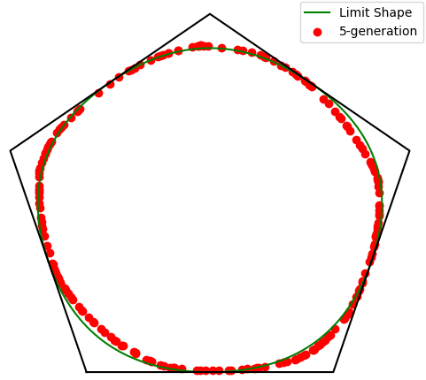
(a) $5$-sampling, $n=200$

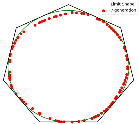
(b) $7$-sampling, $n=100$

Figure 14: Two examples of $\kappa$-sampling. The set of points in red is the set of vertices of a convex $z[n]$-gone, whose boundary we can see to be very close to the limit shape drawn in green.

6.2 Exact and fast algorithm of $\triangle$-sampling

In the triangular case, the algorithm of $\triangle$-sampling avoids the rejection-sampling steps 1 and 2 included in the algorithm of $\kappa$-sampling, which makes the sampling direct and immediately grants a reasonable computation time. Indeed, it happens to be that in the case $\kappa=3$, the joint distribution of $\boldsymbol{\ell}^{(n)}[3],\mathbf{s}^{(n)}[3]$ comes with simplifications (we will show this in B.1), and becomes

$$\mathbb{P}\left(\boldsymbol{\ell}^{(n)}[3]\in\prod_{j=1}^{3}\mathrm{d}\ell_{j},\mathbf{s}^{(n)}[3]=(i,j,k)\right)=\frac{n!\sin(\theta_{\kappa})^{n-3}}{\mathbb{P}_{\triangle}(n)((n-1)!)^{3}}\mathbb{1}_{\ell_{1}+\ell_{2}+\ell_{3}\leq\frac{\sqrt{3}}{2}r_{3}}\\ \times\left(r_{3}-\frac{2}{\sqrt{3}}(\ell_{1}+\ell_{2}+\ell_{3})\right)^{2n-3}{n-1\choose i}{n-1\choose j}{n-1\choose k}\mathbb{1}_{i+j+k=n}\prod_{j=1}^{3}\mathrm{d}\ell_{j}.$$ (130)

Algorithm 2 $\triangle$-sampling

                 Step 1: Sample $s[3]$;

$\bullet$ Draw $(s_{1},s_{2},s_{3})$ as three binomial r.v. $\displaystyle\mathcal{B}(n-1,\frac{1}{2})$ conditioned by $s_{1}+s_{2}+s_{3}=n$.

$\bullet$ $N[3]\leftarrow\left(s_{1}+s_{2}-1,s_{2}+s_{3}-1,s_{3}+s_{1}-1\right)$;

                 Step 2: Sample $\ell[3]$;

$\bullet$ Draw $2n$ uniform $(u_{1},\ldots,u_{2n})$ in the segment $[0,r_{3}]$;

$\bullet$ Sort them into $(u_{(1)},\ldots,u_{(2n)})$;

$\bullet$ $\ell[3]\leftarrow(u_{(1)},u_{(2)}-u_{(1)},u_{(3)}-u_{(2)});\text{\it\# only the first 3 $u_{(i)}$ are used}$

$\bullet$ Compute $c=r_{3}-(\ell_{1}+\ell_{2}+\ell_{3})$;

                 Step 3: Compute ${z}[n]$;

for $1\leq j\leq 3$ do{

         Pick uniformly $N_{j}$ points among the $u_{(j)},j\in\{4,\ldots,2n\}$ to form a partition of $[0,c]$: $(u^{(j)}_{(1)},\ldots,u^{(j)}_{{(N_{j})}});$

         Build $\Delta u^{(j)}[N_{j}+1]=(u^{(j)}_{(1)},u^{(j)}_{(2)}-u^{(j)}_{(1)}\ldots,u^{(j)}_{{(N_{j})}}-u^{(j)}_{{(N_{j}-1)}},c-u^{(j)}_{{(N_{j})}})$;}

end for

for $1\leq j\leq 3$ do{

         Build the vectors $v_{k}^{(j)}=A_{j}(\frac{\pi}{3})^{-1}\begin{pmatrix}\Delta u^{{(j-1)}}_{s_{j-1}+k}\\ \Delta u^{{(j)}}_{k}\end{pmatrix}$ for $1\leq k\leq s_{j}$;

         Sort them into $(v_{(1)}^{(j)},\ldots,v_{(s_{j})}^{(j)})$ by increasing slope;}

end for

$\bullet$ Gather vectors into $v[n]=(v_{(1)}^{(1)},\ldots,v_{(s_{1})}^{(1)},\ldots,v_{(1)}^{(3)},\ldots,v_{(s_{3})}^{(3)})$;

$\bullet$ Build the equilateral triangle $T$ of side length $c$ at distance $\ell[3]$ from the sides of $\mathfrak{C}_{3}$;

$\bullet$ The vectors $(v_{(1)},\ldots,v_{(n)})$, sorted by increasing slope, form the boundary of a convex polygon circumscribed in $T$. The set of its vertices is a $n$-tuple ${z}[n]$ in convex position.

To draw $(s_{1},s_{2},s_{3})$ according to three binomial distributions $\displaystyle\mathcal{B}(n-1,\frac{1}{2})$ and conditioned by $s_{1}+s_{2}+s_{3}=n$, we may:
$\bullet$ Draw $3n-3$ Bernoulli($\frac{1}{3}$) r.v. $\mathbf{x}[3n-3]$;
$\bullet$ Set $(s_{1},s_{2},s_{3})=\left(\sum_{i=1}^{n-1}\mathbf{x}_{i},\sum_{i=n}^{2n-2}\mathbf{x}_{i},\sum_{i=2n-1}^{3n-3}\mathbf{x}_{i}\right)$;
$\bullet$ Correct $\mathbf{x}[3n-3]$ to have $\sum_{i=1}^{3n-3}\mathbf{x}_{i}=n$. The binomial correction works the following way : if $\sum_{i=1}^{3n-3}\mathbf{x}_{i}=n$ then we have the right distribution. Otherwise, if $\sum_{i=1}^{3n-3}\mathbf{x}_{i}<n$, pick uniformly some $j\in\{i;\mathbf{x}_{i}=0\}$ and put $\mathbf{x}_{j}=1$ until $\sum_{i=1}^{3n-3}\mathbf{x}_{i}=n$. If $\sum_{i=1}^{3n-3}\mathbf{x}_{i}>n$ though, pick uniformly some $j\in\{i;\mathbf{x}_{i}=1\}$ and put $\mathbf{x}_{j}=0$ until $\sum_{i=1}^{3n-3}\mathbf{x}_{i}=n$.

At the end we get that

$$\mathbb{P}_{\operatorname{Alg}}\left(\mathbf{s}^{(n)}[3]=(i,j,k)\right) \leavevmode\nobreak\ \propto\leavevmode\nobreak\ {n-1\choose i}\left(\frac{1}{2}\right)^{i}\left(\frac{1}{2}\right)^{n-1-i}{n-1\choose j}\left(\frac{1}{2}\right)^{n-1}{n-1\choose k}\left(\frac{1}{2}\right)^{n-1}\mathbb{1}_{i+j+k=n}$$

$$\leavevmode\nobreak\ \propto\leavevmode\nobreak\ {n-1\choose i}{n-1\choose j}{n-1\choose k}\mathbb{1}_{i+j+k=n}.$$ (131)

The analysis of the sampling of $\boldsymbol{\ell}_{n}[3]$ is the same as in the general $\kappa$-sampling. In the end, the algorithm of $\triangle$-generation admits a global complexity of $\mathcal{O}\left(n\log(n)\right)$ (in expectation).

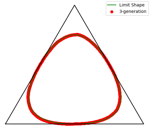
Figure 15: A $\triangle$-sampling, some ${z}[n]$-gone for $n=1000$, close to the limit shape

6.3 Exact and fast algorithm of ${\Box}$-sampling

In the square case, a fast ${\Box}$-sampling can be proposed, which is slightly different from the ${\triangle}$-sampling and from the ${\kappa}$-sampling.

Indeed, in this case, no affine mapping intervenes in the proof since all corners are already right triangles. We may thus consider the law of the positive $x$-components $\mathbf{i}_{n}=\mathbf{s}_{4}^{(n)}+\mathbf{s}_{1}^{(n)}$ and $y$-components $\mathbf{j}_{n}=\mathbf{s}_{1}^{(n)}+\mathbf{s}_{2}^{(n)}$ of the vectors forming the boundary of a ${z}[n]$-gone. A quick calculus allows to compute

$$\mathbb{P}\left(\boldsymbol{\ell}_{n}[4]\in\prod_{j=1}^{4}\mathrm{d}\ell_{j},\mathbf{i}_{n}=i,\mathbf{j}_{n}=j\right)=\frac{(n!)^{2}}{\mathbb{P}_{\Box}(n)((n-1)!)^{4}}\mathbb{1}_{\ell_{1}+\ell_{3}\leq 1}\mathbb{1}_{\ell_{2}+\ell_{4}\leq 1}\left(1-(\ell_{1}+\ell_{3})\right)^{n-2}\\ \times\left(1-(\ell_{2}+\ell_{4})\right)^{n-2}{n-1\choose i}{n-1\choose i-1}{n-1\choose j}{n-1\choose j-1}\prod_{j=1}^{4}\mathrm{d}\ell_{j}.$$ (132)

In particular, this proves that $\mathbf{i}_{n},\mathbf{j}_{n}$ are independent, and their law is explicit. It is easier to draw according to this distribution rather than considering $\mathbf{s}^{(n)}[4].$ This approach is, once more, inspired by Valtr’s paper [23].

Algorithm 3 $\Box$-sampling

                 Step 1: Sampling of $\mathbf{i},\mathbf{j}$;

$\bullet$ For both $\mathbf{i}$ and $\mathbf{j}$, draw two binomials r.v. $\mathcal{B}(n-1,\frac{1}{2})$ until their sum reaches $n$ and set $\mathbf{i}$ (or $\mathbf{j}$) as the result of the first.

                 Step 2: Sampling of $\ell[4]$;

$\bullet$ Draw $n$ i.i.d. uniform r.v. $(u_{1},\ldots,u_{n})$ in the segment $[0,1]$ and sort them into $(u_{(1)},\ldots,u_{(n)})$;

$\bullet$ $(\ell_{1},\ell_{3})\leftarrow(u_{(1)},u_{(2)}-u_{(1)});\text{ \it\# use the 2 smallest}$

$\bullet$ Draw $n$ i.i.d. uniform r.v. $(\hat{u}_{1},\ldots,\hat{u}_{n})$ in the segment $[0,1]$ and sort them into $(\hat{u}_{(1)},\ldots,\hat{u}_{(n)})$;

$\bullet$ $(\ell_{2},\ell_{4})\leftarrow(\hat{u}_{(1)},\hat{u}_{(2)}-\hat{u}_{(1)});$

$\bullet$ Compute $c_{1}=1-(\ell_{1}+\ell_{3})$ and $c_{2}=1-(\ell_{2}+\ell_{4})$;

                 Step 3: Compute ${z}[n]$;

$\bullet$ Pick uniformly $\mathbf{i}$ points $(x_{1}<\ldots<x_{\mathbf{i}})$ among the $u_{(k)},k\in\{3,\ldots,n\}$ and form $h^{+}[\mathbf{i}+1]=(x_{1},x_{2}-x_{1},\ldots,c_{1}-x_{\mathbf{i}})$ (positive increments). The $n-2-\mathbf{i}$ points $(\tilde{x}_{1}<\ldots<\tilde{x}_{n-2-\mathbf{i}})$ remaining in $u_{(k)},k\in\{3,\ldots,n\}$ are used to form $h^{-}[n-1-\mathbf{i}]=(-\tilde{x}_{1},-\tilde{x}_{2}+\tilde{x}_{1},\ldots,-c_{1}+\tilde{x}_{n-2-\mathbf{i}})$ (negative increments);

$\bullet$ Pick uniformly $\mathbf{j}$ points $(y_{1}<\ldots<y_{\mathbf{j}})$ among the $\hat{u}_{(k)},k\in\{3,\ldots,n\}$ and form $v^{+}[\mathbf{j}+1]=(y_{1},y_{2}-y_{1},\ldots,c_{1}-y_{\mathbf{j}})$ (positive increments). The $n-2-\mathbf{j}$ points $(\tilde{y}_{1}<\ldots<\tilde{y}_{n-2-\mathbf{j}})$ remaining in $\hat{u}_{(k)},k\in\{3,\ldots,n\}$ are used to form $v^{-}[n-1-\mathbf{j}]=(-\tilde{y}_{1},-\tilde{y}_{2}+\tilde{y}_{1},\ldots,-c_{1}+\tilde{y}_{n-2-\mathbf{j}})$ (negative increments);

$\bullet$ $h[n]={\sf Merge}(h^{+},h^{-})$ and $v[n]={\sf Merge}(v^{+},v^{-})$;

$\bullet$ Pick uniformly in $\mathcal{S}_{n}$ a permutation $\sigma$ and build for $1\leq i\leq n$ the vector $w_{i}=(h_{i},v_{\sigma(i)})$;

$\bullet$ Sort them into $(w_{(1)},\ldots,w_{(n)})$ by increasing slope;

$\bullet$ Build the rectangle $R$ of side length $c_{1}$ (horizontally) and $c_{2}$ (vertically) at distance $\ell[4]$ from the sides of $\mathfrak{C}_{4}$;

$\bullet$ The vectors $(w_{(1)},\ldots,w_{(n)})$, sorted by increasing slope, form the boundary of a convex polygon inscribed in $R$. The set of its vertices is a $n$-tuple ${z}[n]$ in convex position.

The law of a r.v. $\mathbf{k}$ described in the first step satsifies:

$$\mathbb{P}(\mathbf{k}=k)\leavevmode\nobreak\ \propto\leavevmode\nobreak\ {n-1\choose k}{n-1\choose d}\mathbb{1}_{k+d=n}={n-1\choose k}{n-1\choose k-1}.$$

The probability that two binomial samples are equal is typically $\frac{1}{\sqrt{n}}$. A binomial sampling requires $\mathcal{O}\left(n\right)$ operations, and since this step is the costliest in the $\Box$-generation, the whole algorithm reaches a global complexity of $\mathcal{O}(n^{3/2})$.

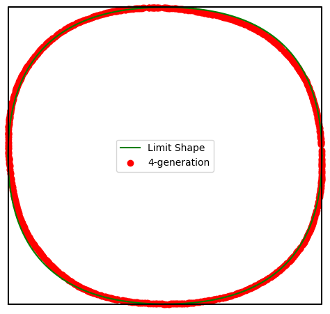
Figure 16: A $\Box$-sampling, some ${z}[n]$-gone for $n=1000$, close to the limit shape

Appendix A Proof of Lemma 2.8

We decompose $\mathbb{P}_{\kappa}(n)$ according to the number of sides of the $\mathsf{ECP}$ we are considering.

Let $\mathbf{z}[n]$ under $\mathbb{U}^{(n)}_{\kappa}$, and write

$$\mathbb{P}_{\kappa}(n) =n!\sum_{\begin{subarray}{c}\mathcal{J}\subset\{1,\ldots,\kappa\}\\ |\mathcal{J}|\geq 3\end{subarray}}\mathbb{P}\left(\mathbf{z}[n]\in\overset{\curvearrowleft}{\mathcal{C}_{\kappa}}(n)\cap\operatorname{NZS}(\mathbf{z}[n])=\mathcal{J}\right).$$

We now borrow to Bárány ([2],[3]) some considerations:

Definition A.1.

Given $S$ a convex compact set (nonflat), let $x_{1},\ldots,x_{m},x_{m+1}=x_{1}$ a subdivision of the boundary $\partial S$ and let $d_{i}$ be the line supporting $S$ at $x_{i}$ for all $i\in\{1,\ldots,m\}$. Write $y_{i}$ for the intersection of $d_{i}$ and $d_{i+1}$ (if $d_{i}=d_{i+1}$ then $y_{i}$ can be any point between $x_{i}$ and $x_{i+1}$). Let $T_{i}$ denote the triangle with vertices $x_{i},y_{i},y_{i+1}$ and also its area. We define the affine perimeter of the convex set $S$ as

$$\operatorname{AP}(S)=2\lim\sum_{i=1}^{m}\sqrt[3]{T_{i}}$$

where the limit is taken over all sequences of subdivisions $x[m]$ with $\max_{1,\ldots,m}|x_{i}-x_{i+1}|\to 0.$

Theorem A.2 (Limit Shape Theorem, Bárány [2]).

Let $K$ be a compact convex domain of $\mathbb{R}^{2}$ with nonempty interior.

1. There exists a convex domain ${\sf Dom}(K)\subset K$ such that $\operatorname{AP}({\sf Dom}(K))>\operatorname{AP}(S)$ for all convex set $S\subset K$ different from ${\sf Dom}(K).$

2. Let $n\geq 3$, and take $\mathbf{z}[n]$ under $\mathbb{Q}_{K}^{(n)}$. Then for all $\varepsilon>0$,

   $$\lim_{n\to+\infty}\mathbb{P}\left(d_{H}({\sf CH}(\mathbf{z}[n]),{\sf Dom}(K))<\varepsilon\right)=1.$$

Definition A.3.

Define $\operatorname{AP}^{*}(K)=\max\{\operatorname{AP}(S),S\text{ convex sets included in }K\}.$

In the case of the regular $\kappa$-gons, the following result comes as a corollary of the properties of the affine perimeter:

Lemma A.4.

Let $x_{1},\ldots,x_{\kappa}$ be the midpoints of the consecutives sides of $\mathfrak{C}_{\kappa}$, and $y_{1},\ldots,y_{\kappa}$ the vertices of $\mathfrak{C}_{\kappa}$, so that $x_{i}$ is the middle of the segment $[y_{i},y_{i+1}]$ (modulo $\kappa$). Let $\mathcal{C}_{i}$ be the unique parabola tangent to $x_{i}y_{i+1}$ at $x_{i}$ and tangent to $y_{i+1}x_{i+1}$ at $x_{i+1}.$ The convex domain ${\sf Dom}(\mathfrak{C}_{\kappa})$ is the subset of $\mathfrak{C}_{\kappa}$ whose boundary is formed by the parabolas $(\mathcal{C}_{i})_{1\leq i\leq\kappa}$. The set ${\sf Dom}(\mathfrak{C}_{\kappa})$ is thus tangent to $\mathfrak{C}_{\kappa}$ in the $\kappa$ points $x_{1},\ldots,x_{\kappa}$.

       

Figure 17: For each case, $\kappa=3$, 4 and 6, the inner curve drawn in red is the boundary of the domain ${\sf Dom}(\mathfrak{C}_{\kappa})$. By the limit shape theorem, it also represents the boundary of a $\mathbf{z}[n]$-gone where $\mathbf{z}[n]$ is taken under $\overset{\curvearrowleft}{\mathbb{Q}}^{(n)}_{\kappa}$, when $n\to+\infty$.

Proof.

A.2 indicates that ${\sf Dom}(\mathfrak{C}_{\kappa})$ is the convex domain contained in $\mathfrak{C}_{\kappa}$ which maximizes the affine perimeter. The general properties of the affine perimeter give the fact that such a subdivision is only reached by the parabolas described in the lemma (see [2] for example). ∎

Lemma A.5.

For all $\kappa\geq 3$, the supremum of affine perimeters $\operatorname{AP}^{*}(\mathfrak{C}_{\kappa})$ is

$$\operatorname{AP}^{*}(\mathfrak{C}_{\kappa})=\operatorname{AP}({\sf Dom}(\mathfrak{C}_{\kappa}))=\kappa\left(r_{\kappa}^{2}\sin(\theta_{\kappa})\right)^{\frac{1}{3}}.$$

Proof.

The subdivision of points $x[m]$ in A.1 maximizing the affine perimeter of a convex domain contained in $\mathfrak{C}_{\kappa}$ is the subdivision composed of the midpoints of the sides of $\mathfrak{C}_{\kappa}$ (meaning $m=\kappa$). Therefore, the hatched areas in Figure 2 are those of the triangles $T_{i}$ introduced in A.1 : This means that for all $i\in\{1,\ldots,\kappa\}$,

$$\sqrt[3]{T_{i}}=\bigg{(}\frac{r_{\kappa}}{2}\sin(\theta_{\kappa}/2)\frac{r_{\kappa}}{2}\cos(\theta_{\kappa}/2)\bigg{)}^{1/3}=\frac{1}{2}\left(r_{\kappa}^{2}\sin(\theta_{\kappa})\right)^{1/3}.$$

Now back to definition A.1,

$$\operatorname{AP}^{*}(\mathfrak{C}_{\kappa})=2\sum_{i=1}^{\kappa}\sqrt[3]{T_{i}}=\kappa\left(r_{\kappa}^{2}\sin(\theta_{\kappa})\right)^{1/3}.$$

∎

Proof of 2.8 :.

For a $n$-tuple $\mathbf{z}[n]$ under $\mathbb{U}^{(n)}_{\kappa}$, Bárány’s A.2 states that for all $\varepsilon>0$,

$$\mathbb{P}\big{(}d_{H}({{\sf CH}}(\mathbf{z}[n]),{\sf Dom}(\mathfrak{C}_{\kappa}))>\varepsilon\leavevmode\nobreak\ |\leavevmode\nobreak\ \mathbf{z}[n]\in\overset{\curvearrowleft}{\mathcal{C}_{\kappa}}(n)\big{)}\underset{n\to+\infty}{\longrightarrow}0,$$

which implies immediately that

$$\mathbb{P}\big{(}\operatorname{NZS}(\mathbf{z}[n])=\{1,\ldots,\kappa\}\leavevmode\nobreak\ |\leavevmode\nobreak\ \mathbf{z}[n]\in\overset{\curvearrowleft}{\mathcal{C}_{\kappa}}(n)\big{)}=\frac{\widetilde{\mathbb{P}}_{\kappa}(n)}{\mathbb{P}_{\kappa}(n)}\underset{n\to+\infty}{\longrightarrow}1.$$

∎

Appendix B Valtr’s results

The surprising simplicity of Valtr’s formulas in the cases of the parallelogram and the triangle can be seen as a consequence of the fact that the sets $\mathcal{L}_{4}$ and $\mathcal{L}_{3}$ are easily computable. Let us recover these results with 3.6.

B.1 The triangle

Theorem B.1 (Valtr [24]).

For all $n\geq 3$, we have

$$\mathbb{P}_{\triangle}(n)=\frac{2^{n}(3n-3)!}{(2n)!((n-1)!)^{3}}.$$

We propose a new proof of Valtr’s result:

Proof.

In the case $\kappa=3$, the side length of $\mathfrak{C}_{3}$ is $r_{3}=2/3^{1/4}$. Pick $c_{1},c_{2},c_{3},\ell_{1},\ell_{2},\ell_{3}$ verifying equations $(\mathcal{C}_{j})_{1\leq j\leq 3}$. Since the only equiangular polygon with three sides is the equilateral triangle, we have $c_{1}=c_{2}=c_{3}=c$. This forces

$$(\mathcal{C}_{1})=(\mathcal{C}_{2})=(\mathcal{C}_{3}):c+\frac{2}{\sqrt{3}}(\ell_{1}+\ell_{2}+\ell_{3})=r_{3}.$$

We thus understand that

$$\mathcal{L}_{3}=\left\{(\ell_{1},\ell_{2},\ell_{3})\in\left[0,\frac{\sqrt{3}}{2}r_{3}\right]^{3}\text{ with }\ell_{1}+\ell_{2}+\ell_{3}\leq\frac{\sqrt{3}}{2}r_{3}\right\}.$$

We also have $\mathbb{N}_{3}(n)=\left\{(i,j,k)\in\{0,\ldots,n-1\}^{3},i+j+k=n\right\},$ so that, we have $\overset{\curvearrowleft}{\mathbb{O}}_{n}^{(3)}=\overset{\curvearrowleft}{\mathbb{Q}}_{n}^{(3)}$ and together with

$$\sum_{s[3]\in\mathbb{N}_{3}(n)}\int_{\mathbb{R}^{3}}f_{n}^{(3)}\left(s[3],\ell[3]\right)\mathrm{d}\ell_{1}\mathrm{d}\ell_{2}\mathrm{d}\ell_{3}=1,$$

we obtain

$$\mathbb{P}_{\triangle}(n)=n!\sin(\frac{\pi}{3})^{n-3}\sum_{s[3]\in\mathbb{N}_{3}(n)}\int_{\ell[3]\in\mathcal{L}_{3}}\prod_{j=1}^{3}\frac{c^{s_{\widebar{j-1}}+s_{j}}}{s_{j}!(s_{\widebar{j-1}}+s_{j})!}\mathrm{d}\ell_{1}\mathrm{d}\ell_{2}\mathrm{d}\ell_{3}.$$

Put $(i,j,k)=s[3]$ and perform the substitution $\ell=\frac{2}{\sqrt{3}}(\ell_{1}+\ell_{2}+\ell_{3})$ to get :

$$\mathbb{P}_{\triangle}(n) =n!\sin(\frac{\pi}{3})^{n-3}\sum_{(i,j,k)\in\mathbb{N}_{3}(n)}\int_{0}^{r_{3}}\frac{1}{2}\ell^{2}\frac{(r_{3}-\ell)^{i+j-1}}{i!(i+j-1)!}\frac{(r_{3}-\ell)^{j+k-1}}{j!(j+k-1)!}\frac{(r_{3}-\ell)^{k+i-1}}{k!(k+i-1)!}\left(\frac{\sqrt{3}}{2}\right)^{3}\mathrm{d}\ell$$

$$=n!\left[\frac{1}{((n-1)!)^{3}}\sum_{i+j+k=n}{n-1\choose i}{n-1\choose j}{n-1\choose k}\right]\left(\frac{\sqrt{3}}{2}\right)^{n}\int_{0}^{r_{3}}\frac{1}{2}\ell^{2}(r_{3}-\ell)^{2n-3}\mathrm{d}\ell$$

$$=\frac{n!}{((n-1)!)^{3}}{3n-3\choose n}\frac{(2n-3)!}{(2n)!}\left(\frac{\sqrt{3}}{2}\right)^{n}r_{3}^{2n}$$

$$=\frac{2^{n}(3n-3)!}{(2n)!((n-1)!)^{3}}.$$

∎

B.2 The square

Theorem B.2 (Valtr [23]).

For all $n\geq 3$, we have

$$\mathbb{P}_{\Box}(n)=\frac{1}{(n!)^{2}}{2n-2\choose n-1}^{2}.$$

Again, we propose a new proof of Valtr’s result:

Proof.

Consider a square (i.e. case $\kappa=4$) of side length $r_{4}=1.$ Pick $c_{1},c_{2},c_{3},c_{4},\ell_{1},\ell_{2},\ell_{3},\ell_{4}$ verifying equations $(\mathcal{C}_{j})_{1\leq j\leq 4}$. Since the only equiangular polygons with four sides are rectangles, we have $c_{1}=c_{3}$ and $c_{2}=c_{4}$ . This implies

$$(\mathcal{C}_{1}=\mathcal{C}_{3}):c_{1}+\ell_{1}+\ell_{3}=1,$$

$$(\mathcal{C}_{2}=\mathcal{C}_{4}):c_{2}+\ell_{2}+\ell_{4}=1.$$

This means in particular that

$$\mathcal{L}_{4}=\big{\{}(\ell_{1},\ell_{2},\ell_{3},\ell_{4})\in[0,1]^{4}\text{ with }\ell_{1}+\ell_{3}\leq 1\text{ and }\ell_{2}+\ell_{4}\leq 1\big{\}}.$$

Just like previously, we have $\overset{\curvearrowleft}{\mathbb{O}}_{n}^{(4)}=\overset{\curvearrowleft}{\mathbb{Q}}_{n}^{(4)}$ so that with

$$\sum_{s[4]\in\mathbb{N}_{4}(n)}\int_{\mathbb{R}^{4}}f_{n}^{(4)}\left(s[4],\ell[4]\right)\mathrm{d}\ell_{1}\mathrm{d}\ell_{2}\mathrm{d}\ell_{3}\mathrm{d}\ell_{4}=1,$$

from what we deduce

$$\mathbb{P}_{\Box}(n)=n!\sum_{s[4]\in\mathbb{N}_{4}(n)}\int_{\ell[4]\in\mathcal{L}_{4}}\prod_{j=1}^{4}\frac{c_{j}^{s_{\widebar{j-1}}+s_{j}}}{s_{j}!(s_{\widebar{j-1}}+s_{j})!}\mathrm{d}\ell_{1}\mathrm{d}\ell_{2}\mathrm{d}\ell_{3}\mathrm{d}\ell_{4},$$

where $\mathbb{N}_{4}(n)=\left\{(s_{1},s_{2},s_{3},s_{4})\in\mathbb{N}^{4}\text{ such that }s_{1}+s_{2}+s_{3}+s_{4}=n\text{ and }s_{j}+s_{\widebar{j+1}}\geq 1\right\}.$ Put $(h,i,j,k)=s[4]$ and perform both substitutions $c_{1}=1-(\ell_{1}+\ell_{3}),c_{2}=1-(\ell_{2}+\ell_{4})$ to get :

$$\mathbb{P}_{\Box}(n) =n!\sum_{(h,i,j,k)\in\mathbb{N}_{4}(n)}\int_{0}^{1}\int_{0}^{1}\frac{(1-c_{1})c_{1}^{h+i-1}}{h!(h+i-1)!}\frac{(1-c_{2})c_{2}^{i+j-1}}{i!(i+j-1)!}\frac{c_{1}^{j+k-1}}{j!(j+k-1)!}\frac{c_{2}^{h+k-1}}{k!(h+k-1)!}\mathrm{d}c_{1}\mathrm{d}c_{2}$$

$$=n!\bigg{(}\int_{0}^{1}(1-c)c^{n-2}\mathrm{d}c\bigg{)}^{2}\sum_{(h,i,j,k)\in\mathbb{N}_{4}(n)}\frac{1}{h!(h+i-1)!}\frac{1}{i!(i+j-1)!}\frac{1}{j!(j+k-1)!}\frac{1}{k!(h+k-1)!}$$ (133)

The integral is a standard beta-integral so that $\displaystyle n!\bigg{(}\int_{0}^{1}(1-c)c^{n-2}\mathrm{d}c\bigg{)}^{2}=n!\left(\frac{(n-2)!}{n!}\right)^{2}.$ It remains to compute the big sum $S$ apart in (B.2):

$$S =\frac{1}{(n-2)!((n-1)!)^{2}}\sum_{(h,i,j,k)\in\mathbb{N}_{4}(n)}{n-1\choose h+i}{n-1\choose j+k}{h+i\choose h}{j+k\choose k}{n-2\choose i+j-1}$$

$$=\frac{1}{(n-2)!((n-1)!)^{2}}\sum_{r=1}^{n-1}{n-1\choose r}{n-1\choose n-r}{2n-2\choose n-1}$$

$$=\frac{1}{n!((n-2)!)^{2}}{2n-2\choose n-1}^{2}.$$

which is Valtr’s formula. ∎

Acknowledgements

I would like to thank Jean-François Marckert for his valuable guidance and advices throughout the long research and writing process of this paper.

I also thank Zoé Varin for her precious help when struggling with Tikz. Some of the figures of this paper were created entirely by her expert hand.

References

- [1] I. Bárány. The limit shape of convex lattice polygons. Discrete Comput. Geom., 13(3-4):279–295, 1995.
- [2] I. Bárány. Affine perimeter and limit shape. Journal für die reine und angewandte Mathematik, 484:71–84, 1997.
- [3] I. Bárány. Sylvester’s question: The probability that n points are in convex position. The Annals of Probability, 27(4):2020–2034, 1999.
- [4] P. Billingsley. Convergence of Probability Measures. Wiley Series in Probability and Statistics. Wiley, 1999.
- [5] W. Blaschke. Über affine geometrie xi: Lösung des “vierpunktproblems” von sylvester aus der theorie der geometrischen wahrscheinlichkeiten. Leipziger Berichte, 69:436–453, 1917.
- [6] O. Bodini, A. Jacquot, P. Duchon, and L. R. Mutafchiev. Asymptotic analysis and random sampling of digitally convex polyominoes. CoRR, abs/1306.2108, 2013.
- [7] M. B. Brown and J. Bromberg. An efficient two-stage procedure for generating random variates from the multinomial distribution. The American Statistician, 38(3):216–219, 1984.
- [8] T. Buffière. Combinatoire et théorèmes probabilistes sur certaines familles de polytopes, 2023.
- [9] J. Bureaux and N. Enriquez. On the number of lattice convex chains. Discrete Analysis, pages 1–15, dec 2016.
- [10] I. Bárány, J. Bureaux, and B. Lund. Convex cones, integral zonotopes, limit shape. Advances in Mathematics, 331:143–169, 2018.
- [11] C. S. Davis. The computer generation of multinomial random variates. Computational statistics & data analysis, 16(2):205–217, 1993.
- [12] H. J. Hilhorst, P. Calka, and G. Schehr. Sylvester’s question and the Random Acceleration Process. Journal of Statistical Mechanics: Theory and Experiment, page P10010, 2008. 29 pages, 4 figures; references added and minor changes.
- [13] M. V. Jambunathan. Some Properties of Beta and Gamma Distributions. The Annals of Mathematical Statistics, 25(2):401 – 405, 1954.
- [14] R. A. Kronmal and A. V. Peterson Jr. On the alias method for generating random variables from a discrete distribution. The American Statistician, 33(4):214–218, 1979.
- [15] J.-F. Marckert. One more approach to the convergence of the empirical process to the brownian bridge. Electronic journal of Statistics, 2:118–126, 2008.
- [16] J.-F. Marckert. The probability that n random points in a disk are in convex position. Brazilian Journal of Probability and Statistics, 31(2):320–337, 2017.
- [17] J.-F. Marckert and S. Rahmani. Around Sylvester’s question in the plane. Mathematika, 67(4):860–884, Aug. 2021.
- [18] V. Petrov. Sums of Independent Random Variables. Ergebnisse der Mathematik Und. Springer-Verlag, 1975.
- [19] R. E. Pfiefer. The historical development of j. j. sylvester’s four point problem. Mathematics Magazine, 62(5):309–317, 1989.
- [20] R. Schneider. Discrete aspects of stochastic geometry. In Handbook of discrete and computational geometry, pages 299–329. Chapman and Hall/CRC, 2017.
- [21] Y. Sinai. Probabilistic approach to the analysis of statistics for convex polygonal lines. Funct Anal Its Appl, 28:108–113, 1994.
- [22] J. J. Sylvester. Problem 1491. The educational Times, 1864.
- [23] P. Valtr. Probability that n random points are in convex position. Discrete and computational geometry, 13(3-4):637–643, 1995.
- [24] P. Valtr. The probability that n random points in a triangle are in convex position. Combinatorica, 16(4):567–573, 1996.
- [25] A. Vershik. The limit shape of convex lattice polygons and related topics. Funct Anal Its Appl, 28:13–20, 1994.
- [26] A. J. Walker. An efficient method for generating discrete random variables with general distributions. ACM Transactions on Mathematical Software (TOMS), 3(3):253–256, 1977.