FargoCPT : A 2D Multi-Physics Code for Simulating the Interaction of Disks with Stars, Planets and Particles

Abstract

Context. Planet-disk interactions play a crucial role in the understanding of planet formation and disk evolution. There are multiple numerical tools available to simulate these interactions, including the often-used FARGO code and its variants. Many of the codes were extended over time to include additional physical processes with a focus on their accurate modeling.

Aims. We introduce FargoCPT, an updated version of FARGO incorporating other previous enhancements to the code, to provide a simulation environment tailored to study interactions between stars, planets, and disks, ensuring accurate representation of planet systems, hydrodynamics, and dust dynamics with a focus on usability.

Methods. The radiation-hydrodynamics part of FargoCPT uses a second-order upwind scheme in 2D polar coordinates supporting multiple equations of state, radiation transport, heating and cooling, and self-gravity. Shocks are considered using artificial viscosity. Integration of the N-body system is achieved by leveraging the REBOUND code. The dust module utilizes massless tracer particles, adapting to drag laws for the Stokes and Epstein regimes. Moreover, FargoCPT provides mechanisms to simulate accretion onto the stars and planets.

Results. The code has been tested in practice by its use in various publications. Additionally, it comes with an automated test suite to test the physics modules.

Conclusions. FargoCPT offers a unique set of simulation capabilities within the current landscape of publicly available planet-disk interaction simulation tools. Its structured interface and underlying technical updates are intended to assist researchers in the ongoing exploration of planet formation.

1 Introduction

Planet migration is a crucial part of our understanding of planet formation. Besides analytical or semi-analytical calculations, one way to study it is by hydrodynamics calculations coupled with gravitational N-body simulations. Specifically, in the context of planet formation, the shape of the hydrodynamic object resembles a thin, flared disk. FARGO (masset_fargo_2000) is a computer program to simulate these protoplanetary disks by numerically solving the hydrodynamics equations on a staggered grid using a second-order upwind scheme. It includes a special algorithm, with the same name, which can relax the time step constraint by making use of the axial symmetry of the disk flow, thereby reducing the computational cost of simulations. The specific form of the hydrodynamics equations solved by the program is stated later in Sect. 2.

Because FARGO is tailored to the study of protoplanetary disks, the code uses a cylindrical grid, reflecting the major symmetry of the system. One main assumption used in the code is that the simulated disks are thin in the sense that their vertical extent is small compared to the radial distance from the central star. This is the justification for approximating the three-dimensional disk with a two-dimensional representation. Using this approximation significantly reduces the required time for simulations of protoplanetary disks and enables the long-term study of these systems. In its original form, the code employed the (locally-)isothermal assumption, in which the temperature is assumed to be fixed in time and only dependent on the distance from the central start. This allows solving the energy equation analytically and additionally reduces the computational cost of the simulation.

In the past two decades, studies have shown that additional effects play an important role in the evolution of protoplanetary disks and their interaction with embedded planets (for overviews see kley_planet-disk_2012; baruteau_planet-disk_2014; paardekooper_planet-disk_2023). Relevant physical processes include the heating and cooling of the gas (e.g. baruteauCorotationTorqueRadiatively2008a; kley_migration_2008; paardekooper_disc_2008; lega_migration_2014; masset_coorbital_2017), self-gravity (e.g. pierens_how_2005; baruteauTypePlanetaryMigration2008), and radiation transport (e.g. morohoshi_gravitational_2003; paardekooper_halting_2006). We have added all of these effects to our version of the FARGO code and made them fully controllable from the input file and verified their correctness through extensive testing. We also extended the number of physical quantities that are evaluated during the simulation and written to output files.

While there are multiple options to run planet-disk interaction simulations including the aforementioned effects, the authors recognized a need for a simulation code that is not only able to simulate the relevant physical processes accurately but is also easy to use. This is especially important for students and researchers who are not experts in modifying and compiling C/C++ or FORTRAN codes in a typical Linux environment. These skills can pose a significant hurdle to run simulations.

The primary aim behind publishing this code is to provide a comprehensive simulation tool for planet-disk interactions that remains accessible and useful to both students and more senior researchers. To this end, the testing suite for the physical modules is fully automated with pass-fail tests so it can be run after every future modification of the code to ensure that it is still working as intended.

On the physics side, a significant enhancement is the incorporation of radiation physics. Furthermore, the introduction of a particle module enables in-depth studies on the impact of embedded planet systems on the structure and dust distribution of planet-forming disks, a task that is currently often performed to model disk observations. We also added cooling and mass inflow functions and an updated equation of state specifically tailored to study cataclysmic variable systems. Additionally, the code can simulate the disk centered around any combination of N-body objects. This enables, for instance, simulations of circumbinary disks in the center of mass-frame or simulations of a circumsecondary disk in a binary star system.

Simulation programs for planet-disk interaction can, broadly speaking be organized into two main categories: Lagrangian and Eulerian methods. Lagrangian methods trace the dynamics of the disk by following the motion of a large number of particles. The most common example of this is the Smoothed Particle Hydrodynamics (SPH) method with a prominent example being the PHANTOM code (price_phantom_2018).

The Eulerian methods solve the hydrodynamics equations on a grid, which can either be fixed or dynamic. In this category, again, we can distinguish between two main approaches used in astrophysics: methods that require artificial viscosity and Godunov methods (woodward1984art_vis_and_godunov). Either of these methods can be implemented as a finite-volume or finite-difference method. Godunov methods solve the Riemann problem at the cell interfaces to compute the fluxes through the interfaces which allows for an accurate treatment of shocks and an approximate treatment of smooth flows. Prominent examples include the PLUTO code mignone2007pluto and the Athena++ code (stone_athena_2020).

Schemes based on artificial viscosity can be derived as a finite-difference scheme from Taylor series expansions of the Euler equations (woodward1984art_vis_and_godunov). This technique assumes that the solution is smooth, which is not the case at discontinuities such as shocks. It approximates shocks by smearing out discontinuities into smooth regions of strong gradients via artificial viscosity. The ZEUS code (stone1992zeus1) and the FARGO code (which is based on the ZEUS code) are prominent examples of this approach. While these codes were classified as finite-difference schemes, they employ a staggered grid and implement their advection step by splitting the domain into cells and computing the fluxes through the cell interfaces. The cell as a basic geometrical unit, and the sharing of fluxes among adjacent cells which ensures conservation of the advected quantities to machine-precision by construction, warrant the classification of the advection scheme as finite-volume (anderson_computational_2020). The authors lean towards this classification because it rests on an intrinsic property of the scheme. However, the crucial distinction seems to be the one between Godunov methods and methods that require artificial viscosity and the FARGO code family falls into the latter category.

While formally the Godunov methods are more accurate in handling discontinuities like shocks, the artificial viscosity methods are better at modeling smooth flows and, in practice, are often more robust and easier to use. Both approaches have their advantages and disadvantages and the choice of which method to use depends on the specific problem at hand. For a specific example, see ziampras_buoyancy_2023 who used, both, PLUTO and FARGO3D to investigate buoyancy waves in the coorbital region of small-mass planets.

The original FARGO code was introduced by masset_fargo_2000. Based on this code, other groups developed their version of the FARGO code. Examples include FARGO_THORIN (chrenkoEccentricityExcitationMerging2017), FARGOCA (lega_migration_2014), FARGO2D1D (cridaSimulatingPlanetMigration2007b), and the GFARGO code (regalyPossiblePlanetformingRegions2012a; massetGfargoFargoGpu2015), the predecessor of our code FARGOADSG (baruteauCorotationTorqueRadiatively2008a; baruteauTypePlanetaryMigration2008; baruteauGasDustHydrodynamical2016a), as well as the official successor FARGO3D (benitez-llambayFARGO3DNewGPUoriented2016).

In this work, we present FargoCPT, the FARGO version developed by members of the Computational Physics group at the University of Tübingen since 2012. Publications from this group that used the code include mullerCircumstellarDisksBinary2012; mullerModellingAccretionTransitional2013, picogna_how_2015, rometsch_migration_2020; rometschSurvivalPlanetinducedVortices2021b, and jordanDisksCloseBinary2021.

Furthermore, we present novel approaches for handling challenging aspects of planet-disk interaction simulations. We introduce a new method for handling the indirect term suitable for simulations centered on individual stars in binary systems (Sect. 3.5), a local viscosity stabilizer for use in the context of cataclysmic variables (Sect. LABEL:sec:viscosity_stabilizer) and a correction for dust diffusion treated by stochastic kicks (Sect. LABEL:sec:dust_diffusion).

This document is structured as follows. First, the physical problem at hand is sketched in Sect. 2. Then, the newly introduced physics modules are described in Sect. 3. Software engineering and usability aspects of the code are discussed in Sect. LABEL:sec:software. Finally, the paper is concluded in Sect. LABEL:sec:discussion with a discussion of the code. The Appendix includes a presentation of various test cases included in the automatic test suite.

2 Physical system

The FargoCPT code is a computer program that numerically solves the vertically-integrated radiation-hydrodynamics equations in the one-temperature approximation coupled with an N-body system. They read

$$\frac{\partial\Sigma}{\partial t}+\nabla\cdot(\Sigma\@vec{u}) =0$$ (1)

$$\frac{\partial\Sigma\@vec{u}}{\partial t}+\nabla\cdot(\Sigma\@vec{u}\otimes\@vec{u}) =-\nabla P+\Sigma\@vec{k}+\nabla\tau$$ (2)

$$\frac{\partial e}{\partial t}+\nabla\cdot(e\@vec{u}) =-P\nabla\@vec{u}+\mathcal{S}+\mathcal{RT}$$ (3)

with the surface density $\Sigma=\int_{-\infty}^{\infty}\rho\,\mathrm{d}z$ as the vertically integrated gas volume density $\rho$, the gas velocity $\@vec{u}$, the vertically integrated internal energy density $e=\Sigma\epsilon$ with the specific internal energy $\epsilon$, the vertically integrated pressure $P=\int_{-\infty}^{\infty}p\,\mathrm{d}z$, accelerations $\@vec{k}$ due to external forces (e.g. due to gravity), the viscous stress tensor $\tau$, and heat sinks and sources $\mathcal{S}$ (see Sect. 3.8). The last term represents radiation transport

$$\mathcal{RT}=-\int_{-\infty}^{\infty}\nabla\@vec{F}\mathrm{d}z$$ (4)

with the radiation flux $\@vec{F}$ in three dimensions. In the code, the vertical component of the radiation flux is split off and treated with an effective model, see Sect. 3.8. Please note, that the code handles radiation hydrodynamics using the one-temperature approach which is discussed in more detail in Sect. 3.8.5.

In polar coordinates $(r,\phi)$, to which the code is tailored, the equations read (e.g. massetCoorbitalCorotationTorque2002)

$$\frac{\partial\Sigma}{\partial t}+\frac{1}{r}\frac{\partial\left(ru_{r}\Sigma\right)}{\partial r}+\frac{1}{r}\frac{\partial\left(u_{\phi}\Sigma\right)}{\partial\phi} =0\,,$$ (5)

$$\frac{\partial u_{r}}{\partial t}+u_{r}\frac{\partial u_{r}}{\partial r}+\frac{u_{\phi}}{r}\frac{\partial u_{r}}{\partial\phi}-\frac{u_{\phi}^{2}}{r} =-\frac{1}{\Sigma}\frac{\partial P}{\partial r}+k_{r}+\frac{f_{r}}{\Sigma}\,,$$ (6)

$$\frac{\partial u_{\phi}}{\partial t}+u_{r}\frac{\partial u_{\phi}}{\partial r}+\frac{u_{\phi}}{r}\frac{\partial u_{\phi}}{\partial\phi}+\frac{u_{r}u_{\phi}}{r} =-\frac{1}{\Sigma r}\frac{\partial P}{\partial\phi}+k_{\phi}+\frac{f_{\phi}}{\Sigma}\,,$$ (7)

$$\frac{\partial e}{\partial t}+\frac{1}{r}\frac{\partial\left(ru_{r}e\right)}{\partial r}+\frac{1}{r}\frac{\partial\left(u_{\phi}e\right)}{\partial\phi} =-\frac{P}{r}\frac{\partial\left(ru_{r}\right)}{\partial r}-\frac{P}{r}\frac{\partial u_{\phi}}{\partial\phi}+\mathcal{S}+\mathcal{RT}$$ (8)

where $f_{r}$ and $f_{\phi}$ are the radial and azimuthal forces per unit area due to viscosity (see Eqs. (89) and (90)). For a rotating coordinate system, we follow the conservative formulation of kley1998coriolis and add the respective terms to the two momentum equations.

The l.h.s. of these equations are the transport step and the r.h.s. are the source terms. Following the scheme of the ZEUS code (stone1992zeus1), the transport step is solved by a finite-volume method based on an upwind scheme with a second-order slope limiter (van1977towards) and the code can make use of the FARGO algorithm (masset_fargo_2000) to speed up the simulation. The source terms are updated as described in Sect. 3.1 using first-order Euler steps or implicit updates. The definitions for the heating and cooling term $\mathcal{S}$ and the radiation transport term $\mathcal{RT}$ are given in Sect. 3.8.

The external accelerations $\@vec{k}$ are due to the gravitational forces from the star(s) and planets, correction terms in case of a non-inertial frame, and the self-gravity of the disk

$$\@vec{k}=-\nabla(\Phi_{\mathrm{Nb}}+\Phi_{\mathrm{Ind}})-a_{\mathrm{SG}}\,.$$ (9)

Interaction of the disk with the N-body objects is considered via the gravitational potential, see Eq. (15). Self-gravity of the gas is considered as an acceleration (see Sect. 3.7).

The N-body objects feel the gravitational acceleration $\@vec{a}$ exerted by the gas. This is computed by summation of the smoothed gravitational acceleration over all grid cells. Refer to Sect. 3.6 for formulas and details about the smoothing. Because the simulation can be run in a non-inertial frame of reference, correction terms are applied as detailed in Sect. 3.5.

Finally, FargoCPT features a particle module based on Lagrangian super-particles, where a single particle might represent any number of physical dust particles or solid bodies. The particles feel the gravity from the N-bodies and interact with the gas through a gas-drag law. Additionally, dust diffusion is modeled to consider the effects of gas turbulence. The particle module is described in detail in section LABEL:sec:dust.

The next section describes the various physics modules that were added to the code.

3 Improvements of the physics modules

We built upon the original FARGO code by masset_fargo_2000 and its improved version FARGOADSG . It already included treatment of the energy equation (baruteauCorotationTorqueRadiatively2008a), self-gravity (baruteauTypePlanetaryMigration2008), and a Lagrangian particle module (baruteauGasDustHydrodynamical2016a). We advanced these modules, added new physics modules, and added features to improve the usability of the code. For a detailed description of the FARGOADSG code, and with it of the underlying hydrodynamics part of the code presented here, we recommend Chapter 3 of baruteauPredictiveScenariosPlanetary2008a.

This section starts with outlining the order of operations in the operator splitting approach and then describes the various new features and changes.

3.1 Order of operations and interaction of subsystems

This section details the order in which the physical processes are considered during one iteration in the code and how they interact.

For the update step, we used the sequential operator splitting (also known as Lie-Trotter splitting) where possible, meaning that we always use the most up-to-date quantities from the previous operators when applying the current operator. This is the simplest and oldest splitting scheme and has better accuracy than applying all operators using the quantities at the beginning of the step. This scheme is called additive splitting (e.g. geiser2017new). Each time step starts with accretion onto the planets. Conceptually, this is the same as performing planet accretion at the end of the time step, except for the first and last iteration of the simulation.

Then, we compute the gravitational forces between the N-body objects and the gas, between the N-body objects and the dust particles, and the self-gravity of the disk. At this stage, the indirect term, i.e. the corrections for the non-inertial frame, is computed and added to the gravitational interaction. These are then applied to the subsystems by updating the velocity of the N-body objects, by updating the acceleration of the dust particles, and by updating the potential of the gas. Experience shows, that for the interaction between N-body and gas the positions of the N-body objects have to be at the same time as the gas. From this point on, the N-body system and the particle system evolve independently in time until the end of the time step.

The gas velocities are first updated by the self-gravity acceleration and then by the N-body gravity potential, the pressure gradient, and, in the case of the radial update, also the centrifugal acceleration. At this step, we update the internal energy of the gas with compression heating. It is important to perform the energy update at this step before the viscosity is applied to avoid instabilities. Then, we sequentially update velocities and the internal energy further by artificial viscosity, then viscosity (both of which depend on the gas velocities), and then apply heating and cooling terms as well as radiation transport. The heating and cooling steps are applied simultaneously for numerical stability. Finally, the internal energy is updated by radiation transport.

Once all the forces and source terms are applied, we conduct the transport step. Boundary conditions and the wave-damping zone are applied at the appropriate sub-steps throughout the hydrodynamics step.

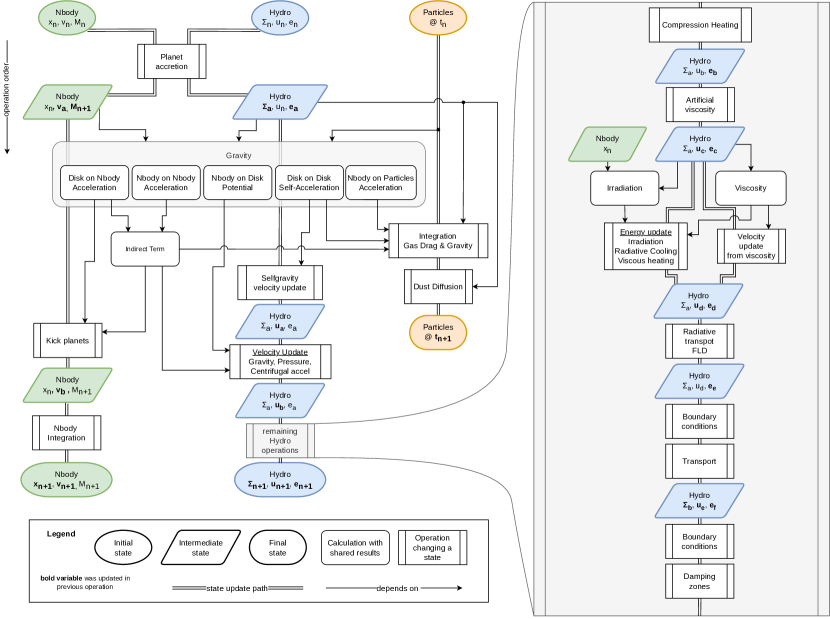
Figure 1: Order of operations in the operator splitting scheme showing the evolution of the N-body, hydro, and particle subsystems throughout one iteration step. Single-line arrows mean that the originating object is used in the calculation of the destination. Double lines indicated the evolution of one of the subsystems from the initial state (ellipse) over intermediate states (parallelogram) to the final state (round shape). Each rectangle with rounded corners is a computation of an intermediate quantity using the state of the subsystem to which it is connected. The rectangles with bars on the sides indicate an operation that changes the state of a system. The variables that were changed by an operation are indicated in boldface in the intermediate states.

A detailed diagram of the order of the operations during each time step and the interactions between the subsystems are shown in Fig. 1. The diagram illustrates how each of the subsystems is advanced in time and between which sub-steps information is exchanged between the subsystems. The next paragraphs guide through the diagram starting from the top, explaining the meaning of the differently shaped patches, arrows and lines.

Each of the three subsystems is colored differently: the N-body system is shown in green, the hydrodynamics in blue and the dust particles in orange. A colored patch represents the state of a subsystem. Elliptical patches indicate the initial state at the beginning of a time step, parallelograms indicate intermediate states and colored rectangles with rounded corners indicate the final state at the end of the time step. Each state is labeled with variable names. The respective subscript indicates the the sub-step during the operator splitting. For example, the energy is updated from $e_{n}$, first to $e_{a}$, then to $e_{b}$ and after additional steps finally to $e_{n+1}$. These variables will be used in Sect. 3.8 to refer to the sub-steps. A variable printed in bold text indicates that the variable was changed by the last operation.

A white rectangle with rounded corners indicates an intermediate calculation, the result of which is used in multiple operations. For example, the calculation of the indirect term is used in all three subsystems. Finally, the rectangles with bars on the sides indicate an operation that changes the state of a system.

Double lines trace the change of a subsystem throughout the time step. Lines with arrows attached at the end emerge from a state patch or an intermediate calculation and end in an operation or intermediate calculation patch.

The large rectangle with bars shaded in grey at the right side of the diagram illustrates the sub-steps involved in the hydrodynamics part of the simulation. Except for the irradiation operation which requires the position of the N-bodies, this part of the simulation is independent of the N-body system.

The shaded rectangle with rounded corners in the upper third of the diagram illustrates the various gravitational interactions between the subsystems. The information indicated by arrows that end at the borders of this patch can be applied in any of the contained intermediate calculations.

The operations are ordered from the top to bottom in the order they are applied during the time step. This means, that an operation or a state is generally only influenced by states above it or at the same level. Please follow the arrows to get a sense of the order of operations.

3.2 N-body module

The original FARGO code includes a Runge-Kutta fifth-order N-body integrator, which was used with the same time step as the hydro simulations. This could lead to some situations in which the time step was too large for the N-body simulation, for instance, during close encounters in simulations of multiple migrating planets. Instead of implementing our N-body code with adaptive time-stepping, we incorporated the well-established and well-tested Rebound code (rein_rebound_2012) with its 15th order IAS15 integrator (rein_ias15_2015) into FargoCPT . Rebound is called during every integration step of the hydro system to advance the N-body system for the length of the CFL time step. During this time, multiple N-body steps might be performed as needed. The interaction with the gas is incorporated by adding $\Delta t\,\@vec{a}$ to the velocities of the bodies before the N-body integration.

We changed the central object from an implicit object, which was assumed to be of mass 1 in code units placed at the origin, to a moving point mass. It is now treated exactly like any other N-body object, notably including gravitational smoothing, which was not applied to the star before This solves an inconsistency between the interaction of disk and planets, and disk and star. This is necessary as the smoothing simulates the effect of the disk being stratified in the vertical direction and makes the potential behave more like it would in 3D (mullerTreatingGravityThindisk2012).

Changing the star from being an implicit object to an explicit one, we changed all the relevant equations, which now include the mass of the central object and the distance to it.

3.3 Gravitational interactions

The dominating physical interaction between planets and a disk is gravity. In principle, any object that has mass causes a gravitational acceleration on any other object.

In our simulation, N-body objects are considered to have a mass and particles are considered to be massless. The gas disk can be configured in one of three states. The gas disk can

1. be massless and not accelerate the N-bodies.

2. have mass, accelerate the N-bodies, the particles and itself (self-gravity included).

3. have mass, accelerate the N-bodies, but not itself or the particles (self-gravity ignored).

The first two cases are consistent whereas the third case is inconsistent. However, it is a commonly used approximation. The reason for this is that the computation of the (self-)gravity of the gas disk is computationally expensive.

In the third case, when the forces on the N-bodies due to the gas are computed using the full surface density, the N-bodies feel the full mass of the disk interior to their orbit while gas on the same orbit does not feel this mass. Consequently, their respective equilibrium state angular velocities differ which causes a nonphysical shift in resonance locations and thus in the torque and migration rate experienced by the planets (baruteauTypePlanetaryMigration2008). This mismatch can be alleviated by simply subtracting the azimuthal average of the surface density in the calculation of the force. This is done in the code in the case that self-gravity is disabled.

Our code does not support a configuration in which only one of the N-bodies feels the disk, such as a situation in which the planet feels the disk but the star does not. This is done intentionally to avoid nonphysical systems. Likewise, the indirect term caused by the disk is always included if the disk has mass (cases 2 and 3).

Whether the disk is considered to have mass is configured by the DiskFeedback option. If this is set to yes, the disk is considered to have mass and vice-versa. The three cases and the value of the code parameters are summarized in Table 1.

Table 1: Possible cases for the disk gravity.

Case	N-body	Particles	Disk	DiskFeedback	SelfGravity
massless	no	no	no	no	no
massive w/o sg	yes	no	no	yes	no
massive	yes	yes	yes	yes	yes

3.4 Coordinate center

Because the star is treated like any other N-body object and can move, we need to define the coordinate center of the hydro domain. In principle, we can choose an arbitrary reference point. However, because the N-body system dominates the gravity, we choose the center of mass of any combination of N-bodies as the coordinate center.

With the N-body objects located at $\@vec{r}_{i}$, with $i=1,2,\dots,N_{p}$, the coordinate center $\@vec{R}$ can now be set as

$$\@vec{R}=\frac{1}{\sum_{i=1}^{N_{c}}M_{i}}\sum_{i=1}^{N_{c}}M_{i}\,\@vec{r_{i}}\,,$$ (10)

where $N_{c}$ is the number of point masses whose center of mass is chosen to be the coordinate center. For example, $N_{c}=N_{p}$ selects the full N-body system as a reference, $N_{c}=1$ selects the primary as a center, and $N_{c}=2$ selects a stellar binary or the center of mass of a star-planet system.

The center of mass of the full N-body system is likely the most desirable of such choices because it can be an inertial frame that does not require considering fictitious forces. This eliminates the need for an extra acceleration term to correct for the non-inertial frame, the so-called indirect term, which can be the source of numerical instabilities. At least it eliminates the need for the indirect term resulting from the N-body system which generally dominates the indirect term, though contributions from the disk gravity might still need to be considered.

An application is the simulation of circumbinary disks, in which the natural coordinate center is the center of mass of the binary stars.

3.5 Shift-based indirect term

The correction forces needed because of a non-inertial frame are typically called the indirect term in the context of planet-disk interaction simulations. Based on the definition of the coordinate center in Eq. (10), the corresponding acceleration can formally be written as

$$\@vec{a}_{\text{Ind}}=-\frac{\text{d}^{2}}{\text{d}t^{2}}\@vec{R}=-\frac{1}{M_{c}}\sum_{i=1}^{N_{c}}M_{i}\,\@vec{a_{i}}\,,$$ (11)

where we used $\@vec{a}_{i}=\ddot{\@vec{r}_{i}}$, defined $M_{c}=\sum_{i=1}^{N_{c}}M_{i}$, and assumed that the derivatives of the masses are negligible. The individual $\@vec{a}_{i}$ should include all accelerations from forces acting on a specific N-body $i$, including gravity from all sources, other N-bodies or the disk.

Usually, this correction term is evaluated at the start of a time step, yielding a vector $\@vec{a}_{\text{Ind}}^{t}$. As outlined in Sect. 2, this is then added to the velocities of the N-bodies as a sort of Euler step $\@vec{v}_{i}^{t\prime}=\@vec{v}_{i}+\Delta t\@vec{a}_{\text{Ind}}^{t}$ before integration of the N-body system. For the disk, the indirect term is applied through the potential. This update is first-order in time. As long as the magnitude of the indirect term is small compared to direct gravity, this choice appears to be good enough.

Using an Euler step as above is not sufficient in simulations in which the indirect term becomes stronger than the direct gravity. This can be the case in simulations of circumbinary disks centered on one of the stars which are useful for the study of circumstellar disks in binary star systems. In such simulations, the disk can become unstable with the Euler method.

As a solution, we compute the indirect term as the average acceleration felt by the coordinate center during the whole time step. The average acceleration is computed from the actual shift needed to keep the coordinate center put. Therefore we call this method the shift-based indirect term. In our code, this is achieved by making a copy of the N-body system after the N-body velocities have been updated by disk gravity, integrating the copy in time and computing the net acceleration from the velocities as

$$\@vec{a}_{\mathrm{Ind}}=-\frac{\@vec{v}_{c}^{t+\Delta t}-\@vec{v}_{c}^{t}}{\Delta t}.$$ (12)

where $\@vec{v}_{c}=\frac{\text{d}}{\text{d}t}\@vec{R}$ is the velocity of the coordinate center. We then discard the N-body system copy, apply this indirect term to the N-body, hydro and particle systems and integrate them. This way, the acceleration of the center and the indirect term cancel out and the system stays put much better compared to the old method. Note, that the computation of the acceleration is handled this way because the IAS15 is a predictor-corrector scheme that does not produce an effective acceleration that would be accessible from the outside. Using the acceleration from an explicit Runge-Kutta scheme would produce the same results.

We tested, both, the old and the shift-based indirect term implementations and could not find any discernable difference in the dynamics of systems with embedded planets as massive as 10 Jupiter masses around a solar mass star. However, the shift-based indirect term enables simulations of circumbinary disks centered on one of the stars which was previously not possible. Even resolved simulations of circumsecondary disks (centered on the secondary star) when the latter is less massive than the primary star are possible. For the impact of this new scheme on the simulation of circumbinary disks, see Jordan et al. (2024, in prep).

3.6 Gravity and Smoothing

For modeling gravity, we use the common scale-height-dependent smoothing approach. This approach accounts for the fact that a gas cell in 2D, that represents a vertically extended disk, feels a weaker gravitational pull from an N-body object compared to the same cell for a truly razor thin 2D disk (mullerTreatingGravityThindisk2012). The potential due to a point mass $k$ with mass $M_{k}$ at a distance $d_{ik}$ from the center of a cell $i$ is then given by

$$\Phi_{k}=-\frac{\mathrm{G}M_{k}}{\sqrt{d_{ik}^{2}+\epsilon_{i}^{2}}}$$ (13)

where $\mathrm{G}$ is the gravitational constant, $d_{ij}$ is the distance between the point mass and the cell, and $\epsilon_{i}=\alpha_{\text{sm}}H_{i}$ is the smoothing length with the smoothing parameter $\alpha_{\text{sm}}$ and the cell scale height $H_{i}$. According to mullerTreatingGravityThindisk2012, $\alpha_{\text{sm}}$ should be between 0.6 – 0.7 to accurately describe gravitational forces and torques, which is why we apply it to all N-bodies, even the central star. massetCoorbitalCorotationTorque2002 found that a factor of 0.76 most closely reproduces type I migration rates of 3D simulations. Please note that $\epsilon_{i}$ has to be evaluated with the scale height at the location of the cell, not the location of the N-body object (mullerTreatingGravityThindisk2012).

When the gravity of planets inside the disk is also considered for computing the scale height (Sect. LABEL:sec:aspect_ratio), the scale height and the smoothing length in Eq. (13) become smaller in the vicinity of the planet. There, the smoothing can then become too small such that numerical instabilities occur.

To remedy this issue, we added an additional smoothing adapted from klahr2006. We found this to be a necessity when simulating binaries where one component enters the simulation domain due to an eccentric orbit or small inner domain radius. It is applied as a factor to the potential in Eq. 13 and is given by

$$\Phi_{k}^{\mathrm{sm}}=\Phi_{k}\cases{\left}[\left(\frac{s_{ik}}{\epsilon_{i}}\right)^{4}-2\left(\frac{s_{ik}}{\epsilon_{i}}\right)^{3}+2\left(\frac{s_{ik}}{\epsilon_{i}}\right)\right]&\text{if }s_{ik}<d_{\text{sm},k}\\ 1\text{otherwise}{}$$ (14)

where $s_{ik}=\sqrt{d_{ik}^{2}+\epsilon_{i}^{2}}$ is the $\epsilon$-smoothed distance and $d_{\text{sm},k}$ is another smoothing length, separate from $\epsilon_{i}$. This smoothing is purely numerically motivated and guarantees numerical stability close to the planet. It has no effect outside $d_{\text{sm},k}$. The smoothing length $d_{\text{sm},k}$ is a fraction of the Roche radius $R_{\text{Roche}}$, which is the distance from the point mass to its L1 point with respect to point mass $k=1$. For the case that the mass of the N-body particles changes, for example, with planet accretion, we compute $R_{\text{Roche}}$ using one Newton-Raphson iteration to calculate the dimensionless Roche radius, starting from its value during the last iteration. For low planet masses, $R_{\text{Roche}}$ reduces to the Hill radius.

In many Fargo code variants, the gravity of the central star is not smoothed. However, the smoothing is required because the disk is vertically extended. The gravitational potential of the central star should therefore also be smoothed, otherwise, it is overestimated. This results in a deviation of order $10^{-4}$ for the azimuthal velocity compared to a non-smoothed stellar potential. Although this deviation is small, we believe that the stellar potential should be smoothed for consistency. A downside of this choice is that there exists no known analytical solution for the equilibrium state of a disk around a central star with a smoothed potential.

The full N-body system with $N_{\mathrm{NB}}$ members then has the total potential

$$\Phi_{\text{NB}}=\sum_{k=1}^{N_{\text{NB}}}\Phi^{\text{sm}}_{k}\,.$$ (15)

Having covered how the point masses affect the gas, the following paragraphs describe how the planets are affected by the gas. For a given point mass $k$ at position $\@vec{r}_{k}$, the gravitational acceleration exerted onto the point mass by the disk is

$$\@vec{a}_{k}^{\mathrm{gas}}=-\mathrm{G}\sum_{i=1}^{N_{\mathrm{cell}}}f_{\text{sm}}\frac{m_{i}}{s_{ik}^{3}}\@vec{d}_{ik}\,,$$ (16)

where $\@vec{d}_{ik}=\@vec{r}_{k}-\@vec{r}_{i}$ is the distance vector between the planet and the cell, $m_{i}$ is the mass of grid-cell $i$, and $s_{ik}$ is the smoothed distance between the cell and the point mass. It is given by $s_{ik}=\sqrt{d_{ik}^{2}+\epsilon_{i}^{2}}$ with $d_{ik}=|\@vec{d}_{ik}|$.

Again, the acceleration includes $\epsilon_{i}$ to account for the finite vertical extent of the disk. The same coefficient is used for the potential. The additional factor is the analog to Eq. (14) and is given by

(17)

(18)

.

Please note, that the interaction is not symmetric. The acceleration of N-body objects due to the gas is computed using direct summation while the gravitational potential in Eq. (15) enters into the momentum equation Eq. (6) and (7) via a numerical differentiation. Because we compute the smoothing length using the scale height at the location of the cell, as we argue one should do on physical grounds (e.g. mullerTreatingGravityThindisk2012), the differentiation causes extra terms that depend on the smoothing length.

To alleviate this issue, we implemented computing the acceleration of the gas due to the N-body objects by direct summation, which has negligible computational overhead. In this way, the interaction is fully symmetric and no additional terms are introduced.

As of now, we are unaware of how much this asymmetry affects the results of simulations of planet-disk interaction and the issue is left for future work.

3.7 Self-gravity

Calculating the gravitational potential of a thin (2D) disk is a complex task. Indeed, it requires the vertical averaging of Poisson’s equation, which in general is not feasible. Due to this limitation, in thin disk simulations, we often resort to a Plummer potential approximation for the gas, taking the following form:

$$\Psi_{\text{sg}}(\@vec{r})=-\mathrm{G}\iint\frac{\Sigma(\@vec{r}^{\prime})}{s^{2}+\epsilon_{\text{sg}}^{2}}\,\mathrm{d}\@vec{r}^{\prime}$$ (20)

with $s=||\@vec{r}-\@vec{r}^{\prime}||$, the gravitational constant $\mathrm{G}$ and a smoothing length $\epsilon_{\text{sg}}$. Contrary, to a common belief the role of this smoothing length is not to avoid numerical divergences at the singularity, $s=0$. While it indeed fulfills this function, its main purpose is to account for the vertical stratification of the disk. In other terms, it permits gathering the combined effects of all disk vertical layers in the midplane. Without such a smoothing length, the magnitude of the self-gravity (SG) acceleration would be overestimated. In this context, many smoothing-lengths have been proposed but the most widely used is the one proposed by mullerTreatingGravityThindisk2012. Based on an analytic approach, they suggested that the softening should be proportional to the gas scale height, $\epsilon_{sg}=1.2H_{g}$, to correctly capture SG at large distances.

Direct computation of the potential according to Eq. (20) is prohibitive since it requires $N^{2}$ operations. Fortunately, assuming a logarithmic spacing in the radial direction and a constant disk aspect ratio, $h=H/r=\text{const.}$, the potential can be recast as a convolution product, which can be efficiently computed in order $N\,\log(N)$ operations (binneyGalacticDynamics1987) thanks to Fast-Fourier methods (FFTW05). Such a method was implemented for the SG accelerations by baruteauPredictiveScenariosPlanetary2008a. We use the same method and the module used in FargoCPT is based on the implementation in FargoADSG (baruteauTypePlanetaryMigration2008).

The traditional choice for the smoothing length is $\epsilon^{2}_{\text{sg}}=B\,r^{2}$, where $B$ is a constant. This choice, however, has two drawbacks. First, it breaks the $r-r^{\prime}$ symmetry of the gravitational interaction, which violates Newton’s third law of motion. As a consequence, a nonphysical acceleration in the radial direction manifests (baruteauPredictiveScenariosPlanetary2008a). Second, even if the choice of $B=1.2\,h$ minimizes the errors at large distances (mullerTreatingGravityThindisk2012) this, nonetheless, results in SG underestimation at small distances, independent of the value of $B$ (rendonrestrepoSelfgravityThindiscSimulations2023). This underestimation can quench gravitational collapse.

FargoCPT includes two improvements to alleviate those problems. The asymmetry problem can be alleviated by choosing a smoothing length that fulfills the symmetry requirement $\epsilon^{2}_{\mathrm{sg}}(\@vec{r},\@vec{r}^{\prime})=\epsilon^{2}_{\mathrm{sg}}(\@vec{r}^{\prime},\@vec{r})$. Additionally, it can be shown that the Fourier scheme is still applicable for a more general form of the smoothing length $\epsilon^{2}_{\mathrm{sg}}(\@vec{r},\@vec{r}^{\prime})=rr^{\prime}\,f(r/r^{\prime},\phi-\phi^{\prime})$. This is fulfilled if the smoothing length is a Laurent series in the ratio $\frac{r}{r^{\prime}}$ and a Fourier series in $\phi-\phi^{\prime}$ (which additionally captures the $2\pi$ periodicity in $\phi$). Testing has shown, that the azimuthal dependence is negligible, so we only consider the constant term from the Fourier series. Furthermore, the radial dependence is only weak, so we only consider the first two terms of the Laurent series. This leads to the following form of the smoothing length

$$\epsilon^{2}_{\mathrm{sg}}(\@vec{r},\@vec{r}^{\prime})=\chi^{2}rr^{\prime}+\lambda^{2}(r-r^{\prime})^{2}\,,$$ (21)

with two positively defined coefficients $\chi$ and $\lambda$. These two parameters depend on the aspect ratio $h$ and can be precomputed for a given grid size by numerically minimizing the error between the 2D approximation and the full 3D summation of the gravitational acceleration. This requires specifying the vertical stratification of the disk. Assuming that the gravity from the central object is negligible compared to the disk SG, the vertical stratification is a Spitzer profile

$$\rho(z)=\frac{\Sigma}{2H_{\mathrm{sp}}}\frac{1}{\cosh^{2}(z/H_{\mathrm{sp}})}\,, H_{\mathrm{sp}}=\frac{c_{\mathrm{iso}}^{2}}{\pi\mathrm{G}\Sigma}\approx QH=Qhr\,,$$ (22)

with the Toomre parameter

$$Q=\frac{c_{s}\kappa_{e}}{\pi\mathrm{G}\Sigma}\approx\frac{c_{s}\Omega_{\text{K}}}{\pi\mathrm{G}\Sigma}\,,$$ (23)

with the epicycle frequency $\kappa_{e}$. Furthermore assuming a grid with $r_{\mathrm{max}}/r_{\mathrm{min}}=250/20$, the fit formula for the coefficients are $\chi(h)=-0.7543h^{2}+0.6472h$ and $\lambda(h)=0.4571h+0.6737\sqrt{h}$. This is the formula used in FargoCPT . For grids with substantially different ratios of outer to inner boundary radius, the minimization procedure has to be repeated and the constants changed. This smoothing length leads to a symmetric self-gravity force and has reduced errors for both small and large distances.

In the case of a non-constant aspect ratio, we use the mass-averaged aspect ratio which is recomputed after several time-steps. An additional benefit of the symmetric formulation is improved conservation of angular momentum by way of removing the self-acceleration present when using the old smoothing length.

In the limit of weak self-gravity, $Q\geq 20$, rendonrestrepoSelfgravityThindiscSimulations2023 corrected the underestimation of SG at small distances introducing a space-dependent smoothing length, which matches the exact 3D SG force with an accuracy of 0.5%. However, they did not correct the symmetry issue. Despite, this oversight they showed that their correction can lead to the gravitational collapse of a dust clump trapped inside a gaseous vortex (2023_rendon_gressel_PPVII_poster) or maintain a fragment bound by gravity (2023_rendon_restrepoBarge_rossbi3d). In their latest work, (Rendon Restrepo et al. 2024, in prep.) found the exact kernel for all SG regimes which makes the use of a smoothing length obsolete:

$$\begin{array}[]{lll}L^{ab}_{sg}(d)&=&\displaystyle\sqrt{\pi}\frac{d^{2}}{8}\displaystyle\exp\left(\frac{d^{2}}{8}\right)\left[K_{1}\left(\frac{d^{2}}{8}\right)-K_{0}\left(\frac{d^{2}}{8}\right)\right]\end{array}$$ (25)

where $K_{0}$ and $K_{1}$ are modified Bessel functions of the second kind, $d=||\@vec{r}-\@vec{r}^{\prime}||/\langle H\rangle(r,r^{\prime})$ and $\langle H\rangle(\@vec{r},\@vec{r}^{\prime})=\sqrt{\frac{H_{\text{sg}}^{2}(\@vec{r}^{\prime})+H_{\text{sg}}^{2}(\@vec{r})}{2}}$ with $H_{\text{sg}}$ defined in Eq. (26). This Kernel remains compatible with the aforementioned convolution product and Fast Fourier methods. Although it is computationally expensive to compute the kernel using Bessel functions, it can be precomputed for locally isothermal simulations, thus it has to be computed only once. For radiative simulations in which the aspect ratio changes, it can be updated only every so often making the method computationally feasible. Finally, this solution shares the properties of the solution presented above making the SG acceleration symmetric and removing the self-acceleration.

When considering SG, the balance between vertical gravity and pressure that sets the scale height needs to include the SG component as well. This effect can be included in the standard vertical density stratification $\rho(z)=\Sigma/(2\pi\,H)\,\exp\left(-1/2(z/H)^{2}\right)$ to good approximation by adjusting the definition of the scale height (bertin_class_1999, see their Appendix A). In the case that the SG option is turned on, the standard scale height is replaced by

$$H_{\text{sg}} =\sqrt{\frac{2}{\pi}}\,H\,f(Q)\,,$$ (26)

$$f(Q) =\frac{\pi}{4Q}\left[\sqrt{1+\frac{8Q^{2}}{\pi}}-1\right]\,,$$ (27)

with the Toomre $Q$ parameter from Eq. (23). In the code, we multiply the result of the standard scale height computation by the factor $\sqrt{2/\pi}f(Q)$. The epicycle frequency $\kappa_{e}$ in the Toomre parameter in Eq. (23) is calculated as $\kappa_{e}^{2}=1/r^{3}\mathrm{d}((r^{2}\Omega)^{2})/\mathrm{d}r$ (e.g. binneyGalacticDynamics1987) with the angular velocity of the gas $\Omega$.

For simulations of collapse in self-gravitating disks, we added the OpenSimplex algorithm to our code to initialize noise in the density distribution. The noise is intended to break the axial symmetry of the disk and thereby help gravitational instabilities to develop.

3.8 Energy equation and radiative processes

The original FARGO (masset_fargo_2000) code did not include treatment of the energy equation. This was added in various later incarnations of the FARGO code, including FargoADSG (baruteauCorotationTorqueRadiatively2008a) on which this code is based. In this section, we outline the procedure of how the energy update is performed in FargoCPT . Refer to the grey box on the right in Fig. 1 for a visual representation. The subscripts of the variables in this section refer to the ones in Fig. 1, intended to help the reader in locating the sub-steps.

The energy update step due to compression or expansion, shock heating, viscosity, irradiation, and radiative cooling or $\beta$-cooling is implemented using operator splitting. Our scheme consists of a mix of implicit update steps.

In principle, we perform the energy update on the sum of internal energy density $e$ and the radiation energy density $e_{\text{rad}}=aT^{4}$, thus assuming a perfect coupling between the ideal and the photon gas, the so-called one-temperature approximation (see Sect. 3.8.5 for more detail). Separately, these quantities change as

$$\frac{\partial e}{\partial t} =-p\nabla\@vec{u}+Q_{\text{shock}}+Q_{\text{visc}}$$ (28)

$$\frac{\partial e_{\text{rad}}}{\partial t} =Q_{\text{irr}}-\int_{-\infty}^{\infty}\nabla\cdot\@vec{F}\mathrm{dz}$$ (29)

$$=Q_{\text{irr}}-Q_{\text{cool}}-\int_{-\infty}^{\infty}\nabla\cdot\left(\@vec{F}-\frac{\partial F_{z}}{\partial z}\right)\mathrm{dz}$$ (30)

with the three-dimensional radiation energy flux $\@vec{F}$, viscous heating $Q_{\text{visc}}$, shock-heating as captured by artificial viscosity $Q_{\text{shock}}$, irradiation $Q_{\text{irr}}$, and radiative losses at the disk surfaces $Q_{\text{cool}}=\int_{-\infty}^{\infty}\frac{\partial F_{z}}{\partial z}\,\mathrm{d}z$. Note, that the vertical cooling part $Q_{\text{cool}}$ is split off from the integral over $\nabla\cdot\@vec{F}$.

In principle, the total energy update is then

$$\begin{gathered}\begin{aligned} \frac{\partial(e+e_{\text{rad}})}{\partial t}=&-p\nabla\@vec{u}+Q_{\text{shock}}\\ &+Q_{\text{visc}}+Q_{\text{irr}}-Q_{\text{cool}}\\ &-\int_{-\infty}^{\infty}\nabla\cdot\@vec{F}-\frac{\partial F_{z}}{\partial z}\mathrm{dz}\end{aligned}\end{gathered}$$ (32)

We split this update into three main parts applied in the following order. The first line represents shock heating and compression heating (see Sect. 3.8.1), the second line represents heating and cooling (see Sect. 3.8.2), and the third line represents the radiation transport (see Sect. 3.8.5).

The following subsections go over the details of this process.

3.8.1 Compression heating and shock heating

The pressure term is updated first following dangelo_thermohydrodynamics_2003 with an implicit step using an exponential decay ensuring stability (see their Eq. 24). The update reads

$$e_{b}=e_{a}\,\mathrm{exp}\left[-(\gamma-1)\Delta t\nabla\@vec{u}_{n}\right]\,.$$ (33)

As a next step, shock heating is treated in the form of heating from artificial viscosity

$$e_{c}=e_{b}+Q_{\text{shock}}\,\Delta t\,,$$ (34)

with $Q_{\text{shock}}$ being the right-hand-side of Eq. (LABEL:eq:artificial_viscosity_heating) where $\Sigma=\Sigma_{a}$ and $\@vec{u}=\@vec{u}_{b}$.

3.8.2 Heating and cooling

This step considers the update due to viscosity, irradiation, and cooling. The relevant part from Eq. (32) is

$$\frac{\partial(e+e_{\text{rad}})}{\partial t}=Q_{\text{visc}}+Q_{\text{irr}}-Q_{\text{cool}}\,.$$ (35)

To arrive at the expression for this update step, we first insert explicit expressions for the two energies. The internal energy density is $e=\rho c_{V}T$ with the specific heat capacity $c_{V}=\frac{\mathrm{k}_{\mathrm{B}}}{\mathrm{m}_{\mathrm{H}}\mu(\gamma-1)}$, where $\mathrm{k}_{\mathrm{B}}$ is the Boltzmann constant, $\mathrm{m}_{\mathrm{H}}$ is the mass of a hydrogen atom, $\mu$ is the mean molecular weight, and $\gamma$ the adiabatic index. The radiation energy density is given by $e_{\mathrm{rad}}=\frac{4\sigma_{\mathrm{SB}}}{c}T^{4}$ with the Stefan-Boltzmann constant $\sigma_{\mathrm{SB}}$ and the speed of light $c$. Then, we use a first-order discretization for the time derivative and rearrange it according to the time index of $T$. Finally, we convert to an expression for the internal energy $e$ arriving at

$$e_{d}=e_{c}+\Delta t\frac{Q_{\text{visc}}+Q_{\text{irr}}-Q_{\text{cool}}}{\alpha}$$ (36)

with

$$\alpha=1+8H\big{|}_{e=e_{b}}\frac{\sigma_{\mathrm{SB}}}{c}\left(\frac{m_{\mu}(\gamma-1)}{R\Sigma_{a}}\right)^{4}e_{b}^{3}\,.$$ (37)

This implicit energy update is stable in our testing. The heating and cooling rates are calculated as described in the following sections. Each of the terms is optional and can be configured by the user. Cooling rates are discussed in Sect. 3.8.3 and 3.8.4, irradiation is discussed in Sect. 3.8.6. and viscous heating is discussed in Sect. 3.9.

3.8.3 Radiative Cooling

For radiative cooling, we take the same approach as (mullerCircumstellarDisksBinary2012) where energy can escape through the disk surfaces and the energy transport from the disk midplane to the surfaces is modeled using an effective opacity. The associated cooling term is

$$Q_{\text{cool}}=2\sigma_{\text{SB}}\frac{T^{4}-T_{\text{min}}^{4}}{\tau_{\text{eff}}}\,.$$ (38)

The minimum temperature $T_{\text{min}}$, defaulting to 4 K, is set to take into account that the disk does not cool towards a zero Kelvin region but rather towards a cold environment slightly warmer than the cosmic microwave background. This can be important in the outer regions of the disk and effectively sets a temperature floor. For the effective opacity we use (hubenyVerticalStructureAccretion1990; mullerCircumstellarDisksBinary2012; dangelo2012outward_migration)

$$\tau_{\text{eff}}=\frac{3}{8}\tau+\frac{k}{4}+\frac{1}{4\tau+\tau_{\text{min}}}$$ (39)

with where $k=2$ for an irradiated disk and $k=\sqrt{3}$ for a non-irradiated disk (dangelo2012outward_migration) , $\tau=\kappa\Sigma/\sqrt{8\pi}$ is the optical depth calculated from the Rosseland mean opacity $\kappa$, and $\tau_{\text{min}}=0.01$ is a floor value to capture optically very thin cases in which line opacities become dominant (hubenyVerticalStructureAccretion1990). There are three options to compute the opacity. For the first two, see mullerCircumstellarDisksBinary2012 for more detail.

• lin: linDynamicalOriginSolar1985

• bell: bellUsingFUOrionis1994

• constant: A constant opacity.

Additional opacity laws can be easily implemented by expanding the code by a function that returns the opacity $\kappa(\rho,T)$ as a function of temperature and volume density.

In case of $\beta$-cooling (gammieNonlinearOutcomeGravitational2001),

$$Q_{\beta}=(e-e_{\text{ref}})\frac{\Omega_{K}}{\beta}$$ (40)

is added to $Q_{\text{cool}}$ where $e_{\text{ref}}$ is the reference energy to which the energy is relaxed. This reference can either be the initial value or prescribed by a locally isothermal temperature profile. Please note, that $\beta$-cooling is a misnomer as it is not exclusively a cooling process but rather a relaxation process towards a reference state. If the temperature is lower than in the reference state, the energy is increased, i.e. heating occurs.

3.8.4 S-curve cooling

For the specific case of simulating cataclysmic variables, we also included the option to compute $Q_{\mathrm{cool}}$ according to ichikawa1992dwarfnova and kimura2020tilt. Their model splits the cooling function into a cold, radiative branch and a hot, convective branch. They used opacities based on cox1969opacities and a vertical radiative flux, i.e. the radiative loss from one surface of the disk, of

$$F=\tau\sigma T^{4}$$ (41)

for the optically thin regime to derive the radiative flux of the cold branch:

$$\mathrm{log}F_{\mathrm{cool,cgs}} =9.49\,\mathrm{log}\,T_{\mathrm{cgs}}+0.62\,\mathrm{log}\,\Omega_{\mathrm{cgs}}$$ (42)

$$+1.62\,\mathrm{log}\,\Sigma_{\mathrm{cgs}}+0.31\,\mathrm{log}\,\mu-25.48$$

where the subscript cgs indicates the value of the respective quantity in cgs units. The cold branch is valid for temperatures $T<T_{A}$, where $T_{A}$ is the temperature at which

$$\tau\sigma T_{A}^{4}=F_{\mathrm{cool}}(T_{A})=F_{A}.$$ (43)

The radiative flux of the hot branch is derived by assuming that disk quantities do not vary in the vertical direction (one-zone model) for an optically thick disk:

$$F=\frac{16\sigma T^{4}}{3\kappa\rho H}.$$ (44)

Using Kramer’s law for the opacity of ionized gas, the radiative flux can be approximated as

$$\mathrm{log}F_{\mathrm{hot,cgs}} =8\,\mathrm{log}\,T_{\mathrm{cgs}}+\mathrm{log}\,\Omega_{\mathrm{cgs}}+2\,\mathrm{log}\,\Sigma_{\mathrm{cgs}}$$ (45)

$$+0.5\,\mathrm{log}\,\mu-\text{c}_{\mathrm{hot}}$$

where the constant $\text{c}_{\mathrm{hot}}=25.49$ was used in ichikawa1992dwarfnova and $\text{c}_{\mathrm{hot}}=23.405$ in kimura2020tilt. The difference between the two constants is that the first leads to weaker cooling compared to the latter. The hot branch is valid for temperatures $T>T_{B}$, where $T_{B}$ is the temperature at which

$$F_{\mathrm{hot,cgs}}(T_{B})=F_{B}$$ (46)

where $\log F_{B}=\mathrm{max}(K,\log F_{A})$ with (based on Fig. (3) in mineshigeDiskinstabilityModelOutbursts1983)

$$K=11+0.4\,\mathrm{log}\left[\frac{2\cdot 10^{10}}{r_{\mathrm{cm}}}\right].$$ (47)

The radiative flux in the intermediate branch is given by an interpolation between the cold and hot branches:

$$\mathrm{log}\,\mathrm{F}_{\mathrm{int}}=(\mathrm{log}\,F_{A}-\mathrm{log}\,F_{B})\mathrm{log}\,\frac{T}{T_{B}}/\,\mathrm{log}\,\frac{T_{A}}{T_{B}}+\mathrm{log}\,F_{B}.$$ (48)

The cooling term is then given by $Q^{\mathrm{scurve}}_{\mathrm{cool}}=2F$ due to the radiation from both sides of the disk where $F$ is the radiative flux pieced together from the cool, intermediate, and hot branches as described above. These prescriptions were developed for the conditions inside an accretion disk, and we found that it leads to numerical issues when applied to the low-density regions outside a truncated disk. We therefore opted to modulate the radiative flux with a square root function for densities below $\Sigma_{\mathrm{thresh}}<2\,\mathrm{g\,cm^{-2}}$ and a square function for temperatures below $T_{\mathrm{thresh}}<1200\,\mathrm{K}$:

$$Q^{\mathrm{scurve}}_{\mathrm{cool}} =2F(T_{\mathrm{tmp}},\Sigma_{\mathrm{tmp}})\cdot\sqrt{\frac{\Sigma}{\Sigma_{\mathrm{tmp}}}}\cdot\left(\frac{T}{T_{\mathrm{tmp}}}\right)^{2}$$ (49)

$$\Sigma_{\mathrm{tmp}} =\mathrm{max}\left(\Sigma,2\,\mathrm{g\,cm^{-2}}\right)$$ (50)

$$T_{\mathrm{tmp}} =\mathrm{max}\left(T,1200\,\mathrm{K}\right)$$ (51)

3.8.5 In-plane radiation transport using FLD

The last term in Eq. (3) or (32), the in-plane radiation transport, is treated using the flux-limited diffusion (FLD) approach (levermoreFluxlimitedDiffusionTheory1981; levermoreRelatingEddingtonFactors1984). The method allows to treat radiation transport as a diffusion process, both, in the optically thick and optically thin regime. Our implementation builds upon kleyRadiationHydrodynamicsBoundary1989; kley_migration_2008; mullerPlanetsBinaryStar2013 and uses the successive over-relaxation (SOR) method to solve the linear equation system involved in the implicit energy update.

In principle, the process of radiation transport is described by the evolution of a two-component gas consisting of an ideal gas and a photon gas which have thermal energy densities $e=e_{\text{gas}}$ and $e_{\text{rad}}$, respectively (mihalasFoundationsRadiationHydrodynamics1984). In the flux-limited diffusion approximation, their coupled evolution is given by (kleyRadiationHydrodynamicsBoundary1989; commerconRadiationHydrodynamicsAdaptive2011; kolbRadiationHydrodynamicsIntegrated2013b)

$$\frac{\partial e_{\text{rad}}}{\partial t}-\nabla\cdot\left(\frac{c\lambda}{\kappa_{\mathrm{R}}\rho}\nabla e_{\text{rad}}\right) =\ \ \kappa_{\mathrm{P}}\rho c\left(a_{\mathrm{R}}T^{4}-e_{\text{rad}}\right)$$ (52)

$$\frac{\partial e}{\partial t} =-\kappa_{\mathrm{P}}\rho c\left(a_{\mathrm{R}}T^{4}-e_{\text{rad}}\right)\,,$$ (53)

where $\lambda$ is the flux limiter. We use the flux limiter presented in kleyRadiationHydrodynamicsBoundary1989 which is given by with the dimensionless quantity

$$R=\frac{1}{\rho\kappa}\frac{|\nabla e|}{e}\,.$$ (56)

In FargoCPT, we use the one-temperature approximation, meaning that we assume that the photon gas and the ideal gas equilibrate their temperatures instantaneously, allowing us to reduce both equations into a single equation for the total thermal energy $e+e_{\text{rad}}$. We further assume that $e_{\text{rad}}$ is negligible against $e$ (and the same for their time derivatives) yielding

$$\frac{\partial e}{\partial t}\approx\frac{\partial(e+e_{\text{rad}})}{\partial t}=\nabla\cdot\frac{\lambda c}{\rho\kappa}\,\nabla e_{\text{rad}}=-\nabla\cdot\frac{\lambda\,16\,\sigma_{\text{SB}}}{\rho\kappa}T_{\text{rad}}^{3}\,\nabla T_{\text{rad}}\,.$$ (57)

To see that $e_{\text{rad}}$ is indeed negligible against $e$, consider their ratio

$$\frac{e_{\text{rad}}}{e}=\frac{a_{\text{R}}T^{4}}{\rho c_{V}T}=2.15\times 10^{-23}\left(\frac{T}{1\,\mathrm{K}}\right)^{3}\left(\frac{\rho}{\mathrm{g}/\mathrm{cm}^{3}}\right)^{-1}\,,$$ (58)

where we used $\mu=2.35\mathrm{m}_{\mathrm{H}}$ and $\gamma=1.4$. Assuming further a minimum mass solar nebula (MMSN) (hayashiStructureSolarNebula1981) density with $\Sigma(r)=1700\,\mathrm{g}/\mathrm{cm}^{2}\left(r/\mathrm{au}\right)^{-3/2}$, the ratio becomes

$$\frac{e_{\text{rad}}}{e}=4.46\times 10^{-16}\left(\frac{T}{1\,\mathrm{K}}\right)^{3.5}\,.$$ (59)

The dependence on the radius cancels out in the calculation of $\rho$ from $\Sigma$ because of the specific exponent of $-3/2$ of the MMSN. Now we can see that $e_{\text{rad}}/e$ ranges from $4.7\times 10^{-9}$ at $T=100\,\mathrm{K}$ to $1.6\times 10^{-4}$ at $T=2000\,\mathrm{K}$. Thus, the approximation is justified in the context of planet-forming disks.

In principle, the ideal gas and the photon gas can have two separate temperatures $T_{\text{gas}}=T$ and $T_{\text{rad}}$. They are connected to the energy densities via

$$e=c_{V}\rho T\,,\quad e_{\text{rad}}=a_{R}T_{\text{rad}}^{4}\,.$$ (60)

Now, we again make use of the assumption that the ideal gas and the photon gas equilibrate their temperatures instantaneously, i.e. $T=T_{\text{rad}}$ and use the fact that $\rho$ can be considered constant during the radiation transport part of the operator splitting scheme. Furthermore, we assume the opacity $\kappa$ to be constant during the radiation transport step, although in principle it depends on $T$.

Equation (57) can then be recast into an equation for $T$ yielding

$$\frac{\partial T}{\partial t}=-\frac{1}{\rho c_{V}}\nabla\cdot\frac{\lambda\,16\,\sigma_{\text{SB}}}{\rho\kappa}T^{3}\,\nabla T=\frac{1}{\rho c_{V}}\nabla\cdot K\,\nabla T$$ (61)

with $K=\lambda\frac{16\sigma_{\text{SB}}}{\rho\kappa}$. This diffusion equation is then discretized and the resulting linear equation system is solved using the SOR method resulting in an updated temperature $T^{\prime}$. Details of the discretization and implementation of the SOR solver can be found in Appendix 1 of mullerPlanetsBinaryStar2013. Finally, the internal energy of the gas is updated using the new temperature,

$$e_{e}=\Sigma c_{V}T^{\prime}\,.$$ (62)

Here, $e_{e}$ is an energy surface density again (also see Fig. 1), as opposed to the energy volume densities in the rest of the section above.

Note, that our implementation uses the 3D formulation. Other implementations of midplane radiation transport (also the one described in mullerPlanetsBinaryStar2013) use the surface density instead and have to introduce a factor $\sqrt{2\pi}\,H$ (sometimes also chosen as $2H$) to link the surface density to the volume density which depends on the vertical stratification of the disk. However, if we assume $\rho$ (or equivalently $H$) to be constant throughout the radiative transport step, this factor cancels out in the end and the two approaches are equivalent. For the sake of simplicity, we use the 3D version and assume that all horizontal radiation transport is confined to the midplane. Before the radiation transport step, we compute $\rho=\Sigma/(\sqrt{2\pi}\,H)$.

The FLD implementation is tested with two separate tests. The first test, presented in Appendix LABEL:appendix:FLD_test, shows a test for the physical part in which a disk equilibrates to two different temperatures enforced at the inner and outer boundaries. The second test, presented in Appendix LABEL:appendix:sor_solver_test, shows a test for the SOR diffusion solver which compares the numerical results of a 2D diffusion process against the available analytical solution.

3.8.6 Irradiation

The irradiation term is computed as the sum of the irradiation from all N-body objects. This allows for simulations in which planets or a secondary star irradiate the disk. An N-body object is considered to be irradiating, if it is assigned a temperature and radius in the config file.

For each single source with index $k$, the heating rate due to irradiation is computed following menou2004low_mass and dangelo2012outward_migration as

$$Q^{k}_{\text{irr}}=2(1-\epsilon)\frac{L_{k}}{4\pi d_{k}^{2}}W_{G}\frac{1}{\tau_{\text{eff}}}$$ (63)

with the disk albedo $\epsilon$ which is set to $1/2$, the luminosity of the source $L_{k}$, the distance to the source $d_{k}$, and the effective optical depth $\tau_{\text{eff}}$. The luminosity is calculated as $L_{k}=4\pi R_{k}\sigma_{\mathrm{SB}}T_{k}^{4}$ with the radius $R_{k}$, and the temperature $T_{k}$ of the source, and the effective opacity $\tau_{\mathrm{eff}}$ as given in Eq. (39). The remaining factor $W_{G}$ is a geometrical factor that accounts for the disk geometry in the case of a central star (chiang1997spectral_energy) and includes terms for close to the source (first term) and far from the source (second term). It is given by

$$W_{G}=0.4\left(\frac{R_{k}}{r}\right)+h\left(\frac{\mathrm{d\;log}\;H}{\mathrm{d\;log}\;r}-1\right)\,.$$ (64)

We assume the flaring of the disk, $F=\frac{\mathrm{d\;log}\;H}{\mathrm{d\;log}\;r}-1$, is constant in time and has the value of the free parameter specified for the initial conditions. Properly accounting for the disk geometry would require ray-tracing from all sources to all grid cells which is computationally expensive.

Finally, the total irradiation heating rate is given by

$$Q_{\text{irr}}=\sum_{k}Q^{k}_{\text{irr}}$$ (65)

where the sum runs over all irradiating objects.

3.8.7 Non-constant Adiabatic Index

In astrophysics, it is very common to treat matter as ideal gas, for which the following equation, also known as the ideal gas law, holds

$$p=\frac{k_{\mathrm{B}}}{\mu m_{\mathrm{u}}}\rho T$$ (66)

with the pressure $p$, the Stefan Boltzmann constant $k_{\mathrm{B}}$, the mean molecular weight $\mu$, the density $\rho$, and the temperature $T$. In the case of an ideal gas, the assumption is that there are no interactions between the gas particles and the pressure is only exerted by interactions with the boundary of a volume, containing the gas. This is very often a good approximation, especially in the case of accretion disks where densities are low. To relate some of the thermodynamic quantities, it is useful to introduce the adiabatic index $\gamma$, given by

$$\gamma=\frac{c_{p}}{c_{v}}$$ (67)

which is the ratio of the heat capacity at constant pressure with the one at constant volume. The assumption of a constant adiabatic index leads to the simple relation between pressure and internal energy

$$p=(\gamma-1)\rho\epsilon$$ (68)

and the relation for the sound speed

$$c_{s}=\sqrt{\gamma\frac{p}{\rho}}.$$ (69)

Such an equation of state describes a perfect gas and has a very low computational cost. However, contributions due to rotational degrees of freedom of the particles or changes in the chemical composition, such as the transition from neutral to ionized hydrogen, are not accounted for in this description.

In the following, we outline how the adiabatic index can be replaced with other quantities that provide the relations between pressure, density, energy, and sound speed when considering the effects mentioned above. Hence, in Eqs. (68) and (69) the constant $\gamma$ will be replaced by the effective adiabatic index $\gamma_{\mathrm{eff}}$ and the first adiabatic exponent $\Gamma_{1}$ respectively. With these changes, the equation of state can account for the dissociation and ionization processes of hydrogen, as well as rotational and translational degrees of freedom at lower temperatures. Such an equation of state was already implemented in PLUTO by vaidya2015pvte which serves as a basis for the changes in our code. In the PLUTO code, this equation of state is called the PVTE equation of state which stands for pressure-volume-temperature-energy. We adopted the same name for the equation of state in FargoCPT . We start by writing the total internal energy density $\rho\epsilon$ of an ideal gas as a summation of several contributions:

$$\rho\epsilon=(\epsilon_{\text{H}_{2}}+\epsilon_{\text{HI}}+\epsilon_{\text{HII}}+\epsilon_{\text{H+H}}+\epsilon_{\text{He}})R\rho T=\sum_{i}\epsilon_{i}R\rho T,$$ (70)

with $R=k_{B}/m_{H}$. These contributions are given by (compare Table 1 from vaidya2015pvte)

$$\begin{split}\epsilon_{\text{HI}}&=\frac{3}{2}X(1+x)y\ \text{(Translational energy for Hydrogen)}\\ \epsilon_{\text{He}}&=\frac{3}{8}Y\ \text{(Translational energy for Helium)}\\ \epsilon_{\text{H+H}}&=4.48\text{eV }Xy/(2k_{B}T)\ \text{(Dissociation energy for}\\ &\;\;\;\;\;\;\;\;\;\;\;\;\;\;\;\;\;\;\;\;\;\;\;\;\;\;\;\;\;\;\;\;\;\text{molecular hydrogen)}\\ \epsilon_{\text{HII}}&=13.6\text{eV }Xxy/(k_{B}T)\ \text{(Ionization energy for}\\ &\;\;\;\;\;\;\;\;\;\;\;\;\;\;\;\;\;\;\;\;\;\;\;\;\;\;\;\;\;\;\;\;\;\text{atomic hydrogen)}\\ \epsilon_{\text{H}_{2}}&=\frac{X(1-y)}{2}\left[\frac{3}{2}+\frac{T}{\zeta_{v}}\frac{\mathrm{d}\zeta_{v}}{\mathrm{d}T}+\frac{T}{\zeta_{r}}\frac{\mathrm{d}\zeta_{r}}{\mathrm{d}T}\right]\ \text{(Internal}\\ &\text{energy for molecular hydrogen)}\end{split}$$

where $X$ (defaulting to 0.75 in the code) and $Y=1-X$ are the Hydrogen and Helium mass fractions and $y$ and $x$ are the Hydrogen dissociation and ionization fractions, defined as

$$y=\frac{\rho_{\mathrm{HI}}}{\rho_{\mathrm{HI}}+\rho_{\mathrm{H_{2}}}}$$ (71)

and

$$x=\frac{\rho_{\mathrm{HI}}}{\rho_{\mathrm{HI}}+\rho_{\mathrm{HII}}},$$ (72)

$\zeta_{v}$ and $\zeta_{r}$ are the partition functions of vibration and rotation of the hydrogen molecule and are described in dangelo2013. If we assume local thermodynamic equilibrium, then $y$ and $x$ can be computed by using the following two Saha equations:

$$\frac{x^{2}}{1-x}=\frac{m_{H}}{X\rho}\left(\frac{m_{e}k_{B}T}{2\pi\hbar^{2}}\right)^{3/2}\exp\left(\frac{-13.60\,\text{eV}}{k_{B}T}\right)$$ (73)

$$\frac{y^{2}}{1-y}=\frac{m_{H}}{2X\rho}\left(\frac{m_{H}k_{B}T}{4\pi\hbar^{2}}\right)^{3/2}\exp\left(\frac{-4.48\,\text{eV}}{k_{B}T}\right).$$ (74)

After applying the ideal gas law and inserting Eq. (70), the pressure-internal energy relation turns into:

$$p=\frac{R\rho T}{\mu}=\frac{\rho\epsilon}{\mu(\sum_{i}\epsilon_{i})}=(\gamma_{\text{eff}}-1)\rho\epsilon,$$ (75)

where $\gamma_{\text{eff}}=1+\frac{1}{\mu(\sum_{i}\epsilon_{i})}$ is the effective adiabatic index and $\mu$ is the mean molecular weight, given by

$$\mu=4\left[2X\left(1+y+2xy\right)+Y\right].$$ (76)

Now, by using the relation from Eq. (75) an equation for the temperature can be derived:

$$T=\frac{\mu p}{R\rho}=\frac{\mu(\rho,T)\left(\gamma_{\text{eff}}(\rho,T)-1\right)\rho\epsilon}{R\rho}$$ (77)

which can be solved for a given internal energy and density as a root-finding problem:

$$\frac{\mu(\rho,T)\left(\gamma_{\text{eff}}(\rho,T)-1\right)\rho\epsilon}{R\rho}-T=0.$$ (78)

The sound speed is given by

$$c_{s}=\sqrt{\Gamma_{1}\frac{p}{\rho}}$$ (79)

where $\Gamma_{1}$ is the first adiabatic exponent, which is defined as

$$\Gamma_{1}=\frac{1}{C_{V}\left(T\right)}\left(\frac{p}{\rho T}\right)\chi_{T}^{2}+\chi_{\rho}$$ (80)

where $C_{V}\left(T\right)$ is the specific heat capacity at constant volume:

$$C_{V}\left(T\right)=\left[\frac{\partial\epsilon\left(T\right)}{\partial T}\right]_{V}$$ (81)

and the temperature and density exponents which are defined by

$$\begin{split}\chi_{T}&=\left(\frac{\partial\ln P}{\partial\ln T}\right)_{\rho}=1-\frac{\partial\ln\mu}{\partial\ln T}\\ \chi_{\rho}&=\left(\frac{\partial\ln P}{\partial\ln\rho}\right)_{T}=1-\frac{\partial\ln\mu}{\partial\ln\rho}.\end{split}$$ (82)

Since the computational effort to compute $\gamma_{\mathrm{eff}},\,\Gamma_{1}$ and $\mu$ for every cell at every time step is very high, we precompute them to create lookup tables. During the simulation, the values of $\gamma_{\mathrm{eff}},\,\Gamma_{1}$ and $\mu$ are interpolated from the lookup tables for given densities and internal energies. How these tables can be implemented is also explained in vaidya2015pvte.

As our code is two-dimensional, we require the scale height to compute the densities used for reading the adiabatic indices from the lookup table. To compute the scale height, our method requires the adiabatic indices. This results in a cyclic dependency. We found that this is not an issue, as successive time-steps naturally act as an iterative solver for this problem. We additionally always compute the scale height twice, before and after updating the adiabatic indices and we perform this iteration twice per time step. We tested our implementation using the shock tube test. Because there is no analytical solution for the shock tube test with non-constant adiabatic indices, we compared our results against results generated with the Pluto code. The test is shown in Fig. LABEL:fig:shocktube under the label ’PVTE’ and we find good agreement between our implementation and the implementation by vaidya2015pvte.

3.9 Viscosity

Viscosity is implemented as an operator splitting step, see Fig. 1 for its context. The full viscous stress tensor reads (see, e.g. shu_physics_1992)

$$\sigma_{ij}=2\,\mu\,\left[\frac{1}{2}\left(\frac{\partial u_{i}}{\partial x_{j}}+\frac{\partial u_{j}}{\partial x_{i}}\right)-\frac{\delta_{ij}}{3}\nabla\@vec{u}\right]+\zeta\delta_{ij}\nabla\@vec{u}\,,$$ (83)

where $i,j\in\{1,2\}$ indicate the spatial directions, $\mu$ and $\zeta$ are the shear and bulk viscosity, respectively, and $\delta_{ij}$ is the Kronecker $\delta$. The shear viscosity is given by $\mu=\nu\Sigma$ with the kinematic viscosity denoted by $\nu$. In our case, $\zeta$ is neglected, although artificial viscosity (see Sect. 3.9.1) reintroduces a bulk viscosity. The kinematic viscosity is either given by a constant value or the $\alpha$-prescription (shakura1973alpha) for which

$$\nu=\alpha c_{\mathrm{s}}^{\mathrm{adb}}H$$ (84)

with the adiabatic sound speed $c_{\mathrm{s}}^{\mathrm{adb}}=\sqrt{\gamma P/\Sigma}$ and the disk scale height $H$.

The relevant elements in polar coordinates of the viscous stress tensor are

$$\sigma_{rr} =2\nu\Sigma\left(\frac{\partial u_{r}}{\partial r}-\frac{1}{3}\nabla\cdot\@vec{u}\right)\,,$$ (85)

$$\sigma_{\phi\phi} =2\nu\Sigma\left(\frac{1}{r}\frac{\partial u_{\phi}}{\partial\phi}+\frac{u_{r}}{r}-\frac{1}{3}\nabla\cdot\@vec{u}\right)\,,$$ (86)

$$\sigma_{r\phi} =\nu\Sigma\left(\frac{\partial u_{\phi}}{\partial r}+\frac{1}{r}\frac{\partial u_{r}}{\partial\phi}\right)\,,$$ (87)

$$\nabla\cdot\@vec{u} =\frac{\partial u_{r}}{\partial r}+\frac{1}{r}\frac{\partial u_{\phi}}{\partial\phi}+\frac{u_{r}}{r}\,.$$ (88)

The momentum update is then performed according to kley1999mass_flow (see also dangelo2002nested_grid) as

$$\Sigma\frac{\partial u_{r}}{\partial t} =\frac{1}{r}\frac{\partial(r\sigma_{rr})}{\partial r}+\frac{1}{r}\frac{\partial\sigma_{r\phi}}{\partial\phi}-\frac{\sigma_{\phi\phi}}{r}\,.$$ (89)

$$\Sigma\frac{\partial u_{\phi}}{\partial t} =\frac{1}{r^{2}}\frac{\partial(r^{2}\sigma_{r\phi})}{\partial r}+\frac{1}{r}\frac{\partial\sigma_{\phi\phi}}{\partial\phi}\,.$$ (90)

Finally, the energy update due to viscosity (dangelo_thermohydrodynamics_2003) is given by

$$\frac{\partial e}{\partial t} =\frac{Q_{\text{visc}}}{\Delta t}=\frac{1}{2\nu\Sigma}\left[\sigma_{rr}^{2}+2\sigma_{r\phi}^{2}+\sigma_{\phi\phi}^{2}\right]+\frac{2\nu\Sigma}{9}\left(\nabla\cdot\@vec{u}\right)^{2}\,,$$ (92)

where $Q_{\text{visc}}$ is to be used in the energy update in Eq. (36).

3.9.1 Tscharnuter & Winkler artificial viscosity

The role of artificial viscosity is to handle (discontinuous) shock fronts in finite-difference schemes. This is achieved by smoothing the shock front over several grid cells by adding a bulk viscosity term. tscharnuter1979artificial_viscosity raised concerns about the formulation of artificial viscosity introduced by neumann1950shocks, as it can produce artificial pressure even if there are no shocks (e.g. bodenheimer2006numerical, Sect. 6.1.4.). tscharnuter1979artificial_viscosity then proposed a tensor artificial viscosity, analogous to the viscous stress tensor, that is independent of the coordinate system and frame of reference. For our implementation of this artificial viscosity, we follow stone1992zeus1 who added two additional constraints on the artificial viscosity: the artificial viscosity constant must be the same in all directions and the off-diagonal elements of the tensor must be zero to prevent artificial angular momentum transport. Please note, that there is also an artificial viscosity described in the main text of stone1992zeus1, sometimes referred to as the Stone and Norman artificial viscosity, which does not have these properties and is only applicable in Cartesian coordinates. Nonetheless, it is sometimes used in cylindrical and spherical coordinates.

In our case, we use the version suited for curve-linear coordinates and the artificial viscosity pressure tensor is given by

$$\mathbf{Q}=\cases{l}^{2}\Sigma\,\left(\nabla\cdot\@vec{u}\right)\left[\nabla\otimes\@vec{u}-\frac{1}{3}\,\left(\nabla\cdot\@vec{u}\right)\,\mathbf{I}$$ (93)

&

if ∇⋅u