Scalable Reinforcement Learning for Linear-Quadratic
Control of Networks

Abstract

Distributed optimal control is known to be challenging and can become intractable even for linear-quadratic regulator problems. In this work, we study a special class of such problems where distributed state feedback controllers can give near-optimal performance. More specifically, we consider networked linear-quadratic controllers with decoupled costs and spatially exponentially decaying dynamics. We aim to exploit the structure in the problem to design a scalable reinforcement learning algorithm for learning a distributed controller. Recent work has shown that the optimal controller can be well approximated only using information from a $\kappa$-neighborhood of each agent. Motivated by these results, we show that similar results hold for the agents’ individual value and Q-functions. We continue by designing an algorithm, based on the actor-critic framework, to learn distributed controllers only using local information. Specifically, the Q-function is estimated by modifying the Least Squares Temporal Difference for Q-functions method to only use local information. The algorithm then updates the policy using gradient descent. Finally, we evaluate the algorithm through simulations that indeed suggest near-optimal performance.

I INTRODUCTION

Multi-agent networked systems such as power grids, wireless communication networks and smart buildings have been extensively studied in recent years. Due to scalability and resilience concerns, distributed control of these systems is highly desirable, but known to be challenging in practice, even in the setting of linear quadratic regulators (LQR). Interactions between agents are, however, often local in nature and previous work has shown that this makes distributed control feasible and even near-optimal [1, 2, 3, 4]. Specifically for networked LQR, the work in [4] shows that when the dynamics have a spatially exponentially decaying (SED) structure (see Definition 2), so does the optimal control policy. Furthermore, it is shown that a truncated controller, i.e., a controller that only uses local information, only gives a small, quantifiable, suboptimality gap. In many cases of large-scale multi-agent networked systems, system parameters are unknown (or only partially known). This raises a natural question of how to find such a distributed controller when the system dynamics are unknown.

In the case of centralized (single-agent) LQR, reinforcement learning algorithms have been studied extensively for this purpose. See, e.g., [5, 6, 7, 8, 9, 10] for a small subset of the work. In particular, much attention has been given to exploiting the quadratic structure of the value and Q-functions. Furthermore, convergence to the optimal controller has been proven. The multi-agent setting, however, has not yet received similar attention.

There are some recent works (e.g. [11, 12]) that consider centralized learning of a distributed controller in the multi-agent LQR setting. However, for large systems or when data privacy is a concern, distributed learning schemes may be required. In general, these are harder to design and many questions still remain open regarding their performance.

On the other hand, previous work on multi-agent reinforcement learning has proven that distributed learning is possible under certain local-interaction assumptions [13, 14, 15]. In the LQR setting, distributed learning algorithms have been studied in [16, 17, 18]. For example, previous work [16], considered the scenario where each agent only observes a partition of the global state and relies on consensus and derivative-free optimization to find a distributed controller. However, the algorithm is based on Monte-Carlo estimation which might suffer from high variance. As for [17] and [18], both study distributed Q-learning for LQR. Nevertheless, these works consider a more restricted setting, with stronger decoupling assumptions on the dynamics.

Contributions. In this paper, we investigate distributed reinforcement learning for distributed LQR. Specifically, a scalable reinforcement learning algorithm is proposed for the infinite-horizon discrete-time network LQR problem, where $N$ agents in a network together aim to minimize the long-term average cost. Our focus is on spatially truncated controllers and networks where the system matrices are assumed to be SED (see Definition 2) and the costs decoupled. In Section III we show that the agents’ individual value and Q-functions also exhibit spatial exponential decay. Not only does this allow us to upper bound the error of truncating these functions, but it also suggests that distributed learning of truncated controllers is feasible. Motivated by these results, we then design a distributed learning scheme based on the actor-critic framework to find truncated controllers by exploiting the spatially decaying structure of the Q-functions in Section IV. Going forward, we believe that, apart from the specific algorithm considered in this paper, the spatially decaying structure of the value and Q-functions opens up possibilities for more flexible and diverse approaches to distributed algorithm design.

Notation. We let $||\cdot||$ denote both the $l_{2}$-norm of a vector and the induced $l_{2}$-norm of a matrix. For a symmetric matrix $M\in\mathbb{R}^{n\times n}$, $\text{svec}(M)\in\mathbb{R}^{n(n+1)/2}$ denotes the vectorized version of the upper triangular part of $M$ so that $\text{svec}(M)^{\top}\text{svec}(M)=||M||^{2}_{F}$. We let $\text{smat}(\cdot)$ be the inverse of $\text{svec}(\cdot)$ so that $\text{smat}(\text{svec}(M))=M$. Furthermore, we use $\widehat{\cdot}$ when estimating from samples and $\underline{\cdot}$ when truncating.

II Preliminaries & Problem Setup

II-A Network LQR for SED Systems

Consider an infinite-horizon, discrete-time, network LQR problem with $N$ agents, $[N]:=\{1,\dots,N\}$, embedded on an undirected graph. The graph is equipped with a distance function ${\textnormal{dist}}(\cdot,\cdot):[N]\times[N]\rightarrow\mathbb{R}$, for which ${\textnormal{dist}}(i,j)={\textnormal{dist}}(j,i)$ and the triangle inequality,  ${\textnormal{dist}}(i,j)\leq{\textnormal{dist}}(i,k)+{\textnormal{dist}}(k,j)$ holds for all $i,j,k\in[N]$. Since we are considering problems where the agents are embedded on an undirected graph, we let ${\textnormal{dist}}(\cdot,\cdot)$ refer to the graph distance, i.e., the shortest distance between any two nodes in the graph. We will, however, keep in mind that our results hold for all distance functions. The graph distance allows us to introduce the concept of the $\kappa$-neighborhood of agent $i$,

$$\mathcal{N}_{i}^{\kappa}:=\{j\in[N],{\textnormal{dist}}(i,j)<\kappa\}$$

With the graph in place, we now turn to the model dynamics and cost function. The global state $x$ and control action $u$ are given by

$$x(t) =[x_{1}(t)^{\top},x_{2}(t)^{\top},\dots,x_{N}(t)^{\top}]^{\top}\in\mathbb{R}^{n},$$

$$u(t) =[u_{1}(t)^{\top},u_{2}(t)^{\top},\dots,u_{N}(t)^{\top}]^{\top}\in\mathbb{R}^{m},$$

where $x_{i}(t)\in\mathbb{R}^{n_{i}}$ and $u_{i}(t)\in\mathbb{R}^{m_{i}}$ are each agent’s local state and control signal, respectively, and $n=\sum_{i}n_{i}$ and $m=\sum_{i}m_{i}$. We also introduce the notation $x_{\mathcal{N}^{\kappa}_{i}}$, meaning the concatenation of all $x_{j}$ with $j\in\mathcal{N}_{i}^{\kappa}$ and similar for $u_{\mathcal{N}^{\kappa}_{i}}$.

We assume linear dynamics

$$x(t+1)=Ax(t)+Bu(t)+w(t),\ \ \ w(t)\sim\mathcal{N}(0,\sigma_{w}^{2}I),$$

where $w(t)$ is i.i.d. Gaussian noise. The global state and action spaces can be partitioned into local states $x_{i}$ and actions $u_{i}$, meaning that for agent $i$, the state at time $t+1$ is given by

$$x_{i}(t+1)=\sum_{j=1}^{N}[A]_{ij}x_{j}(t)+[B]_{ij}u_{j}(t)+\omega_{i}(t)\sim\mathcal{N}(0,\sigma_{w}^{2}I).$$

Here, $[M]_{ij}$ for a matrix $M$ denotes the submatrix of $M$ where the row indices correspond to the indices of agent $i$ and the column indices correspond to the indices of agent $j$. Furthermore, we let $[M]_{i:}$ and $[M]_{:i}$ denote the set of rows and columns corresponding to agent $i$ respectively.

For each agent, there is also a quadratic local cost which only depends on the state and action of the agent itself

$$c_{i}(t)=x_{i}(t)^{\top}[S]_{ii}x_{i}(t)+u_{i}(t)^{\top}[R]_{ii}u_{i}(t)$$

with $[S]_{ii}\in\mathbb{R}^{n_{i}\times n_{i}}$ and $[R]_{ii}\in\mathbb{R}^{m_{i}\times m_{i}}$. The global cost is defined as the summation of the individual costs

$$c(t):=\sum_{i=1}^{N}c_{i}(t)=x(t)^{\top}Sx(t)+u(t)^{\top}Ru(t)$$

Note that here, $S\in R^{n\times n}$ and $R\in R^{m\times m}$ are both block-diagonal and positive semidefinite matrices. Restricting ourselves to static linear feedback policies of the form $u(t)~{}=~{}Kx(t)$, the problem can be formulated as a classical LQR problem

$$\min_{K}\underbrace{\lim_{T\to\infty}\mathbb{E}\left[\frac{1}{T}\sum_{t=0}^{T-1}c(t)\right]}_{J(K)}$$ (1)

$$\mathrm{s.t.}~{}x(t+1)=Ax(t)+Bu(t)+w(t),~{}w(t)\sim\mathcal{N}(0,\sigma_{w}^{2}I)$$

$$\ \ \ \ \ u(t)=Kx(t)$$

In this work, we focus on stabilizing policies and we define the concept of $(\tau,\rho)$-stability.

Definition 1 ($(\tau,\rho)$-stability)

For $\tau\geq 1,\ \rho>0$, a matrix $X$ is said to be $(\tau,\rho)$-stable if $||X^{k}||\leq\tau\cdot e^{-\rho k}$, for all $k\in\mathbb{Z}_{\geq 0}$.

We say that $K$ is stabilizing if there exist $\tau,~{}\rho$ such that the closed-loop system $(A+BK)$ is $(\tau,\rho)$-stable.

Moreover, due to sensing and communication constraints, the agents in large-scale networks often have to take control actions based on local observations only. We consider the setting where agents can only observe state information within their $\kappa$-neighborhood. This motivates us to study a special class of $\kappa$-truncated policies, defined by

$$\mathcal{K}^{\kappa}:=\{K\in\mathbb{R}^{m\times n}:[K]_{ij}=0_{m_{i}\times n_{j}}\text{ if }j\notin\mathcal{N}_{i}^{\kappa}\}.$$

For general network systems, such local policies could lead to poor performance compared to the optimal global controller. However, when the system has a certain spatially decaying structure, previous work has shown that $\kappa$-truncated control can achieve near-optimal performance [4]. The goal of this paper is to design learning methods to find these near-optimal local controllers when the spatially decaying structure holds.

Spatially Exponentially Decaying (SED) Structure The problem we consider here is a special type of LQR problem in which the individual agents’ costs have been decoupled and where the dynamics are unknown but satisfy a spatially decaying structure as first considered in [4].

Definition 2 (Spatial exponential decay (SED))

Given a matrix $X\in\mathbb{R}^{\sum_{i=1}^{N}n_{i}\times\sum_{i=1}^{N}m_{i}}$ partitioned into $N\times N$ blocks, $[X]_{ij}\in\mathbb{R}^{n_{i}\times m_{j}}$, and distance function ${\textnormal{dist}}(\cdot,\cdot):[N]\times[N]\rightarrow\mathbb{R}$, the block matrix $X$ is $(c,\gamma)-SED$ if

$$\left\|[X]_{ij}\right\|\leq c\cdot e^{-\gamma{\textnormal{dist}}(i,j)},\ \forall\ i,j\in[N].$$

The purpose of Definition 2 is to quantify the rate of decay in the interaction between interconnected agents and we make the following assumption on the dynamics.

Assumption 1 (SED dynamics)

There exist $\gamma_{sys}>0$ and constants $c_{A},c_{B}>0$ such that $A,B$ are $(c_{A},\gamma_{sys})$-SED and $(c_{B},\gamma_{sys})$-SED, respectively. Without loss of generality, we assume $c_{A},c_{B}\geq 1$.

When later discussing individual value and Q-functions, we will be using a similar concept to SED that quantifies a specific agent’s importance for a given matrix. Thus, we define the concept of spatial decay away from an agent:

Definition 3

Given a matrix $X\in\mathbb{R}^{\sum_{i}n_{i}\times\sum_{i}m_{i}}$ partitioned into $N\times N$ blocks, $[X]_{ij}\in\mathbb{R}^{n_{i}\times m_{j}}$, and a distance function ${\textnormal{dist}}(\cdot,\cdot):[N]\times[N]\rightarrow\mathbb{R}$, the block matrix $X$ is $(c,\gamma)$-SED away from i, if $i\in[N]$ and

$$||[X]_{lj}||\leq c\cdot e^{-\gamma\max({\textnormal{dist}}(i,l),{\textnormal{dist}}(i,j))},\ \forall\ l,j\in[N].$$

Remark 1

Definition 3 is stronger than Definition 2 in the sense that if $X$ is $(c,\gamma)$-SED away from $i$, then it is also $(c,\gamma/2)$-SED. This can be seen by combining the triangle inequality with the fact that the maximum of two numbers is greater than or equal to their average.

The SED property becomes relevant and useful when $c$ is small and $\gamma$ large relative to the matrix (network) size, in particular as this grows large. While it is true that all finite-dimensional matrices fulfill Definition 2 for some $\gamma$ and $c$, the question of interest is how the SED property carries over from the dynamics to, e.g., the optimal controller.

Problem Statement. We consider reinforcement learning for network LQR with system matrices that are SED. At each timestep, agent $i$ observes its own state $x_{i}(t)$ and cost $c_{i}(t)$. Agents can also communicate their state and control action information with their $\kappa$-neighborhood at each timestep. The goal is to exploit the spatially decaying structure of the system, in order to design a distributed learning algorithm that finds a $\kappa$-truncated control policy, i.e., $u(t)=Kx(t)$ with $K\in\mathcal{K}^{\kappa}$, that minimizes the global cost function $J(K)$ in (1).

II-B Preliminaries: Value functions and Q-functions

The distributed learning algorithm in Section IV will exploit structure in the Q-function. In order to explain the algorithm, we briefly introduce the value function and Q-function. For a given controller $u(t)=Kx(t)$ we define the value function

$$V^{K}(x):=\mathbb{E}\left[\sum_{t=0}^{\infty}(c(x(t),Kx(t))-\lambda^{K})\mid x(0)=x\right],$$

where $\lambda^{K}$ is the expected average stage cost of policy $K$ under stationarity, and $\lambda^{K}:=\lim_{T\rightarrow\infty}\mathbb{E}\left[\frac{1}{T}\sum_{t=0}^{T}c(x(t),Kx(t))\right]$. Similarly, the cost of taking an arbitrary action $u$ from state $x$ and thereafter follow $K$ is given by the Q-function

$$Q^{K}(x,u)\!:=\!\mathbb{E}\!\Bigg{[}\sum_{t=0}^{\infty}(c(x(t),u(t))-\lambda^{K})\!\mid\!x(0)\!=\!x,u(0)\!=\!u\Bigg{]}.$$

It is well known that these functions are quadratic for the LQR problem. Specifically, it holds that

$$V(x) =x^{\top}Px$$

$$Q(x,u) =(x^{\top},u^{\top})H\begin{pmatrix}x\\ u\end{pmatrix}\!=\!\text{svec}(H)^{\top}\text{svec}\left(\!\begin{pmatrix}x\\ u\end{pmatrix}\!\!\begin{pmatrix}x\\ u\end{pmatrix}^{\!\!\!\top}\!\right)$$

where $P$ is the solution to the Lyapunov equation,

$$P=S+K^{\top}RK+(A+BK)^{\top}P(A+BK)$$

and

$$H=\begin{pmatrix}H_{11}&H_{12}\\ H^{\top}_{12}&H_{22}\end{pmatrix}=\begin{pmatrix}S+A^{\top}PA&A^{\top}PB\\ B^{\top}PA&R+B^{\top}PB\end{pmatrix}.$$

Apart from the value function and Q-function defined for the global cost $c$, we also define the individual value function $V_{i}$ and Q-function $Q_{i}$ for agent $i$’s local cost $c_{i}$ as

$$V^{K}_{i}(x) :=\mathbb{E}\left[\sum_{t=0}^{\infty}(c_{i}(x(t),Kx(t))-\lambda_{i}^{K})\mid x(0)=x\right]\!,$$

$$Q^{K}_{i}\!(x,\!u) :=\mathbb{E}\Bigg{[}\!\sum_{t=0}^{\infty}\!(c_{i}(x(t),u(t))\!-\!\lambda_{i}^{K})\!\mid\!x(0)\!=\!x,u(0)\!=\!u\!\Bigg{]}\!,$$

where $\lambda_{i}^{K}:=\lim_{T\rightarrow\infty}\mathbb{E}\left[\frac{1}{T}\sum_{t=0}^{T}c_{i}(x(t),Kx(t))\right]$. We let $S_{i}\in\mathbb{R}^{n\times n}$ and $R_{i}\in\mathbb{R}^{m\times m}$ be zero-padded versions of $[S]_{ii}$ and $[R]_{ii}$, such that, $x^{\top}S_{i}x=x_{i}^{\top}[S]_{ii}x_{i}$ and $u^{\top}R_{i}u=u_{i}^{\top}[R]_{ii}u_{i}$. Then, $V_{i}$ and $Q_{i}$ can be represented using the matrices $P_{i},H_{i}$, i.e.,

$$V_{i}(x)=x^{\top}P_{i}x,\quad Q_{i}(x,u)=\begin{pmatrix}x^{\top}&u^{\top}\end{pmatrix}H_{i}\begin{pmatrix}x\\ u\end{pmatrix},$$

where

$$P_{i}\! =\!S_{i}\!+\![K]_{i:}^{\top}[R]_{ii}[K]_{i:}+(A\!+\!BK)^{\top}P_{i}(A\!+\!BK)$$ (2)

$$H_{i}\! =\!\begin{pmatrix}H_{i11}&H_{i12}\\ H^{\top}_{i12}&H_{i22}\end{pmatrix}\!=\!\begin{pmatrix}\!S_{i}+A^{\top}P_{i}A\!&\!A^{\top}P_{i}B\\ B^{\top}P_{i}A\!&\!R_{i}+B^{\top}P_{i}B\!\end{pmatrix}$$ (3)

III Spatial Decay for the Individual Value and Q-functions

Value functions and Q-functions play an important role in our learning algorithm’s design. In general, however, the individual Q-functions depend on the global state and control input. Thus, in order to facilitate distributed learning, it is important to study how well these individual Q-functions can be approximated only using state information from within the $\kappa$-neighborhood. For this purpose, we now investigate the SED structure of individual value functions $V_{i}$ and Q-functions $Q_{i}$. The idea is that, if most of the useful information is contained within the agents’ neighborhood, then these functions can be well approximated even if information from other agents is discarded.

We first notice that $P_{i}$ solving (2) plays an important role for both the individual value and Q-functions. Hence, we commence our investigation by examining how the solution to a Lyapunov equation preserves spatial decay.

Lemma 1

Let $L\in\mathbb{R}^{n\times n}$ be $(\tau,\rho)$-stable and $(c_{L},\gamma)$-SED, with $c_{L}\geq 1$, and $M\in\mathbb{R}^{n\times n}$ $(c_{M},\gamma)$-SED away from i, then the solution $P$ to the Lyapunov equation $P=L^{\top}PL+M$, is $(c_{P},\gamma_{P})$-SED away from i with

$$c_{P}=\frac{||M||\tau^{2}}{1-e^{-2\rho}}+2c_{M},\quad\gamma_{P}=\frac{\rho\gamma}{\rho+\ln(Nc_{L})}.$$

Lemma 1 states that the Lyapunov equation preserves the spatial decay away from $i$ when the matrix $L$ is $(\tau,\rho)$-stable. The proof is essentially borrowed from [4] where a similar Lyapunov equation was studied, can be found in Appendix -B.

Remark 2

In order for Lemma 1 to provide a useful bound, it is important that the parameters $\gamma,~{}\rho,~{}\tau,~{}||M||,$ etc, do not scale with $N$. Due to the $\ln(Nc_{L})$ term, the exponent always scales with $N$ which worsens the bound as $N$ grows. However, similar to as argued in [4], as long as $\max({\textnormal{dist}}(i,l),{\textnormal{dist}}(i,j))\geq N^{\epsilon}$ given any constant $\epsilon>0$, then $[P]_{lj}\rightarrow 0$ as $N\rightarrow\infty$.

We now turn to our main result which concerns the specific Lyapunov equation (2) when $K$ is a $\kappa$-truncated. The result follows almost immediately when applying Lemma 1 to (2) and the proof is deferred to Appendix -C.

Theorem 2

Let $K\in\mathcal{K}^{\kappa}$ be such that the closed-loop system $(A+BK)$ is $(\tau,\rho)$-stable and define $c_{K}:=\max_{ij}||[K]_{ij}||e^{\kappa\gamma}$. Then for the solution $P_{i}$ to the Lyapunov equation

$$P_{i}=S_{i}+[K]_{i:}^{\top}[R]_{ii}[K]_{i:}+(A+BK)^{\top}P_{i}(A+BK)$$

it holds that $P_{i}$ is $(c_{P_{i}},\gamma_{P_{i}})$-SED away from i, with

$$c_{P_{i}}=\frac{||S_{i}+[K]_{i:}^{\top}[R]_{ii}[K]_{i:}||\tau^{2}}{1-e^{-2\rho}}+2(||[S]_{ii}||+||[R]_{ii}||c_{K}^{2})$$

and

$$\gamma_{P_{i}}=\frac{\rho\gamma_{sys}}{\rho+\ln(Nc_{A}+N^{2}c_{B}c_{K})}.$$

Similarly, we are interested in the decay rate of $H_{i}$ from (3) that parameterize agent $i$’s individual Q-function. The proof is found in Appendix -C.

Corollary 3

For a linear policy fulfilling the assumptions in Theorem 2, the submatrices $H_{i11},H_{i12}$ and $H_{i22}$ of the matrix $H_{i}$ defined in (3) are all $(c_{H_{i}},\gamma_{P_{i}})$-SED away from i, with

$$c_{H_{i}}\!=\!\max(||S_{i}||+N^{2}c_{A}^{2}c_{P_{i}},N^{2}c_{A}c_{B}c_{P_{i}},||R_{i}||+N^{2}c_{B}^{2}c_{P_{i}}).$$

Corollary 3 hints that $Q_{i}$ can be well approximated using the local state and action of agent $i$’s $\kappa$-neighborhood. To capture the approximation accuracy, we first define the following $\kappa$-truncation operation

Definition 4

Let $X$ be an arbitrary matrix, then the truncation of $X$ is defined as

$$[\underline{X}^{\kappa}]_{lj}:=\begin{cases}[X]_{lj}&\textnormal{ if }\max({\textnormal{dist}}(i,l),{\textnormal{dist}}(i,j))<\kappa\\ 0&\textnormal{ otherwise }\end{cases}$$

Using Corollary 3 we can now bound the error caused by truncating $H_{i11}$, $H_{i12}$ and $H_{i22}$ with the following corollary (see Appendix -D for a proof).

Corollary 4

For a linear policy fulfilling the assumptions in Theorem 2, the error caused by truncating the submatrices of $H_{i}$ is bounded by

$$||H_{i11}\!-\!\underline{H}^{\kappa}_{i11}||,||H_{i12}\!-\!\underline{H}^{\kappa}_{i12}||,||H_{i22}\!-\!\underline{H}^{\kappa}_{i22}||\!\leq\!\sqrt{N}\!c_{H_{i}}\!e^{-\gamma_{P_{i}}\kappa}.$$

Corollary 4 implies that in order to truncate the submatrices of $H_{i}$ with an $\epsilon>0$ error, taking $\kappa\geq\ln\left(\frac{\sqrt{N}c_{H_{i}}}{\epsilon}\right)/\gamma_{P_{i}}$ is sufficient. Thus, as long as $c_{H_{i}}$ does not grow exponentially with $N$, which is generally not the case of interest, Corollary 4 can be used to give a reasonably small bound on the error due to truncation.

In conclusion, we have seen that agent $i$’s individual value and Q-functions both exhibit exponential decay and that the error due to truncating the latter can be upper bounded. We now turn to designing an algorithm that leverages this by learning truncated individual Q-functions.

IV Algorithm Design

In this section, we propose a model-free reinforcement learning algorithm based on the actor-critic framework for learning $\kappa$-truncated controllers. The critic component of the algorithm is based on the least-squares temporal difference learning (LSTDQ) method introduced in [19] and later studied in the LQR setting in [8]. Motivated by the SED structure of Q-functions studied in the previous section, our adaptation of the LSTDQ method focuses on the estimation of truncated individual Q-functions, relying solely on locally available information. The actor then uses gradient descent to find a new policy. Since the actor and the critic are separate architectures we discuss them individually before providing the full algorithm in Section IV-C.

IV-A Critic Architecture: Distributed Q-function estimation

Inspired by Corollary 4, we adapt the LSTDQ algorithm to learn truncated individual Q-functions in a distributed way. For this purpose, let $\phi(x,u):=\text{svec}\left(\left(\begin{smallmatrix}x\\ u\end{smallmatrix}\right)\left(\begin{smallmatrix}x\\ u\end{smallmatrix}\right)^{\top}\right)$. The Q-function can then be written as $Q(x,u)=\text{svec}(H)^{\top}\phi(x,u)$. Similarly, the truncated individual Q-function satisfies

$$\underline{Q}_{i}(x,u):=\text{svec}(\underline{H}_{i}^{\kappa})^{\top}\phi(x,u)=h_{i}^{\top}\phi(x_{\mathcal{N}^{\kappa}_{i}},u_{\mathcal{N}^{\kappa}_{i}}),$$ (4)

where we recall the notation $\underline{\cdot}$ for truncation and $\widehat{\cdot}$ for estimates.

The goal of the critic is to estimate the parameters $h_{i}$ for a policy $K\in\mathcal{K}^{\kappa}$. LSTDQ is off-policy and we consider inputs of the form

$$u(t):=K_{0}x(t)+\eta(t),\ \eta(t)\sim\mathcal{N}(0,\sigma_{\eta}^{2}I),$$

where $K_{0}\in\mathcal{K}^{\kappa}$ is a stabilizing initial policy and $\eta$ injected noise in order to ensure sufficient exploration. Now assume agent $i$ has collected a trajectory of samples $D_{\mathcal{N}_{i}^{\kappa}}:=\{(x_{\mathcal{N}^{\kappa}_{i}}(t),u_{\mathcal{N}^{\kappa}_{i}}(t)\}_{t=1}^{T_{c}+1}$ using $u$ and, at each timestep, also communicated its current state and action with its neighbors. Then let $u^{K}(t):=Kx(t)$ be the input from the controller for which we want to find the individual Q-function and, analogous to [8], we define the LSTDQ estimator for the individual Q-functions by

$$\widehat{h}_{i}\!:=\!\left(\sum_{t=1}^{T_{c}}\phi_{i}(t)\!\left(\phi_{i}(t)\!-\!\psi_{i}(t+1)\!+\!f_{i}\right)^{\top}\!\right)^{\dagger}\!\sum_{t=1}^{T_{c}}\phi_{i}(t)c_{i}(t)$$ (5a)

wherein

$$\phi_{i}(t) :=\phi(x_{\mathcal{N}^{\kappa}_{i}}(t),u_{\mathcal{N}^{\kappa}_{i}}(t)),$$ (5b)

$$\psi_{i}(t) :=\phi(x_{\mathcal{N}^{\kappa}_{i}}(t),u^{K}_{\mathcal{N}^{\kappa}_{i}}(t)),$$ (5c)

$$c_{i}(t) :=x_{i}(t)^{\top}[S]_{ii}x_{i}(t)+u_{i}(t)^{\top}[R]_{ii}u_{i}(t),$$ (5d)

$$f_{i} :=\text{svec}\left(\sigma^{2}_{w}\begin{pmatrix}I\\ [K]_{\mathcal{N}^{\kappa}_{i}:}\end{pmatrix}\begin{pmatrix}I\\ [K]_{\mathcal{N}^{\kappa}_{i}:}\end{pmatrix}^{\top}\right).$$ (5e)

We also exploit that $H_{i}$ is symmetric and positive semidefinite by projecting the estimate onto the set of symmetric positive semidefinite matrices using

$$\text{Proj}(\cdot):=\underset{X=X^{\top},X\succeq 0}{\arg\min}||X-\cdot||_{F}.$$ (6)

We can now formulate the critic architecture in Algorithm 1 for agent $i$.

Algorithm 1 Critic: EstimateQ

1:Data trajectory $D_{\mathcal{N}_{i}^{\kappa}}$; Current controller $K_{k}\in\mathcal{K}^{\kappa}$; Trajectory length $T_{c}$; Neighborhood size $\kappa$.

2:procedure EstimateQ($D_{\mathcal{N}_{i}^{\kappa}}$, $K$, $T_{c}$, $\kappa$)

3:     Use $D_{\mathcal{N}_{i}^{\kappa}}$ to calculate $\{u^{K_{k}}_{\mathcal{N}_{i}^{\kappa}}\}_{t=1}^{T_{c}+1}$ where $u_{i}^{K_{k}}(t)=\sum_{j\in\mathcal{N}_{i}^{\kappa}}[K_{k}]_{ij}x_{j}(t)$.

4:     Estimate $\widehat{h}_{i}$ using (5).

5:     Project $\text{smat}(\widehat{h}_{i})$ using (6) to form $\widehat{H}_{i}$.

6:     Share $\widehat{H}_{i12}$ and $\widehat{H}_{i22}$ with the $\kappa$-neighborhood.

7:     Form $[\underline{\widehat{H}}]_{ij}=\sum_{l\in\mathcal{N}_{i}^{\kappa}}[\underline{\widehat{H}}_{l}]_{ij}$ for all $j$ using (7).

8:end procedure

After running Algorithm 1, all agents have access to the relevant estimated parameters of the global truncated Q-function. This is due to the fact that the submatrices of $\underline{\widehat{H}}_{i}$ parameterizing $\underline{\widehat{Q}}_{i}(x_{\mathcal{N}^{\kappa}_{i}},u_{\mathcal{N}^{\kappa}_{i}})=\begin{pmatrix}x^{\top}&u^{\top}\end{pmatrix}\underline{\widehat{H}}_{i}\begin{pmatrix}x\\ u\end{pmatrix}$, by construction, are such that $[\underline{\widehat{H}}_{i11}]_{lj}=0$ if $i\notin\mathcal{N}_{l}^{\kappa}\cap\mathcal{N}_{j}^{\kappa}$ and analogously for $\underline{\widehat{H}}_{i12}$ and $\underline{\widehat{H}}_{i22}$. This implies that

$$[\underline{\widehat{H}}_{11}]_{lj}:=\sum_{i=1}^{N}[\underline{\widehat{H}}_{i11}]_{lj}=\sum_{i\in\mathcal{N}_{l}^{\kappa}\cap\mathcal{N}_{j}^{\kappa}}[\underline{\widehat{H}}_{i11}]_{lj}$$ (7)

which, again, also holds for $\underline{\widehat{H}}_{12}$ and $\underline{\widehat{H}}_{22}$. Meaning, the global truncated Q-function estimate can be recovered, even when each agent only communicates with its $\kappa$-neighborhood. Since $\mathcal{N}_{l}^{\kappa}\cap\mathcal{N}_{j}^{\kappa}=\emptyset$ when $j\notin\mathcal{N}_{l}^{2\kappa-1}$, it is also clear from (7) that $\underline{\widehat{H}}$ is sparse in the sense that

$$[\underline{\widehat{H}}_{11}]_{lj}=0,~{}[\underline{\widehat{H}}_{12}]_{lj}=0,~{}[\underline{\widehat{H}}_{22}]_{lj}=0\text{ if }j\notin\mathcal{N}_{l}^{2\kappa-1}$$ (8)

With the critic architecture in place, we now turn our attention to the actor architecture.

IV-B Actor Architecture: Distributed Policy Update

The role of the actor is to update the control strategy for the $\kappa$-truncated controller using the estimated Q-function from the critic. In our algorithm, the actor performs an (approximate) policy gradient descent procedure as described below.

We consider the gradient of the cost function $J(K)$ using the deterministic policy gradient theorem [21]. The theorem states that the policy gradient is the expected gradient of the Q-function, i.e. $\nabla_{K}J(K)=\mathbb{E}_{w}\left[\nabla_{K}Q^{K}(x,Kx))\right]$, the gradient can then be estimated using online samples and calculating the gradient of the Q-function:

$$\nabla_{K}Q(x,Kx)=2(H^{\top}_{12}+H_{22}K)xx^{\top}.$$ (9)

We note that the gradient depends on global information and set out to show that, in our setting, the partial derivative $\partial Q(x,Kx)/\partial[K]_{ij}$ can be approximated by agent $i$ only using local information. First of all, the matrices $H_{12}$ and $H_{22}$ are not known and have to be replaced with the estimates $\underline{\widehat{H}}_{12}$ and $\underline{\widehat{H}}_{22}$. Equation (8) tells us that these estimates are sparse. Combining this knowledge with the fact that $K\in\mathcal{K}^{\kappa}$, we get

$$[\underline{\widehat{H}}_{22}K]_{ij}=\sum_{l=1}^{N}[\underline{\widehat{H}}_{22}]_{il}[K]_{lj}=0\text{ if }j\notin\mathcal{N}_{i}^{3\kappa-2}.$$ (10)

Using this in (9) with the definition of partial derivative gives

$$\frac{\partial\widehat{Q}(x,Kx)}{\partial[K]_{ij}}\!=\!2\sum_{l\in\mathcal{N}_{i}^{2\kappa-1}}[\underline{\widehat{H}}_{12}^{\top}]_{il}[xx^{\top}]_{lj}+2\sum_{l\in\mathcal{N}_{i}^{3\kappa-2}}[\underline{\widehat{H}}_{22}K]_{il}[xx^{\top}]_{lj}.$$ (11)

From (7), we see that in order to update agent $i$’s parameters using (11) it is sufficient for agent $i$ to have access to $\underline{\widehat{H}}_{j12}$ and $\underline{\widehat{H}}_{j22}$ for all $j\in\mathcal{N}^{\kappa}_{i}$. Agent $i$ also needs to calculate $[\underline{\widehat{H}}_{22}K]_{il}$ for $l\in\mathcal{N}_{i}^{3\kappa-2}$ and from (8) and (10), we see that it needs access to $[K]_{j:}$ for $j\in\mathcal{N}_{i}^{2\kappa-1}$. The final step in finding the gradient of the cost function is taking the expected value of the gradient in (9). The actor achieves this by sampling a trajectory and estimating the mean of the gradient over this trajectory. The actor’s procedure for agent $i$ is described in pseudocode in Algorithm 2. As for the critic architecture, Algorithm 2 is run for each of the agents.

Algorithm 2 Actor: UpdateK

1:Current controller $K_{k}\!\in\mathcal{K}^{\kappa}$; Estimated Q-function parameters $\underline{\widehat{H}}$; Trajectory length $T_{a}$; Step size $\alpha$; Neighborhood size $\kappa$.

2:procedure UpdateK($K_{k}$, $\widehat{H}_{i}$, $T_{a}$, $\alpha$, $\kappa$)

3:     Generate on-policy data $\{x_{i}^{a}(t)\}_{t=1}^{T_{a}}$ by following policy $K_{k}$.

4:     Share $\{x_{i}^{a}(t)\}_{t=1}^{T_{a}}$ with the $(3\kappa-2)$-neighborhood and share $[K_{k}]_{i:}$ with the $(2\kappa-1)$-neighborhood.

5:     Estimate $G_{ij}:=\partial J(K)/\partial[K_{k}]_{ij}$ using the previously collected trajectory, $\{x_{i}^{a}(t)\}_{t=1}^{T_{a}}$, and (11),

$$\widehat{G}_{ij}:=\frac{1}{T_{a}}\sum_{t=1}^{T_{a}}\frac{\partial\underline{\widehat{Q}}(x^{a}(t),K_{k}x^{a}(t))}{\partial[K_{k}]_{ij}}.$$

6:     $[K_{k+1}]_{ij}\leftarrow[K_{k}]_{ij}-\alpha\widehat{G}_{ij}\ \forall j\in\mathcal{N}_{i}^{\kappa}.$

7:     return  $K_{k+1}$

8:end procedure

IV-C Scalable Learning for Network LQR

We formulate Algorithm 3 for distributed learning of network LQR by combining Algorithms 1 and 2.

Algorithm 3 Scalable Learning for Network LQR

1:Neighborhood size $\kappa$; Initial stabilizing controller $K_{0}\in\mathcal{K}^{\kappa}$; Number of policy iterations $k_{max}$; Critic trajectory length $T_{c}$; Exploration variance $\sigma_{\eta}^{2}$; Actor trajectory length $T_{a}$; Actor step size $\alpha$.

2: $D_{\mathcal{N}_{i}^{\kappa}}\leftarrow$ $\{(x_{\mathcal{N}^{\kappa}_{i}}(t),u_{\mathcal{N}^{\kappa}_{i}}(t)\}_{t=1}^{T_{c}+1}$ for all $i$

3:for $k=0,\dots,k_{max}-1$ do

4:      $\underline{\widehat{H}}\leftarrow$ EstimateQ($D_{\mathcal{N}_{i}^{\kappa}}$, $K_{k}$, $T_{c}$, $\kappa$) for all $i$

5:      $K_{k+1}\leftarrow$ UpdateK($K_{k}$, $\underline{\widehat{H}}$, $T_{a}$, $\alpha$, $\kappa$) for all $i$

6:end for

7:return  $K_{k_{max}}$

Algorithm 3 is an off-policy algorithm that returns a $\kappa$-truncated policy $K\in\mathcal{K}^{\kappa}$ after a set number of iterations specified by the user. It assumes access to an initial stabilizing controller. For each policy update, the actor has to collect a trajectory of length $T_{a}$ to estimate the expected value, it is thus not offline even though the critic part of the algorithm is designed to run in an offline manner. In practice, $T_{a}$ can be small compared to $T_{c}$ making the online data collection negligible. The convergence properties of Algorithm 3 will be addressed in future work. Until then, the following section displays its performance in a simulation study.

V Numerical Simulation

As an example problem, we consider the problem of controlling the temperature in a building with $N=25$ rooms arranged in a 5-by-5 grid. We assume the thermal dynamics model studied in [4] and [22]:

$$\min_{\{u(t)\}}\int_{0}^{\infty}\sum_{i=1}^{N}s_{i}x_{i}(t)^{2}+u_{i}(t)^{2},$$

$$\dot{x}_{i}=\sum_{j\in\mathcal{N}_{i},j\neq i}\frac{1}{v_{i}\zeta_{ij}}(x_{j}-x_{i})+\frac{1}{v_{i}}u_{i}.$$

Here, $v_{i}$ is the thermal capacitance of room $i$, $\zeta_{ij}$ the thermal resistance between two neighboring rooms and $s_{i}$ the relative cost of deviating from the desired temperature. We assume $\zeta_{ij}=0.5^{\circ}$C / kW, $v_{i}=200+20\times\mathcal{N}(0,1)$ kJ$/^{\circ}$C and $s_{i}=5$.

We discretize the system with $\Delta t=1/4$ hour in the same way as in [4]. We set $K_{0}=-3I$, $T_{a}=10000$, $\sigma_{\eta}=10$, $\alpha=0.005$ and run Algorithm 3 using the real, but truncated Q-function by replacing the EstimateQ procedure with the real, $\kappa$-truncated individual Q-functions (recall (4)). Finally, we run Algorithm 3 with the EstimateQ procedure and use $T_{c}=100,000$ samples. The relative cost, when using both the real and estimated Q-function, for different values on $\kappa$ can be seen in Fig. 2.

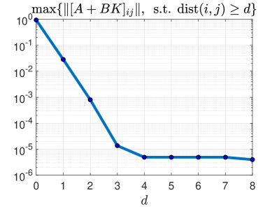
(a)

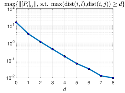
(b)

Figure 1: Spatial exponential decay of the closed-loop system in (a) and spatial exponential decay away from $i$ for $P_{i}$ that parameterizes the individual value function with $i=1$ in (b). In both (a) and (b) $K=-3I$ was used.

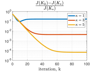
(a)

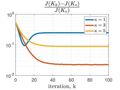
(b)

Figure 2: Relative cost of learned thermal controllers. In (a), the real, but truncated, $Q$-function was used. In (b) the $Q$-function was learned using $T_{c}=100,000$ samples.

Fig. 1 displays the spatial decay in the closed-loop system and corroborates Theorem 2 by illustrating how the individual value function also exhibits spatial exponential decay. Furthermore, Fig. 2 shows Algorithm 3’s performance in practice both when sampling the truncated Q-function and when using the real truncated Q-function. We note that when sampling the Q-function with $\kappa=3$, the algorithm performs better than with $\kappa=5$. In theory, this should not happen as the extra parameters introduced when using $\kappa=5$ always can be set to zero. This phenomenon stems from estimating the Q-function as it does not occur when using the real, truncated, Q-function (Fig. 2a). To mitigate this problem, more samples can be used in order to estimate the Q-function with higher accuracy.

VI Conclusions and Future Work

This paper concerns distributed learning of networked linear-quadratic controllers with decoupled costs and spatially exponentially decaying dynamics. We propose a scalable reinforcement learning algorithm that exploits the individual Q-functions’ spatially exponentially decaying structure and numerically test it on a thermal control problem.

There are several directions for future work. Most important is, perhaps, proving convergence of Algorithm 3 and stability of the resulting controllers. The question of sample complexity guarantees is also of interest. Finally, future work will include a practical evaluation of the algorithm through application to other problems in network learning and control.

-A Auxiliary lemmas: Properties of SED and SED away from $i$ matrices

Lemma 5

A $\kappa$-truncated controller, $K\in\mathcal{K}^{\kappa}$ is $(c_{K},\gamma)$-SED with $\gamma\in\mathbb{R}$ and $c_{K}:=\max_{ij}||[K]_{ij}||e^{\kappa\gamma}$.

Proof:

By definition, $||[K]_{ij}||=0$ when $j\notin\mathcal{N}_{i}^{\kappa}$ and for $j\in\mathcal{N}_{i}^{\kappa}$ it holds that

$$||[K]_{ij}||\leq\max_{ij}||[K]_{ij}||\leq\max_{ij}||[K]_{ij}||e^{\kappa\gamma}e^{-\gamma{\textnormal{dist}}(i,j)}$$

and the result follows immediately from the definition. ∎

Lemma 6

Suppose  $X,Y\in\mathbb{R}^{n\times m}$ are $(c_{x},\gamma_{x})$-SED and $(c_{y},\gamma_{y})$-SED, respectively, and let $\gamma=\min(\gamma_{x},\gamma_{y})$. Then, $X+Y$ is $(c_{x}+c_{y},\gamma)$-SED.

Proof:

$$\left\|[X+Y]_{ij}\right\|\leq\left\|[X]_{ij}\right\|+\left\|[Y]_{ij}\right\|\leq(c_{x}+c_{y})e^{-\gamma{\textnormal{dist}}(i,j)}\vspace{-2mm}$$

∎

Lemma 7 (Lemma 18 in [4])

Suppose $X\in\mathbb{R}^{n\times m}$, $Y\in\mathbb{R}^{m\times p}$ are $(c_{x},\gamma_{x})-SED$ and $(c_{y},\gamma_{y})-SED$, respectively, and let $\gamma=\min(\gamma_{x},\gamma_{y})$. Then, $XY$ is $(Nc_{x}c_{y},\gamma)-SED$.

Proof:

$$\left\|[XY]_{ij}\right\|=\left\|\sum_{r=1}^{N}[X]_{ir}[Y]_{rj}\right\|\leq\sum_{r=1}^{N}||[X]_{ir}||||[Y]_{rj}||$$

$$\leq\sum_{r=1}^{N}c_{x}c_{y}e^{-\gamma({\textnormal{dist}}(i,r)+{\textnormal{dist}}(r,j))}\leq\sum_{r=1}^{N}c_{x}c_{y}e^{-\gamma{\textnormal{dist}}(i,j)}$$

$$=Nc_{x}c_{y}e^{-\gamma{\textnormal{dist}}(i,j)}.$$

∎

Remark 3

By following the proofs of Lemma 6 and Lemma 7, it is easy to show that when $X$ and $Y$ are SED away from $i$ instead of SED, then $X+Y$, $XY$ are also SED away from $i$.

Another property of matrices that fulfill Definition 3 is that the decay away from $i$ is preserved when such a matrix is multiplied by a SED matrix.

Lemma 8

Let $Y\in\mathbb{R}^{n\times m}$ be $(c_{y},\gamma_{y})$-SED and let $X\in\mathbb{R}^{m\times p}$ be $(c_{x},\gamma_{x})$-SED away from i. Furthermore, let $\gamma=\min(\gamma_{x},\gamma_{y})$. Then $XY$ is $(Nc_{x}c_{y},\gamma)$-SED away from i.

Proof:

$$||[XY]_{lj}|| =\left|\left|\sum_{r=1}^{N}[X]_{lr}[Y]_{rj}\right|\right|\leq\sum_{r=1}^{N}||[X]_{lr}||\ ||[Y]_{rj}||$$

$$\leq\sum_{r=1}^{N}c_{x}c_{y}e^{-\gamma(\max({\textnormal{dist}}(i,l),{\textnormal{dist}}(i,r))+{\textnormal{dist}}(r,j))}$$

$$\leq Nc_{x}c_{y}e^{-\gamma\max({\textnormal{dist}}(i,l),{\textnormal{dist}}(i,j))}$$

Where we used $\max(a+c,b+c)\geq\max(a,b+c)\ \forall\ a,b,c\geq 0$ and the triangle inequality in the last step. ∎

Remark 4

It is easy to see that the bound in Lemma 8 also holds for the product $YX$, provided $X$ and $Y$ have suitable dimensions.

-B Proof of Lemma 1

Since $L$ is stable, the solution to the Lyapunov equation is unique and given by $P=\sum_{k=0}^{\infty}(L^{k})^{\top}ML^{k}$. Define $P^{t}$ to be the first $t$ terms in the series $P^{t}:=\sum_{k=0}^{t-1}(L^{k})^{\top}ML^{k}$. Then using that $L$ is $(\tau,\rho)$-stable,

$$\left\|P-P^{t}\right\|\!=\!\left\|\sum_{k=t}^{\infty}(L^{\top})^{k}ML^{k}\right\|\!\leq\!\sum_{k=t}^{\infty}||(L^{\top})^{k}||\ ||M||\ ||L^{k}||$$

$$\leq\!||M||\!\sum_{k=t}^{\infty}\!\tau^{2}\!e^{-2\rho k}\!=\!||M||\!\sum_{k=0}^{\infty}\!\tau^{2}\!e^{-2\rho(k+t)}\!=\!\frac{||M||\tau^{2}}{1-e^{-2\rho}}e^{-2\rho t}$$

Now since $L$ is $(c_{L},\gamma)$-SED, using some simple algebra on SED matrices (Lemma 7 in Appendix -A), $L^{k}$ is $(N^{k-1}c_{L}^{k},\gamma)$-SED and applying Lemma 8 twice, yields that $(L^{k})^{\top}ML^{k}$ is $((Nc_{L})^{2k}c_{M},\gamma)$-SED away from $i$. Furthermore, $c_{L}\geq 1~{}$ implies $(Nc_{L})^{2}\geq 2$ and thus

$$\sum_{k=0}^{t-1}(Nc_{L})^{2k}c_{M}=c_{M}\frac{(Nc_{L})^{2t}-1}{(Nc_{L})^{2}-1}\leq 2(Nc_{L})^{2(t-1)},$$

which means $P^{t}$ is $(2c_{M}(Nc_{L})^{2(t-1)},\gamma)$-SED away from $i$. Combining these results gives

$$\quad||[P]_{lj}||\leq||[P-P^{t}]_{lj}||+||[P^{t}]_{lj}||$$

$$\leq||P-P^{t}||+2c_{M}(Nc_{L})^{2(t-1)}e^{-\gamma\max(\text{dist}(i,l),\text{dist}(i,j))}$$

$$\leq\!\frac{||M||\tau^{2}}{1-e^{-2\rho}}e^{-2\rho t}\!+\!2c_{M}(Nc_{L})^{2(t-1)}e^{-\gamma\max(\text{dist}(i,l),\text{dist}(i,j))}.$$

This holds for any $t$, in particular it holds when the two terms are roughly equal. That is, for $t$ such that

$$e^{-2\rho t}=(Nc_{L})^{2(t-1)}e^{-\gamma\max({\textnormal{dist}}(i,l),{\textnormal{dist}}(i,j))}$$

and we therefore set

$$t=\left\lfloor\frac{\gamma\max({\textnormal{dist}}(i,l),{\textnormal{dist}}(i,j))}{2(\rho+\ln(Nc_{L}))}\right\rfloor+1,$$

which gives

$$||[P]_{lj}|| \leq\frac{||M||\tau^{2}}{1-e^{-2\rho}}e^{-2\rho t}+$$

$$2c_{M}(Nc_{L})^{2(t-1)}e^{-\gamma\max({\textnormal{dist}}(i,l),{\textnormal{dist}}(i,j))}$$

$$\leq\left(\frac{||M||\tau^{2}}{1-e^{-2\rho}}+2c_{M}\right)\times$$

$$\exp\left(-\frac{\rho\gamma}{\rho+\ln(Nc_{L})}\max({\textnormal{dist}}(i,l),{\textnormal{dist}}(i,j))\right).$$

$\hfill\blacksquare$

-C Proof of our main results: Theorem 2 and Corollary 3

We first prove the following helper lemma:

Lemma 9

Let $K$ be $(c_{K},\gamma_{sys})$-SED. Then, the matrix $S_{i}+[K]_{i:}^{\top}[R]_{ii}[K]_{i:}$ from the Lyapunov equation (2) is $(||[S]_{ii}||+||[R]_{ii}||c_{K}^{2},\gamma_{sys})$-SED away from i.

Proof:

First we note that

$$\left\|[[K]_{i:}^{\top}[R]_{ii}[K]_{i:}]_{lj}\right\|\leq||[R]_{ii}||c_{K}^{2}e^{-\gamma_{sys}{\textnormal{dist}}(i,l)}e^{-\gamma_{sys}{\textnormal{dist}}(i,j)}$$

and since $e^{-\gamma_{sys}{\textnormal{dist}}(i,l)}\leq 1$ for all $l$ we get

$$\left\|\![[K]_{i:}^{\top}\![R]_{ii}\![K]_{i:}]_{lj}\!\right\| \!\leq\!||\![R]_{ii}\!||c_{K}^{2}\!\min(e^{\!-\!\gamma_{sys}{\textnormal{dist}}(\!i,l\!)}\!,e^{\!-\!\gamma_{sys}{\textnormal{dist}}(\!i,j\!)}\!)$$

$$\!=\!||[R]_{ii}||c_{K}^{2}e^{-\gamma_{sys}\max({\textnormal{dist}}(i,l),{\textnormal{dist}}(i,j))}.$$

By construction of $S_{i}$, $[S_{i}]_{lj}=0$ unless $j=l=i$ and thus $S_{i}$ is $(||[S]_{ii}||,\gamma)$-SED away from $i$, for any $\gamma$. In particular it is true for $\gamma=\gamma_{sys}$. Combining these results using Lemma 6 into

$$||[S_{i}+[K]_{i:}^{\top}[R]_{ii}[K]_{i:}]_{lj}||\leq\\ (||[S]_{ii}||+||[R]_{ii}||c_{K}^{2})e^{-\gamma_{sys}\max({\textnormal{dist}}(i,l),{\textnormal{dist}}(i,j))}$$

finishes the proof. ∎

Theorem 2 and Corollary 3 now follows from Lemmas 1, 5, 6, 7 and 9.

Proof:

Lemma 5 gives that $K$ is $(c_{K},\gamma_{sys})$-SED. Lemma 6 and 7 then gives that $(A+BK)$ is $(c_{A}+Nc_{B}c_{K},\gamma_{sys})$-SED and Lemma 9 tells us the decay rate of $S_{i}+[K]_{i:}^{\top}[R]_{ii}[K]_{i:}$. The result directly follows by setting $L=(A+BK)$ and $M=S_{i}+[K]_{i:}^{\top}[R]_{ii}[K]_{i:}$ in Lemma 1. ∎

Proof:

The result follows immediately by applying Lemma 6 and 7 on the definition of the submatrices and then choosing $c_{H_{i}}$ as the maximum coefficient. ∎

-D Proof of Corollary 4

From the definition of $\underline{H}^{\kappa}_{i11}$ and Corollary 3 we have that $||[H_{i11}-\underline{H}^{\kappa}_{i11}]_{lj}||\leq c_{H_{i}}e^{-\gamma_{P_{i}}\kappa}.$ Multiplying by $x\in\mathbb{R}^{n}$ with $||x||=1$,

$$||[(H_{i11}-\underline{H}^{\kappa}_{i11})x]_{l}|| =\left|\left|\sum_{r=1}^{N}[(H_{i11}-\underline{H}^{\kappa}_{i11})]_{lr}x_{r}\right|\right|$$

$$\leq c_{H_{i}}e^{-\gamma_{P_{i}}\kappa}\sum_{r=1}^{N}||x_{r}||,$$

and thus

$$||(H_{i11}-\underline{H}^{\kappa}_{i11})x||^{2} \leq N(c_{H_{i}}e^{-\gamma_{P_{i}}\kappa})^{2}\left(\sum_{r=1}^{N}||x_{r}||\right)^{2}$$

$$\leq N(c_{H_{i}}e^{-\gamma_{P_{i}}\kappa})^{2}\sum_{r=1}^{N}||x_{r}||^{2}$$

$$=N(c_{H_{i}}e^{-\gamma_{P_{i}}\kappa})^{2}||x||^{2}.$$

Finally taking square roots on each side gives the result for $H_{i11}$. Repeating the same procedure for $H_{i12}$ and $H_{i22}$ finishes the proof. $\hfill\blacksquare$

References

• [1] B. Bamieh, F. Paganini, and M. Dahleh, “Distributed control of spatially invariant systems,” IEEE Transactions on Automatic Control, vol. 47, no. 7, pp. 1091–1107, 2002.
• [2] N. Motee and A. Jadbabaie, “Optimal control of spatially distributed systems,” IEEE Transactions on Automatic Control, vol. 53, no. 7, pp. 1616–1629, 2008.
• [3] S. Shin, Y. Lin, G. Qu, A. Wierman, and M. Anitescu, “Near-optimal distributed linear-quadratic regulator for networked systems,” SIAM Journal on Control and Optimization, vol. 61, no. 3, pp. 1113–1135, 2023.
• [4] R. Zhang, W. Li, and N. Li, “On the optimal control of network lqr with spatially-exponential decaying structure,” arXiv preprint arXiv:2209.14376, 2022.
• [5] S. Bradtke, “Reinforcement learning applied to linear quadratic regulation,” Advances in neural information processing systems, vol. 5, 1992.
• [6] S. J. Bradtke, B. E. Ydstie, and A. G. Barto, “Adaptive linear quadratic control using policy iteration,” in Proceedings of 1994 American Control Conference-ACC’94, vol. 3.   IEEE, 1994, pp. 3475–3479.
• [7] A. Lamperski, “Computing stabilizing linear controllers via policy iteration,” in 2020 59th IEEE Conference on Decision and Control (CDC), 2020, pp. 1902–1907.
• [8] K. Krauth, S. Tu, and B. Recht, “Finite-time analysis of approximate policy iteration for the linear quadratic regulator,” Advances in Neural Information Processing Systems, vol. 32, 2019.
• [9] M. Fazel, R. Ge, S. Kakade, and M. Mesbahi, “Global convergence of policy gradient methods for the linear quadratic regulator,” in International conference on machine learning.   PMLR, 2018, pp. 1467–1476.
• [10] Y. Abbasi-Yadkori, N. Lazic, and C. Szepesvári, “Model-free linear quadratic control via reduction to expert prediction,” in The 22nd International Conference on Artificial Intelligence and Statistics.   PMLR, 2019, pp. 3108–3117.
• [11] J. Bu, A. Mesbahi, M. Fazel, and M. Mesbahi, “Lqr through the lens of first order methods: Discrete-time case,” arXiv preprint arXiv:1907.08921, 2019.
• [12] G. Jing, H. Bai, J. George, A. Chakrabortty, and P. K. Sharma, “Learning distributed stabilizing controllers for multi-agent systems,” IEEE Control Systems Letters, vol. 6, pp. 301–306, 2021.
• [13] G. Qu, A. Wierman, and N. Li, “Scalable reinforcement learning for multiagent networked systems,” Operations Research, vol. 70, no. 6, pp. 3601–3628, 2022.
• [14] G. Qu, Y. Lin, A. Wierman, and N. Li, “Scalable multi-agent reinforcement learning for networked systems with average reward,” Advances in Neural Information Processing Systems, vol. 33, pp. 2074–2086, 2020.
• [15] Y. Zhang, G. Qu, P. Xu, Y. Lin, Z. Chen, and A. Wierman, “Global convergence of localized policy iteration in networked multi-agent reinforcement learning,” Proceedings of the ACM on Measurement and Analysis of Computing Systems, vol. 7, no. 1, pp. 1–51, 2023.
• [16] Y. Li, Y. Tang, R. Zhang, and N. Li, “Distributed reinforcement learning for decentralized linear quadratic control: A derivative-free policy optimization approach,” IEEE Transactions on Automatic Control, vol. 67, no. 12, pp. 6429–6444, 2021.
• [17] D. Görges, “Distributed adaptive linear quadratic control using distributed reinforcement learning,” IFAC-PapersOnLine, vol. 52, no. 11, pp. 218–223, 2019.
• [18] S. Alemzadeh and M. Mesbahi, “Distributed q-learning for dynamically decoupled systems,” in 2019 American Control Conference (ACC), 2019, pp. 772–777.
• [19] M. G. Lagoudakis and R. Parr, “Least-squares policy iteration,” The Journal of Machine Learning Research, vol. 4, pp. 1107–1149, 2003.
• [20] Olsson, Johan, “Scalable Reinforcement Learning for Linear-Quadratic Control of Networks,” 2023, M.Sc. Thesis, Lund University. [Online]. Available: http://lup.lub.lu.se/student-papers/record/9137268
• [21] D. Silver, G. Lever, N. Heess, T. Degris, D. Wierstra, and M. Riedmiller, “Deterministic policy gradient algorithms,” in International conference on machine learning.   Pmlr, 2014, pp. 387–395.
• [22] X. Zhang, W. Shi, X. Li, B. Yan, A. Malkawi, and N. Li, “Decentralized temperature control via HVAC systems in energy efficient buildings: An approximate solution procedure,” in 2016 IEEE Global Conference on Signal and Information Processing (GlobalSIP).   IEEE, 2016, pp. 936–940.