Bézier curves and the Takagi function

Abstract

We consider Bézier curves with complex parameter, and we determine explicitly the affine iterated function system (IFS) corresponding to the de Casteljau subdivision algorithm, together with the complex parametric domain over which such an IFS has a unique global connected attractor. For a specific family of complex parameter having vanishing imaginary part, we prove that the Takagi fractal curve is the attractor, under suitable scaling.

1 Introduction

In this paper we consider connections between a subdivision scheme of geometric modeling, the so-called de Casteljau algorithm for Bézier curves, and iterated function systems of fractal theory. We obtain an explicit representation of this algorithm as a pair of affine maps with coefficients in $\mathbb{Z}[t]$, the ring of polynomials in $t$ with integer coefficients. Here $t$ is the parameter of the Bézier curve, and fractals are obtained by allowing $t$ to assume complex values. After determining the range of $t$-values for which the IFS has a unique global connected attractor, we establish rigorously the appearance of the Takagi fractal curve in a specific asymptotic regime.

The Takagi curve is the graph of a continuous and nowhere differentiable function, the Takagi function, introduced by Teiji Takagi in 1903, and subsequently rediscovered several times, e.g., by Hildebrandt in 1933 or de Rham in 1957 [18]. It appears in many areas of mathematics, including analysis, probability theory, combinatorics, and number theory —see the surveys [1, 18] and references therein.

In geometric modelling, the recursive construction of fractals has proved valuable for generating realistic (i.e., typically non-smooth) forms. This approach originated from the work of Barnsley and co-workers on fractal image compression [3], using the machinery of iterated functions systems (IFS); these are dynamical systems consisting of collections of contraction mappings [2, section 3.7]. This idea later appeared in the context of subdivision schemes, such as Bézier and B–spline curves, which are widely used in geometric modeling, computer graphics, and computer aided design, due to the simplicity of their construction.

The first such application is due to R. Goldman [11], who presents a constructive procedure that builds an IFS based on the de Casteljau subdivision algorithm, and shows that Bézier curves are attractors of such an IFS.

Schaefer et al. [24] extend the idea by showing that curves and surfaces generated by several well-known subdivision algorithms are also attractors, fixed points of IFSs. They demonstrate how any curve generated by an arbitrary stationary subdivision scheme or subdivision surfaces without extraordinary vertices can be represented by an IFS. Furthermore, they provide a general paradigm for introducing control points and subdivision rules for arbitrary fractals generated by an IFS consisting of affine transformations, such as the Sierpinski gasket or the Koch curve. Moving the control points of these fractals induces transformations that are affine (but not necessarily conformal).

Tsianos and Goldman [25] study the somehow opposite direction: they show how to apply the de Casteljau subdivision algorithm and several standard knot insertion procedures for B-splines to build fractal shapes. They do so by allowing the parameters, or knots, to be complex numbers. Then they construct IFSs for these extended versions of classical subdivision algorithms, where the control points and the parameters are taken from the complex plane. They prove that starting with any control polygon, the IFS for Bézier curves with a given complex parameter converges uniformly to a limiting curve. Furthermore, they show that every fractal in the plane generated by a conformal IFS can be reproduced by Bézier subdivision in the complex plane [25, Corollary 3.3]. They can thus generate fractals with control points; however, in contrast to [24], adjusting the control points induces transformations that are conformal but not necessarily affine.

Some well-known subdivision schemes can also produce fractal curves and surfaces. For example, the four-point interpolating subdivision scheme introduced by Dyn et.al. [7] is defined using a tension parameter $\omega$, and the smoothness of the limit curves depends on such a parameter. Thus while the limit curve is almost $C^{2}$-continuous for some values of $\omega$, for other values one obtains fractal curves and surfaces, as shown in [13].

Connections between splines and fractals also emerge if one allows the order of a polynomial B-spline to be a real or complex number, leading to fractional and complex B-splines, respectively —see [10, 22] and references therein. The complexification of the order is also available for the so-called exponential B-splines, defined as convolution products of exponential functions, see [21, 22] and references therein. However, according to [22], neither the classical nor extended polynomial and exponential B-splines provide appropriate approximations of functions that exhibit self–similar or fractal behavior. In these cases, one needs to resort to fractal interpolation and approximation techniques. The extension of polynomial B-splines to self–similar or fractal functions was presented in [20] (see also [22, Section 5]).

The structure and main results of this paper are as follows. In section 2 we briefly review the theory of iterated function systems and deterministic fractals —the attractors of IFS that are the union of smaller copies of themselves. Alongside we provide the basic dynamical systems terminology, as well as some constructs and results on metric spaces and dimension. Our focus is on fractals generated by IFS consisting of affine transformations.

In section 3 we provide some background on Bézier curves, adopting the definition of the de Casteljau subdivision for curves with complex parameter $t$ and $n$ control points given in [24]. We then obtain an explicit representation of the de Casteljau scheme as a pair of affine maps on $\mathbb{Z}[t]^{n}$, and we determine the complex $t$-domain over which such an IFS has a unique connected attractor (theorem 3.2). This result rests on the key lemma 3.2, which provides a novel upper-triangular representation of the de Casteljau matrices.

In section 4 we consider the de Casteljau IFS, with two control points. For parameters of the type $t=1/2+\mathrm{i}\beta$ we associate to each binary code a curve —parametrised by $\beta$— that describes the location of the point with that symbolic address on the attractor. The derivative of these curves at $\beta=0$ define a vector field on the smooth Bézier curve, and we show that the Takagi function gives the amplitude of this field (lemma 4.4). Using this we then prove that a suitably scaled version of the attractor of the IFS in the $\beta\to 0$ limit is the Takagi curve (theorem 4.1). In the case of an arbitrary number of control points, the vector field has several components, and we show that one component is still given by the Takagi function (with a different scaling).

2 Iterated function systems

We provide some background on iterated function systems and related dynamical system terminology —see [2] and [16].

2.1 Dynamical systems preliminaries

Let $X$ be any set, and let $f:X\rightarrow X$ be a mapping. The $n$th iterate $f^{n}$ of $f$ is defined recursively as

$$f^{0}=\mathrm{Id}\hskip 30.0ptf^{n}=f\circ f^{n-1}\quad n>0,$$

and the sequence $(x_{n})_{n\geqslant 0}$ on $X$, where

$$x_{0}\in X\hskip 30.0ptx_{n}=f^{n}(x_{0})=f(x_{n-1})\quad n>0$$

is called the (forward) orbit through $x_{0}$.

A point $x\in X$ is said to be a fixed point of $f$ if $x=f(x)$. A closed set $A\subset X$ is an attractor for $f$ if $f(A)=A$ and there exists a neighborhood $U$ of $A$ and a positive integer $N$ such that $f^{N}(U)\subset U$ and

$$A=\bigcap_{n>0}f^{n}(U).$$

The set $U$ is called a fundamental neighborhood of $A$. Further, the open set

$$B=\bigcup_{n>0}(f^{n})^{-1}(U)$$

is called the basin of attraction of $A$.

We shall consider mostly linear mappings of $X=\mathbb{R}^{m}$, for which $f$ has the form $f(\mathbf{x})=\mathbf{M}\,\mathbf{x}$, with $\mathbf{M}$ a real $m\times m$ matrix. The orbits of this system are

$$\mathbf{x}_{0}=(x_{1},x_{2},\dots,x_{m})^{\top}\qquad\mathbf{x}_{n}=\mathbf{M}^{n}\mathbf{x}_{0}\qquad n>0.$$ (1)

The zero vector $\mathbf{x}^{\ast}=(0,\dots,0)^{{}^{\top}}$ is a fixed point of the mapping, and if $\mathbf{M}$ has a unit eigenvalue, then its entire eigenspace consists of fixed points.

If all eigenvalues of $\mathbf{M}$ lie inside the complex unit disc, then the powers $\mathbf{M}^{n}$ of $\mathbf{M}$ converge to zero matrix. Therefore, the sequence $\mathbf{x}_{n}$ converges to the zero vector for any $\mathbf{x}\in\mathbb{R}^{m}$, and thus the zero vector is an attractor with $\mathbb{R}^{m}$ as basin of attraction.

2.2 Complete metric spaces and iterated function systems

An iterated functions system is a dynamical system whose ‘points’ are subsets of a set, $\mathbb{R}^{m}$ in the present setting. The appropriate space for such a system is a complete metric space, namely a pair $(X,d)$, where $X$ is a set, and $d$ is a metric (i.e., a distance) on $X$ with respect to which all Cauchy sequences in $X$ converge to a limit in $X$.

Further, a mapping $f$ of $(X,d)$ to itself is a contraction mapping if there is a non-negative real number $s<1$ such that for all $x,y\in X$

$$d(f(x),f(y))\leqslant s\cdot d(x,y)\qquad 0\leqslant s<1.$$ (2)

The smallest such number $s$ is called the contractivity factor for $f$. The map $f$ is a contracting similarity if the leftmost equality holds in (2). Thus a linear contracting similarity transforms sets into geometrically similar sets.

The relevance of contraction mappings in our context is given by the Banach fixed point theorem [17, Section 5.1].

Theorem 2.1.

A contraction mapping of a complete metrix space has a unique fixed point. Such a fixed point is an attractor, whose basin of attraction is the whole space.

Fractals are compact sets, and we are interested in the set $\mathcal{H}(X)$ of all compact subsets of a set $X$. If $(X,d)$ is a complete metric space, one defines a metric $d_{H}$ on $\mathcal{H}(X)$ —the Haussdorf metric— which turns it into a complete metric space.

This is done as follows. Given $x\in X$ and $B\in\mathcal{H}(X)$, we define the distance from $x$ to $B$ as

$$d(x,B)=\min\{d(x,y)\,|\,y\in B\}.$$ (3)

Then, given $A\in\mathcal{H}(X)$ we define the distance from $A$ to $B$ as

$$d(A,B)=\max\{d(x,B)\,|\,x\in A\}.$$ (4)

Finally, by making the above symmetric, one obtains the Hausdorff metric $d_{H}$ on $\mathcal{H}(X)$:

$$\mathrm{d}_{H}(A,B)=\max\{d(A,B),d(B,A)\}.$$ (5)

The metric space $(\mathcal{H}(X),\mathrm{d}_{H})$ is complete [2, Section 7], and we now define a contraction mapping on $\mathcal{H}(X)$.

Definition.

Let $(X,d)$ be a complete metric space and let $f_{k}:X\rightarrow X,\;k=1,\dots N$ be a collection of contraction mappings with respective contractivity factors $s_{k}$. The dynamical system

$$F:\mathcal{H}(X)\rightarrow\mathcal{H}(X)\hskip 30.0ptF(A)=\bigcup_{k=1}^{N}f_{k}(A)$$ (6)

is called a (hyperbolic) iterated function system (IFS) on $X$.

Then we have [15]:

Theorem 2.2 (Hutchinson).

The transformation $F$ given in (6) is a contraction mapping on the complete metric space $(\mathcal{H}(X),\mathrm{d}_{H})$ with contractivity factor $s=\max\{s_{k}\;|\;k=1,\dots,N\}$.

From the above and Banach theorem 2.1, we conclude that $F$ has its unique fixed point $A^{\ast}\in\mathcal{H}(X)$, which obeys

$$A^{\ast}=F(A^{\ast})=\bigcup_{i=1}^{N}f_{k}(A^{\ast}),$$

and can be obtained as the limit

$$A^{\ast}=\lim_{n\rightarrow\infty}F^{n}(B)\hskip 5.0pt\text{for any}\hskip 5.0ptB\in\mathcal{H}(X).$$ (7)

The above fixed point will be called the attractor of the IFS. If $f_{k}$ are linear contracting similarities (see above), then the unique attractor $A$ is the union of smaller copies of itself.

Many well-known fractals are generated by affine iterated function systems. We consider maps of the form

$$f:\mathbb{R}^{m}\rightarrow\mathbb{R}^{m}\hskip 30.0ptf(\mathbf{x})=\mathbf{A}\mathbf{x}+\mathbf{b},$$ (8)

where $\mathbf{A}$ is an $m\times m$ regular matrix and $\mathbf{b}$ is $m$-dimensional vector. The fixed point $\mathbf{x}^{*}$ of $f$ is

$$\mathbf{x}^{\ast}=(\mathbf{I}-\mathbf{A})^{-1}\mathbf{b},$$

where $\mathbf{I}$ is the $m\times m$ identity matrix.

3 IFS for subdivision curves

Subdivision curves are defined recursively. The process starts with a given set of control points $\mathbf{P}^{k}$ as input, a refinement scheme is applied to them, generating as output a new refined set of control points $\mathbf{P}^{k+1}$. The subdivision curve is the limit of this recursive processs.

In [24, 25] a procedure is presented to generate an IFS for binary subdivision curves, including uniform B-spline curves and Bézier curves. We provide an alternative representation of the IFS of Bézier curves, and prove that in a suitable range of complex parameters this IFS is contractive and therefore has a unique fixed point, the global attractor. We also establish that in the same parametric domain the attractor is connected.

We first review some basic fact concerning Bézier curves.

3.1 Bézier Curves and the de Casteljau subdivision algorithm

Bézier curves were popularized in 1962 by the French engineer Pierre Bézier, who worked for Renault. They can be expressed explicitly as parametric curves using the Bernstein basis polynomials. Alternatively, points on a Bézier curve can be constructed by the de Casteljau algorithm, which was introduced by Paul de Casteljau already in 1959. He worked for Citroën and his work was kept a secret by Citroën for a long time [9]. P. de Casteljau and P. Bézier had different approach and they introduced Bézier curves independently, but P. Bézier could publish his work first.

The de Casteljau algorithm generalises to polynomial curves of arbitrary degree the construction of a parabola by repeated linear interpolation [8]. It is defined as follows: Let $\textbf{p}_{0},\dots,\textbf{p}_{n}\in\mathbb{R}^{3}$ be given set of control points and $t\in[0,1]$. We set

$$\left\{\begin{array}[]{rcl}\mathbf{p}_{i}^{0}(t)&=&\mathbf{p}_{i}\\ \mathbf{p}_{i}^{k}(t)&=&(1-t)\mathbf{p}_{i}^{k-1}(t)+t\mathbf{p}_{i+1}^{k-1}(t)\quad\left\{\begin{array}[]{rcl}k&=&1,\dots,n\\ i&=&0,\dots,n-k.\end{array}\right.\end{array}\right.$$ (9)

Then $\mathbf{p}_{0}^{n}(t)$ is the point with parameter value $t$ on the Bézier curve of degree $n$.

The de Casteljau algorithm can be viewed as a subdivision scheme, a method for finding new control points $\textbf{l}_{0}(t),\dots,\textbf{l}_{n}(t)$ and $\textbf{r}_{0}(t),\dots,\textbf{r}_{n}(t)$ from the original control points $\textbf{p}_{0},\dots,\textbf{p}_{n}$. These new control points, which represent the original Bézier curve restricted to the parameter intervals $[0,t]$ and $[t,1]$, respectively, are computed from the formulae

$$\begin{array}[]{ll}\textbf{l}_{i}(t)={\displaystyle\sum_{j=0}^{i}B_{j}^{i}(t)\textbf{p}_{j}},&i=0,\dots,n,\\ \textbf{r}_{i}(t)={\displaystyle\sum_{j=i}^{n}B_{n-j}^{n-i}(t)\textbf{p}_{i+n-j}},&i=0,\dots,n,\end{array}$$ (10)

where $B_{j}^{n}(t)$ are Bernstein basis polynomials $B^{n}_{j}(t)=\binom{n}{j}t^{j}(1-t)^{n-j}$.

The de Casteljau algorithm (10) can be rewritten into the following matrix form:

$$\begin{array}[]{rcl}\left(\begin{array}[]{c}\textbf{l}_{0}\\ \vdots\\ \textbf{l}_{n}\\ \end{array}\right)&=&\left(\begin{array}[]{cccc}B^{0}_{0}(t)&0&\ldots&0\\ B^{1}_{0}(t)&B_{1}^{1}(t)&\ldots&0\\ \vdots&\vdots&\vdots&\vdots\\ B^{n}_{0}(t)&B^{n}_{1}(t)&\ldots&B^{n}_{n}(t)\end{array}\right)\left(\begin{array}[]{c}\textbf{p}_{0}\\ \vdots\\ \textbf{p}_{n}\\ \end{array}\right)=\textbf{L}(t)\cdot\textbf{P}\\ {}\hfil&{}\hfil&{}\\ \left(\begin{array}[]{c}\mathbf{r}_{0}\\ \vdots\\ \mathbf{r}_{n}\\ \end{array}\right)&=&\left(\begin{array}[]{cccc}B^{n}_{0}(t)&B^{n}_{1}(t)&\ldots&B^{n}_{n}(t)\\ 0&B_{0}^{n-1}(t)&\ldots&B_{n-1}^{n-1}(t)\\ \vdots&\vdots&\vdots&\vdots\\ 0&0&\ldots&B_{0}^{0}(t)\end{array}\right)\left(\begin{array}[]{c}\mathbf{p}_{0}\\ \vdots\\ \mathbf{p}_{n}\\ \end{array}\right)=\textbf{R}(t)\cdot\textbf{P}\end{array}$$ (11)

The matrices $\textbf{L}(t)$, $\textbf{R}(t)$ represent the left and right subdivision scheme for Bézier curves. Starting with the original control points and applying these matrices repeatedly generates a sequence of control polygons that converge to the original Bézier curve.

The matrices $\textbf{L}(t)$ and $\textbf{R}(t)$ are invertible, with eigenvalues $\lambda_{i}=t^{i}$ and $\lambda_{i}=(1-t)^{i}$, respectively, for $i=0,\dots,n$. The eigenvector corresponding to $\lambda_{0}=1$ is $\mathbf{v}_{0}=(1,1,\dots,1)^{\top}$, since both matrices are row-stochastic.

3.2 IFS for Bézier curves with complex parameter

The de Casteljau algorithm (section 3.1) provides a subdivision scheme for Bézier curves with real parameter $t$. In order to generate fractals, we now extend it to the case of complex parameter $t\in\mathbb{C}$, and then transform the matrices $\mathbf{L}(t)$ and $\mathbf{R}(t)$ in $\mathbb{C}^{(n+1)\times(n+1)}$ into an IFS consisting of two affine maps $f_{0}$ and $f_{1}$ of $\mathbb{C}^{(n+1)}$, respectively.

This is achieved via a conjugacy that displays the $n$-dimensional linear part $\mathbf{A}_{k}$ and translation vector $\mathbf{b}_{k}$ of $f_{k}$ as sub-matrices —cf. equation (8). This may be done in four equivalent ways:

$$\begin{array}[]{cccc}\mathrm{I}&\quad\left(\begin{array}[]{cc}\mathbf{A}_{k}&\mathbf{b}_{k}\\ \mathbf{0}&1\end{array}\right)\hskip 60.0pt&\mathrm{II}&\quad\left(\begin{array}[]{cc}\mathbf{A}_{k}&\mathbf{0}\\ \mathbf{b}_{k}&1\end{array}\right)\\ \vskip 10.0pt\cr\mathrm{III}&\quad\left(\begin{array}[]{cc}1&\mathbf{b}_{k}\\ \mathbf{0}&\mathbf{A}_{k}\end{array}\right)\hskip 60.0pt&\mathrm{IV}&\quad\left(\begin{array}[]{cc}1&\mathbf{0}\\ \mathbf{b}_{k}&\mathbf{A}_{k}\end{array}\right)\end{array}\qquad k=0,1.$$ (12)

These matrices, which we shall call $\mathbf{M}^{(k)}$, $k=0,1$, are distinguished by the location of a row, or column, of the identity matrix $\mathbf{I}_{n+1}$. They act on the right (I and III) or on the left (II and IV), on column or row vectors that feature a 1 —the homogeneous component— in the last (I and II) or the first entry (III and IV).

The equivalence of these matrices is achieved by a combination of a reflection $(i,j)\leftrightarrow(n-i,n-j)$ and/or a transposition. The former is performed by the matrix with ones on the secondary diagonal (which coincides with its own inverse), while Theorem 1 of [26] guarantees the existence of a (symmetric) transposition similarity.

A general procedure for constructing a similarity between the de Casteljau matrices (11), or more general subdivision matrices, and the matrices $\mathbf{M}^{(k)}$ of type II was developed in [24]:

$$\mathbf{M}^{(0)}=\mathbf{P}^{-1}\;\mathbf{L}(t)\mathbf{P},\qquad\mathbf{M}^{(1)}=\mathbf{P}^{-1}\;\mathbf{R}(t)\mathbf{P},$$ (13)

where $\mathbf{P}$ is a square matrix created from any column vector whose last two entries differ (for instance, the vector of control points $(\mathbf{p}_{0},\dots,\mathbf{p}_{n})^{\top}\in\mathbb{C}^{(n+1)}$) by adding columns from identity matrix and a last column of ones corresponding to the homogenous component of the coordinates. The matrix $\mathbf{P}$, which performs a change of basis in $\mathbb{C}^{(n+1)\times(n+1)}$, is invertible by construction. We illustrate the effect of different choices of $\mathbf{P}$ on the attractor of IFS in Figure 1.

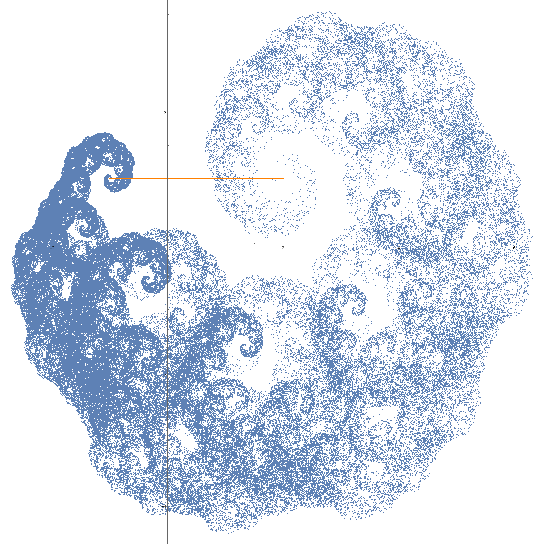
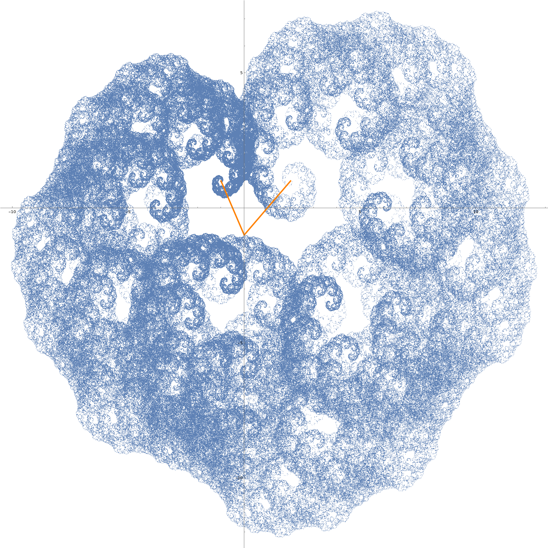
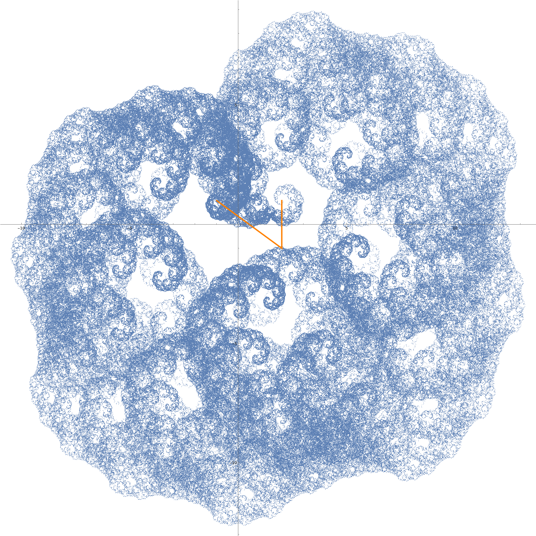
Figure 1: Attractors of IFS for quadratic Bézier curve with complex parameter $t=0.4-0.55i$ with control points (plotted as orange polyline) from left to right: $(-1+i,i,2+i)^{\top}$, $(-1+i,-i,2+i)^{\top}$, and $(-1+i,2-i,2+i)^{\top}$. The initial point $X\in\mathbb{C}^{1\times(n+1)}$ is an arbitrary point in dimension $n$ in homogenous coordinates. We show the state of the system after 20 iterations. In order to visualize the higher dimensional attractor, we project it to the complex plane. In all cases the fixed point of $f_{0}$ is the first row of matrix $\mathbf{P}$ of (13), i.e., $(-1+i,1,1)$, while the fixed point of $f_{1}$ is $(2+i,0,1)$ — the last row of $\mathbf{P}$.

Because the elements in a row of $\mathbf{L}(t)$ (and similarly for $\mathbf{R}(t)$) sum up to 1, and the last column of $\mathbf{P}$ is a column of ones, the last column of $\mathbf{L}(t)\mathbf{P}$ is also a column of ones. Further, the last column of $\mathbf{P}^{-1}\mathbf{L}(t)\mathbf{P}$ is the last column of the identity matrix $\mathbf{I}_{n+1}$ because the last column of $\mathbf{P}$ is a column of ones and $\mathbf{P}^{-1}\mathbf{P}=\mathbf{I}$. Thus the matrices $\mathbf{M}^{(k)}$ are both of type II in (12).

The great generality of the above construction is accompanied by a lack of specific information about the submatrices $\mathbf{A}_{k}$ and the translation vector $\mathbf{b}_{k}$ in $\mathbf{M}^{(k)}$. Below (theorem 3.2) we establish when the above affine IFS has a unique global connected attractor. For this purpose we must show that all infinite products of $\mathbf{A}_{0}$ and $\mathbf{A}_{1}$ converge to the zero matrix, or equivalently, that their joint spectral radius is less than one. Recall that the joint spectral radius of a set of matrices $\mathcal{A}$ is defined as

$$\rho(\mathcal{A}):=\lim_{n\to\infty}\sup\{||\mathbf{A}_{i_{1}}\cdots\mathbf{A}_{i_{n}}||^{\frac{1}{n}}:\mathbf{A}_{i}\in\mathcal{A}\},$$

where $||\cdot||$ is any matrix norm.

In the 90’s Daubechies and Lagarias [6] defined the generalized spectral radius, which was proved to be equal to the joint spectral radius for a bounded set of matrices [5]. The generalized spectral radius is defined as:

$$\rho(\mathcal{A}):=\lim_{n\to\infty}\sup\{\rho(\mathbf{A}_{i_{1}}\dots\mathbf{A}_{i_{n}})^{\frac{1}{n}},\mathbf{A}_{i}\in\mathcal{A}\}.$$

We shall employ the following lemma:

Lemma 3.1.

If $\mathbf{A}_{0},\mathbf{A}_{1}$ can be simultaneously upper-triangularized, i.e., if there exists an invertible matrix $\mathbf{S}$ such that $\mathbf{S}^{-1}\mathbf{A}_{0}\mathbf{S}$ and $\mathbf{S}^{-1}\mathbf{A}_{1}\mathbf{S}$ are both upper-triangular, then $\rho(\mathbf{A}_{0},\mathbf{A}_{1})=max\{\rho(\mathbf{A}_{0}),\rho(\mathbf{A}_{1})\}$.

Proof.

The result follows immediately from examination of the diagonal entries of the product of two upper-triangular matrices. See [12, Lemma 4.7]. ∎

Remark.

In [4] it is shown that a necessary and sufficient condition for a compact affine IFS in $\mathbb{R}^{n}$ to have a unique attractor is that $\rho(\mathcal{A})<1$, where $\mathcal{A}$ is the set of matrices corresponding to the linear part of the set of affine transformations the IFS consists of. This statement can be extended verbatim to our case of compact affine IFS in $\mathbb{C}^{n}$.

The next result, which is crucial to our analysis, exhibits a conjugacy that transforms $\mathbf{L}(t)$ into a diagonal matrix and $\mathbf{R}(t)$ into an upper-triangular matrix, both of type III in (12); these matrices are determined explicitly.

Lemma 3.2.

For any $n\geqslant 0$, let $\mathbf{S}$ be the matrix of eigenvectors of the $(n+1)\times(n+1)$ matrix $\mathbf{L}(t)$. Then $\mathbf{S}$ is invertible, and

$$\begin{array}[]{rcl}\displaystyle(\mathbf{S}^{-1}\mathbf{L}(t)\mathbf{S})_{i,j}&=&\displaystyle\binom{0}{i-j}t^{i}\\ \vskip 10.0pt\cr\displaystyle(\mathbf{S}^{-1}\mathbf{R}(t)\mathbf{S})_{i,j}&=&\displaystyle\binom{n-i}{n-j}t^{j-i}(1-t)^{i}\end{array}\hskip 30.0pti,j=0,\ldots,n.$$ (14)

Proof.

As noted above [see remarks after eq. (11)], the $(n+1)$-dimensional matrix $\mathbf{L}(t)$ over $\mathbb{Z}[t]$ has the $(n+1)$ distinct eigenvalues $t^{i}$, $i=0,\ldots,n$. Thus it is diagonalizable via the similarity $\mathbf{S}$, and considering that $\binom{0}{i-j}=\delta_{i,j}$, the Kronecker delta, the first formula in (14) is proved.

Next we show that $\mathbf{S}_{i,j}=\binom{i}{j}$, by computing the eigenvectors of $\mathbf{L}(t)$. We shall use the identity [14, p. 174]

$$\binom{i}{k}\binom{k}{j}=\binom{i}{j}\binom{i-j}{k-j}\qquad i,j,k\in\mathbb{Z}.$$ (15)

Keeping in mind the expression for $\mathbf{L}(t)$ in (11), and that $\mathbf{L}(t)_{i,k}=0$ for $k<0$ and $k>n$, we compute the $i$-th component of the $j$-th eigenvector by summing over all integers $k$. We obtain

$$\sum_{k}B^{i}_{k}\binom{k}{j} = \sum_{k}\binom{i}{k}\binom{k}{j}t^{k}(1-t)^{i-k}$$

$$= \binom{i}{j}\sum_{k}\binom{i-j}{k-j}t^{(k-j)+j}(1-t)^{(i-j)-(k-j)}$$

$$= t^{j}\binom{i}{j}\sum_{m}\binom{n}{m}t^{m}(1-t)^{n-m}$$

$$= t^{j}\binom{i}{j}(t+1-t)^{n}=t^{j}\binom{i}{j},$$

where the summation variable $m=k-j$ is unrestricted because $k$ is. The above shows that the $j$th column vector of $\mathbf{S}$ has components $\binom{i}{j},i=0,\ldots,n$, as desired.

Next we show that $\mathbf{S}^{-1}_{i,j}=(-1)^{i+j}\binom{i}{j}$, i.e., $\mathbf{S}^{-1}\mathbf{S}=\mathbf{I}$. Again, Using (15) and summing over $\mathbb{Z}$, we find:

$$\big{(}\mathbf{S}^{-1}\mathbf{S}\big{)}_{i,j}=\sum_{k}(-1)^{i+k}\binom{k}{j}=\binom{i}{j}(-1)^{i}\sum_{k}(-1)^{k}\binom{i-j}{k-j}.$$

If $i<j$ then $\binom{i}{j}=0$, and the rightmost expression above vanishes. The same happens if $j<i$, because in this case, from the binomial theorem, we have

$$\sum_{k}(-1)^{k}\binom{i-j}{k-j}=(-1)^{j}\sum_{m}\binom{i-j}{m}(-1)^{m}=(-1)^{j}(-1+1)^{i-j}=0.$$

Finally, for $i=j$ the only non-zero term in the sum corresponds to $k=i$, giving $\mathbf{S}^{-1}\mathbf{S}_{i,i}=\binom{i}{i}(-1)^{2i}=1$, as desired.

We have shown that the matrix product $\mathbf{S}^{-1}\mathbf{L}(t)\mathbf{S}$ is diagonal. It remains to show that $\mathbf{S}^{-1}\mathbf{R}(t)\mathbf{S}$ is upper-triangular. From the above and (11), we find:

$\mathbf{S}^{-1}\mathbf{R}(t)\mathbf{S}=\begin{pmatrix}1&0&\ldots&0\\ (-1)^{1}&(-1)^{1+1}\binom{1}{1}&\ldots&0\\ \vdots&\vdots&\vdots&0\\ (-1)^{n}&(-1)^{n+1}\binom{n}{1}&\ldots&(-1)^{n+n}\binom{n}{n}\\ \end{pmatrix}\begin{pmatrix}B^{n}_{0}(t)&B^{n}_{1}(t)&\ldots&B^{n}_{n}(t)\\ 0&B_{0}^{n-1}(t)&\ldots&B_{n-1}^{n-1}(t)\\ \vdots&\vdots&\vdots&\vdots\\ 0&0&\ldots&B_{0}^{0}(t)\\ \end{pmatrix}\begin{pmatrix}1&0&\ldots&0\\ 1&\binom{1}{1}&\ldots&0\\ \vdots&\vdots&\vdots&0\\ 1&\binom{n}{1}&\ldots&\binom{n}{n}\\ \end{pmatrix}$.

The explicit expression for the $(i,j)$-component $T^{(n)}_{i,j}$ of the matrix $\mathbf{S}^{-1}\mathbf{R}(t)\mathbf{S}$ is thus given by

$$T^{(n)}_{i,j} = \sum_{l=0}^{n}\sum_{k=0}^{n}(-1)^{i+l}\binom{i}{l}B^{n-l}_{k-l}(t)\binom{k}{j}$$ (16)

$$= \sum_{l}\sum_{k}(-1)^{i+l}\binom{i}{l}\binom{n-l}{k-l}\binom{k}{j}t^{k-l}(1-t)^{n-k},$$

where the summation ranges have been extended to $\mathbb{Z}$ because the binomial coefficients provide the stated restrictions. The above expression is a polynomial in $\mathbb{Z}[t]$.

Let us consider the sequence of matrices over $\mathbb{Z}[t]$:

$$\hat{T}^{(n)}_{i,j}=\binom{n-i}{n-j}t^{j-i}(1-t)^{i}\qquad n\geqslant 0,\quad i,j=0,\ldots,n.$$ (17)

We have $\hat{T}^{(0)}=(1)$, and for all $n>0$, $\hat{T}^{(n)}$ is upper triangular, with diagonal elements $\hat{T}^{(n)}_{i,i}=(1-t)^{i}$ (the eigenvalues of $\mathbf{R}(t)$).

We begin to show that the matrices $\hat{T}^{(n)}$ satisfy the identity

$$\hat{T}^{(n+1)}_{i+1,j+1}+\hat{T}^{(n+1)}_{i,j+1}=\hat{T}^{(n)}_{i,j+1}+\hat{T}^{(n)}_{i,j}\qquad n\geqslant 0,\quad i,j=0,\ldots,n.$$ (18)

Here we have included the value $j=n$ because from (17) we have $T^{(n)}_{i,n+1}=0$ for all $i$ (the lower index of the binomial coefficient is negative), even though this expression no longer represents a matrix element.

The left-hand side of (18) is given by

$$\hat{T}^{(n+1)}_{i+1,j+1}+\hat{T}^{(n+1)}_{i,j+1} = t^{j-i}(1-t)^{i}\left[\binom{n-i}{n-j}(1-t)+\binom{n+1-i}{n-j}t\right]$$

$$= t^{j-i}(1-t)^{i}\left[\binom{n-i}{n-j}+\binom{n-i}{n-j-1}t\right],$$

where we have used the binomial formula [14, p. 174]

$$\binom{n}{k}=\binom{n-1}{k}+\binom{n-1}{k-1}\qquad n,k\in\mathbb{Z}.$$ (19)

For the right-hand side of (18), we have

$$\hat{T}^{(n)}_{i,j+1}+\hat{T}^{(n)}_{i,j} = t^{j-i}(1-t)^{i}\left[\binom{n-i}{n-j-1}t+\binom{n-i}{n-j}\right],$$

which establishes (18).

Next we show —by double induction on $n$ and $i$— that the entries of $\hat{T}^{(n)}$ are uniquely determined by its first row $(i=0$) and column $(j=0)$. If $n=0$ this is trivially true, so assume that for some $n\geqslant 0$, the matrix $\hat{T}^{(n)}$ is known, and the first row and columns of $\hat{T}^{(n+1)}$ are also known. Then, from (18) we have that for all $j$ the sequence of equation

$$\hat{T}^{(n+1)}_{i+1,j+1}=-\hat{T}^{(n+1)}_{i,j+1}+\hat{T}^{(n)}_{i,j+1}+\hat{T}^{(n)}_{i,j},\qquad i=0,\ldots,n$$

may be solved recursively from the knowledge of the first term $\hat{T}^{(n+1)}_{0,j+1}$. One verifies that the above procedure accounts for all the missing entries of $\hat{T}^{(n+1)}$. [Recall the remark following (18).]

We shall now prove that $T^{(n)}_{i,j}$ in (16) is equal to $\hat{T}^{(n)}_{i,j}$, by showing that $T^{(0)}=\hat{T}^{(0)}$, and that for $n>0$ the matrices $T^{(n)}$ and $\hat{T}^{(n)}$ share the first row and column, and satisfy the same recursion formula (18).

We begin by computing the first row of $T^{(n)}$. For $i=0$, the term $\binom{i}{l}$ in (16) forces $l=0$, and hence using (15) and the binomial theorem, we find

$$T^{(n)}_{0,j} = \sum_{k}\binom{n}{k}\binom{k}{j}t^{k}(1-t)^{n-k}$$ (20)

$$= \binom{n}{j}\sum_{k}\binom{n-j}{k-j}t^{k+j-j}(1-t)^{n-k+j-j}$$

$$= \binom{n}{j}t^{j}\sum_{m}\binom{n-j}{m}t^{m}(1-t)^{n-j-m}$$

$$= \binom{n}{j}t^{j},\qquad n\geqslant 0,\quad i=0,\ldots,n,$$

which is (17) for $i=0$, as desired. This also shows that $T^{(0)}=(1)=\hat{T}^{(0)}$.

Next we compute the first column of $T^{(n)}$. For $j=0$, the binomial coefficient in (17) is zero unless also $i=0$, in which case it is equal to 1. We find

$$T^{(n)}_{i,0} = \sum_{l}(-1)^{i+l}\binom{i}{l}\sum_{k}\binom{n-l}{k-l}t^{k-l}(1-t)^{n-l+(k-l)}$$ (21)

$$= (-1)^{i}\sum_{l}(-1)^{l}\binom{i}{l}=\delta_{i,0},\qquad n\geqslant 0,\quad i=0,\ldots,n.$$

Indeed for $i>0$ the sum is zero, from the binomial theorem, while for $i=0$, we have $l=0$, hence $T^{n}_{0,0}=1$ (as above), which again agrees with (17) for $j=0$.

It remains to verify that $T$ satisfy (18). Using (15) twice, we find

$$T^{(n+1)}_{i+1,j+1} = \sum_{l}(-1)^{i+1+l}\binom{i+1}{l}\sum_{k}\binom{n+1-l}{k-l}\binom{k}{j+1}t^{k-l}(1-t)^{n+1-k}$$

$$= -\sum_{l}(-1)^{i+l}\binom{i}{l}\sum_{k}\binom{n+1-l}{k-l}\binom{k}{j+1}t^{k-l}(1-t)^{n+1-k}$$

$$+\sum_{l}(-1)^{i+(l-1)}\binom{i}{l-1}\sum_{k}\binom{n-(l-1)}{k-1-(l-1)}\left[\binom{k-1}{j+1}+\binom{k-1}{j}\right]$$

$$\hskip 50.0pt\times\,t^{k-l}(1-t)^{n-(k-1)}$$

$$= -T^{(n+1)}_{i,j+1}+T^{(n)}_{i,j+1}+T^{(n)}_{i,j}.$$

This establishes the identity

$$T^{(n+1)}_{i+1,j+1}+T^{(n+1)}_{i,j+1}=T^{(n)}_{i,j+1}+T^{(n)}_{i,j},$$

as desired. We remark that the above holds also for $j=n$, because in (16) we have $\binom{k}{n+1}=0$ for all $k$ for which $\binom{i}{l}\binom{n-l}{n-k}\not=0$, as easily verified. Hence $T^{(n)}_{i,n+1}=0=\hat{T}^{(n)}_{i,n+1}$.

We have shown that for all $n\geqslant 0$, the matrices $T^{(n)}$ and $\hat{T}^{(n)}$ have the same first row and column, and their entries satisfy the same recursion formula. Hence $T^{(n)}=\hat{T}^{(n)}$, for all $n$.

The proof of the lemma is complete. ∎

From the above result we obtain —as a bonus— the following identities for the double sums $T^{(n)}$, whose validity for $\hat{T}^{(n)}$ in (17) is verified at once.

Corollary.

Let $T^{(n)}_{i,j}$ be the sum (16). Then, for $n\geqslant 0$ and $j=0,\ldots,n$ the following holds:

$$\begin{array}[]{rcll}T^{(n)}_{i+1,j+1}&=&(1-t)\;T^{(n)}_{i,j}-t\;T^{(n)}_{i+1,j}&\quad i=0,\ldots,n-1\\ \vskip 5.0pt\cr T^{(n+1)}_{j+1,j+1}&=&(1-t)\;T^{(n)}_{i,j}&\quad i=0,\ldots,n.\end{array}$$

For our next result will shall need the following theorem [2, Chapter VIII, Theorem 2.1].

Theorem 3.1.

Let $\{f_{0},f_{1}\}$ be a hyperbolic IFS with attractor $\mathcal{A}$. Let $f_{0}$ and $f_{1}$ be one-to-one on $\mathcal{A}$. If

$$f_{0}(\mathcal{A})\cap f_{1}(\mathcal{A})=\emptyset,$$

then $\mathcal{A}$ is totally disconnected. If

$$f_{0}(\mathcal{A})\cap f_{1}(\mathcal{A})\neq\emptyset,$$

then $\mathcal{A}$ is connected.

Figure 2: The domain of $t$, over which is IFS $\{\mathbb{C};f_{1},f_{2}\}$ hyperbolic, is the intersection of two open discs $|t|<1$ and $|1-t|<1$.

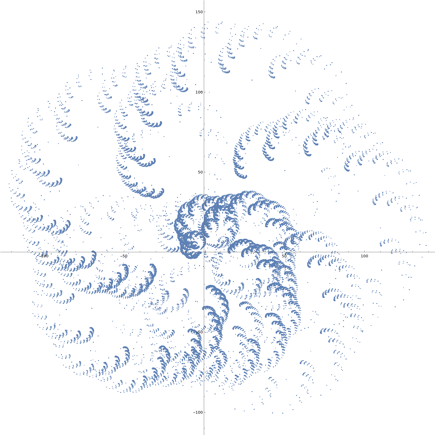
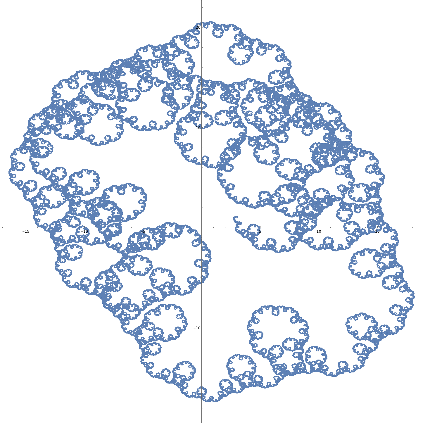
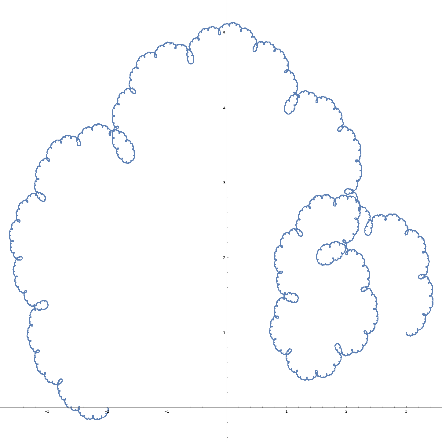
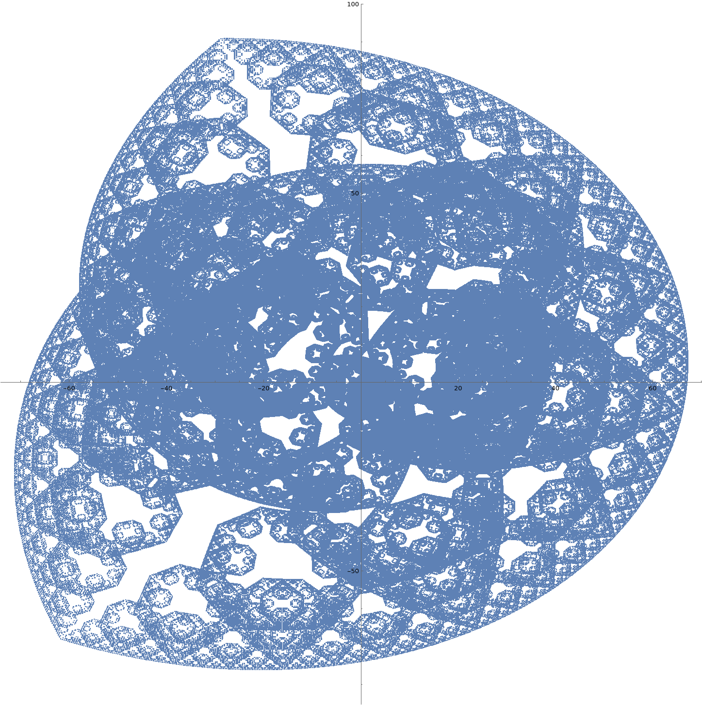
Figure 3: Attractor of IFS for Bézier curve of degree 6 with control points $(-2,-1+i,2i,1+i,1,2+i,3+i)^{\top}$ and complex parameters (from top to bottom and left to right): $t=0.1+0.3i$, $t=0.4+0.4i$, $t=0.5+0.25i$, and $t=0.5+0.5i$. We show the state of the system after 20 iterations, to visualize the higher dimensional attractor, we project it to the complex plane. Note that the fixed point of $f_{0}$ is the first row of matrix $\mathbf{P}$ of (13), i.e., $(-2,1,0,0,0,0,1)$, while the fixed point of $f_{1}$ is $(3+i,0,0,0,0,0,1)$ — the last row of $\mathbf{P}$.

We now show that the global attractor of the de Casteljau IFS for a complex Bézier curve is unique and connected. This is the main result of this section.

Theorem 3.2.

The affine IFS associated to the subdivision algorithm for a Bézier curve [as in (13) or (14)] has a unique and connected attractor for any parameter $t\in\mathbb{C}$ such that $|t|<1\wedge|1-t|<1$.

Proof.

From lemma 3.2 the similarity $\mathbf{S}$ transforms the de Casteljau matrices $\mathbf{L}(t)$ and $\mathbf{R}(t)$ to the form (12) III, moreover their $n\times n$ submatrices $\mathbf{A}_{0}$ and $\mathbf{A}_{1}$ are, respectively, diagonal and upper-triangular. Thus also $\mathbf{A}_{0}$ and $\mathbf{A}_{1}$ are simultaneously triangularizable, independently on the chosen representation from the list (12), since the change of representation can be achieved by a reflection $(i,j)\leftrightarrow(n-i,n-j)$ and/or a transposition —cf. discussion following table (12).

From lemma 3.1 we then have that

$$\rho(\mathbf{A}_{0},\mathbf{A}_{1})=\max\{\rho(\mathbf{A}_{0}),\rho(\mathbf{A}_{1})\}=\max\{|t|,|1-t|\}.$$

and hence in the domain $t\in\mathbb{C},\,|t|<1\wedge|1-t|<1$, all infinite products of the matrices $\mathbf{A}_{0}$ and $\mathbf{A}_{1}$ converge to the zero matrix, which ensures the contractivity of the IFS (in some metric). From Banach theorem 2.1 this IFS has a unique global attractor.

For computations we shall represent the IFS with the matrices

$$\mathbf{M}^{(0)}_{i,j}=\binom{0}{i-j}t^{i}\hskip 40.0pt\mathbf{M}^{(1)}_{i,j}=\binom{n-j}{n-i}t^{i-j}(1-t)^{j}\qquad i,j=0,\ldots,n.$$ (22)

of type IV in (12); these are the transposes of the matrices (14), and act on the right on $(n+1)$-dimensional column vectors representing homogeneous coordinates in $\mathbb{C}^{n}$.

Let $\{f_{0},f_{1}\}$ be the corresponding affine IFS. The maps $f_{0}$ and $f_{1}$, being affine, are one-to-one on the attractor $\mathcal{A}$, and in the assumed parameter range they are contractions, so their respective fixed points $z_{0}^{*}$ and $z_{1}^{*}$ belong to $\mathcal{A}$.

We claim that $z_{0}^{*}=(1,0^{m})^{\top}$ and $z_{1}^{*}=(\binom{n}{0},(\binom{n}{1},\ldots,\binom{n}{n})^{\top}$. The former is clear, since $\mathbf{M}^{(0)}$ is diagonal. As to the latter, using (15) and the binomial theorem, we find

$$(\mathbf{M}^{(1)}z_{1}^{*})_{i} = \sum_{j}\binom{n-j}{n-i}\binom{n}{j}t^{i-j}(1-t)^{j}$$

$$= \sum_{j}\binom{n}{n-j}\binom{n-j}{n-i}t^{i-j}(1-t)^{j}$$

$$= \binom{n}{n-i}\sum_{j}\binom{i}{i-j}t^{i-j}(1-t)^{j}=\binom{n}{i},$$

as desired. A straightforward calculation shows that $\mathbf{M}^{(0)}z_{1}^{*}=\mathbf{M}^{(1)}z_{0}^{*}$, both being equal to

$$\bigl{(}\binom{n}{0},t\binom{n}{1},\ldots,t^{n}\binom{n}{n}\bigr{)}^{\top}.$$

The above shows that $f_{0}(\mathcal{A})\cap f_{1}(\mathcal{A})\neq\emptyset$, and hence $\mathcal{A}$ is connected by theorem 3.1. ∎

The domain of $t$ over which the IFS has a unique global attractor is displayed in figure 2, while in figure 3 we show examples of the unique global attractor of the IFS, for a specific parameter value.

4 The Takagi curve

The Takagi curve is a graph of the Takagi (or Blancmange) function. Some of its remarkable properties are described in the surveys [1, 18]. It is defined by

$$\mathrm{T}(x)=\sum_{n=0}^{\infty}\frac{\sigma(2^{n}x)}{2^{n}}\qquad x\in[0,1]$$

where $\sigma(x)=\min_{n\in\mathbb{Z}}|x-n|$, that is, $\sigma(x)$ is the distance from $x$ to the nearest integer.

The Takagi curve has infinite length over any nonempty open interval in $[0,1]$ [18, Theorem 11.4], and it is self-similar in the sense that it satisfies a dyadic self-similarity equation [18, Theorem 4.1]. However, if we adopt Mandelbrot’s definition of a fractal as a set whose Hausdorff dimension is strictly greater than its topological dimension [19, p. 15], then the Takagi curve is not a fractal since its topological dimension and its Haussdorff dimension (as a subset of $\mathbb{R}^{2}$) are both equal to 1 [18, Theorem 11.2].

We shall prove that the Takagi curve represents the linearisation of the attractor of an IFS for a Bézier curve with complex parameter, as the parameter’s imaginary part goes to zero. We consider the de Casteljau algorithm for the Bézier curve with two control points, $0$ and $1$, in the complex plane. For real parameter $t$ the attractor $\mathcal{A}$ is a smooth curve connecting such points, but for complex $t$ the attractor is non-trivial. It is represented in homogeneous coordinates as the pair of complex matrices of type I in (12)

$$\mathbf{M}^{(0)}=\left(\begin{array}[]{cc}t&0\\ 0&1\end{array}\right)\hskip 30.0pt\mathbf{M}^{(1)}=\left(\begin{array}[]{cc}1-t&t\\ 0&1\end{array}\right).$$ (23)

The above matrices correspond to the pair of complex maps

$$f^{(0)}(z)=tz\qquad f^{(1)}(z)=(1-t)z+t.$$ (24)

We shall consider parameters of the form $t=1/2+\mathrm{i}\beta$, with real $\beta$. From theorem 3.2, for $|\beta|<\sqrt{3}/2$ the IFS is hyperbolic with a connected attractor $\mathcal{A}=\mathcal{A}(\beta)$. We then define the scaling map

$$\mathrm{g}:\mathbb{C}\times\mathbb{R}\to\mathbb{C}\qquad\mathrm{g}(z,\beta)=\operatorname{Re}(z)+\beta\,\mathrm{i}\,\operatorname{Im}(z)$$ (25)

together with the scaled attractor of the IFS:

$$\mathcal{A}^{*}(\beta)=\mathrm{g}(\mathcal{A}(\beta),(2\beta)^{-1}).$$ (26)

The properties of the scaled attractor depend strongly on $\beta$. In Figures 4–5 we plot $\mathcal{A}^{*}(\beta)$ of (26) for various values of $\beta$, and $\mathcal{T}$ for comparison. In all cases, the IFS is iterated 15 times, with the unit interval as initial set.

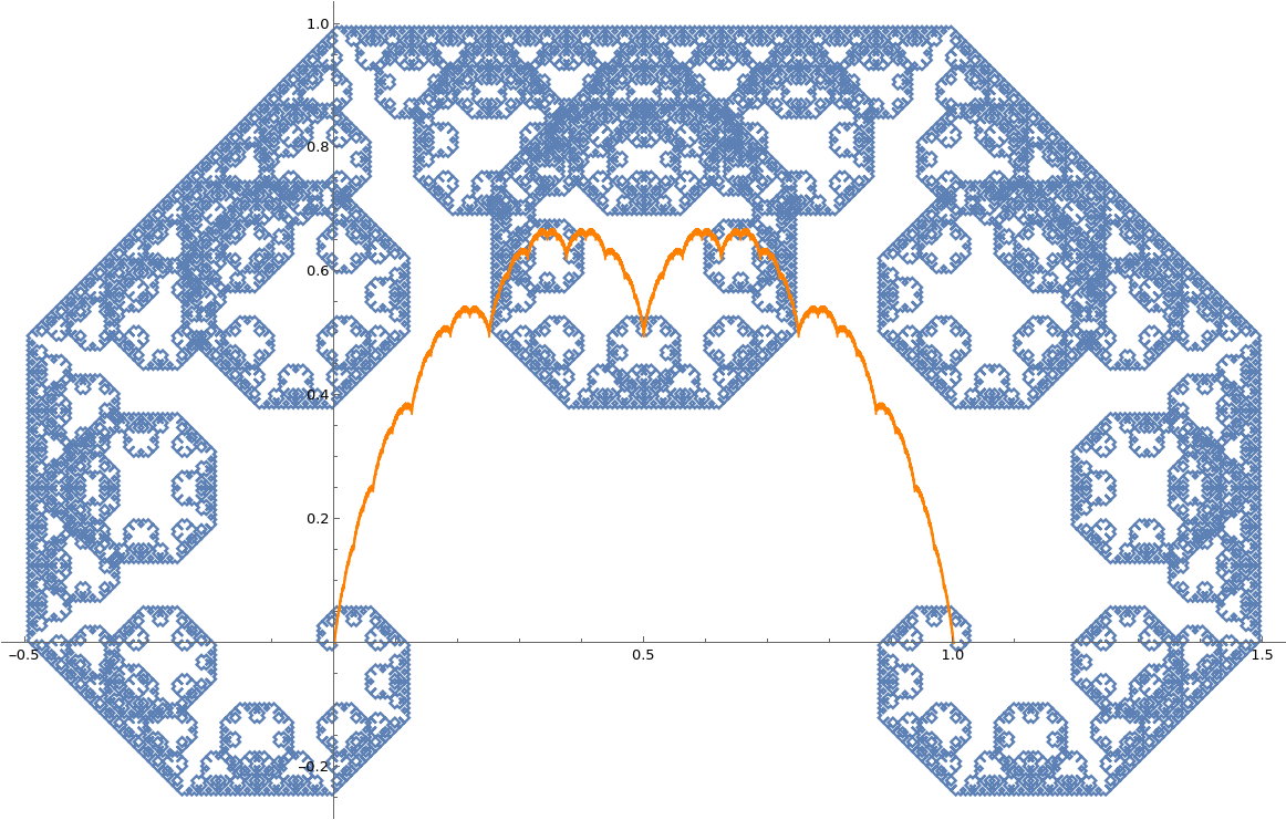
Figure 4: The blue curve is $\mathcal{A}^{\ast}(\beta)$, which for $\beta=\frac{1}{2}$ becomes the Lévy C curve. The orange curve is the graph $\mathcal{T}$ of the Takagi function $\mathrm{T}$.

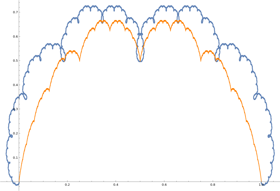
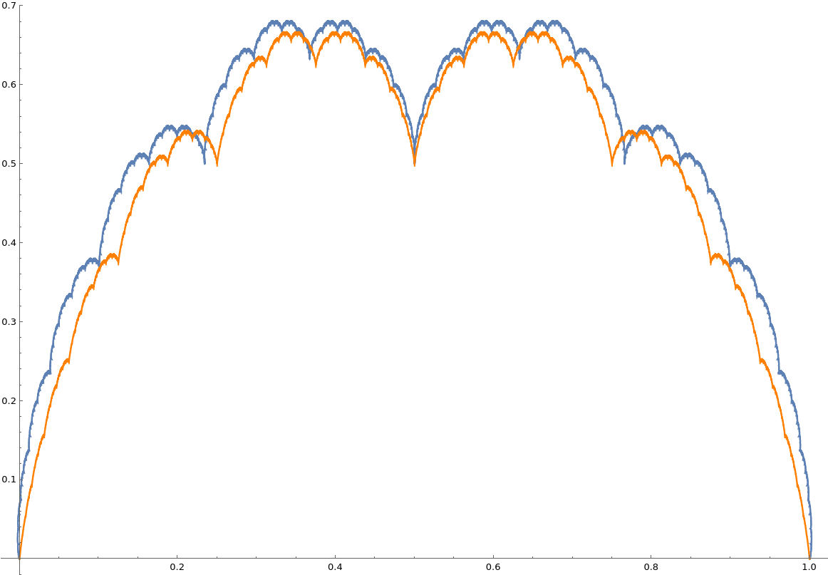
Figure 5: Left: the scaled attractor $\mathcal{A}^{\ast}(\beta)$ for $\beta=\frac{1}{4}$ (blue) and the Takagi curve (orange). Right: the same for $\beta=\frac{1}{8}$. For $\beta=\frac{1}{4}$, the attractor features crunodes; these appeared to have turned into cusps for $\beta=\frac{1}{8}$, although this is not the case (see remark after theorem 4.1).

We begin our analysis of this class of phenomena. Let $\Omega=\{0,1\}^{\mathbb{N}}$ be the space of infinite binary sequences. Any $d\in\Omega$ represents the digits of a real number $x^{(d)}\in[0,1]$. Since the elements of $\mathbb{Z}[1/2]$ are precisely the real numbers that admit two distinct binary representations, for uniqueness we shall stipulate that these digits must eventually be all zeros rather than all ones, with the exception of $d=(1^{\infty})$. With this provision the map

$$\pi:\Omega\to[0,1]\hskip 30.0ptd\mapsto x^{(d)}=\sum_{k=1}^{\infty}\frac{d_{k}}{2^{k}}$$ (27)

is a bijection, and we shall speak of convergence and measure in $\Omega$ in terms of the distance and Lebesgue measure in the unit interval. Note that $d$ is eventually periodic iff $x^{(d)}\in\mathbb{Q}$.

Next we define the operator that reverses the first $n$ terms of a sequence: For every $d=(d_{1},d_{2},\ldots)\in\Omega$ and $n\in\mathbb{N}$ we let

$$\overleftarrow{d}\hskip-1.0pt(n):=(d_{n},d_{n-1},\ldots,d_{1},0^{\infty}).$$ (28)

From our convention on digits it follows that $\lim_{n\to\infty}\overleftarrow{d}\hskip-1.0pt(n)=(0^{\infty})$ iff $x^{(d)}$ is a dyadic rational.

For any sequence $d$ we define

$$r_{n}^{(d)}=\sum_{k=1}^{n}\frac{d_{k}}{2^{k}}\hskip 30.0ptu_{n}^{(d)}=\sum_{k=1}^{n}d_{k}.$$ (29)

Thus $r_{n}$ is the rational number whose binary digits are $d(n)$ and $u_{n}^{(d)}$ is the number of ones in $d(n)$. Plainly,

$$\lim_{n\to\infty}r_{n}^{(d)}=x^{(d)}.$$ (30)

Further, given $d$, we define the matrix product

$$\mathbf{M}_{n}(d)=\mathbf{M}^{(d_{1})}\mathbf{M}^{(d_{2})}\dots\mathbf{M}^{(d_{n})},$$ (31)

this corresponds to the affine map

$$f_{n}^{(d)}=f^{(d_{1})}\circ f^{(d_{2})}\circ\cdots\circ f^{(d_{n})}$$ (32)

This map performs $n$ iterates, selecting the map $f_{k}$ according to the digit $d_{k}$ in reverse order, that is, the symbolic sequence that defines $f^{(d)}$ is $\overleftarrow{d}\hskip-1.0pt$. (The reason for this unconventional choice will become clear below.)

The map $f$, being a composition of affine maps, is affine, and an easy induction shows that it has the form

$$f_{n}^{(d)}(z)=U_{n}^{(d)}z+Z_{n}^{(d)}\qquad U_{n}^{(d)}=(1-t)^{u_{n}}t^{n-u_{n}},$$ (33)

where $Z_{n}^{(d)}$ is a polynomial in $t$.

We now specialise to parameters of the form $t=1/2+\mathrm{i}\beta$, with real $\beta$. We choose $z=0\in\mathcal{A}$ as the initial point of the orbit. From (33) we obtain

$$f_{n}^{(d)}(0)=Z_{n}^{(d)},$$ (34)

and from (24) we see that $Z_{n}^{(d)}$ is a polynomial in $\mathrm{i}\beta$ with coefficients in $\mathbb{Z}[1/2]$, the set of rational numbers whose denominator is a power of 2. Writing

$$Z_{n}^{(d)}=\sum_{k\geqslant 0}a_{k,n}^{(d)}(\mathrm{i}\beta)^{k}=X_{n}^{(d)}+\mathrm{i}Y_{n}^{(d)},\qquad a_{k,n}\in\mathbb{Z}[1/2],$$ (35)

we find that $X_{n}^{(d)}$ and $Y_{n}^{(d)}$ are real polynomials that correspond, respectively, to the even and odd powers of $\beta$.

Lemma 4.1.

The polynomials $Z_{n}^{(d)}$ of (34) satisfy the recursion relation

$$Z_{0}^{(d)}=0\hskip 30.0ptZ_{n+1}^{(d)}=\begin{cases}Z_{n}^{(d)}&d_{n+1}=0\\ Z_{n}^{(d)}+W_{n}^{(d)}&d_{n+1}=1\end{cases}$$ (36)

where

$$W_{n}^{(d)}(\beta)=\sum_{m\geqslant 0}w_{m,n}\beta^{m}\hskip 30.0ptw_{m,n}=\frac{\mathrm{i}^{m}}{2^{n+1-m}}\sum_{k=0}^{m}(-1)^{k}\binom{u_{n}}{k}\binom{n+1-u_{n}}{m-k}.$$ (37)

Proof.

We proceed by induction on $n$. For $n=0$ from (32) we have

$$Z^{(d)}_{1}=\begin{cases}0&d_{1}=0\\ \frac{1}{2}+\mathrm{i}\beta&d_{1}=1.\end{cases}$$

so formula (36) holds in the case $d_{1}=0$. If $d_{1}=1$, then the sums (37) with $n=u_{n}=0$ are restricted to $k=0$ and $m=0,1$, for which all binomial coefficients are 1. We find $w_{0,0}=1/2$ and $w_{1,0}=\mathrm{i}$, in accordance with (36).

Assume now that (36) and (37) hold for some $n\geqslant 1$. We have two cases. If $d_{n+1}=0$, then from (24) we have $f_{d_{n+1}}(0)=0$, that is, the first iterate of the map doesn’t change the initial point. Hence, from (34) we have $Z_{n+1}^{(d)}=Z_{n}^{(d)}$, so that

$$a_{k,n+1}=a_{k,n}\quad k=0,1,\ldots\hskip 30.0pt(d_{n+1}=0),$$ (38)

in accordance with (35) and (36).

If $d_{n+1}=1$, then we have $f_{d_{n+1}}(0)=t$ and from (33) we have

$$Z_{n+1}^{(d)}=f_{n+1}^{(d)}(0)=f_{n}^{(d)}(t)=U_{n}^{(d)}t+Z_{n}^{(d)}.$$ (39)

Letting $W_{n}^{(d)}=U_{n}^{(d)}t$ with $t=1/2+\mathrm{i}\beta$ and using the binomial theorem, we find

$$W_{n}^{(d)} = (1/2-\mathrm{i}\beta)^{u_{n}}(1/2+\mathrm{i}\beta)^{n-u_{n}+1}$$ (40)

$$= \left(\sum_{k}\binom{u_{n}}{k}(-1)^{k}(\mathrm{i}\beta)^{k}\frac{1}{2^{u_{n}-k}}\right)\times\left(\sum_{\ell}\binom{n-u_{n}+1}{\ell}(\mathrm{i}\beta)^{\ell}\frac{1}{2^{n-u_{n}+1-\ell}}\right)$$

$$= \sum_{k}(-1)^{k}\binom{u_{n}}{k}\sum_{\ell}\binom{n-u_{n}+1}{\ell}\frac{1}{2^{n+1-k-\ell}}(\mathrm{i}\beta)^{k+\ell}.$$

Letting $k+\ell=m$ in (40) we obtain

$$w_{m,n}=\frac{\mathrm{i}^{m}}{2^{n+1-m}}\sum_{k}(-1)^{k}\binom{u_{n}}{k}\binom{n+1-u_{n}}{m-k}.$$

For $k<0$ ($k>m$) the first (second) binomial coefficient is zero, so we may restrict the range of summation to $0\leqslant k\leqslant m$, which completes the proof of the recursion formulae. ∎

Lemma 4.2.

Let $(a_{k,n}^{(d)})$ be the coefficients of $Z_{n}^{(d)}$, as in lemma 4.1. Then for all $d$ and $k$ the following limit exists

$$a_{k}^{(d)}:=\lim_{n\to\infty}a_{k,n}^{(d)},\qquad\mbox{with the bound }\qquad|a_{k}^{(d)}|<2^{k+1}$$ (41)

independent on $d$. Thus the polynomials $Z_{n}^{(d)}$ converge coefficientwise to a convergent power series:

$$Z^{(d)}(\beta):=\lim_{n\to\infty}Z_{n}^{(d)}(\beta),\qquad|\beta|<\frac{1}{2}.$$ (42)

Proof.

Using the identities [14, pp 174,199]

$$\sum_{k}\binom{r}{k}\binom{s}{m-k}=\binom{r+s}{m},\hskip 30.0pt\frac{z^{m}}{(1-z)^{m+1}}=\sum_{k\geqslant 0}\binom{k}{m}z^{k}\quad(m\geqslant 0),$$

and formula (37) we obtain the following uniform bound

$$|a_{m,n+1}| = |a_{m,n+1}-a_{m,0}|=\left|\sum_{j=0}^{n}(a_{m,j+1}-a_{m,j})\right|$$

$$\leqslant \sum_{j=0}^{n}\bigl{|}a_{m,j+1}-a_{m,j}\bigr{|}=\sum_{j=0}^{n}|w_{m,j}|$$

$$= \sum_{j=0}^{n}\frac{2^{m}}{2^{j+1}}\sum_{k}\binom{u_{j}}{k}\binom{j+1-u_{j}}{m-k}$$

$$= 2^{m}\sum_{j=0}^{n}\frac{1}{2^{j+1}}\binom{j+1}{m}$$

$$< 2^{m}\sum_{j=0}^{\infty}\frac{1}{2^{j+1}}\binom{j+1}{m}=2^{m+1}.$$

The above derivation shows that, for all $d\in\Omega$, the series $\sum_{j}w_{m,j}$ converges absolutely, which implies that, as $n\to\infty$, of the sequence of polynomials $Z_{n}^{(d)}$ converge coefficientwise to a power series; the latter in turn converges for $|\beta|<1/2$ for all $d$. ∎

We shall use the following lemma (see [1, p. 19]).

Lemma 4.3.

For any sequence $d\in\Omega$ let $r_{n}^{(d)}$ and $u_{n}^{(d)}$ be as in (29), and let $\mathrm{T}$ be the Takagi function. Then for any $m\geqslant n$ we have

$$\mathrm{T}\big{(}r_{n}^{(d)}+\frac{1}{2^{m}}\big{)}-\mathrm{T}\big{(}r_{n}^{(d)}\big{)}=\frac{m-2u_{n}^{(d)}}{2^{m}}.$$ (43)

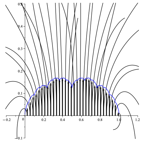
Figure 6: The parametric curves $Z_{n}^{(d)}(\beta)$ of (34) in the complex plane, for all binary sequences of length $n=2^{6}$, and $\beta\in[0,1/4]$. The arrow tangent to each curve at $\alpha=Z_{n}^{(d)}(0)$ represents the vector field $\mathbf{v}(\alpha)$ scaled by the value $\beta=1/8$, which is a linear approximation of the attractor $\mathcal{A}(1/8)$ (the transversal curve). Intersections of parametric curves correspond to the appearance of points with multiple addresses in the attractor.

The connection between Bézier curves and the Takagi function first appears in the following result.

Lemma 4.4.

Let $Z^{(d)}$ be as in (42). Then, for every $\alpha\in[0,1]$ we have

$$\mathbf{v}(\alpha):=\left.\frac{\mathrm{d}Z^{(\pi^{-1}(\alpha))}(\beta)}{\mathrm{d}\beta}\right|_{0}=2\mathrm{i}\mathrm{T}(\alpha),$$ (44)

where $\pi$ was defined in (27) and $\mathrm{T}$ is the Takagi function.

Proof.

From lemma 4.1 we have

$$\left.\frac{\mathrm{d}Z_{n}^{(d)}(\beta)}{\mathrm{d}\beta}\right|_{0}=\mathrm{i}a_{1,n}^{(d)}$$

so we have to compute the limits $a_{0}^{(d)}$ and $a_{1}^{(d)}$ as in (41). We determine the first coefficient $a_{0,n}$ of the polynomial $Z_{n}^{(d)}$.

If $\beta=0$, the IFS (24) is represented as the pair of planar maps

$$F_{0}(x,y)=\bigl{(}\frac{1}{2}x\,,\,\frac{1}{2}y\bigr{)}\hskip 30.0ptF_{1}(x,y)=\bigl{(}\frac{1}{2}x+\frac{1}{2}\,,\,\frac{1}{2}\bigr{)}.$$ (45)

The attractor $\mathcal{A}(0)$ is the unit interval, over which the map is seen to be the inverse of the doubling map $x\mapsto 2x\,({\rm mod\ }1)$. Let $d(n)=(d_{1},d_{2},\ldots,d_{n})$ be the sequence of the first $n$ digits of $d$, and consider expression (33) for the finite sequence $\overleftarrow{d}\hskip-1.0pt(n)$. Since $\beta=0$, the final point will be $Z_{n}^{(d)}(0)=a_{0,n}$, where $a_{0,n}$ is a rational number.

Now, the symbolic dynamics of the orbit of (33) with initial condition at 0 is $\overleftarrow{d}\hskip-1.0pt(n)$, and therefore the symbolic itinerary of its inverse —the doubling map— is $d(n)$. Since the latter is just the binary expansion of the initial point, we have

$$a_{0,n}=r_{n}^{(d)}=\sum_{k=1}^{n}\frac{d_{k}}{2^{k}}\,\in\,\mathbb{Z}[1/2],$$ (46)

that is, the dyadic rational $r_{n}^{(d)}$ is the initial point of an eventually periodic orbit of the doubling map, which terminates at the fixed point $0$ in $n$ steps. From (46) we have

$$a_{0,n+1}=\begin{cases}a_{0,n}&d_{n+1}=0\\ a_{0,n}+\frac{1}{2^{n+1}}&d_{n+1}=1.\end{cases}$$

Our claim now follows from (30).

Next we determine $a_{1,n}$, using induction on $n$. For $n=1$ we have $f^{(0)}(0)=0$ and $f^{(1)}(0)=1/2+\mathrm{i}\beta=a_{0,1}+\mathrm{i}\beta a_{1,1}$, so in either case we have $a_{1,1}=2\mathrm{T}(a_{0,1})$. Assume now that this is true for all binary sequences of length $n$: $a_{1,n}=2\mathrm{T}(a_{0,n})$.

We consider the successive digit $d_{n+1}$. If $d_{n+1}=0$ we have $a_{1,n+1}=a_{1,n}$ from (38), and there is nothing to prove. If $d_{n+1}=1$, then from (36) and (37) with $m=1$ we find

$$a_{1,n+1}=-\mathrm{i}w_{1,n}+a_{1,n}.$$ (47)

We compute

$$-\mathrm{i}w_{1,n}=\frac{1}{2^{n}}[(n+1-u_{n})-u_{n}]=\frac{n+1-2u_{n}}{2^{n}}.$$

From the above, equation (47), the induction hypothesis, and lemma 4.3 with $m=n+1$, we have

$$a_{1,n+1}=a_{1,n}+\frac{n+1-2u_{n}}{2^{n}}=\mathrm{T}(a_{0,n})+\frac{n+1-2u_{n}}{2^{n}}=2\mathrm{T}\bigl{(}a_{0,n}+\frac{1}{2^{n+1}}\bigr{)},$$

which completes the induction. Taking the limit, we have, for any $d$

$$\lim_{n\to\infty}a_{1,n+1}^{(d)}=\lim_{n\to\infty}2\mathrm{T}\bigl{(}a_{0,n}^{(d)}+\frac{d_{n+1}}{2^{n+1}}\bigr{)}=2\mathrm{T}(\lim_{n\to\infty}a_{0,n+1}^{(d)})=2\mathrm{T}(x^{(d)}),$$

the penultimate step being justified by the continuity of $\mathrm{T}$. The proof is complete. ∎

From lemmas 4.2 and 4.4 we obtain an infinite sequence of functions

$$a_{k}:[0,1]\to\mathbb{R}\qquad\alpha\mapsto a_{k}^{(\pi^{-1}(\alpha))}\qquad k=0,1,\ldots,$$ (48)

with $a_{0}(\alpha)=\alpha$, $a_{1}(\alpha)=2\mathrm{T}(\alpha)$, and $a_{k}$ displaying an increasing degree of irregularity as $k$ increases (see figure 7).

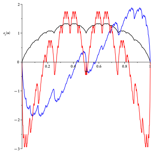
Figure 7: The graphs of the functions $\alpha\mapsto a_{k}(\alpha)$ of (48), for $k=1$ (black), $k=2$ (blue) and $k=3$ (red). The function $a_{1}$ is the scaled Takagi function —cf. lemma 4.4.

The quantity $\mathbf{v}$ is the simplest instance of a non-smooth vector field on a smooth Bézier curve $\mathcal{B}=\mathcal{A}(0)$ (see figure 6). The field $\mathbf{v}$ is orthogonal to the curve, and arises from the complexification of the curve’s parameter: $t=1/2+\mathrm{i}\beta$. In this context the function $\mathrm{g}$ performs scaling in the direction of the vector field.

The set

$$\bigcup_{\alpha}\bigl{(}\alpha+\mathbf{v}(\alpha)\beta\bigr{)},$$

represents a linear approximation of $\mathcal{A}(\beta)$ (see figure 6), which improves as $\beta\to 0$. To express this fact more precisely, we scale $\mathcal{A}$ in the direction of the field. This is the content of the following theorem.

Theorem 4.1.

Let $\mathcal{A}(\beta)\in\mathbb{C}$ be the attractor of the de Casteljau IFS (24) for the Bézier curve with control points $0$ and $1$ and complex subdivision parameter $t=\frac{1}{2}+i\beta$, and $\mathrm{g}$ the scaling map (25). Then

$$\lim_{\beta\to 0}\mathrm{d}_{H}(\mathrm{g}\big{(}\mathcal{A}(\beta),(2\beta)^{-1}\big{)},\mathcal{T})=0,$$ (49)

where $\mathcal{T}$ is the graph of the Takagi function and $\mathrm{d}_{H}$ is the Hausdorff distance (5).

Proof.

We shall provide two proofs.

From lemma 4.2, we can represent the attractor of the IFS as

$$\mathcal{A}(\beta)=\bigcup_{d\in\Omega}Z^{(d)}(\beta)=\bigcup_{\alpha\in[0,1]}Z^{(\pi^{-1}(\alpha))}(\beta)\qquad\beta<1/2.$$

Let $\mathcal{A}^{*}(\beta)=\mathrm{g}(\mathcal{A}(\beta),(2\beta)^{-1})$, and write $Z(\alpha,\beta)$ for $Z^{(\pi^{-1}(\alpha)}(\beta)$. We have

$$\mathcal{A}^{*}(\beta) = \bigcup_{\alpha}\mathrm{g}(Z(\alpha,\beta),(2\beta)^{-1})=\bigcup_{\alpha}\alpha+\mathrm{g}(Z(\alpha,\beta)-\alpha,(2\beta)^{-1})$$

$$= \bigcup_{\alpha}\alpha+\frac{1}{2}\mathbf{v}(\alpha)+O_{\alpha}(\beta)$$

$$= \mathcal{T}+\bigcup_{\alpha}O_{\alpha}(\beta),$$

where $|O_{\alpha}(\beta)|\leqslant C\beta$, for some constant $C=C(\alpha)=C_{x}(\alpha)+\mathrm{i}C_{y}(\alpha)$. (Here ‘$+$’ represents the Minkowsky sum of sets.) We have

$$\mathrm{d}_{H}(\mathcal{A}^{*}(\beta),\mathcal{T})\leqslant\sup_{\alpha}C(\alpha)\beta.$$

Using 35 and (41) we estimate:

$$|C(\alpha)| \leqslant |C_{x}(\alpha)|+|C_{y}(\alpha)|\leqslant\sum_{k\geqslant 1}\bigl{(}|a_{2k}|+\frac{1}{2}|a_{2k+1}|\bigr{)}\beta^{2k-2}$$

$$\leqslant \sum_{k\geqslant 1}(2^{2k+1}+2^{2k+1})\beta^{2k-2}$$

$$= 4\sum_{k\geqslant 0}(4\beta^{2})^{k}=\frac{4}{1-4\beta^{2}},\qquad\beta<\frac{1}{2}.$$

Thus, for $\beta<1/2$ we have

$$\mathrm{d}_{H}(\mathcal{A}^{*}(\beta),\mathcal{T})\leqslant\frac{4\beta}{1-4\beta^{2}}\to 0,$$

as claimed.

For an alternative proof, for any $d\in\Omega$, we define the following sequence:

$$\overleftarrow{Z}\hskip-1.0pt_{n}^{(d)}=f^{(d_{n})}\circ f^{(d_{n-1})}\circ\cdots\circ f^{(d_{1})}(0).$$ (50)

[Note that in general $\overleftarrow{Z}\hskip-1.0pt_{n}^{(d)}\not=Z_{n}^{(\overleftarrow{d}\hskip-1.0pt)}$, cf. (28).] Since $0$ belongs to $\mathcal{A}(\beta)$, so do all the $\overleftarrow{Z}\hskip-1.0pt_{n}^{(d)}$ and $Z_{n}^{(d)}$. It follows that the two sets

$$\Gamma_{n}(\beta)=\bigcup_{d\in\Omega}Z_{n}^{(d)}(\beta)\hskip 30.0pt\overleftarrow{\Gamma}\hskip-1.0pt_{n}^{(d)}(\beta)=\bigcup_{k=0}^{n}\overleftarrow{Z}\hskip-1.0pt_{k}^{(d)}(\beta).$$

are finite subsets of $\mathcal{A}(\beta)$. Since all binary sequences of length $n$ are represented in $\Gamma_{n}$, for any $d$, $n$, and $\beta$ we have the chain of inclusions

$$\overleftarrow{\Gamma}\hskip-1.0pt_{n}^{(d)}(\beta)\subset\Gamma_{n}(\beta)\subset\mathcal{A}(\beta).$$ (51)

Furthermore, for almost all $d\in\Omega$ (with respect to the Lebesgue measure) we have

$$\overline{\lim_{n\to\infty}\overleftarrow{\Gamma}\hskip-1.0pt_{n}^{(d)}(\beta)}=\mathcal{A}(\beta),$$

where the overbar denotes the closure (see [2, theorem 2, p. 365]). From (51) we then have

$$\overline{\lim_{n\to\infty}\Gamma_{n}(\beta)}=\mathcal{A}(\beta)\qquad\beta\in(0,\sqrt{3}/2).$$ (52)

From lemma 4.4, we have

$$\mathrm{g}(Z_{n}^{(d)}(\beta),(2\beta)^{-1})=r_{n}^{(d)}+\mathrm{i}\mathrm{T}(r_{n}^{(d)})+O(\beta^{2}),\qquad\beta\to 0,$$ (53)

where the constant in $O(\beta^{2})$ depends on $d$ and $n$. We obtain

$$\lim_{\beta\to 0}\mathrm{d}(\mathrm{g}\big{(}\Gamma_{n}(\beta),(2\beta)^{-1}\big{)},\mathcal{T})=0,$$

where the (asymmetric) distance $\mathrm{d}$ was defined in (4). Taking the limit $n\to\infty$ gives a set of points of $\mathcal{A}^{*}$ which are dense in $\mathcal{T}$. Since $\mathcal{A}^{*}$ is closed, their closure $\mathcal{T}$ is contained in $\mathcal{A}^{*}$. Our result now follows from (51). ∎

Remark.

The above result does not imply that $\mathcal{A}^{*}$ (which is connected from theorem 3.2) is topologically equivalent to $\mathcal{T}$ for all sufficiently small $\beta$. Indeed while there is a unique parametric curve $Z^{(d)}(\beta)$ through each point of $\mathcal{B}$, the union of all curves does not constitute a fiber bundle over $\mathcal{B}$ because the intersections of curves visible in figure 6 can be shown to occur arbitrarily close to $\mathcal{B}$, for instance, near $x=1/2$.

In closing, we show that the Takagi function also appears in the general case of a Bézier curve of degree $m$, as one component of the vector field. We use the lower-triangular representation (22) of the de Casteljau matrices. Let $\{f^{(0)},f^{(1)}\}$ be the corresponding affine IFS on $\mathbb{C}^{m}$, and let $\mathcal{\bar{A}}(\beta)$ be the attractor for $t=1/2+\mathrm{i}\beta$. For any code $d\in\Omega$ we form the matrix product $\mathbf{M}_{n}(d)$ as in (31). Then the vector

$$\left(\begin{array}[]{c}1\\ Z_{n,1}^{(d)}\\ \vdots\\ Z_{n,m}^{(d)}\end{array}\right)=\mathbf{M}\left(\begin{array}[]{c}1\\ 0\\ \vdots\\ 0\end{array}\right),$$ (54)

whose entries are polynomials in $\mathbb{Z}[1/2,\mathrm{i}\beta]$, belongs to $\mathcal{\bar{A}}(\beta)$ for any $\beta$, since the vector $(1,0^{m})^{\top}$ is the fixed point of $f_{0}$ in homogeneous coordinates.

Consider now the first component of the above vector. From the lower triangular form of $\mathbf{M}^{(0)}$ and $\mathbf{M}^{(1)}$ we see that its evolution is determined by the pair of maps

$$f_{1,m}^{(0)}(x)=tx\qquad f_{1,m}^{(1)}(x)=(1-t)x+mt\hskip 30.0ptt=\frac{1}{2}+\mathrm{i}\beta.$$ (55)

This system is conjugate to the system (24) by the bijection $x\mapsto mx$. Hence for $\beta=0$ the smooth Bézier curve $\mathcal{B}_{1}(0)$ is the interval with end-points 0 and $m$, and the map $\pi_{1,m}$ which sends the symbolic binary address $d$ to the corresponding point on $\mathcal{B}_{1}$ (namely the constant coefficient of $Z_{n,1}^{(d)}$), is given by $\pi_{1,m}=m\pi$, where $\pi$ was defined in (27). In the limit $n\to\infty$ the first (affine) component of the vector (54) is equal to $=mZ^{(d)}$, and hence the corresponding component of the vector field is given by

$$x=\pi_{1,m}(d)=m\sum_{k\geqslant 1}\frac{d_{k}}{2^{k}},\hskip 30.0pt\mathbf{v}_{1,m}(x)=\left.\frac{\mathrm{d}Z^{(\pi_{1,m}^{-1}(x))}(\beta)}{\mathrm{d}\beta}\right|_{0}=2m\mathrm{i}\mathrm{T}(x/m),$$ (56)

where $\mathrm{T}$ is the Takagi function. Defining the scaling function as

$$\mathrm{g}(z,\alpha,\beta)=\alpha\operatorname{Re}(z)+\beta\,\mathrm{i}\,\operatorname{Im}(z)$$

the limit (49) becomes

$$\lim_{\beta\to 0}\mathrm{d}_{H}(\mathrm{g}\big{(}\mathcal{A}(\beta),1/m,(2m\beta)^{-1}\big{)},\mathcal{T})=0,$$

which is analogous to the case of two control points.

We are currently investigating the structure of the vector field for Bezier curves of arbitrary degree with a complex parameter.

References

- [1] ALLAART, P. C., KAWAMURA, K. The Takagi function: a survey. University of North Texas, Department of Mathematics, 2011.
- [2] BARNSLEY, M. Fractals everywhere. 2nd edition. San Francisco: Morgan Kaufmann, 1993. ISBN 0-12-079069-6.
- [3] BARNSLEY, M., HURD, L. P., Fractals Image Compression, 1992, A. K. Peters, Boston.
- [4] BARNSLEY, M., VINCE, A. The eigenvalue problem for linear and affine iterated function systems. In: Linear Algebra and its Applications, Vol. 435, Issue 12, 2011. https://doi.org/10.1016/j.laa.2011.05.011.
- [5] BERGER, M. A., WANG, Y. Bounded semigroups of matrices. In: Linear Algebra and its Applications, (166):21–27, 1992.
- [6] DAUBECHIES, I., LAGARIAS, J. C. Sets of matrices all infinite products of which converge. In: Linear Algebra and its Applications, (161):227–263, 1992.
- [7] DYN, N. Subdivision schemes in computer-aided geometric design. In Advances in numerical analysis, vol.2. Edit. by W. Light. Clarendon Press, 1992. p. 36-104.
- [8] FARIN, G. Curves and Surfaces for CAGD: A Practical Guide. 5th edition. San Francisco: Morgan Kaufmann, 2002. ISBN 1-55860-737-4.
- [9] FARIN, G., HOSCHEK, J., KIM, M.-S. Handbook of Computer Aided Geometric Design. 1st edition. Amsterodam: North-Holland, 2002. ISBN 0-444-51104-0.
- [10] FOSTER, B. BLU, T. UNSER, M. Complex B-splines. In: Applied and Computational Harmonic Analysis, Vol. 20, Issue 2, 2006, ISSN 1063-5203. https://doi.org/10.1016/j.acha.2005.07.003
- [11] GOLDMAN, R. The Fractal Nature of Bézier Curves. In Proceedings of the Geometric Modeling and Processing 2004 (GMP’04). IEEE Computer Society. ISBN 0-7695-2078-2/04.
- [12] HEIL, C. COLELLA, I. Dilation equations and the smoothness of compactly supported wavelets. In: Wavelets: Mathematics and Applications, CRC Press, 1994.
- [13] HONGCHAN ZHENG, ZHENGLIN YE, YOUMING LEI, XIAODUNG LIU. Fractal properties of interpolatory subdivision schemes and their application in fractal generation. In Chaos, Solitons and Fractals. Volume 32, Issue 1, April 2007. p. 113-123.
- [14] GRAHAM, R. L., KNUTH, D. E., PATASHNICK, O., Concrete Mathematics, Addison Wesley, 1991. ISBN 0-201-14236-8.
- [15] HUTCHINSON, J. E. Fractals and self similarity. In Indiana University Mathematics Journal. Volume 30, No. 5., 1981.
- [16] KATOK, A., HASSELBLAT, B. In: Introduction to the Modern Theory of Dynamical Systems, Cambridge: Cambridge University Press, 1995. ISBN 0-521-57557-5.
- [17] KREYSZIG, E. Introductory Functional Analysis with Applications. 1st edition. New York: John Willey and Sons, 1989. ISBN 0-471-50459-9.
- [18] LAGARIAS, J. C. The Takagi Function and Its Properties. In: Functions and Number Theory and Their Probabilistic Aspects, RIMS Kokyuroku Bessatsu B34, pp. 153–189, 2012.
- [19] MANDELBROT B. B. The Fractal Geometry of Nature. W. H. Freeman and Company, San Francisco, 1982.
- [20] MASSOPUST, P. Interpolation and Approximation with Splines and Fractals. 1st edition. Oxford: Oxford Press, 2010. 336 p. ISBN 0-19-533654-2.
- [21] MASSOPUST, P. Exponential splines of complex order. In: Contemporary Mathematics. Issue 626, 2014. http://dx.doi.org/10.1090/conm/626/12506
- [22] MASSOPUST, P. On some generalizations of B-splines. In: Monografías Matemáticas García de Galdeano. No. 42, 2019.
- [23] RIAN, I. M. Fractal–Based Computational Modeling and Shape Transition of a Hyperbolic Paraboloid Shell Structure. In: Nexus Network Journal. Volume 20, Issue 2, 2018. https://doi.org/10.1007/s00004-018-0394-8
- [24] SCHAEFER, S., LEVIN, D., GOLDMAN, R. Subdivision Schemes and Attractors. In Eurographics Symposium on Geometry Processing 2005. Edit. by M. Desbrun, H. Pottmannn. The Eurographics Association, 2005.
- [25] TSIANOS, KONSTANTINOS I. and GOLDMAN, RON. Bezier and B–curves with knots in the complex plane. In Fractals, vol 19 (01), p. 67-86, 2011. https://doi.org/10.1142/S0218348X11005221
- [26] TAUSSKY, O., ZASSENHAUS, H., On the similarity transformation between a matrix and its transpose, In: Pacific Journal of Mathematics vol 9 (3), p. 893–896, 1959.