Extended Spin-Coherence Time in Strongly-Coupled Spin Baths in Quasi Two-Dimensional Layers

Abstract

We investigate the spin-coherence decay of NV^--spins interacting with the strongly-coupled bath of nitrogen defects in diamond layers. For thin diamond layers, we demonstrate that the spin-coherence times exceed those of bulk diamond, thus allowing to surpass the limit imposed by high defect concentrations in bulk. We show that the stretched-exponential parameter for the short-time spin-coherence decay is governed by the hyperfine interaction in the bath, thereby constraining random-noise models. We introduce a novel method based on the cluster-correlation expansion applied to strongly-interacting bath partitions. Our results facilitate material development for quantum-technology devices.

Spin coherence is key for quantum-technology applications but the interaction of a spin with the surrounding bath typically leads to the loss of its spin coherence, i.e., its transverse polarization [1, 2]. Generally, the dynamics in the bath creates a noisy magnetic field for the spin and dephases it. For weakly-coupled spin baths, where the dynamics of the bath is slow compared to the central-spin dynamics, suitable theoretical approaches include (Gaussian) random-noise models [3, 4, 5, 6, 7], approximate analytical descriptions [8, 9, 10, 11, 12, 13] and numerical simulations [14, 15, 10, 16, 17, 18, 19]. In strongly-coupled spin baths, however, where the intra-bath and the center-to-bath interactions are of similar strength, the nonequilibrium many-body spin-coherence dynamics is not easily accessible by analytical or numerical techniques. The reasons are the absence of small parameters for a perturbative series expansion, the exponential scaling of resources for exact numerical simulations and the complex, even non-Markovian, bath dynamics. Such central-spin problems become increasingly important due to their relevance for spin-based quantum technologies [20, 21, 22, 23] as, for example, quantum sensing [24].

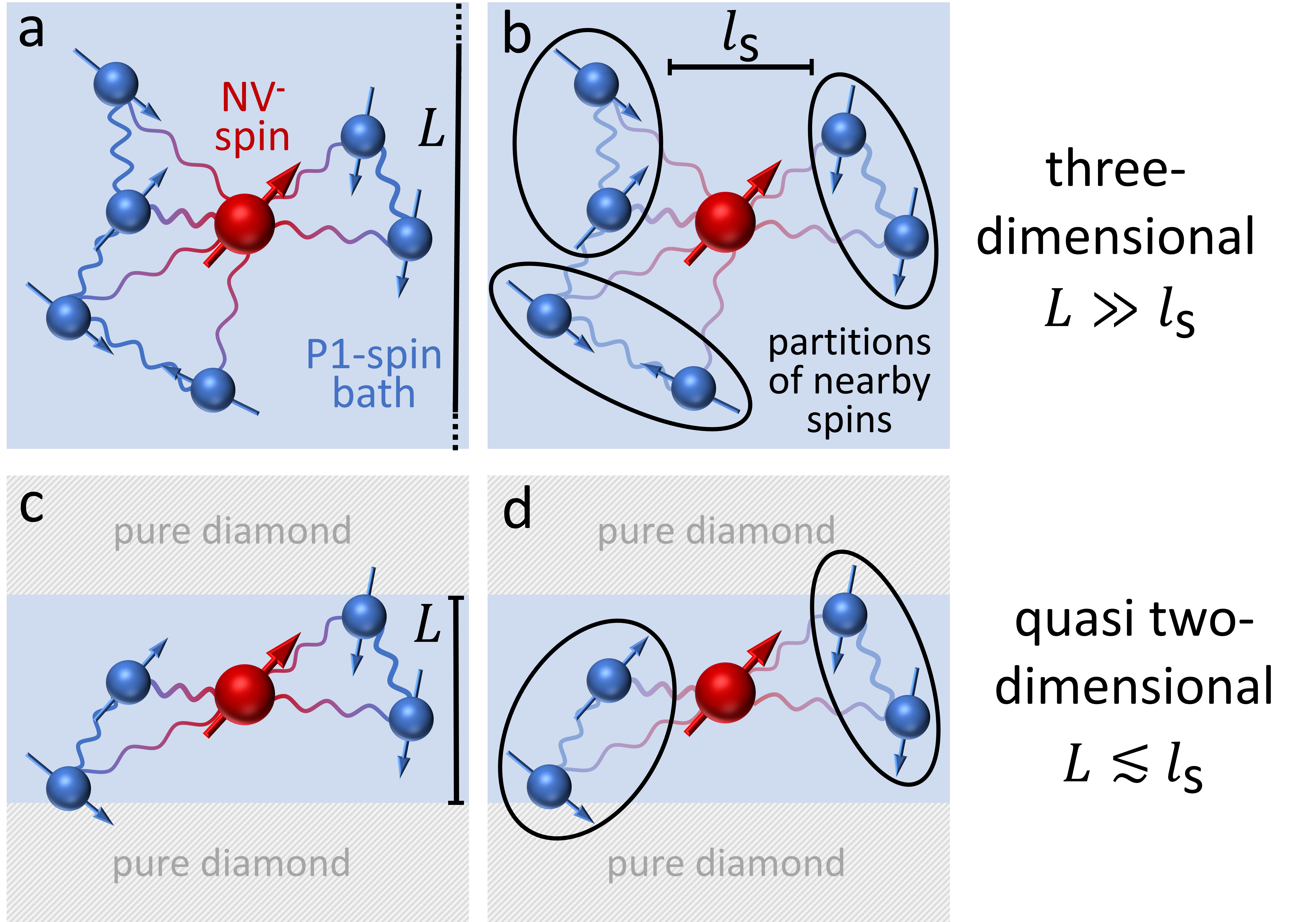
Figure 1: Partitioning the P1-center spin bath of different spatial dimensionality around the NV^--center. Sketch of a three-dimensional (a) and quasi two-dimensional (c) P1-center spin bath, which differ only by the layer thickness $L$. The relation between the layer thickness $L$ and the mean nearest-neighbor spin distance $l_{\text{s}}$ determines the dimensionality of the bath: $L\gg l_{\text{s}}$ for the three-dimensional and $L\lesssim l_{\text{s}}$ for the quasi two-dimensional case. Wavy lines indicate the interaction between the spins. For the novel pCCE method, we first partition the bath into local strongly-interacting indivisible partitions. As an example, two-spin partitions are indicated by the ovals in parts (b) and (d). Then, the conventional CCE method is applied to the partitions. Only the electron spin of the P1-centers is indicated in the figure, nuclear spins are omitted.

For the nitrogen-vacancy (NV^-) center in diamond [25], which offers immense potential for quantum technologies [26, 27, 28, 29, 30, 31, 32, 33, 34, 35, 36, 37], the spin-coherence decay is mainly governed by the interaction with spins of single-substitutional nitrogen defects (called $N_{s}^{0}$ or P1-centers) [10] and the ¹³C nuclear spins [38]. The P1-centers, each comprising an electron spin and a nuclear spin, usually dominate the spin-coherence decay of NV^--centers even at comparatively low concentrations of about 1 ppm due to the large electron-spin gyromagnetic ratio. To suppress the interaction with P1-centers, the material properties of diamond samples can be enhanced [39], for example, by using delta-doping diamond-growth techniques [40, 41, 42] which allow for a precise depth placement of defects with layer thicknesses in the nanometer range. In such thin layers, the P1-center spin bath is typically quasi two-dimensional, leading to longer Hahn-echo $T_{2}$ times [43, 44, 23]. The theoretical analysis of such quasi two-dimensional strongly-coupled baths is particularly difficult due to large fluctuations of dipolar interaction coefficients [45, 46, 47].

In this letter, the results are twofold: First, in the effort to improve diamond samples for quantum-technology devices, we numerically simulate the spin-coherence decay of NV^--spin ensembles in strongly-coupled P1-center spin baths in diamond layers of different thickness and P1-center concentration, thereby identifying parameters for extended spin-coherence time. Second, to overcome difficulties of available methods when applied to strongly-coupled baths, we introduce a novel numerical method used in the above calculations, which is based on the cluster-correlation expansion (CCE) applied to local strongly-interacting partitions of the bath; we name this method partition-CCE (pCCE), cf. Fig. 1.

We calculate the spin-coherence times $T_{2}$ in quasi two-dimensional diamond layers and show that they exceed those in bulk diamond. Our results also indicate two scalings of the $T_{2}$ time with the P1-center concentration $\rho_{\text{P1}}$ due to different spatial dimensionalities of the spin bath: $T_{2}\cong(\rho_{\text{P1}})^{-1}$ for bulk diamond and $T_{2}\cong(\rho_{\text{P1}})^{-3/2}$ for quasi two-dimensional layers depending on the layer thickness $L$. For quasi two-dimensional layers, the mean nearest-neighbor spin distance $l_{\text{s}}$ satisfies $L\lesssim l_{\text{s}}$. Moreover, we show that the stretched-exponential parameter $p$ for the short-time spin-coherence decay is governed by the hyperfine interaction of the P1-centers, which strongly modifies the bath-spin dynamics (see, for example, Ref. [10, 48]). Only when considering P1-centers without the nitrogen nuclear spins in our numerical simulations, the values for $p$ are consistent with predictions from bath-dynamics models based on the Ornstein-Uhlenbeck process [23]. These results constrain random-noise models for the description of P1-center spin baths [49] and offer possibilities for improving the diamond samples by optimized layer thickness and sample growth.

To simulate central-spin dynamics in strongly-coupled baths of different dimensionality, our novel method divides the bath into local strongly-interacting subsystems (which we refer to as partitions in the following) and applies the CCE method [16] to the partitions instead of individual spins. The strongly-interacting partitions are treated as indivisible units. In this way, the method takes into account important higher-order spin correlations leading to improved accuracy of results, broader range of applicability and enhanced convergence properties.

We consider ensembles of NV^--center electron spins (we omit the minus sign in the following) in isotopically purified ¹²C diamond layers with a sparse disordered P1-center spin bath of concentration $\rho_{\text{P1}}$. A strong magnetic field parallel to the NV-axis defines the $z$-axis. In the rotating reference frame, the P1-center electron spins interact via the secular part of the dipolar Hamiltonian [1, 2]

$${\cal H}_{\text{P1}}=\sum_{i>j\geq 1}J_{ij}\left(I_{iz}I_{jz}-\frac{1}{4}[I_{i}^{+}I_{j}^{-}+I_{i}^{-}I_{j}^{+}]\right),$$ (1)

where $I_{jz}$ is the $z$-projection operator for the $j$-th P1-center electron spin, $I_{j}^{+}$ ($I_{j}^{-}$) is the corresponding spin raising (lowering) operator and $J_{ij}\cong 1/r_{ij}^{3}$ is the dipolar coupling constant with $r_{ij}$ being the distance between spins $i$ and $j$. For each P1-center, the hyperfine interaction with the nitrogen nuclear spin reads ${\cal H}_{\text{hf},j}=A_{j}I_{jz}S_{jz}$, where $S_{jz}$ is the spin-1 $z$-projection operator of the nuclear spin and $A_{j}$ is the hyperfine interaction constant, which depends on the Jahn-Teller-axis alignment [10, 48]. An energy mismatch generally suppresses the flip-flop transitions between the NV- and P1-center electron spins such that the corresponding interaction Hamiltonian reads [1, 2] ${\cal H}_{\text{int}}=\sum_{j}J_{0j}I_{0z}I_{jz}$, where the index 0 corresponds to the NV spin. We quantify the spin coherence of the NV spin by $\langle M_{x}(2\tau)\rangle\equiv\langle I_{0x}(2\tau)\rangle/\langle I_{0x}(0)\rangle$, where $\langle I_{0x}(2\tau)\rangle$ is the $x$-magnetization of the NV spin after a Hahn-echo sequence [50]. For a more detailed description of the system, see supplemental material [51].

The interaction with the P1-center spin bath described by ${\cal H}_{\text{int}}$ leads to a time-dependent magnetic field for the NV spin $B^{\text{P1}}_{z}(t)\cong\sum_{j}J_{0j}\langle I_{jz}(t)\rangle$, where $\langle I_{jz}(t)\rangle$ is the expectation value of $I_{jz}$. The characteristics of $B^{\text{P1}}_{z}(t)$ are governed by the dynamics of the P1-center bath, which is in turn dominated by the flip-flop transitions described in Eq. (1). Generally, the Hahn-echo sequence cannot fully refocus an initial polarization of the NV spin for such time-dependent magnetic fields. Instead, the NV spin dephases in the $(x,y)$-plane corresponding to the decay of the spin coherence $\langle M_{x}(2\tau)\rangle$.

The main idea of the CCE method is to approximate the collective spin-bath dynamics by the dynamics of all possible small subsystems (clusters) of size (number of spins) $n$ up to an order $n\leq N$ (CCE$N$). The effects of the individual cluster dynamics on the central spin are then assembled to form the joint effect (for a detailed definition, see supplemental material [51]). When calculating the quantum spin dynamics in a chosen cluster, all other bath spins are included on the mean-field level, i.e., they are static [52, 53, 54], and the final result is to be averaged over the mean-field spin configurations. For practical calculations of the spin coherence of an NV electron spin in the weakly-coupled bath of nuclear spins, CCE2 is often used, which includes the dynamics of single spins and spin pairs in the bath; see, for example, Refs. [43, 55].

In the strongly-coupled P1-center spin bath, the dynamics in the bath takes place on the same timescale as the spin-coherence decay of the NV spin. Hence, correlated bath dynamics of higher order than for the nuclear-spin bath must usually be taken into account. Therefore, higher order CCE$N$ ($N>2$) need to be applied, which, however, often show unphysical behaviour for strongly-coupled spin baths [52, 53], when, for example, $|\langle M_{x}(2\tau)\rangle|>1$ for an initially fully polarized NV spin. This can occur, for example, when clusters in the CCE method include only a part of a strongly-interacting spin group. In principle, this issue can be corrected for by further increasing $N$ but, in practice, this in turn introduces even more clusters with unphysical behaviour.

The main idea of the pCCE method is to divide the disordered spin bath into strongly-interacting local subsystems (partitions) and to apply the conventional CCE method to the partitions instead of individual spins, cf. Fig. 1. The partitions are chosen such that the interaction inside the partitions is maximized. These strongly-interacting partitions in the bath act as indivisible units when applying the CCE method [51], thereby facilitate capturing the correct spin dynamics. We choose for simplicity partitions with an equal number of spins $K$ (partition size) and adopt the notation pCCE($N,K$), when applying CCE$N$ after partitioning the bath into $K$-spin partitions. Using pCCE($N,K$), the clusters are formed by combining up to $N$ partitions. In pCCE(2,2), for example, CCE2 is applied to partitions of strongly-interacting spin pairs as illustrated in Fig. 1. In particular, pCCE($N$,1) is equivalent to CCE$N$.

The pCCE method offers several advantages by construction. At sufficiently large $K$, each strongly-interacting spin group is included in a single partition, thereby capturing important higher-order spin correlations. Moreover, in contrast to the CCE method, the number of samples for the mean-field average decreases with increasing $K$, cf. Fig. 2 (for details about the mean-field average, see supplemental material [51]). Further, pCCE($N,K+1$) is not based on results of pCCE($N,K$) because the partitioning of the bath significantly changes. Therefore, to increase the accuracy of results at larger $K$, the pCCE method does not rely on correcting inaccuracies of results at smaller $K$. Hence, the order $K$ is effectively unrestricted.

To demonstrate the performance of the pCCE method, $\langle M_{x}(2\tau)\rangle$ for the NV spin interacting with a small disordered quasi two-dimensional bath of 20 electron spins-1/2 is shown for different values of $K$ in Fig. 2. With increasing partition size $K$, the pCCE results converge towards the exact solution and become almost indistinguishable from the exact solution at $K=4$. This demonstrates the power of the pCCE method to capture the relevant dynamics and even approach the exact solution with a relatively low partition size $K$.

Extensive tests of the pCCE($2,K$) performance for large spin baths show that $K=4$ is required for the method to be sufficiently accurate for all systems considered. The most demanding systems requiring $K=4$ are quasi two-dimensional layers of P1-centers without the hyperfine interaction, i.e., electron spins-1/2, which implies that the correlated spin dynamics extends over local spin subsystems of at most $NK=8$ spins on the relevant timescales, thereby establishing an indirect measure of correlations in the bath. For P1-center spin baths (inlcuding the hyperfine interaction), pCCE converges already at $K=1$ corresponding to CCE2, which we attribute to the complex substructure in the bath suppressing flip-flop transition as discussed below (for convergence tests, see supplemental material [51]). We use $K=4$ for all systems in the following. In principle, the order $N$ could also be increased for pCCE but, for our calculations, this was not necessary. For the results described below, we perform disorder average over 100 randomly chosen spin distributions and average over 20 mean-field spin configurations for each system.

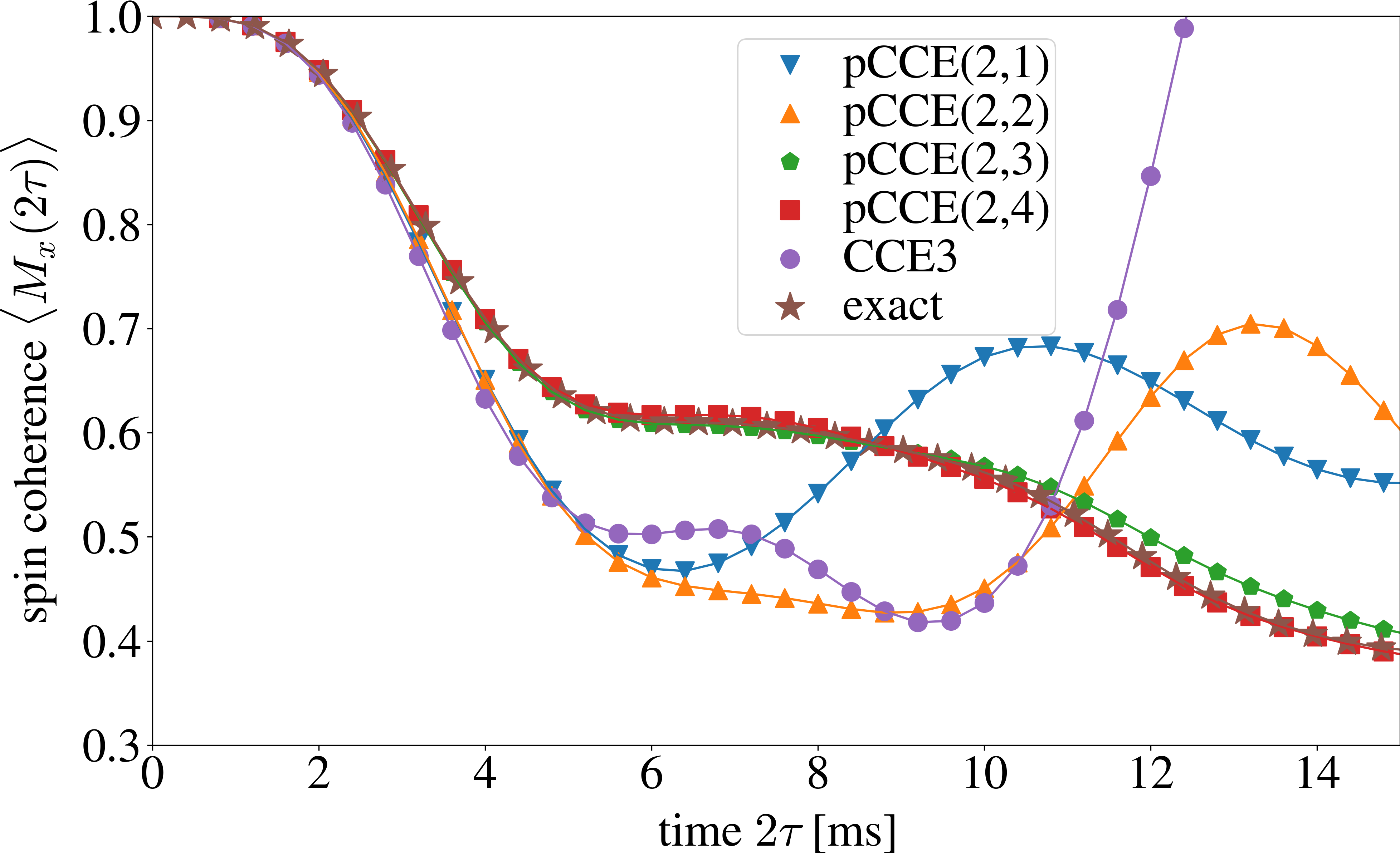
Figure 2: Performance of the pCCE method and comparison to CCE. The time evolution of the spin coherence $\langle M_{x}(2\tau)\rangle$ of the NV electron spin in a quasi two-dimensional bath of 20 randomly distributed electron spins-1/2 is shown. Increasing the partition size $K$, the pCCE results converge towards the exact solution. Exact results were obtained using the Suzuki-Trotter expansion [56]. Lines connect points to guide the eye. The number of samples for the mean-field average decreases for pCCE with larger $K$, whereas it increases for CCE with larger $N$. For example, pCCE(2,4) converged after averaging over 10 mean-field configurations but CCE3 results shown here have not converged after averaging over 1000 mean-field configurations. For details about the mean-field averaging, see supplemental material [51].

Let us now discuss pCCE results for the spin-coherence $\langle M_{x}(2\tau)\rangle$ decay of NV spins interacting with the P1-center spin bath. On short timescales [51], $\langle M_{x}(2\tau)\rangle$ is generally expected to follow a stretched-exponential function [4]

$$\langle M_{x}(2\tau)\rangle\approx\exp\left[-\left(\frac{2\tau}{T_{2}}\right)^{p}\right].$$ (2)

For a well-defined stretched-exponential parameter $p$, the function $-\ln(\langle M_{x}(2\tau)\rangle)$, when plotted on a double-logarithmic scale, is expected to exhibit a linear behaviour with slope $p$. At short times, the results obtained indeed indicate a linear behavior, see Fig. 3. Fitting the function in Eq. (2) to the numerical results in this regime, we obtain $p$ and $T_{2}$ for different values of the diamond-layer thickness $L$ and the P1-center concentration $\rho_{\text{P1}}$, see Fig. 4. There are two different scalings of the $T_{2}$ time as a function of $\rho_{\text{P1}}$, which we attribute to different spatial dimensionalities of the spin bath: $T_{2}\cong(\rho_{\text{P1}})^{-1}$ for bulk diamond at larger layer thicknesses (e.g. the slope is -1.02 for $L=240$ nm) and $T_{2}\cong(\rho_{\text{P1}})^{-3/2}$ for quasi two-dimensional layers (e.g. the slope is -1.46 for $L=30$ nm) [47]. The quasi two-dimensional nature of the $L=30$ nm layer at the concentrations $\rho_{\text{P1}}$ considered is confirmed by relating $L$ to the mean nearest-neighbor spin distance $l_{\text{s}}=l_{\text{s}}(\rho_{\text{P1}})$: at $L=30$ nm, $L/l_{\text{s}}$ varies approximately between 1.5 and 3 depending on $\rho_{\text{P1}}$ and, for $L=240$ nm, $L/l_{\text{s}}>10$. For intermediate $L$, both regimes can be observed in Fig. 4: at larger $\rho_{\text{P1}}$, the spin bath tends to the three-dimensional case and, for smaller $\rho_{\text{P1}}$, to the two-dimensional case. These novel results highlight the broad range of applicability of the pCCE method and open new avenues to optimized material properties.

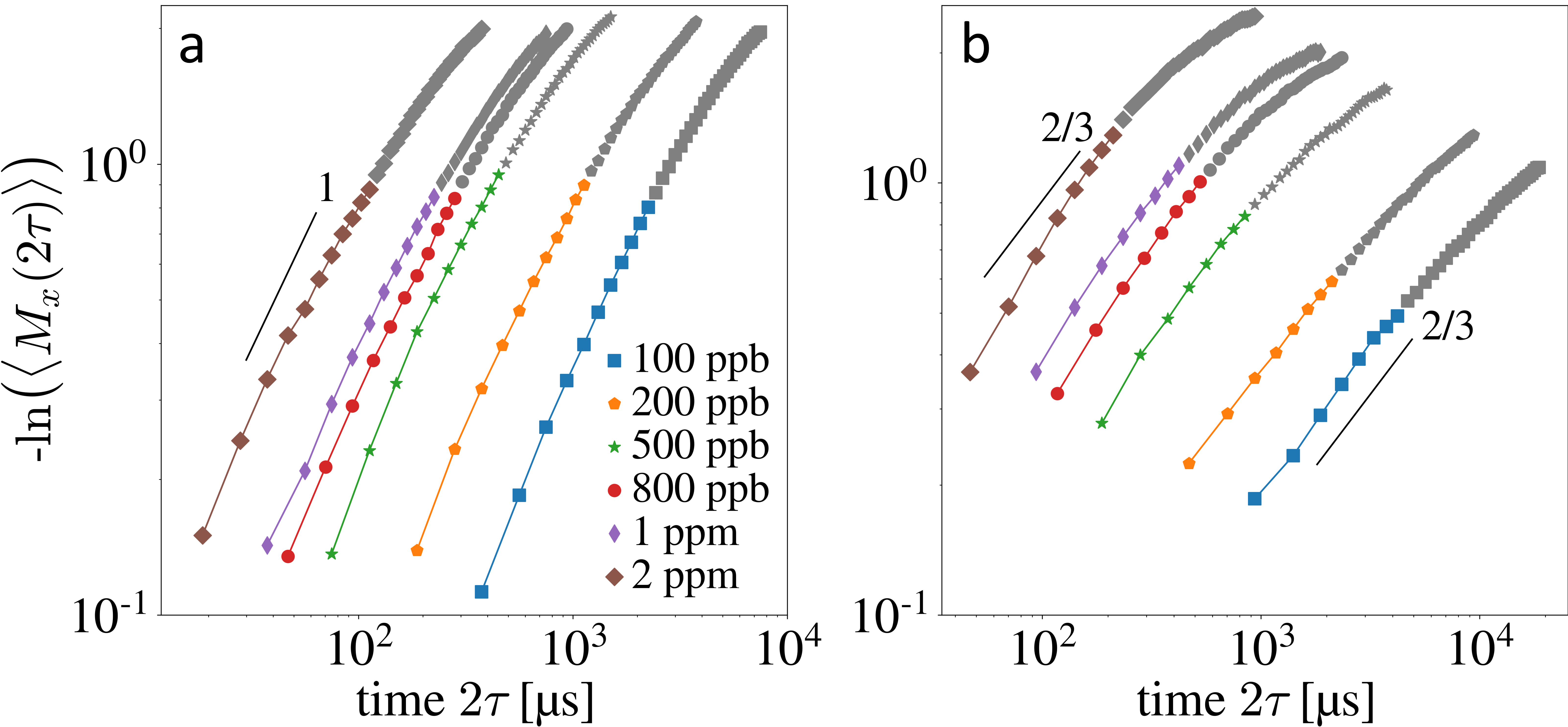
Figure 3: Evidence for stretched-exponential behavior of the spin coherence $\langle M_{x}(2\tau)\rangle$ on short timescales. The function $-\ln(\langle M_{x}(2\tau)\rangle)$ plotted on a double-logarithmic scale at layer thickness $L=240$ nm (a) and $L=60$ nm (b) for various P1-center concentrations $\rho_{\text{P1}}$ as indicated in the legend. The slope of the initial linear behavior corresponds to the stretched-exponential parameter $p$. In part (a), the layer thickness $L=240$ nm corresponds to bulk diamond for all $\rho_{\text{P1}}$ considered ($p\approx 1$). In part (b), the slope is changing corresponding to a transition from quasi two- ($p\approx 2/3$) towards three-dimensional bath when increasing $\rho_{\text{P1}}$ ($p>2/3$). The values used for fitting are indicated by the lines connecting the colored points. For $\langle M_{x}(2\tau)\rangle$, this range approximately corresponds to the decay from 0.9 to 0.5.

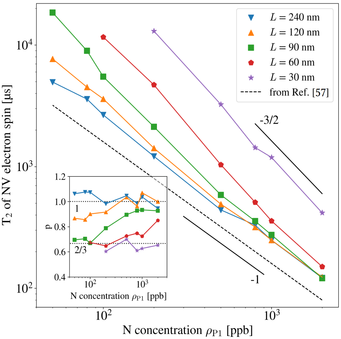
Figure 4: Coherence time $T_{2}$ and the stretch-exponential parameter $p$ signalling the spatial bath dimensionality. The $T_{2}$ time of the NV-center electron spin in a P1-center spin bath is shown for various P1-center concentrations $\rho_{\text{P1}}$ and layer thicknesses $L$ as indicated in the legend. Different scalings $T_{2}\cong(\rho_{\text{P1}})^{-1}$ and $T_{2}\cong(\rho_{\text{P1}})^{-3/2}$ are indicated by short black lines. The dashed black line is a fit to experimental results from Ref. [57]. Inset: The corresponding stretched-exponential parameters $p$ with two distinguished values $p\approx 1$ for bulk diamond and $p\approx 2/3$ for quasi two dimensional layers. At intermediate $L$, we observe a smooth transition from the quasi-two-dimensional case ($p\approx 2/3$) to the bulk diamond ($p\approx 1$) when increasing $\rho_{\text{P1}}$. Lines connect points to guide the eye. Fluctuations are presumably due to a finite number of samples for the averaging and uncertainties when identifying the time window for fitting.

Table 1: Evidence for the dependence of the stretched-exponential parameters $p$ on the hyperfine interaction in the P1-center bath. For the quasi two-dimensional and the three-dimensional case, $p$ is calculated including (P1-center) and excluding (no hyperf.) the hyperfine interaction for various spin concentrations $\rho$. We estimate the error of each of the values shown to be at least $\pm 0.1$ [51].

	$\rho$	2 ppm	1 ppm	0.1 ppm
two-dim.	P1-center	0.65	0.63	0.67
($L\leq$60 nm)	no hyperf.	0.95	1.09	1.05
three-dim.	P1-center	0.95	1.04	1.08
($L$=240 nm)	no hyperf.	1.62	1.55	1.51

The $T_{2}$ times obtained are in agreement with experimentally measured values. For example, we obtain at $\rho_{\text{P1}}=2$ ppm for bulk diamond ($L=240$ nm) $T_{2}\approx 122\,\mu$s and the experimentally measured value is $T^{\text{exp}}_{2}\approx 80\,\mu$s [57]. In general, the calculated $T_{2}$ times are considered upper bounds because of other potential sources of dephasing in diamond samples, which is presumably one of the reasons for the difference between the above values.

The corresponding values for $p$ are shown in the inset of Fig. 4. We obtain $p=1.03\pm 0.05$ for bulk diamond ($L=240$ nm) and $p=0.64\pm 0.05$ for quasi two-dimensional layers ($L=30$ nm) . For intermediate diamond layer thicknesses $L$, we obtain a smooth transition between these two cases as we vary $\rho_{\text{P1}}$. Interestingly, if we leave out the nuclear spins of the P1-centers in our simulations, such that each P1-center is an electron spin-1/2, we obtain on average $p=1.56\pm 0.06$ and $p=1.05\pm 0.09$ for the bulk and the quasi two-dimensional case, respectively, see Table 1. These values are consistent with those analytically predicted by bath-dynamics models based on the Ornstein-Uhlenbeck process [23]. We attribute these findings to the complex internal substructure of the P1-center spin bath caused by the hyperfine interaction described by ${\cal H}_{\text{hf},j}=A_{j}I_{jz}{S}_{jz}$, where $A_{j}$ depends on the orientation of the Jahn-Teller axis of the P1-defects ($A_{j}=114$ MHz for the [111]-axis and $A_{j}=86$ MHz otherwise). The energy splittings induced by this interaction are much larger than the dipole-interaction constants at the concentrations $\rho_{\text{P1}}$ considered [51]. Therefore, the P1-center bath is effectively divided into five subgroups depending on the orientation of the nuclear spins and the Jahn-Teller axes. Flip-flop transitions between P1-center electron spins from different subgroups are strongly suppressed (see, for example, Ref. [10, 48]). Effectively, this situation corresponds to a NV spin in presence of five coupled spin baths with different characteristic times [51]. Even if the baths were uncoupled, the sum of Ornstein-Uhlenbeck processes describing the individual baths would typically not correspond to an Ornstein-Uhlenbeck process. We ascribe the dependence of the stretched-exponential parameter on the hyperfine interaction to this complexity in the bath.

To conclude, we investigate the spin-coherence decay of NV^--spins interacting with the strongly-coupled disordered bath of the single-substitutional nitrogen defects in diamond layers. We obtain, for quasi two dimensional diamond layers, $T_{2}$ times which exceed those in bulk diamond, hence allowing to surpass the limit imposed by the defect concentrations in bulk diamond. We show that the stretched-exponential parameter $p$ for the short-time spin-coherence decay is governed by the hyperfine interaction of the P1-centers, which strongly modifies the bath-spin dynamics. Only when considering P1-center spins without the nitrogen nuclear spins in our numerical simulations, the values for $p$ correspond to those from bath-dynamics models based on the Ornstein-Uhlenbeck process. We introduce the novel pCCE method based on the cluster-correlation expansion applied to local strongly-interacting partitions of the bath, which includes important high-order spin correlations leading to better accuracy, applicability to longer timescales and enhanced convergence properties. We expect this method to be applicable far beyond the setting considered here: for example, to NMR systems, i.e., nuclear spins on a lattice, to longer pulse sequences such as the Carr-Purcell-Meiboom-Gill pulse sequence and perhaps even to non-Markovian spin baths.

The authors would like to thank V. V. Dobrovitski and G. A. Starkov for discussions of this work. PS and WH acknowledge funding from the executive-board project “Quantum Computing” - an initial project for the realization of a quantum computer of the Fraunhofer-Gesellschaft (QuaComVor). The source code is published in a GitHub repository [59].

Supplemental material for the manuscript “Extended Spin-Coherence Time in Strongly-Coupled Spin Baths in Quasi Two-Dimensional Layers”

Note: In this supplemental material, we use the same notations as in the main article. Equation numbers, figure numbers and table numbers without an “S” refer to the main article.

I Detailed description of the system

In this section, we discuss the NV-center spin system, the interaction between the NV-center and the P1-center bath, describe details about the P1-center spin bath and, at the end, present the total Hamiltonian.

I.1 NV-center

We consider ensembles of NV-centers in [111]-oriented isotopically purified ¹²C diamond with a sparse disordered P1-center spin bath of concentration $\rho_{\text{P1}}$. Due to relatively long distances between the P1-centers, all defects can be treated as localized spins interacting via dipolar interaction. The diamond sample is placed in a strong magnetic field $B_{z}$ along the $z$-direction, which is also the [111]-direction, such that the three energy levels of the NV electron spin-1 are well separated (the NV-center nuclear spin is neglected, see below). In presence of this magnetic field $B_{z}$, the internal Hamiltonian of the NV electron spin in the laboratory reference frame reads ${\cal H}^{\text{lab}}_{\text{NV}}=DS_{z}^{2}-\gamma B_{z}S_{z}$, where $D$ denotes the zero-field splitting, $S_{z}$ is the z-projection spin-1 operator and $\gamma$ the electron-spin gyromagnetic ratio. The NV spin is initialized in $|\psi(0)\rangle=\frac{1}{\sqrt{2}}(|0\rangle+|-1\rangle)$, where $|0\rangle$ and $|-1\rangle$ are eigenstates of $S_{z}$ with corresponding eigenvalues. The state $|+1\rangle$ remains unoccupied on the timescales considered because the $z$-component of the NV spin is conserved by ${\cal H}^{\text{lab}}_{\text{NV}}$ and the interaction Hamiltonian with the P1-center spin bath $\cal H_{\text{int}}$ (see below). The NV spin can thus be effectively treated as a spin-1/2 with the adapted $z$-projection operator

$$I_{z}=\begin{pmatrix}0&0\\ 0&-1\end{pmatrix}.$$ (S1)

In the reference frame rotating with the Larmor frequency $\gamma B_{z}$, the NV-electron-spin Hamiltonian reads ${\cal H}_{\text{NV}}=-DI_{0z}$, where the index 0 refers to the NV electron spin.

We study the spin coherence of the NV spin, which we quantify by

$$\langle M_{x}(2\tau)\rangle\equiv\frac{\langle I_{0x}(2\tau)\rangle}{\langle I_{0x}(0)\rangle},$$ (S2)

where $\langle I_{0x}(2\tau)\rangle$ is the $x$-magnetization of the NV spin after a Hahn-echo sequence. A Hahn-echo sequence consists of the Hamiltonian time evolution of the system with time $\tau$, followed by a $\pi$-pulse along the $x$-axis for the NV spin and another Hamiltonian time evolution with time $\tau$ [50]. For the above initial state $|\psi(0)\rangle$, we obtain $\langle I_{0x}(0)\rangle=1/2$, such that $\langle M_{x}(2\tau)\rangle=2\langle I_{0x}(2\tau)\rangle$. Since the state $|\psi(0)\rangle$ corresponds to a fully polarized state in the Hilbert subspace described above, $\langle M_{x}(2\tau)\rangle\in[-1,1]$. Hence, we refer to any numerical result $|\langle M_{x}(2\tau)\rangle|>1$ as unphysical.

The ¹⁴N nuclear spin of the NV center can be assumed static on the timescales considered. The dominating interaction term in the strong magnetic field $B_{z}$ is of the form $I_{z}\tilde{S}_{z}$ [1], where $\tilde{S}_{z}$ is the $z$-projection operator of the nuclear spin. Such interaction would create an effective static magnetic field along the $z$-direction for the NV electron spin. Therefore, the effect of the NV nuclear spin on the NV electron spin is cancelled in the Hahn-echo sequence. Hence, we do not include the ¹⁴N nuclear spin in our numerical simulations.

I.2 Interaction between the NV spin and the P1-center spin bath

The central spin and the P1-center bath spins interact by dipolar coupling with coupling constants $J_{ij}=\mu_{0}\gamma^{2}(1-3\cos^{2}(\theta_{ij}))/4\pi|\vec{r}_{ij}|^{3}$, where $\theta_{ij}$ is the angle between the vector $\vec{r}_{ij}$ connecting the spins and the axis of the applied magnetic field, which defines the $z$-axis. The magnetic field is usually chosen such that the NV electron spin and the P1-center electron spins are not in resonance. Therefore, the flip-flop terms in the dipolar Hamiltonian are suppressed and the only secular part remaining in the rotating reference frame is

$${\cal H}_{\text{int}}=\sum_{j\geq 1}J_{0j}I_{0z}I_{jz},$$ (S3)

where the index 0 corresponds to the NV electron spin and $j\geq 1$ to P1-center electron spins.

The P1-center spins are assumed to be in the infinite-temperature limit, when each P1-center spin is described by a fully mixed density matrix

$$\rho=\begin{pmatrix}1/2&0\\ 0&1/2\end{pmatrix}.$$ (S4)

I.3 P1-center spin bath

A P1-center consists of an electron spin-1/2 and a ¹⁴N nuclear spin-1. Between the P1-centers, the interaction is dominated by the dipolar interaction between the respective electron spins. The corresponding Hamiltonian ${\cal H}_{\text{P1}}$ is given in Eq. (1) of the main text.

For each P1-center, the strong hyperfine interaction in the rotating reference frame is of the form

$${\cal H}_{\text{hf},j}=A_{j}I_{jz}S_{jz},$$ (S5)

where $A_{j}$ is the hyperfine interaction constant and $S_{jz}$ is the z-projection operator for the nuclear spin-1 of $j$-th P1-center [10, 48]. The hyperfine interaction constant $A_{j}$ depends on the orientation of the Jahn-Teller (JT) axis of the P1-center: for the [111]-axis (corresponding to the $z$-axis here), $A_{j}=114$ MHz, and $A_{j}=86$ MHz for the other three possible axis alignments. For the P1-center concentrations $\rho_{\text{P1}}$ considered here, the energy splittings induced by the hyperfine interaction are much larger than the dipole-interaction constants (see below) and, therefore, two P1-center electron spins can flip-flop only if the orientation of the corresponding nuclear spins and the JT axes is the same for the two P1-centers. Hence, the P1-center bath is effectively divided into five spin subgroups depending on the orientation of both, the JT axes and the nitrogen nuclear spins. Any P1-center remains in the same subgroup on the timescales of our simulations, because the nuclear spin dynamics as well as the JT reorientation have significantly longer characteristic timescales [60]. This complex structure of the P1-center bath implies that the majority of nearest neighbors of any P1-center spin is likely to belong to a different subgroup. These nearest neighbors create strong disordered local fields for the P1-center spin by means of the first Hamiltonian term in Eq. (1) but do not flip-flop with it.

The above P1-center bath subgroups are not equally sized. In order to understand this, let us first consider the individual configurations for the nuclear-spin polarization and the JT-axis alignment. The different $m_{s}$ states for the nuclear spins are $|+1\rangle$, $|-1\rangle$ and $|0\rangle$. For the first two states, there are the two inequivalent JT axes alignments: JT along [111] and JT not along [111]; we denote the latter case by $\overline{[111]}$ (it comprises the three equivalent alignments [$\overline{1}$11], [1$\overline{1}$1] and [11$\overline{1}$]). For the state $|0\rangle$, the hyperfine interaction term vanishes, thus the JT-axis alignment remains unimportant. For an even distribution among the nuclear-spin states (infinite temperature) and the JT alignments [60], the probability $P$ for the different configurations is as follows: for $|+1\rangle$ and [111]: P=1/12, for $|-1\rangle$ and [111]: P=1/12, for $|+1\rangle$ and $\overline{[111]}$: P=3/12, for $|-1\rangle$ and $\overline{[111]}$ P=3/12, for $|0\rangle$: P=4/12 (in this case, the JT-axis alignment is unimportant). It is also noteworthy that the different sizes of the P1-center bath subgroups lead to different effective spin concentrations in the individual subgroups and, hence, to different characteristic times for the dynamics in these subgroups.

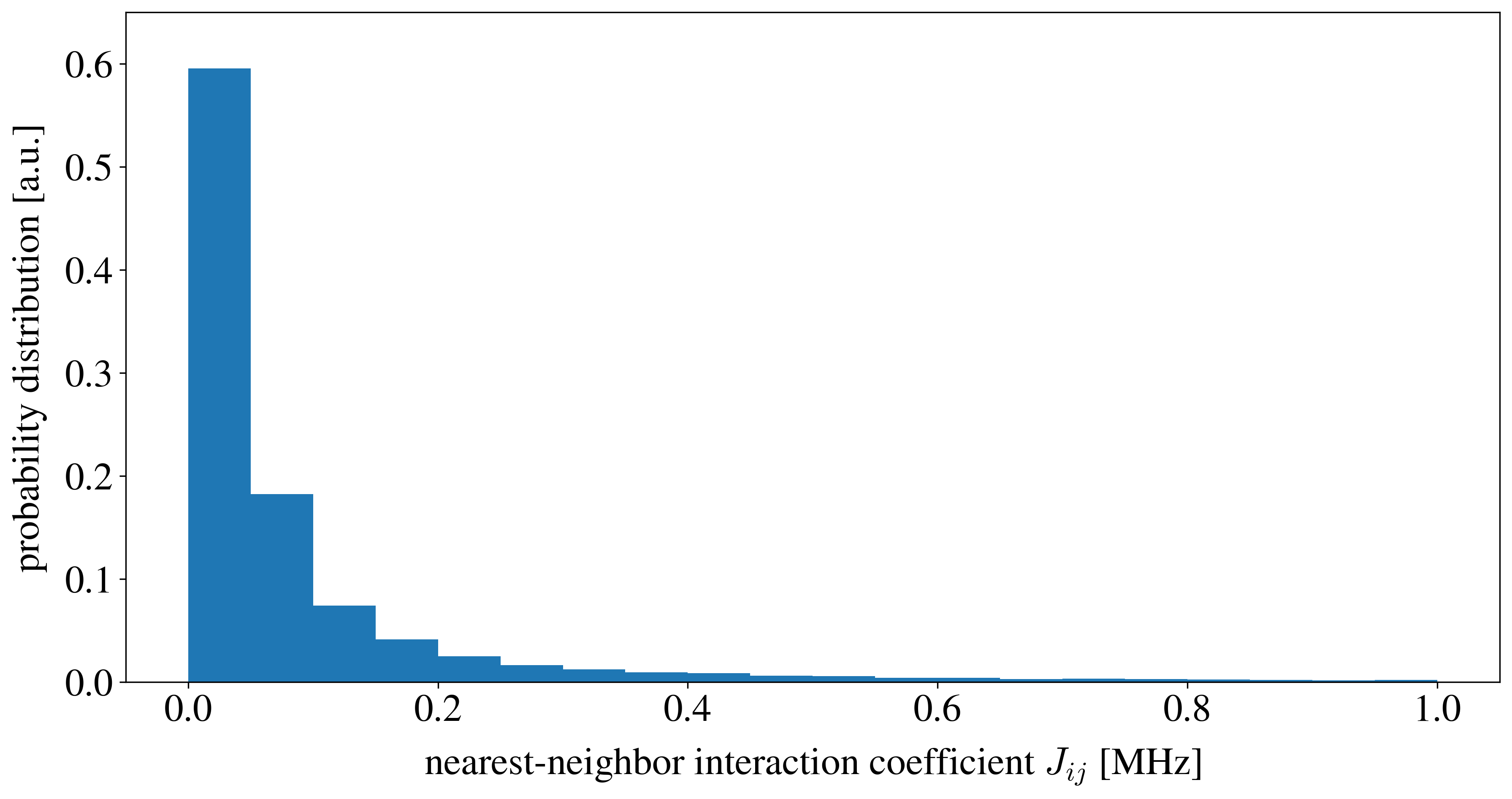
Figure S1: Histogram of nearest-neighbor interaction constants $J_{ij}$ in a three-dimensional diamond layer at the highest concentration $\rho_{\text{P1}}=2$ ppm considered in this letter. The overwhelming majority of nearest-neighbor interactions constants is well below the smallest hyperfine energy splitting of 28 MHz induced by different JT-orientations. At lower concentrations $\rho_{\text{P1}}$, the interaction constants $J_{ij}$ become even smaller. These results confirm the assumption, that the P1-center bath is effectively split into subgroups. For details, see the text.

The validity of the assumption that spins from different subgroups do not flip-flop with each other is dependent on the P1-center concentration $\rho_{\text{P1}}$ because the dipolar interaction coefficients increase with larger concentration $\rho_{\text{P1}}$. The highest P1-defect concentration we consider in this work is $\rho_{\text{P1}}=2$ ppm. We calculate the nearest-neighbor interaction constants for each spin in 100 randomly chosen systems at this concentration $\rho_{\text{P1}}=2$ ppm; the resulting histogram is shown in Fig. S1. The overwhelming majority of nearest-neighbor interactions is well below the smallest hyperfine energy splitting of 28 MHz induced by different JT-orientations. At lower concentrations $\rho_{\text{P1}}$, the interaction constants $J_{ij}$ shift to even lower values. This corroborates our assumption, that spins from different subgroups do not flip-flop with each other.

I.4 Total Hamiltonian

Let us now put together all terms discussed above. The total Hamiltonian ${\cal H}_{\text{tot}}$ considered reads

$${\cal H}_{\text{tot}}={\cal H}_{\text{NV}}+\cal H_{\text{int}}+\cal H_{\text{P1}}+{\cal H}_{\text{hf}},$$ (S6)

where ${\cal H}_{\text{NV}}$ describes the NV-center, $\cal H_{\text{int}}$ describes the interaction between the NV center and the P1-center bath, $\cal H_{\text{P1}}$ describes the interaction between the P1-centers and ${\cal H}_{\text{hf}}$ describes the hyperfine interaction for each P1-center. Substituting the individual terms in the expression above, the total Hamiltonian ${\cal H}_{\text{tot}}$ in the rotating reference frame reads

$${\cal H}_{\text{tot}}=-DI_{0z}+\sum_{j\geq 1}J_{0j}I_{0z}I_{jz}+\sum_{i>j\geq 1}J_{ij}\left(I_{iz}I_{jz}-\frac{1}{4}[I_{i}^{+}I_{j}^{-}+I_{i}^{-}I_{j}^{+}]\right)+\sum_{j\geq 1}A_{j}I_{jz}S_{jz}.$$ (S7)

For the dynamics in a Hahn-echo sequence, the effect of the first term ${\cal H}_{\text{NV}}$ is cancelled and, hence, this term can be left out.

The hyperfine interaction ${\cal H}_{\text{hf}}$ (last term in Eq. (S7)) describes effectively an additional constant magnetic field along the $z$-axis, since all $S_{jz}$ are conserved on the timescales considered here. These terms can be omitted by considering a rotating reference frame with rotation frequency dependent on the P1-center bath subgroups discussed above. The flip-flop Hamiltonian terms for two P1-center electron spins from different subgroups acquire a fast oscillating term in this rotating reference frame and, hence, these flip-flop terms are suppressed and can be left out. In our numerical simulations, we consider this rotating reference frame.

II Cluster-correlation expansion (CCE) method

The cluster-correlation expansion (CCE) method [16] allows to approximate the spin-coherence evolution $\langle M_{x}(2\tau)\rangle$ of a central spin in a large bath of spins by considering the contributions of all possible clusters in the bath up to a given size $n\leq N$ (CCE$N$). For an $n$-spin cluster ${\cal C}_{ni}$, where $i$ counts all $n$-spin clusters, $\langle M_{x}(2\tau)\rangle_{ni}$ is obtained by calculating the quantum dynamics only of spins in the cluster ${\cal C}_{ni}$, while all other bath spins are included on the mean-field level, i.e., they are static [53, 54]. The genuine $n$-spin contribution of the cluster ${\cal C}_{ni}$ is defined recursively by

$$\widetilde{\cal L}_{ni}\equiv\frac{\langle M_{x}(2\tau)\rangle_{ni}}{\prod_{{\cal B}\subset{\cal C}_{ni}}\widetilde{\cal L}_{\cal B}},$$ (S8)

where ${\cal B}$ runs over all possible subclusters of ${\cal C}_{ni}$. The total genuine $n$-spin contribution of the bath is $\widetilde{\cal L}_{n}\equiv\prod_{i}\widetilde{\cal L}_{ni}$, where all possible $n$-spin clusters are considered. Finally, for CCE$N$, the spin coherence is approximated by

$$\langle M_{x}(2\tau)\rangle\approx\langle\langle\widetilde{\cal L}_{0}\widetilde{\cal L}_{1}\widetilde{\cal L}_{2}\cdots\widetilde{\cal L}_{N}\rangle\rangle,$$ (S9)

where $\langle\langle...\rangle\rangle$ denotes the average over mean-field spin configurations. For this average, a mean-field configuration is randomly chosen for each P1-center electron spin, i.e., either up or down along the $z$-direction. In the calculations of $\langle M_{x}(2\tau)\rangle_{ni}$, these mean-field spin configurations are chosen for all spins outside the cluster ${\cal C}_{ni}$. The average over mean-field configurations is performed for the total factor on the right-hand-side in Eq. (S9). We refer to this mean-field average as the normal average in the following.

III Internal mean-field averaging

In this section, we discuss another type of mean-field bath-spin averaging often used for the suppression of unphysical CCE results (see, for example, Refs. [52, 53, 54]).

Internal mean-field averging is defined as follows: each term $\widetilde{\cal L}_{ni}$ is averaged over mean-field spin configurations separately before the individual factors are put together as shown in Eqs. (S8) and (S9). When using the internal averaging, correlations between the individual factors on the right-hand-side of Eqs. (S8) and (S9) are neglected. However, for disordered spin baths, these correlations seems to be negligible in practical calculations, cf. Fig. (2).

The internal averaging is particularly useful in CCE calculations with many unphysical terms, i.e., many clusters with $\langle M_{x}(2\tau)\rangle_{ni}>1$. When using internal averaging, the numerator and each term in the denominator in Eq. (S8) are averaged separately and this leads to the suppression of unphysical terms. The two kinds of averaging (normal and internal) can be combined in the following way. When obtaining the result for $\langle M_{x}(2\tau)\rangle$ in Eq. (S9) with internal averaging, this calculation can be repeated many times, thereby averaging over results for $\langle M_{x}(2\tau)\rangle$. We use both types of mean-field averaging in this letter as indicated below.

For Fig. 2 of the main text, the number of samples for normal and internal averaging is as follows: pCCE(2,1) 50 normal without internal, pCCE(2,2) 50 normal with 50 internal, pCCE(2,3) 50 normal with 20 internal, pCCE(2,4) 10 normal without internal, CCE3 1000 internal. For the calculation of the $T_{2}$ time and the stretched-exponential parameter $p$ in P1-center baths (with and without the hyperfine interaction), we use pCCE(2,4) with 20 samples for internal averaging. In general, for larger partition size $K$, the number of samples for the mean-field averaging decreases for pCCE, while it increases for CCE for larger $N$. This illustrates one of the advantages of the pCCE method. The reason for the decreasing number of samples for the mean-field averaging for the pCCE method is that the average over spins in the clusters is already included by the quantum-mechanical average and that the clusters consist of local partitions.

When increasing the partition size beyond $K=4$, we observed that, for $K=5$ and $K=6$, the number of samples for the mean-field average further decreases, so we expect that, for sufficiently large $K$, neither internal nor normal mean-field average is required. Using exact methods for the time propagation, pCCE(2,10) or even larger partition sizes are feasible.

IV Comparison of results of the pCCE method and exact simulations for small systems

To study the convergence behaviour of the pCCE method, we calculate the spin coherence $\langle M_{x}(2\tau)\rangle$ of NV spins in small baths of 20 electron spins-1/2. Here, we discuss results for three different spatial spin distributions, a two-dimensional spin lattice and two random three-dimensional baths, and compare the numerical pCCE results with results of an exact simulation. The exact simulations were performed using the Suzuki-Trotter method [56].

As the first example, we discuss results for a spin-lattice system with bath spins being placed on a two-dimensional lattice with nearest-neighbor distance of 20 nm. The results obtained with the pCCE method for different partition size $K$ are shown in Fig. S2 (a). Increasing the partition size $K$, the results converge towards the exact solution; an exception is pCCE(2,2) showing unphysical behavior. This behavior is suppressed when using internal mean-field averaging, as illustrated in Fig. S2 (a) by the green curve.

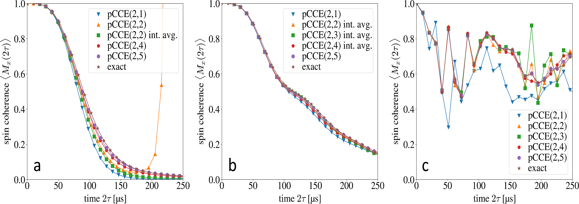
Figure S2: Spin coherence $\langle M_{x}(2\tau)\rangle$ decay of the NV-electron spin in three different small baths of 20 electron spins-1/2: (a) a two-dimensional spin lattice, and (b) - (c) three-dimensional spin baths with random spin distributions at concentration 1 ppm (see text). In all three cases, the pCCE results converge towards the exact results when increasing $K$. To demonstrate the effect of internal mean-field averaging, we also include results with and without internal mean-field average. Results obtained with internal averaging are labeled as “int. avg.”. In (b), already the CCE2 (equivalent to pCCE(2,1)) results show good agreement with exact results, whereas, in (c), there are sizable deviations between CCE2 and the exact solution.

The deviation of CCE2 results from the exact solution depends on the particular spin system considered [53]. Sparse spin systems can cause vastly different decays depending on the spatial spin arrangement. To illustrate this, we chose two different three-dimensional systems and show results for these systems in Fig. S2 part (b) and (c). Both spin systems were obtained by placing the bath electron spins on a diamond lattice at a concentration of 1 ppm and then selecting the 20 closest spins to the central NV center. For the first system in part (b), the CCE2 results deviate only slightly from the exact solution. When increasing the partition size $K$, these small deviations are reduced. In the second system in part (c), the deviations of CCE2 (equivalent to pCCE(2,1)) are larger. Here, we also observe a convergence to the exact results when increasing $K$. For all systems considered, pCCE(2,4) shows good agreement with the exact solution on the relevant timescales.

For the exact simulations and also for the pCCE method with $K\approx 4$, we use canonical typicality for the P1-center bath state, which means that randomly chosen quantum states typically lead to good approximations of infinite-temperature expectation values [61, 62] for the bath spins. The calculations are averaged over sufficiently many randomly chosen initial quantum states for the P1-center bath to ensure convergence.

V Partitioning method

A key component of the proposed pCCE method is the partitioning of the spin bath into local strongly-interacting subsystems (partitions). We choose for simplicity the bath partitions to be of the same size $K$, corresponding to the same number of spins in the partitions. The partitioning is performed using a variant of the k-means algorithm. However, the method in general also allows a flexible partitioning with partitions of different size.

Let us first discuss the conventional k-means algorithm. According to the k-means algorithm, first, $m$ central points at variable positions $\vec{y}_{i}$ are introduced and, second, the spins at positions $\vec{x}_{j}$ are assigned to the different central points by minimizing the sum of the quadratic distance between spins and their respective central points

$$D(\vec{y}_{1},\vec{y}_{2},...,\vec{y}_{k})=\sum_{i=1}^{m}\sum_{\vec{x}_{j}\in S_{i}}||\vec{x}_{j}-\vec{y}_{i}||^{2}.$$ (S10)

The positions $\vec{y}_{i}$ of the central points are varied to form $m$ partitions $S_{i}$ of proximate spins. During the optimization, spins can change the partitions, i.e., the respective central points that they are assigned to. Therefore, the size of individual partitions is not fixed.

To form partitions with the same number of spins, illustrated in Fig. S3, we use a variant of the k-means algorithm, namely the constrained k-means algorithm [63]. Using this algorithm, the optimization routine for the above quantity in Eq. (S10) is subject to the additional constraints that forces the partitions to be of the same size.

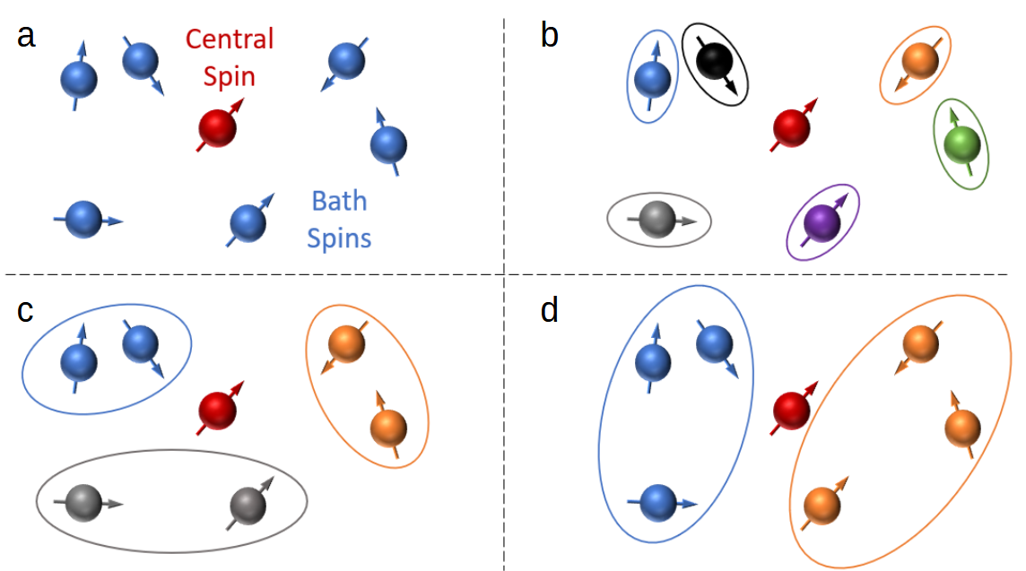
Figure S3: Illustration of different partitioning of a system: a) sketch of the spin system: a central spin (red) interacting with a spin bath (blue). b) - d) the spin bath is partitioned into local subsystems (partitions) each containing one (b), two (c) and three (d) spins. The partitions are indicated by ovals and different colors. The configuration in (b) corresponds to the conventional CCE method ($K=1$), whereas (c) and (d) correspond to the novel pCCE method with $K=2$ and $K=3$, respectively.

After finding the partitions, they represent indivisible units for the pCCE method. Clusters are formed based on the partitions. For example, pCCE(2,4) means that clusters are formed from one or two partitions with 4 and $2\cdot 4=8$ spins, respectively.

When investigating P1-center baths, we choose the following partitioning of the bath to increase the efficiency of the method: Each of the five subsystems within the P1-center bath introduced above is partitioned separately. This procedure avoids the situation when spins from different subsystems (which do not flip-flop with each other) enter the same partition. We checked whether this partitioning of the bath yields accurate results by partitioning (for some of the settings) the whole P1-center bath without paying attention to the subgroups. Both approaches lead to similar results.

The pCCE method is compatible with the gCCE approach (see, for example, Ref. [54]), which includes the central spin in each cluster. In fact, in order to use canonical typicality mentioned above, we used in our calculations the gCCE approach which is equivalent to the conventional CCE method for the systems considered.

To obtain the quantum-mechanical time-evolution operator from a Hamiltonian, we use the scipy.linalg.expm function from the scipy library. This function is based on the method described in Ref. [64].

VI Parameters of the pCCE method for large spin baths

In this section, we discuss the values of parameters for the pCCE method used in our calculations.

VI.1 Bath parameters

In our numerical simulations, we first create a very large diamond lattice with the NV-center in the center of this lattice and distribute P1-centers randomly on this lattice. P1-center spins sufficiently far away from the NV spin should have a negligible effect on the spin-coherence decay of the NV spin. Therefore, we limit the number of P1-center spins included in the simulation. We do this by introducing a bath radius $r_{\text{b}}$ which defines a sphere around the NV spin. Only spins within this sphere are considered dynamical.

Another parameter is the dipole radius $r_{\text{d}}$ which limits the distance between the partitions to form a joint cluster. The idea behind the dipole radius $r_{\text{d}}$ is that flip-flop transitions between spins from partitions far away from each other can be neglected. For the CCE approach, this corresponds to the distance between the respective spins. In the pCCE approach, the distance between two partitions is taken as the distance between the respective center points obtained from the constrained k-means algorithm (see above). Both parameters $r_{\text{b}}$ and $r_{\text{d}}$ need to be adjusted to each system considered.

Around the sphere of radius $r_{\text{b}}$ described above, we include further P1-center spins within a spherical shell of thickness $\frac{2}{3}r_{\text{d}}$ on the mean-field level, i.e., they are static. These additional spins are particularly important for spins close to the boundary of the sphere of radius of $r_{\text{b}}$. This means that, in total, we cut out a sphere of radius $r_{\text{b}}+\frac{2}{3}r_{\text{d}}$ from the large diamond lattice mentioned above and consider only spins within this sphere in our simulations.

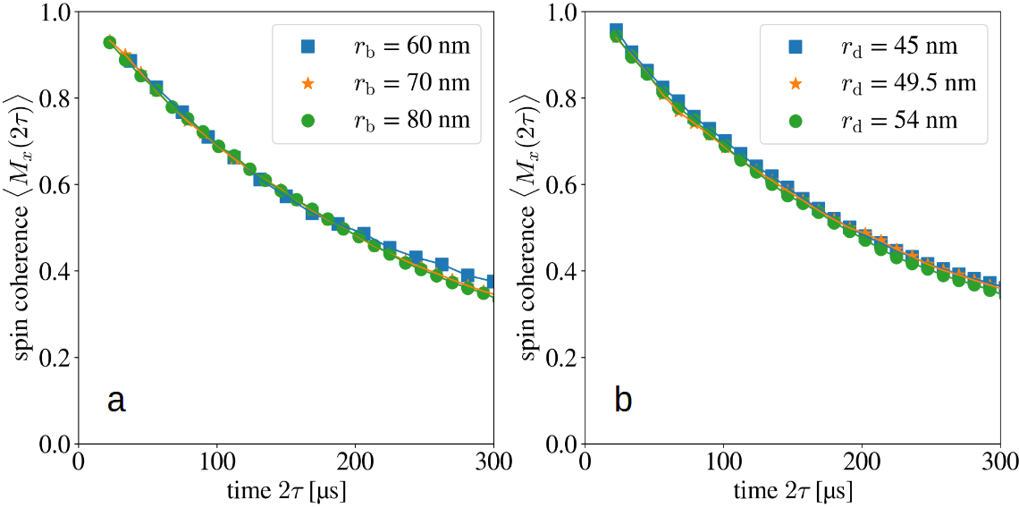
Figure S4: Evidence for the convergence of parameters for the pCCE(2,4) method applied to a large bath of P1-center electron spins in a quasi two-dimensional configuration at a concentration of 1 ppm: a) the bath-radius $r_{\text{b}}$ and b) the dipole radius $r_{\text{d}}$. The values of $r_{\text{b}}$ and $r_{\text{d}}$ depend both on the layer thickness $L$ and the bath-spin concentration $\rho_{\text{P1}}$. In our calculations, we choose the values for the parameters $r_{\text{b}}$ and $r_{\text{d}}$ corresponding to converged spin-coherence decay results, i.e., the spin-coherence decay does not change appreciably when increasing any of the parameters. For further details, see text.

The values of the above parameters $r_{\text{b}}$ and $r_{\text{d}}$ were determined in convergence studies. An example is illustrated in Fig. S4, where the spin-coherence decay $\langle M_{x}(2\tau)\rangle$ of the NV spin is shown for a P1-center spin bath at concentration 1 ppm using pCCE(2,4). The spin-coherence decay $\langle M_{x}(2\tau)\rangle$ is averaged over 100 randomly distributed spin systems and 20 mean-field spin configurations in internal averaging. The bath radius is increased in steps of 10 nm starting from 60 nm, see Fig. S4 a. The dipole radius is increased in steps of 10% starting from the initial value of 45 nm, see Fig. S4 b. In both calculations, the other parameter was kept constant at its initial value. The resulting graphs do not show any significant changes when varying the parameter values. We thus use the values $r_{\text{b}}=60$ nm and $r_{\text{d}}=45$ nm in our simulations for this particular system. Within the radius $r_{\text{b}}=60$ nm, there are 140 bath spins, which corresponds to the number of P1-centers. Small fluctuations of results shown in Fig. S4 arise presumably due to a finite number of samples for the mean-field average. The chosen parameter values are similar to those used in other studies of NV spins in P1-center baths for CCE2, see for example Ref. [48].

When considering other concentrations $\rho_{\text{P1}}$, the bath radius $r_{\text{b}}$ is chosen such that there are at least 140 spins, i.e., P1-centers, within the radius. To assure partitions of the same size within each P1-bath subgroup (discussed above), further spins are added to each subgroup until the total number of spins is divisible by the partition size $K$.

The dipole radius $r_{\text{d}}$ is, in general, a function of the concentration $\rho_{\text{P1}}$. We thus define

$$\tilde{r}_{\text{d}}(\rho_{\text{P1}})\equiv r_{\text{d,1}}\left(\frac{\rho_{\text{P1}}}{1\ \text{ppm}}\right)^{-1/3},$$ (S11)

where $r_{\text{d,1}}$ is the dipole radius at 1 ppm. To incorporate the effect of different spatial dimensionalities of the bath, we set

$$r_{\text{d}}(L,\rho_{\text{P1}})=\tilde{r}_{\text{d}}(\rho_{\text{P1}})\max\left[1,\sqrt{\frac{2\tilde{r}_{\text{d}}(\rho_{\text{P1}})}{L}}\right],$$ (S12)

where the last term on right-hand-side makes $r_{\text{d}}$ larger for quasi two-dimensional layers. We also use the same values of $r_{\text{b}}$ and $r_{\text{d}}$ when leaving out the hyperfine interaction in the P1-centers.

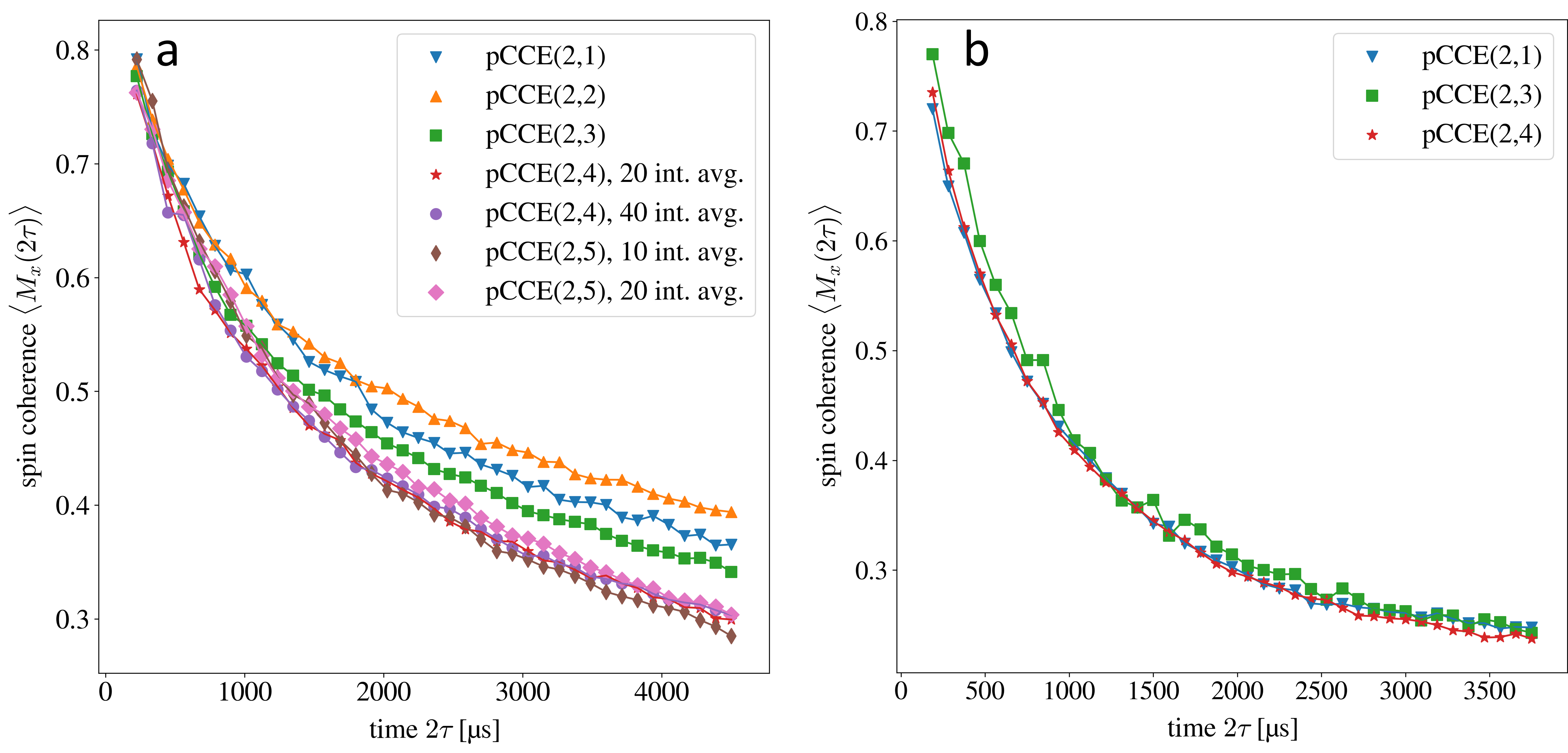
Figure S5: Convergence of the pCCE method with respect to the partition size $K$ and the number of samples for the internal mean-field average for different spin baths. a) An electron spin-1/2 bath in a quasi two-dimensional layer of thickness $L=5$ nm at a concentration of 1 ppm. At larger $K$, results for different numbers of samples for the internal average are also shown to demonstrate the convergence with the number of samples. b) A P1-center spin bath in a quasi two-dimensional layer ($L=30$ nm) at a concentration of $\rho_{\text{P1}}=1$ ppm. Fluctuation of results of pCCE(2,3) likely arise due to insufficient internal mean-field averaging. In a and b, the results for $K=2$ and $K=3$ were averaged internally over 100 and 50 mean-field samples, respectively.

VI.2 Partition size $K$ and the number of samples for the mean-field average

We first consider a quasi two-dimensional system of electron spins-1/2 with layer thickness $L=5$ nm and concentration of 1 ppm and calculate the spin-coherence decay $\langle M_{x}(2\tau)\rangle$. Figure S5 a shows results for different partition sizes $K$ and different number of samples for the internal mean-field average. The results indicate that the convergence is achieved for partition size $K=4$ and 20 samples for the internal mean-field average.

The decay of $\langle M_{x}(2\tau)\rangle$ becomes faster for larger $K$. This implies that, when using CCE2, the resulting $T_{2}$ time is too large in the quasi two-dimensional case. On the other hand, when considering three-dimensional baths of electron spins-1/2, the pCCE(2,$K$) results for all $K\geq 1$ demonstrate similar behaviour (not shown here) which indicates that already pCCE(2,1) (equivalent to CCE2) provides accurate results. For the sake of consistency, we use pCCE(2,4) also for these systems with the same number of samples for the internal average.

For the P1-center spin baths, no significant difference between pCCE(2,1) and pCCE(2,4) was observed for all layers, as indicated in Fig. S5 b. We attribute this to the strong suppression of flip-flop transitions in the bath due to the hyperfine interaction, see the first section of this supplemental material. The CCE2 method thus yields sufficiently accurate results for P1-center spin baths. However, this is strictly speaking valid only for the spin-coherence decay averaged over many different random spin distributions. This does not imply that, for each individual spin system, CCE2 yields sufficiently accurate results, cf. Ref. [53]. Using pCCE, accurate results can also be obtained for individual systems. It is also noteworthy, that, for establishing the validity of CCE2 approch for P1-center spin baths, the extensive use of the pCCE method was necessary.

VII Comparison with the conventional CCE method

We apply CCE3 to the bath of 20 electron spins-1/2 in a quasi two-dimensional layer considered in Fig. 2 of the main article. We vary the number of samples for internal averaging to mitigate the unphysical behavior $\langle M_{x}(2\tau)\rangle>1$; the results are shown in Fig. S6. The results imply that, with increasing number of samples for the internal mean-field average, no enhancement of the accuracy is achieved because the results do not converge even after averaging over 1000 samples. We conclude that this small bath of pure electron spins-1/2 in quasi two dimensions represents a challenging system for the conventional CCE method requiring a large number of samples for the mean-field average.

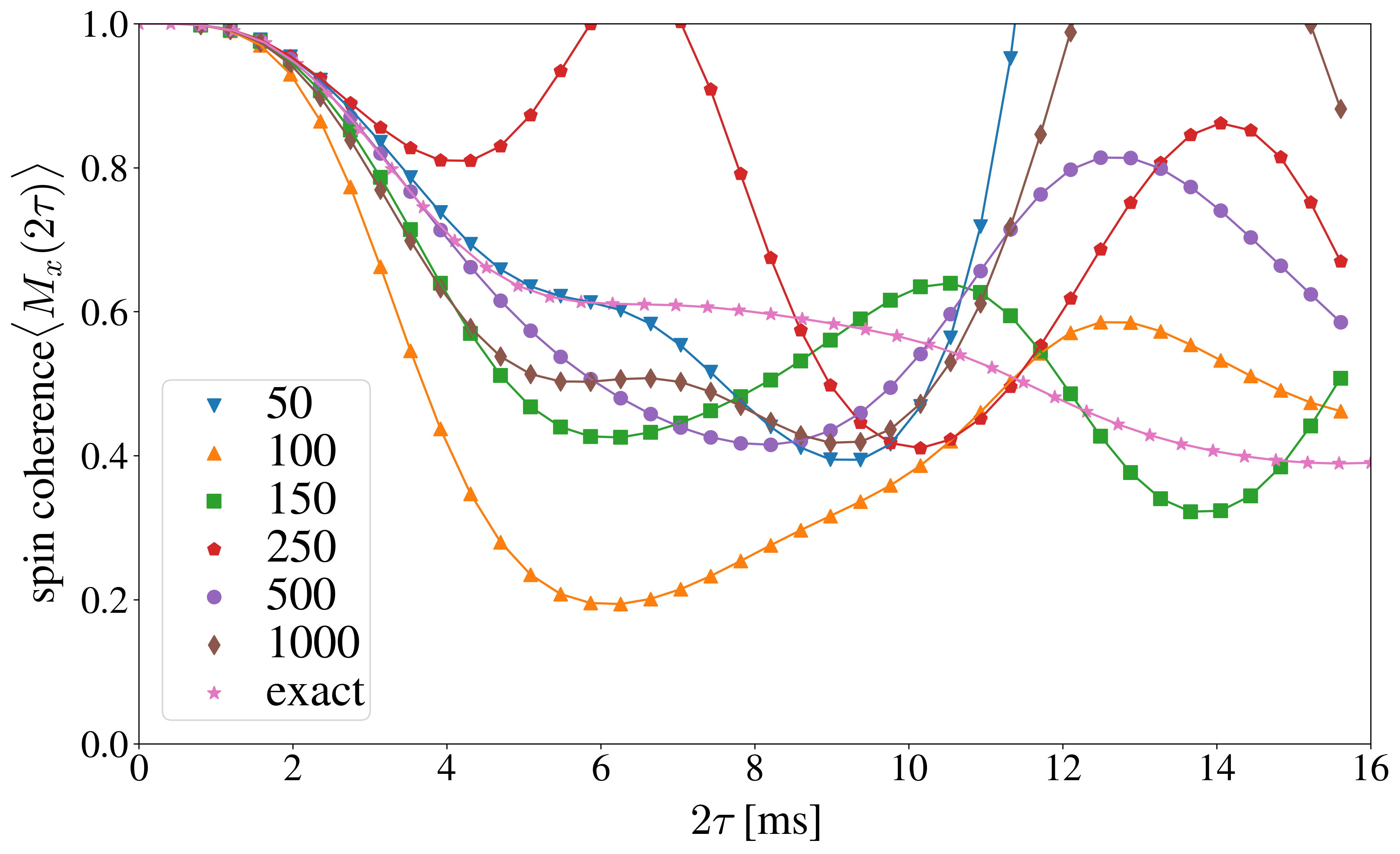
Figure S6: Results of CCE3 applied to the 20 electron spin-1/2 bath in a quasi two-dimensional layer (from Fig. (2)) for different numbers of samples for the internal average as indicated in the legend. At 1000 samples for the internal average, the CCE3 results have not converged and no signatures of convergence can be observed.

Table S1: Statistics for the occurrence of unphysical behavior ($\langle M_{x}(2\tau)\rangle>1$) for CCE3. We consider a series of smaller systems that we obtain by retaining only the 5, 10 or 15 closest spins to the NV-center from the system of 20 electron spins in a quasi two-dimensional layer, shown in Fig. 2 of the main article. These calculations were repeated 50 times and the fraction indicated in this table refers to this number of repetitions.

Number of spins	Occurrence of $\langle M_{x}(2\tau)\rangle$ > 1
5	0 %
10	28 %
15	26 %
20	40 %

We assume that the problem of unphysical behaviour ($\langle M_{x}(2\tau)\rangle>1$) becomes worse with increasing system size because, in larger spin baths, even more clusters are formed, each of which can lead to $\langle M_{x}(2\tau)\rangle>1$. To challenge this assumption, we consider a series of smaller systems that we obtain by retaining only the 5, 10 or 15 closest spins to the NV-center from the system of 20 electron spins considered in Fig. S6. We use CCE3, fix the number of samples for the internal mean-field average to 250 and count the occurrence of unphysical behavior, i.e., $\langle M_{x}(2\tau)\rangle>1$, while repeating the same calculation with random choices of the mean-field bath-spin configurations. The probability for the occurrence of such behavior increases with larger system size as shown in Table S1.

The above results imply that, even if the conventional CCE method of high order $N$ yields accurate results for the system considered in this article, this would involve a very large number of samples for the mean-field average. The pCCE method allows to increase the order $K$ while reducing the number of samples for the mean-field average. If we were to use the conventional CCE approach such that it includes all terms entering the pCCE(2,4) order, this would require CCE8 leading to a huge number of samples for the internal mean-field average provided such high-order CCE converges, cf. Ref. [53].

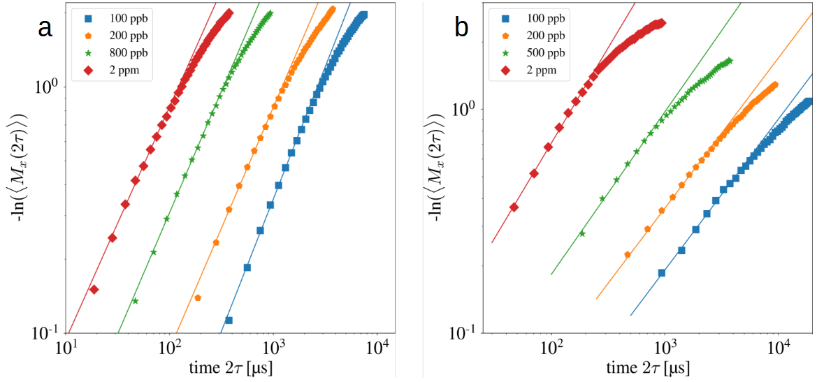
Figure S7: Illustration of the fitting of the stretched-exponential function in Eq. (2) to the numerical results shown in Fig. 3 at $L=240$ nm (a) and $L=60$ nm (b). The fitting parameters are the stretched-exponential parameter $p$ and the $T_{2}$ time. The slope of the linear curves and, hence, the parameter $p$ increases with increasing P1-center spin concentration $\rho_{\text{P1}}$ as indicated in the legend. The time window for the fit was adjusted for each individual curve separately.

VIII Fitting the stretched-exponential function

The stretched-exponential parameter $p$ and the characteristic $T_{2}$ time are extracted by fitting the stretched-exponential function in Eq. (2) to the short-time decay of the spin coherence $\langle M_{x}(2\tau)\rangle$. We perform a linear fit to $\ln(-\ln(\langle M_{x}(2\tau)\rangle))$ as a function of $\ln(t)$, from which we extract the slope corresponding to $p$, as illustrated in Fig. S7 for P1-center spin baths. Additionally, we extract the y-axis offset $d$. The $T_{2}$ time can then be calculated via $T_{2}=\exp\left(-\frac{d}{p}\right)$. We adjust the time window for the linear fit for each decay curve separately. We extend the time window to late times until a significant bending towards a smaller slope is observed. This bending usually occurs when $\langle M_{x}(2\tau)\rangle$ decayed below 0.6.

Similar behavior is observed for the baths of P1-centers without the hyperfine interaction, i.e., baths of electron spins-1/2. The resulting curves and corresponding fits are shown in Fig. S8. The transitions from three-dimensional to quasi two-dimensional systems occur at lower layer thickness compared to the P1-center spin bath. The reason for this is the absence of the suppression of the flip-flop transitions by the hyperfine interaction and, hence, different spin dynamics in the bath. Therefore, in Table 1 of the main text, we considered for the quasi two-dimensional configuration for P1-centers a layer thickness of $L=30\,$nm at 2 ppm and 1 ppm and $L=60\,$nm at 0.1 ppm, and, for P1-centers without the hyperfine interaction, $L=5\,$nm at 2 ppm and $L=10\,$nm at 0.1 ppm and 1 ppm.

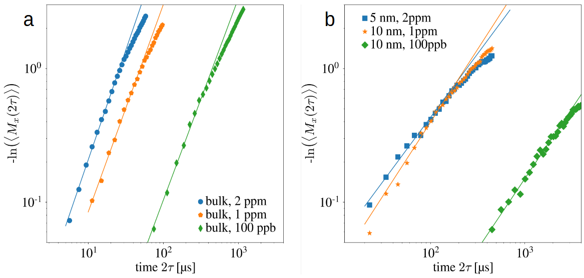
Figure S8: Illustration of the fitting of the stretched-exponential function in Eq. (2) to the numerical results obtained for P1-centers without the hyperfine interaction for three-dimensional (a) and quasi two-dimensional (b) diamond layers, cf. Table 1 of the main article. The layer thickness $L$ and the P1-center concentration $\rho_{\text{P1}}$ are indicated in the legends. The fitting parameters are the stretched-exponential parameter $p$ and the $T_{2}$ time. The time window for the fit was adjusted for each individual curve separately.

In general, we find that the decay of $\langle M_{x}(2\tau)\rangle$ comprises three regimes. At very small times, we observe a slope corresponding to a higher stretched-exponential parameter $p>1.5$. This is followed by the regime, which we refer to as the short-time decay. Here, we perform the linear fit as indicated in Figs. S7 and S8. Finally, the late-time decay is characterized by a lower stretched exponential, which can also be recognized by the bending of the curves in Fig. 3 of the main text, cf. Ref. [23].

The above three regimes complicate the choice for a suitable region for the fit of the short-time decay of $\langle M_{x}(2\tau)\rangle$. Thus, it is difficult to reliably identify the beginning and the end of this region such that the obtained slope of the curves corresponding to the stretched-exponential parameters $p$ together with the characteristic $T_{2}$ time must be considered an approximation. We estimate the error of each individual stretched-exponential parameter $p$ obtained to be at least $\pm$0.1.

References

- Slichter [1990] C. P. Slichter, Principles of Magnetic Resonance (Springer-Verlag, 1990).
- Abragam [1961] A. Abragam, Principles of Nuclear Magnetism (Oxford University Press, 1961).
- Anderson and Weiss [1953] P. W. Anderson and P. R. Weiss, Exchange narrowing in paramagnetic resonance, Rev. Mod. Phys. 25, 269 (1953).
- Klauder and Anderson [1962] J. R. Klauder and P. W. Anderson, Spectral diffusion decay in spin resonance experiments, Phys. Rev. 125, 912 (1962).
- Zhidomirov and Salikhov [1969] G. M. Zhidomirov and K. M. Salikhov, Contribution to the theory of spectral diffusion in magnetically diluted solids, Soviet Physics JETP 29, 1037 (1969).
- de Lange et al. [2010] G. de Lange, Z. H. Wang, D. Ristè, V. V. Dobrovitski, and R. Hanson, Universal dynamical decoupling of a single solid-state spin from a spin bath, Science 330, 60 (2010).
- Witzel et al. [2014] W. M. Witzel, K. Young, and S. Das Sarma, Converting a real quantum spin bath to an effective classical noise acting on a central spin, Phys. Rev. B 90, 115431 (2014).
- de Sousa and Das Sarma [2003] R. de Sousa and S. Das Sarma, Theory of nuclear-induced spectral diffusion: Spin decoherence of phosphorus donors in Si and GaAs quantum dots, Phys. Rev. B 68, 115322 (2003).
- Yao et al. [2006] W. Yao, R.-B. Liu, and L. J. Sham, Theory of electron spin decoherence by interacting nuclear spins in a quantum dot, Phys. Rev. B 74, 195301 (2006).
- Hanson et al. [2008] R. Hanson, V. V. Dobrovitski, A. E. Feiguin, O. Gywat, and D. D. Awschalom, Coherent dynamics of a single spin interacting with an adjustable spin bath, Science 320, 352 (2008).
- Hall et al. [2014] L. T. Hall, J. H. Cole, and L. C. L. Hollenberg, Analytic solutions to the central-spin problem for nitrogen-vacancy centers in diamond, Phys. Rev. B 90, 075201 (2014).
- Jeske et al. [2012] J. Jeske, J. H. Cole, C. Müller, M. Marthaler, and G. Schön, Dual-probe decoherence microscopy: probing pockets of coherence in a decohering environment, New Journal of Physics 14, 023013 (2012).
- Jeske and Cole [2013] J. Jeske and J. H. Cole, Derivation of markovian master equations for spatially correlated decoherence, Phys. Rev. A 87, 052138 (2013).
- Witzel and Das Sarma [2006] W. M. Witzel and S. Das Sarma, Quantum theory for electron spin decoherence induced by nuclear spin dynamics in semiconductor quantum computer architectures: Spectral diffusion of localized electron spins in the nuclear solid-state environment, Phys. Rev. B 74, 035322 (2006).
- Saikin et al. [2007] S. K. Saikin, W. Yao, and L. J. Sham, Single-electron spin decoherence by nuclear spin bath: Linked-cluster expansion approach, Phys. Rev. B 75, 125314 (2007).
- Yang and Liu [2008] W. Yang and R. B. Liu, Quantum many-body theory of qubit decoherence in a finite-size spin bath, Phys. Rev. B 78, 1 (2008).
- Maze et al. [2008a] J. R. Maze, J. M. Taylor, and M. D. Lukin, Electron spin decoherence of single nitrogen-vacancy defects in diamond, Phys. Rev. B 78, 094303 (2008a).
- Yang et al. [2016] W. Yang, W.-L. Ma, and R.-B. Liu, Quantum many-body theory for electron spin decoherence in nanoscale nuclear spin baths, Reports on Progress in Physics 80, 016001 (2016).
- Jeske et al. [2013] J. Jeske, N. Vogt, and J. H. Cole, Excitation and state transfer through spin chains in the presence of spatially correlated noise, Phys. Rev. A 88, 062333 (2013).
- Atatüre et al. [2018] M. Atatüre, D. Englund, N. Vamivakas, S.-Y. Lee, and J. Wrachtrup, Material platforms for spin-based photonic quantum technologies, Nature Reviews Materials 3, 38 (2018).
- Dowling and Milburn [2003] J. P. Dowling and G. J. Milburn, Quantum technology: the second quantum revolution, Philosophical Transactions of the Royal Society of London. Series A: Mathematical, Physical and Engineering Sciences 361, 1655 (2003).
- Awschalom et al. [2018] D. D. Awschalom, R. Hanson, J. Wrachtrup, and B. B. Zhou, Quantum technologies with optically interfaced solid-state spins, Nature Photonics 12, 516 (2018).
- Davis et al. [2023] E. J. Davis, B. Ye, F. Machado, S. A. Meynell, W. Wu, T. Mittiga, W. Schenken, M. Joos, B. Kobrin, Y. Lyu, Z. Wang, D. Bluvstein, S. Choi, C. Zu, A. C. B. Jayich, and N. Y. Yao, Probing many-body dynamics in a two-dimensional dipolar spin ensemble, Nature Physics 19, 836 (2023).
- Degen et al. [2017] C. L. Degen, F. Reinhard, and P. Cappellaro, Quantum sensing, Rev. Mod. Phys. 89, 035002 (2017).
- Doherty et al. [2013] M. W. Doherty, N. B. Manson, P. Delaney, F. Jelezko, J. Wrachtrup, and L. C. Hollenberg, The nitrogen-vacancy colour centre in diamond, Physics Reports 528, 1 (2013).
- Wrachtrup and Jelezko [2006] J. Wrachtrup and F. Jelezko, Processing quantum information in diamond, Journal of Physics: Condensed Matter 18, S807 (2006).
- Pezzagna and Meijer [2021] S. Pezzagna and J. Meijer, Quantum computer based on color centers in diamond, Applied Physics Reviews 8, 011308 (2021).
- Abobeih et al. [2018] M. H. Abobeih, J. Cramer, M. A. Bakker, N. Kalb, M. Markham, D. J. Twitchen, and T. H. Taminiau, One-second coherence for a single electron spin coupled to a multi-qubit nuclear-spin environment, Nature Communications 9, 2552 (2018).
- Abobeih et al. [2019] M. H. Abobeih, J. Randall, C. E. Bradley, H. P. Bartling, M. A. Bakker, M. J. Degen, M. Markham, D. J. Twitchen, and T. H. Taminiau, Atomic-scale imaging of a 27-nuclear-spin cluster using a quantum sensor, Nature 576, 411 (2019).
- Yao et al. [2012] N. Y. Yao, L. Jiang, A. V. Gorshkov, P. C. Maurer, G. Giedke, J. I. Cirac, and M. D. Lukin, Scalable architecture for a room temperature solid-state quantum information processor, Nature Communications 3 (2012).
- Morton and Lovett [2011] J. J. Morton and B. W. Lovett, Hybrid solid-state qubits: The powerful role of electron spins, Annual Review of Condensed Matter Physics 2, 189 (2011).
- Maze et al. [2008b] J. R. Maze, P. L. Stanwix, J. S. Hodges, S. Hong, J. M. Taylor, P. Cappellaro, L. Jiang, M. V. Dutt, E. Togan, A. S. Zibrov, A. Yacoby, R. L. Walsworth, and M. D. Lukin, Nanoscale magnetic sensing with an individual electronic spin in diamond, Nature 455, 644 (2008b).
- Barry et al. [2020] J. F. Barry, J. M. Schloss, E. Bauch, M. J. Turner, C. A. Hart, L. M. Pham, and R. L. Walsworth, Sensitivity optimization for NV-diamond magnetometry, Rev. Mod. Phys. 92, 15004 (2020).
- Gaebel et al. [2006] T. Gaebel, M. Domhan, I. Popa, C. Wittmann, P. Neumann, F. Jelezko, J. R. Rabeau, N. Stavrias, A. D. Greentree, S. Prawer, et al., Room-temperature coherent coupling of single spins in diamond, Nature Physics 2, 408 (2006).
- Herbschleb et al. [2019] E. Herbschleb, H. Kato, Y. Maruyama, T. Danjo, T. Makino, S. Yamasaki, I. Ohki, K. Hayashi, H. Morishita, M. Fujiwara, et al., Ultra-long coherence times amongst room-temperature solid-state spins, Nature communications 10, 3766 (2019).
- Taminiau et al. [2014] T. H. Taminiau, J. Cramer, T. van der Sar, V. V. Dobrovitski, and R. Hanson, Universal control and error correction in multi-qubit spin registers in diamond, Nature nanotechnology 9, 171 (2014).
- Abobeih et al. [2022] M. H. Abobeih, Y. Wang, J. Randall, S. J. H. Loenen, C. E. Bradley, M. Markham, D. J. Twitchen, B. M. Terhal, and T. H. Taminiau, Fault-tolerant operation of a logical qubit in a diamond quantum processor, Nature 606, 884 (2022).
- Taminiau et al. [2012] T. H. Taminiau, J. J. T. Wagenaar, T. van der Sar, F. Jelezko, V. V. Dobrovitski, and R. Hanson, Detection and control of individual nuclear spins using a weakly coupled electron spin, Phys. Rev. Lett. 109, 137602 (2012).
- Rodgers et al. [2021] L. V. Rodgers, L. B. Hughes, M. Xie, P. C. Maurer, S. Kolkowitz, A. C. Bleszynski Jayich, and N. P. de Leon, Materials challenges for quantum technologies based on color centers in diamond, MRS Bulletin 46, 623 (2021).
- Ohno et al. [2012] K. Ohno, F. J. Heremans, L. C. Bassett, B. A. Myers, D. M. Toyli, A. B. Jayich, C. J. Palmstrøm, and D. D. Awschalom, Engineering shallow spins in diamond with nitrogen delta-doping, Applied Physics Letters 101, 082413 (2012).
- Hughes et al. [2023] L. B. Hughes, Z. Zhang, C. Jin, S. A. Meynell, B. Ye, W. Wu, Z. Wang, E. J. Davis, T. E. Mates, N. Y. Yao, K. Mukherjee, and A. C. Bleszynski Jayich, Two-dimensional spin systems in PECVD-grown diamond with tunable density and long coherence for enhanced quantum sensing and simulation, APL Materials 11, 021101 (2023).
- Schätzle et al. [2023] P. Schätzle, P. Reinke, D. Herrling, A. Götze, L. Lindner, J. Jeske, L. Kirste, and P. Knittel, A chemical vapor deposition diamond reactor for controlled thin-film growth with sharp layer interfaces, physica status solidi (a) 220, 2200351 (2023).
- Ye et al. [2019] M. Ye, H. Seo, and G. Galli, Spin coherence in two-dimensional materials, npj Computational Materials 5, 44 (2019).
- Dwyer et al. [2022] B. L. Dwyer, L. V. Rodgers, E. K. Urbach, D. Bluvstein, S. Sangtawesin, H. Zhou, Y. Nassab, M. Fitzpatrick, Z. Yuan, K. De Greve, E. L. Peterson, H. Knowles, T. Sumarac, J.-P. Chou, A. Gali, V. Dobrovitski, M. D. Lukin, and N. P. de Leon, Probing spin dynamics on diamond surfaces using a single quantum sensor, PRX Quantum 3, 040328 (2022).
- Fel’dman and Lacelle [1996] E. B. Fel’dman and S. Lacelle, Configurational averaging of dipolar interactions in magnetically diluted spin networks, The Journal of Chemical Physics 104, 2000 (1996).
- Lacelle and Tremblay [1993] S. Lacelle and L. Tremblay, What is a typical dipolar coupling constant in a solid?, The Journal of Chemical Physics 98, 3642 (1993).
- Hahn and Dobrovitski [2021] W. Hahn and V. V. Dobrovitski, Long-lived coherence in driven spin systems: from two to infinite spatial dimensions, New Journal of Physics 23, 073029 (2021).
- Park et al. [2022] H. Park, J. Lee, S. Han, S. Oh, and H. Seo, Decoherence of nitrogen-vacancy spin ensembles in a nitrogen electron-nuclear spin bath in diamond, npj Quantum Information 8, 95 (2022).
- Sun and Cappellaro [2022] W. K. C. Sun and P. Cappellaro, Self-consistent noise characterization of quantum devices, Phys. Rev. B 106, 155413 (2022).
- Hahn [1950] E. L. Hahn, Spin echoes, Phys. Rev. 80, 580 (1950).
- [51] See Supplemental Material below.
- Witzel et al. [2010] W. M. Witzel, M. S. Carroll, A. Morello, L. Cywiński, and S. Das Sarma, Electron spin decoherence in isotope-enriched silicon, Phys. Rev. Lett. 105, 187602 (2010).
- Witzel et al. [2012] W. M. Witzel, M. S. Carroll, L. Cywiński, and S. Das Sarma, Quantum decoherence of the central spin in a sparse system of dipolar coupled spins, Phys. Rev. B 86, 035452 (2012).
- Onizhuk et al. [2021] M. Onizhuk, K. C. Miao, J. P. Blanton, H. Ma, C. P. Anderson, A. Bourassa, D. D. Awschalom, and G. Galli, Probing the coherence of solid-state qubits at avoided crossings, PRX Quantum 2, 010311 (2021).
- Seo et al. [2016] H. Seo, A. L. Falk, P. V. Klimov, K. C. Miao, G. Galli, and D. D. Awschalom, Quantum decoherence dynamics of divacancy spins in silicon carbide, Nature Communications 7, 12935 (2016).
- Suzuki et al. [1977] M. Suzuki, S. Miyashita, and A. Kuroda, Monte carlo simulation of quantum spin systems. I, Progress of Theoretical Physics 58, 1377 (1977).
- Bauch et al. [2020] E. Bauch, S. Singh, J. Lee, C. A. Hart, J. M. Schloss, M. J. Turner, J. F. Barry, L. M. Pham, N. Bar-Gill, S. F. Yelin, and R. L. Walsworth, Decoherence of ensembles of nitrogen-vacancy centers in diamond, Phys. Rev. B 102, 134210 (2020).
- Note [1] Interestingly, the obtained values are consistent with analytical expectations for double electron-electron resonance (DEER) experiments [45, 46, 47].
- [59] https://github.com/walter-hahn/pCCE-FraunhoferIAF.
- Davies [1981] G. Davies, The Jahn-Teller effect and vibronic coupling at deep levels in diamond, Reports on Progress in Physics 44, 787 (1981).
- Gemmer et al. [2009] J. Gemmer, M. Michel, and G. Mahler, Quantum Thermodynamics (Springer-Verlag, Berlin, 2009).
- Goldstein et al. [2006] S. Goldstein, J. L. Lebowitz, R. Tumulka, and N. Zanghì, Canonical typicality, Phys. Rev. Lett. 96, 050403 (2006).
- Levy-Kramer [2018] J. Levy-Kramer, k-means-constrained (2018).
- Al-Mohy and Higham [2010] A. H. Al-Mohy and N. J. Higham, A new scaling and squaring algorithm for the matrix exponential, SIAM Journal on Matrix Analysis and Applications 31, 970 (2010).