Hartman Effect from a Geometrodynamic Extension of Bohmian Mechanics

Abstract

This paper presents the derivation of a general solution to the scattering problem of particles incident onto a barrier of constant potential. This solution is constructed through a geometrodynamic approach to Bohmian mechanics, assuming that particles undergo quantum tunneling along geodesic trajectories in an Alcubierre-type spacetime. Furthermore, from this solution, mathematical expressions for the quantum potential, momentum, position, and tunneling time are determined in terms of the spacetime geometry for each relevant region. This allows us to explain the Hartman effect as a consequence of spacetime distortion generated by the quantum potential within the barrier.

I Introduction

The unusual saturation behavior in tunneling times discovered by Hartman in 1962, known as the Hartman Effect Hartman196200 , exhibited by particles incident upon a very wide potential barrier Sakurai2011 ; Zettili200900 ; Landauer198900 , has led to the contemplation of potential superluminal tunneling speeds Longhi200100 ; Winful200200 ; Winful200300 ; Sokolovski200000 . Initially, this sparked a vigorous debate regarding whether these results were due to inaccuracies in tunneling time measurements Ramos202000 . Subsequently, it compelled numerous theorists of the time to embark on the intricate task of addressing the fundamental question: What is the correct definition of tunneling time? Buttiker198300 ; Hauge198700 ; Winful200301 ; Winful200400 ; Winful200600 ; Rivlin202100 ; Rivlin202101 ; Petersen201700 . This question, captivating not only for physicists of that era but also relevant to contemporary researchers, has endured through the years, with many attempts to answer it proving unsuccessful across various approaches Winful200400 ; Winful200600 ; Martinez200600 ; Lantigua202300 .

Despite the considerable body of literature addressing this age-old paradox, existing work primarily focuses on definitions derived from approaches in relativistic and non-relativistic quantum mechanics. As previously mentioned, these approaches fall short of providing a satisfactory explanation for the observed effect Bandopadhyay200400 ; Delgado200300 ; Goldberg196700 ; Hauge198700 ; Muga199200 ; Hasan202000 ; Hasan202100 ; Winful200301 ; Winful200400 ; Martinez200600 ; Winful200600 ; Bandopadhyay202101 ; Lantigua202300 ; Leavens198900 . In contrast to these previous approaches, within the context of Bohmian mechanics, the question of defining tunneling time has not been sufficiently addressed Hagmann199300 ; Norsen201300 , despite a considerable body of literature on the application of Bohmian theory to the particle scattering problem over a potential barrier Norsen201300 . One of the more intriguing works in this context addresses a similar question and investigates Klein tunneling times for electrons in a two-terminal graphene device comprising a potential barrier between two metallic contacts Winful200600 ; Pandey201900 .

On the other hand, due to the mathematical structure of Bohmian mechanics Barut198800 ; Dewdney198700 ; Sole201600 , it is possible, through certain physical and mathematical considerations, to extend it to a version that incorporates elements of spacetime as defined in general relativity Gron200700 ; Janssen201300 . Therefore, it becomes feasible to develop a geometrodynamic description of quantum systems and to derive mathematical expressions that are not provided by approaches based on the orthodox formalism of relativistic or non-relativistic quantum theory Gomez201900 . Consequently, this work presents the construction of a solution that explains the Hartman Effect through a geometrodynamic approach to Bohmian mechanics, considering a spacetime endowed with a metric that allows for superluminal travel without violating the principles of general relativity Alcubierre199400 .

More specifically, the present work reports a general solution constructed under the hypothesis that particles, during the tunneling phenomenon, follow geodesic trajectories within an Alcubierre-type spacetime Alcubierre199400 ; Santos202000 . Consequently, from this solution, quantities of interest are determined, including mathematical expressions describing linear momenta, quantum potentials, and particle positions for the problem under investigation. As a result, the particle’s position expression leads to the mathematical expression of the tunneling time, equipped with the geometric elements of the considered spacetime.

The remainder of this article is organized as follows. Section II provides a brief yet necessary review of the fundamental concepts of Bohmian mechanics. Section III deduces the geometrodynamic version of the quantum force based on the results presented in Ref. Gomez201900 . Section IV presents the construction of the general solution to the problem of a particle incident from the left on a barrier of constant potential for each of the regions of interest. In Section V, the general expression of the quantum potential for each region of interest is determined. Section VI establishes the general expression for linear momentum and particle position, again for each region of interest, consequently providing the mathematical expression for the tunneling time. Section VII presents the conclusion of the work. We also include an Appendix containing the mathematical results and some methods used in the main text.

II Fundamentals of Bohmian mechanics

Bohmian mechanics is a theory discovered by Louis De Broglie in 1927 and later rediscovered by David Bohm in 1952. It provides a description of quantum systems through a mathematical object known as the wave function, which encodes their dynamics Dewdney198700 . In essence, the partial description of the quantum system is given by a wave function that satisfies the quantum equilibrium hypothesis and evolves according to the Schrödinger equation. Meanwhile, the particles’ evolution is described by the guiding equation, which outlines their velocities in terms of this wave function Barut198800 ; Oriols201900 .

In presenting the foundational mathematical framework of Bohmian mechanics, we consider the following wave function:

$$\Psi=\sqrt{\rho}\exp{\{iS\}},$$ (1)

where $\rho\equiv\rho(\vec{x},t)$ and $S\equiv S(\vec{x},t)$. Upon substituting this function into the Schrödinger equation,

$$\biggl{[}-\frac{\hbar^{2}}{2m}\nabla^{2}+V\biggr{]}\Psi=i\hbar\partial_{t}\Psi,$$ (2)

we obtain the expressions:

$$-\frac{\hbar^{2}}{2m}\frac{\nabla^{2}\sqrt{\rho}}{\sqrt{\rho}}+\frac{\hbar^{2}}{2m}(\nabla S)^{2}+V=-\hbar\partial_{t}S$$ (3)

and

$$-\frac{\hbar^{2}}{2m}\biggl{[}2(\nabla\sqrt{\rho})\cdot\nabla S+\sqrt{\rho}(\nabla^{2}S)\biggr{]}=\hbar\partial_{t}\sqrt{\rho}.$$ (4)

Furthermore, using the equalities $2\sqrt{\rho}(\nabla\sqrt{\rho})=\nabla\rho$ and $2\sqrt{\rho}(\partial_{t}\sqrt{\rho})=\partial_{t}\rho$, we can multiply Eq. (4) by $2\sqrt{\rho}$ to obtain:

$$\partial_{t}\rho+\frac{\hbar}{m}\nabla\cdot(\rho\nabla S)=0.$$ (5)

Additionally, recalling that the probability current density is defined as $\vec{j}\equiv\rho\vec{v}=\Psi^{\ast}\Psi\vec{v}$, we can determine the expression for particle velocity by substituting Eq. (1) into:

$$\Psi^{\ast}\Psi\vec{v}=\frac{i\hbar}{2m}\biggl{[}\Psi\nabla\Psi^{\ast}-\Psi^{\ast}\nabla\Psi\biggr{]},$$ (6)

resulting in:

$$\vec{v}=(\hbar/m)\nabla S.$$ (7)

This allows us to rewrite equations (3) and (5) as:

$$\hbar\partial_{t}S+\frac{\hbar^{2}}{2m}(\nabla S)^{2}+V+Q=0$$ (8)

and

$$\partial_{t}\rho+\nabla\cdot\vec{j}=0,$$ (9)

where we introduced the quantity

$$Q\equiv-\hbar^{2}(\nabla^{2}\sqrt{\rho})/(2m\sqrt{\rho}),$$ (10)

referred to as the quantum potential or Bohmian potential, and $\vec{j}\equiv\rho[\hbar(\nabla S)/m]$. In other words, equations (8) and (9) are the differential equations describing the behavior of $S$ and $\rho$ Pena200600 .

Finally, to complete the formalism, the gradient of Eq. (8) is calculated, and the result is expressed in terms of the velocity field (7) to obtain:

$$m\partial_{t}\vec{v}+m(\vec{v}\cdot\nabla)\vec{v}=-\nabla(V+Q)=\vec{F}+\vec{F}_{Q}.$$ (11)

The above expression is the equation of motion that a particle with a probability current density given by Eq. (6) will follow under the action of an effective force $\vec{F}=\vec{F}_{V}+\vec{F}_{Q}$. Therefore, in the classical limit ($\hbar\rightarrow 0$), the trajectories will obey the laws of Newtonian motion, as expected Dewdney198700 ; Barut198800 ; Pena200600 ; Oriols201900 .

III Geometrodynamics and Quantum Force

When considering the extension of Bohmian mechanics to a relativistic version, several seemingly insurmountable challenges arise. For instance, issues include extending Bohmian trajectories to relativistic paths, constructing a four-vector of probability density and current, and dealing with non-physical trajectory occurrences—especially concerning photons—due to frames of reference where velocity is zero. However, through careful physical and mathematical considerations, it is possible to construct geometrodynamic models that allow for such an extension Gomez201900 . Therefore, this section presents a deduction of the quantum force equation in curvilinear coordinates. In other words, it derives a generalized version of the quantum force expression presented in Ref. Gomez201900 . The procedure followed here essentially mirrors that of the authors in that work, and their contributions play a central role in constructing the solution presented in this article.

One possible connection between Bohmian mechanics and general relativity arises by postulating that particles in the quantum system follow geodesic trajectories in spacetime. This hypothesis can be expressed mathematically through the following expression:

$$0=\frac{d^{2}x^{\mu}}{dt^{2}}+\Gamma^{\mu}_{\alpha\beta}\frac{dx^{\alpha}}{dt}\frac{dx^{\beta}}{dt},$$ (12)

where $\mu$, $\alpha$, and $\beta$ take values in $\{0,1,2,3\}$. Equation (12) yields the geometrodynamic constraint:

$$\Gamma^{0}_{\alpha\beta}\frac{dx^{\alpha}}{dt}\frac{dx^{\beta}}{dt}=0.$$ (13)

This establishes a local equivalence relation between the Euclidean spacetime where Bohmian mechanics is defined and the spacetime of the Lorentzian manifold by considering $x^{0}=ct$ Gomez201900 . Therefore, by considering $j,k,\mu=i=1,2,3$ and $\alpha,\beta=0,1,2,3$, equation (12) can be developed to obtain:

$$0=\frac{d^{2}x^{i}}{dt^{2}}+\Gamma^{i}_{jk}\frac{dx^{j}}{dt}\frac{dx^{k}}{dt}-2c\Gamma^{i}_{0j}\frac{dx^{j}}{dt}+c^{2}\Gamma^{i}_{00}.$$ (14)

Considering the components of the gradient in a generally curved space, given by

$$(\nabla f)^{i}=\frac{g^{ij}}{\sqrt{|g|}}\partial_{j}f,$$ (15)

where $|g|=|\det(g_{\mu\nu})|$, allows the rewriting of expressions for the potential gradients as

$$(\nabla V)^{i}=\frac{g^{ij}}{\sqrt{|g|}}\partial_{j}V$$ (16)

and

$$(\nabla Q)^{i}=\frac{g^{ij}}{\sqrt{|g|}}\partial_{j}Q.$$ (17)

Furthermore, the mathematical expression for acceleration in a general system of orthogonal coordinates is given by

$$\ddot{x}^{i} =\frac{d^{2}x^{i}}{dt^{2}}+G^{i}_{jk}\partial x^{j}\partial x^{k}$$

$$=\frac{d^{2}x^{i}}{dt^{2}}+\omega^{i}.$$ (18)

Above $G_{jk}^{i}$ are the Christoffel symbols in the orthogonal coordinate system. Then, considering the expressions (16), (17), and (III), equation (11) is reformulated as:

$$\Gamma^{i}_{jk}\frac{dx^{j}}{dt}\frac{dx^{k}}{dt}-2c\Gamma^{i}_{0j}\frac{dx^{j}}{dt}+c^{2}\Gamma^{i}_{00}$$

$$=\omega^{i}+\frac{g^{ij}}{m\sqrt{|g|}}\partial_{j}V+\frac{g^{ij}}{m\sqrt{|g|}}\partial_{j}Q.$$ (19)

Next, considering the general expression for the momentum components, $(\vec{P})^{i}=\hbar(\nabla S)^{i}$, which, similarly to (16) or (17), can be rewritten as

$$P^{i}=\frac{\hbar g^{ij}}{\sqrt{|g|}}\partial_{j}S\;\;\rightarrow\;\;\frac{dx^{i}}{dt}=\frac{\hbar g^{ij}}{m\sqrt{|g|}}\partial_{j}S.$$ (20)

Using the Christoffel symbols

$$\Gamma^{i}_{jk} =\frac{g^{ih}}{2}\{\partial_{j}g_{hk}+\partial_{k}g_{jh}-\partial_{h}g_{jk}\},$$

$$\Gamma^{i}_{j0} =\frac{g^{ih}}{2}\{\partial_{j}g_{h0}+\partial_{0}g_{jh}-\partial_{h}g_{j0}\},$$

$$\Gamma^{i}_{00} =\frac{g^{ih}}{2}\{2\partial_{0}g_{h0}-\partial_{h}g_{00}\},$$ (21)

the expression (III) is recast as follows:

$$\frac{\hbar^{2}g^{ih}}{2(m\sqrt{|g|})^{2}}\{\partial_{j}g_{hk}+\partial_{k}g_{jh}-\partial_{h}g_{jk}\}g^{jl}g^{kn}\partial_{l}S\partial_{n}S$$

$$-\frac{c\hbar g^{ih}}{m\sqrt{|g|}}\{\partial_{j}g_{h0}+\partial_{0}g_{jh}-\partial_{h}g_{j0}\}g^{jl}\partial_{l}S$$

$$+\frac{c^{2}g^{ih}}{2}\{2\partial_{0}g_{h0}-\partial_{h}g_{00}\}$$

$$=\omega^{i}+\frac{g^{il}}{m\sqrt{|g|}}\partial_{l}V+\frac{g^{il}}{m\sqrt{|g|}}\partial_{l}Q.\;$$ (22)

The expression (22) represents a geometrodynamic extension of the quantum force in Eq. (11) Gomez201900 . In simple terms, it provides an extended mathematical formalism that allows the description of physical systems based on their geometric evolution, where the central mathematical object of Bohmian theory (the wave function) maintains its prominent role. Moreover, in this geometrodynamic extension, not only does the wave function preserve its central role as the entity encoding the system’s dynamics, but, in this formalism, the particle and the wave function, which are well-defined and clearly distinct entities, assume a dialectical role.

IV Construction of the General Solution to the Problem

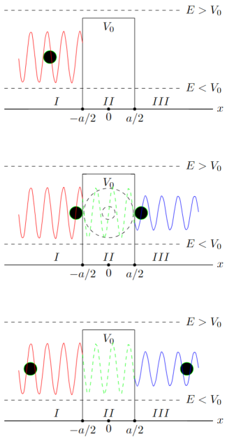
In this section, we present the deduction of the Bohmian solution to the one-dimensional problem of particle scattering incident from the left on a constant potential barrier Pena200600 ; Zettili200900 ; Sakurai2011 , based on the direct application of the formalism introduced in the previous sections II and III. For this reason, we will consider the following three regions of interest. The first one is denoted as $I$, where the particle is incident, guided by its pilot wave, and subsequently reflected or not. The second region is denoted as $II$, bounded by the potential barrier, where quantum tunneling phenomenon occurs. Finally, the last region considered is denoted as $III$, where particle transmission, with its corresponding pilot wave, occurs. See Fig. 1.

Figure 1: Schematic representation of the tunneling of a particle with energy $E$, incident from the left on a potential barrier of height $V_{0}$ and width $a$. Additionally, in this representation, the regions $I$, $II$, and $III$ are identified, which are considered in the construction of the general solution presented in section IV.

Therefore, the Schrödinger equation for the problem represented in Figure 1 can be written as follows:

$$d_{x}^{2}\psi(x)+[k^{2}-\xi^{2}\Theta(x-a/2)\Theta(a/2-x)]\psi(x)=0,$$ (23)

where $\xi^{2}=2V_{0}$, $k^{2}=2E$, $\hbar=1$, $c=1$, and $m=1$. When solved, this equation allows finding the wave function $\psi(x)$ used in the Bohmian formalism Dewdney198700 ; Barut198800 ; Pena200600 ; Oriols201900 . Additionally, it is considered that the potential barrier has a width $a$ and a height $V_{0}$, and is mathematically defined as:

$$V(x)=V_{0}\Theta(x-a/2)\Theta(a/2-x).$$ (24)

Here $\Theta$ is the Heaviside step function, which is mathematically defined as:

$$\Theta(x)=\begin{cases}0&\mbox{for }x<0\\ 1&\mbox{for }x\geq 0\end{cases}.$$ (25)

Thus, the solution in regions $I$ and $III$ are given by the expressions:

$$\psi_{I}(x) =A^{\prime}e^{ikx}+B^{\prime}e^{-ikx}\ \text{for}\ x\leq-a/2,$$ (26)

$$\psi_{III}(x) =F^{\prime}e^{ikx}\ \text{for}\ x\geq a/2,$$ (27)

which, when written in the form (1), reduce to the expressions:

$$\Psi_{I}(x) =\sqrt{\rho_{I}}\exp{\{iS_{I}(x)\}}\ \text{for}\ x\leq-a/2,$$ (28)

$$\Psi_{III}(x) =\sqrt{\rho_{III}}\exp{\{iS_{III}(x)\}}\ \text{for}\ x\geq a/2,$$ (29)

where $\sqrt{\rho_{I}}=\sqrt{\mathcal{A}^{2}\cos^{2}{kx}+\mathcal{B}^{2}\sin^{2}{kx}}$ with $\mathcal{A}=A^{\prime}+B^{\prime}$ and $\mathcal{B}=i(A^{\prime}-B^{\prime})$, $\sqrt{\rho_{III}}=F^{\prime}=\mathcal{F}$, $S_{I}(x)=\tan^{-1}{\{[\mathcal{B}\tan{kx}]/\mathcal{A}\}}$, and $S_{III}(x)=kx$.

However, to obtain a consistent Bohmian solution for this problem, temporal dependence in the wave function must be included, as shown in Ref. Dewdney198700 . That is to say, we consider $\Psi_{I}(x,t)=\Psi_{I}(x)\exp{\{iEt\}}$ and $\Psi_{III}(x,t)=\Psi_{III}(x)\exp{\{iEt\}}$. Thus, we can write the general solution for regions $I$ and $III$ as a superposition of solutions with different energy eigenstates:

$$\Psi_{j}(x,t)=\sum_{l=1}^{2}C_{j}^{l}\sqrt{\rho_{j}^{l}}\exp{\{i[S_{j}^{l}(x)-E^{l}t]\}}.$$ (30)

Next, the general solution can be rewritten in the form of the Bohmian wave function, where the phase functions depending on position and time are given by:

$$S_{j}(x,t)=\tan^{-1}{\left(\frac{\sum_{l=1}^{2}C_{j}^{l}\sqrt{\rho_{j}^{l}}\sin{\Omega_{j}^{l}(x,t)}}{\sum_{l=1}^{2}C_{j}^{l}\sqrt{\rho_{j}^{l}}\cos{\Omega_{j}^{l}(x,t)}}\right)},$$ (31)

with $\Omega_{j}^{l}(x,t)=S_{j}^{l}(x)-E^{l}t$ and

$$\sqrt{\rho_{j}}=\sqrt{\sum_{l=1}^{2}(C_{j}^{l})^{2}\rho_{j}^{l}+2C_{j}^{q}C_{j}^{q+1}\sqrt{\rho_{j}^{q}\rho_{j}^{q+1}}\cos{\Xi_{j}^{q}}},$$ (32)

with $\Xi_{j}^{1}\equiv\Xi_{j}(x,t)=S_{j}^{2}(x)-S_{j}^{1}(x)-(E^{2}-E^{1})t$ and $q=1$.

However, the solution in region $II$ is obtained by solving the equation (22) considering the Alcubierre metric tensor Alcubierre199400 ; Alcubierre200500 given by

$$g_{\mu\nu} =\begin{pmatrix}v_{s}^{2}f^{2}(r_{s})-1&-v_{s}f(r_{s})&0&0\\ -v_{s}f(r_{s})&1&0&0\\ 0&0&1&0\\ 0&0&&1\end{pmatrix},$$ (33)

whose inverse tensor is given by the expression

$$g^{\mu\nu}=\begin{pmatrix}-1&-v_{s}f(r_{s})&0&0\\ -v_{s}f(r_{s})&1-v_{s}^{2}f^{2}(r_{s})&0&0\\ 0&0&1&0\\ 0&0&0&1\end{pmatrix},$$ (34)

where $v_{s}\equiv v_{s}(t)=\dot{x}_{s}(t)$, $f(r_{s})=\alpha_{0}/\{v_{s}[1+\alpha_{1}\cosh{(2\sigma r_{s})}]\}$, $r_{s}\equiv r_{s}(t)=x-x_{s}(t)$, and $x_{s}(t)=nct=nt$, since in this article $c=1$. On the other hand, it is important to note that in the problem addressed here, a constant potential, $V=V_{0}$, is considered, and due to the structure of the metric tensor (33), we have $\omega^{i}=0$ for $i=1,2,3$ and $\partial_{l}V=0$. For this reason, the following set of equations is obtained from equation (22):

$$\begin{split}&\frac{c^{2}g^{10}\partial_{0}g_{00}}{2}+\frac{c^{2}g^{11}\{2\partial_{0}g_{10}-\partial_{1}g_{00}\}}{2}=-\frac{g^{11}\partial_{1}Q}{m\sqrt{|g|}}\;\;\mbox{for}\;i=1,\ j\neq 1,\\ &\frac{c\hbar g^{10}(\partial_{1}g_{00})\partial_{1}S}{m\sqrt{|g|}}-\frac{g^{11}\partial_{1}Q}{m\sqrt{|g|}}=-\frac{g^{11}\partial_{1}Q}{m\sqrt{|g|}}\;\;\mbox{for}\;i=j=1,\ k\neq 1,\\ &\frac{\hbar^{2}g^{01}(2\partial_{1}g_{01})(g^{11})^{2}(\partial_{1}S)^{2}}{2(m\sqrt{|g|})^{2}}-\frac{c\hbar g^{10}(\partial_{1}g_{00})g^{11}\partial_{1}S}{m\sqrt{|g|}}-\frac{g^{11}\partial_{1}Q}{m\sqrt{|g|}}=-\frac{g^{11}\partial_{1}Q}{m\sqrt{|g|}}\;\;\mbox{for}\;i=j=k=1.\;\end{split}$$ (35)

Next, by considering the nontrivial solutions of (35), the expression

$$dS =-2dr_{s}v_{s}f\left\{\frac{1}{1-v^{2}_{s}f^{2}}\right\},$$ (36)

is deduced, which allows calculating the phase function in region $II$. Similarly, the expression

$$dQ =df\left\{\frac{v_{s}}{1-v_{s}^{2}f^{2}}+v_{s}^{2}f\right\}$$ (37)

is obtained, whose solution will be presented later, allowing us to obtain the expression for the quantum potential in region $II$. Therefore, by integrating (36), as shown in part $I$ of the Appendix, the phase function is obtained:

$$S_{II}(x,x_{s}(t)) =\frac{\alpha_{0}\beta_{0}}{2\sigma\sqrt{(\beta_{3})^{2}-(\beta_{2})^{2}}}$$ (38)

$$\times\Biggl{\{}\frac{\beta_{1}-\mu_{0}}{\sqrt{\mu_{0}}}\tan^{-1}{\Biggl{[}\frac{1}{\sqrt{\mu_{0}}}\tan{\frac{x^{\prime}}{2}}\Biggr{]}}$$

$$\hskip 14.22636pt-\frac{\beta_{1}-\mu_{1}}{\sqrt{\mu_{1}}}\tan^{-1}{\Biggl{[}\frac{1}{\sqrt{\mu_{1}}}\tan{\frac{x^{\prime}}{2}}\Biggr{]}}\Biggr{\}}.$$

Above $\alpha_{0}=-[v_{s}\tanh{(2\sigma R)}]/[2\tanh{(\sigma R)}]$, $\alpha_{1}=\mbox{sech}{(2\sigma R)}$, $\beta_{0}=[2(\alpha_{1}-1)]/[(\alpha_{1}-1)^{2}-\alpha^{2}_{0}]$, $\beta_{1}=(\alpha_{1}+1)/(\alpha_{1}-1)$, $\beta_{2}=[(\alpha_{1}+1)^{2}-\alpha^{2}_{0}]/[(\alpha_{1}-1)^{2}-\alpha^{2}_{0}]$, $\beta_{3}=[\alpha_{1}^{2}-1+\alpha^{2}_{0}]/[(\alpha_{1}-1)^{2}-\alpha^{2}_{0}]$, $\mu_{0}=\beta_{3}-\sqrt{(\beta_{3})^{2}-(\beta_{2})^{2}}$, $\mu_{1}=\beta_{3}+\sqrt{(\beta_{3})^{2}-(\beta_{2})^{2}}$ and

$$x^{\prime} =\cos^{-1}{\left[\mbox{sech}{(2\sigma r_{s})}\right]}.$$ (39)

However, it is important to note that physically acceptable solutions for (36), leading to a consistent phase function (38), are those where $\alpha_{1}\neq 0$ or $\alpha_{1}\neq 1$. Then, by imposing the continuity conditions of the solution and of its derivatives, the expressions obtained from (30) must be substituted into

$$\Psi_{k}(x,t)\biggl{|}_{(x_{k},t_{k})}=\Psi_{k+I}(x,t)\biggl{|}_{(x_{k},t_{k})},$$ (40)

$$[\partial_{x}\Psi_{k}(x,t)]\biggl{|}_{(x_{k},t_{k})}=[\partial_{x}\Psi_{k+I}(x,t)]\biggl{|}_{(x_{k},t_{k})}$$ (41)

with $x_{k}\in\{-a/2,a/2$ }, $t_{k}\in\{t_{0},t_{1}\}$ and $k=I,II,III$. Thus one obtains the system of equations:

$$\mathcal{C}_{I}^{1}\zeta_{1}+\mathcal{C}_{I}^{2}\zeta_{2}e^{i\Delta Et_{0}}=\zeta_{3}[\mathcal{C}_{II}^{1}+\mathcal{C}_{II}^{2}e^{i\Delta Et_{0}}],$$

$$\mathcal{C}_{I}^{1}\zeta_{1}^{\prime}+\mathcal{C}_{I}^{2}\zeta_{2}^{\prime}e^{i\Delta Et_{0}}=\zeta_{3}^{\prime}[\mathcal{C}_{II}^{1}+\mathcal{C}_{II}^{2}e^{i\Delta Et_{0}}],$$

$$\mathcal{C}_{III}^{1}\zeta_{5}+\mathcal{C}_{III}^{2}\zeta_{6}e^{i\Delta Et_{1}}=\zeta_{4}[\mathcal{C}_{II}^{1}+\mathcal{C}_{II}^{2}e^{i\Delta Et_{1}}],$$

$$\mathcal{C}_{III}^{1}\zeta_{5}^{\prime}+\mathcal{C}_{III}^{2}\zeta_{6}^{\prime}e^{i\Delta Et_{1}}=\zeta_{4}^{\prime}[\mathcal{C}_{II}^{1}+\mathcal{C}_{II}^{2}e^{i\Delta Et_{1}}].$$ (42)

Consequently, by solving the system of equations (42) while imposing the superposition condition $\mathcal{C}_{II}^{2}=1-\mathcal{C}_{II}^{1}$, the expressions for the coefficients are obtained:

$$\mathcal{C}_{I}^{1}=\varpi_{4}e^{-i\Delta Et_{0}}[(e^{i\Delta Et_{0}}-1)\mathcal{C}_{II}^{1}+1],$$

$$\mathcal{C}_{I}^{2}=\varpi_{3}[(e^{i\Delta Et_{0}}-1)\mathcal{C}_{II}^{1}+1],$$

$$\mathcal{C}_{II}^{1}=-\frac{e^{i\Delta Et_{1}}}{e^{i\Delta Et_{1}}-1}\left\{\varpi_{2}\mathcal{C}_{III}^{1}-1\right\},$$

$$\mathcal{C}_{II}^{2}=\frac{1}{e^{i\Delta Et_{1}}-1}\left\{\varpi_{2}e^{i\Delta Et_{1}}\mathcal{C}_{III}^{1}-1\right\},$$

$$\mathcal{C}_{III}^{2}=\varpi_{1}e^{i\Delta Et_{1}}\mathcal{C}_{III}^{1}.$$ (43)

Above we defined $\varpi_{1}=[\zeta_{4}^{\prime}\zeta_{5}-\zeta_{4}\zeta_{5}^{\prime}]/[\zeta_{4}\zeta_{6}^{\prime}-\zeta_{4}^{\prime}\zeta_{6}]$, $\varpi_{2}=[\zeta_{5}^{\prime}\zeta_{6}-\zeta_{5}\zeta_{6}^{\prime}]/[\zeta_{4}\zeta_{6}^{\prime}-\zeta_{4}^{\prime}\zeta_{6}]$, $\varpi_{3}=[\zeta_{1}\zeta_{3}^{\prime}-\zeta_{1}^{\prime}\zeta_{3}]/[\zeta_{1}\zeta_{2}^{\prime}-\zeta_{1}^{\prime}\zeta_{2}]$ and $\varpi_{4}=[\zeta_{2}^{\prime}\zeta_{3}-\zeta_{2}\zeta_{3}^{\prime}]/[\zeta_{1}\zeta_{2}^{\prime}-\zeta_{1}^{\prime}\zeta_{2}]$ with

$$\zeta_{l}=\sqrt{\rho_{I}^{l}(x)}\exp{\{iS_{I}^{l}(x)\}}\biggl{|}_{(-1)^{l}\frac{a}{2}},$$

$$\zeta_{l}^{\prime}=[2\rho_{I}^{l}(x)]^{-1}k^{l}[(\mathcal{B}^{2}-\mathcal{A}^{2})\sqrt{\rho_{I}^{l}(x)}\sin{2k^{l}x}$$

$$+i2\mathcal{A}\mathcal{B}]e^{iS_{I}^{l}(x)}\biggl{|}_{(-1)^{l}\frac{a}{2}},$$

$$\zeta_{l+2}=\exp{\{i[S_{II}(x)+V_{0}t]\}}\biggl{|}_{((-1)^{l+2}\frac{a}{2},t_{0})},$$

$$\zeta_{l+2}^{\prime}=\frac{i\alpha_{0}\beta_{0}\sec^{2}{(\frac{x^{\prime}}{2})}\tan{(2\sigma r_{s})}e^{i[S_{II}(x)+V_{0}t]}}{2\sqrt{(\beta_{3})^{2}-(\beta_{2})^{2}}\sqrt{\cosh^{2}{(2\sigma r_{2})}-1}}$$

$$\times\biggl{[}\frac{\beta_{1}-\mu_{1}}{\mu_{1}+\tan^{2}{(\frac{x^{\prime}}{2})}}-\frac{\beta_{1}-\mu_{0}}{\mu_{0}+\tan^{2}{(\frac{x^{\prime}}{2})}}\biggr{]}\biggl{|}_{((-1)^{l+2}\frac{a}{2},t_{0})},$$

$$\zeta_{l+4}=\exp{\{iS_{III}^{l}(x)\}}\biggl{|}_{\frac{a}{2}},$$

$$\zeta_{l+4}^{\prime}=ik^{l}\exp{\{iS_{III}^{l}(x)\}}\biggl{|}_{\frac{a}{2}}.\;$$ (44)

In the expressions above, values for $l=1,2$ are considered, along with the energy variation $\Delta E=E^{2}-E^{1}$. Additionally, the coefficients were rewritten as $C_{j}^{l}=\mathcal{C}_{j}^{l}$ if $j=I$, and $C_{j}^{l}\sqrt{\rho_{j}^{l}}=\mathcal{C}_{j}^{l}$ if $j=II,III$, again for all $l=1,2$. In summary, through the coefficients presented in (43) and the expressions for $S_{I}^{l}$, $S_{II}$, and $S_{III}^{l}$, the general solution to the problem for each of the regions of interest can be written as:

$$\Psi_{I}(x,t) =\mathcal{C}_{I}^{1}\sqrt{\rho_{I}^{1}(x)}\exp{\{i[S_{I}^{1}(x)-E^{1}t]\}}$$

$$+\mathcal{C}_{I}^{2}\sqrt{\rho_{I}^{1}(x)}\exp{\{i[S_{I}^{2}(x)-E^{2}t]\}},$$

$$\Psi_{II}(x,t) =[\mathcal{C}_{II}^{1}\exp{\{-i[E^{1}-V_{0}]t\}}$$

$$+\mathcal{C}_{II}^{2}\exp{\{-i[E^{2}-V_{0}]t\}}]\exp{\{iS_{II}(x)\}},$$

$$\Psi_{III}(x,t) =\mathcal{C}_{III}^{1}\sqrt{\rho_{I}^{1}(x)}\exp{\{i[S_{III}^{1}(x)-E^{1}t]\}}$$

$$+\mathcal{C}_{III}^{2}\sqrt{\rho_{I}^{1}(x)}\exp{\{i[S_{III}^{2}(x)-E^{2}t]\}},$$ (45)

where, as expected, the general expression is written in terms of the geometry of the spacetime considered by imposing the geometrodynamic constraint (13). Then, by substituting $\mathcal{C}_{III}^{2}$ into the expression for $\sqrt{\rho_{III}}$, the transmission coefficient is obtained:

$$T =\mathcal{C}_{III}^{1}\sqrt{1+\varpi_{1}^{2}e^{i2\Delta Et_{1}}+2\varpi_{1}e^{i\Delta Et_{1}}\cos{\Xi_{III}}}.$$ (46)

V General Expression for the Quantum Potential

In this section, we apply the formalism and results presented in Sections II, III, and IV to deduce the general expression of the quantum potential for each of the regions considered in the problem of interest. To this end, it is necessary to calculate $Q_{j}=-(\nabla^{2}\sqrt{\rho_{j}})/(2\sqrt{\rho_{j}})$ in regions $I$ and $III$, while in region $II$, it is necessary to integrate the expression (37).

In this regard, obtaining an expression for region $I$ proves to be a challenging task due to the form of the general solution. Nevertheless, by rewriting $\sqrt{\rho_{j}^{l}}$ in the form

$$\begin{split}\sqrt{\rho_{j}^{l}}&=\sqrt{\mathcal{A}^{2}\cos^{2}{k^{l}x}+\mathcal{B}^{2}\sin^{2}{k^{l}x}}\\ &=\sqrt{(A^{\prime}+B^{\prime})^{2}\cos^{2}{k^{l}x}-(A^{\prime}-B^{\prime})^{2}\sin^{2}{k^{l}x}}\\ &=\sqrt{2A^{\prime}B^{\prime}+[(A^{\prime})^{2}+(B^{\prime})^{2}]\cos{2k^{l}x}},\;\end{split}$$ (47)

and considering the solution for low energies ($k^{l}x\approx 0\;\rightarrow\;\cos{2k^{l}x}\approx 1$), expression (47) simplifies to a more straightforward format given by

$$\begin{split}\sqrt{\rho_{j}^{l}}&=\sqrt{2A^{\prime}B^{\prime}+(A^{\prime})^{2}+(B^{\prime})^{2}}\\ &=\sqrt{(A^{\prime}+B^{\prime})^{2}}\\ &=\mathcal{A}.\;\end{split}$$ (48)

On the other hand, the phase function for low energies reduces to

$$S_{I}^{l}(x) =\tan^{-1}{\{[\mathcal{B}\tan{k^{l}x}]/\mathcal{A}\}}\approx\mathcal{B}k^{l}x/\mathcal{A}.\;$$ (49)

Hence, it is possible to rewrite (32) in terms of (48) and (49) to obtain the quantum potential in region I:

$$Q_{I}(x,t)=\biggl{[}\frac{\mathcal{B}(k^{2}-k^{1})}{\sqrt{2}\rho_{I}}\biggr{]}^{2}\{\rho_{I}\cos{\Xi_{I}}+\mathcal{A}\mathcal{C}_{I}^{1}\mathcal{C}_{I}^{2}\sin^{2}{\Xi_{I}}\},$$ (50)

with amplitude $\sqrt{\rho_{I}}=\mathcal{A}\sqrt{(\mathcal{C}_{I}^{1})^{2}+(\mathcal{C}_{I}^{2})^{2}+2\mathcal{C}_{I}^{1}\mathcal{C}_{I}^{2}\cos{\Xi_{I}}}$ and where the angle $\Xi_{I}=S_{I}^{2}(x)-S_{I}^{1}(x)-(E^{2}-E^{1})t$. Furthermore, since $\sqrt{\rho_{III}}$ differs from $\sqrt{\rho_{I}}$ only by the constants $\mathcal{A}$ and $\mathcal{B}$, it is not difficult to verify that the quantum potential in region $III$ is given by

$$Q_{III}(x,t) =\biggl{[}\frac{(k^{2}-k^{1})}{\sqrt{2}\rho_{III}}\biggr{]}^{2}\{\rho_{III}\cos{\Xi_{III}}$$ (51)

$$\hskip 73.97733pt+\mathcal{C}_{III}^{1}\mathcal{C}_{III}^{2}\sin^{2}{\Xi_{III}}\},$$

with amplitude

$$\sqrt{\rho_{III}}=\sqrt{(\mathcal{C}_{III}^{1})^{2}+(\mathcal{C}_{III}^{2})^{2}+2\mathcal{C}_{III}^{1}\mathcal{C}_{III}^{2}\cos{\Xi_{I}}},$$ (52)

and where the angle is given by

$$\Xi_{III}=S_{III}^{2}(x)-S_{III}^{1}(x)-(E^{2}-E^{1})t.$$ (53)

Unlike regions $I$ and $III$, and as mentioned in the previous section, the quantum potential in region $II$ is determined by integrating (37), resulting in the expression

$$Q_{II}(x,t) =\Biggl{\{}\ln{\Biggl{|}\frac{1+v_{s}f}{\sqrt{1-v^{2}_{s}f^{2}}}\Biggr{|}}+\frac{v^{2}_{s}f^{2}}{2}\Biggr{\}}.$$ (54)

VI Momentum, Position, and Tunneling Time

In the previous sections, along with the theoretical foundations and the general solution, we derived the mathematical expressions for the quantum potential in each of the regions of interest in our problem. Even though the wave function and the quantum potential are fundamental quantities within the framework of Bohmian mechanics Dewdney198700 ; Barut198800 ; Pena200600 ; Oriols201900 , it is essential to determine the particle’s momentum and position. Therefore, this section is dedicated to calculating the mathematical expressions for these quantities, ultimately allowing us to determine the quantum tunneling time Hartman196200 ; Buttiker198300 ; Hagmann199300 ; Winful200200 ; Winful200300 ; Winful200301 ; Winful200400 ; Winful200600 .

In order to determine the linear momentum in region $I$, we need to substitute the expressions (48) and (49) into (31) to obtain the phase function $S_{I}(x,t)$. Substituting this into (7), we obtain

$$P_{I}(x,t) =\{\mathcal{B}[(\mathcal{C}_{I}^{1})^{2}k^{1}+(\mathcal{C}_{I}^{2})^{2}k^{2}+\mathcal{C}_{I}^{1}\mathcal{C}_{I}^{2}(k^{1}$$ (55)

$$\hskip 14.22636pt+k^{2})\cos{\Xi_{I}}]\}\{\mathcal{A}[(\mathcal{C}_{I}^{1})^{2}+(\mathcal{C}_{I}^{2})^{2}$$

$$\hskip 65.44142pt+2\mathcal{C}_{I}^{1}\mathcal{C}_{I}^{2}\cos{\Xi_{I}}]\}^{-1}.$$

Analogously, setting $\mathcal{B}/\mathcal{A}=1$ in Eq. (49), we obtain the expressions for $S_{III}^{l}$. Rewriting Eq. (31) and substituting it into Eq. (7), we determine that the linear momentum in region $III$ is given by

$$P_{III}(x,t) =\{(\mathcal{C}_{III}^{1})^{2}k^{1}+(\mathcal{C}_{III}^{2})^{2}k^{2}+\mathcal{C}_{III}^{1}\mathcal{C}_{III}^{2}(k^{1}$$ (56)

$$\hskip 14.22636pt+k^{2})\cos{\Xi_{III}}\}\{(\mathcal{C}_{III}^{1})^{2}+(\mathcal{C}_{III}^{2})^{2}$$

$$\hskip 65.44142pt+2\mathcal{C}_{III}^{1}\mathcal{C}_{III}^{2}\cos{\Xi_{III}}\}^{-1}.$$

Alternatively, substituting Eq. (38) into Eq. (7) yields the linear momentum in region $II$, which is given by

$$P_{II}(x,t)=\frac{\alpha_{0}\beta_{0}\mbox{sech}(2\sigma r_{s})}{2\sqrt{(\beta_{3})^{2}-(\beta_{2})^{2}}}$$

$$\times\Biggl{\{}\frac{\beta_{1}-\mu_{0}}{\mu_{0}\cos^{2}{[\frac{\mbox{sech}(2\sigma r_{s})}{2}]}+\sin^{2}{[\frac{\mbox{sech}(2\sigma r_{s})}{2}]}}$$

$$-\frac{\beta_{1}-\mu_{1}}{\mu_{1}\cos^{2}{[\frac{\mbox{sech}(2\sigma r_{s})}{2}]}+\sin^{2}{[\frac{\mbox{sech}(2\sigma r_{s})}{2}]}}\Biggr{\}}.$$ (57)

As a result, the following differential equations are derived from the expressions (55) and (56):

$$\frac{dx}{dt} =\frac{\hbar\mathcal{B}}{m\mathcal{A}}\frac{\vartheta_{3}\{1+\vartheta_{4}\cos{\Xi_{I}}\}}{\vartheta_{1}\{1+\vartheta_{2}\cos{\Xi_{I}}\}},$$ (58)

$$\frac{dx}{dt} =\frac{\hbar}{m}\frac{\vartheta_{9}\{1+\vartheta_{10}\cos{\Xi_{III}}\}}{\vartheta_{11}\{1+\vartheta_{12}\cos{\Xi_{III}}\}},$$ (59)

where $\vartheta_{1}=(\mathcal{C}_{I}^{1})^{2}+(\mathcal{C}_{I}^{2})^{2}$, $\vartheta_{2}=2\mathcal{C}_{I}^{1}\mathcal{C}_{I}^{2}/[(\mathcal{C}_{I}^{1})^{2}+(\mathcal{C}_{I}^{2})^{2}]$, $\vartheta_{3}=(\mathcal{C}_{I}^{1})^{2}k^{1}+(\mathcal{C}_{I}^{2})^{2}k^{2}$, $\vartheta_{4}=\mathcal{C}_{I}^{1}\mathcal{C}_{I}^{2}(k^{1}+k^{2})/[(\mathcal{C}_{I}^{1})^{2}k^{1}+(\mathcal{C}_{I}^{2})^{2}k^{2}]$, $\vartheta_{9}=(\mathcal{C}_{III}^{1})^{2}k^{1}+(\mathcal{C}_{III}^{2})^{2}k^{2}$, $\vartheta_{10}=\mathcal{C}_{III}^{1}\mathcal{C}_{III}^{2}(k^{1}+k^{2})/[(\mathcal{C}_{III}^{1})^{2}k^{1}+(\mathcal{C}_{III}^{2})^{2}k^{2}]$, $\vartheta_{11}=(\mathcal{C}_{III}^{1})^{2}+(\mathcal{C}_{III}^{2})^{2}$ and $\vartheta_{12}=2\mathcal{C}_{III}^{1}\mathcal{C}_{III}^{2}/[(\mathcal{C}_{III}^{1})^{2}+(\mathcal{C}_{III}^{2})^{2}]$. In the same way, starting from Eq. (57), we obtain

$$\frac{dx}{dt} =\vartheta_{5}\left\{\frac{\vartheta_{6}\cosh^{3}{(2\sigma r_{s})}+\cosh{(2\sigma r_{s})}}{\cosh^{4}{(2\sigma r_{s})}+\vartheta_{7}\cosh^{2}{(2\sigma r_{s})}+\vartheta_{8}}\right\},$$ (60)

with

$$\begin{split}\vartheta_{5}&=\alpha_{0}\beta_{0}(\mu_{1}-\mu_{0})/[8\mu_{0}\mu_{1}\sqrt{(\beta_{3})^{2}-(\beta_{2})^{2}}],\\ \vartheta_{6}&=4\beta_{1},\\ \vartheta_{7}&=(\mu_{1}+\mu_{0})/4\mu_{0}\mu_{1},\\ \vartheta_{8}&=1/4\mu_{0}\mu_{1}.\end{split}$$ (61)

However, it is important to highlight that the above differential equation is obtained by considering $0\leq\mbox{sech}(2\sigma r_{s})/2\leq 1/2\;\;\rightarrow\;\;\cosh{[\mbox{sech}(2\sigma r_{s})/2]}\approx 1$ and $\sinh{[\mbox{sech}(2\sigma r_{s})/2]}\approx\mbox{sech}(2\sigma r_{s})/2$ in Eq. (57). This holds true for $\sigma\ll 1$ Alcubierre199400 . But what is the physical or mathematical reason behind this condition? The answer to this question arises when analyzing the expression $\alpha_{1}=1/\cosh{(2\sigma R)}=\mbox{sech}(2\sigma R)$ introduced in Section IV, from which we derive $\sigma=\mbox{arsech}(\alpha_{1})/2R$ and consequently $\mbox{arsech}(\alpha_{1})\ll 2R$. It is worthwhile mentioning that as the quantity $\mbox{arsech}(\alpha_{1})$ is a dimensionless constant, the above expression does not consider the units of $R$ or, in the particular case, $R_{e}$; that is, we only aim to establish a comparison in orders of magnitude.

Therefore, in order to provide a physical meaning to this last mathematical condition, particles of small dimensions, such as an electron, are considered, whose radius has the value $R_{e}=2.8178402894(58)\times 10^{-13}\,\text{m}$. Comparing it with the Bohr radius ($a_{0}=5.29177210903(86)\times 10^{-11}\,\text{m}$), we obtain the relation $a_{0}=188R_{e}$. Thus, it is sufficient to choose an $\alpha_{1}$ such that $R_{e}<\mbox{arsech}(\alpha_{1})\ll 376R_{e}$ to obtain an appropriate parameter $\sigma$. Consequently, by recalling that $v_{s}=n$ and considering $\alpha_{1}=2\rightarrow\sigma\ll 1$, the coefficients in Eq. (61) reduce to the expressions: $\vartheta_{5}=-\{15728640n[1-(3n/4)^{2}]\}/[10496-4483.84n^{2}+81n^{4}]$, $\vartheta_{6}=12$, $\vartheta_{7}=\{10240[1-(3n/4)^{2}]\sqrt{1+(2n/5)^{2}}\}/[10496-4483.84n^{2}+81n^{4}]$, and $\vartheta_{8}=\{81920[1-(3n/4)^{2}]^{2}\}/[10496-4483.84n^{2}+81n^{4}]$. Therefore, by solving the differential equations (58), (59), and (60) (see the Appendix), we obtain the expressions shown below:

$$\varrho_{I} =\frac{\vartheta_{3}^{\prime}[\vartheta_{3}^{\prime}-\vartheta_{1}]}{4[\vartheta_{3}^{\prime}\vartheta_{4}-\vartheta_{1}\vartheta_{2}]}\biggl{\{}\vartheta_{4}\Xi_{I}$$

$$+\frac{2\vartheta_{1}[\vartheta_{2}-\vartheta_{4}][\vartheta_{3}^{\prime}(1-\vartheta_{4})-\vartheta_{1}(1+\vartheta_{2})]^{\frac{1}{2}}}{[\vartheta_{3}^{\prime}(1-\vartheta_{4})-\vartheta_{1}(1-\vartheta_{2})]^{\frac{3}{2}}}\tan^{-1}{\biggl{[}\sqrt{\frac{\vartheta_{3}^{\prime}(1-\vartheta_{4})-\vartheta_{1}(1+\vartheta_{2})}{\vartheta_{3}^{\prime}(1-\vartheta_{4})-\vartheta_{1}(1-\vartheta_{2})}}\tan{\biggl{(}\frac{\Xi_{I}}{2}\biggr{)}}\biggr{]}}\biggr{\}},$$

$$\varrho_{II} =\frac{\vartheta_{6}^{\prime}+\vartheta_{5}}{1-\vartheta_{6}^{\prime}+\vartheta_{7}-\vartheta_{5}+\vartheta_{8}}r_{s}-\frac{2\sigma^{2}[\vartheta_{6}^{\prime}+(3\vartheta_{5}-\vartheta_{6}^{\prime}\vartheta_{7})+2\vartheta_{5}\vartheta_{6}^{\prime}+(\vartheta_{5}\vartheta_{7}-3\vartheta_{6}^{\prime}\vartheta_{8})-\vartheta_{5}\vartheta_{8}]}{3[1-\vartheta_{6}^{\prime}+\vartheta_{7}-\vartheta_{5}+\vartheta_{8}]^{2}}r_{s}^{3},$$

$$\varrho_{III} =\frac{\vartheta_{9}^{\prime}[\vartheta_{9}^{\prime}-\vartheta_{11}]}{4[\vartheta_{9}^{\prime}\vartheta_{10}-\vartheta_{11}\vartheta_{12}]}\biggl{\{}\vartheta_{10}\Xi_{III}$$

$$+\frac{2\vartheta_{11}[\vartheta_{12}-\vartheta_{10}][\vartheta_{9}^{\prime}(1-\vartheta_{10})-\vartheta_{11}(1+\vartheta_{12})]^{\frac{1}{2}}}{[\vartheta_{9}^{\prime}(1-\vartheta_{10})-\vartheta_{11}(1-\vartheta_{12})]^{\frac{3}{2}}}\tan^{-1}{\biggl{[}\sqrt{\frac{\vartheta_{9}^{\prime}(1-\vartheta_{10})-\vartheta_{11}(1+\vartheta_{12})}{\vartheta_{9}^{\prime}(1-\vartheta_{10})-\vartheta_{11}(1-\vartheta_{12})}}\tan{\biggl{(}\frac{\Xi_{III}}{2}\biggr{)}}\biggr{]}}\biggr{\}}.$$ (62)

Above we defined $\vartheta_{3}^{\prime}=\mathcal{B}\vartheta_{3}/\mathcal{A}$, $\vartheta_{9}^{\prime}=\vartheta_{9}$, and where $\varrho_{I}$, $\varrho_{II}$, and $\varrho_{III}$ are arbitrary constants. Then, as the expressions presented in Eq. (62) do not allow for solving one variable in terms of the other to obtain the general equation of trajectories for all time $t$, it is possible, at least, to provide an idea of such trajectories for the stationary case by plotting a set of isochronous curves. These curves are obtained by recalling that $\vartheta_{3}^{\prime}=\mathcal{B}\vartheta_{3}/\mathcal{A}=[A^{\prime}-B^{\prime}]\vartheta_{3}/[A^{\prime}+B^{\prime}]$, where $A^{\prime}$ and $B^{\prime}$ are arbitrary constants. This allows rewriting the first of the expressions in Eqs. (62) as the sum of two terms, one positive corresponding to incident particles and one negative corresponding to reflected particles. Thus, the graphical representation of the expressions (62) is obtained, as shown in Fig. 2.

Figure 2: Schematic representation of the trajectories followed by particles incident from the left on the potential barrier.

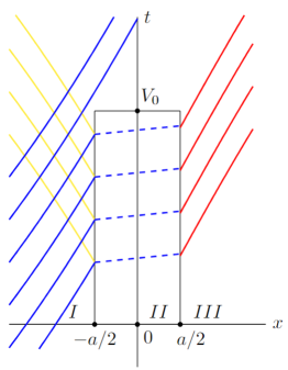
In Figure 2, trajectories of incident and reflected particles are depicted in blue and yellow, respectively, in region $I$. In region $II$, trajectories of tunneling particles are represented by a blue-dashed line. In region $III$, trajectories of transmitted particles are shown. It is essential to highlight that the trajectories presented in this plot correspond to the curves of the incident functions $f^{(i)}(x,t)=0.25(2.41x-nt)+\tan^{-1}{\{10\tan{[(2.41x-nt)/2]}\}}/10+\varrho_{I}^{(i)}$, reflected $f^{(r)}(x,t)=-0.25(2.41x-nt)-\tan^{-1}{\{10\tan{[(2.41x-nt)/2]}\}}/10+\varrho_{I}^{(r)}$, tunneling $f^{(tu)}(x,t)=0.0995(x-nt)+\varrho_{II}^{(tu)}$, and transmitted $f^{(tr)}(x,t)=0.25[2.41x-nt]+\tan^{-1}{\{10\tan{[(2.41x-nt)/2]}\}}/10+\varrho_{III}^{(tr)}$ (with arbitrary chosen values for the constants in each expression). Taking $n=2$, $t=1$, and the sets of values $\varrho_{I}^{(i)}=\{4.65,5.65,6.65,7.65,8.65,9.65\}$, $\varrho_{I}^{(r)}=\{-1.75,-0.75,0.25,1.25\}$, $\varrho_{II}^{(tu)}=\{1.75,2.75,3.75,4.75\}$, $\varrho_{III}^{(tr)}=\{1.3,2.3,3.3,4.3\}$, where the closest plots to the $x$-axis correspond to the first elements of each set of values and so on.

On the other hand, the determination of the tunneling time depends on a comprehensive analysis of some of the quantities of interest introduced in Ref. Alcubierre199400 , such as the four-velocity and the square of the line element. In particular, we begin with the analysis of the four-velocity of the Eulerian observer given by

$$u^{\mu} =(1,-v_{s}f,0,0),$$ (63)

whose covariant derivative allows us to obtain the expansion of the volume elements Alcubierre199400 produced by the bubble

$$\theta =u_{;\nu}^{\mu}=-v_{s}(\partial_{x}f),$$ (64)

and whose component $u^{1}=v$ mathematically expresses the speed with which the ‘warp’ bubble moves in the $ox$ direction. Consequently, due to the previous consideration $\alpha_{1}=2\rightarrow\sigma\ll 1$, we have that

$$v=-v_{s}\left[-\frac{v_{s}}{v_{s}(1+2)}\right]=\frac{v_{s}}{3}.$$ (65)

As $v_{s}$ can take arbitrary values, the ‘warp’ bubble is free to move at even superluminal speeds Alcubierre199400 . However, if the above statement holds true, the following question becomes valid: would we be in a situation where coordinate time is equal to proper time? The answer to this question arises from analyzing the square of the line element

$$ds^{2} =-dt^{2}+[dx-v_{s}fdt]^{2}+dy^{2}+dz^{2},$$ (66)

and what it implies to consider a particle inside the bubble moving along the curve $x=x_{s}(t)\rightarrow dx=v_{s}dt$ as the bubble moves through spacetime. Therefore, considering $dy=dz=0$ and $f=1$, we get

$$ds^{2}=-dt^{2}+[v_{s}dt-v_{s}dt]^{2}=-dt^{2}.$$ (67)

This leads to the following two implications. First, the fact that $ds^{2}<0$ implies that the curve representing the trajectory followed by the particle is of a time-like nature. Second, by rewriting (67), considering the definition of proper time, $d\tau^{2}=-ds^{2}$, we obtain

$$d\tau =dt,$$ (68)

which implies that the metric proposed in Refs. Alcubierre199400 ; Alcubierre200500 does not generate temporal dilations between the time measured with respect to the particle and the coordinate time.

For this reason, we consider a particle moving inside the ‘warp’ bubble Krasnikov199800 following the trajectory $x=x^{\prime}+vt=x^{\prime}+nt/3$ (with $v_{s}=n\rightarrow v=n/3$) and again $\sigma\ll 1$. With this, we can rewrite the second expression in Eq. (62) as follows

$$\varrho_{II} =\frac{\vartheta_{6}^{\prime}+\vartheta_{5}}{1-\vartheta_{6}^{\prime}+\vartheta_{7}-\vartheta_{5}+\vartheta_{8}}\biggl{(}x^{\prime}-\frac{2n}{3}t\biggr{)}.$$ (69)

Then, by evaluating Eq. (69) at the points $\mathcal{P}_{0}(-a/2,t_{0})$ and $\mathcal{P}_{1}(a/2,t_{1})$, we get

$$\varrho_{II} =\frac{\vartheta_{6}^{\prime}+\vartheta_{5}}{1-\vartheta_{6}^{\prime}+\vartheta_{7}-\vartheta_{5}+\vartheta_{8}}\biggl{(}-\frac{a}{2}-\frac{2n}{3}t_{0}\biggr{)}$$ (70)

and

$$\varrho_{II} =\frac{\vartheta_{6}^{\prime}+\vartheta_{5}}{1-\vartheta_{6}^{\prime}+\vartheta_{7}-\vartheta_{5}+\vartheta_{8}}\biggl{(}\frac{a}{2}-\frac{2n}{3}t_{0}\biggr{)},$$ (71)

which, when subtracted, gives us

$$\Delta t =\frac{3}{2n}a.$$ (72)

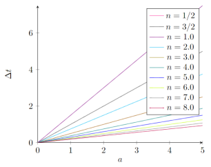
In other words, the tunneling time (72), graphically represented in Fig. 3, depends on the barrier width, as expected. That is, with an increase in the potential barrier width, the tunneling time could increase depending on the value of the tunneling velocity. This velocity could even reach superluminal regimes due to the distortion of spacetime, as seen in Eq. (11) or in Eq. (22), generated by the quantum potential of Eq. (54).

As a result, by choosing $v_{s}=n$ in this model, there is no saturation in the tunneling times obtained in Refs. Hartman196200 ; Winful200400 ; Winful200600 ; Lantigua202300 . Therefore, it can be said that the solution Eq. (45), constructed in this work, eliminates the apparent paradox by considering the Alcubierre-type spacetime inside the potential barrier, where particles follow geodesic trajectories. However, despite the general expression

$$\begin{split}\varrho_{II}&=\{\vartheta_{6}^{\prime}(v_{s})+\vartheta_{5}(v_{s})\}\{1-\vartheta_{6}^{\prime}(v_{s})+\vartheta_{7}(v_{s})\\ &-\vartheta_{5}(v_{s})+\vartheta_{8}(v_{s})\}^{-1}(x-v_{s}t),\end{split}$$ (73)

could lead to expressions for tunneling times that exhibit saturation (as a consequence of the freedom in choosing $v_{s}$), the solution (45) still reconciles the apparent contradiction between quantum mechanics and general relativity by considering a spacetime that allows for superluminal travel without violating the foundations of relativistic theory Alcubierre199400 ; Alcubierre200500 ; Gron200700 ; Janssen201300 . Therefore, the Hartman effect Hartman196200 would be explained again as a distortion of spacetime generated by the quantum potential (54), which also explicitly depends on $v_{s}$.

Figure 3: Graphical representation of tunneling time as a linear function of the width of the potential barrier for different values of the parameter $n$.

VII Concluding remarks

In this article, a solution to the quantum tunneling problem was constructed based on a geometrodynamic approach to Bohmian mechanics Gomez201900 , which explains the Hartman effect Hartman196200 as a consequence of the distortion of spacetime generated by the quantum potential inside the barrier. To achieve this, the mathematical expressions for key quantities in the Bohmian framework, such as the quantum potential, momentum, and particle position, were determined from this solution. Subsequently, the mathematical expression for tunneling time in terms of the barrier width and the velocity of the ‘warp’ bubble was determined from the position expression. From this time expression, it becomes evident that, as a result of the freedom in choosing the velocity $v_{s}$ caused by the spacetime’s own structure, hyperluminal particle tunneling is possible. Furthermore, it follows from this fact that by choosing a more general expression for $v_{s}$, the case in which there is saturation in tunneling times, as reported by Hartman Hartman196200 , is not excluded either.

However, the solution constructed in this article still reconciles the apparent contradiction between quantum mechanics and general relativity by considering a spacetime that allows for superluminal travel without violating the foundations of relativistic theory Alcubierre199400 ; Alcubierre200500 . It maintains the validity of explaining the Hartman effect as a consequence of the spacetime distortion generated by the quantum potential. Finally, it is important to highlight that the solution constructed in this work, while acceptable as a possible explanation of the Hartman effect, also comes with the violation of energy conditions (when creating the ‘warp’ bubble inside the potential barrier). This would imply the need for exotic matter with unknown physical characteristics Alcubierre199400 .

*

Appendix A Solution of the differential equations (36), (58), (59), and (60)

In this appendix, the solution to the differential equations (36), (58), (59), and (60) is presented. This includes changes of variables, some algebraic procedures, and methods used for the resolution of each of these differential equations Makarenko198400 ; Piskunov197700 ; Piskunov197701 . These expressions have a structure that seemingly leads to complicated differential equations. For this reason, and with the intention of facilitating the reading of this work, we will divide this appendix into three parts. The first part focuses on the solution of (36), the second on the solution of (58) and (59), while the third concentrates on the solution of (60).

A.1 Part I

The first step towards solving Eq. (36) involves substituting the function $f(r_{s})$ to obtain

$$dS =-2\alpha_{0}dr_{s}\frac{1+\alpha_{1}\cosh{(2\sigma r_{s})}}{[1+\alpha_{1}\cosh{(2\sigma r_{s})}]^{2}-\alpha_{0}^{2}}.$$ (74)

Subsequently, to simplify Eq. (74) into a more integrable expression, three substitutions were made, which are presented below. First, the substitution $\alpha_{0}\xi=1+\alpha_{1}\cosh{(2\sigma r_{s})}$ and $dr_{s}=\alpha_{0}d\xi/[2\sigma\sqrt{(\alpha_{0}\xi-1)^{2}-\alpha_{1}^{2}}]$ in (74) yields

$$dS =-\frac{\alpha_{0}}{\sigma}\frac{d\xi}{\sqrt{(\alpha_{0}\xi-1)^{2}-\alpha_{1}^{2}}}\frac{\xi}{\xi^{2}-1}.$$ (75)

In the second place, the substitution of $\alpha_{1}\sec{(x)}=\alpha_{0}\xi-1$ and $\sec{(x)}\tan{(x)}dx=\alpha_{0}d\xi/\alpha_{1}$ in Eq. (75) leads to the expression

$$dS =\frac{\alpha_{0}}{\sigma}dx\frac{\alpha_{1}+\cos{(x)}}{(\alpha_{1}+\cos{(x)})^{2}-\alpha_{0}^{2}\cos^{2}{(x)}}.$$ (76)

In the third place, through the Weierstrass substitution Piskunov197700 , which considers $dx=2dz/[1+z^{2}]$, $\cos{(x)}=[1-z^{2}]/[1+z^{2}]$, and $z=\tan{(x/2)}$, Eq. (76) can be reduced to

$$dS =\frac{\alpha_{0}\beta_{0}}{2\sigma\sqrt{\beta_{3}^{2}-\beta_{2}^{2}}}dz\biggl{\{}\frac{\beta_{1}-\mu_{0}}{z^{2}+\mu_{0}}-\frac{\beta_{1}-\mu_{1}}{z^{2}+\mu_{1}}\biggr{\}},$$ (77)

where the constants $\alpha_{0}$, $\beta_{0}$, $\beta_{1}$, $\beta_{2}$, $\beta_{3}$, $\mu_{0}$, and $\mu_{1}$ were presented in Sec. IV and are obtained by writing $[\alpha_{1}+\cos{(x)}]/[(\alpha_{1}+\cos{(x)})^{2}-\alpha_{0}^{2}\cos^{2}{(x)}]=\beta_{0}[z^{2}+\beta_{1}]/[z^{4}+2\beta_{3}z^{2}+\beta_{2}^{2}]$ from the Weierstrass substitution. Consequently, by integrating Eq. (77), we find

$$\begin{split}S&=\frac{\alpha_{0}\beta_{0}}{2\sigma\sqrt{\beta_{3}^{2}-\beta_{2}^{2}}}\biggl{\{}\frac{\beta_{1}-\mu_{0}}{\sqrt{\mu_{0}}}\tan^{-1}{\left[\frac{z}{\sqrt{\mu_{0}}}\right]}\\ &\hskip 76.82234pt-\frac{\beta_{1}-\mu_{1}}{\sqrt{\mu_{1}}}\tan^{-1}{\left[\frac{z}{\sqrt{\mu_{1}}}\right]}\biggr{\}},\end{split}$$ (78)

which finally leads to the phase function in Eq. (38) by reversing the substitutions made previously.

A.2 Part II

To achieve the goal of solving equations (58) and (59), it must be emphasized that, in addition to multiplicative constants, these expressions have the same structure. Therefore, by finding the solution to one of them, the solution to the second one is obtained by choosing the appropriate multiplicative constants. Subsequently, considering $\Xi_{I}=\mathcal{B}\Delta kx/\mathcal{A}-\Delta Et=X-T$ and $\vartheta_{3}^{\prime}=\mathcal{B}\vartheta_{3}/\mathcal{A}$, it is possible to write Eq. (58) as

$$0=\underbrace{\vartheta_{3}^{\prime}\{1+\vartheta_{4}\cos{\Xi_{I}}\}}_{P}dt\underbrace{-\vartheta_{1}\{1+\vartheta_{2}\cos{\Xi_{I}}\}}_{Q}dx,$$ (79)

which is evidently not exact since calculating $\partial_{T}P=\partial_{x}Q$ leads to the inequality

$$\vartheta_{3}^{\prime}\vartheta_{4}\sin{\Xi_{I}} \neq\vartheta_{1}\vartheta_{2}\sin{\Xi_{I}}.$$ (80)

However, equation (80) becomes exact through the integrating factor $\mu(\Xi)$ Makarenko198400 ; Piskunov197701 , which is calculated from the equality $\partial_{X}(\mu P)=\partial_{T}(\mu Q)$ and considering $\partial_{X}\Xi_{I}=-\partial_{T}\Xi_{I}=1$, allowing us to obtain

$$\mu(\Xi_{I}) =\frac{1}{1+\vartheta_{13}\cos{\Xi_{I}}},$$ (81)

where $\vartheta_{13}=(\vartheta_{3}^{\prime}\vartheta_{4}-\vartheta_{1}\vartheta_{2})/(\vartheta_{3}^{\prime}-\vartheta_{1})$. Therefore, the problem is reduced to integrating the expression

$$dU(\Xi_{I}) =d\Xi_{I}\frac{\vartheta_{3}^{\prime}+\vartheta_{3}^{\prime}\vartheta_{4}\cos{\Xi_{I}}}{1+\vartheta_{13}\cos{\Xi_{I}}},$$ (82)

which, through the Weierstrass substitution Piskunov197700 , considering $d\Xi_{I}=2dz/[1+z^{2}]$, $\cos{\Xi_{I}}=[1-z^{2}]/[1+z^{2}]$, and $z=\tan{(\Xi_{I}/2)}$, can be reduced to

$$\begin{split}dU(\Xi_{I})=\frac{2\vartheta_{14}}{1-\vartheta_{16}}&\biggl{\{}[1-\vartheta_{15}]\frac{dz}{1+z^{2}}\\ &\hskip 8.5359pt+[\vartheta_{15}-\vartheta_{16}]\frac{dz}{\vartheta_{16}+z^{2}}\biggr{\}},\end{split}$$ (83)

where $\vartheta_{14}=\vartheta_{3}^{\prime}[1-\vartheta_{4}]/[1-\vartheta_{13}]$, $\vartheta_{15}=[1+\vartheta_{4}]/[1-\vartheta_{4}]$, and $\vartheta_{16}=[1+\vartheta_{13}]/[1-\vartheta_{13}]$.

Then, by integrating Eq. (83),

$$U(X,T) =\frac{2\vartheta_{14}}{1-\vartheta_{16}}\biggl{\{}\frac{[1-\vartheta_{15}]}{2}\Xi_{I}$$ (84)

$$+\frac{[\vartheta_{15}-\vartheta_{16}]}{\sqrt{\vartheta_{16}}}\tan^{-1}{\biggl{[}\frac{1}{\sqrt{\vartheta_{16}}}\tan{\biggl{(}\frac{\Xi_{I}}{2}\biggr{)}}\biggr{]}}\biggr{\}}+U_{0},$$

from which the general solution of the exact version of Eq. (79) is obtained by determining the value of $U_{0}(T)$. Therefore, by calculating $\partial_{T}U$ and equating it with the expression $\mu Q$, it follows that $U_{0}(T)=0$, as it is not possible to obtain a function that depends only on $T$ from the previous calculation. On the other hand, to determine the general solution from Eq. (59), it suffices to replace $\vartheta_{1}\rightarrow\vartheta_{11}$, $\vartheta_{2}\rightarrow\vartheta_{12}$, $\vartheta_{3}^{\prime}\rightarrow\vartheta_{9}^{\prime}$, $\vartheta_{4}\rightarrow\vartheta_{10}$, and $\Xi_{I}\rightarrow\Xi_{III}$ in each of the constants and in the angle of the general solution (79).

A.3 Part III

In a manner similar to the first part, equation (60) is reformulated as follows:

$$\begin{split}0&=\underbrace{\{\vartheta_{6}^{\prime}\cosh^{3}{(2\sigma r_{s})}+\vartheta_{5}\cosh{(2\sigma r_{s})}\}}_{P}dt\\ &\underbrace{-\{\cosh^{4}{(2\sigma r_{s})}+\vartheta_{7}\cosh^{2}{(2\sigma r_{s})}+\vartheta_{8}\}}_{Q}dx,\end{split}$$ (85)

where $\vartheta_{6}^{\prime}=\vartheta_{5}\vartheta_{6}$. Then, following a procedure similar to that applied in Part I, we consider $2\sigma r_{s}=2\sigma(x-x_{s}(t))=X-T\equiv r$, allowing us to calculate the partial derivatives:

$$\partial_{X}P =\{3\vartheta_{6}^{\prime}\cosh^{2}{(r)}+\vartheta_{5}\}\sinh{(r)}$$ (86)

and

$$\begin{split}\partial_{T}Q=-2\{2&\cosh^{2}{(r)}+\vartheta_{7}\}\cosh{(r)}\sinh{(r)},\end{split}$$ (87)

clearly indicating that the differential equation (85) is not exact.

Therefore, after calculating the integrating factor Makarenko198400 ; Piskunov197701

$$\begin{split}\mu(r)&=\{\cosh^{4}{(r)}-\vartheta_{6}^{\prime}\cosh^{3}{(r)}+\vartheta_{7}\cosh^{2}{(r)}\\ &\hskip 17.07182pt-\vartheta_{5}\cosh{(r)}+\vartheta_{8}\}^{-1},\end{split}$$ (88)

equation (85) transforms into an exact equation, where

$$\begin{split}\mu P&=\{\vartheta_{6}^{\prime}\cosh^{3}{(r)}+\vartheta_{5}\cosh{(r)}\}\{\cosh^{4}{(r)}\\ &\hskip 17.07182pt-\vartheta_{6}^{\prime}\cosh^{3}{(r)}+\vartheta_{7}\cosh^{2}{(r)}\\ &\hskip 17.07182pt-\vartheta_{5}\cosh{(r)}+\vartheta_{8}\}^{-1}\end{split}$$ (89)

and

$$\begin{split}\mu Q&=-\{\cosh^{4}{(r)}+\vartheta_{7}\cosh^{2}{(r)}+\vartheta_{8}\}\{\cosh^{4}{(r)}\\ &\hskip 25.6073pt-\vartheta_{6}^{\prime}\cosh^{3}{(r)}+\vartheta_{7}\cosh^{2}{(r)}\\ &\hskip 25.6073pt-\vartheta_{5}\cosh{(r)}+\vartheta_{8}\}^{-1},\end{split}$$ (90)

meaning that the problem is once again reduced to integrating the expression

$$dU(r) =dr\{\vartheta_{6}^{\prime}\cosh^{3}{(r)}+\vartheta_{5}\cosh{(r)}\}\{2\sigma[\cosh^{4}{(r)}$$

$$-\vartheta_{6}^{\prime}\cosh^{3}{(r)}+\vartheta_{7}\cosh^{2}{(r)}-\vartheta_{5}\cosh{(r)}+\vartheta_{8}]\}^{-1}$$

$$=dr\{2\sigma\}^{-1}\mu P.$$ (91)

Nevertheless, finding the primitive of the above expression is not straightforward. However, if we recall that $r\equiv r(X,T)=2\sigma r_{s}(x,t)$ and also that $\sigma\ll 1$, we can calculate the second-order expansion Piskunov197701 of the function $\mu(r)P(r)$ around the point $\mathcal{P}^{\prime}(0,0)$ given by

$$\mu(r)P(r) =\vartheta_{15}-\frac{\vartheta_{16}}{2}r^{2}.$$ (92)

Here, the equality between the expansion and the function $\mu(r)P(r)$ is valid in this region $II$ within the context of small $\sigma$ parameters, with $\vartheta_{15}=[\vartheta_{6}^{\prime}+\vartheta_{5}]/[1-\vartheta_{6}^{\prime}+\vartheta_{7}-\vartheta_{5}+\vartheta_{8}]$ and $\vartheta_{16}=[\vartheta_{6}^{\prime}+(3\vartheta_{5}-\vartheta_{6}^{\prime}\vartheta_{7})+2\vartheta_{5}\vartheta_{6}^{\prime}+(\vartheta_{5}\vartheta_{7}-3\vartheta_{6}^{\prime}\vartheta_{8})-\vartheta_{5}\vartheta_{8}]/[1-\vartheta_{6}^{\prime}+\vartheta_{7}-\vartheta_{5}+\vartheta_{8}]^{2}$. Thus, by substituting Eq. (92) into Eq. (91) and integrating, we obtain

$$U(r) =\{2\sigma\}^{-1}\{\vartheta_{15}r-\frac{\vartheta_{16}}{6}r^{3}\}+c(t)$$

$$=\{2\sigma\}^{-1}\{\vartheta_{15}r-\frac{\vartheta_{16}}{6}r^{3}\}.$$ (93)

By calculating the derivative $\partial_{t}U$ and equating it with the expression $\mu(r)Q(r)$, we verify that Eq. (93) is necessary for $c(t)=0$, as happened in the case presented in Part $II$.

References

- (1) T. E. Hartman, Tunneling of a Wave Packet, J. Appl. Phys. 33, 3427 (1962).
- (2) J. J. Sakurai and J. Napolitano, Modern Quantum Mechanics, 2nd edition, Pearson Education Inc. (San Francisco, USA, 2011).
- (3) N. Zettili, Quantum Mechanics Concepts and Applications, 2nd edition, A John Wiley and Sons Ltd. - WILEY (Toronto, Canadá, 2009).
- (4) R. Landauer, Barrier traversal time, Nature 341, 567 (1989).
- (5) S. Longhi, M. Marano, and P. Laporta, Superluminal optical pulse propagation at 1.5 in periodic fiber Bragg gratings, Phys. Rev. E 64, 055602(R) (2001).
- (6) D. Sokolovski and Y. Liu, Semiclassical traversal time analysis of superluminal tunneling, Phys. Rev. A 63, 012109 (2000).
- (7) H. G. Winful, Energy storage in superluminal barrier tunneling: Origin of the “Hartman effect”, Optics Express 10, 1491 (2002).
- (8) H. G. Winful, Nature of “Superluminal” Barrier Tunneling, Phys. Rev. Lett. 90, 023901 (2003).
- (9) R. Ramos, D. Spierings, I. Racicot, and A. M. Steinberg, Measurement of the time spent by a tunnelling atom within the barrier region, Nature 583, 529 (2020).
- (10) M. Büttiker, Hartman effect and non-locality in quantum networks, Phys. Rev. B 27, 6178 (1983).
- (11) E. H. Hauge, J. P. Falck, and T. A. Fjeldly, Transmission and reflection times for scattering of wave packets off tunneling barriers, Phys. Rev. B 36, 4203 (1987).
- (12) T. Rivlin, E. Pollak, and R. S. Dumont, Determination of the tunneling flight time as the reflected phase time, Phys. Rev. A 103, 012225 (2021).
- (13) T. Rivlin, E. Pollak, and R. S. Dumont, Comparison of a direct measure of barrier crossing times with indirect measures such as the Larmor time, New J. Phys 23, 063044 (2021).
- (14) H. G. Winful, Delay Time and the Hartman Effect in Quantum Tunneling, Phys. Rev. Lett. 91, 260401 (2003).
- (15) H. G. Winful, M. Ngom, and N. M. Litchinitser, Relation Between Quantum Tunneling Times for Relativistic Particles, Phys. Rev. A 70 052112 (2004).
- (16) H. G. Winful, Tunneling time, the Hartman effect, and superluminality: A proposed resolution of an old paradox, Phys. Rep. 436, 1 (2006).
- (17) J. Petersen and E. Pollak, Tunneling Flight Time, Chemistry, and Special Relativity, J. Phys. Chem. Lett. 8, 4017 (2017).
- (18) J. C. Martinez and E. Polatdemir, Origin of the Hartman effect, Phys. Lett. A 351, 31 (2006).
- (19) S. Lantigua and J. Maziero, Influence of spin on tunneling times in the super-relativistic regime, Phys. Rev. A 108, 022218 (2023).
- (20) S. Bandopadhyay, R. Krishnan and A. M. Jayannavar, Hartman effect in presence of Aharanov Bohm flux, Solid State Communications 131, 447 (2004).
- (21) S. Bandopadhyay, and A. M. Jayannavar, Hartman effect and non-locality in quantum networks, Phys. Lett. A 335, 266 (2021).
- (22) F. Delgado and J. G. Muga and A. Ruschhaupt and G. García-Calderón and J. Villavicencio, Tunneling dynamics in relativistic and nonrelativistic wave equations, Phys. Rev. A 68, 032101 (2003).
- (23) A. Goldberg, H. M. Schey, and J. L. Schwartz, Computer-Generated Motion Pictures of One-Dimensional Quantum Mechanical Transmission and Reflection Phenomena, Am. J. Phys. 35, 177 (1967).
- (24) M. Hasan and B. P. Mandal, General(ized) Hartman effect, Europhysics Letter 133, 20001 (2021).
- (25) M. Hasan, V. N. Singh, and B. P. Mandal, Role of PT-symmetry in understanding Hartman effect, Eur. Phys Jour. Plus 135, 640 (2020).
- (26) C. R. Leavens and G. C. Aers, Dwell time and phase times for transmission and reflection, Phys. Rev. B 39, 2 (1989).
- (27) J. G. Muga, S. Brouard, and R. Sala, Equivalence between tunnelling times based on: (a) absorption probabilities, (b) the Larmor clock, and (c) scattering projectors, J. Phys.: Condens. Matter 4, L579 (1992).
- (28) M. J. Hagmann, Limitations on the use of Bohm’s causal interpretation of quantum mechanics for the computation of tunneling times, Solid State Communications 86, 305 (1993).
- (29) T. Norsen, The Pilot-Wave Perspective on Quantum Scattering and Tunneling, Am. J. Phys. 81, 258, (2013).
- (30) D. Pandey, M. Villani, E. Colomés, Z. Zhan, and X. Oriols, Implications of the Klein tunneling times on high frequency graphene devices using Bohmian trajectories, Semicond. Sci. Technol. 34, 034002 (2019).
- (31) A. O. Barut and M. Bozic, The Quantum Potential and “Causal” Trajectories for Stationary States an for Coherent States, International Centre for Theoretical Physics, Trieste, Italy, 15-18, (1988).
- (32) C. Dewdney, In Quantum Uncertainties, Recent and Future Experiments and Interpretations, edited by W.M. Honig, D.W. Kraft and t. Panarella, NATO ASI Series, Serie B: Physics, Plenum Publishing Corporation, 162, 19-29, (1987).
- (33) A. Solé, X. Oriols, D. Marian and N. Zanghí, How does Quantum Uncertainty Emerge from Deterministic Bohmian Mechanics?, Arxiv:https://doi.org/10.48550/arXiv.1610.01138, (2016).
- (34) O. Gron and H. Sigbjorn, Einstein’s General Theory of Relativity With Modern Applications in Cosmology, (Springer, New York - USA, 2007).
- (35) B. Janssen, Teoría de la Relatividad General (Universidad de Granada, Granada-Spain, 2013).
- (36) G. G. Blanch and M. J. F. Alfonso, On geometro dynamics in atomic stationary states, Rev. Mex. de Fís. 65, 148 (2019).
- (37) M. Alcubierre, The warp drive: hyper-fast travel within general relativity, Class. Quantum Grav. 11, L73 (1994).
- (38) O. L. Santos-Pereira, E. M. C. Abreu, and M. B. Ribeiro, Dust content solutions for the Alcubierre warp drive spacetime, Eur. Phys. J. C 80, 786 (2020).
- (39) X. Oriols and J. Monpart, Overview of Bohmian Mechanics (Jenny Stanford Publishing Pte. Ltd., Singapoure, 2019).
- (40) L. Peña, Introducción a la Mecánica Cuántica (Fondo de Cultura Económica - FCE (UNAM), México, 2006).
- (41) M. Alcubierre, Introducción a la relatividad numérica, Rev. Mex. Fís. 53, 5 (2005).
- (42) S. Krasnikov, Hyperfast travel in general relativity, Phys. Rev. D, 57, 4760-4766, (1998).
- (43) A. Kiseliov, M. Krasnov, and G. Makarenko, Problems of ordinary differential equations (Mir Publishing House, Moscow-Russia, 1984).
- (44) N. Piskounov, Differential and Integral Calculus, Vol. I (Mir Publishing House, Moscow-Russia, 1977).
- (45) N. Piskounov, Differential and Integral Calculus, Vol. II (Mir Publishing House, Moscow-Russia, 1977).