Seller-Side Experiments under Interference Induced by Feedback Loops in Two-Sided Platforms

Abstract

Two-sided platforms are central to modern commerce and content sharing and often utilize A/B testing for developing new features. While user-side experiments are common, seller-side experiments become crucial for specific interventions and metrics. This paper investigates the effects of interference caused by feedback loops on seller-side experiments in two-sided platforms, with a particular focus on the counterfactual interleaving design, proposed in Ha-Thuc et al. (2020); Nandy et al. (2021). These feedback loops, often generated by pacing algorithms, cause outcomes from earlier sessions to influence subsequent ones. This paper contributes by creating a mathematical framework to analyze this interference, theoretically estimating its impact, and conducting empirical evaluations of the counterfactual interleaving design in real-world scenarios. Our research shows that feedback loops can result in misleading conclusions about the treatment effects.

1 Introduction

Two-sided platforms have increasingly integrated into our daily routines. We utilize shopping platforms like Amazon and Taobao to purchase and sell goods. Video-sharing platforms such as TikTok and Kuaishou allow us to view and upload content. Moreover, platforms like Booking.com and Airbnb have simplified the process of renting out or booking accommodations. A common workflow across these platforms involves users (typically buyers) initiating a request (session), which the platform then processes to match them with a ranked list of sellers or providers.

To ensure optimal user experience, these platforms routinely conduct experiments (A/B tests) before implementing new features. While user-side experiments are predominant, seller-side experiments, also known as supply-side, producer-side, ad-side, creator-side, or video-side experiments in various contexts, are also necessary when user-side experiments are either infeasible or inappropriate. For instance, certain interventions, such as updating a seller’s user interface, can only be applied to sellers. Furthermore, when the objective is to measure metrics like seller retention, seller-side experiments are more suitable.

In naive seller-side experiments, interference often presents more intensely. Interference means that the treatment assignment of some units could affect the outcomes of others (Imbens and Rubin, 2015). To illustrate this challenge, let consider an advertisement recommendation system in a video-sharing platform. Imagine we’re evaluating a new algorithm designed to boost new ads, a new “cold start” strategy. In a naive seller-side experiment, let’s say we boost 50% of new ads, which consists of the treatment group, leaving the other half untouched. Due to this boost, ads within the treatment group naturally achieve a higher ranking. Yet, if we were to boost all new ads, the ones in our initial treatment group would actually descend in rank because of the increased volume of videos receiving the same boost. As a result, the data from the experiment could overstate the true impact.

To address this issue, Ha-Thuc et al. (2020) and Nandy et al. (2021) propose a counterfactual interleaving design and Wang and Ba (2023) enhance the design with a novel tie-breaking rule to guarantee consistency and monotonicity. In this approach, a subset of ads is randomly divided into control ads and treatment ads. At the same time, during the ranking phase, both the control strategy and treatment strategy are applied to rank all ads. These two ranking strategies can be referred to as Ranking C and Ranking T, respectively. The results of these two rankings are then merged to produce a final order, M. The merging process uses the order of control ads in Ranking C as their order in M, while the order of treatment ads in Ranking T determines their order in M. If there’s a position conflict, it’s resolved randomly: one ad retains its spot, while the other is shifted down a slot. Consequently, the placement of ads in the treatment group in the final ranking approximates their rank when all ads are sorted using the treatment strategy. Similarly, the placement of control group ads is nearly identical to their rank under the control strategy.

Following its introduction, this methodology was extensively implemented across major online platforms, such as Facebook, TikTok, and Kuaishou. Although the method appeared promising initially, our implementation and analysis on our platform revealed substantial interference, particularly in settings with feedback loops.

In contemporary recommendation systems, rankings in subsequent sessions can be influenced by the rankings of earlier sessions, primarily due to feedback loops. Take advertising recommendations as an example. Each ad campaign has a preset budget, which outlines a specified amount of money to be spent within a given time frame. To adhere to these budget limits, platforms often employs budget control mechanisms (Karlsson, 2020): they raise the bidding price when the remaining budget is high, and lower it when the budget is nearing depletion. Consequently, if an ad is shown more often in initial sessions, it may be recommended less in later sessions to balance spending, and the opposite is also true. This feedback loop creates the interference.

Feedback loops are not exclusive to the context of advertising. In e-commerce, sales rates must be regulated to align with the inventory level, while on video-sharing platforms, a cold start algorithm for new videos must carefully manage the rate of exposure to balance between discovering new content and promoting popular content. To encompass these various situations, we refer to these feedback control algorithms as ”pacing algorithms.” A typical workflow for platforms that incorporate a pacing algorithm is depicted in Figure 1.

Figure 1: A standard pipeline in platforms with a pacing algorithm.

Although pacing algorithms are essential in platform operations, they create significant interference that can affect the outcomes of seller-side experiments, including both the naive one and the counterfactual interleaving designs. In this paper, we will clarify these issues using mathematical models and support our explanations with empirical evidence from the real world. Here, we outline our main contributions:

1. We develop a framework to represent seller-side experiments that are influenced by interference from feedback loops. We specifically consider the naive design and the counterfactual interleaving design when evaluating different types of features.

2. Using this framework, we illustrate the presence of interference and provide a theoretical estimate of how it biases results.

3. We evaluate the counterfactual interleaving design in a real-world setting affected by feedback loops. Our analysis reveals that feedback loops can lead to incorrect conclusions about the effect of a treatment. This understanding also helps us introduce a straightforward method for detecting such interference in practice.

The remainder of this paper is structured as follows: Section 2 reviews relevant research on A/B tests under interference, as well as the effects of feedback loops on platform operations. Section 3 provides an overview of the two types of seller-side experiments examined in this paper. In Section 4, we develop mathematical models to investigate the impact of feedback loops on these experiments. Section 5 strengthens our analysis with real-world A/B testing data. Finally, we conclude this paper with future work in Section 6. All the proofs are included in Appendix A.

2 Related Literature

2.1 Interference in Experiments

The presence of interference is a well-documented phenomenon in academic research. Blake and Coey (2014); Holtz et al. (2020); Fradkin (2015) showed empirical evidence that the bias introduced by interference can be as significant as the treatment effect itself.

Many researchers have analyzed interference and proposed new experimental designs in two-sided platforms. Johari et al. (2022) and Bajari et al. (2021) introduced two-sided randomizations, also referred to as multiple randomization designs. By blocking the treatment-control interactions, Ye et al. (2023) proposed a similar yet different two-sided split design. Additionally, Bright et al. (2022) modelled the two-sided marketplaces using a linear programming matching mechanism and developed debiased estimators through shadow prices. The concept of bipartite experiments, where treatments are assigned to one group of units and metrics are measured in another, was presented in works by Eckles et al. (2017); Pouget-Abadie et al. (2019); Harshaw et al. (2023). Furthermore, the application of cluster experiments in marketplaces was demonstrated in studies by Holtz et al. (2020); Holtz and Aral (2020).

For seller-side experiments, Ha-Thuc et al. (2020) and Nandy et al. (2021) introduced a counterfactual interleaving design widely implemented in the industry and Wang and Ba (2023) enhanced the design with a novel tie-breaking rule, as mentioned earlier.

Regarding advertising experiments, Liu et al. (2021) proposed a budget-split design and Si et al. (2022) employed a weighted local linear regression estimation to address imbalances in budget allocation between treatment and control groups.

For interference induced by feedback loops, Si (2023) studied the specific data training loop and proposed a weighted training approach, where Holtz et al. (2023) also studied a similar problem, which they refer to as “Symbiosis Bias.” Additionally, Goli et al. (2023) developed a bias-correction technique using data from past A/B tests to tackle such interference. For evaluating bandit learning algorithms, Guo et al. (2023) suggested a two-stage experimental design to assess the treatment effects’ lower and upper bounds. Additionally, in the context of search ranking systems, Musgrave et al. (2023) recommended query-randomized experiments to reduce feature spillover effects.

There are also other types of interference studied in the literature, including Markovian interference (Farias et al., 2022, 2023; Glynn et al., 2020; Hu and Wager, 2022; Li et al., 2023), temporal interference (Bojinov et al., 2023; Hu and Wager, 2022; Xiong et al., 2023b, a; Basse et al., 2023; Xiong et al., 2019; Ni et al., 2023), and network interference (Hudgens and Halloran, 2008; Gui et al., 2015; Li and Wager, 2022; Aronow and Samii, 2013; Candogan et al., 2023; Ugander et al., 2013; Ugander and Yin, 2023; Yu et al., 2022).

2.2 Feedback Loops in Recommendation Systems

The presence of feedback loops in recommendation systems has been well-documented in the literature for a long time. Pan et al. (2021) discussed the concept of user feedback loops and strategies for mitigating their biases. Jadidinejad et al. (2020) explored the impact of feedback loops on the underlying models. Additionally, Yang et al. (2023) and Khenissi (2022) identified fairness issues arising from these loops. Furthermore, Chaney et al. (2018), Mansoury et al. (2020), and Krauth et al. (2022) studied how feedback loops amplify homogeneity and popularity biases. In our work, we specifically focus on the impact of feedback loops on seller-side experiments.

3 Seller-Side Experiments

In the section, we brief talk about the platform pipelines and the implementation of seller-side experiments.

Naive seller-side experiments. In a typical naive seller-side experiment, sellers (such as advertisements, creators, or videos) are randomly assigned to either a treatment group or a control group. The treatment group sellers are equipped with a new feature, while the control group sellers continue using the existing production feature. This new feature could be a user interface modification for the seller or a different campaign budget control algorithm. When a user request is received, a score is calculated for each seller, which may be adjusted by the feedback control algorithms. If the treatment and control groups use different feedback control algorithms, the score adjustments will vary between them. Subsequently, the scores from both groups are combined, and the sellers with the highest scores are recommended to the user. The metrics for users or sellers are then recorded. At the end of the experiment, the treatment effect is calculated by comparing the average metrics of the treatment group with those of the control group.

Counterfactual interleaving design. In the counterfactual interleaving design (Ha-Thuc et al., 2020; Nandy et al., 2021), sellers are randomly distributed into three groups: treatment, control, and the other group. The inclusion of the other group is essential for minimizing conflicts between treatment and control rankings. This design is distinct from the naive seller-side experiments in terms of how it computes scores and ranks sellers. Both control and treatment strategies are used to calculate seller scores. These scores generate two separate ranking lists, termed Ranking C (control) and Ranking T (treatment). A combined ranking, Ranking M, is then created, positioning control group sellers according to Ranking C and treatment group sellers according to Ranking T. Ha-Thuc et al. (2020) indicates that conflicts in seller positions are rare when the other group is large, making any tie-breaking rule effective. In contrast, when treatment and control groups are larger, selecting an appropriate tie-breaking rule becomes crucial, as discussed in Nandy et al. (2021); Wang and Ba (2023). After assigning positions to treatment and control sellers, those in the other group fill the remaining slots. This process is illustrated in Figure 2.

Figure 2: Counterfactual interleave design.

4 A Model for seller-side experiments under Interference Induced by Feedback Loops

When the treatment and control algorithms differ and produce different user-interaction dynamics, the seller-side experiments would be unreliable and significantly biased by the presence of feedback loops. In this section, we develop a foundational analytical model to analyze seller-side experiments under interference induced by feedback loops. In Section 4.1, we describe the recommendation system pipeline and the assumptions we make, excluding the experiment design. Following this, in Section 4.2, we examine seller-side experiments that do not include feedback loops. In contrast, in Section 4.3, we focus on seller-side experiments that incorporate feedback loops.

4.1 Recommendation System Pipeline

We focus on $N$ sellers, denoted by $i=1,2,\ldots,N.$ The duration of our experiment is $H$. User requests are received continuously over the interval $[0,H]$. The ranking scores of seller $i$ at time $t$, both before and after adjustments made by feedback control algorithms, are represented by $\hat{e}_{i}(t)$ and $r_{i}(t)$, respectively. We use $I_{i}(t)$ as an indicator to signify whether seller $i$ is recommended for a request at time $t$. The true metric for seller $i$ at time $t$, assuming they are recommended, is denoted by $e_{i}(t)$. We define $O_{i}(t)=I_{i}(t)e_{i}(t)$ to represent the observed metrics at time $t$ for seller $i$.

$S_{i}(t)$ is designated as a function to represent a one-dimensional state process, subject to the influence of feedback loops. In the advertising context, for example, $S_{i}(t)$ could indicate the budget consumption at a specific time $t$. In e-commerce, it might refer to the volume of sales at time $t$. Similarly, in a cold start scenario, $S_{i}(t)$ represents the current number of exposures a video has received. Then, based on the notations defined above, we able to model the dynamics of a recommendation system’s pipeline.

$$O_{i}(t) = I_{i}(t)e_{i}(t),$$ (1)

$$I_{i}(t) = \mathbb{I}\left\{f_{i}(\{r_{1}(t),\ldots,r_{N}(t)\},\underline{R}(t))\geq 0\right\},$$ (2)

$$r_{i}(t) = \Psi(S_{i}(t),\hat{e}_{i}(t)),$$ (3)

$$\frac{dS_{i}(t)}{dt} = \Gamma\left(S_{i}(t),e_{i}(t),r_{i}(t),I_{i}(t),t\right),$$ (4)

where $\underline{R}(t)$ is some reserve utility for a request at time $t.$ In environments where ads and non-ad content, such as videos, are ranked together, such as on video-sharing platforms, $\underline{R}(t)$ could signify the anticipated utility of recommending a non-advertisement video.

To avoid the technique issues, the differential equation (4) should be understood as the following integral equation:

$$S_{i}(t)=S_{i}(0)+\int_{0}^{t}\Gamma\left(S_{i}(t),e_{i}(s),r_{i}(s),I_{i}(s),s\right)ds.$$

We make the following monotonicity assumptions real-world observations and behaviors.

Assumption 1.

We assume

1. $f_{i}(\{r_{1},\ldots,r_{N}\},\underline{R})$ is non-increasing with respect to $r_{1},\ldots,r_{i-1},$ $r_{i+1},\ldots,r_{N}$ and $\sum_{i\in\mathcal{I}}f_{i}(\{r_{1},\ldots,r_{N}\},\underline{R})$ is non-decreasing with respect to $r_{i}$, provided that $i\in\mathcal{I}$.

2. $\Psi(s,\hat{e})$ is non-increasing with respect to $s$.

3. $\Gamma\left(\cdot,\cdot,\cdot,\cdot,\cdot\right)\geq 0$.

4. $\Psi(s,\hat{e})$ is non-decreasing with respect to $\hat{e}$.

Assumption 1 is clarified as follows: Assumption 1.(1) corresponds to the fact that the recommendation system select the highest scores. For example, if one item is recommended, then the system might use the formula

$$f_{i}(\{r_{1},\ldots,r_{N}\},\underline{R})=r_{i}-\max(r_{1},\ldots,r_{i-1},r_{i+1},\ldots,r_{N},\underline{R}).$$ (5)

This formula selects the one highest value among the scores. Assumptions 1.(2) and (3) are based on the fact that $S_{i}(\cdot)$ represents current consumptions. Consequently, $S_{i}(\cdot)$ is inherently non-decreasing. Furthermore, pacing algorithms typically exhibit a damping effect; they reduce the ranking of an item when its current consumption is high, and conversely increase it when consumption is low. Finally, Assumption 1.(4) implies that a higher estimated score prior to adjustment leads to a higher ranking score.

We plot the causal graph (Pearl, 2000) in Figure 3 to illustrate the dependence in the feedback loops.

Figure 3: Dependence of different objects in the feedback loops.

Our goal is to estimate the Global Treatment Effect (GTE), defined as the difference in metrics observed under global treatment and global control conditions. We describe this process as follows: within the global treatment condition, the procedure is outlined as

$$O_{i}^{GT}(t) = I_{i}^{GT}(t)e_{i}^{GT}(t),$$ (6)

$$I_{i}^{GT}(t) = \mathbb{I}\left\{f_{i}(\{r_{1}^{GT}(t),\ldots,r_{N}^{GT}(t)\},\underline{R}(t))\geq 0\right\},$$ (7)

$$r_{i}^{GT}(t) = \Psi^{T}(S_{i}^{GT}(t),\hat{e}_{i}^{GT}(t)),$$ (8)

$$\frac{dS_{i}^{GT}(t)}{dt} = \Gamma\left(S_{i}^{GT}(t),e_{i}^{GT}(t),r_{i}^{GT}(t),I_{i}^{GT}(t),t\right).$$ (9)

Similarly, within the global control regime, we have:

$$O_{i}^{GC}(t) = I_{i}^{GC}(t)e_{i}^{GC}(t),$$ (10)

$$I_{i}^{GC}(t) = \mathbb{I}\left\{f_{i}(\{r_{1}^{GC}(t),\ldots,r_{N}^{GC}(t)\},\underline{R}(t))\geq 0\right\},$$ (11)

$$r_{i}^{GC}(t) = \Psi^{C}(S_{i}^{GC}(t),\hat{e}_{i}^{GC}(t)),$$ (12)

$$\frac{dS_{i}^{GC}(t)}{dt} = \Gamma\left(S_{i}^{GC}(t),e_{i}^{GC}(t),r_{i}^{GC}(t),I_{i}^{GC}(t),t\right).$$ (13)

Here, we assume $S_{i}^{GC}(0)=S_{i}^{GT}(0)$ and $r_{i}^{GC}(0)=r_{i}^{GT}(0)$, for $i=1,2,\ldots,N$. The GTE is thereby defined as

$$\mathrm{GTE}=\frac{1}{N}\sum_{i=1}^{N}\int_{0}^{H}\left(O_{i}^{GT}(t)-O_{i}^{GC}(t)\right)dt.$$ (14)

4.2 Seller-Side Experiments without Feedback Loops

We consider an experiment that randomly assigns a seller to the treatment group with probability $p$ and to the control group with probability $1-p$. We use $\mathcal{T}$ and $\mathcal{C}$ to denote the treatment and control groups respectively: $\mathcal{T}\cap\mathcal{C}=\emptyset$ and $\mathcal{T}\cup\mathcal{C}=\{1,2,\ldots,N\}$. We do not specifically consider the other group since the other group could be absorbed into the reserve utility $\underline{R}(\cdot)$ and we ignore position conflicts in our model. However, incorporating the other group will not change any results we shall present.

We will consider two types of treatment features: improving item performance $e_{i}(t)$, for example, 1) enhancing a seller’s content and product descriptions to increase customer purchase likelihood; and 2) testing the ranking algorithm $r_{i}(t)$, such as promoting certain sellers or making the estimated $\hat{e}_{i}(t)$ more closely align with the true metrics ${e}_{i}(t)$.

4.2.1 Naive seller-side experiments

We first write down the dynamics for naive seller-side experiment without interference by feedback loops:

$$O_{i}^{E}(t) =I_{i}^{E}(t)e_{i}^{E}(t),$$ (15)

$$I_{i}^{E}(t) =\mathbb{I}\left\{f_{i}^{NE}(t)\geq 0\right\},$$ (16)

$$r_{i}^{E}(t) =\hat{e}_{i}^{E}(t),$$ (17)

where $E\in\{C,T\}$ indicates the control or treatment assignment, with $E=T$ for members of the treatment group $i\in\mathcal{T}$ and $E=C$ for those in the control group $i\in\mathcal{C}$, and the threshold function is defined

$$f_{i}^{NE}(t)=f_{i}\left(\left\{r_{i}^{T}(t),i\in\mathcal{T}\right\}\cup\left\{r_{i}^{C}(t),i\in\mathcal{C}\right\},\underline{R}(t)\right)$$ (18)

Th GTE estimator is defined as

$$\widehat{GTE}=\frac{1}{Np}\sum_{i\in\mathcal{T}}\int_{0}^{H}O_{i}^{T}(t)dt-\frac{1}{N(1-p)}\sum_{i\in\mathcal{C}}\int_{0}^{H}O_{i}^{C}(t)dt.$$ (19)

In the dynamics (15)-(18), we simplify the process by excluding the state $S_{i}(\cdot)$ and directly equate the ranking score $r_{i}(t)$ to the estimated score $\hat{e}_{i}(t)$ from the ML models. Additionally, the threshold function $f_{i}^{NE}(\cdot)$ (where NE stands for Naive seller-side Experiments) is designed to simply aggregate the ranking scores from both the treatment and control groups.

Case 1: Testing item performance $e_{i}(t)$. In this case we assume $\hat{e}_{i}^{C}(t)=\hat{e}_{i}^{T}(t)$ for $i=1,2,\ldots,N$ and $t\in[0,H]$. Proposition 1 below shows that the naive seller-side experiments are unbiased in this case without feedback loops.

Proposition 1.

Suppose that $\hat{e}_{i}^{C}(t)=\hat{e}_{i}^{T}(t)$ for $i=1,2,\ldots,T$ and $t\in[0,H]$. Then, we have the GTE estimator (19) is unbiased of the true GTE (14), i.e., $\mathbb{E}[\widehat{GTE}]=\mathrm{GTE}.$

Proposition 1 suggests that if experimenters believe the treatment affects only the true item performance without impacting the rankings, and the effects from feedback loops are negligible, then using the naive design is sufficient.

Case 2: Testing the ranking algorithm $r_{i}(t)$, where we assume $\hat{e}_{i}^{C}(t)\neq\hat{e}_{i}^{T}(t)$ in general. In this case, this naive design is biased because $I_{i}^{T}(t)\neq I_{i}^{GT}(t),I_{i}^{C}(t)\neq I_{i}^{GC}(t)$ generally lead to different items being recommended in the experimental versus global treatment/control regimes. For instance, if we consider boosting specific sellers, which is represented by $\hat{e}_{i}^{T}(t)>\hat{e}_{i}^{C}(t)$. Then, the treatment sellers would typically be ranked higher, exhibiting a cannibalization effects. then sellers under treatment would generally be ranked higher, leading to cannibalization effects. As a result, the estimator tends to overestimate the true GTE, that is,

$$\mathbb{E}[\widehat{GTE}]\geq\mathrm{GTE}.$$

This phenomenon aligns with the ”cold start” examples discussed in the Introduction. However, we will see that the counterfactual interleaving design can address this issue, provided that the system is not influenced by feedback loops.

4.2.2 Counterfactual interleaving design.

The counterfactual interleaving design differs from the naive design solely in the dynamics of the recommendation item $I$ I, as defined in the equation (16). Here, $I$ follows

$$I_{i}^{T}(t) =\mathbb{I}\left\{f_{i}^{CE,T}(t)\geq 0\right\},\text{ for }i\in\mathcal{T}\text{ and }$$ (20)

$$I_{i}^{C}(t) =\mathbb{I}\left\{f_{i}^{CE,C}(t)\geq 0\right\},\text{ for }i\in\mathcal{C}$$ (21)

where

$$f_{i}^{CE,T}(t) =f_{i}\left(\left\{r_{i}^{T}(t),i=1,2,\ldots,N\right\},\underline{R}(t)\right)\text{ and }$$ (22)

$$f_{i}^{CE,C}(t) =f_{i}\left(\left\{r_{i}^{C}(t),i=1,2,\ldots,N\right\},\underline{R}(t)\right).$$ (23)

Here, CE stands for Counterfactual interleaving Experiments. To compute $f_{i}^{CE,T}(t)$ and $f_{i}^{CE,C}(t)$, it is necessary to maintain two versions of ranking scores for all sellers: one for the treatment group and one for the control group.

$$r_{i}^{T}(t)=\hat{e}_{i}^{T}(t)\text{ and }r_{i}^{C}(t)=\hat{e}_{i}^{C}(t),$$ (24)

for all $i=1,2,\ldots,N$ and $t\in[0,H]$.

Remark 1.

In our continuous model, we can assume there are no position conflicts almost everywhere. Therefore, In dynamics (20) and (21), it is safe to ignore the conflicts.

Proposition 2 below demonstrates that the counterfactual interleaving designs are unbiased for both types of treatment features, updating $e_{i}(t)$ and $\hat{e}_{i}(t)$.

Table 1: Comparing the bias in naive seller-side experiments and counterfactual interleaving design for different types of treatment features in the absense of feedback loops in the system.

	Naive seller-side experiments	Counterfactual interleaving design
Testing item performance	unbiased	unbiased
Testing the ranking algorithm	biased	unbiased

Proposition 2.

Suppose that the experiments follow the dynamics (15), (20)-(24). And we allow for $e_{i}^{T}(t)\neq e_{i}^{C}(t)$ and $\hat{e}_{i}^{T}(t)\neq\hat{e}_{i}^{C}(t)$. Then, we have the GTE estimator (19) is unbiased of the true GTE (14), i.e., $\mathbb{E}[\widehat{GTE}]=\mathrm{GTE}.$

Table 1 summarizes all four cases discussed in this subsection, clearly indicating that interference is not severe in the absence of feedback loops in the system and that counterfactual interleaving designs can provide unbiased estimations.

4.3 Seller-Side Experiments with Feedback Loops

In this subsection, we will incorporate the state process (4) in our model and evaluate the biases of naive seller-side experiments and the Counterfactual interleaving design for testing different types of treatment features. To the ease of exposition, we assume

$$\Gamma\left(S_{i}(t),e_{i}(t),r_{i}(t),I_{i}(t),t\right)=O_{i}(t)=I_{i}(t)e_{i}(t).$$ (25)

Note that the e-commerce and cold start examples fit this assumption well. In the e-commerce scenario, $e_{i}(t)$ could represent a customer’s decision to purchase an item from seller $i$ at time $t$, and $S_{i}(t)$ would denote the cumulative sales of seller $i$ up to time $t$. In the cold start example, $e_{i}(t)$ might model a single view of a new video $i$, with $S_{i}(t)$ indicating the total exposure of seller $i$ up to time $t$. Furthermore, in the advertising example, the state process dynamics slightly differ from the assumption $(\ref{assump:Gamma})$, as $dS_{i}(t)/dt$ is usually the payment for that auction, while $e_{i}(t)$ involves metrics like conversions, installs, or clicks. Nevertheless, as we shall see in Section 5, similar results will still hold. In the following discussion of this section, we will use the sales rate control in e-commerce as a running example.

4.3.1 Naive seller-side experiments

We rewrite the dynamics for naive seller-side experiment with interference by feedback loops:

$$O_{i}^{E}(t) =I_{i}^{E}(t)e_{i}^{E}(t),$$ (26)

$$I_{i}^{E}(t) =\mathbb{I}\left\{f_{i}^{NE}(t)\geq 0\right\},$$ (27)

$$r_{i}^{E}(t) =\Psi^{E}(S_{i}^{E}(t),\hat{e}_{i}^{E}(t)),$$ (28)

$$\frac{dS_{i}^{E}(t)}{dt} =O_{i}^{E}(t),$$ (29)

where $f_{i}^{NE}(t)$ is the same function defined in Equation (18).

Case 1: Testing item performance $e(t)$. As usual, we assume $\hat{e}_{i}^{C}(t)=\hat{e}_{i}^{T}(t)$ for $i=1,\ldots,N$, $t\in[0,H]$ and $\Psi^{T}(\cdot,\cdot)=\Psi^{C}(\cdot,\cdot)$. Furthermore, for simplicity, we assume a uniform treatment effect:

Assumption 2.

${e}_{i}^{T}(t)\geq{e}_{i}^{C}(t)$, for $i=1,\ldots,N$, $t\in[0,H]$.

The following technical assumption is used in the proof.

Assumption 3.

${e}_{i}(\cdot),\hat{e}_{i}(\cdot),f_{i}(\cdot),\Phi$ are continuous and the events $f_{i}^{NE}(t)=0$, $f_{i}^{GT}(t)=0$, $f_{i}^{GC}(t)=0$ only occur finite times, for $i=1,\ldots,N$, i.e., the following set contains finite elements

$$\left\{t:f_{i}^{NE}(t)=0\text{ or }f_{i}^{GT}(t)=0\text{ or }f_{i}^{GC}(t)=0\text{ for some }i\right\}.$$

Then, Theorem 1 characterizes that bias directions in this case.

Theorem 1.

Suppose Assumptions 1,2 and 3 are enforced and $\hat{e}_{i}^{C}(t)=\hat{e}_{i}^{T}(t)$ for $i=1,2,\ldots,N$ and $t\in[0,H]$, with $\Psi^{T}(\cdot,\cdot)=\Psi^{C}(\cdot,\cdot)$. We consider a naive seller-side experiment following the dynamics (26)-(29). Then, we have

$$\int_{0}^{H}O_{i}^{C}(t)dt \geq\int_{0}^{H}O_{i}^{GC}(t)dt\text{ for }i\in\mathcal{C},$$ (30)

$$\int_{0}^{H}O_{i}^{T}(t)dt \leq\int_{0}^{H}O_{i}^{GT}(t)dt\text{ for }i\in\mathcal{T},$$ (31)

which means the estimator underestimates the true effects, i.e.,

$$\mathbb{E}[\widehat{GTE}]\leq\mathrm{GTE}.$$

The insights from these results can be intuitively explained as follows. Due to the damping effect inherent in pacing algorithms, a pacing algorithm will slow down if the current consumption is already high. If we consider a treatment feature that enhances performance, resulting in higher consumption for treatment sellers, then the ranking scores for these sellers, after being adjusted by the pacing algorithm, will be lower. Consequently, this adjustment leads to an underestimation of the treatment effects.

Table 2: Comparing the bias in naive seller-side experiments and counterfactual interleaving design for different types of treatment features in the presence of feedback loops in the system. Suppose GTE is positive and a pacing algorithm is used.

	Naive seller-side experiments	Counterfactual interleaving design
Testing item performance	underestimate	underestimate
Testing the ranking algorithm	unclear	underestimate

Case 2: Testing the ranking algorithm $r_{i}(t)$. In this case, let consider a scenario where $\Psi^{T}(s,\hat{e}_{i}^{E}(t))\neq\Psi^{C}(s,\hat{e}_{i}^{C}(t)).$ This could represent two possible situations:

1. Alternating the feedback loop dependence. For instance, if a platform wishes to experiment with a quicker sales speed for specific categories, it implies that sellers, at any level of cumulative sales, would receive a higher ranking score. Mathematically, this is depicted as

   $$\Psi^{T}(s,\hat{e})\geq\Psi^{C}(s,\hat{e})\text{ and }\hat{e}_{i}^{T}(t)=\hat{e}_{i}^{C}(t).$$

2. Modifying the estimation score. This could mean the platform aims to boost certain sellers to achieve specific campaign objectives. Mathematically, this is written as

   $$\Psi^{T}(s,\hat{e})=\Psi^{C}(s,\hat{e})\text{ and }\hat{e}_{i}^{T}(t)\geq\hat{e}_{i}^{C}(t).$$

   Furthermore, the platform might develop new machine learning models to ensure that the estimated $\hat{e}_{i}(t)$ aligns more accurately with the actual metrics ${e}_{i}(t)$. in this case,

   $$\Psi^{T}(s,\hat{e})=\Psi^{C}(s,\hat{e}),\hat{e}_{i}^{T}(t)\neq\hat{e}_{i}^{C}(t)\text{ and }\sum_{i=1}^{N}O_{i}^{GT}(t)\geq\sum_{i=1}^{N}O_{i}^{GC}(t).$$

In this scenario, the direction of bias is unclear. Let consider

$$\Psi^{T}(s,\hat{e}_{i}^{E}(t))\geq\Psi^{C}(s,\hat{e}_{i}^{C}(t)).$$

On the one hand, as discussed in Section 4.2, due to higher initial ranking scores before adjustment, sellers under treatment would generally receive higher rankings, leading to cannibalization effects. However, on the other hand, the damping effect present in pacing algorithms results in lower ranking scores, which conversely causes the ranking of treatment sellers to drop.

4.3.2 Counterfactual interleaving design.

The dynamics of the counterfactual interleaving design in the presence of feedback loops are described below.

$$O_{i}^{E}(t) =I_{i}^{E}(t)e_{i}^{E}(t),$$ (32)

$$I_{i}^{T}(t) =\mathbb{I}\left\{f_{i}^{CE,T}(t)\geq 0\right\},\text{ for }i\in\mathcal{T}\text{ and }$$ (33)

$$I_{i}^{C}(t) =\mathbb{I}\left\{f_{i}^{CE,C}(t)\geq 0\right\},\text{ for }i\in\mathcal{C},$$ (34)

$$r_{i}^{T}(t) =\Psi^{E}(S_{i}^{E}(t),\hat{e}_{i}^{C}(t))\text{ and }r_{i}^{C}(t)=\Psi^{E}(S_{i}^{E}(t),\hat{e}_{i}^{T}(t)),$$ (35)

$$\frac{dS_{i}^{E}(t)}{dt} =O_{i}^{E}(t),$$ (36)

where $f_{i}^{CE,T}(t)$ and $f_{i}^{CE,C}(t)$ are defined in (22) and (23).

Case 1: Testing item performance $e_{i}(t)$. Same as above, we assume $\hat{e}_{i}^{C}(t)=\hat{e}_{i}^{T}(t)$ for $i=1,2,\ldots,N$ and $t\in[0,H]$.

Theorem 2.

Suppose Assumptions 1, 2 and 3 are enforced and $\hat{e}_{i}^{C}(t)=\hat{e}_{i}^{T}(t)$ for $i=1,2,\ldots,N$ and $t\in[0,H]$, with $\Psi^{T}(\cdot,\cdot)=\Psi^{C}(\cdot,\cdot)$. We consider a counterfactual interleaving design following the dynamics (32)-(36). Then, we have

$$\int_{0}^{H}O_{i}^{C}(t)dt \geq\int_{0}^{H}O_{i}^{GC}(t)dt\text{ for }i\in\mathcal{C},$$ (37)

$$\int_{0}^{H}O_{i}^{T}(t)dt \leq\int_{0}^{H}O_{i}^{GT}(t)dt\text{ for }i\in\mathcal{T},$$ (38)

which means the estimator underestimates the true effects, i.e.,

$$\mathbb{E}[\widehat{GTE}]\leq\mathrm{GTE}.$$

The proof follows from Theorem 1 by noting that $r_{i}^{T}(t)=r_{i}^{C}(t)$ and $f_{i}^{CE,T}(\cdot)=f_{i}^{CE,C}(\cdot)=f_{i}^{NE}(\cdot)$.

Case 2: Testing the ranking algorithm $r_{i}(t)$. For the ease of exposition, we assume the following uniform treatment effects on the ranking function.

Assumption 4.

We assume there exists $\alpha>1$ such that

$$\Psi^{T}(s,\hat{e}_{i}^{E}(t))=\alpha\Psi^{C}(s,\hat{e}_{i}^{C}(t)),\text{ and}$$

$$f_{i}(\alpha r_{1},\ldots,\alpha r_{N})\geq f_{i}(r_{1},\ldots,r_{N})\text{ if }f_{i}(r_{1},\ldots,r_{N})\geq 0,$$

for $s\geq 0,i=1,2,\ldots,N$, and $t\in[0,H]$.

Assumption 4 guarantees that an item recommended by the control algorithm would also be recommended by the treatment algorithm. Function (5) meets this requirement. The following theorem states that the estimator obtained from counterfactual interleaving design will also underestimate the true GTE when testing the ranking algorithm in the presence of feedback loops.

Theorem 3.

Suppose Assumptions 1, 3 and 4 are enforced and ${e}_{i}^{C}(t)={e}_{i}^{T}(t)$ for $i=1,2,\ldots,N$ and $t\in[0,H]$. We consider a counterfactual interleaving design following the dynamics (32)-(36). Then, we have

$$\int_{0}^{H}O_{i}^{C}(t)dt \geq\int_{0}^{H}O_{i}^{GC}(t)dt\text{ for }i\in\mathcal{C}$$ (39)

$$\int_{0}^{H}O_{i}^{T}(t)dt \leq\int_{0}^{H}O_{i}^{GT}(t)dt\text{ for }i\in\mathcal{T},$$ (40)

which means the estimator underestimates the true effects, i.e.,

$$\mathbb{E}[\widehat{GTE}]\leq\mathrm{GTE}.$$

Let’s explain these results in an intuitive manner. Consider a scenario where the treatment algorithms employ a more rapid pacing speed. This implies that at any given time, the consumption of inventories under the treatment algorithms would typically exceed that of the control algorithms. In the counterfactual interleaving design, this would mean that treatment sellers consume more than their control counterparts on average. When the treatment algorithm is employed across all items to derive Ranking T, treatment items, on average, tend to rank lower compared to their positions in the global treatment setting. This is primarily due to the damping effect inherent in pacing algorithms. As a result, the treatment ranking realized in the experiments may not accurately reflect the ranking in the global treatment regime.

Table 2 summarizes all four cases discussed in this subsection. It is evident that interference is always present when the system is affected by feedback loops. Additionally, the counterfactual interleaving design typically underestimates the true effect if a pacing algorithm with damping effects is employed.

Detecting interference induced by feedback loops. To this end, we propose a simple method to detect the interference induced by feedback loops in the counterfactual interleaving design. We will compare the average rankings of treatment sellers and control sellers when both are under treatment algorithms, i.e., comparing $\{r_{i}^{T},i\in\mathcal{T}\}$ with $\{r_{i}^{T},i\in\mathcal{C}\}$. If these averages are similar, then the interference is likely not significant. However, if there is a noticeable deviation as the experiment progresses, the interference may render the experiment invalid. Similarly, we can also compare the average rankings of the treatment sellers and control sellers both under the control algorithms, i.e., comparing $\{r_{i}^{C},i\in\mathcal{T}\}$ with $\{r_{i}^{C},i\in\mathcal{C}\}$. We shall implement this method in our empirical study.

5 Empirical Results based on Real-World A/B tests

We partnered with the advertising recommendation team at Tencent, a world-class content-sharing platform. In the advertising recommendations, it is commonly observed the estimated scores overestimate the real effect, due to perhaps maximization bias, especially for those ads with low impressions (Fan et al., 2022). To address this bias, Tencent implemented a strategy: at any time $t$, if the cumulative realized value (clicks, conversions, etc.) up to that moment surpasses the cumulative estimated value, the current estimated scores are adjusted upward. Conversely, if the overall realized value falls short of the cumulative estimated value, the scores are decremented.

This type of feedback loop differs slightly from the pacing algorithm model discussed in this paper. However, the results and insights derived should be similar. In mathematical terms, $e_{i}(t)$ is the raw estimated score for the $i$-th ad in relation to a request at time $t$. Additionally, $s_{i}(\cdot)$ is the state process that captures the cumulative overestimation (or underestimation) for the $i$-th ad up until time $t$, where

$$s_{i}(t)=\left.\left(\int_{0}^{t}r_{i}(s)ds\right)\right/\left(\int_{0}^{t}e_{i}(s)ds\right).$$

Given these, the ranking score can be defined as $r_{i}(t)=\lambda_{i}(s_{i}(t))e_{i}(t)$, for $i=1,\ldots,N,$ where $\lambda_{i}(s_{i}(t))$ represents the adjustment factor. At the beginning of a day, $\lambda$ is initialized at 1. Further, $\lambda_{i}(s)$ decreases as $s$ increases, and $\lambda_{i}(s_{i}(t))<1$ adjusts for overestimation ($s_{i}(t)>1$), while $\lambda_{i}(s_{i}(t))>1$ adjusts for underestimation ($s_{i}(t)<1$).

Our empirical observation reveals a challenge of this adjusting mechanism: the values of $\lambda$s tend to fluctuate significantly due to the inherent randomness in realized values. Such volatility can negatively impact the overall performance. To address this, we devised a new strategy to constrain the variability of $\lambda$, effectively reducing its swing or “effective range.”

In our experiments, we’ll contrast this new strategy with the original approach using the counterfactual interleaving design. More precisely, we’ll be comparing the treatment adjustment method $\lambda^{T}(\cdot)$ with the control adjustment method $\lambda^{C}(\cdot)$, where we allocate 10% control ads and 10% treatment ads. Specifically, the platform ranks and charges based on the scores

$$r^{T}_{i}(t)=\lambda^{T}_{i}(s_{i}(t))e_{i}(t),\text{ and }r^{C}_{i}(t)=\lambda^{C}_{i}(s_{i}(t))e_{i}(t),$$

for i$=1,2,\ldots,N$, and $|\lambda_{i}^{T}(s)-1|<|\lambda_{i}^{C}(s)-1|$ for any $s\in\mathbb{R}_{+}$.

Despite simulations and A/A tests consistently indicating the superiority of the treatment strategy over the control strategy, the counterfactual interleaving design suggests otherwise: Table 3 shows that the estimation from the counterfactual interleaving experiments suggest a strongly negative effects.

We attribute this discrepancy to interference arising from feedback loops. Given the systematic overestimation and our specific treatment strategy, it’s anticipated that $\lambda_{i}^{T}(s_{i}(t-))$ would typically exceed $\lambda_{i}^{C}(s_{i}(t-))$. Consequently, $s^{T}_{i}(t-)>s^{C}_{i}(t-)$ in general. Due to the inverse monotonic behavior of $\lambda(\cdot)$, this means that $\lambda_{i}^{T}(s^{T}_{i}(t-))<\lambda_{i}^{T}(s^{C}_{i}(t-))$ and $\lambda_{i}^{C}(s^{T}_{i}(t-))<\lambda_{i}^{C}(s^{C}_{i}(t-))$, causing that the treatment ads frequently rank lower, while control ads often rank higher in the experiment. To bolster our rationale, we visualize the average $\lambda^{T}$ values under the treatment strategy, $\bar{\lambda}^{T}$s, for the control ads, treatment ads, and other ads over time in Figure 4. The figure elucidates that while the $\bar{\lambda}^{T}$s are nearly identical across the three groups initially, the $\bar{\lambda}^{T}$s in the treatment group noticeably diminishes towards the day’s end.

Table 3: The experimental results using the counterfactual interleaving design

Advertising cost (consumption)		Views		Gross merchandise value (GMV)
Estimator	Confidence Interval	Estimator	Confidence Interval	Estimator	Confidence Interval
-23%	[-34%,-12%]	-27%	[-38%,-15%]	-21%	[-34%,-9%]

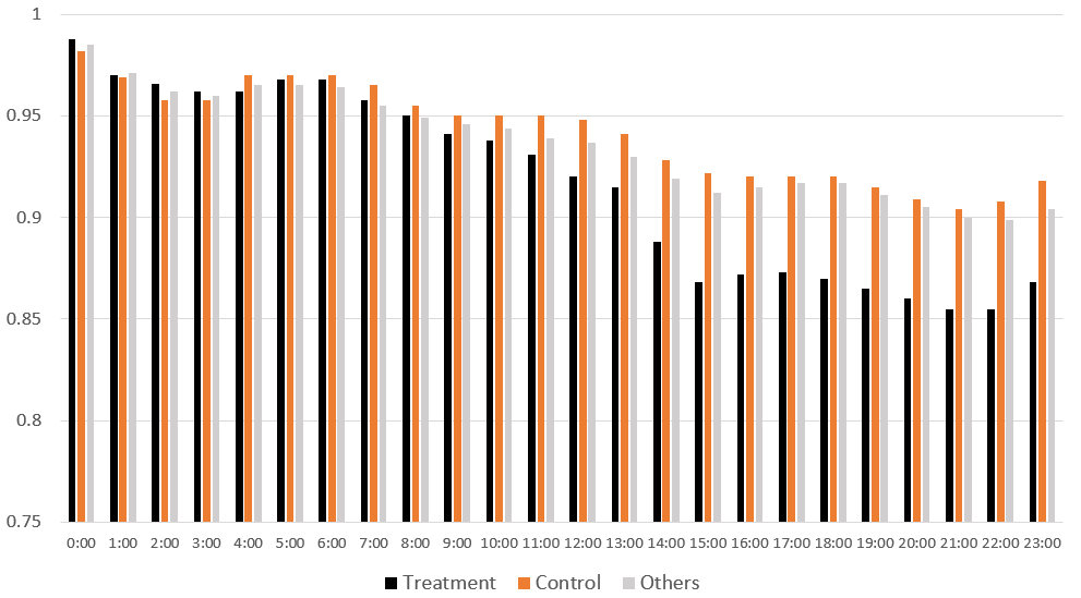
Figure 4: Average $\lambda^{T}$ values, $\bar{\lambda}^{T}$s, for the control ads, treatment ads, and other ads over time in a day.

6 Conclusion

In this paper, we develop a framework to study seller-side experiments affected by interference from feedback loops. Our findings indicate that counterfactual interleaving designs tend to underestimate the true treatment effects when a damping pace algorithm is employed. Additionally, we introduce a method for detecting interference by comparing the rankings of treatment and control groups under the same treatment/control algorithms. As a direction for future research, it would be valuable to explore how experiments can be conducted optimally in scenarios with feedback loops.

Appendix A Proofs

Proof of Proposition 1.

Recall in this case without feedback loops, we have $\Phi^{T}(s,\hat{e})=\Phi^{C}(s,\hat{e})=\hat{e}$. Therefore, we have

$$r_{i}^{GT}(t)=r_{i}^{T}(t)=r_{i}^{C}(t)=r_{i}^{GC}(t),$$

for $i=1,2,\ldots,N$ and $t\in[0,H]$, because of

$$\hat{e}_{i}^{GT}(t)=\hat{e}_{i}^{T}(t)=\hat{e}_{i}^{C}(t)=\hat{e}_{i}^{GC}(t).$$

It further yields

$$I_{i}^{GT}(t)=I_{i}^{T}(t)=I_{i}^{C}(t)=I_{i}^{GC}(t),$$

which means

$$\mathbb{E}\left[\left(\frac{1}{p}\int_{0}^{H}O_{i}^{T}(t)dt\right)\mathbb{I}\{i\in\mathcal{T}\}\right]=\int_{0}^{H}O_{i}^{GT}(t)dt\text{ and}$$

$$\mathbb{E}\left[\left(\frac{1}{1-p}\int_{0}^{H}O_{i}^{T}(t)dt\right)\mathbb{I}\{i\in\mathcal{C}\}\right]=\int_{0}^{H}O_{i}^{GC}(t)dt,$$

for $i=1,2,\ldots,N$. The desired results then follow. ∎

Proof of Proposition 2.

From (24), we know

$$r_{i}^{GT}(t)=r_{i}^{T}(t)\text{ and }r_{i}^{C}(t)=r_{i}^{GC}(t),$$

for $i=1,2,\ldots,N$ and $t\in[0,H]$, given that

$$\hat{e}_{i}^{GT}(t)=\hat{e}_{i}^{T}(t)\text{ and }\hat{e}_{i}^{C}(t)=\hat{e}_{i}^{GC}(t).$$

Then, by comparing (20), (22) with (7) and (21), (23) with (11), we observe

$$I_{i}^{GT}(t)=I_{i}^{T}(t)\text{ and }I_{i}^{C}(t)=I_{i}^{GC}(t).$$

The rest of proof follows the proof of Proposition 1. ∎

Proof of Theorem 1.

We prove the following claim

$$\int_{0}^{t}O_{i}^{E}(s)ds\leq\int_{0}^{t}O_{i}^{GT}(s)ds,\text{ }$$

for $i=1,2,\ldots,N$ and $t\in[0,H]$ by contradiction. Suppose that there exists some $i=$ $1,2,\ldots,N$ and $t\in[0,H]$ such that

$$\int_{0}^{t}O_{i}^{E}(s)ds>\int_{0}^{t}O_{i}^{GT}(s)ds.$$

We first identify when this inequality occurs for the first time:

$$\tau=\inf\left\{t:\text{ there exists }i\text{ such that }\int_{0}^{t}O_{i}^{E}(s)ds>\int_{0}^{t}O_{i}^{GT}(s)ds\right\},$$

and let $\mathcal{I}^{\ast}$ contain the corresponding sellers. That is, for $i^{*}\in\mathcal{I}^{*}$, we have

$$\tau=\inf\left\{t:\int_{0}^{t}O_{i^{*}}^{E}(s)ds>\int_{0}^{t}O_{i^{*}}^{GT}(s)ds\right\},$$ (41)

and for $j\notin\mathcal{I}^{*}$, there exists $t_{0}>\tau$ such that for $t\in[\tau,t_{0}]$,

$$\int_{0}^{t}O_{j}^{E}(s)ds\leq\int_{0}^{t}O_{j}^{GT}(s)ds.$$

By continuity, we have

$$\int_{0}^{\tau}O_{i^{\ast}}^{E}(s)ds=\int_{0}^{\tau}O_{i^{\ast}}^{GT}(s)ds,\text{ for }i^{\ast}\in\mathcal{I}^{\ast},$$ (42)

which implies $S_{i^{*}}^{E}(\tau)=S_{i^{*}}^{GT}(\tau),$ for $i^{\ast}\in\mathcal{I}^{\ast}.$

Due to the inverse monotonocity in Assumption 1.(2), we have

$$r_{i^{\ast}}^{E}(\tau) = r_{i^{\ast}}^{GT}(\tau)\text{ for }i^{\ast}\in\mathcal{I}^{\ast},\text{ }$$ (43)

$$r_{j}^{E}(\tau) \geq r_{j}^{GT}(\tau)\text{ for }j\notin\mathcal{I}^{\ast}.$$ (44)

Then, by Assumption 1.(1), we have

$$f_{i^{\ast}}^{NE}(\tau)$$

$$= f_{i^{\ast}}\left(\left\{r_{j}^{E}(\tau),j=1,2,\ldots,N\right\},\underline{R}(\tau)\right)$$

$$\leq f_{i^{\ast}}\left(\left\{r_{j}^{GT}(\tau),j=1,2,\ldots,N\right\},\underline{R}(\tau)\right)$$

$$= f_{i^{\ast}}^{GT}(\tau).$$

We then consider three different cases.

Case 1: There exists some $i^{\ast}\in\mathcal{I}^{\ast}$ such that

$$f_{i^{\ast}}^{GT}(\tau)>0.$$

By Assumption 3, we have there exists $t_{1}>\tau,$ such that

$$f_{i^{\ast}}^{GT}(t)\geq 0,\text{ for }t\in[\tau,t_{1}]\ ,$$

which means $I_{i^{\ast}}^{GT}(t)=1,$ for $t\in[\tau,t_{1}].$ Then, we have for $t\in[\tau,t_{1}]$

$$\int_{0}^{t}O_{i^{\ast}}^{GT}(s)ds = S_{i^{\ast}}^{GT}(\tau)+\int_{\tau}^{t}e_{i^{\ast}}^{GT}(s)ds$$

$$\geq S_{i^{\ast}}^{E}(\tau)+\int_{\tau}^{t}I_{i^{\ast}}^{E}(s)e_{i^{\ast}}^{E}(s)ds$$

$$= \int_{0}^{t}O_{i^{\ast}}^{E}(s)ds,$$

which contradicts to the definition of $\tau$, as shown in (41).

Case 2: There exists some $i^{\ast}\in\mathcal{I}^{\ast}$ such that

$$0>f_{i^{\ast}}^{NE}(\tau).$$

By Assumption 3, we have there exists $t_{2}>\tau,$ such that

$$f_{i^{\ast}}^{NE}(t)<0,\text{ for }t\in[\tau,t_{2}]\ ,$$

which means $I_{i^{\ast}}^{E}(t)=0,$ for $t\in[\tau,t_{2}].$ Then, we have for $t\in[t,t_{2}]$

$$\int_{0}^{t}O_{i^{\ast}}^{E}(s)ds = S_{i^{\ast}}^{E}(\tau)$$

$$\leq S_{i^{\ast}}^{GT}(\tau)+\int_{\tau}^{t}I_{i^{\ast}}^{GT}(t)e_{i^{\ast}}^{GT}(s)ds$$

$$= \int_{0}^{t}O_{i^{\ast}}^{GT}(s)ds,$$

which contradicts to the definition of $\tau$, as shown in (41).

Case 3: For all $i^{\ast}\in\mathcal{I}^{\ast}$, we have

$$f_{i^{\ast}}^{GT}(\tau)=f_{i^{\ast}}^{NE}(\tau)=0.$$

If $f_{i^{\ast}}^{GT}(t+)>0$, it reduces to the case 1. Similarly, if $f_{i^{\ast}}^{NE}(t+)<0$, it reduces to the case 2. Then, there must exists some $t_{3}\in(\tau,t_{0})$ such that

$$f_{i^{\ast}}^{GT}(t)<0\text{ and }f_{i^{\ast}}^{NE}(t)>0,$$ (45)

for $t\in(\tau,t_{3}]$ and $i^{\ast}\in\mathcal{I}^{\ast}.$ It further yields

$$S_{i^{\ast}}^{E}(t) \geq S_{i^{\ast}}^{GT}(t),\text{ for }i^{\ast}\in\mathcal{I}^{\ast},\text{ }t\in[\tau,t_{3}]\text{ }$$ (46)

$$S_{j}^{E}(t) \leq S_{j}^{GT}(t),\text{ for }j\notin\mathcal{I}^{\ast},\text{ }t\in[\tau,t_{3}].$$ (47)

Due to the inverse monotonocity in Assumption 1.(2), we have

$$r_{i^{\ast}}^{E}(t) \leq r_{i^{\ast}}^{GT}(t)\text{ for }i^{\ast}\in\mathcal{I}^{\ast},\text{ }t\in[\tau,t_{3}]$$ (48)

$$r_{j}^{E}(t) \geq r_{j}^{GT}(t)\text{ for }j\notin\mathcal{I}^{\ast},t\in[\tau,t_{3}].$$ (49)

Then, by Assumption 1.(1), we have for $t\in(\tau,t_{0}],$

$$\sum_{i^{\ast}\in\mathcal{I}^{\ast}}f_{i^{\ast}}^{NE}(t)$$

$$= \sum_{i^{\ast}\in\mathcal{I}^{\ast}}f_{i^{\ast}}\left(\left\{r_{j}^{E}(t),j=1,2,\ldots,N\right\},\underline{R}(t)\right)$$

$$\leq \sum_{i^{\ast}\in\mathcal{I}^{\ast}}f_{i^{\ast}}\left(\left\{r_{i^{\ast}}^{E}(t),i^{\ast}\in\mathcal{I}^{\ast}\right\}\cup\left\{r_{j}^{GT}(t),j\notin\mathcal{I}^{\ast}\right\},\underline{R}(t)\right)$$

$$\leq \sum_{i^{\ast}\in\mathcal{I}^{\ast}}f_{i^{\ast}}\left(\left\{r_{i^{\ast}}^{GT}(t),i^{\ast}\in\mathcal{I}^{\ast}\right\}\cup\left\{r_{j}^{GT}(t),j\notin\mathcal{I}^{\ast}\right\},\underline{R}(t)\right)$$

$$= \sum_{i^{\ast}\in\mathcal{I}^{\ast}}f_{i^{\ast}}^{GT}(t),$$

which contradicts to the inequality (45).

Similarly, we can show

$$\int_{0}^{t}O_{i}^{E}(s)ds\geq\int_{0}^{t}O_{i}^{GC}(s)ds,\text{ }$$

for $i=1,2,\ldots,N$ and $t\in[0,H].$

∎

Proof of Theorem 3.

We proceed in the same manner as the proof of Theorem 1.

We prove the following claim

$$\int_{0}^{t}O_{i}^{E}(s)ds\leq\int_{0}^{t}O_{i}^{GT}(s)ds,\text{ }$$

for $i=1,2,\ldots,N$ and $t\in[0,H]$ by contradiction. Suppose that there exists some $i=$ $1,2,\ldots,N$ and $t\in[0,H]$ such that

$$\int_{0}^{t}O_{i}^{E}(s)ds>\int_{0}^{t}O_{i}^{GT}(s)ds.$$

We first identify when this inequality occurs for the first time:

$$\tau=\inf\left\{t:\text{ there exists some }i\text{ s.t. }\int_{0}^{t}O_{i}^{E}(s)ds>\int_{0}^{t}O_{i}^{GT}(s)ds\right\},$$

and let $\mathcal{I}^{\ast}$ contain the corresponding sellers. By continuity, we have

$$\int_{0}^{\tau}O_{i^{\ast}}^{E}(s)ds=\int_{0}^{\tau}O_{i^{\ast}}^{GT}(s)ds,\text{ for }i^{\ast}\in\mathcal{I}^{\ast}.$$ (50)

Similar to Proof of Theorem 1, we have

$$f_{i^{\ast}}^{CE,T}(\tau)$$

$$= f_{i^{\ast}}\left(\left\{r_{j}^{T}(\tau),j=1,2,\ldots,N\right\},\underline{R}(\tau)\right)$$

$$\leq f_{i^{\ast}}\left(\left\{r_{j}^{GT}(\tau),j=1,2,\ldots,N\right\},\underline{R}(\tau)\right)$$

$$= f_{i^{\ast}}^{GT}(\tau).$$

Cases 1 and 2 are essentially the same as in the proof of Theorem 1.

Case 3: For all $i^{\ast}\in\mathcal{I}^{\ast}$, we have

$$f_{i^{\ast}}^{GT}(\tau) = 0,$$

$$f_{i^{\ast}}^{CE,T}(t) = 0\text{ if }i^{\ast}\in\mathcal{T}\text{ and }f_{i^{\ast}}^{CE,C}(t)=0\text{ if }i^{\ast}\in\mathcal{C}\text{.}$$

There must exists some $t_{3}\in(\tau,t_{0})$ such that

$$f_{i^{\ast}}^{GT}(t) < 0\text{,}$$ (51)

$$f_{i^{\ast}}^{CE,T}(t) > 0\text{ if }i^{\ast}\in\mathcal{T}\text{ and }f_{i^{\ast}}^{CE,C}(t)>0\text{ if }i^{\ast}\in\mathcal{C}\text{, }$$ (52)

for $t\in(\tau,t_{3}]$ and $i^{\ast}\in\mathcal{I}^{\ast}.$

It further yields

$$S_{i^{\ast}}^{E}(t) \geq S_{i^{\ast}}^{GT}(t),\text{ for }i^{\ast}\in\mathcal{I}^{\ast},\text{ }t\in[\tau,t_{3}]\text{ }$$ (53)

$$S_{j}^{E}(t) \leq S_{j}^{GT}(t),\text{ for }j\notin\mathcal{I}^{\ast},\text{ }t\in[\tau,t_{3}].$$ (54)

Due to the inverse monotonocity in Assumption 1.(2), we have

$$r_{i^{\ast}}^{T}(t) \leq r_{i^{\ast}}^{GT}(t)\text{ for }i^{\ast}\in\mathcal{I}^{\ast},\text{ }t\in[\tau,t_{3}]$$ (55)

$$r_{j}^{T}(t) \geq r_{j}^{GT}(t)\text{ for }j\notin\mathcal{I}^{\ast},t\in[\tau,t_{3}].$$ (56)

First, by Assumption 4, we have

$$f_{i^{\ast}}^{CE,C}(t)$$

$$= f_{i^{\ast}}\left(\left\{r_{j}^{C}(t),j=1,2,\ldots,N\right\},\underline{R}(t)\right)$$

$$\leq f_{i^{\ast}}\left(\left\{\alpha r_{j}^{C}(t),j=1,2,\ldots,N\right\},\underline{R}(t)\right)$$

$$= f_{i^{\ast}}\left(\left\{r_{j}^{T}(t),j=1,2,\ldots,N\right\},\underline{R}(t)\right)$$

$$\leq f_{i^{\ast}}^{CE,T}(t).$$

Then, inequalities (51) and (52) imply

$$f_{i^{\ast}}^{GT}(t)<0\text{, }f_{i^{\ast}}^{CE,T}(t)>0\text{, }$$ (57)

for $t\in(\tau,t_{3}]$ and $i^{\ast}\in\mathcal{I}^{\ast}.$

Then, by Assumption 1.(1) and the inequalities (55) and (56), we have for $t\in(\tau,t_{0}],$

$$\sum_{i^{\ast}\in\mathcal{I}^{\ast}}f_{i^{\ast}}^{CE,T}(t)$$

$$= \sum_{i^{\ast}\in\mathcal{I}^{\ast}}f_{i^{\ast}}\left(\left\{r_{j}^{T}(t),j=1,2,\ldots,N\right\},\underline{R}(t)\right)$$

$$\leq \sum_{i^{\ast}\in\mathcal{I}^{\ast}}f_{i^{\ast}}\left(\left\{r_{i^{\ast}}^{T}(t),i^{\ast}\in\mathcal{I}^{\ast}\right\}\cup\left\{r_{j}^{GT}(t),j\notin\mathcal{I}^{\ast}\right\},\underline{R}(t)\right)$$

$$\leq \sum_{i^{\ast}\in\mathcal{I}^{\ast}}f_{i^{\ast}}\left(\left\{r_{i^{\ast}}^{GT}(t),i^{\ast}\in\mathcal{I}^{\ast}\right\}\cup\left\{r_{j}^{GT}(t),j\notin\mathcal{I}^{\ast}\right\},\underline{R}(t)\right)$$

$$= \sum_{i^{\ast}\in\mathcal{I}^{\ast}}f_{i^{\ast}}^{GT}(t),$$

which contradicts to the inequalities (57). ∎

References

- (1)
- Aronow and Samii (2013) Peter M Aronow and Cyrus Samii. 2013. Estimating Average Causal Effects Under General Interference, with Application to a Social Network Experiment. arXiv preprint arXiv:1305.6156 (2013).
- Bajari et al. (2021) Patrick Bajari, Brian Burdick, Guido W Imbens, Lorenzo Masoero, James McQueen, Thomas Richardson, and Ido M Rosen. 2021. Multiple randomization designs. arXiv preprint arXiv:2112.13495 (2021).
- Basse et al. (2023) Guillaume W Basse, Yi Ding, and Panos Toulis. 2023. Minimax designs for causal effects in temporal experiments with treatment habituation. Biometrika 110, 1 (2023), 155–168.
- Blake and Coey (2014) Thomas Blake and Dominic Coey. 2014. Why marketplace experimentation is harder than it seems: The role of test-control interference. In Proceedings of the fifteenth ACM conference on Economics and computation. 567–582.
- Bojinov et al. (2023) Iavor Bojinov, David Simchi-Levi, and Jinglong Zhao. 2023. Design and analysis of switchback experiments. Management Science 69, 7 (2023), 3759–3777.
- Bright et al. (2022) Ido Bright, Arthur Delarue, and Ilan Lobel. 2022. Reducing marketplace interference bias via shadow prices. arXiv preprint arXiv:2205.02274 (2022).
- Candogan et al. (2023) Ozan Candogan, Chen Chen, and Rad Niazadeh. 2023. Correlated cluster-based randomized experiments: Robust variance minimization. Management Science (2023).
- Chaney et al. (2018) Allison JB Chaney, Brandon M Stewart, and Barbara E Engelhardt. 2018. How algorithmic confounding in recommendation systems increases homogeneity and decreases utility. In Proceedings of the 12th ACM conference on recommender systems. 224–232.
- Eckles et al. (2017) Dean Eckles, Brian Karrer, and Johan Ugander. 2017. Design and analysis of experiments in networks: Reducing bias from interference. Journal of Causal Inference 5, 1 (2017).
- Fan et al. (2022) Yewen Fan, Nian Si, and Kun Zhang. 2022. Calibration Matters: Tackling Maximization Bias in Large-scale Advertising Recommendation Systems. arXiv preprint arXiv:2205.09809 (2022).
- Farias et al. (2022) Vivek Farias, Andrew Li, Tianyi Peng, and Andrew Zheng. 2022. Markovian interference in experiments. Advances in Neural Information Processing Systems 35 (2022), 535–549.
- Farias et al. (2023) Vivek Farias, Hao Li, Tianyi Peng, Xinyuyang Ren, Huawei Zhang, and Andrew Zheng. 2023. Correcting for Interference in Experiments: A Case Study at Douyin. In Proceedings of the 17th ACM Conference on Recommender Systems. 455–466.
- Fradkin (2015) Andrey Fradkin. 2015. Search frictions and the design of online marketplaces. In The Third Conference on Auctions, Market Mechanisms and Their Applications.
- Glynn et al. (2020) Peter W Glynn, Ramesh Johari, and Mohammad Rasouli. 2020. Adaptive experimental design with temporal interference: A maximum likelihood approach. Advances in Neural Information Processing Systems 33 (2020), 15054–15064.
- Goli et al. (2023) Ali Goli, Anja Lambrecht, and Hema Yoganarasimhan. 2023. A bias correction approach for interference in ranking experiments. Marketing Science (2023).
- Gui et al. (2015) Huan Gui, Ya Xu, Anmol Bhasin, and Jiawei Han. 2015. Network a/b testing: From sampling to estimation. In Proceedings of the 24th International Conference on World Wide Web. 399–409.
- Guo et al. (2023) Hongbo Guo, Ruben Naeff, Alex Nikulkov, and Zheqing Zhu. 2023. Evaluating Online Bandit Exploration In Large-Scale Recommender System. In KDD-23 Workshop on Multi-Armed Bandits and Reinforcement Learning: Advancing Decision Making in E-Commerce and Beyond.
- Ha-Thuc et al. (2020) Viet Ha-Thuc, Avishek Dutta, Ren Mao, Matthew Wood, and Yunli Liu. 2020. A counterfactual framework for seller-side a/b testing on marketplaces. In Proceedings of the 43rd International ACM SIGIR Conference on Research and Development in Information Retrieval. 2288–2296.
- Harshaw et al. (2023) Christopher Harshaw, Fredrik Sävje, David Eisenstat, Vahab Mirrokni, and Jean Pouget-Abadie. 2023. Design and analysis of bipartite experiments under a linear exposure-response model. Electronic Journal of Statistics 17, 1 (2023), 464–518.
- Holtz and Aral (2020) David Holtz and Sinan Aral. 2020. Limiting bias from test-control interference in online marketplace experiments. arXiv preprint arXiv:2004.12162 (2020).
- Holtz et al. (2023) David Holtz, Jennifer Brennan, and Jean Pouget-Abadie. 2023. A Study of” Symbiosis Bias” in A/B Tests of Recommendation Algorithms. arXiv preprint arXiv:2309.07107 (2023).
- Holtz et al. (2020) David Holtz, Ruben Lobel, Inessa Liskovich, and Sinan Aral. 2020. Reducing interference bias in online marketplace pricing experiments. arXiv preprint arXiv:2004.12489 (2020).
- Hu and Wager (2022) Yuchen Hu and Stefan Wager. 2022. Switchback experiments under geometric mixing. arXiv preprint arXiv:2209.00197 (2022).
- Hudgens and Halloran (2008) Michael G Hudgens and M Elizabeth Halloran. 2008. Toward causal inference with interference. J. Amer. Statist. Assoc. 103, 482 (2008), 832–842.
- Imbens and Rubin (2015) Guido W Imbens and Donald B Rubin. 2015. Causal inference in statistics, social, and biomedical sciences. Cambridge University Press.
- Jadidinejad et al. (2020) Amir H Jadidinejad, Craig Macdonald, and Iadh Ounis. 2020. Using exploration to alleviate closed loop effects in recommender systems. In Proceedings of the 43rd International ACM SIGIR Conference on Research and Development in Information Retrieval. 2025–2028.
- Johari et al. (2022) Ramesh Johari, Hannah Li, Inessa Liskovich, and Gabriel Y Weintraub. 2022. Experimental design in two-sided platforms: An analysis of bias. Management Science (2022).
- Karlsson (2020) Niklas Karlsson. 2020. Feedback control in programmatic advertising: The frontier of optimization in real-time bidding. IEEE Control Systems Magazine 40, 5 (2020), 40–77.
- Khenissi (2022) Sami Khenissi. 2022. Modeling and debiasing feedback loops in collaborative filtering recommender systems. (2022).
- Krauth et al. (2022) Karl Krauth, Yixin Wang, and Michael I Jordan. 2022. Breaking feedback loops in recommender systems with causal inference. arXiv preprint arXiv:2207.01616 (2022).
- Li et al. (2023) Shuangning Li, Ramesh Johari, Stefan Wager, and Kuang Xu. 2023. Experimenting under Stochastic Congestion. arXiv preprint arXiv:2302.12093 (2023).
- Li and Wager (2022) Shuangning Li and Stefan Wager. 2022. Random graph asymptotics for treatment effect estimation under network interference. The Annals of Statistics 50, 4 (2022), 2334–2358.
- Liu et al. (2021) Min Liu, Jialiang Mao, and Kang Kang. 2021. Trustworthy and powerful online marketplace experimentation with budget-split design. In Proceedings of the 27th ACM SIGKDD Conference on Knowledge Discovery & Data Mining. 3319–3329.
- Mansoury et al. (2020) Masoud Mansoury, Himan Abdollahpouri, Mykola Pechenizkiy, Bamshad Mobasher, and Robin Burke. 2020. Feedback loop and bias amplification in recommender systems. In Proceedings of the 29th ACM international conference on information & knowledge management. 2145–2148.
- Musgrave et al. (2023) Paul Musgrave, Cuize Han, and Parth Gupta. 2023. Measuring service-level learning effects in search via query-randomized experiments. (2023).
- Nandy et al. (2021) Preetam Nandy, Divya Venugopalan, Chun Lo, and Shaunak Chatterjee. 2021. A/b testing for recommender systems in a two-sided marketplace. Advances in Neural Information Processing Systems 34 (2021), 6466–6477.
- Ni et al. (2023) Tu Ni, Iavor Bojinov, and Jinglong Zhao. 2023. Design of Panel Experiments with Spatial and Temporal Interference. Available at SSRN 4466598 (2023).
- Pan et al. (2021) Weishen Pan, Sen Cui, Hongyi Wen, Kun Chen, Changshui Zhang, and Fei Wang. 2021. Correcting the user feedback-loop bias for recommendation systems. arXiv preprint arXiv:2109.06037 (2021).
- Pearl (2000) Judea Pearl. 2000. Causality: Models, reasoning and inference. Cambridge, UK: CambridgeUniversityPress 19, 2 (2000), 3.
- Pouget-Abadie et al. (2019) Jean Pouget-Abadie, Kevin Aydin, Warren Schudy, Kay Brodersen, and Vahab Mirrokni. 2019. Variance reduction in bipartite experiments through correlation clustering. Advances in Neural Information Processing Systems 32 (2019).
- Si (2023) Nian Si. 2023. Tackling Interference Induced by Data Training Loops in A/B Tests: A Weighted Training Approach. arXiv preprint arXiv:2310.17496 (2023).
- Si et al. (2022) Nian Si, San Gultekin, Jose Blanchet, and Aaron Flores. 2022. Optimal Bidding and Experimentation for Multi-Layer Auctions in Online Advertising. Available at SSRN (2022). https://papers.ssrn.com/sol3/papers.cfm?abstract_id=4358914
- Ugander et al. (2013) Johan Ugander, Brian Karrer, Lars Backstrom, and Jon Kleinberg. 2013. Graph cluster randomization: Network exposure to multiple universes. In Proceedings of the 19th ACM SIGKDD international conference on Knowledge discovery and data mining. 329–337.
- Ugander and Yin (2023) Johan Ugander and Hao Yin. 2023. Randomized graph cluster randomization. Journal of Causal Inference 11, 1 (2023), 20220014.
- Wang and Ba (2023) Yan Wang and Shan Ba. 2023. Producer-Side Experiments Based on Counterfactual Interleaving Designs for Online Recommender Systems. arXiv preprint arXiv:2310.16294 (2023).
- Xiong et al. (2019) Ruoxuan Xiong, Susan Athey, Mohsen Bayati, and Guido Imbens. 2019. Optimal experimental design for staggered rollouts. arXiv preprint arXiv:1911.03764 (2019).
- Xiong et al. (2023b) Ruoxuan Xiong, Alex Chin, Mohsen Bayati, and Sean Taylor. 2023b. Data-Driven Switchback Design. preprint (2023). https://www.ruoxuanxiong.com/data-driven-switchback-design.pdf
- Xiong et al. (2023a) Ruoxuan Xiong, Alex Chin, and Sean Taylor. 2023a. Bias-variance tradeoffs for designing simultaneous temporal experiments. In The KDD’23 Workshop on Causal Discovery, Prediction and Decision. PMLR, 115–131.
- Yang et al. (2023) Mengyue Yang, Jun Wang, and Jean-Francois Ton. 2023. Rectifying unfairness in recommendation feedback loop. In Proceedings of the 46th international ACM SIGIR Conference on Research and Development in Information Retrieval. 28–37.
- Ye et al. (2023) Zikun Ye, Dennis J Zhang, Heng Zhang, Renyu Zhang, Xin Chen, and Zhiwei Xu. 2023. Cold start to improve market thickness on online advertising platforms: Data-driven algorithms and field experiments. Management Science 69, 7 (2023), 3838–3860.
- Yu et al. (2022) Christina Lee Yu, Edoardo M Airoldi, Christian Borgs, and Jennifer T Chayes. 2022. Estimating the total treatment effect in randomized experiments with unknown network structure. Proceedings of the National Academy of Sciences 119, 44 (2022), e2208975119.