On the discrete Dirac spectrum of general-relativistic hydrogenic ions with anomalous magnetic moment

Abstract

The Reissner–Weyl–Nordström (RWN) spacetime of a point nucleus features a naked singularity for the empirically known nuclear charges $Ze$ and masses $M=A(Z,N)m_{\mathrm{p}}$, where $m_{\mathrm{p}}$ is the proton mass and $A(Z,N)\approx Z+N$ the atomic mass number, with $Z$ the number of protons and $N$ the number of neutrons in the nucleus. The Dirac hamiltonian for a test electron with mass $m_{\mathrm{e}}$, charge $-e$, and anomalous magnetic moment $\mu_{a}(\approx-\frac{1}{4\pi}\frac{e^{3}}{m_{\mathrm{e}}c^{2}})$ in the electrostatic RWN spacetime of such a ‘naked point nucleus’ is known to be essentially self-adjoint, with a spectrum that consists of the union of the essential spectrum $(-\infty,-m_{\mathrm{e}}c^{2}]\cup[m_{\mathrm{e}}c^{2},\infty)$ and a discrete spectrum of infinitely many eigenvalues in the gap $(-m_{\mathrm{e}}c^{2},m_{\mathrm{e}}c^{2})$, having $m_{\mathrm{e}}c^{2}$ as accumulation point. In this paper the discrete spectrum is characterized in detail for the first time, for all $Z\leq 45$ and $A$ that cover all known isotopes. The eigenvalues are mapped one-to-one to those of the traditional Dirac Hydrogen spectrum. Numerical evaluations that go beyond $Z=45$ into the realm of not-yet-produced hydrogenic ions are presented, too. A list of challenging open problems concludes this publication.

 

©The authors. Reproduction, in its entirety, is permitted for non-commercial purposes.

1 Introduction

One of the fundamental axioms of quantum theory stipulates that the quantum state of an isolated system evolves unitarily. By Stone’s theorem a unitary time evolution is generated by a unique self-adjoint operator. In quantum mechanics this operator is known as the hamiltonian of the system. The formal expressions for such Hamilton operators as suggested by some basic physical reasoning are rarely a priori self-adjoint, though. Instead they are only symmetric on some convenient but often too small a domain. In the absence of a universally accepted principle that would dictate which self-adjoint extension would capture the physics correctly, physicists face the conceptual conundrum of having to decide this question case by case — assuming here that a self-adjoint extension exists in each case.

In the following we discuss this fundamental conceptual issue by focusing on hydrogenic ions. Since the theory of hydrogenic ions has been such an important stepping stone in the development of quantum mechanics, it may be surprising to learn that the problem of choosing the physically correct self-adjoint hamiltonian is far from being completely settled and understood. Our main novel mathematical contribution in this paper, as summarized in the abstract, is meant as one small further step on the way to settle the hydogenic problem for good. Those readers familiar with this intriguing background story may now want to skip directly to section 1.3.1 for the informal statement of our main result, and then move on to the technical sections of our paper. Everyone else is invited to read the rest of this introduction and be intrigued by the unfolding story.

Throughout we will be concerned exclusively with the quantum-mechanical problem of a single point electron in the electrostatic spacetime — which can be flat or curved — of a fixed point nucleus. Thus we only treat the electron degrees of freedom quantum-mechanically. The nucleus has charge $Q=Ze$, where $e>0$ denotes the elementary charge (in Gaussian units), and $Z\in\mathbb{N}$ counts the number of elementary charges carried by the nucleus. The nuclear ADM mass $M_{\mbox{\tiny{ADM}}}=M>0$; in particular, the proton mass is denoted $m_{\mathrm{p}}$. Moreover, $m_{\mathrm{e}}$ is the empirical mass of the electron, and $-e$ its charge; we shall also consider the anti-electron (positron), having charge $+e$ and mass $m_{\mathrm{e}}$. Beside these particle parameters, Newton’s constant of universal gravitation $G$, the speed of light in vacuum $c$, and $\hbar$, Planck’s constant divided by $2\pi$, will appear in our formulas.

1.1 The non-relativistic problem

Consider first the non-relativistic problem, with the Schrödinger hamiltonian

$$H=-\frac{\hbar^{2}}{2m_{\mathrm{e}}}\Delta-(Ze^{2}+GMm_{\mathrm{e}})\frac{1}{r},$$ (1.1)

acting classically and automorphically on complex-valued functions $\psi\in D_{\rm min}(H)=C^{\infty}_{c}(\mathbb{R}^{3}\backslash\{0\})\subset L^{2}(\mathbb{R}^{3})$. After a decomposition of the operator (1.1) into its partial wave operators that act on the invariant subspaces indexed by the angular momentum eigenvalues $\ell\in\{0,1,2,...\}$, an application of Weyl’s limit point / limit circle criterion (see [39]) reveals that the radial $\ell=0$ operators are not essentially self-adjoint on their minimal domain $C^{\infty}_{c}(\mathbb{R}_{+}\backslash\{0\})$, but that there exists a continuously parameterized family of self-adjoint extensions; see Thm.X.11 in [31]. Their spectra [2], [1] generally differ from the textbook Bohr spectrum, except for one special parameter value when the self-adjoint extension agrees with the Friedrichs extension that is used by physicists. Without the availability of empirical Hydrogen spectral data, the non-relativistic Schrödinger operator on $C^{\infty}_{c}(\mathbb{R}^{3}\backslash\{0\})$ would not in itself be able to suggest the self-adjoint extension that would capture the physical empiricism correctly.

The continuous family of self-adjoint extensions of (1.1) invokes some “boundary condition” on the Schrödinger wave function $\psi$ at $r=0$. One might want to argue that the theory that reproduces the correct physical spectral data for hydrogenic ions should not depend on such fine details like boundary conditions at the point nucleus. After all, the fiction of a point nucleus has been chosen for mathematical convenience precisely for the same reason: the typical distance between proton and electron in the Hydrogen ground state is about $10^{5}$ times larger than the empirical size of the proton, so that the details of the structure of the proton — and, by analogy, of the nucleus of a hydrogenic ion (at least if not too massive) — should be irrelevant for the determination of the main spectral structure. In essence this seems to have been the line of reasoning of Tosio Kato, who in the late 1940s showed [22] that the Hamilton operator (1.1) is essentially self-adjoint when defined on the dense domain $C^{\infty}_{c}(\mathbb{R}^{3})\subset L^{2}(\mathbb{R}^{3})$. Its unique self-adjoint extension agrees with the Friedrichs extension that corresponds to the energy functional conventionally employed by physicists, and its discrete spectrum is identical to the Bohr spectrum, as is well known.

Incidentally, everything we wrote about essential self-adjointness for (1.1) applies equally well when both Coulomb electricity and Newton gravity are taken into account, as featured explicitly in (1.1), or when only one but not the other of these interactions is considered. The spectrum of the Friedrichs extension of (1.1) can be explicitly computed (as done first by Schrödinger himself [34]), revealing that the discrete spectrum consists of the eigenvalues

$$E_{n}^{\rm Bohr}=-\frac{1}{2}\frac{(Ze^{2}+GMm_{\mathrm{e}})^{2}m_{\mathrm{e}}}{\hbar^{2}}\frac{1}{n^{2}}$$ (1.2)

with $n\in\mathbb{N}$. Now recall that $\frac{GMm_{\mathrm{e}}}{Ze^{2}}\approx 10^{-40}$. This quantitative estimate is usually invoked in elementary atomic physics textbooks in arguments for why the influence of atomic gravity on the atomic spectra is immeasurably small for all practical purposes, and thus negligible.

The practical success of Kato’s reasoning would seem to suggest that the principle that guides the quest for the physically correct hamiltonian is to choose the largest possible one of all the self-adjoint extensions. While one cannot argue with success, as the saying goes, one has to swallow this principle of the maximal domain of self-adjointness with a grain of salt. Indeed, while it is plausible, it is not compelling, and is vindicated only by its practical success. For those physicists who adhere too literally to the characterization of physics as an experimental science, this empirical success may be all that matters. Our paper is motivated by the conviction that mathematically logical coherence of a physical theory is an equally important ingredient to assess the merits of a physical theory.

In this vein, a manifestly more conceptually compelling principle is the following.

1.2 The special-relativistic problem

Schrödinger’s operator (1.1) is only thought to be a non-relativistic approximation to a putatively more fundamental relativistic operator. Considering first only special relativity, the operator in question is the Dirac operator of hydrogenic ions,

$$H=-i\hbar c\vec{\boldsymbol{\alpha}}\cdot\nabla+m_{\mathrm{e}}c^{2}\boldsymbol{\beta}-Ze^{2}\frac{1}{r}\boldsymbol{1}$$ (1.3)

acting on four-component complex bi-spinor wave functions $\Psi$ on the minimal domain $\big{(}C^{\infty}_{c}(\mathbb{R}^{3}\backslash\{0\})\big{)}^{4}\subset\big{(}L^{2}(\mathbb{R}^{3})\big{)}^{4}$. As shown first by Weidmann [39], this special-relativistic Dirac hamiltonian for hydrogenic ions with purely electrical Coulomb interactions is essentially self-adjoint on $\big{(}C^{\infty}_{c}(\mathbb{R}^{3}\backslash\{0\})\big{)}^{4}$ for $Z\leq 118$; cf. [35]. This covers all empirically known nuclei, which includes not only those that occur in nature ($Z\leq 92$) but also all those produced artificially in nuclear reactors or heavy ion collisions.

Thus, the Dirac hamiltonian (1.3), defined on its minimal domain, has a unique self-adjoint extension when $Z\leq 118$. Moreover, as shown first by Darwin [10] and Gordon [16], and reproduced many times since with various techniques (cf. [36], [17]), its spectrum can be computed in closed form. In particular, the discrete spectrum reproduces the Sommerfeld fine structure formula, i.e. for $n\in\mathbb{N}$ and $k\in\{-n,\dots,-1,1,\dots,n-1\}$ one has

$$E_{n,k}^{\rm Dirac}=\frac{m_{\mathrm{e}}c^{2}}{\sqrt{1+\frac{Z^{2}\alpha_{\mbox{\tiny{S}}}^{2}}{\left(n-|k|+\sqrt{k^{2}-Z^{2}\alpha_{\mbox{\tiny{S}}}^{2}}\right)^{2}}}},$$ (1.4)

where

$$\alpha_{\mbox{\tiny{S}}}\,=\,\frac{e^{2}}{\hbar c}\approx\frac{1}{137.036}$$ (1.5)

is Sommerfeld’s fine structure constant. Armed with these explicit formulas it is straightforward to take the non-relativistic limit (formally letting the speed of light $c\to\infty$; for a technically careful procedure see [36]). One finds that the discrete spectrum (after first subtracting $m_{\mathrm{e}}c^{2}$) converges to the Bohr spectrum of the Friedrichs extension of the hydrogenic Schrödinger Hamilton operator. The suggestive conclusion is that relativity theory takes care of the theoretical self-adjointness ambiguity that exists at the non-relativistic level of Schrödinger theory. Indeed, it stands to reason that the non-relativistic limit of an essentially self-adjoint hydrogenic Dirac hamiltonian with $Z\leq 118$ yields a more compelling selection principle for the hydrogenic hamiltonian at the non-relativistic level than the practical success of Kato’s maximal self-adjoint extension principle.

But what about the regime $Z>118$? And what about gravity? We now address these two issues one by one, beginning with the special-relativistic large $Z$ regime.

Since empirically $Z\leq 118$ so far, one may not be too alarmed about the lack of essential self-adjointness of the special-relativistic Dirac operator for hydrogenic ions with $Z>118$. Be that as it may, physicists for quite some time already have been trying to create super-heavy ions with $Z>118$ using heavy ion collisions, in the expectation of finding some novel states of nuclear matter, and to gain some theoretical insights they have continued to use the special-relativistic Dirac operator for hydrogenic ions with point nuclei; cf. [17]. Precisely because there are no empirical data yet that could guide one’s choice, this regime is perfectly suited to illustrate the dilemma one faces when essential self-adjointness fails.

Thus, when $119\leq Z\leq 137$, the Dirac operator (1.3) defined on its minimal domain does have a distinguished self-adjoint extension, defined by allowing $Z\in\mathbb{C}$ and demanding analyticity in $Z$ in the neighborhood of $Z=0$ for its self-adjoint extension, as shown by Narnhofer [26]. The Dirac operator (1.3) defined on its minimal domain is then essentially self-adjoint for $Z\leq\sqrt{3}/2\alpha_{\mbox{\tiny{S}}}(\approx 118.677)$, and has a self-adjoint extension that depends on $Z$ analytically for all $Z\in(0,1/\alpha_{\mbox{\tiny{S}}})$, with $1/\alpha_{\mbox{\tiny{S}}}\approx 137.036$. Yet, is analyticity a compelling distinction? Recall that in thermodynamics the important phenomenon of a phase transition is associated with precisely such a point of non-analyticity for the pertinent thermodynamic potential. Thus, is $Z=118$, or more accurately $Z=\frac{1}{2}\sqrt{3}$, perhaps the hydrogenic spectral analog of a point of phase transition beyond which analyticity fails to predict the correct self-adjoint extension? We believe it’s fair to suspect that nobody knows.

As pointed out in [17], this analytic extension is also the only one for which all bound states do have finite quantum expected values separately for kinetic and for potential energy. This is an interesting observation, through which the analytic self-adjoint extension is doubly distinguished, but is this a compelling principle to select this self-adjoint extension? And even if one supposes that for the theory of atomic spectra the principle of analyticity rules supreme, or the principle that kinetic and potential energy expected values have to be finite separately, it only gets one to $Z=137$.

A compelling way out of the dilemma was noted first by Behncke [6], and amplified subsequently by Arnold–Kalf–Schneider [3] and by Gesztezy–Simon–Thaller [15] (see also [36]). These authors pointed out that the problem of the lack of essential self-adjointness of (1.3) for when $Z>118$ goes away if one takes the anomalous magnetic moment $\mu_{a}$ of the electron into account. This means to replace (1.3) by

$$H=-i\hbar c\vec{\boldsymbol{\alpha}}\cdot\nabla+m_{\mathrm{e}}c^{2}\boldsymbol{\beta}-Ze^{2}\frac{1}{r}\boldsymbol{1}+i\mu_{a}Ze\boldsymbol{\beta}\vec{\boldsymbol{\alpha}}\cdot\nabla\frac{1}{r},$$ (1.6)

with $\mu_{a}<0$ [14]. The operator (1.6) on its minimal domain is essentially self-adjoint for all $Z>0$. This would seem to be a weighty argument for its physical significance, except for the following caveat: The anomalous magnetic moment of the electron is conventionally explained as a quantum-electrodynamical effect, and it is somewhat unsatisfactory if a non-rigorous perturbative quantum field-theoretical calculation [9] is invoked to rescue quantum mechanics from one of its conceptual dilemmas.

But now consider this: In magnitude, the leading order contribution to the anomalous magnetic moment of the electron, according to QED’s expansion in powers of Sommerfeld’s $\alpha_{\mbox{\tiny{S}}}$ and its logarithm, is the product of the Bohr magneton $\mu_{\mbox{\tiny{B}}}=\frac{1}{4\pi}\frac{he}{m_{\mathrm{e}}c}$ and the factor $\frac{1}{2\pi}\alpha_{\mbox{\tiny{S}}}$, with $\alpha_{\mbox{\tiny{S}}}$ given in (1.5). More to the point, the anomalous magnetic moment in highly accurate approximation reads $\mu_{a}\approx-\mu_{\rm cl}$, with

$$\mu_{\rm cl}:=\frac{1}{4\pi}\frac{e^{3}}{m_{\mathrm{e}}c^{2}},$$ (1.7)

which is independent of $\hbar$, and in this sense is a classical physics quantity, named the classical magnetic moment of the electron in [25]. Therefore the Dirac operator (1.6) can be viewed as obtained by quantizing a classical special-relativistic theory of an electron with charge $-e$ and anomalous magnetic moment of magnitude $\mu_{\rm cl}$, as expected for a properly quantum-mechanical theory of hydrogenic ions. This removes the caveat expressed above.

Having convincingly overcome the self-adjointness problem for this special-relativistic model of hydrogentic ions with point nuclei, the next question is whether the spectrum of (1.6) is compatible with empirical data. Since so far we do not have any data for $Z>118$, for now this viability question can only be decided by comparing the spectrum of (1.6) with data for when $Z\leq 118$. We don’t attempt to do this here, but emphasize that in principle it is a well-defined problem.

On the theoretical side the following contributions towards answering the above viability question have so far been made:

An important analytical result has been contributed by Kalf and Schmidt [21], and completed by Schmidt [33]. They noted that when $Z\leq 118$ (or rather $Z\leq\frac{\sqrt{3}}{2}\frac{1}{\alpha_{\mbox{\tiny{S}}}}$), then (1.6) converges in strong resolvent sense to (1.3) in the limit $\mu_{a}\to 0$. This alone does not imply convergence of the point spectra. They then went on to prove that when $Z\leq 137$ (or rather $Z<\frac{1}{\alpha_{\mbox{\tiny{S}}}}$), then the eigenvalues of the unique self-adjoint operator with anomalous magnetic moment converge to those of the distinguished self-adjoint extension of the one without. Thus, if $|\mu_{a}|$ is small enough, then the spectral results will differ only ever so slightly.

But how small is “small enough”? In particular, what about spectral results for the physical $\mu_{a}$ given in (1.7)? In the physics literature one traditionally finds non-rigorous perturbative treatments; cf. [9]. A non-perturbative numerical evaluation of a handful of low-lying eigenvalues has been carried out by the Thallers, see [36] (section 7, and the dedication) and [37], though unfortunately without revealing the details of how the numerical evaluation has been accomplished. Numerically they compared the electron’s lowest eigenvalue of (1.3) with that of (1.6). Their eigenvalue plot (see Fig. 7.1 in [36]) suggests that these lowest eigenvalues must be barely distinguishable for all naturally occurring $Z$, while significant discrepancies become visible when $Z>118$; the lowest eigenvalue of (1.3) terminates when $Z\nearrow 137.036$, while its counterpart for (1.6) continues to exist until it meets the previously second-lowest eigenvalue at about $Z\approx 145$ with value $E\approx 0$. There a cross-over happens, and both eigenvalues continue to decrease until they meet the negative continuum roughly when $Z\approx 147$, resp. $Z\approx 160$. We have not seen any confirmation of these numerical results by other authors. This is one of the open issues that we address in our paper, as the special-relativistic limit of our main inquiry.

1.3 The general-relativistic problem

While one may be inclined to dismiss the $Z>118$ problem as of rather academical interest, gravity certainly acts between the electron and the nucleus in all known hydrogenic ions, and although the non-relativistic estimates suggest that gravity makes practically immeasurably small contributions only, conceptually it is mandatory to include this force of nature in the model. Its absence from the special-relativistic Dirac operator for hydrogenic ions means that the essential self-adjointness of the latter for $Z\leq 118$ (in the absence of the $\mu_{a}$ term) vindicates only the Friedrichs extension of the Schrödinger operator (1.1) (that does not feature $\mu_{a}$) with electrical Coulomb but no gravitational Newton interactions (for $Z\leq 118$, although for $Z$ that large the Schrödinger operator is not capturing the physics accurately any longer). To address this deficiency in a conceptually principled manner one has to start from the general-relativistic Dirac operator of hydrogenic ions.

The direct general-relativistic counterpart to both, Schrödinger’s (1.1) and Dirac’s (1.3), is the Dirac hamiltonian extracted from Dirac’s equation for a point electron in the Reissner–Weyl–Nordström (RWN) spacetime of a point nucleus.

The RWN spacetime [41], [32], [27] is a static, spherically symmetric Lorentzian manifold with two real parameters: the ADM mass $M\geq 0$ and charge $Q$; for hydrogenic ions, $Q=Ze>0$. Using the $(+,-,-,-)$ signature, the line element corresponding to the Lorentzian metric is

$$ds^{2}\,=\,f(r)^{2}c^{2}dt^{2}-\frac{1}{f(r)^{2}}dr^{2}-r^{2}d\Omega^{2},$$ (1.8)

where $d\Omega^{2}$ is the usual round metric on $\mathbb{S}^{2}$ and

$$f(r)^{2}\,=\,{1-\frac{G}{c^{2}}\,\frac{2M}{r}+\frac{G}{c^{4}}\,\frac{Z^{2}e^{2}}{r^{2}}}\,.$$ (1.9)

All known nuclei are in the naked singularity sector, $GM^{2}<Z^{2}e^{2}$; in fact, we have $GM^{2}\ll Z^{2}e^{2}$ by more than thirty orders of magnitude. In this case, $f(r)^{2}$ is strictly positive for all $r>0$, and we stipulate $f(r)$ to be its positive square root. There is a curvature singularity at $r=0$; consequently, the maximally extended analytic manifold is ${{\mathcal{M}}}=\mathbb{R}\times(0,\infty)\times\mathbb{S}^{2}$.

The Dirac equation for a point electron in the RWN spacetime reads

$$\tilde{\gamma}^{\mu}(i\hbar c\nabla_{\mu}-eA_{\mu})\Psi-m_{\mathrm{e}}c^{2}\Psi\,=\,0.$$ (1.10)

Here, $\Psi\colon{{\mathcal{M}}}\to\mathbb{C}^{4}$ is a bi-spinor field on the spacetime manifold, $\nabla_{\mu}$ is the covariant derivative acting on bi-spinors, and $\tilde{\gamma}^{\mu}$ are the Dirac matrices that satisfy the anti-commutation relations with respect to the Lorentzian metric (1.8), (1.9). The Dirac matrices generate the complexified Clifford algebra $\text{Cl}_{1,3}(\mathbb{R})_{\mathbb{C}}$ over each tangent space $T_{p}{{\mathcal{M}}}$ on the manifold. Finally, $A=-\frac{Q}{r}cdt$ is the one-form of the electromagnetic potential of the RWN spacetime, which is purely electrostatic. In the $(x^{0}=ct,r,\theta,\phi)$ coordinates, the only nonzero component of $A$ is $A_{0}=-\frac{Q}{r}$. The quantum-mechanical Dirac operator $H$ is now extracted from (1.10) by rewriting this Dirac equation into the abstract Schrödinger format $i\hbar\partial_{t}\Psi=H\Psi$.

It came as a big surprise when in 1982 Cohen and Powers [8] proved that this general-relativistic Dirac operator for hydrogenic ions is not essentially self-adjoint on its minimal domain but has a continuously parameterized family of self-adjoint extensions, each one (presumably) with its own discrete spectrum. It seems that general relativity throws us back to the same self-adjointness ambiguity that plagues the non-relativistic Schrödinger problem (1.1). Worse, since the Dirac operator is unbounded above and below, one now cannot invoke a Friedrichs extension as a putatively distinguished self-adjoint extension. Einstein’s gravity clearly is not a weak perturbation of Coulomb electricity in the sense that Newton’s gravity is — it has devastating effects on the quantum-mechanical theory of all the hydrogenic spectra, Hydrogen itself included.

About 20 years later, Belgiorno, Martinelli, and Baldicchi [7] showed that the replacement of (1.10) with the Dirac equation that includes a term for the electron’s anomalous magnetic moment coupled to the gradient of the Coulomb field (see next section) restores essential self-adjointness — though only if the magnitude of the anomalous magnetic moment is larger than the critical value $\mu_{\rm crit}$ given by

$$\mu_{\rm crit}:=\frac{3}{2}\frac{\hbar\sqrt{G}}{c}.$$ (1.11)

Put differently, the essential self-adjointness of the special-relativistic Dirac operator for hydrogenic ions with any $Z>0$ when the electron has both charge and anomalous magnetic moment is not structurally stable against the switching on of Einstein’s gravity, unless the anomalous magnetic moment is larger than the critical value (1.11) in magnitude. Therefore, even if the anomalous magnetic moment of the electron is taken into account, technically speaking Einstein’s gravity is not generally a weak perturbation of the special-relativistic hydrogenic ion problem but can have devastating effects on the spectra, Hydrogen included. Whether it does or does not have such devastating effects on the problem with physical parameter values depends on whether the empirical anomalous magnetic moment is larger than the critical value or not.

Comparison of (1.7) with (1.11) reveals that the empirical value of the anomalous magnetic moment is about $10^{18}$ times larger than the theoretical critical value. Therefore, essential self-adjointness of this general-relativistic Dirac operator for a physically relevant model of hydrogenic ions with empirically accurate anomalous magnetic moment of the electron has been established. This holds for all $Z>0$; though, for $Z>118$ we leave the empirically confirmed realm of nuclei, as noted earlier.

1.3.1 Informal statement of our main result

For this essentially self-adjoint general-relativistic Dirac operator, the authors in [7] conclude that the discrete spectrum is infinite. The main purpose of the present paper is to supply a complete characterization of the discrete spectrum of the Dirac hamiltonian for a point electron with larger-than-critical anomalous magnetic moment in the RWN spacetime of a point nucleus. Our main result, Theorem 2.23, states that the discrete spectrum is indexed by two integers $k$ and $N$, where $k$ is the eigenvalue of the spin-orbit operator, and $N$ can be identified with the winding number of heteroclinic orbits of a certain dynamical system on a compact cylinder that connect a saddle point on one cylinder end to a saddle point on the other. This identification allows us to find a one-to-one correspondence between the eigenfunctions of our hamiltonian and the orbitals of Hydrogen found in textbook quantum mechanics. The correspondence allows us to relate $N$ and $k$ to the principal quantum number $n$ by defining $n:=N+|k|$. Section 4 of [23] supplies details on this correspondence.

1.4 Outline of the ensuing sections

Section 2 is our main technical section. After a recap of the state of affairs concerning the Dirac equation of a point electron with anomalous magnetic moment in the Reissner–Weyl–Nordström spacetime in section 2.1, we pave the ground for our approach by introducing suitable dimensionless variables and parameters in section 2.2, then invoke the Prüfer transform in section 2.3 to map the reduced Dirac eigenvalue problem into a dynamical system on a half-infinite cylinder. In section 2.4 we compactify the dynamical system by mapping it to a finite cylinder. Section 2.5 is devoted to the discussion of the compactified dynamical system, establishing a detailed characterization of its orbits, culminating in our main Theorem 2.23. Section 3 features numerically computed eigenvalue branches as functions of $Z$, suggesting that the spectrum of an electron with anomalous magnetic moment in the Reissner–Weyl–Nordström spacetime is practically indistinguishable from its counterpart in Minkowski spacetime equipped with a point nucleus. We also emphasize the numerical challenge to resolve the differences in a satisfactory manner. Our appendix A contains pertinent supplementary material. We conclude with a summary and outlook in section 4.

2 The Dirac equation of an electron with anomalous magnetic moment in the Reissner–Weyl–Nordström spacetime

2.1 The state of affairs

The RWN spacetime, with metric given by (1.8) and (1.9), is a solution to the Einstein–Maxwell(–Maxwell) equations with electromagnetic Faraday tensor $F=dA$, where $A$ is the one-form $A=-\frac{Q}{r}cdt$. Therefore, in the conventional $(x^{0}=ct,r,\theta,\phi)$ coordinates, the only nonzero component of $A$ is $A_{0}=-\frac{Q}{r}$. Hence, the only nonzero components of $F$ are $F_{0r}=-F_{r0}=\frac{Q}{r^{2}}$.

In an electromagnetic spacetime, the Dirac equation for a point electron with mass $m_{\mathrm{e}}$, charge $-e$, and anomalous magnetic moment $\mu_{a}$ is given by (note that each term acting on $\Psi$ has units of energy)

$$\tilde{\gamma}^{\mu}(i\hbar c\nabla_{\mu}-eA_{\mu})\Psi+\tfrac{1}{2}\mu_{a}\tilde{\sigma}^{\mu\nu}F_{\mu\nu}\Psi-m_{\mathrm{e}}c^{2}\Psi\,=\,0.$$ (2.12)

The anomalous magnetic moment term, $\frac{1}{2}\mu_{a}\tilde{\sigma}^{\mu\nu}F_{\mu\nu}$, is the covariant generalization of the corresponding term in flat spacetime, see section 4.2.3 in [36]. This is accomplished by setting $\tilde{\sigma}^{\mu\nu}=i\tilde{\gamma}^{\mu}\tilde{\gamma}^{\nu}$. In the following, we leave $\mu_{a}$ as a parameter. Physically, the anomalous magnetic moment is measured in multiples of the Bohr magneton: $\mu_{a}=-a\frac{e\hbar}{2m_{\mathrm{e}}c}$, where $a$ is dimensionless. The first perturbative term in QED in flat spacetime gives $a=\frac{1}{2\pi}\alpha_{\mbox{\tiny{S}}}\approx 0.00116$; cf. our discussion in the introduction.

By multiplying the Dirac equation (2.12) by $\gamma^{0}$, we can recast it into a hamiltonian form

$$i\hbar\partial_{t}\Psi\,=\,H\Psi.$$ (2.13)

Due to the static nature of the spacetime, the operator $H$ does not depend on time.

For each time $t$, let $\S_{t}$ denote the hypersurface of constant $t$ within the $(t,r,\theta,\phi)$ coordinates. We define an inner product on $\S_{t}$ via

$$(\Psi,\Phi)_{\Sigma_{t}}\,=\,\int_{\Sigma_{t}}\overline{\Psi}\tilde{\gamma}^{\mu}\Psi n_{\mu}dV_{\Sigma_{t}}.$$ (2.14)

Here $\overline{\Psi}$ is the conjugate bispinor defined as $\overline{\Psi}:=\Psi^{\dagger}\gamma^{0}$, $n$ is the unit future directed timelike normal to $\Sigma_{t}$, and $dV_{{\Sigma}_{t}}$ is the volume form on $\Sigma_{t}$ induced from its Riemannian metric. This choice of inner product can be motivated from an action principle. It can also be motivated from the conservation of current density, i.e. $\nabla_{\mu}j^{\mu}=0$ where $j^{\mu}=\overline{\Psi}\tilde{\gamma}^{\mu}\Psi$.

Thus, for each $t$, we have a Hilbert space

$$\mathcal{H}_{t}\,=\,\{\Psi\colon M\to\mathbb{C}^{4}\,\mid\,(\Psi,\Phi)_{\Sigma_{t}}<\infty\}.$$ (2.15)

The operator $H$ in (2.13) on the Hilbert space $\mathcal{H}_{t}$ is called the Dirac hamiltonian on $\S_{t}$.

The spherical symmetry present within the Lorentzian metric and the electromagnetic field allows us to perform a separation of variables and decompose the Hilbert space $\mathcal{H}_{t}$ into a direct sum of partial wave subspaces [8], see also [36, Sec. 4.6]. The partial wave subspaces are indexed by a triplet $(j,m_{j},k_{j})$ where

$$j\,=\,\frac{1}{2},\frac{3}{2},\frac{5}{2}\dotsc;\quad m_{j}\,=\,-j,-j+1,\dotsc,j-1,j;\quad k_{j}\,=\,\pm\left(j+\frac{1}{2}\right).$$ (2.16)

These correspond to certain eigenvalues of well-known operators on $L^{2}(\mathbb{S}^{2})^{4}$, see [36, p. 126]. The Dirac hamiltonian $H$ acting on each partial wave subspace is given by a two-dimensional reduced hamiltonian (compare with [36, eq. (5.46)]):

$$H_{k_{j}}\,=\,\begin{pmatrix}m_{\mathrm{e}}c^{2}f(r)-\frac{eQ}{r}&-\hbar cf^{2}(r)\partial_{r}+\hbar cf(r)\frac{k_{j}}{r}+\mu_{a}f(r)\frac{Q}{r^{2}}\\ \hbar cf^{2}(r)\partial_{r}+\hbar cf(r)\frac{k_{j}}{r}+\mu_{a}f(r)\frac{Q}{r^{2}}&-m_{\mathrm{e}}c^{2}f(r)-\frac{eQ}{r}\end{pmatrix}$$ (2.17)

which acts on the Hilbert space

$$L^{2}\big{(}(0,\infty),f(r)^{-2}dr\big{)}^{2}.$$ (2.18)

For a derivation of this form of the reduced hamiltonian, see [8, p. 76] (see also [4]). Although each partial wave subspace depends on the triplet $(j,m_{j},k_{j})$, the reduced hamiltonian $H_{k_{j}}$ only depends on the integer $k_{j}$. (The independence of the reduced hamiltonian on $m_{j}$ is the reason for the degeneracy of the different spin states within the Hydrogen atom; it’s a consequence of spherical symmetry.)

The Dirac hamiltonian $H$ on $\Sigma_{t}$ is essentially self-adjoint on the domain of $C^{\infty}$ bispinors compactly supported away from the origin $r=0$ if and only if each reduced hamiltonian $H_{k_{j}}$ is essentially self-adjoint on $C^{\infty}_{c}(0,\infty)^{2}$, in which case, the spectrum of the corresponding self-adjoint operator (still denoted by $H$) is the union of the spectra of the self-adjoint operators for the reduced hamiltonians (still denoted by $H_{m_{j},k_{j}}$). For a proof, see [36, Lem. 4.15] which generalizes to our setting. This reduces the problem to finding the spectrum for each reduced hamiltonian  (hence the name).

The following theorem was proved in [7]. It says that essential self-adjointness is guaranteed for each reduced hamiltonian $H_{k_{j}}$ provided the anomalous magnetic moment is not too small.

Theorem 2.1 (Belgiorno–Martellini–Baldicchi[7]).

Each reduced hamiltonian $H_{k_{j}}$ is essentially self-adjoint on $C^{\infty}_{c}(0,\infty)^{2}$ if and only if $|\mu_{a}|\geq\frac{3}{2}\frac{\sqrt{G}\hbar}{c}$. In which case, the following hold for the self-adjoint Dirac hamiltonian $H$:

• The essential spectrum of $H$ is $(-\infty,-m_{\mathrm{e}}c^{2}]\cup[m_{\mathrm{e}}c^{2},\infty)$;

• the purely absolutely continuous spectrum of $H$ is $(-\infty,-m_{\mathrm{e}}c^{2})\cup(m_{\mathrm{e}}c^{2},\infty)$;

• the singular continuous spectrum of $H$ is empty;

• $H$ has infinitely many eigenvalues in the gap $(-m_{\mathrm{e}}c^{2},m_{\mathrm{e}}c^{2})$ of its essential spectrum.

Remark 2.2.

Recall that the empirical anomalous magnetic moment is $\mu_{a}=-a\frac{e\hbar}{2m_{\mathrm{e}}c}$, where $a$ is dimensionless, see [14]. In first perturbative order, QED in flat spacetime gives $a=\frac{1}{2\pi}\alpha_{\mbox{\tiny{S}}}\approx 0.00116$. With this classical value for the anomalous magnetic moment of the electron, the hurdle for essential self-adjointness is overwhelmingly cleared:

$$\hskip 28.45274pt\frac{3}{2}\frac{\sqrt{G}\hbar}{c}\frac{1}{|\mu_{\rm cl}|}\,=\,6\pi\frac{\sqrt{G}m_{\mathrm{e}}}{\alpha_{\mbox{\tiny{S}}}e}\,\approx\,1.27\cdot 10^{-18}\,\ll\,1.\hskip 28.45274pt\square$$

Theorem 2.1(d) implies that the discrete spectrum of the Dirac hamiltonian on the RWN spacetime has infinitely many eigenvalues. In this paper, we rigorously investigate the discrete spectrum and classify it. We also wish to compare it to the the discrete spectrum of the corresponding special relativistic Hydrogen ion problem. A naturally tempting conjecture is that the discrete spectrum of the Dirac equation for an electron with anomalous magnetic moment in the RWN spacetime will converge to the discrete spectrum of the corresponding special-relativistic problem in the limit when Newton’s $G\to 0$, given realistic values for the electron parameters. While we will not attempt to prove this conjecture in the present paper, we have carried out a numerical study of the eigenvalue problem which supports this conjecture.

2.2 Dimensionless variables and parameters

The conventional Gaussian units (or, for that matter, also the modern SI units) come equipped with numerical values that obscure the understanding of the Dirac equation for hydrogenic ions more than they illuminate it. It is advisable to switch to dimensionless quantities by choosing reference units that are more suitable to the atomic realm.

Some choices of reference quantities are canonical.

In particular, it is self-evident that the elementary charge $e$ should serve as the unit of charge (and not the unit Coulomb or the older electrostatic unit). The ratio $\frac{Q}{e}=:Z$ then becomes the dimensionless charge of the nuclei in atoms or ions. Thus, $Z\in\mathbb{N}$ for the physical nuclei ($Z$ in a subset of $\mathbb{N}$, to be accurate), yet sometimes we allow a real $Z>0$ for mathematical convenience.

Similarly, the mass of the electron, $m_{\mathrm{e}}$, as the smallest mass of the participating particles in the problem is a canonical choice for the unit of mass (and not the kilogram or the gram). The dimensionless nuclear mass number $A(Z,N)$, and the dimensionless ratio of proton mass $m_{\mathrm{p}}$ to the electron mass $m_{\mathrm{e}}$, jointly give $\frac{M}{m_{\mathrm{e}}}=A(Z,N)\frac{m_{\mathrm{p}}}{m_{\mathrm{e}}}$; here, $N$ is the number of neutrons in the nucleus. Empirically, $\frac{m_{\mathrm{p}}}{m_{\mathrm{e}}}\approx 1836$, while $A(Z,N)$ does not seem to have a simple explicit formula; note, though, that for empirically confirmed nuclei one has the bounds $Z\leq A(Z,N)<Z+N<3Z$. For mathematical convenience, we may treat $\frac{M}{m_{\mathrm{e}}}$ as a positive real parameter, though.

Since relativity theory says that each mass $m$ is associated with an energy $mc^{2}$, it is now a natural choice to use $m_{\mathrm{e}}c^{2}$ as reference unit for energy $E$. We set $\frac{E}{m_{\mathrm{e}}c^{2}}=:\varepsilon$.

In a relativistic theory it is also natural to use $ct$ as timelike basic variable rather than $t$, and to use the same reference length as unit for the timelike and for the space variables. There seems no canonical choice, though, for this reference length, not even for a theory of the atomic realm. For instance, in the atomic physics and chemistry literature one often finds the choice of the Bohr radius of hydrogen, $a_{\rm Bohr}:=\frac{1}{\alpha_{\mbox{\tiny{S}}}}\frac{\hbar}{m_{\mathrm{e}}c}$, as reference unit. Since chemistry and atomic physics is historically concerned with the nature of, well, atoms and molecules, and at most moderately charged ions, this is a convenient choice of reference length. Yet, in those atomic units the critical size of a hydrogenic ion where the analytical self-adjoint extension of the special-relativistic Dirac operator (without anomalous magnetic moment term) ends is a factor $\frac{1}{137}$ smaller than the reference length (the radius of Hydrogen in such atomic units). For an investigation like ours where precisely such critical situations take center stage, it is more meaningful to have this critical size as reference length. More explicitly, the reference length should be the reduced Compton length of the electron, $\frac{\hbar}{m_{\mathrm{e}}c}$, and the unit of time $t$ is the time it takes light to cover the reference length, viz. $\frac{\hbar}{m_{\mathrm{e}}c^{2}}$. In such units the narrative then becomes that in Hydrogen the separation of the electron from the nucleus is much larger than the critical distance, and therefore on the safe side; the fact that “much larger” means “137 times larger” is then only a matter of detail.

Finally, there are some dimensionless parameters to agree upon. It is self-evident that Sommerfeld’s fine structure constant $\alpha_{\mbox{\tiny{S}}}=\frac{e^{2}}{\hbar c}$ is a canonical dimensionless parameter to work with. In atomic physics it plays the role of a dimensionless electrical coupling strength between two particles that carry one elementary charge each, for instance: an electron and a proton, or two electrons. Similarly, there is an analogous dimensionless quantity that may be called the gravitational fine structure constant of the electron, $\frac{Gm_{\mathrm{e}}^{2}}{\hbar c}=:\alpha_{G}$, that plays the role of a basic gravitational coupling strength between two electrons; although hydrogenic ions posses only a single electron, any other atom or ion has at least two electrons, so this is a physically meaningful quantity. With the help of the dimensionless mass ratios $\frac{M}{m_{\mathrm{e}}}$ this gravitational reference coupling strength can be converted into the dimensionless gravitational coupling strengths of an electron and a nucleus.

Of importance is also the ratio of gravitational to electrical coupling constants, which is the incredibly small dimensionless number

$$\mathcal{G}\,:=\,\frac{Gm_{\mathrm{e}}^{2}}{e^{2}}\,\approx\,2.40\cdot 10^{-43}.$$ (2.19)

When we will speak of the limit of vanishing gravity, we technically mean sending the parameter $\mathcal{G}\searrow 0$.

After these preparations, we can convert the reduced hamiltonian (2.17) into a dimensionless format as follows.

1. We make the replacement $r\mapsto\frac{\hbar}{m_{\mathrm{e}}c}r$. Thus $r$ is rendered dimensionless and measures distance as multiple of the electron’s Compton wavelength. As a result, $f(r)$ now reads

   $$f(r)\,=\,\sqrt{1-2\frac{GMm_{\mathrm{e}}}{\hbar c}\,\frac{1}{r}+\frac{Gm_{\mathrm{e}}^{2}Q^{2}}{(\hbar c)^{2}}\,\frac{1}{r^{2}}}.$$ (2.20)

2. Recalling that $Q=Ze$ and $M=A(Z,N)m_{\mathrm{p}}$, we define the rescaled dimensionless quantities $A_{*}\geq 0$ and $Z_{*}>0$ via

   $$A_{*}\, :=\,\frac{GMm_{\mathrm{e}}}{\hbar c}\,=\,\frac{Gm_{\mathrm{e}}^{2}}{e^{2}}\left(\frac{e^{2}}{\hbar c}\right)\frac{m_{\mathrm{p}}}{m_{\mathrm{e}}}A\,=\,\mathcal{G}\alpha_{\mbox{\tiny{S}}}\frac{m_{\mathrm{p}}}{m_{\mathrm{e}}}A,$$ (2.21)

   $$Z_{*}\, :=\,\frac{\sqrt{G}m_{\mathrm{e}}Q}{\hbar c}\,=\,\sqrt{\frac{Gm_{\mathrm{e}}^{2}}{e^{2}}}\left(\frac{e^{2}}{\hbar c}\right)Z\,=\,\sqrt{\mathcal{G}}\alpha_{\mbox{\tiny{S}}}Z.$$ (2.22)

   Remark 2.3.

   Our quantity $A_{*}$ has been called the gravitational fine structure constant for the interaction of a particle of mass $M$ with one of mass $m_{\mathrm{e}}$, see [20], but we prefer to reserve the name gravitational fine structure constant for that quantity when $M=m_{\mathrm{e}}$. $\square$

   Using $A_{*}$ and $Z_{*}$, $f(r)$ is simply

   $$f(r)\,=\,\sqrt{1-\frac{2A_{*}}{r}+\frac{Z_{*}^{2}}{r^{2}}}\,,$$ (2.23)

   and the condition for a naked singularity becomes $A_{*}<Z_{*}$.

   The asymptotic behavior of $1/f^{2}$ will be useful, so we record it here:

   $$\frac{1}{f^{2}(r)}\,=\,\left\{\begin{array}[]{ll}Z_{*}^{-2}r^{2}+O(r^{3})&\text{ as }r\to 0\\ &\\ 1+O(r^{-1})&\text{ as }r\to\infty.\end{array}\right.$$ (2.24)

3. We relabel $k_{j}$ as $k$ and define the operator $K_{k}:=\frac{1}{m_{\mathrm{e}}c^{2}}H_{k_{j}}$.

4. In order to facilitate the comparison of our results with those in [36], we also introduce $\gamma:=-Z\frac{e^{2}}{\hbar c}=-Z\alpha_{\mbox{\tiny{S}}}$. Note that $Z_{*}=-\sqrt{\mathcal{G}}\gamma$.

5. Recalling that $\mu_{a}=-a\frac{e\hbar}{2m_{\mathrm{e}}c}$, with $a=\frac{\alpha_{\mbox{\tiny{S}}}}{2\pi}$ to first order in perturbative flat spacetime QED, where $\alpha_{\mbox{\tiny{S}}}$ is Sommerfeld’s fine structure constant, we now define $\lambda:=-\frac{1}{2}a\gamma$. With our choice of $a$ we have $\lambda=\frac{1}{4\pi}Z\alpha_{\mbox{\tiny{S}}}^{2}$. Yet, for mathematical convenience, we simply assume $\lambda>0$ for the rest of this paper.

6. For $E\in(-m_{\mathrm{e}}c^{2},m_{\mathrm{e}}c^{2})$, define $\varepsilon:=\frac{E}{m_{\mathrm{e}}c^{2}}$. Hence $\varepsilon\in(-1,1)$ is dimensionless. In some of the following proofs, $\varepsilon=\pm 1$ will be considered even though it is not part of the discrete spectrum by Theorem 2.1.

With this new notation, the operator $K_{k}$ becomes

$$K_{k}\,=\,\begin{pmatrix}f(r)+\frac{\gamma}{r}&-f^{2}(r)\partial_{r}+f(r)\frac{k}{r}-f(r)\frac{\lambda}{r^{2}}\\ f^{2}(r)\partial_{r}+f(r)\frac{k}{r}-f(r)\frac{\lambda}{r^{2}}&-f(r)+\frac{\gamma}{r}\end{pmatrix}.$$ (2.25)

Remark 2.4.

Note that $f(r)$, given in (2.23), is the only place in $K_{k}$ where Newton’s gravitational constant $G$, or for that matter its dimensionless version $\mathcal{G}$, enters, through $A_{*}$ and $Z_{*}$. Formally, the $\mathcal{G}\to 0$ limit yields $f(r)\to 1$ for $r>0$, and the reduced hamiltonian (2.25) defined on its minimal domain $C^{\infty}_{c}(0,\infty)^{2}$ becomes the reduced hamiltonian in the corresponding special-relativistic problem, see [36, eq. (7.167))]. $\square$

2.3 The Prüfer transformation

The eigenvalue problem for the reduced hamiltonian yields a coupled system of differential equation. In this section, we show how to uncouple them via a Prüfer transformation. This technique has been recognized in the past to help numerically solve eigenvalue problems for Dirac operators [42].

Note that $E$ is an eigenvalue for $H_{m_{j},k_{j}}$ if and only if $\varepsilon$ is an eigenvalue for $K_{k}$, where $K_{k}$ is given by (2.25). The eigenvalue problem

$$K_{k}\begin{pmatrix}u\\ v\end{pmatrix}\,=\,\varepsilon\begin{pmatrix}u\\ v\end{pmatrix}$$ (2.26)

yields the following coupled system of first order linear differential equations

$$u^{\prime}(r)+\frac{1}{f}\left(\frac{k}{r}-\frac{\lambda}{r^{2}}\right)u(r)-\frac{1}{f^{2}}\left(f-\frac{\gamma}{r}+\varepsilon\right)v(r)\,=\,0$$ (2.27)

$$v^{\prime}(r)-\frac{1}{f}\left(\frac{k}{r}-\frac{\lambda}{r^{2}}\right)v(r)-\frac{1}{f^{2}}\left(f+\frac{\gamma}{r}-\varepsilon\right)u(r)\,=\,0.$$ (2.28)

To uncouple this system, we introduce the variables $R(r)$ and $\Omega(r)$ via a Prüfer transform:

$$R(r)\,:=\,\sqrt{u^{2}(r)+v^{2}(r)}\quad\text{ and }\quad\Omega(r)\,:=\,2\arctan\left(\frac{u(r)}{v(r)}\right),$$ (2.29)

where $R\in[0,\infty)$ and $\Omega\in(-\pi,\pi]$. Then

$$u(r)\,=\ R\cos\left(\frac{1}{2}\Omega\right)\quad\text{ and }\quad v(r)\,=\,R\sin\left(\frac{1}{2}\Omega\right).$$ (2.30)

Summing $\eqref{eq: du/dr}\cdot u$ and $\eqref{eq: dv/dr}\cdot v$ gives

$$\frac{R^{\prime}}{R}\,=\,\frac{1}{f}\sin\Omega+\frac{1}{f}\left(-\frac{k}{r}+\frac{\lambda}{r^{2}}\right)\cos\Omega.$$ (2.31)

Likewise, summing $\eqref{eq: dv/dr}\cdot u$ and $-\eqref{eq: du/dr}\cdot v$ gives

$$\Omega^{\prime}\,=\,\frac{2}{f}\cos\Omega+\frac{2}{f}\left(\frac{k}{r}-\frac{\lambda}{r^{2}}\right)\sin\Omega+\frac{2}{f^{2}}\left(\frac{\gamma}{r}-\varepsilon\right).$$ (2.32)

The system (2.31) and (2.32) is now decoupled. Although (2.27) and (2.28) is a linear system and (2.31) and (2.32) is nonlinear, the advantage we gain is that we only need to study the differential equation (2.32) for $\Omega$ and then $R$ can be solved by integrating (2.31).

Once we solve for $\Omega(r)$ and $R(r)$, we can define $u(r)$ and $v(r)$ via (2.30). If $u$ and $v$ belong to the Hilbert space $L^{2}\big{(}(0,\infty),f(r)^{-2}dr^{2}\big{)}$, which holds if and only if $R/f\in L^{2}\big{(}(0,\infty),dr\big{)}$, then the corresponding wave function $\Psi$ represents an element of the Hilbert space $\mathcal{H}_{t}.$

2.4 Conversion to a dynamical system on a compact cylinder

The study of (2.32) is facilitated by converting the differential equation into a dynamical system on a compact cylinder. First, we make the system autonomous by introducing a new differential equation, $r^{\prime}=1$, so that $r$ is now an independent variable. However, the autonomous two-dimensional system, $r^{\prime}=1$ and (2.32), is not compact and is singular at the origin $r=0$. We rectify both of these concerns. We introduce transformations that will make the system compact and remove the singularity at the origin $r=0$.

We first compactify the system by bringing $r=\infty$ into a finite value. Introduce a new independent variable $\eta$ via

$$\eta(r)\,:=\,\frac{r}{1+r}\quad\text{ with inverse }\quad r(\eta)\,=\,\frac{\eta}{1-\eta}.$$ (2.33)

$\eta$ maps $(0,\infty)$ diffeomorphically onto $(0,1)$. This transformation has an effect on $f(r)$; from (2.23), we have

$$f\big{(}r(\eta)\big{)}\, =\,\sqrt{1+2A_{*}+Z_{*}^{2}-\frac{2}{\eta}(A_{*}+Z_{*}^{2})+\frac{Z_{*}^{2}}{\eta^{2}}}$$ (2.34)

$$=\,\frac{1}{\eta}g(\eta),$$ (2.35)

where

$$g(\eta)\,:=\,\sqrt{(1+2A_{*}+Z_{*}^{2})\eta^{2}-2(A_{*}+Z_{*}^{2})\eta+Z_{*}^{2}}.$$ (2.36)

Note that $g(\eta)$ is always positive since the roots of the quadratic inside the radical are complex; this follows since we are assuming that we’re in the naked singularity sector $A_{*}<Z_{*}$.

Similar to (2.24), we have

$$\frac{1}{f^{2}\big{(}r(\eta)\big{)}}\,=\,\frac{\eta^{2}}{g^{2}(\eta)}\,=\,\left\{\begin{array}[]{ll}\frac{\eta^{2}}{Z_{*}^{2}}+O(\eta^{3})&\text{ as }\eta\to 0\\ &\\ 1+O(\frac{1-\eta}{\eta})&\text{ as }\eta\to 1.\end{array}\right.$$ (2.37)

The system, $r^{\prime}=1$ and (2.32), becomes

$$\left\{\begin{array}[]{ll}\eta^{\prime}&=\,(1-\eta)^{2}\\ \Omega^{\prime}&=\,\frac{2\eta}{g}\cos\Omega+\frac{2}{g}\left(k(1-\eta)-\lambda\frac{(1-\eta)^{2}}{\eta}\right)\sin\Omega+\frac{2\eta}{g^{2}}\big{(}\gamma(1-\eta)-\varepsilon\eta\big{)}.\end{array}\right.$$ (2.38)

The system (2.38) is now precompact. It’s not compact since there is still a singularity at $r=0$ – the coefficient for the anomalous magnetic moment $\lambda$ behaves like $1/\eta$ as $\eta\to 0$. To rectify this, we introduce a new independent variable $\tau$ via $\tau:=r+\log(r)$, so that $\frac{dr}{d\tau}=\eta$. Multiplying $\eta^{\prime}$ and $\Omega^{\prime}$ by $\eta$ in (2.38) and introducing the notation $\dot{\Omega}=\frac{d\Omega}{d\tau}$ and $\dot{\eta}=\frac{d\eta}{d\tau}$, the system becomes

$$\left\{\begin{array}[]{ll}\dot{\eta}&=\,\eta(1-\eta)^{2}\\ \dot{\Omega}&=\,\frac{2\eta^{2}}{g}\cos\Omega+\frac{2}{g}\big{(}k\eta(1-\eta)-\lambda(1-\eta)^{2}\big{)}\sin\Omega+\frac{2\eta^{2}}{g^{2}}\big{(}\gamma(1-\eta)-\varepsilon\eta\big{)}.\end{array}\right.$$ (2.39)

The system (2.39) is now compact and free of singularities. Understanding the solutions to this system will be the main objective for the remainder of the paper.

Remark 2.5.

In the case of Minkowski spacetime, i.e. $f\equiv 1$ (and hence $g(\eta)=\eta$), one would have to multiply $\eta^{\prime}$ and $\Omega^{\prime}$ by $\eta^{2}$ instead of $\eta$. In this case, the independent variable, call it $\tilde{\tau}$, would have to satisfy $\frac{dr}{d\tilde{\tau}}=\eta^{2}$. $\square$

(2.39) now forms a dynamical system on the compact cylinder $\mathcal{C}=[0,1]\times\mathbb{S}^{1}$. There are only four equilibrium points. If we identify $\mathcal{C}$ with the fundamental domain $\mathcal{C}_{*}=[0,1]\times[-\pi,\pi)$, these four points are:

$$S^{-}\,:=\,(0,0),\quad N^{-}\,:=\,(0,-\pi),\quad S^{+}_{\varepsilon}\,:=\,(1,-\arccos\varepsilon),\quad N^{+}_{\varepsilon}\,:=\,(1,\arccos\varepsilon).$$ (2.40)

Note that $S^{-}$ and $N^{-}$ appear on the left boundary of the cylinder, while $S^{+}_{\varepsilon}$ and $N^{+}_{\varepsilon}$ appear on the right boundary of the cylinder. The jacobians are

$$J(S^{-})\,=\,\begin{pmatrix}1&0\\ 0&-2\frac{\lambda}{Z_{*}}\end{pmatrix}\quad \text{ and }\quad J(N^{-})\,=\,\begin{pmatrix}1&0\\ 0&2\frac{\lambda}{Z_{*}}\end{pmatrix},$$

$$J(S^{+}_{\varepsilon})\,=\,\begin{pmatrix}0&0\\ c_{+}&\sqrt{1-\varepsilon^{2}}\end{pmatrix}\quad \text{ and }\quad J(N^{+}_{\varepsilon})\,=\,\begin{pmatrix}0&0\\ c_{-}&-\sqrt{1-\varepsilon^{2}}\end{pmatrix},$$

where

$$c_{\pm}\,:=\,2(1-A_{*}\pm k)\sqrt{1-\varepsilon^{2}}+2\varepsilon(2A_{*}-1)-2\gamma.$$

$S^{-}$ and $N^{-}$ are hyperbolic equilibrium points; they correspond to a saddle and node, respectively. From the stable manifold theorem [30], there is a unique (up to translation by a constant) orbit emanating out of $S^{-}$ into the cylinder, called the unstable manifold. $S^{+}_{\varepsilon}$ and $N^{+}_{\varepsilon}$ are non-hyperbolic equilibrium points, and so the stable manifold theorem does not apply. They correspond to saddle-nodes with the saddle part of $S^{+}_{\varepsilon}$ pointing into the cylinder, and the saddle part of $N^{+}_{\varepsilon}$ pointing out of the cylinder. See Theorem 1 in section 2.11 of [30]. From Theorem 2.19 in [12], it follows that there is a unique (up to translation by a constant) orbit flowing into $S^{+}_{\varepsilon}$ which will be referred to as its stable manifold. We will let $\mathcal{W}^{-}_{\varepsilon}$ and $\mathcal{W}^{+}_{\varepsilon}$ denote the unstable and stable manifolds associated with $S^{-}$ and $S^{+}_{\varepsilon}$, respectively.

A heteroclinic orbit is an orbit of the dynamical system whose $\alpha$ and $\omega$-limit sets are equilibrium points. For the system (2.39), a heteroclinic orbit is one that begins and ends at the equilibrium points. Since $\dot{\eta}>0$ for $\eta\in(0,1)$, a heteroclinic orbit that does not lie on the boundary, $\eta=0$ or $\eta=1$, must connect one of the equilibrium points $S^{-}$ or $N^{-}$ to either $S^{+}_{\varepsilon}$ or $N^{+}_{\varepsilon}$; these will be referred to as non-boundary heteroclinic orbits. A non-boundary heteroclinic orbit that begins at $S^{-}$ most likely ends at $N^{+}_{\varepsilon}$. If, in the rare situation, a non-boundary heteroclinic orbit joins $S^{-}$ to $S^{+}_{\varepsilon}$, then the orbit will be called a saddles connector. If an orbit is a saddles connector, then $\mathcal{W}^{-}_{\varepsilon}$ and $\mathcal{W}^{+}_{\varepsilon}$ coincide.

Theorem 2.6.

Suppose $\Psi$ is constructed from a non-boundary heteroclinic orbit of the system (2.39). Assume $\lambda\geq\frac{3}{2}Z_{*}$. Then $\Psi$ is an element of the Hilbert space if and only if the non-boundary heteroclinic orbit is a saddles connector.

Proof.

$\Psi$ is an element of the Hilbert space if and only if $R/f\in L^{2}\big{(}(0,\infty),dr\big{)}$. From (2.31), we have

$$R(r)\,=\,\exp\left(\int_{r_{0}}^{r}\frac{\sin\Omega(\tilde{r})}{f(\tilde{r})}d\tilde{r}\right)\exp\left(\int_{r_{0}}^{r}\frac{\cos\Omega(\tilde{r})}{f(\tilde{r})}\left(-\frac{k}{\tilde{r}}+\frac{\lambda}{\tilde{r}^{2}}\right)d\tilde{r}\right)$$

for some $r_{0}\in(0,\infty).$ We first examine the $L^{2}$ condition for left end of the cylinder, $\eta=0$ (i.e. $r=0$). Using (2.24) in the above expression for $R(r)$, we conclude that

• If the orbit begins at $S^{-}$, then $R(r)\propto r^{\lambda/Z_{*}}+o(1)$ as $r\to 0$.

• If the orbit begins at $N^{-}$, then $R(r)\propto r^{-\lambda/Z_{*}}+o(1)$ as $r\to 0$.

Therefore $R^{2}(r)/f^{2}(r)\propto r^{2\pm 2\lambda/Z_{*}}+o(1)$ as $r\to 0$. The $L^{2}$ condition is satisfied in a neighborhood of $r=0$ if and only if $2\pm 2\lambda/Z_{*}>-1$. Therefore (i) implies the $L^{2}$ condition in a neighborhood of $r=0$ while (ii) does not so long as $\lambda\geq\frac{3}{2}Z_{*}$.

Now we examine the $L^{2}$ condition for the right end of the cylinder, $\eta=1$ (i.e. $r=\infty$). Fix $\alpha>0$ such that $\alpha<\sqrt{1-\varepsilon^{2}}$. Set $\beta_{\pm}:=\sqrt{1-\varepsilon^{2}}\pm\alpha>0$. If the orbit ends at $S^{+}_{\varepsilon}$, then $\sin\Omega/f=-\sqrt{1-\varepsilon^{2}}+o(1)$ as $r\to\infty$. Therefore there is an $R_{\alpha}$ such that $\sin\Omega(r)/f(r)<-\beta_{-}$ whenever $r>R_{\alpha}$. Using similar estimates for $\cos\Omega/f$, we observe:

• If the orbit ends at $S^{+}_{\varepsilon}$, then for some constants $c_{1}$ and $c_{2}$, we have the following:

  • If $k>0$, then

    $$R(r)\, \leq\,c_{1}e^{-r\beta_{-}}\frac{e^{-\lambda\beta_{+}/r}}{r^{k\beta_{-}}}$$

    $$\leq\,c_{1}e^{-r\beta_{-}}\frac{1}{r^{k\beta_{-}}}$$

    $$\leq\,c_{1}e^{-r\beta_{-}}\quad\quad\quad\quad\text{ for all sufficiently large $r$.}$$

  • If $k<0$, then

    $$R(r)\, \leq\,c_{2}e^{-r\beta_{-}}\frac{e^{-\lambda\beta_{+}/r}}{r^{k\beta_{+}}}$$

    $$\leq\,c_{2}e^{-r\beta_{-}}\frac{1}{r^{k\beta_{+}}}$$

    $$\leq\,c_{2}e^{-r\beta_{-}/2}\quad\quad\quad\quad\text{ for all sufficiently large $r$.}$$

  In either case, the $L^{2}$ condition is satisfied for $R^{2}/f^{2}$ in a neighborhood of $r=\infty$.

• If the orbit ends at $N^{+}_{\varepsilon}$, then $\sin\Omega/f=\sqrt{1-\varepsilon^{2}}+o(1)$ as $r\to\infty$. Hence $R(r)$ exhibits exponential growth as $r\to\infty$ and so the $L^{2}$ condition is never satisfied. ∎

Remark 2.7.

If we instead considered negative values of $\lambda$ in Theorem 2.6, then $N^{-}$ and $S^{-}$ would have switched roles and we would have required $|\lambda|\geq\frac{3}{2}Z_{*}$. The assumption $|\lambda|\geq\frac{3}{2}Z_{*}$ is equivalent to the assumption $|\mu_{a}|\geq\frac{3}{2}\frac{\sqrt{G}\hbar}{c}$, which appeared in Theorem 2.1. In fact Theorem 2.6 offers another proof of the fact that $H$ is essentially self-adjoint if and only if $|\mu_{a}|\geq\frac{3}{2}\frac{\sqrt{G}\hbar}{c}$, see [36, Thm. 4.16]. $\square$

2.5 Proof of the main result

In this section, we will always assume the following conditions on our parameters

$$Z_{*}\,>\,0,\quad\quad 0\leq A_{*}<Z_{*}\,\quad\quad\lambda\geq\frac{3}{2}Z_{*}.$$

Recall that the second assumption implies $g(\eta)>0$ (naked singularity sector), and the last assumption guarantees essential self adjointness. Also, the other parameter is $k$ which is a nonzero integer. Lastly, recall that $\gamma$ and $Z_{*}$ are not independent parameters but are related via $Z_{*}=-\sqrt{\mathcal{G}}\gamma$ where $\mathcal{G}$ is given by (2.19).

From Theorem 2.6, we wish to obtain saddles connectors for our system, which is our main result, Theorem 2.23, at the end of this section. We will follow the strategy first laid out in [24] and generalized in [23]; the latter will be our primary reference. (2.39) is a compact dynamical system on the cylinder $\mathcal{C}=[0,1]\times\mathbb{S}^{1}$. So long as $-1<\varepsilon<1$, the dynamical system $\mathcal{C}$ satisfies assumptions (a) - (e) in section 3.1 of [23] with $x=\eta$, $y=\Omega$, parameter $\mu=\varepsilon$, and fundamental domain $\mathcal{C}_{*}=[0,1]\times[-\pi,\pi)$.

Assumptions (a), (c), and (d) are trivial to verify. Assumption (b) follows from the analysis of the equilibrium points given in section 2.4. Now we briefly explain why assumption (e) holds. A quick calculation shows that Proposition 3.16 from [23] holds for $\varepsilon\in(-1,1]$. (Note that $\varepsilon$ is analogous to $E$ in [23].) A similar argument as used in Lemma 3.17 from [23] also holds. This combined with Theorem 3.5 in [23] shows that assumption (e) holds.

Therefore the consequences of assumptions (a) - (e) laid out in section 3.2 of [23] hold for our system which we briefly discuss. Associated to the dynamical system on $\mathcal{C}$ is a topological number called the winding number $w_{\varepsilon}$ [23, Def. 3.2] which counts the number of times the unstable manifold $\mathcal{W}^{-}_{\varepsilon}$ winds around the cylinder. Specifically, let $\widetilde{\mathcal{W}}^{-}_{\varepsilon}$ denote the lift of $\mathcal{W}^{-}_{\varepsilon}$ to the universal cover $\widetilde{C}=[0,1]\times\mathbb{R}$ beginning at $(0,0)$. Then $\widetilde{\mathcal{W}}^{-}_{\varepsilon}$ terminates at either a lift of the nodal point $N^{+}_{\varepsilon}$ or a lift of the saddle point $S^{+}_{\varepsilon}$; hence it terminates at $(1,-2\pi N\pm\arccos\varepsilon)$ for some $N\in\mathbb{Z}$. This number $N$ is precisely the winding number.

To establish existence and uniqueness of saddles connectors with different winding numbers, we rely on the following proposition.

Proposition 2.8.

Let $N$ be an integer. Suppose there exist two parameter values $\varepsilon^{\prime}<\varepsilon^{\prime\prime}$ such that

$$w_{\varepsilon^{\prime}}\,\leq\,N\quad\text{ and }\quad w_{\varepsilon^{\prime\prime}}\,\geq\,N+1.$$

Then there exists a unique $\varepsilon\in[\varepsilon^{\prime},\varepsilon^{\prime\prime})$ such that $\mathcal{W}^{-}_{\varepsilon}$ is a saddles connector with winding number $w_{\varepsilon}=N$.

Proof.

Existence of the saddles connector follows from Proposition 3.4 in [23]. To prove uniqueness, suppose there were two values $\varepsilon_{1}<\varepsilon_{2}$ which correspond to saddles connectors $\mathcal{W}^{-}_{1}$ and $\mathcal{W}^{-}_{2}$, respectively, each with the same winding number $N$. Let $\widetilde{\mathcal{W}}^{-}_{1}$ and $\widetilde{\mathcal{W}}^{-}_{2}$ denote their lifts into the universal cover $\widetilde{\mathcal{C}}=[0,1]\times\mathbb{R}$ whose $\alpha$-limit point is (0,0). By Lemma 3.3 in [23], it follows that $\widetilde{\mathcal{W}}^{-}_{2}$ lies below $\widetilde{\mathcal{W}}^{-}_{1}$. However, the $\omega$-limit points of $\widetilde{\mathcal{W}}^{-}_{1}$ and $\widetilde{\mathcal{W}}^{-}_{2}$ occur at $\Omega_{1}=-2\pi N-\arccos\varepsilon_{1}$ and $\Omega_{2}=-2\pi N-\arccos\varepsilon_{2}$, respectively. Since $\Omega_{2}<\Omega_{1}$, it follows that $\widetilde{\mathcal{W}}_{2}^{-}$ lies above $\widetilde{\mathcal{W}}_{1}^{-}$ sufficiently close to the right hand side of the boundary ($\eta=1$). This is a contradiction. ∎

Proposition 2.8 suggests a strategy of using barriers to constrain the winding numbers. For example, the proof of the next proposition shows that negative winding numbers are impossible since the slope field is always negative along the horizontal line $\Omega=\pi$ (in the universal cover).

Proposition 2.9.

For any $\varepsilon\in(-1,1)$, the winding number satisfies $w_{\varepsilon}\geq 0$.

Proof.

We work in the universal cover $\widetilde{\mathcal{C}}$. From (2.39), the slope field at $\Omega=\pi$ is

$$\dot{\Omega}|_{\Omega=\pi}(\eta)\,=\,-\frac{2\eta^{2}}{g(\eta)}+\frac{2\eta^{2}}{g^{2}(\eta)}\big{(}\gamma(1-\eta)-\varepsilon\eta).$$

We want to show the above expression is negative for all $\eta\in(0,1)$. It’s sufficient to show it’s negative for $\varepsilon=-1$. Therefore it suffices to show $-g(\eta)+\gamma(1-\eta)+\eta<0$. Since $g$ is positive, this expression is clearly negative for $\eta\in(0,\eta_{0})$ where $\eta_{0}=-\gamma/(1-\gamma)$. For $\eta\in[\eta_{0},1)$, it suffices to show $\big{[}\gamma(1-\eta)+\eta\big{]}^{2}<g^{2}(\eta)$. Collecting terms in $\eta$, this is equivalent to

$$\eta^{2}\big{[}(\gamma^{2}-2\gamma)-(2A_{*}+Z_{*}^{2})\big{]}+\eta\big{[}2\gamma(1-\gamma)+2(A_{*}+Z_{*}^{2})\big{]}-Z_{*}^{2}\,<\,0.$$

Assume for now that the factor multiplying $\eta^{2}$ is positive. Then this quadratic in $\eta$ is concave up. At $\eta=0$, the quadratic evaluates to $-Z_{*}^{2}<0$. At $\eta=1$, it evaluates to $-\gamma^{2}<0$. Therefore the quadratic is negative between $0$ and $1.$

It suffices to show $\gamma^{2}-2\gamma>2A_{*}+Z_{*}^{2}$. Recall $\gamma=-Z_{*}/\sqrt{\mathcal{G}}$ where $\mathcal{G}$ is given by (2.19). Hence it suffices to show $A_{*}<Z_{*}^{2}(1-\mathcal{G})/2\mathcal{G}+Z_{*}/\sqrt{\mathcal{G}}$. Indeed this inequality follows from the naked singularity sector hypothesis, $A_{*}<Z_{*}$. ∎

An open problem in [24] was to show the existence of winding numbers for all non-negative integers. This problem was resolved in [23] where the key argument is Proposition 3.22 in that paper. An analogue of that proposition holds for our system (2.39) as well.

Proposition 2.10.

For any integer $N\geq 0$, there is an $\varepsilon^{\prime\prime}\in(-1,1)$ such that $w_{\varepsilon^{\prime\prime}}\geq N+1$.

Proof.

The proof is by contradiction and follows the same strategy as the proof of Proposition 3.22 in [23]. Suppose there is an integer $N\geq 0$ such that for all $\varepsilon\in(-1,1)$, the winding number $w_{\varepsilon}$ is no greater than $N$. By Proposition 2.9, the lift of the unstable manifold $\widetilde{\mathcal{W}}^{-}_{\varepsilon}$ emanating from $S^{-}$ is contained in the compact set $[0,1]\times[-\pi-2\pi N,\pi]$ for all $\varepsilon$. It follows that, as $\varepsilon\to 1$, the unstable manifolds $\widetilde{\mathcal{W}}^{-}_{\varepsilon}$ converge to an orbit of the dynamical system, see Proposition 3.24 in [23]. Call this limiting orbit $c(\tau).$ Proposition 3.18 in [23] holds for our system (2.39) as well. This fact together with the Poincaré–Bendixson theorem implies that $c(\tau)$ must converge to an equilibrium point on the boundary $\eta=1$. For $\varepsilon=1$, the equilibrium points $S^{+}_{1}$ and $N^{+}_{1}$ are both equal to the point $(1,0)$ in the $(\eta,\Omega)$ plane. Therefore $c(\tau)$ must converge to some copy of this point in the universal cover.

However at $\varepsilon=1$, the equilibrium point $(1,0)$ is a nilpotent singularity. We want to apply Theorem 3.5 in [12] to (2.39). To do this, we shift our system $\eta_{1}=\eta-\frac{\pi}{2}$ so that the equilibrium point is at the origin $(0,0)$ in the $(\eta_{1},\Omega)$ plane. We also perform the compression $\eta_{2}=-2\gamma\eta_{1}$. Our system becomes

$$\left\{\begin{array}[]{ll}\dot{\eta}_{2}&=\,-\frac{1}{2\gamma}\eta^{2}_{2}\left(1-\frac{\eta_{2}}{2\gamma}\right)\\ \dot{\Omega}&=\,\eta_{2}+A(\eta_{2},\Omega).\end{array}\right.$$

$A(\eta_{2},\Omega)$ contains quadratic terms and higher. (The point of the compression was to ensure that the constant in front of $\eta_{2}$ in the expression for $\dot{\Omega}$ equals 1, so we can directly apply Theorem 3.5 in [12].) Let $\eta_{2}=f(\Omega)$ be the solution to $\eta_{2}+A(\eta_{2},\Omega)=0.$ Using the implicit function theorem, one calculates: $f^{\prime}(0)=0$ and $f^{\prime\prime}(0)=2$. Therefore $f(\Omega)=\Omega^{2}+\text{h.o.t.}$ Define $F(\Omega)=B\big{(}f(\Omega)\big{)}$ where $B=\dot{\eta}_{2}.$ Then $F(\Omega)=-\frac{1}{2\gamma}\Omega^{4}+\text{h.o.t.}$ Define

$$G(\Omega)\,=\,\left(\frac{\partial A}{\partial\Omega}+\frac{\partial B}{\partial\eta_{2}}\right)\bigg{|}_{\big{(}f(\Omega),\Omega\big{)}}\,=\,-2\Omega+\text{h.o.t.}$$

Applying Theorem 3.5(4) in [12] with $x=\Omega$ and $y=\eta_{2}$ shows that $m=4$ and $n=1$; hence $(i2)$ is relevant. The phase portrait depicted in Figure 3.21(i) in [12] shows that no orbit starting within the cylinder (i.e. a non-boundary orbit) can reach the equilibrium point. ∎

Recall that $\gamma$ and $Z_{*}$ are not independent parameters but are related via $Z_{*}=-\sqrt{\mathcal{G}}\gamma$ where $\mathcal{G}$ is given by (2.19). An assumption on $\gamma$ implicitly defines an assumption on $Z_{*}.$ For example, $\gamma\in[-1,0)$ is equivalent to $Z_{*}\in(0,\sqrt{\mathcal{G}}\,]$; this is relevant for the next proposition.

Proposition 2.11.

For $\varepsilon=0$, the winding number satisfies $w_{0}=0$ for all $\gamma\in[-1,0)$, $A_{*}\in[0,\frac{1}{2}Z_{*}]$, $\lambda\geq\frac{3}{2}Z_{*}$, and $k\leq-1$.

Proof.

By Proposition 2.9, it suffices to show $w_{0}\leq 0$. We show that $\Omega=-\frac{\pi}{2}$ is a lower barrier. That is we will establish the following inequality.

$$\dot{\Omega}|_{\Omega=-\frac{\pi}{2},\,\varepsilon=0}(\eta)\,=\,\frac{2}{g(\eta)}\big{(}-k\eta(1-\eta)+\lambda(1-\eta)^{2}\big{)}+\frac{2\eta^{2}}{g^{2}(\eta)}\gamma(1-\eta)\,>\,0.$$

Eliminating the positive factor $(1-\eta)$ and rationalizing the denominator, we want to show

$$g^{2}(\eta)\big{(}-k\eta+\lambda(1-\eta)\big{)}^{2}-\gamma^{2}\eta^{4}\,>\,0\quad\quad\text{ for all }\quad\quad\eta\in(0,1).$$

The above expression decreases as $k$ increases, so it suffices to show that the inequality holds for $k=-1$. Similarly, it suffices to show that it holds for $\lambda=\frac{3}{2}Z_{*}$ and $A_{*}=\frac{1}{2}Z_{*}$. Therefore the desired inequality is

$$p(\eta)\,>\,0,$$

where

$$p(\eta)\,:=\,g^{2}(\eta)\big{|}_{A_{*}=\frac{Z_{*}}{2}}\left(\eta+\frac{3Z_{*}}{2}(1-\eta)\right)^{2}-\gamma^{2}\eta^{4}.$$

We define

$$p_{0}(\eta)\,:=\,p(\eta)\big{|}_{Z_{*}=0}\,=\,\eta^{4}(1-\gamma^{2})\quad\text{ and }\quad p_{1}(\eta)\,:=\,p(\eta)-p_{0}(\eta).$$

Since $\gamma\in[-1,0)$, we have $p_{0}(\eta)\geq 0$ for $\eta\in[0,1]$. Therefore it remains to show that $p_{1}(\eta)>0$ for $\eta\in(0,1)$. We find

$$p_{1}(\eta)\,=\,\frac{Z_{*}(1-\eta)}{4}\big{(}a_{3}\eta^{3}+a_{2}\eta^{2}+a_{1}\eta+a_{0}\big{)},$$

where

$$a_{3}\, =\,-9Z_{*}^{3}+3Z_{*}^{2}-Z_{*}+8$$

$$a_{2}\, =\,Z_{*}(27Z_{*}^{2}-6Z_{*}+1)$$

$$a_{1}\, =\,3Z_{*}^{2}(-9Z_{*}+1)$$

$$a_{0}\, =\,9Z_{*}^{3}.$$

Recall that $\gamma\in[-1,0)$ is equivalent to $Z_{*}\in(0,\sqrt{\mathcal{G}}\,]$. Since $\sqrt{\mathcal{G}}\approx 4.90\cdot 10^{-22}$, it’s not hard to estimate the maximum and minimum values of the coefficients $a_{i}$ as $Z_{*}$ runs through $(0,\sqrt{\mathcal{G}}\,]$. Indeed, it follows that for all $Z_{*}\in(0,\sqrt{\mathcal{G}}\,]$, the coefficients $(a_{3},a_{2},a_{1},a_{0})$ have signs $(+,+,+,+)$. Therefore the result follows by Descartes’ rule of signs. ∎

Remark 2.12.

The condition $A_{*}\in[0,\frac{1}{2}Z_{*}]$ is not strict and can be improved. Ideally, one would want Proposition 2.11 to hold for all $A_{*}\in[0,Z_{*})$. However, $p_{1}(\eta)$ is negative near $Z_{*}$ in the case $A_{*}=Z_{*}$. Physically, if $Z_{*}$ represents the charge of the proton (i.e. $Q=e$), then $A_{*}=\frac{1}{2}Z_{*}$ is on the order of $10^{-7}$ grams which is about $10^{17}$ proton masses. $\square$

Proposition 2.13.

Suppose $\gamma\in[-1,0)$, $A_{*}\in[0,\frac{1}{2}Z_{*}]$, $\lambda\geq\frac{3}{2}Z_{*}$, and $k\leq-1$. Then for each integer $N\geq 0$, there is a unique $\varepsilon_{N}\geq 0$ such that $\mathcal{W}^{-}_{\varepsilon_{N}}$ is a saddles connector with winding number $w_{\varepsilon_{N}}=N$. Moreover, they are monotonic: $0\leq\varepsilon_{0}\leq\varepsilon_{1}\leq\dotsb$.

Proof.

Fix $N\geq 0$. By Proposition 2.10, there is an $\varepsilon^{\prime\prime}$ such that $w_{\varepsilon^{\prime\prime}}\geq N$. By Lemma 3.3 in [23], it follows that $w_{\varepsilon}\geq N$ for all $\varepsilon>\varepsilon^{\prime\prime}$. Therefore we can assume $\varepsilon^{\prime\prime}>0$ without loss of generality. Using $\varepsilon^{\prime}=0$ from Proposition 2.11, the existence and uniqueness of $\varepsilon_{N}\geq 0$ follows from Proposition 2.8. The monotonicity follows from another application of Lemma 3.3 in [23]. ∎

The previous proposition establishes saddles connectors for $k\leq-1$. Next we establish them for $k\geq 1$.

Lemma 2.14.

Fix $\mathcal{A}\in(0,Z_{*}]$ and set $\delta:=1+\frac{\mathcal{A}^{2}}{Z_{*}^{2}}$. Let $A_{*}\in[0,\mathcal{A})$, $\gamma\in(-\frac{1}{\delta},0)$, and $\varepsilon=0$. Then for each integer $k\geq 1$, we have

• $\dot{\Omega}|_{\Omega=-\frac{\pi}{2}}(\eta)>0$ for all $\eta\in[0,a_{k}]$ where $a_{k}=\frac{\lambda}{k+\lambda-\delta\gamma}$,

• $\dot{\Omega}|_{\Omega=-\frac{3\pi}{2}}(\eta)>0$ for all $\eta\in[b_{k},1]$ where $b_{k}=\frac{\lambda}{k+\lambda+\delta\gamma}$.

Remark 2.15.

The assumption $\gamma\in(-\frac{1}{\delta},0)$ in the previous lemma is used only to ensure that $b_{k}\in(0,1)$ for all $k$. $\square$

Proof.

We prove (a); the proof of (b) is analogous. At $\varepsilon=0$, we have

$$\dot{\Omega}|_{\Omega=-\frac{\pi}{2}}(\eta)\,=\,-\frac{2}{g(\eta)}\big{(}k\eta(1-\eta)-\lambda(1-\eta)^{2}\big{)}+\frac{2\eta^{2}}{g^{2}(\eta)}\gamma(1-\eta).$$

It suffices to show

$$-k\eta+\lambda(1-\eta)+\frac{\eta^{2}\gamma}{g(\eta)}>0\quad\text{ for }\quad\eta\in[0,a_{k}].$$ (2.41)

From eq. (2.36), we see that the assumption $A_{*}<\mathcal{A}$ implies that $g^{2}(\eta)>\frac{\eta^{2}}{\delta^{2}}$; this follows since the discriminant of the quadratic $g^{2}(\eta)-\frac{\eta^{2}}{\delta^{2}}$ is negative for $A_{*}<\mathcal{A}$:

$$\text{discriminant}\left(g^{2}(\eta)-\frac{\eta^{2}}{\delta^{2}}\right)\, =\,4\bigg{(}A^{2}_{*}+Z^{2}_{*}(1-\delta^{2})\bigg{)}$$

$$<\,4\bigg{(}\mathcal{A}^{2}+Z^{2}_{*}(1-\delta^{2})\bigg{)}$$

$$=\,0.$$

Plugging in $g^{2}(\eta)>\frac{\eta^{2}}{\delta^{2}}$ into eq. (2.41) (recall $\gamma<0$), we have

$$-k\eta+\lambda(1-\eta)+\frac{\eta^{2}\gamma}{g(\eta)}\, >\,-k\eta+\lambda(1-\eta)+\delta\gamma\eta$$

$$=\,-\eta(k+\lambda-\delta\gamma)+\lambda$$

$$\geq 0.$$

The last step follows since $\eta\leq a_{k}$. ∎

Consider the line segment in the $(\eta,\Omega)$ plane connecting the points $(a_{k},-\frac{\pi}{2})$ and $(b_{k},-\frac{3\pi}{2})$ where $a_{k}$ and $b_{k}$ are the same as in Lemma 2.14. The next lemma shows that the slope field $\frac{\dot{\Omega}}{\dot{\eta}}$ is larger than the slope of this line (i.e. larger than $-\frac{\pi}{b_{k}-a_{k}}$). Therefore this line segment joined together with the horizontal line segments in Lemma 2.14 produce a lower barrier.

Lemma 2.16.

Set $\mathcal{A}=0.1Z_{*}$, so $\delta=1+\frac{\mathcal{A}^{2}}{Z_{*}^{2}}=1.01$. Set $\nu=3$ and $\Lambda=\frac{\alpha_{\mbox{\tiny{S}}}}{2\pi}\frac{1}{\nu\delta}\approx 0.000383$. Assume $A_{*}\in[0,\mathcal{A})$, $\gamma\in(-\frac{1}{\nu\delta},0)$, $\lambda\in[\frac{3}{2}Z_{*},\Lambda]$, and $\varepsilon=0$. Then for each integer $k\geq 1$, the slope field satisfies $\frac{\dot{\Omega}}{\dot{\eta}}>-\frac{\pi}{b_{k}-a_{k}}$ for all $\eta\in[a_{k},b_{k}]$ and all $\Omega\in[-\pi,\pi)$, where $a_{k}$ and $b_{k}$ are the same as in Lemma 2.14.

Remark 2.17.

The largest value $\Lambda$ for the anomalous magnetic moment term $\lambda$ is twice what is experimentally observed, so our range for $\lambda$ agrees with empirical data. $\square$

Proof.

We want to show $\dot{\Omega}+\dot{\eta}\frac{\pi}{b_{k}-a_{k}}>0$. For $\varepsilon=0$, we have

$$\dot{\Omega}+\dot{\eta}\frac{\pi}{b_{k}-a_{k}}\,=\,A\cos\Omega+B\sin\Omega+C,$$

where

$$A\, :=\,\frac{2\eta^{2}}{g(\eta)}$$

$$B\, :=\,\frac{2}{g(\eta)}\big{(}k\eta(1-\eta)-\lambda(1-\eta)^{2}\big{)}$$

$$C\, :=\,\frac{2\eta^{2}}{g^{2}(\eta)}\gamma(1-\eta)+\eta(1-\eta)^{2}\frac{\pi}{b_{k}-a_{k}}.$$

Compare $A\cos\Omega+B\sin\Omega+C$ with the line $Ax+By+C=0$ in the $(x,y)$ plane. The distance from the origin $(0,0)$ to the line is given by $\frac{|C|}{\sqrt{A^{2}+B^{2}}}$. Therefore the line never intersects the unit circle provided $C^{2}-A^{2}-B^{2}>0$. (Notice that the dependence on $\Omega$ has vanished; hence these results will be valid for all $\Omega\in[-\pi,\pi)$.) If this holds, and we show for some $\Omega_{0}$ that $A\cos\Omega_{0}+B\sin\Omega_{0}+C>0$ for all $\eta\in[a_{k},b_{k}]$, then the unit circle lies in the half of the $(x,y)$ plane where $Ax+By+C>0$. For simplicity, we choose $\Omega_{0}=0$. Therefore it suffices to show the following:

• $C^{2}-A^{2}-B^{2}>0$ for all $\eta\in[a_{k},b_{k}]$ and all integers $k\geq 1$.

• $A+C>0$ for all $\eta\in[a_{k},b_{k}]$ and all integers $k\geq 1$.

We first show (2). Recall from the proof of Lemma 2.14 that $g^{2}(\eta)>\frac{\eta^{2}}{\delta^{2}}$ since $A_{*}<\mathcal{A}$. Therefore

$$\frac{A+C}{1-\eta}\,>\,\frac{C}{1-\eta}\, >\,\frac{2}{\delta}\gamma+\eta(1-\eta)\frac{\pi}{b_{k}-a_{k}} \text{since }g^{2}(\eta)>\frac{\eta^{2}}{\delta^{2}},$$

$$>\,\frac{2}{\delta}\gamma+a_{k}(1-b_{k})\frac{\pi}{b_{k}-a_{k}}$$

$$=\,\frac{2}{\delta}\gamma-\pi\left(\frac{1}{2}+\frac{k}{2\delta\gamma}\right)$$

$$>\,-\frac{2}{\nu\delta^{2}}-\frac{\pi}{2}+\frac{\pi\nu}{2}k \text{since }\gamma>-\frac{1}{\nu\delta},$$

$$>\,0.$$

Now we prove (1). From above, we can find a lower bound for $C^{2}$. For $\eta\in[a_{k},b_{k}]$, we have

$$1-\eta\,\geq\,1-b_{k}\,=\,1-\frac{\lambda}{k+\lambda+\delta\gamma}\,>\,1-\frac{\lambda}{1+\lambda-1/\nu}\,=\,\frac{\nu-1}{\nu+\lambda-1}\,\geq\,\frac{\nu-1}{\nu+\Lambda-1}.$$

Therefore a lower bound for $C^{2}$ is

$$C^{2}\,>\,\left(-\frac{2}{\nu\delta^{2}}-\frac{\pi}{2}+\frac{\pi\nu}{2}k\right)^{2}\left(\frac{\nu-1}{\nu+\Lambda-1}\right)^{2}.$$

An upper bound for $A^{2}$ is

$$A^{2}\,=\,\frac{4\eta^{4}}{g^{2}(\eta)}\,<\,4\delta^{2}\eta^{2}\,\leq\,4\delta^{2}b_{k}^{2}\,=\,4\delta^{2}\left(\frac{\lambda}{k+\lambda-\delta\gamma}\right)^{2}\,<\,4\delta^{2}\left(\frac{\Lambda}{1+\Lambda}\right)^{2}.$$

An upper bound for $B^{2}$ is

$$B^{2}\, =\,\frac{4}{g^{2}(\eta)}(1-\eta)^{2}\big{(}k^{2}\eta^{2}-2k\lambda\eta(1-\eta)+\lambda^{2}(1-\eta)^{2}\big{)}$$

$$<\,\frac{4\delta^{2}}{\eta^{2}}\big{(}k^{2}\eta^{2}-2k\lambda\eta(1-\eta)+\lambda^{2}(1-\eta)^{2}\big{)}$$

$$=\,4\delta^{2}\left(k^{2}-2k\lambda\frac{(1-\eta)}{\eta}+\lambda^{2}\frac{(1-\eta)^{2}}{\eta^{2}}\right)$$

$$\leq\,4\delta^{2}\left(k^{2}-2k\lambda\frac{1-b_{k}}{b_{k}}+\lambda^{2}\frac{(1-a_{k})^{2}}{a_{k}^{2}}\right)$$

$$=\,4\delta^{2}\left(k^{2}-2k\lambda\frac{k+\delta\gamma}{\lambda}+\lambda^{2}\frac{(k-\delta\gamma)^{2}}{\lambda^{2}}\right)$$

$$=\,4\delta^{2}\big{(}-4k\delta\gamma+\delta^{2}\gamma^{2}\big{)}$$

$$\leq\,4\delta^{2}\left(\frac{4}{\nu}k+\frac{1}{\nu^{2}}\right).$$

Therefore $A^{2}+B^{2}<C^{2}$ holds if the following inequality holds for all $k\geq 1$.

$$4\delta^{2}\left(\frac{\Lambda}{1+\Lambda}\right)^{2}+4\delta^{2}\left(\frac{4}{\nu}k+\frac{1}{\nu^{2}}\right)\,<\,\left(-\frac{2}{\nu\delta^{2}}-\frac{\pi}{2}+\frac{\pi\nu}{2}k\right)^{2}\left(\frac{\nu-1}{\nu+\Lambda-1}\right)^{2}.$$

Let $u(k)$ and $v(k)$ denote the LHS and RHS, respectively. We want to show $u(k)<v(k)$ for all $k\geq 1$. $u(k)$ is linear in $k$, while $v(k)$ is quadratic in $k$. Plug in the values $\delta=1.01$, $\nu=3$, $\Lambda\approx 0.000383$ into $u(k)$ and $v(k)$. At $k=1$, we have $u(1)\approx 5.89$ and $v(1)\approx 6.19$. Moreover, $u^{\prime}(1)=16\frac{\delta^{2}}{\nu}\approx 5.44$, while $v^{\prime}(1)\approx 23.4$. Thus $u(k)<v(k)$ for all $k\geq 1$. ∎

Remark 2.18.

It’s clear from the proof of the previous lemma that the chosen values for $\mathcal{A}$, $\nu$, and $\Lambda$ are not strict. For example, one can increase $\Lambda$ by increasing $\nu$. $\square$

Proposition 2.19.

Let $\mathcal{A}$, $\delta$, $\nu$, and $\Lambda$ be as in Lemma 2.16. The winding number for $\varepsilon=0$, satisfies $w_{0}\leq 1$ for all $A_{*}\in[0,\mathcal{A}),\gamma\in(-\frac{1}{\nu\delta},0)$, and $\lambda\in[\frac{3}{2}Z_{*},\Lambda]$.

Proof.

This follows by Lemmas 2.14 and 2.16. The lower barrier is piecewise linear and constructed by the horizontal lines $\Omega=-\frac{\pi}{2}$ for $\eta\in[0,a_{k}]$ and $\Omega=-\frac{3\pi}{2}$ for $\eta\in[b_{k},1]$ along with the line segment connecting the points $(a_{k},-\frac{\pi}{2})$ and $(b_{k},-\frac{3\pi}{2})$ in the $(\eta,\Omega)$ plane. ∎

The following proposition is the analogue of Proposition 2.13 for $k\geq 1$.

Proposition 2.20.

Let $\mathcal{A}$, $\delta$, $\nu$, and $\Lambda$ be as in Lemma 2.16. Fix $A_{*}\in[0,\mathcal{A}),\gamma\in(-\frac{1}{\nu\delta},0)$, $\lambda\in[\frac{3}{2}Z_{*},\Lambda]$, and $k\geq 1$. For each integer $N\geq 1$, there is a unique $\varepsilon_{N}\geq 0$ such that $\mathcal{W}^{-}_{\varepsilon_{N}}$ is a saddles connector with winding number $w_{\varepsilon_{N}}=N$. Moreover, they are monotonic: $0\leq\varepsilon_{1}\leq\varepsilon_{2}\leq\dotsb$.

Proof.

Use the same argument as in the proof of Proposition 2.13, but replace Proposition 2.11 with Proposition 2.19. ∎

For positive integers $k$, the previous proposition establishes winding numbers for all $N\geq 1$. From Proposition 2.9, we know that there are no negative-valued winding numbers. This leaves open the possibility for the dynamical system to have a winding number of $0$. However, for the usual Coulomb problem on Minkowski spacetime, a winding number of zero is not obtained, see section 7.4 of [36] (and also section 4 of [23]). The next proposition finds sufficient conditions guaranteeing that the dynamical system does not have winding number $0$ when $k$ is positive.

Proposition 2.21.

Let $A_{*}\in[0,\tfrac{1}{10}Z_{*})$, $Z_{*}\in[\frac{1}{2}\alpha_{\mbox{\tiny{S}}}\sqrt{\mathcal{G}},\sqrt{\mathcal{G}})$, and $\lambda\in[\tfrac{3}{2}Z_{*},\tfrac{1}{2\pi}\alpha_{\mbox{\tiny{S}}}]$. Then for all $\varepsilon\in[0,1)$ and integers $k\geq 1$, the winding number satisfies $w_{\varepsilon}\geq 1$.

Remark 2.22.

In this proposition, note that $\alpha_{\mbox{\tiny{S}}}\sqrt{\mathcal{G}}\approx 3.58\cdot 10^{-24}$ is the value of $Z_{*}$ for when $Z=1$. In terms of $\gamma$, the range $Z_{*}\in[\frac{1}{2}\alpha_{\mbox{\tiny{S}}}\sqrt{\mathcal{G}},\sqrt{\mathcal{G}})$ is equivalent to $\gamma\in(-1,\tfrac{1}{2}\alpha_{\mbox{\tiny{S}}}]$. In terms of elementary charge units $Z\in\mathbb{N}$, the proposition is valid for $1\leq Z\leq 137$. $\square$

Proof.

We want to construct an upper barrier for the system. Since $\dot{\Omega}$ decreases as $\varepsilon$ increases, it suffices to find an upper barrier for $\varepsilon=0$. Therefore, for the remainder of this proof, we set $\varepsilon=0$.

By the Hartman–Grobman theorem, the unstable manifold emanating from $S^{-}$ has tangent vector $\partial_{\eta}-2\frac{\lambda}{Z_{*}}\partial_{\Omega}$ at $S^{-}$. Therefore the unstable manifold begins below the horizontal line $\Omega=0$. Now consider the slope field along $\Omega=0$. We have

$$\dot{\Omega}|_{\Omega=0}\,=\,\frac{2\eta^{2}}{g(\eta)}+\frac{2\eta^{2}}{g^{2}(\eta)}\gamma(1-\eta).$$

This is negative provided $g(\eta)<-\gamma(1-\eta)$, which holds iff $g^{2}(\eta)<\gamma^{2}(1-\eta)^{2}$, i.e. iff

$$a\eta^{2}+b\eta+c<0,$$

where

$$a\, :=\,1+2A_{*}+Z_{*}^{2}-\gamma^{2}$$

$$b\, :=\,-2(A_{*}+Z_{*}^{2}-\gamma^{2})$$

$$c\, :=\,Z_{*}^{2}-\gamma^{2}.$$

The assumption $Z_{*}<\sqrt{\mathcal{G}}$ is equivalent to $\gamma^{2}<1$. Therefore the parabola opens up. We see that $a\eta^{2}+b\eta+c<0$ holds for all positive $\eta$ less than

$$\frac{-b+\sqrt{b^{2}-4ac}}{2a}\, =\,\frac{A_{*}+Z_{*}^{2}-\gamma^{2}+\sqrt{A_{*}^{2}-Z_{*}^{2}+\gamma^{2}}}{1+2A_{*}+Z_{*}^{2}-\gamma^{2}}$$

$$=\,\frac{A_{*}-Z_{*}^{2}(\frac{1}{\mathcal{G}}-1)+\sqrt{A_{*}^{2}+Z_{*}^{2}(\frac{1}{\mathcal{G}}-1)}}{1+2A_{*}-Z_{*}^{2}(\frac{1}{\mathcal{G}}-1)}$$

$$>\,\frac{-Z_{*}^{2}(\frac{1}{\mathcal{G}}-1)+Z_{*}\sqrt{\frac{1}{\mathcal{G}}-1}}{1+0.2Z_{*}-Z_{*}^{2}(\frac{1}{\mathcal{G}}-1)}.$$

A quick calculation shows that the above expression increases as $Z_{*}$ increases. The minimum value for $Z_{*}$ we are assuming is one-half the charge of the electron, i.e. $Z_{*}\geq\frac{1}{2}\alpha_{\mbox{\tiny{S}}}\sqrt{\mathcal{G}}$. Plugging this into the above expression gives

$$\frac{-b+\sqrt{b^{2}-4ac}}{2a}\,>\,\frac{-\frac{1}{4}\alpha_{\mbox{\tiny{S}}}^{2}(1-\mathcal{G})+\frac{1}{2}\alpha_{\mbox{\tiny{S}}}\sqrt{1-\mathcal{G}}}{1+0.1\alpha_{\mbox{\tiny{S}}}\sqrt{\mathcal{G}}-\frac{1}{4}\alpha_{\mbox{\tiny{S}}}^{2}(1-\mathcal{G})}\,\approx\,0.00364\,>\,0.003.$$

We conclude that $\dot{\Omega}$ is negative along the horizontal line $\Omega=0$ for $\eta\in(0,0.003)$. Set

$$\eta_{0}\,:=\,\frac{1}{10}\cdot 0.003=0.0003.$$

We form a slanted barrier given by the line segment joining the points $(\eta_{0},0)$ and $(1,-\pi)$ in the $(\eta,\Omega)$ plane. This line segment is given by

$$\Omega_{0}(\eta)\,:=\,-\frac{\pi}{1-\eta_{0}}(\eta-\eta_{0}).$$

To show that this line segment is a barrier, we want to show that the slope field $\frac{\dot{\Omega}}{\dot{\eta}}$ is less than the slope of $\Omega_{0}(\eta)$. Therefore we want to show

$$\dot{\Omega}\big{(}\eta,\Omega_{0}(\eta)\big{)}+\frac{\pi}{1-\eta_{0}}\eta(1-\eta)^{2}\,<\,0\quad\text{ for all }\quad\eta\in[\eta_{0},1).$$

First we estimate $\dot{\Omega}\big{(}\eta,\Omega_{0}(\eta)\big{)}$. By definition, we have

$$\dot{\Omega}\big{(}\eta,\Omega_{0}(\eta)\big{)}\,=\,\frac{2\eta^{2}}{g(\eta)}\cos\Omega_{0}(\eta)+\frac{2}{g(\eta)}\big{(}k\eta(1-\eta)-\lambda(1-\eta)^{2}\big{)}\sin\Omega_{0}(\eta)+\frac{2\eta^{2}}{g^{2}(\eta)}\gamma(1-\eta).$$

We estimate each term separately. In the following, we use the bounds

$$g(\eta)\,>\,\frac{\eta}{1.01}\quad\text{ and }\quad g(\eta)\,<\,\eta+\sqrt{\mathcal{G}}.$$

The first inequality was shown in the proof of Lemma 2.14. The second inequality follows since $g(\eta)<(1-Z_{*})\eta+Z_{*}<\eta+\sqrt{\mathcal{G}}$. Using the above bounds, we have

$$\frac{2\eta^{2}}{g(\eta)}\cos\Omega_{0}(\eta)\, =\,\frac{2\eta^{2}}{g(\eta)}\cos\Omega_{0}(\eta)\mathds{1}_{[\eta_{0},\eta_{1}]}(\eta)+\frac{2\eta^{2}}{g(\eta)}\cos\Omega_{0}(\eta)\mathds{1}_{[\eta_{1},1]}(\eta)$$

$$<\,2.02\eta\cos\Omega_{0}(\eta)\mathds{1}_{[\eta_{0},\eta_{1}]}(\eta)+\frac{2\eta^{2}}{\eta+\sqrt{\mathcal{G}}}\cos\Omega_{0}(\eta)\mathds{1}_{[\eta_{1},1]}(\eta).$$

In above, $\mathds{1}$ denotes the indicator function and $\eta_{1}:=\frac{1+\eta_{0}}{2}=0.5015$. Note that $\cos\Omega_{0}(\eta)$ is positive on $(\eta_{0},\eta_{1})$ and negative on $(\eta_{1},1)$ which justifies the above inequality.

Continuing with our estimate of $\dot{\Omega}\big{(}\eta,\Omega_{0}(\eta)\big{)}$, we have

$$\frac{2}{g(\eta)}k\eta(1-\eta)\sin\Omega_{0}(\eta)\,<\,\frac{2}{\eta+\sqrt{\mathcal{G}}}\eta(1-\eta)\sin\Omega_{0}(\eta),$$

and

$$-\frac{2}{g(\eta)}\lambda(1-\eta)^{2}\sin\Omega_{0}(\eta)\,<\,-\frac{2.02}{\eta}\frac{1}{2\pi}\alpha_{\mbox{\tiny{S}}}(1-\eta)^{2}\sin\Omega_{0}(\eta),$$

and

$$\frac{2\eta^{2}}{g^{2}(\eta)}\gamma(1-\eta)\,<\,-\frac{\eta^{2}}{(\eta+\sqrt{\mathcal{G}})^{2}}\alpha_{\mbox{\tiny{S}}}(1-\eta).$$

We conclude that for $\eta\in[\eta_{0},1]$, we have

$$\dot{\Omega}\big{(}\eta,\Omega_{0}(\eta)\big{)}\, <\,2.02\eta\cos\Omega_{0}(\eta)\mathds{1}_{[\eta_{0},\eta_{1}]}(\eta)+\frac{2\eta^{2}}{\eta+\sqrt{\mathcal{G}}}\cos\Omega_{0}(\eta)\mathds{1}_{[\eta_{1},1]}(\eta)$$

$$\>\>\>\>+\frac{2}{\eta+\sqrt{\mathcal{G}}}\eta(1-\eta)\sin\Omega_{0}(\eta)-\frac{2.02}{\eta}\frac{1}{2\pi}\alpha_{\mbox{\tiny{S}}}(1-\eta)^{2}\sin\Omega_{0}(\eta)$$

$$\>\>\>\>-\frac{\eta^{2}}{(\eta+\sqrt{\mathcal{G}})^{2}}\alpha_{\mbox{\tiny{S}}}(1-\eta)$$

$$=:\,h(\eta).$$

Notice that $h(\eta)$ is solely a function of $\eta$ since $\sqrt{\mathcal{G}}$ and $\alpha_{\mbox{\tiny{S}}}$ are treated as numerical constants in this proof.

Therefore, to show that the line segment $\Omega_{0}(\eta)$ is a barrier, it suffices to show

$$j(\eta)\,:=\,h(\eta)+\frac{\pi}{1-\eta_{0}}\eta(1-\eta)^{2}\,<\,0\quad\text{ for all }\quad\eta\in[\eta_{0},1).$$

A plot of $j(\eta)$ shows that it’s negative for $\eta\in[\eta_{0},1)$. To prove this rigorously, we appeal to algebraic techniques. First consider the interval $[\eta_{0},\eta_{1}].$ Estimating via Taylor series, we have for $\eta\in[\eta_{0},\eta_{1}]$

$$h(\eta)\,\leq\,\tilde{h}(\eta)\, :=\,2.02\eta\left(1-\frac{\Omega_{0}(\eta)^{2}}{2!}+\frac{\Omega_{0}(\eta)^{4}}{4!}\right)$$

$$\>\>\>\>+\frac{2}{\eta+\sqrt{\mathcal{G}}}\eta(1-\eta)\left(\Omega_{0}(\eta)-\frac{\Omega_{0}(\eta)^{3}}{3!}\right)-\frac{2.02}{\eta}\frac{1}{2\pi}\alpha_{\mbox{\tiny{S}}}(1-\eta)^{2}\Omega_{0}(\eta)$$

$$\>\>\>\>-\frac{\eta^{2}}{(\eta+\sqrt{\mathcal{G}})^{2}}\alpha_{\mbox{\tiny{S}}}(1-\eta).$$

Define $\tilde{j}(\eta):=\tilde{h}(\eta)+\frac{\pi}{1-\eta_{0}}\eta(1-\eta)^{2}$. It suffices to show $\tilde{j}(\eta)$ is negative for $\eta\in[\eta_{0},\eta_{1}]$. Clearing the denominator, set

$$\tilde{J}(\eta)\,:=\,\eta(\eta+\sqrt{\mathcal{G}})^{2}\tilde{j}(\eta).$$

Then $\tilde{j}(\eta)<0$ on $[\eta_{0},\eta_{1}]$ iff $\tilde{J}(\eta)<0$ on $[\eta_{0},\eta_{1}]$. Since $\tilde{J}(\eta_{1})\approx-0.064<0$, it suffices to show $\tilde{J}(\eta)$ has no zeros between $\eta_{0}$ and $\eta_{1}$. Indeed, $\tilde{J}(\eta)$ is an eighth degree polynomial, and an application of Sturm’s theorem [5, §2.2.2] (which can be implemented algorithmically via a computer program) shows that $\tilde{J}(\eta)$ has no zeros between $\eta_{0}$ and $\eta_{1}$. (When applying Sturm’s theorem, it’s important to work with rational coefficients. Therefore the numerical values in $\tilde{J}(\eta)$ have to be bounded by rational numbers.) For the interval $[\eta_{1},1]$, one proceeds analogously but begins the Taylor series at $\Omega=\frac{\pi}{2}$ instead of $\Omega=0$. ∎

We combine the results of this section into our main theorem (cf. the main result in [23]). The connection of winding numbers with the usual spectroscopic notation of the Hydrogen spectrum, as outlined in section 4 of [23], applies to our current situation. This correspondence is essential for our numerical analysis in the next section.

Theorem 2.23.

Suppose $A_{*}\in[0,\tfrac{1}{10}Z_{*})$, $\gamma\in(-\tfrac{1}{3.03},-\tfrac{1}{2}\alpha_{\mbox{\tiny{S}}})$, and $\lambda\in[\tfrac{3}{2}Z_{*},\tfrac{1}{2\pi}\alpha_{\mbox{\tiny{S}}})$.

• Fix an integer $k\leq-1$. For each integer $N\geq 0$, there is a unique $\varepsilon_{N}\geq 0$ such that $\mathcal{W}^{-}_{\varepsilon_{N}}$ is a saddles connector with winding number $w_{\varepsilon_{N}}=N$. Moreover, they are monotonic: $0\leq\varepsilon_{0}\leq\varepsilon_{1}\leq\dotsb$. Lastly, there are no saddles connectors with winding number $\leq-1$.

• Fix an integer $k\geq 1$. For each integer $N\geq 1$, there is a unique $\varepsilon_{N}\geq 0$ such that $\mathcal{W}^{-}_{\varepsilon_{N}}$ is a saddles connector with winding number $w_{\varepsilon_{N}}=N$. Moreover, they are monotonic: $0\leq\varepsilon_{1}\leq\varepsilon_{2}\leq\dotsb$. Lastly, for $\varepsilon\in[0,1)$, there are no saddles connectors with winding number $\leq 0$.

Proof.

For $k\leq-1$, the result follows by Propositions 2.13 and 2.9. For $k\geq 1$, the result follows by Propositions 2.20 and 2.21. ∎

Remark 2.24.

In terms of atomic numbers, Theorem 2.23 is valid for $1\leq Z\leq 45$. The nuclear mass number range is valid for $0\leq A<\tfrac{1}{10}(\tfrac{1}{\sqrt{\mathcal{G}}}\tfrac{m_{\mathrm{e}}}{m_{\mathrm{p}}}\alpha_{S})Z$, which overwhelmingly contains the range $Z\leq A<3Z$ for empirically confirmed nuclei. The anomalous magnetic moment of the electron, written in units of the Bohr magneton, $\mu_{a}=-a\frac{e\hbar}{2m_{\mathrm{e}}c}$, is valid for $3\sqrt{\mathcal{G}}\leq a<\frac{1}{Z}$; for our values of $Z$ this range contains $a=\tfrac{\alpha_{S}}{2\pi}$, the leading contribution derived from QED. $\square$

Remark 2.25.

In Theorem 2.23, we only prove the existence of non-negative energy eigenvalues. This is not because negative energy eigenvalues don’t necessarily exist, but rather that the assumption of non-negative energy eigenvalues simplified the proofs of the propositions in this section. Negative energy eigenvalues exist as well, which is suggested by our numerical analysis in the next section, but a proof of their existence would require a modification to the proofs in this section. $\square$

3 A Numerical Challenge

In this section we present the results of some numerical experimentation we have carried out, using the computing platform MATLAB [19], regarding the discrete spectrum of the Dirac hamiltonian for a single electron on a Reissner–Weyl–Nordstr̈om background spacetime that models the electrostatic vacuum outside the point nucleus of a hydrogenic ion, with the electron assumed to have an anomalous magnetic moment. We will point out what we believe is the main challenge in carrying out this task in a mathematically rigorous way, and state a conjecture we believe is worthy of a careful study.

The basic idea for the numerical computation of energy eigenvalues picks up on the approach we took in analyzing the system (2.27), (2.28), namely, to use the Prüfer transform to reduce the problem to the study of a single nonlinear first-order ODE (2.32) on $(0,\infty)$ that depends on the unknown energy eigenvalue $\varepsilon$. By Theorem 2.6 this ODE satisfies an asymptotic boundary value problem

$$\lim_{r\to 0^{+}}\Omega(r) = 0$$ (3.42)

$$\lim_{r\to\infty}\Omega(r) = -2\pi N-\arccos\varepsilon$$ (3.43)

where $N$ denotes the winding number of the corresponding orbit connecting the two saddle-nodes $S^{-}$ and $S^{+}$. The reason two boundary values can be specified for this first-order equation is that $\varepsilon$ is unknown. From the saddle-point nature of these two equilibrium points we in fact know that the solution in question is unstable, so that for any fixed $N\geq 0$ and a generic value of $\varepsilon\in[-1,1]$, the orbit satisfying (3.42) will either over-shoot or under-shoot its target, depending on whether $\varepsilon$ is smaller or larger than a critical value $\varepsilon_{N}\in(-1,1)$, which as we have shown, is an energy eigenvalue for the hamiltonian under study. This therefore makes it possible to follow a bisection algorithm in which, starting from an initial guess for $\varepsilon$ the ODE (2.32) is solved over a suitably long interval in $r$ and with only condition (3.42) enforced, and based on whether the final value of this solution is above or below the target (3.43), the length of the interval containing the eigenvalue is halved repeatedly until it is below a pre-set tolerance.

Remark 3.1.

The utility of the Prüfer transform in finding numerical approximations for energy eigenvalues of spherically-symmetric Dirac hamiltonians was noted long ago in [42], and used also in [33], but this technique has remained relatively under-appreciated in the mathematical physics community. The paper [24] seems to be the first to realize that the Prüfer method can be extended to the axisymmetric case, which yields a system of two coupled ODEs with two unknown parameters (separation-of-variables constants corresponding to the energy eigenvalue and (a generalization of) the spin-orbit coupling,) so that the above iterative algorithm then needs to be alternated between the two ODEs until both intervals become smaller than the tolerance. This is the approach taken to obtain the numerical results in [23]. Other variants of this method have since been employed in related problems [11]. $\square$

We use the MATLAB ODE solver routine ode89, which is an implementation of Verner’s “most robust” Runge–Kutta 9(8) pair with an 8th-order continuous extension [38]. The default absolute tolerance for this ODE solver is $10^{-6}$ and the relative tolerance is $10^{-3}$. This is an adaptive method: during the integration the step size is adapted so that the estimated error remains below the specified threshold. For the bisection algorithm to find the energy eigenvalues, the tolerance we used is around the machine precision, i.e. $10^{-15}$.

The immediate challenge in numerically solving the initial value problem (2.32–3.42) is that the coefficients of the ODE are singular at $r=0$. This is true even in the case $\mathcal{G}=0$. Thus, for the purpose of numerically solving this ODE, we need to replace (3.42) with $\Omega(r_{0})=0$ for some very small $r_{0}>0$. Clearly, $r_{0}$ needs to be larger than the machine precision. Here we have used $r_{0}=10^{-6}$. On the other hand, the function $f(r)$ appearing in (2.32) has the peculiar behavior near $r=0$, as evident from (2.24) that, except for an extremely tiny interval of size $r_{\mbox{\tiny res}}:=\alpha_{\mbox{\tiny{S}}}\sqrt{\mathcal{G}}\approx 10^{-23}$ around $r=0$, it is practically equal to 1, which is its exact value in the absence of gravity. Clearly, $r_{\mbox{\tiny res}}$ is many order of magnitudes smaller than the machine precision $10^{-15}$, as a result of which, no difference with the case $f\equiv 1$ will be discernible in the computed solutions. We could even use an artificial value for the non-dimensional parameter $\mathcal{G}$ that is much larger than its physical value, and still obtain the same result, so long as $r_{0}>r_{\mbox{\tiny res}}$. On the other hand, a much smaller $r_{0}$ that is comparable to $r_{\mbox{\tiny res}}$ would result in the numerical scheme encountering such large gradients that it would not be able to choose a step size to proceed with the computation. It follows that, keeping $r_{0}$ at its present value, there is a threshold $\mathcal{G}_{\mbox{\tiny res}}\approx 10^{-10}$ such that for any $\mathcal{G}<\mathcal{G}_{\mbox{\tiny res}}$, our numerical way of computing eigenvalues will not be able to distinguish it from $\mathcal{G}=0$. This approach, therefore, does not tell us much about the effect that “turning gravity on” would have on the spectral lines of the hydrogenic ion in presence of the electron anomalous magnetic moment.

Now, a solution of the asymptotic boundary value problem (2.32), (3.42), (3.43), in addition to the unknown $\varepsilon$ depends on five other constants: the two integers $k$ and $N$, and real numbers $\gamma$, $\lambda$, and $\mathcal{G}$ (through the dependence of $A_{*}$ and $Z_{*}$ on $\mathcal{G}$.) The dependence of the energy eigenvalues on each of these parameters is of course worthy of study, but from the above discussion it should be clear that the last of these, the dependence on $\mathcal{G}$, presents some unique challenges. The first three parameters, $k$, $N$, and $\gamma$ already feature in the Sommerfeld fine structure formula (1.4), upon making the substitutions $N:=n-|k|$ and $\gamma:=-Z\alpha_{\mbox{\tiny{S}}}$. Formally, setting $\lambda=0$ and $\mathcal{G}=0$ in the reduced hamiltonian (2.25) yields the original Dirac hamiltonian with pure Coulomb potential, whose energy eigenvalues are given by (1.4). Plotting the $E_{n,k}$ values in this formula as a function of $Z$ yields a set of curves that are depicted by dashed lines in Figure 1. The solid lines in this figure are the result of our numerical computation of energy eigenvalues when $\mathcal{G}<\mathcal{G}_{\mbox{\tiny res}}$ and $\lambda$ is set to its physical value.

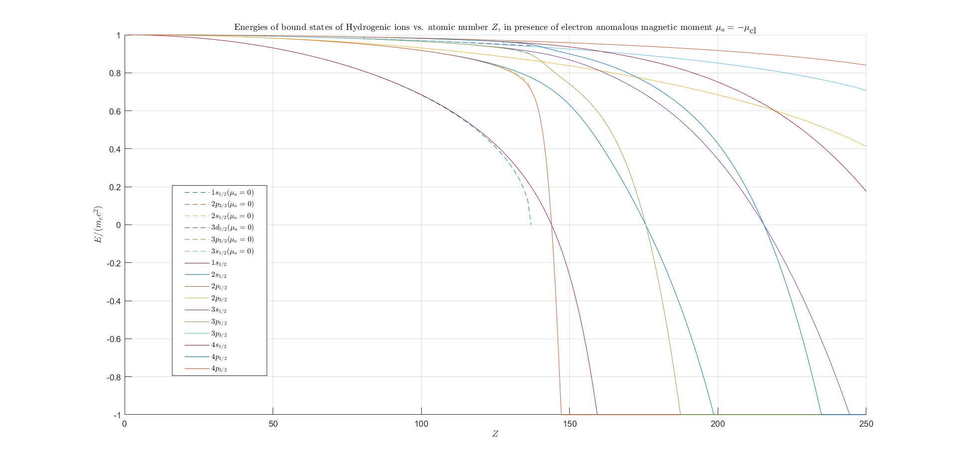
Figure 1: Electron Orbital Energies vs. the Nuclear Charge, with $\mathcal{G}<\mathcal{G}_{\mbox{\tiny res}}$

Our result here therefore conforms with (and confirms) Fig. 7.1 in [36].

A feature evident in Fig. 1 is that, even though our main result, Thm. 2.23, only holds for atomic numbers $Z\leq 45$, and only proves the existence of positive energy eigenvalues, the discrete spectrum apparently continues to exist beyond that range of $Z$ values, and far beyond nuclei found in nature or observed in the lab. It also appears to be the case, for any $n\geq 1$ and any nonzero $k\in\{-n,-n+1,\dots,n-1\}$, that as $Z$ is increased the energy continues to decrease, eventually crossing the $\varepsilon=0$ line and becoming negative, and finally touching the continuous spectrum at $\varepsilon=-1$. The restrictions in our theorem are therefore far from being optimal. Indeed, a rich list of phenomena seems to occur in this system beyond the range of $Z$ corresponding to nuclei so far observed in nature, phenomena that are awaiting to be studied by further careful mathematical analysis of the hamiltonian (2.25).

4 Summary and Outlook

4.1 Summary

In this paper we have supplied a complete characterization of the discrete Dirac spectrum of a point electron with fixed anomalous magnetic moment in the Reissner–Weyl–Nordström spacetime of a point nucleus, though only within certain ranges of the atomic number $Z$, the nuclear mass number $A$, and anomalous magnetic moment $\mu_{a}$. The $(Z,A)$ range contains approximately 50% of the empirically confirmed nuclei, from those of Hydrogen (H) to those of Rhodium (Rh), and allows us to form a one-to-one correspondence between the eigenfunctions of our hamiltonian and the orbitals of Hydrogen found in textbook quantum mechanics. The discrete spectrum is indexed by two integers $k$ and $N$, where $k$ is the eigenvalue of the spin-orbit operator, and $N$ can be identified with a topological winding number associated with a dynamical system on a compact cylinder that arises from the energy eigenvalue problem of our hamiltonian. The correspondence to the orbitals of Hydrogen is facilitated by defining a principal quantum number $n:=N+|k|$.

We also carried out a numerical study of the energy eigenvalues as a function of atomic number $Z$; however, we face a challenge: the gravitational coupling constant is so small that our algorithm cannot distinguish between the general and special relativistic problems.

Our numerical results conform with those in [36] that, as far as we can tell, nobody had tried to reproduce since their publication. Incidentally, note that the eigenvalues of $H$ appear to “dive into the negative continuum” when $Z$ becomes sufficiently large. However, by a result of Weidmann [40], the interior of the essential spectrum of the Dirac hamiltonian $H$ of an electron with anomalous magnetic moment is purely absolutely continuous, and this holds for whether the electron lives in the RWN spacetime of a point nucleus, or in the Minkowski spacetime equipped with a point nucleus. Hence, the statement ensuing Fig. 7.1 in [36], that the eigenvalues of the special-relativistic $H$ would dive into the lower continuum, should not be taken literally.

We emphasize the non-perturbative character of our paper, with its insistence on conceptual clarity that logically leads one to face the spectral questions we have addressed in this paper. In this regard it differs markedly from conventional inquiries into the effects of gravity on the hydrogenic spectra, e.g. [29], [28], which only consider the influence of an external gravitational field, and only in a perturbative manner. In a similar vein, our paper also differs markedly from conventional inquiries into the effect of the electron’s (and other leptons’) anomalous magnetic moment on the spectra, cf. [18], [14], [9].

4.2 Outlook

Having a well-defined general-relativistic Dirac operator for hydrogenic ions with nuclei that are treated as point particles, and having characterized its discrete spectrum (the essential spectrum had been identified earlier already, in [7]), the litmus test for the operator now is the question whether it has the correct energy spectrum, in the sense that its eigenvalue differences reproduce the empirical values of the Hydrogen frequencies within an empirically dictated margin of error. Since no empirical data exist for $Z>118$, the question is currently decidable only for when $Z\leq 118$. This question has not been addressed yet.

We emphasize that this question is more difficult to answer than the analogous question for the special-relativistic Dirac operator with the anomalous magnetic moment of the electron taken into account, which implicitly assumes that gravitational effects are negligible — precisely the assumption that one still has to vindicate rigorously. Yet, suppose for the sake of the argument right now that gravity is negligible. In that case the convergence in the regime $Z\leq 137$ of the spectrum of the special-relativistic Dirac operator with $\mu_{a}$ term to the spectrum of the distinguished self-adjoint extension of the one without it, when $\mu_{a}\to 0$, as noted in [21] and [33], is a very helpful piece of information to have. It allows one to work with the explicitly computable spectrum of the distinguished self-adjoint extension of the special-relativistic Dirac operator without $\mu_{a}$ term, plus $\mu_{a}$-dependent error bounds, to answer the question. By contrast, when not assuming that gravity is negligible, the analogous strategy does not work for general-relativistic problem with fixed $G>0$, because one can not take the limit $|\mu_{a}|\searrow 0$, only the limit $|\mu_{a}|\searrow\mu_{\rm crit}$, with $\mu_{\rm crit}$ given in (1.11), but this does not simplify the task at hand.

However, it is reasonable to conjecture that the spectrum of the general-relativistic Dirac hamiltonian in presence of the anomalous magnetic moment for the electron, converges to the corresponding special-relativistic Dirac spectrum as $\mathcal{G}$ (or equivalently, Newton’s constant of universal gravitation $G$) is sent to zero. For reasons described in section 3 and in the Introduction, this conjecture is easy to conceive but (we suspect) not so easy to prove. After all, our discussion in section 3 of the RWN metric function $f(r)$ is equally valid if the electron’s anomalous magnetic moment is absent from the Dirac hamiltonian, and in that case one knows through the work of Cohen and Powers [8] that the singular behavior of $f(r)$ as $r\to 0$ destroys the essential self-adjointness of the Dirac hamiltonian with $G=0$ for all $Z\leq 118$; the fact that $f(r)$ is practically 1 except for a tiny vicinity of $r=0$ is thus not a good guide for one’s intuition.

Be that as it may, we expect to be able to take the limit $G\searrow 0$ for $\mu_{a}$ fixed, which — if the point spectra converge to the special-relativistic $G=0$ spectra — would reduce the problem to understanding the special-relativistic Dirac spectrum with anomalous magnetic moment of the electron taken into account, which in turn can be estimated with the help of the strategy mentioned a few lines earlier. Yet, the $G\searrow 0$ limit has not been rigorously established yet. It is an interesting problem that we hope to return to in a future work.

Two interesting open questions concerning the Dirac hamiltonian of a point electron with fixed anomalous magnetic moment in either the RWN spacetime of a point nucleus, or the Minkowski spacetime equipped with a point nucleus, are suggested by Fig. 1. The first question is based on an observation already made in [36], namely the apparent level crossings at zero energy. Numerically we found that the crossings do not happen exactly at $E=0$, but the difference is so tiny that the deviation from $E=0$ may well be a numerical artifact. It would be good if it could be proved, or disproved, that level crossings happen precisely at $E=0$. The second question concerns the manner in which the eigenvalue curves meet the negative continuum. Do they meet it with a finite non-zero slope (treating $Z$ as real variable), or with a vanishing slope, or do they never meet the continuum but get asymptotically arbitrarily close to it? These are interesting mathematical questions.

Incidentally, supposing an eigenvalue curve actually meets the negative continuum at $Z=Z_{\circ}$, say, a natural question to ask in that case is whether $E=-m_{\mathrm{e}}c^{2}$ is then part of the point spectrum at $Z_{\circ}$. (It certainly could not be part of the discrete spectrum, as $E=-m_{\mathrm{e}}c^{2}$ belongs to the essential spectrum.) That question was already answered in [25], though, where a necessary condition was stated for $E=-m_{\mathrm{e}}c^{2}$ to be an eigenvalue of the Dirac operator of an electron with anomalous magnetic moment in electrostatic spacetimes of a point nucleus for a vast class of electromagnetic vacuum laws, see Thm. 3.25 in [25]. For the RWN spacetime this condition cannot be met in the naked singularity sector.

Another task for the future, motivated by physics, is to take the finite size of nuclei into account. At large $Z$ values, even in the range of the empirical nuclei, one risks stretching the validity of the point nucleus approximation beyond the estimable. Although the charge radius of a $Z=96$ nucleus is only a factor $\approx 7$ bigger than that of a proton (cf. the Nuclear Charge Radii website of the International Atomic Energy Commission), the electron in its ground state is then typically much closer to the nucleus than when $Z=1$, so that the charge distribution of the nucleus should begin to have a significant effect on the spectra.

A final thought on the problem of essential self-adjointness for hydrogenic ions, related to the finite size of the physical nuclei: It is often argued, cf. [36], that the problem of a lack of essential self-adjointness of the Dirac operator for hydrogenic ions (without anomalous magnetic moment of the electron) disappears if the nucleus is equipped with a continuously smeared out charge distribution rather than being treated as a point charge. However, this argument misses the point (pardon the pun) that nuclei are spatially extended bound states made of three point quarks, according to the standard model of elementary particle physics. Assuming that this standard model captures the nature of nuclei correctly, nuclei should fundamentally be associated with point charges when discussing hydrogenic (and other atomic / ionic) spectra, though the approximation to concentrate all the point charges at a single location is a simplification that turns into an over-simplification when $Z>118$ (as far as essential self-adjointness is concerned; for the spectra it presumably is an over-simplification already for smaller $Z$ values). Yet, since the charges of point quarks have magnitude not more than $\frac{2}{3}e$, it is conceivable that essential self-adjointness will hold for Dirac operators of an electron without anomalous magnetic moment in the Coulomb field of nuclei modeled as a sum of Dirac distributions of many point charges with magnitude not more than $\frac{2}{3}e$. We are not aware of any work that has addressed the hydrogenic Dirac problem for such models of nuclei. It should not be too difficult to address this problem in Minkowski spacetime. However, the general-relativistic problem will be formidable.

Another issue that needs to be addressed is whether $\mu_{a}$ changes significantly with the strength of the Coulomb field ($Z$), or the gravitational field ($M$). Our use of the classical value for the anomalous magnetic moment independently of $Z$ and of $M$, which is admissible for electrons in weak external fields, may be an oversimplification. In any event, by using a fixed $\mu_{a}(=-\mu_{cl})$ for all $Z$ and $M$ values we have followed the tradition [6], [15], [36], [7].

Appendix A The reduced Dirac hamiltonian as a linear matrix operator

As mentioned in section 2, the Dirac operator $H$ of a (test) electron with anomalous magnetic moment $\mu_{a}=-\mu_{\text{class}}$ in the RWN spacetime of a naked point nucleus of charge $Q=Ze$ and mass $M=A(Z,N)m_{\mathrm{p}}$ is essentially self-adjoint on the domain of $C^{\infty}$ bispinor wave functions which are compactly supported away from the singularity at $r=0$; see [7]. We also mentioned that this is so only because the physical value of the anomalous magnetic moment is larger (actually, much larger) than a critical value. This is in contrast to the corresponding problem on the Minkowski spacetime with point nucleus, where no critical anomalous magnetic moment has to be surpassed. In this appendix we briefly address the existence of a critical magnetic moment for the Dirac problem in the RWN spacetime versus its absence in the Minkowski spacetime.

Recall that due to the spherical symmetry and static character of the RWN and Minkowski spacetimes, the Dirac hamiltonian separates in the spherical coordinates and their default spin frame [8], resp. [36]. More precisely, $H$ is a direct sum of radial partial-wave Dirac operators $H^{\mbox{\tiny{rad}}}_{k}:=m_{\mathrm{e}}c^{2}K^{\mbox{\tiny{}}}_{k}$, $k\in\mathbb{Z}\backslash\{0\}$, cf. (2.17),

$$K_{k}^{\text{}}:=\left[\begin{array}[]{cc}f(r)-Z\alpha_{\mbox{\tiny{S}}}\frac{1}{r}&\left[\frac{k}{r}-Z\alpha_{\mbox{\tiny{S}}}^{2}\frac{1}{4\pi}\frac{1}{r^{2}}\right]f(r)-f^{2}(r)\tfrac{d}{dr}\\ \left[\frac{k}{r}-Z\alpha_{\mbox{\tiny{S}}}^{2}\frac{1}{4\pi}\frac{1}{r^{2}}\right]f(r)+f^{2}(r)\tfrac{d}{dr}&-f(r)-Z\alpha_{\mbox{\tiny{S}}}\frac{1}{r}\end{array}\right],$$ (A.46)

with $f(r)$ given in (2.23) for the RWN spacetime, while $f(r)\equiv 1$ for the Minkowski spacetime. Thus $H$ is essentially self-adjoint when all the operators $K^{\mbox{\tiny{}}}_{k}$ are, which act on $g(r):=\big{(}u(r),v(r)\big{)}^{T}\in C^{\infty}_{c}(\mathbb{R}_{+})^{2}$ equipped with a weighted $L^{2}$ norm given by

$$\|g\|^{2}:=\int_{0}^{\infty}\frac{1}{f^{2}(r)}\Big{(}|u(r)|^{2}+|v(r)|^{2}\Big{)}\mathrm{d}r;$$ (A.47)

cf. (2.18).

Setting $E_{k,d(k)}=:m_{\mathrm{e}}c^{2}\varepsilon_{k,d(k)}$, with $k\in\mathbb{Z}\backslash\{0\}$, and where $d(k)$ denotes a degeneracy label, the dimensionless eigenvalue problem reads

$$K^{\mbox{\tiny{}}}_{k}g(r)=\varepsilon_{k,d(k)}g(r).$$ (A.48)

With the essential spectrum equal to $(-\infty,-1]\cup[1,\infty)$ for either choice of $f$, see [7] and [36], we only need to address the regime $\varepsilon\in(-1,1)$. Even though the eigenvalue problem does not seem to be solvable in terms of known functions, special or not, whether $f(r)\equiv 1$ or given by (2.23), Weyl’s limit point / limit circle criterion [39] states that the issue of essential self-adjointness is decided by studying the asymptotic problems for when $r\nearrow\infty$ and when $r\searrow 0$.

For $r\nearrow\infty$ (A.48) becomes the free electron problem

$$\left[\begin{array}[]{cc}1&-\tfrac{d}{dr}\\ \tfrac{d}{dr}&-1\end{array}\right]\left[\begin{array}[]{c}u(r)\\ v(r)\end{array}\right]=\varepsilon\left[\begin{array}[]{c}u(r)\\ v(r)\end{array}\right];\qquad r\gg 1,$$ (A.55)

with $\varepsilon=\varepsilon_{k,d(k)}$, which has the well-known unique (up to an overall factor) $L^{2}([R,\infty))^{2}$ solution

$$\left[\begin{array}[]{c}u(r)\\ v(r)\end{array}\right]=\left[\begin{array}[]{c}C_{1}\\ C_{2}\end{array}\right]e^{-\sqrt{1-\varepsilon^{2}}\,r},$$ (A.60)

with $C_{1}$ and $C_{2}$ related by $C_{2}=-C_{1}/\sqrt{1-\varepsilon^{2}}$, and $C_{1}\equiv C$ to be determined subsequently. Note that this free electron asymptotics holds both for the RWN and for the Minkowski spacetime problems.

For the other asymptotic regime, as $r\searrow 0$, we need to distinguish the cases $f(r)\equiv 1$ and $f(r)$ given by (2.23). Beginning with the problem for the RWN spacetime, after factoring out $\mathcal{G}^{1/2}\alpha_{\mbox{\tiny{S}}}^{2}Z^{2}\frac{1}{r^{3}}$, equation (A.48) is asymptotic to the problem

$$\left[\begin{array}[]{cc}0&-\frac{\alpha_{\mbox{\tiny{S}}}}{4\pi}-{\mathcal{G}}^{1/2}r\tfrac{d}{dr}\\ -\frac{\alpha_{\mbox{\tiny{S}}}}{4\pi}+{\mathcal{G}}^{1/2}r\tfrac{d}{dr}&0\end{array}\right]\left[\begin{array}[]{c}u(r)\\ v(r)\end{array}\right]=\left[\begin{array}[]{c}0\\ 0\end{array}\right];\;r\ll 1.$$ (A.61)

Problem (A.61) has the one-dimensional $L^{2}((0,R])^{2}$ solution

$$\left[\begin{array}[]{c}u(r)\\ v(r)\end{array}\right]=\left[\begin{array}[]{c}B\\ 0\end{array}\right]r^{{\alpha_{\mbox{\tiny{S}}}}/{4\pi{\mathcal{G}}^{1/2}}},$$ (A.62)

with $B$ to be determined subsequently. Note that for the physical parameter values the power of the monomial is enormous, about $1.17\cdot 10^{18}$, so that the pertinent monomial with the negative of that power, viz. the second solution of (A.61), is not in $L^{2}((0,R],r^{2}dr)^{2}$. Therefore, for physical parameter values the operator $K_{k}$ is of limit point type at both ends, hence essentially self-adjoint on its minimal domain (cf. Theorem 2.6 and the remark after it). Note furthermore that the power is independent of $Z$, which in a nutshell is the reason for why the Dirac $H$ of an electron with (empirical-valued) anomalous magnetic moment in the RWN spacetime of a naked nucleus is essentially self-adjoint for all $Z$ values.

Yet, mathematically one can contemplate a world with different values of Newton’s constant of universal gravitation, everything else remaining untouched. Thus one can make $G$, hence $\mathcal{G}$ so large that also the monomial $r^{-{\alpha_{\mbox{\tiny{S}}}}/{4\pi{\mathcal{G}}^{1/2}}}\in L^{2}((0,R],r^{2}dr)$. In that case the operator is of limit circle type at $r=0$, while still of limit point type at $r=\infty$, and therefore not essentially self-adjoint. Alternatively to enlarging $G$ while keeping everything else fixed, one could also keep $G$ fixed and replace the anomalous magnetic moment of the electron by a fictiously small $\mu_{a}$ value (in magnitude), with the same conclusion of a not essentially self-adjoint $K_{k}$ when $|\mu_{a}|$ is small enough. The critical $|\mu_{a}|$ value is given in (1.11)

Note finally that the power is $\propto 1/\sqrt{\mathcal{G}}$, hence $\propto 1/\sqrt{G}$, which signals the highly non-trivial character of the problem of taking the mathematical zero-gravity limit $G\searrow 0$.

We now contrast $r\searrow 0$ asymptotics of the Dirac problem on RWN with its counterpart for the more familiar Dirac problem of a test electron with anomalous magnetic moment in the Coulomb field of a point nucleus in Minkowski space. The radial partial-wave Dirac operators $H^{\mbox{\tiny{rad}}}_{k}:=m_{\mathrm{e}}c^{2}K^{\mbox{\tiny{}}}_{k}$, $k\in\mathbb{Z}\backslash\{0\}$ now are given by

$$K_{k}^{\text{}}:=\left[\begin{array}[]{cc}1-Z\alpha_{\mbox{\tiny{S}}}\frac{1}{r}&k\frac{1}{r}-Z\frac{\alpha_{\mbox{\tiny{S}}}^{2}}{4\pi}\frac{1}{r^{2}}-\tfrac{d}{dr}\\ k\frac{1}{r}-Z\frac{\alpha_{\mbox{\tiny{S}}}^{2}}{4\pi}\frac{1}{r^{2}}+\tfrac{d}{dr}&-1-Z\alpha_{\mbox{\tiny{S}}}\frac{1}{r},\end{array}\right],$$ (A.63)

acting on $g(r):=\big{(}u(r),v(r)\big{)}^{T}\in C^{\infty}_{c}(\mathbb{R}_{+})^{2}$ equipped with an $L^{2}$ norm given by (A.47) with $f\equiv 1$. For the regime as $r\searrow 0$, after factoring out $\frac{1}{r^{2}}$, (A.48) now is asymptotic to the problem

$$\left[\begin{array}[]{cc}0&-Z\frac{\alpha_{\mbox{\tiny{S}}}^{2}}{4\pi}-{r^{2}}\tfrac{d}{dr}\\ -Z\frac{\alpha_{\mbox{\tiny{S}}}^{2}}{4\pi}+r^{2}\tfrac{d}{dr}&0\end{array}\right]\left[\begin{array}[]{c}u(r)\\ v(r)\end{array}\right]=\left[\begin{array}[]{c}0\\ 0\end{array}\right];\qquad r\ll 1,$$ (A.64)

which has the unique one-dimensional $L^{2}((0,R])^{2}$ solution

$$\left[\begin{array}[]{c}u(r)\\ v(r)\end{array}\right]=\left[\begin{array}[]{c}B\\ 0\end{array}\right]e^{-Z\frac{\alpha_{\mbox{\tiny{S}}}^{2}}{4\pi}\frac{1}{r}},$$ (A.65)

with $B$ to be determined subsequently. Notice that the second solution $\propto e^{Z\frac{\alpha_{\mbox{\tiny{S}}}^{2}}{4\pi}\frac{1}{r}}$ is not in $L^{2}((0,R],dr)^{2}$ for any $Z>0$, given $\alpha_{\mbox{\tiny{S}}}>0$. Hence the Dirac operator is of limit point type at both asymptotic ends, and therefore essentially self-adjoint on its minimal domain for all $Z>0$, and for all $\alpha_{\mbox{\tiny{S}}}^{2}>0$ — which means for any nontrivial anomalous magnetic moment of the electron $\mu_{a}\neq 0$.

Our discussion reveals a technical obstacle that needs to be overcome when trying to prove the conjecture that the essentially self-adjoint Dirac hamiltonian for an electron with physical anomalous magnetic moment on the RWN spacetime converges not only in strong resolvent sense but also in terms of its spectrum to the corresponding operator on the Minkowski spacetime when one takes the zero-gravity limit $G\searrow 0$. Manifestly the $L^{2}((0,R],r^{2}dr)$ function $r^{{\alpha_{\mbox{\tiny{S}}}}/{4\pi{\mathcal{G}}^{1/2}}}$ does not converge to the $L^{2}((0,R],dr)$ function $e^{-Z\frac{\alpha_{\mbox{\tiny{S}}}^{2}}{4\pi}\frac{1}{r}}$ when $G\searrow 0$. The $G\searrow 0$ limit presumably requires a study of the asymptotics beyond all orders, involving the theory of transseries [13]. Such a study has to be deferred to some future work.

References

- [1] G. Abramovici, Author correction: Incompatible Coulomb hamiltonian extensions, Sci. Rep. 10 (2020), 11170, 1–2.
- [2] , Incompatible Coulomb hamiltonian extensions, Sci. Rep. 10 (2020), 7280, 1–20.
- [3] V. Arnold, H. Kalf, and A. Schneider, Separated Dirac operators and asymptotically constant linear systems, Math. Proc. Cambridge Philos. Soc. 121 (1997), 141–146.
- [4] M. K. Balasubramanian, Scalar fields and spin-half fields on mildly singular spacetimes, Ph.D. thesis, Rutgers Univ. (2014), 1–77.
- [5] S. Basu, R. Pollack, and M.-F. Roy, Algorithms in real algebraic geometry, Springer, 2006.
- [6] H. Behncke, The Dirac equation with an anomalous magnetic moment, Math. Z. 174 (1980), 213–225.
- [7] F. Belgiorno, M. Martellini, and M. Baldicchi, Naked Reissner–Nordström singularities and the anomalous magnetic moment of the electron field, Phys. Rev. D 62 (2000), 084014.
- [8] J. M. Cohen and R. T. Powers, The general relativistic hydrogen atom, Commun. Math. Phys. 86 (1982), no. 1, 69 – 86.
- [9] A. Czarnecki, U. D. Jentschura, K. Pachucki, and V. A. Yerokhin, Anomalous magnetic moments of free and bound leptons, Can. J. Phys. 83 (2005), 1–9.
- [10] C. G. Darwin, The wave equation of the electron, Proc. Roy. Soc. London A118 (1928), 654–680.
- [11] S. Dasgupta, C. Khurana, and A. S. Tahvildar-Zadeh, One-dimensional hydrogenic ions with screened nuclear Coulomb field, arXiv:2312.04033 (2023), 1–25.
- [12] F. Dumortier, J. Llibre, and J. C. Artés, Qualitative theory of planar differential systems, Universitext, Springer-Verlag, Berlin, 2006.
- [13] J. Ecalle, Introduction aux fonctions analyzables et preuve constructive de la conjecture de Dulac, Actualités mathématiques, Hermann (Paris), 1992.
- [14] X. Fan, T. G. Myers, B. A. D. Sukra, and G. Gabrielse, Measurement of the electron magnetic moment, Phys. Rev. Lett. 130 (2023), 071801.
- [15] F. Gesztezy, B. Simon, and B. Thaller, On the self-adjointness of Dirac operators with anomalous magnetic moment, Proc. AMS 94 (1985), 115–118.
- [16] W. Gordon, Die Energieniveaus des Wasserstoffatoms nach der Diracschen Quantentheorie des Elektrons, Z. Phys. 48 (1928), 11–14.
- [17] W. Greiner, B. Müller, and J. Rafelski, Quantum electrodynamics of strong fields, Springer, 1985.
- [18] S. Guellati-Khelifa, Searching for new physics with the electron’s magnetic moment, Physics 16 (2023), 22.
- [19] The MathWorks Inc., Matlab version: 9.13.0 (r2022b), 2022.
- [20] U. D. Jentschura, Fine-structure constant for gravitational and scalar interactions, Phys. Rev. A 90 (2014), 022122.
- [21] H. Kalf and K. M. Schmidt, Spectral stability of the Coulomb–Dirac hamiltonian with anomalous magnetic moment, J. Diff. Eq. 205 (2004), 408–423.
- [22] T. Kato, Fundamental properties of hamiltonian operators of Schrödinger type, Trans. A.M.S. 70 (1951), 195–211.
- [23] M. K.-H. Kiessling, E. Ling, and A. S. Tahvildar-Zadeh, On the discrete Dirac spectrum of a point electron in the zero-gravity Kerr–Newman spacetime, J. Math. Phys. 63 (2022), no. 11, 112301.
- [24] M. K.-H. Kiessling and A. S. Tahvildar-Zadeh, The Dirac point electron in zero-gravity Kerr-Newman spacetime, J. Math. Phys. 56 (2015), 042303,1–43.
- [25] M. K.-H. Kiessling, A. S. Tahvildar-Zadeh, and E. Toprak, On general-relativistic hydrogen and hydrogenic ions, J. Math. Phys. 61 (2020), 092303,1–22.
- [26] H. Narnhofer, Quantum theory for potentials, Acta Phys. Austr. 40 (1974), 306–322.
- [27] G. Nordström, On the energy of the gravitational field in Einstein’s theory, Proc. Konigl. Ned. Akad. Wet. 20 (1918), 1238–1245.
- [28] L. Parker, One-electron atom as a probe of spacetime curvature, Phys. Rev. D 22 (1980), 1922–1934.
- [29] L. Parker and L. O. Pimentel, Gravitational perturbation of the hydrogen spectrum, Phys. Rev. D 25 (1982), 3180–3190.
- [30] L. Perko, Differential equations and dynamical systems, third ed., Texts in Applied Mathematics, vol. 7, Springer-Verlag, New York, 2001.
- [31] M. Reed and B. Simon, Methods of Modern Mathematical Physics, II, Acad. Press, 1975.
- [32] H. Reissner, Über die Eigengravitation des elektrischen Feldes nach der Einsteinschen Theorie, Annalen Phys. 59 (1916), 106–120.
- [33] K. M. Schmidt, Exceptional coupling constants for the Coulomb–Dirac operator with anomalous magnetic moment, J. Comput. Appl. Math. 194 (2006), 17–25.
- [34] E. Schrödinger, Quantisierung als Eigenwertproblem, Annalen Phys. 79 (1926), 361–376.
- [35] B. Thaller, Potential scattering of Dirac particles, J. Phys. A: Math. Gen. 14 (1981), 3067–3083.
- [36] , The Dirac equation, Springer-Verlag, Berlin, 1992.
- [37] , The Dirac operator. chpt. 2, pp. 23–106 in: Relativistic electronic structure theory. part 1. Fundamentals. Ed. Peter Schwerdtfeger, Theor. Comp. Chem. 11 (2002), 1–926.
- [38] J. H. Verner, Explicit Runge–Kutta pairs with lower stage-order, Numerical Algorithms 65 (2014), 555–577.
- [39] J. Weidmann, Oszillationsmethoden für Systeme gewöhnlicher Differentialgleichungen, Math. Z. 119 (1971), 349–373.
- [40] , Absolut stetiges Spektrum bei Sturm-Liouville-Operatoren und Dirac-Systemen, Math. Z. 180 (1982), no. 2, 423–427.
- [41] H. Weyl, Zur Gravitationstheorie, Annalen Phys. 54 (1917), 117–145.
- [42] I. Úlehla and J. Hořejši, Generalized Prüfer transformation and the eigenvalue problem for radial Dirac equations, Phys. Lett. A 113 (1986), no. 7, 355–358.