Abstract

Feature attributions are ubiquitous tools for understanding the predictions of machine learning models. However, popular methods for scoring input variables such as SHAP and LIME suffer from high instability due to random sampling. Leveraging ideas from multiple hypothesis testing, we devise attribution methods that correctly rank the most important features with high probability. Our algorithm RankSHAP guarantees that the $K$ highest Shapley values have the proper ordering with probability exceeding $1-\alpha$. Empirical results demonstrate its validity and impressive computational efficiency. We also build on previous work to yield similar results for LIME, ensuring the most important features are selected in the right order.

1 Introduction

Many machine learning (ML) algorithms have impressive predictive power but poor interpretability relative to simpler alternatives like decision trees and linear models. This tradeoff has motivated a wide body of work seeking to explain how black-box models make predictions [Belle and Papantonis, 2021]. Such work is essential for building trust in ML systems in areas like finance, healthcare, and criminal justice, in which the consequences of model misbehavior may be severe [Dubey and Chandani, 2022, Ferdous et al., 2020, Mandalapu et al., 2023, Berk, 2019]. Interpretable ML methods can also help develop understanding of complex processes, augmenting domain knowledge with new hypotheses.

To that end, feature attribution methods quantify the contributions of input features to the model’s performance. A wide range of methods have been proposed, detailed in Section 2, with subtle definitions and differences between them. In this paper, we argue that the particular value of an feature’s importance score is of less practical interest than their ranking: Which features are the most important, and the relative order of these highlighted features. A scientist using a machine learning model to predict disease risk from a patient’s genetic profile will priortize the genes with highest importance score for further study, with the ranking of the genes more relevant than the value of a particular importance metric. Similarly, explanations of individual predictions usually report only a small number of features in order not to overwhelm the user. LIME [Ribeiro et al., 2016], for example, explicitly regularizes to report a fixed number of features.

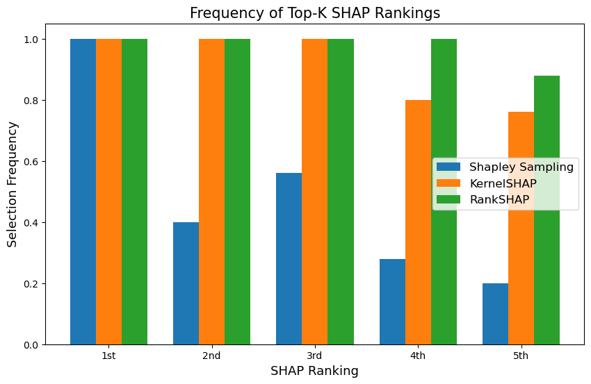
Figure 1: Instability of SHAP feature rankings, Wisconsin Breast Cancer dataset. Ordered attributions from Shapley Sampling and KernelSHAP with equal computational budget; RankSHAP has smaller budget. Details in Appendix A.1.

Unfortunately, many attribution methods including SHAP and LIME suffer from instability induced by random sampling. Thus, rerunning the same procedure could yield different explanations for which features are the most important. This inherent lack of reproducibility seriously undermines the credibility of these methods [Yu and Kumbier, 2020]. A number of adjustments have been shown to reduce the variability of the attribution values (e.g. KernelSHAP [Lundberg and Lee, 2017]); however, they do not necessarily stabilize the features’ rankings, which is much more salient. Figure 1 highlights the ranking instability of popular methods for computing SHAP values.

To address this, we propose sampling techniques for SHAP and LIME that identify the most important features in the correct order with high probability. Our method for Shapley values, RankSHAP, obtains the ranking of the $K$ highest-scoring features with probability exceeding $1-\alpha$. For LIME, we select the $K$ optimal features in the correct order along the LASSO path, with the same probabilistic guarantee.

Moreover, these methods are highly efficient. They spend the bulk of their computational work on features whose features whose rankings are both high and ambiguous, and run faster on inputs with clear feature orderings. Existing SHAP and LIME-based methods have no such adaptivity.

To our knowledge, this is the first work to control the error rate of sampling-based feature importance rankings and selections. Our method for LIME entails a simple modification of the S-LIME algorithm [Zhou et al., 2021]; therefore much of this paper is devoted to SHAP, and Shapley values more broadly.

2 Feature Importance Scores

2.1 Background

A broad range of research has addressed the question of how best to score input features to machine learning models. These explanations for model behavior can be on the level of individual predictions or aggregated across many samples (local or global). Many methods are specific to the particular choice of model, such as Breiman’s Mean Decrease in Impurity for random forests and the Feature Importance Ranking for neural networks [Breiman, 2001, Wojtas and Chen, 2020]. Breiman also proposed Permutation Importance, wherein the error of random forests is compared after permuting the values of each feature [Breiman, 2001]; this idea was later extended to the model-agnostic setting [Fisher et al., 2019]. Another model-agnostic technique, Leave-One-Covariate-Out (LOCO), compares the error after retraining the model without each feature [Lei et al., 2017].

SHAP and LIME are among the most popular feature importance methods. Both methods are model-agnostic and provide local explanations, although they can be easily adapted to the global setting [Covert et al., 2020]. We describe them in greater depth in the following subsections.

2.2 SHAP

In short, SHAP averages how much a feature influences the model’s prediction relative to subsets of the other features. It is a special case of the Shapley value, a seminal concept from game theory with numerous applications in machine learning [Shapley, 1952]. Lundberg and Lee show that Shapley values provide the only additive explanations that satisfy several reasonable desiderata [2017].

Shapley values score the $d$ “players” in a cooperative game, assessing their marginal contributions to all possible coalitions of teammates. (In the context of ML feature importances, $d$ is the number of the input features.) Let the value function $v:S\rightarrow\mathbb{R}$ evaluate the worth of coalition S. Further define $\Pi(d)$ as the set of all permutations of $[d]$, and $S_{j}^{\pi}\subseteq[d]\backslash\{j\}$ as the coalition of players that precede $j$ in permutation $\pi$. The Shapley value for player $j$ is defined as

$$\phi_{j}(v):=\frac{1}{d!}\sum_{\pi\in\Pi(d)}v(S_{j}^{\pi}\cup\{j\})-v(S_{j}^{\pi}).$$ (1)

Computing the Shapley value requires evaluating an exponential number of terms. When this is computationally prohibitive, it typically must be approximated via Monte Carlo sampling. Strumbelj and Kononenko proposed Shapley Sampling (Alg. 1), the most straightforward algorithm for doing so [2014]. This algorithm samples $n$ permutations at random, rather than using all $d!$. Trivially, it is an unbiased estimator of the true Shapley value.

Algorithm 1 Shapley Sampling

A Shapley value function $v(S)$, player $j\in[d]$, number of samples $n>0$

$\hat{\phi}_{j}(v)$, an unbiased estimate of $\phi_{j}(v)$

$\hat{\phi}_{j}\leftarrow 0$

for $i=1$ to $n$ do

     $\pi_{i}\leftarrow$ random permutation of $[d]$

     $S\leftarrow$ elements of $\pi_{i}$ before $j$

     $\hat{\phi}_{j}\leftarrow\hat{\phi}_{j}+v(S\cup\{j\})-v(S)$

end for

$\hat{\phi}_{j}(v)\leftarrow\frac{1}{n}\hat{\phi}_{j}(v)$

$$\hat{\phi}_{j}(v)=\frac{1}{n}\sum_{i=1}^{n}v(S_{j}^{i}\cup\{j\})-v(S_{j}^{i}).$$ (2)

How the value function $v(S)$ is defined does not affect the RankSHAP algorithm or its guarantees. Nevertheless, here we survey standard choices for Shapley-based feature importances. Some works advocate retraining the model on the coalition $S$ and taking its predictions [Strumbelj et al., 2009, Lipovetsky and Conklin, 2001]. Others take model predictions using observed data for the features in $S$ and random samples for the others. To select the random samples, methods including SHAP sample from their marginal distributions [Lundberg and Lee, 2017, Strumbelj and Kononenko, 2014] for practical ease. Alternative methods sample from approximations of the conditional distribution $X_{S^{c}}|X_{S}$ [Aas et al., 2021, Frye et al., 2020].

Several related works also seek to reduce the instability of Shapley estimates, including the popular KernelSHAP algorithm [Lundberg and Lee, 2017]. However, our method is the first to address rank instability. Moreover, our method can be applied in conjunction with several of these works [Mitchell et al., 2022, Illés and Kerényi, 2019, Goldwasser and Hooker, 2023].

2.3 LIME

LIME, or Local Interpretable Model-agnostic Explanations, is another standard technique in machine learning interpretability [Ribeiro et al., 2016]. The key idea is to create a simpler, inherently interpretable model in the vicinity of a specific prediction to help users understand the black-box model’s behavior at that point. It fits this explanation model on random samples generated around the input in question, labeled with the original model’s predictions.

The explanation model can be any predictor, e.g. a decision tree or ridge regression. LIME’s authors proposed using K-LASSO, a sparse linear model with $K$ nonzero coefficients. K-LASSO selects the $K$ features sequentially, generating the LASSO path with Least Angle Regression (LARS) [Tibshirani, 1996, Efron et al., 2004].

LIME with K-LASSO produces a form of feature attributions, in which only the $K$ features with nonzero coefficients are important. To compare the $K$ features’ importances, one may examine the order in which they enter the LASSO path. Alternatively, one can compare the regression coefficients, which may not be in the same order.

3 Rank Stability for Shapley Values

3.1 Problem Formulation

Let $(\hat{1}),(\hat{2}),\ldots,(\hat{d})$ be the order statistics of the Shapley estimates $\hat{\phi}_{j}\;\forall j$. That is, $(\hat{j})$ is the index of the feature with the j^th highest estimated Shapley value. We aim to estimate the true Shapley values $\phi_{j}$ such that the $K$ highest-ranking features are correctly ordered with probability at least $1-\alpha$. This goal can be formulated as the union of $K$ pairwise comparisons:

$$\{\phi_{(\hat{1})}\geq\phi_{(\hat{2})}\geq\ldots\geq\phi_{(\hat{K})}\geq\max_{j>K}\phi_{(\hat{j})}\}$$

$$\Longleftrightarrow\hskip 14.22636pt \Big{\{}\bigcup_{k=1}^{K}\phi_{(\hat{k})}\geq\max_{j>k}\phi_{(\hat{j})}\Big{\}}\hskip 28.45274pt\text{w.p. }\geq 1-\alpha.$$

Without loss of generality, one may choose to rank Shapley feature importances by their absolute values. We omit this in our mathematical formalization of the problem, but present it as an option in our code.

3.2 Pairwise Testing

We first consider testing $\phi_{(\hat{k})}\geq\max_{j>k}\phi_{(\hat{j})}$ in isolation, for any given $k\in[K]$. We want to develop a test that rejects the null hypothesis $H_{0}:\phi_{(\hat{k})}\leq\max_{j>k}\phi_{(\hat{j})}$ at significance level $\alpha$. For notational convenience, consider $k=1$, i.e. whether the feature with highest observed Shapley estimate is truly the most important.

Many works have developed tests to identify when the random variable with the largest observed value is indeed the object with the largest true value - here we use the “sample best” and “population best” to indicate these. Formally, let $X_{1},\ldots,X_{p}$ be drawn from distributions parametrized by unknown values $\theta_{1},\ldots,\theta_{p}\in\mathbb{R}$. Further let $(\hat{1}),\ldots,(\hat{p})$ estimate the ranking of the $\theta_{i}$ parameters based on the $X_{i}$ draws.

Hung and Fithian studied the setting where the random variables $X_{i}$ are drawn from distributions in the exponential family [2019]. They showed that any two-tailed test of $H_{0}:\theta_{(\hat{1})}=\theta_{(\hat{2})}$ is a valid level-$\alpha$ test for $H_{0}:\theta_{(\hat{1})}<\theta_{j>1}\phi_{(\hat{j})}$. That is, to determine the population best, it suffices to only compare the sample best to its runner up, so long as both tails are tested to account for selection. This is equivalent to performing a one-tailed test of $H_{0}:\theta_{(\hat{1})}\leq\theta_{(\hat{2})}$ at level $\frac{\alpha}{2}$.

The Shapley Sampling estimate of $\hat{\phi}_{j}$ (Eq. 2) is asymptotically a member of the exponential family. It is the average of $n_{j}$ independent and identically distributed (i.i.d.) draws of $v(S_{j}\cup\{j\})-v(S_{j})$. Therefore by the central limit theorem, it converges to a normal distribution with mean $\phi_{j}$ and variance $\sigma_{j}^{2}/n_{j}$, where $\sigma^{2}_{j}:=\text{Var}(v(S_{j}\cup\{j\})-v(S_{j}))$. Given a sufficiently large number of permutations, then, Hung and Fithian’s approach holds for testing whether the sample best is indeed the winner.

To find a valid pairwise test for Shapley estimates, we turn our focus to their asymptotic distribution. Assume without loss of generality that the first and second features are the sample best and runner up. Shapley Sampling samples permutations independently for different features, so $\hat{\phi}_{1}\perp\!\!\!\!\perp\hat{\phi}_{2}$. By the difference of Gaussian random variables,

$$\hat{\Delta}_{1}:=\hat{\phi}_{1}-\hat{\phi}_{2}\xRightarrow{d}\mathcal{N}\Big{(}\phi_{1}-\phi_{2},\frac{\sigma_{1}^{2}}{n_{1}}+\frac{\sigma_{2}^{2}}{n_{2}}\Big{)}.$$

The observed ordering is significant if reestimating $\phi_{1}$ and $\phi_{2}$ yields the same result with high probability. Formally, consider resampled Shapley estimates $\hat{\phi}_{1}^{*}$ and $\hat{\phi}_{2}^{*}$, with $\hat{\Delta}_{1}^{*}:=\hat{\phi}_{1}^{*}-\hat{\phi}_{2}^{*}$. Then the difference in differences has the asymptotic distribution

$$\hat{\Delta}_{1}^{*}-\hat{\Delta}_{1}\xRightarrow{d}\mathcal{N}\Big{(}0,2\Big{[}\frac{\sigma_{1}^{2}}{n_{1}}+\frac{\sigma_{2}^{2}}{n_{2}}\Big{]}\Big{)}.$$

While the true values of $\sigma_{j}^{2}$ are unknown, we can approximate them with the sample variances. This leads to the approximation

$$\hat{\Delta}_{1}^{*}|\hat{\Delta}_{1}\xRightarrow{d}\mathcal{N}\Big{(}\phi_{1}-\phi_{2},2\Big{[}\frac{\hat{\sigma}_{1}^{2}}{n_{1}}+\frac{\hat{\sigma}_{2}^{2}}{n_{2}}\Big{]}\Big{)}.$$

If $P(\hat{\Delta}_{1}^{*}<0|\hat{\Delta}_{1})<\frac{\alpha}{2}$, we can reject $H_{0}:\phi_{(\hat{1})}<\phi_{(\hat{2})}$ at level $\frac{\alpha}{2}$, thereby satisfying Hung and Fithian’s test for sample best. This occurs when

$$Z_{p_{n}}:=\frac{\hat{\Delta}_{1}}{\sqrt{2\Big{[}\frac{\hat{\sigma}_{1}^{2}}{n_{1}}+\frac{\hat{\sigma}_{2}^{2}}{n_{2}}\Big{]}}}\geq Z_{1-\alpha/2},$$ (3)

where $Z_{1-\alpha/2}$ is the $(1-\frac{\alpha}{2})$-level quantile of the standard normal distribution.

3.3 Multiple Testing

The previous subsection details conditions on which we can conclude $\phi_{(\hat{k})}\geq\max_{j>k}\phi_{(\hat{j})}$ at significance level $\alpha$. This problem of top-$K$ rank verification requires conducting $K$ such tests of sample best. This is a multiple testing problem, wherein we seek to control the family-wise error rate (FWER) at level $\alpha$. In this setting, the FWER is the probability that at least one estimated top-$K$ ranking is incorrect.

Normally, it is necessary to lower the significance level for each test in order to account for multiple testing. We discuss this in section 4, in the context of LIME. Here, however, no such adjustment is necessary. Hung and Fithian show that for exponential families, iteratively rejecting two-tailed level-$\alpha$ pairwise comparisons achieves FWER control for the rank verification problem [2019]. Thus, if all $K$ of the tests detailed in 3.2 reject, then the FWER is controlled at level $\alpha$.

3.4 RankSHAP Algorithm

Rearranging Eq. 3, the approximated Shapley values achieve FWER control when for all $k\in[K]$,

$$\hat{\Delta}_{k}:=\hat{\phi}_{(\hat{k})}-\hat{\phi}_{(\hat{k+1})}\geq Z_{1-\alpha/2}\sqrt{2\left[\frac{\hat{\sigma}_{(\hat{k})}^{2}}{n_{(\hat{k})}}+\frac{\hat{\sigma}_{(\hat{k+1})}^{2}}{n_{(\hat{k+1})}}\right]}.$$

If $\hat{\Delta}_{k}\sqrt{2\Big{[}\frac{\hat{\sigma}_{(\hat{k})}^{2}}{n_{(\hat{k})}}+\frac{\hat{\sigma}_{(\hat{k+1})}^{2}}{n_{(\hat{k+1})}}\Big{]}}^{-1}<Z_{1-\alpha/2}$ for some $k$, the $k$^th test fails to reject. In that case, it is necessary to run Shapley Sampling for more permutations on features $(\hat{k})$ and ${(\hat{k+1})}$, throwing out the data used thus far. Naively adding onto the original samples until the data is significant risks inflating the probability of a type I error. Alternatives to this approach which account for optional stopping are discussed in Section 6.

Simple calculations estimate the necessary number of samples to run. Suppose we want the new number of permutations to be the same $n^{\prime}$ for both features. Then setting $Z_{1-\alpha/2}\leq\hat{\Delta}_{k}\sqrt{2\Big{[}\frac{\hat{\sigma}_{(\hat{k})}^{2}}{n^{\prime}}+\frac{\hat{\sigma}_{(\hat{k+1})}^{2}}{n^{\prime}}\Big{]}}^{-1}$ leads to the sample size

$$n^{\prime}\geq 2\Big{(}\frac{Z_{1-\alpha/2}}{\hat{\Delta}_{k}}\Big{)}^{2}(\hat{\sigma}^{2}_{(\hat{k})}+\hat{\sigma}^{2}_{(\hat{k+1})}).$$ (4)

Alternatively, we may want the sample size to scale with the variance. Intuitively, more samples should be used for highly variable Shapley estimates. Defining $n_{(\hat{k+1})}^{\prime}:=\frac{\hat{\sigma}^{2}_{(\hat{k+1})}}{\hat{\sigma}^{2}_{(\hat{k})}}n_{(\hat{k})}^{\prime}$ and solving $Z_{1-\alpha/2}\leq\hat{\Delta}_{k}\sqrt{2\Big{[}\frac{\hat{\sigma}_{(\hat{k})}^{2}}{n_{(\hat{k})}^{\prime}}+\frac{\hat{\sigma}_{(\hat{k+1})}^{2}}{n_{(\hat{k+1})}^{\prime}}\Big{]}}^{-1}$ for $n_{(\hat{k})}^{\prime}$ yields

$$\begin{split}n_{(\hat{k})}^{\prime}&\geq 4\Big{(}\frac{Z_{1-\alpha/2}}{\hat{\Delta}_{k}}\Big{)}^{2}\hat{\sigma}^{2}_{(\hat{k})},\text{ and}\\ n_{(\hat{k+1})}^{\prime}&\geq 4\Big{(}\frac{Z_{1-\alpha/2}}{\hat{\Delta}_{k}}\Big{)}^{2}\hat{\sigma}^{2}_{(\hat{k+1})}.\end{split}$$ (5)

These lower bounds provide the minimum number of samples needed to obtain an anticipated significant result. To avoid narrowly missing the mark, it is reasonable to choose values of $n^{\prime}$ that exceed them by a small buffer, e.g. 10%.

Algorithm 2 RankSHAP

A Shapley value function $v(S)$, player set $[d]$, initial number of permutations $n_{0}$, number of features to rank correctly $K$, significance level $\alpha$, buffer $c$

Shapley value estimates whose top-$K$ rankings are correct with probability $\geq 1-\alpha$

for $i=1$ to $d$ do

     $\hat{\phi}_{j}\leftarrow$ Shapley Sampling estimate (Alg 1) with $n_{0}$ permutations on feature $j$

end for

while at least one test rejects do

     Find highest-ranked features whose significance test fails: lowest ${(\hat{k})}$, ${(\hat{k+1})}$ s.t.

$$(\hat{\phi}_{(\hat{k})}-\hat{\phi}_{(\hat{k+1})})\sqrt{2\Big{[}\frac{\hat{\sigma}_{(\hat{k})}^{2}}{n_{(\hat{k})}}+\frac{\hat{\sigma}_{(\hat{k+1})}^{2}}{n_{(\hat{k+1})}}\Big{]}}^{-1}<Z_{1-\alpha/2}.$$

     Solve for minimal $n_{(\hat{k})}^{\prime},n_{(\hat{k+1})}^{\prime}$ such that test rejects, with Eq. 4 or 5.

     $n_{(\hat{k})}^{\prime},n_{(\hat{k+1})}^{\prime}\leftarrow\lceil c*n_{(\hat{k})}^{\prime}\rceil,\lceil c*n_{(\hat{k+1})}^{\prime}\rceil$ 

     $\hat{\phi}_{(\hat{k})},\hat{\phi}_{(\hat{k+1})}\leftarrow$ Shapley Sampling with $n_{(\hat{k})}^{\prime},n_{(\hat{k+1})}^{\prime}$ permutations on ${(\hat{k})},{(\hat{k+1})}$.

end while

One important modification may be made to Algorithm 2. When consecutive Shapley values are very close to one another, RankSHAP may occasionally stipulate sampling unreasonably large numbers of permutations. In this case, it may be useful to only sample some maximal thresholding number.

Running for the maximal number of samples may actually suffice to produce statistically reproducible rankings, even when the anticipated number of required samples is higher. This is because the sample size calculations will be overinflated when the plug-in variance estimates underestimate the true variance (Eq. 4, 5), resulting in a heavy right tail in the distribution of $n^{\prime}$. Otherwise, the resulting Shapley estimates cannot be guaranteed to control the FWER. In that case, it may be necessary to lower $K$, raise $\alpha$, or increase the computational budget.

4 Rank Stability for LIME

LIME, introduced in section 2.3, fits an interpretable model on data randomly generated around a point of interest. Zhou et al. demonstrated how LIME’s inherent randomness induces substantial variability in the features selected by K-LASSO [2021]. To address this, they propose S-LIME, which applies hypothesis testing to each feature selection in LARS.

At each step, LARS iteratively chooses the predictor that is most correlated with the current residuals. S-LIME generates enough random samples until the feature’s sample correlation exceeds the runner-up’s with probability $1-\alpha$, where $\alpha$ is a user-specified significance level. We refer the reader to their manuscript for more detail.

Theorem 4.1.

Let the S-LIME algorithm be run with significance level $\frac{\alpha}{2K}$ for each pairwise test. Then the $K$ feature selections will choose the correct features in order with probability exceeding $1-\alpha$.

Proof. S-LIME compares scaled correlations $\hat{c}_{j}$, which are asmptotically normal by the central limit theorem. Because of this, rejecting a two-tailed level-$\alpha$ test between the first- and second-highest values of $c_{j}$ again suffices to show that the observed winner is indeed the most correlated of all available features. (In contrast, S-LIME performs a one-tailed level $\alpha$ test, so it can only conclude it is higher than the runner-up.) We can equivalently select the winner by performing a one-tailed test at level $\frac{\alpha}{2}$.

S-LIME performs $K$ such significance tests, so accounting for multiple testing is necessary. This requires adjusting the significance level, since we do not rank all $d$ statistics at once, as with Shapley values. The most straightforward way to achieve FWER control is with the Bonferroni Correction, which lowers each test’s threshold by a factor of the number of tests. Applying Bonferroni, setting the significance level for each test to $\frac{\alpha}{2K}$ implies that the probability of making at least one incorrect selection is at most $\alpha$. Therefore this procedure controls the FWER of the LARS selections along the LASSO path. ∎

5 Experiments

5.1 SHAP

Empirical results demonstrate RankSHAP’s ability to stabilize the rankings of feature attributions. First, we trained a neural network on the UCI Adult dataset to predict whether a person’s annual income exceeds $\$50,000$ [Kohavi, 1996]. This dataset contains 12 covariates of census information; computing each feature’s SHAP value exactly would require on the order of $2^{12}$ evaluations of the value function, motivating the use of sampling approximations.

We used a significance level of $\alpha=0.20$, indicating that the FWER should be at most $20\%$. On 30 input samples, we ran RankSHAP 250 times with both $K=2$ and $K=5$. To contextualize its performance, we also ran Shapley Sampling on the same 30 points, with a similar computational budget. For each input, we used 500 permutations per feature, as well as the average number of permutations used by RankSHAP.

To estimate the FWER for each sample, we counted the fraction of iterations that incorrectly ranked at least one of the top $K$ features. Figure 2 displays the observed FWERs for $K=2$ and $K=5$ on the Adult dataset. For all input samples and choices of $K$, RankSHAP successfully achieved FWER control. In contrast, FWERs of Shapley Sampling estimates exceeded 20% for a sizable proportion of inputs.

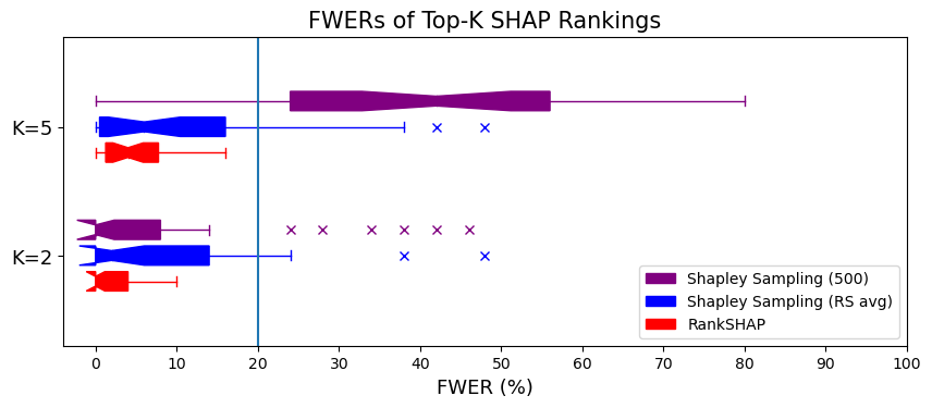
Figure 2: Boxplot of FWERs across 30 inputs, Adult Dataset. RankSHAP run with $\alpha=0.2$. For each input, Shapley Sampling uses 500 or RankSHAP’s average number of permutations across all 12 features.

We further evaluated RankSHAP’s performance across 5 benchmark datasets, training a neural network classifier on each (Table 1). On each dataset, we randomly selected 10 input samples from the test set, and ran RankSHAP 100 times with $K=3$ and $K=7$. Once again, RankSHAP typically achieved FWER control. The average empirical FWER on all datasets was below $\alpha=0.2$, reaching a maximum of 0.14 on the Wisconsin Breast Cancer dataset. The individual FWERs were always below $\alpha$ with $K=3$. For $K=7$, the few exceptions had empirical FWERs slightly above $0.2$; this was likely due to simulation variability, when based on 100 iterations.

			SHAP				LIME
	N	D	$\begin{subarray}{c}K=3,\\ \text{Avg FWER}\end{subarray}$	$\begin{subarray}{c}K=7,\\ \text{Avg FWER}\end{subarray}$	$\begin{subarray}{c}K=3,\\ \text{Prop }<\alpha\end{subarray}$	$\begin{subarray}{c}K=7,\\ \text{Prop }<\alpha\end{subarray}$	$\begin{subarray}{c}K=3,\\ \text{Avg FWER}\end{subarray}$	$\begin{subarray}{c}K=7,\\ \text{Avg FWER}\end{subarray}$	$\begin{subarray}{c}K=3,\\ \text{Prop }<\alpha\end{subarray}$	$\begin{subarray}{c}K=7,\\ \text{Prop }<\alpha\end{subarray}$
Adult	32,561	12	2%	14%	1	0.8	0%	NA	1	NA
Bank	45,211	16	6%	3%	1	1	0%	8%	1	0.9
BRCA	572	20	1%	7%	1	0.9	0%	12%	1	0.8
WBC	569	30	3%	10%	1	0.8	0%	NA	1	NA
Credit	1,000	20	1%	6%	1	1	0%	0%	1	1

Table 1: Stability of RankSHAP and LIME feature attributions. Both methods were run 100 times on 10 samples with $\alpha=0.2$, anticipating FWERs of at most 20%. Evaluated on Portuguese Bank, BRCA, Wisconsin Breast Cancer, Adult Census Income, and German Credit datasets, using neural network classifiers. NAs indicate the procedure does not reject all $K$ tests on the provided input samples.

Moreover, RankSHAP samples permutations in a highly efficient manner. While early ranking errors could lead RankSHAP to consider more than the top-ranked features, Figure 3 demonstrates that this happens rarely, with most features only needing the initial 100 permutations. Instead, it adaptively focuses its computational efforts on the features whose rankings are both ambiguous and relatively high. In this case, to rank the top $K$ features, extra samples are only regularly needed for the top $K+1$. In contrast, existing Shapley estimation algorithms allot the same budget for all features. This explains why Shapley Sampling with the same total number of samples often failed to control the FWER (Fig. 2).

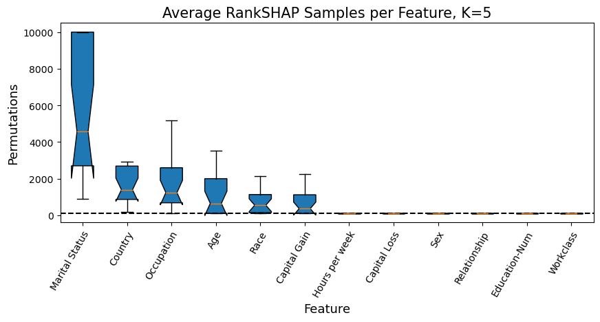
Figure 3: Number of permutations for each feature. On Adult dataset, $K=5$. Dashed line at initialization of 100 samples. Outliers omitted.

5.2 LIME

Experiments show our procedure for LIME controls the FWER of its sequential feature selections. We trained a random forest to classify malignant versus benign tumors on the UCI Breast Cancer dataset [Breiman, 2001, Wolberg et al., 1995]. The 30 covariates characterize the cell nuclei on tumor regions - for example, their area, perimeter, or smoothness.

Table 2: Frequencies of observed FWERs of LIME method with $\alpha=0.20$, across 30 samples.

K (# features)	0	0.01-0.05	0.06-0.2	$>0.2$
2	22	8	0	0
5	18	12	0	0

Again, we used a significance level of $\alpha=0.2$ for $K=2$ and $5$. We ran our method across 30 data samples from the test set, estimating FWER across 250 iterations. As anticipated, the empirical FWER is always below 20%. In fact, the FWER for over half of samples was 0 for both values of $K$ (Table 2). Figure 4 compares our method to the standard LIME algorithm with default parameters. It shows dramatically improved stability in the order of LIME feature selections.

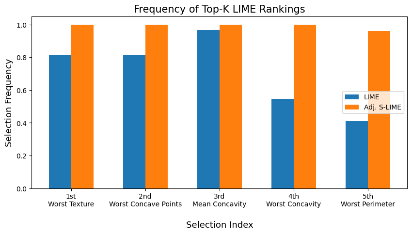
Figure 4: Stability of LIME selections on features 1 through $K$, around same sample. LIME uses default of 5,000 samples.

Evaluating our LIME method on the same 5 datasets demonstrated consistent FWER control. Table 1 highlights that it controls FWER on most inputs, and all datasets in the average case. For $K=7$, however, two datasets did not have inputs whose rank stability could be assured with the given sample budget. This is in part because the threshold for each test, $\frac{\alpha}{2K}$, becomes more restrictive as the number of desired rankings grows.

That these FWERs tend to be far below the significance level indicates that our approach may be fairly conservative. If this is indeed the case, it may be accounted for by the fact that the Bonferroni Correction is known to be conservative when tests are positively correlated [Bender and Lange, 1999]. Future work could apply more powerful testing procedures in this context. However, due to its sequential nature, standard FWER-controlling alternatives like Holm’s method cannot apply [Holm, 1979].

More detailed information concerning these experiments are in the Appendix.

6 Discussion

In this paper we present methods to obtain stable orderings of feature importance scores. Our algorithms guarantee that the probability of an incorrect Shapley ranking or LIME selection of a top-$K$ feature is at most $\alpha$.

As mentioned previously, RankSHAP can be used to rank Shapley values in any context, not specifically for SHAP. For example, it can be used for Shapley feature importances that sample from conditional distributions [Aas et al., 2021, Frye et al., 2020]. Shapley values also are used in machine learning for feature selection [Cohen et al., 2007], federated learning [Liu et al., 2022], data valuation [Ghorbani and Zou, 2019], multi-agent RL [Li et al., 2021], and ensembling [Rozemberczki and Sarkar, 2021].

Further, Shapley values have numerous applications outside of ML. They were originally studied in game theory, allocating credit to players in a cooperative game. Works have applied them in fields as diverse as ecology [Haake et al., 2007], online advertising [Zhao et al., 2018], supply chain management [Xu et al., 2018], and financial portfolio optimization [Shalit, 2020].

In addition to its analytical utility, RankSHAP runs relatively quickly. It avoids precise estimation of Shapley values for features whose rankings are low or unambiguous. In its current form, RankSHAP samples permutations from scratch when a test fails to reject. Future work may keep these permutations, and adjust the significance level to account for optional stopping. Potentially relevant methods include sequential probability ratio testing [Wald, 1945, Rushton, 1952, Hajnal, 1961], group-sequential testing [Pocock, 1977, O’Brien and Fleming, 1979], safe testing [Grünwald et al., 2019], and always valid p-values [Johari et al., 2019].

Various works have attempted to stabilize SHAP and LIME explanations [Goldwasser and Hooker, 2023, Mitchell et al., 2022, Zhou et al., 2021]. While these methods are useful, they may be less relevant, as reducing the variance does not necessarily translate into stabilizing rankings. In contrast, RankSHAP provides concrete statistical guarantees on feature rankings and selections, strengthening these tools’ capacity for meaningful analysis.

Impact Statement

This work has positive ethical and societal consequences, as it enables more trustworthy examination of machine learning models. Ultimately, we hope this improves the accountability of models used in high-stakes domains like criminal justice and healthcare.

However, feature attribution methods are imperfect for reasons well beyond their sampling variability. For example, different explanation methods may not agree on which methods are most important; in addition, their attributions may be highly sensitive to the idiosyncracies of the particular model. Thus, while our methods should instill greater trust in SHAP and LIME explanations, they alone are not enough to gauge whether models should be used in potentially harmful contexts. Rather, they are helpful tools that should be used in conjunction with a broader critical analysis.

Appendix A Experimental Details

For all experiments, we ranked the absolute values of SHAP values. The sum of all SHAP values for input $x$ is $f(x)-E[f(X)]$, which may be positive or negative. In the latter case, the most important features are the ones with the largest negative values. Further, an individual sample may have features with both large positive and negative SHAP values.

A.1 Figure 1

We ran the Shapley Sampling and KernelSHAP implementations in the shap package. Each used a total of $500\times d=6000$ permutations. RankSHAP, run with $K=5$ and $\alpha=0.2$, used a maximum of 500 permutations per feature. We kept the runs that failed to converge. The top-5 FWERs were 0.92, 0.24, and 0.12, respectively.

A.2 RankSHAP

The census dataset (Adult) has 48,842 samples before data preprocessing and splitting. Its labels have a roughly 3:1 imbalance, where 75% of the samples are individuals earning less than $\$50k$.

We trained a two-layer feedforward neural network in Pytorch for 20 epochs. The hidden layer had 50 neurons. To discourage overfitting to the more common class, we batched the two classes in sampling each batch from the training data. The test-set accuracy of the trained network was 82%.

To estimate the Shapley values, each run used 100 initial permutations per feature, and a maximum of 10000. For sample size calculations, we scaled $n^{\prime}_{(\hat{k})}$ and $n^{\prime}_{(\hat{k+1})}$ according to their relative variances (Eq. 5, not 4).

We only considered input samples for which RankSHAP successfully rejected all tests on at least 50% of the iterations (3.2). We applied the same selection criterion to LIME, detailed below.

A.3 LIME

The Wisconsin Breast Cancer dataset was much smaller, with only 569 total samples. 63% of the tissues are benign, and the remaining 37% are malignant. We trained sklearn’s RandomForestClassifier() with default settings. This attains over 94% classification accuracy.

Our procedure can be implemented using Zhengze Zhou’s slime repository almost entirely off-the-shelf. In our experiments, we added only 3 lines of code, which flag when the maximum number of samples have been used but not all hypothesis tests reject.

To control FWER at level $\alpha$, the “alpha” parameter passed to slime() should be $\frac{\alpha}{2K}$. We used 1,000 initial samples, and a maximum of 200,000. Another parameter, “tol,” denotes the tolerance level of the hypothesis tests. Setting $tol=0$ corresponds to the algorithm in the paper, and is of course a viable option. The creators of the package found that having a small positive tolerance could yield the same results with considerably greater efficiency. We set $tol=1*10^{-4}$, which ran more quickly while controlling the FWER at level $\alpha$.

References

- Aas et al. [2021] K. Aas, M. Jullum, and A. Løland. Explaining individual predictions when features are dependent: More accurate approximations to shapley values. Artif. Intell., 298:103502, 2021. doi: 10.1016/J.ARTINT.2021.103502. URL https://doi.org/10.1016/j.artint.2021.103502.
- Belle and Papantonis [2021] V. Belle and I. Papantonis. Principles and practice of explainable machine learning. Frontiers Big Data, 4:688969, 2021. doi: 10.3389/fdata.2021.688969. URL https://doi.org/10.3389/fdata.2021.688969.
- Bender and Lange [1999] R. Bender and S. Lange. Multiple test procedures other than bonferroni’s deserve wider use. BMJ, 318(7183):600–601, Feb 27 1999. doi: 10.1136/bmj.318.7183.600a.
- Berk [2019] R. Berk. Machine Learning Risk Assessments in Criminal Justice Settings. Springer, 2019. ISBN 978-3-030-02271-6. doi: 10.1007/978-3-030-02272-3. URL https://doi.org/10.1007/978-3-030-02272-3.
- Breiman [2001] L. Breiman. Random forests. Mach. Learn., 45(1):5–32, 2001. doi: 10.1023/A:1010933404324. URL https://doi.org/10.1023/A:1010933404324.
- Cohen et al. [2007] S. B. Cohen, G. Dror, and E. Ruppin. Feature selection via coalitional game theory. Neural Comput., 19(7):1939–1961, 2007. doi: 10.1162/NECO.2007.19.7.1939. URL https://doi.org/10.1162/neco.2007.19.7.1939.
- Covert et al. [2020] I. Covert, S. M. Lundberg, and S. Lee. Understanding global feature contributions through additive importance measures. CoRR, abs/2004.00668, 2020. URL https://arxiv.org/abs/2004.00668.
- Dubey and Chandani [2022] R. Dubey and A. Chandani. Application of machine learning in banking and finance: a bibliometric analysis. Int. J. Data Anal. Tech. Strateg., 14(3), 2022. doi: 10.1504/ijdats.2022.128268. URL https://doi.org/10.1504/ijdats.2022.128268.
- Efron et al. [2004] B. Efron, T. Hastie, I. Johnstone, and R. Tibshirani. Least angle regression. The Annals of Statistics, 32(2):407–451, 2004. ISSN 00905364. URL http://www.jstor.org/stable/3448465.
- Ferdous et al. [2020] M. Ferdous, J. Debnath, and N. R. Chakraborty. Machine learning algorithms in healthcare: A literature survey. In 11th International Conference on Computing, Communication and Networking Technologies, ICCCNT 2020, Kharagpur, India, July 1-3, 2020, pages 1–6. IEEE, 2020. doi: 10.1109/ICCCNT49239.2020.9225642. URL https://doi.org/10.1109/ICCCNT49239.2020.9225642.
- Fisher et al. [2019] A. Fisher, C. Rudin, and F. Dominici. All models are wrong, but many are useful: Learning a variable’s importance by studying an entire class of prediction models simultaneously. J. Mach. Learn. Res., 20:177:1–177:81, 2019. URL http://jmlr.org/papers/v20/18-760.html.
- Frye et al. [2020] C. Frye, C. Rowat, and I. Feige. Asymmetric shapley values: incorporating causal knowledge into model-agnostic explainability. In H. Larochelle, M. Ranzato, R. Hadsell, M. Balcan, and H. Lin, editors, Advances in Neural Information Processing Systems 33: Annual Conference on Neural Information Processing Systems 2020, NeurIPS 2020, December 6-12, 2020, virtual, 2020. URL https://proceedings.neurips.cc/paper/2020/hash/0d770c496aa3da6d2c3f2bd19e7b9d6b-Abstract.html.
- Ghorbani and Zou [2019] A. Ghorbani and J. Zou. Data shapley: Equitable valuation of data for machine learning, 2019.
- Goldwasser and Hooker [2023] J. Goldwasser and G. Hooker. Stabilizing estimates of shapley values with control variates. CoRR, abs/2310.07672, 2023. doi: 10.48550/ARXIV.2310.07672. URL https://doi.org/10.48550/arXiv.2310.07672.
- Grünwald et al. [2019] P. Grünwald, R. de Heide, and W. M. Koolen. Safe testing. CoRR, abs/1906.07801, 2019. URL http://arxiv.org/abs/1906.07801.
- Haake et al. [2007] C.-J. Haake, A. Kashiwada, and F. E. Su. The shapley value of phylogenetic trees. Journal of Mathematical Biology, 56(4):479–497, Sept. 2007. ISSN 1432-1416. doi: 10.1007/s00285-007-0126-2. URL http://dx.doi.org/10.1007/s00285-007-0126-2.
- Hajnal [1961] J. Hajnal. A two-sample sequential t-test. Biometrika, 48(1-2):65–75, 06 1961. ISSN 0006-3444. doi: 10.1093/biomet/48.1-2.65. URL https://doi.org/10.1093/biomet/48.1-2.65.
- Holm [1979] S. Holm. A simple sequentially rejective multiple test procedure. Scandinavian Journal of Statistics, 6(2):65–70, 1979.
- Hung and Fithian [2019] K. Hung and W. Fithian. Rank verification for exponential families. The Annals of Statistics, 47(2), Apr. 2019. ISSN 0090-5364. doi: 10.1214/17-aos1634. URL http://dx.doi.org/10.1214/17-AOS1634.
- Illés and Kerényi [2019] F. Illés and P. Kerényi. Estimation of the shapley value by ergodic sampling. CoRR, abs/1906.05224, 2019. URL http://arxiv.org/abs/1906.05224.
- Johari et al. [2019] R. Johari, L. Pekelis, and D. J. Walsh. Always valid inference: Bringing sequential analysis to a/b testing, 2019.
- Kohavi [1996] R. Kohavi. Census income. https://doi.org/10.24432/C5GP7S, Apr. 1996. URL https://doi.org/10.24432/C5GP7S.
- Lei et al. [2017] J. Lei, M. G’Sell, A. Rinaldo, R. J. Tibshirani, and L. Wasserman. Distribution-free predictive inference for regression, 2017.
- Li et al. [2021] J. Li, K. Kuang, B. Wang, F. Liu, L. Chen, F. Wu, and J. Xiao. Shapley counterfactual credits for multi-agent reinforcement learning. In F. Zhu, B. C. Ooi, and C. Miao, editors, KDD ’21: The 27th ACM SIGKDD Conference on Knowledge Discovery and Data Mining, Virtual Event, Singapore, August 14-18, 2021, pages 934–942. ACM, 2021. doi: 10.1145/3447548.3467420. URL https://doi.org/10.1145/3447548.3467420.
- Lipovetsky and Conklin [2001] S. Lipovetsky and M. Conklin. Analysis of regression in game theory approach. Applied Stochastic Models in Business and Industry, 17(4):319–330, October 2001. doi: 10.1002/asmb.446. URL https://ideas.repec.org/a/wly/apsmbi/v17y2001i4p319-330.html.
- Liu et al. [2022] Z. Liu, Y. Chen, H. Yu, Y. Liu, and L. Cui. Gtg-shapley: Efficient and accurate participant contribution evaluation in federated learning. ACM Trans. Intell. Syst. Technol., 13(4):60:1–60:21, 2022. doi: 10.1145/3501811. URL https://doi.org/10.1145/3501811.
- Lundberg and Lee [2017] S. M. Lundberg and S. Lee. A unified approach to interpreting model predictions. In I. Guyon, U. von Luxburg, S. Bengio, H. M. Wallach, R. Fergus, S. V. N. Vishwanathan, and R. Garnett, editors, Advances in Neural Information Processing Systems 30: Annual Conference on Neural Information Processing Systems 2017, December 4-9, 2017, Long Beach, CA, USA, pages 4765–4774, 2017. URL https://proceedings.neurips.cc/paper/2017/hash/8a20a8621978632d76c43dfd28b67767-Abstract.html.
- Mandalapu et al. [2023] V. Mandalapu, L. Elluri, P. Vyas, and N. Roy. Crime prediction using machine learning and deep learning: A systematic review and future directions. IEEE Access, 11:60153–60170, 2023. doi: 10.1109/ACCESS.2023.3286344. URL https://doi.org/10.1109/ACCESS.2023.3286344.
- Mitchell et al. [2022] R. Mitchell, J. Cooper, E. Frank, and G. Holmes. Sampling permutations for shapley value estimation. J. Mach. Learn. Res., 23:43:1–43:46, 2022. URL http://jmlr.org/papers/v23/21-0439.html.
- O’Brien and Fleming [1979] P. C. O’Brien and T. R. Fleming. A multiple testing procedure for clinical trials. Biometrics, 35(3):549–556, 1979. ISSN 0006341X, 15410420. URL http://www.jstor.org/stable/2530245.
- Pocock [1977] S. J. Pocock. Group sequential methods in the design and analysis of clinical trials. Biometrika, 64(2):191–199, 1977. ISSN 00063444. URL http://www.jstor.org/stable/2335684.
- Ribeiro et al. [2016] M. T. Ribeiro, S. Singh, and C. Guestrin. ”why should I trust you?”: Explaining the predictions of any classifier. In B. Krishnapuram, M. Shah, A. J. Smola, C. C. Aggarwal, D. Shen, and R. Rastogi, editors, Proceedings of the 22nd ACM SIGKDD International Conference on Knowledge Discovery and Data Mining, San Francisco, CA, USA, August 13-17, 2016, pages 1135–1144. ACM, 2016. doi: 10.1145/2939672.2939778. URL https://doi.org/10.1145/2939672.2939778.
- Rozemberczki and Sarkar [2021] B. Rozemberczki and R. Sarkar. The shapley value of classifiers in ensemble games. In G. Demartini, G. Zuccon, J. S. Culpepper, Z. Huang, and H. Tong, editors, CIKM ’21: The 30th ACM International Conference on Information and Knowledge Management, Virtual Event, Queensland, Australia, November 1 - 5, 2021, pages 1558–1567. ACM, 2021. doi: 10.1145/3459637.3482302. URL https://doi.org/10.1145/3459637.3482302.
- Rushton [1952] S. Rushton. On a two-sided sequential t-test. Biometrika, 39:302–308, 1952. URL https://api.semanticscholar.org/CorpusID:119952304.
- Shalit [2020] H. Shalit. The shapley value of regression portfolios. Journal of Asset Management, 21(6):506–512, 2020. URL https://EconPapers.repec.org/RePEc:pal:assmgt:v:21:y:2020:i:6:d:10.1057_s41260-020-00175-0.
- Shapley [1952] L. Shapley. A value for n-person games, march 1952.
- Strumbelj and Kononenko [2014] E. Strumbelj and I. Kononenko. Explaining prediction models and individual predictions with feature contributions. Knowl. Inf. Syst., 41(3):647–665, 2014. doi: 10.1007/S10115-013-0679-X. URL https://doi.org/10.1007/s10115-013-0679-x.
- Strumbelj et al. [2009] E. Strumbelj, I. Kononenko, and M. Robnik-Sikonja. Explaining instance classifications with interactions of subsets of feature values. Data Knowl. Eng., 68(10):886–904, 2009. doi: 10.1016/J.DATAK.2009.01.004. URL https://doi.org/10.1016/j.datak.2009.01.004.
- Tibshirani [1996] R. Tibshirani. Regression shrinkage and selection via the lasso. Journal of the Royal Statistical Society. Series B (Methodological), 58(1):267–288, 1996. ISSN 00359246.
- Wald [1945] A. Wald. Sequential tests of statistical hypotheses. Annals of Mathematical Statistics, 16:117–186, 1945.
- Wojtas and Chen [2020] M. Wojtas and K. Chen. Feature importance ranking for deep learning. In H. Larochelle, M. Ranzato, R. Hadsell, M. Balcan, and H. Lin, editors, Advances in Neural Information Processing Systems 33: Annual Conference on Neural Information Processing Systems 2020, NeurIPS 2020, December 6-12, 2020, virtual, 2020. URL https://proceedings.neurips.cc/paper/2020/hash/36ac8e558ac7690b6f44e2cb5ef93322-Abstract.html.
- Wolberg et al. [1995] W. Wolberg, O. Mangasarian, N. Street, and W. Street. Breast Cancer Wisconsin (Diagnostic). UCI Machine Learning Repository, 1995. DOI: https://doi.org/10.24432/C5DW2B.
- Xu et al. [2018] Z. Xu, Z. Peng, L. Yang, and X. Chen. An improved shapley value method for a green supply chain income distribution mechanism. International Journal of Environmental Research and Public Health, 15(9):1976, Sep 2018. doi: 10.3390/ijerph15091976.
- Yu and Kumbier [2020] B. Yu and K. Kumbier. Veridical data science. Proceedings of the National Academy of Sciences, 117(8):3920–3929, Feb. 2020. ISSN 1091-6490. doi: 10.1073/pnas.1901326117. URL http://dx.doi.org/10.1073/pnas.1901326117.
- Zhao et al. [2018] K. Zhao, S. H. Mahboobi, and S. R. Bagheri. Shapley value methods for attribution modeling in online advertising, 2018.
- Zhou et al. [2021] Z. Zhou, G. Hooker, and F. Wang. S-lime: Stabilized-lime for model explanation. In Proceedings of the 27th ACM SIGKDD Conference on Knowledge Discovery and Data Mining, KDD ’21. ACM, Aug. 2021. doi: 10.1145/3447548.3467274. URL http://dx.doi.org/10.1145/3447548.3467274.