The Discrepancy of Shortest Paths

Abstract

The hereditary discrepancy of a set system is a certain quantitative measure of the pseudorandom properties of the system. Roughly, hereditary discrepancy measures how well one can $2$-color the elements of the system so that each set contains approximately the same number of elements of each color. Hereditary discrepancy has well-studied applications e.g. in communication complexity and derandomization. More recently, the hereditary discrepancy of set systems of shortest paths has found applications in differential privacy [Chen et al. SODA 23].

The contribution of this paper is to improve the upper and lower bounds on the hereditary discrepancy of set systems of unique shortest paths in graphs. In particular, we show that any system of unique shortest paths in an undirected weighted graph has hereditary discrepancy $\widetilde{O}(n^{1/4})$, and we construct lower bound examples demonstrating that this bound is tight up to hidden $\text{polylog }n$ factors. Our lower bounds apply even in the planar and bipartite settings, and they improve on a previous lower bound of $\Omega(n^{1/6})$ obtained by applying the trace bound of Chazelle and Lvov [SoCG’00] to a classical point-line system of Erdős. We also show similar bounds on (non-hereditary) discrepancy and in the setting of directed graphs.

As applications, we improve the lower bound on the additive error for differentially-private all pairs shortest distances from $\Omega(n^{1/6})$ [Chen et al. SODA 23] to $\Omega(n^{1/4})$, and we improve the lower bound on additive error for the differentially-private all sets range queries problem to $\Omega(n^{1/4})$, which is tight up to hidden $\text{polylog }n$ factors [Deng et al. WADS 23].

1 Introduction

In graph algorithms, a fundamental problem is to efficiently compute distance or shortest path information of a given input graph. Over the last decade or so, the community has increasingly sought a principled understanding of the combinatorial structure of shortest paths, with the goal to exploit this structure in algorithm design. That is, in various graph settings, we can ask:

What notable structural properties hold for shortest path systems, that do not necessarily hold for arbitrary path systems?

The following are a few of the major successes of this line of work:

• An extremely popular strategy in the literature is to use hitting sets, in which we (often randomly) generate a set of nodes $S$ and argue that it will hit a shortest path for every pair of nodes that are sufficiently far apart. Hitting sets rarely exploit any structure of shortest paths, as evidenced by the fact that most hitting set algorithms generalize immediately to arbitrary set systems. However, they have inspired a successful line of work into graphs of bounded highway dimension [AFGW10, BDG⁺16, BDF⁺22]; very roughly, these are graphs whose shortest paths admit unusually efficient hitting sets of a certain kind.

• Shortest paths exhibit the notable structural property of consistency, i.e., any subpath of a shortest path is itself a shortest path. This fact is used throughout the literature on graph algorithms [CE06, CLRS22, Bod19], including e.g. in the classic Floyd-Warshall algorithm for All-Pairs Shortest Paths. A recent line of work has sought to characterize the additional structure exhibited by shortest path systems, beyond consistency [Bod19, CE06, CL22, CL23, CCL23b, AW20, AW23].

• Planar graphs have received special attention within this research program, and planar shortest path systems carry some notable additional structure. For example, it is known that planar shortest paths have unusually efficient tree coverings [Bal22, CCL⁺23a], and that their shortest paths can be compressed into surprisingly small space [CGMW18, CKT22]. Shortest path algorithms also often benefit from more general structural facts about planar graphs, such as separator theorems [HKRS97, HP11].

The main result of this paper is a new structural separation between shortest path systems and arbitrary path systems, expressed through the lens of discrepancy theory. We will come to formal definitions of discrepancy in just a moment, but at a high level, discrepancy has been described as a quantitative measure of the combinatorial pseudorandomness of a discrete system [CGW89], and it has widespread applications in discrete and computational geometry, random sampling and derandomization, communication complexity, and much more. We will show the following:

Theorem 1 (Main Result, Informal).

The discrepancy of unique shortest path systems in weighted graphs is inherently smaller than the discrepancy of arbitrary path systems in graphs.

Our results can be placed within a larger context of prior work in computational geometry. A classical topic in this area is to determine the discrepancy of incidence structures between points and geometric range spaces such as axis-parallel rectangles, half-spaces, lines, and curves (c.f. [Cha00, Section 1.5]). These results have been used to show lower bounds for geometric range searching [TOG17, MN12].

Indeed, systems of unique shortest paths in graphs capture some of the geometric range spaces studied in prior work. For instance, arrangements of straight lines in Euclidean space can be interpreted as systems of unique shortest paths in an associated graph, implying a relation between the discrepancies of these two set systems. This connection has recently found applications in the study of differential privacy of shortest path distance and range query algorithms [CGK⁺23, DGUW23].

1.1 Formal Definitions of Discrepancy

We first collect the basic definitions needed to understand this paper.

Definition 1 (Edge and Vertex Incidence Matrices).

Given a graph $G=(V,E)$ and a set of paths $\Pi$ in $G$, the associated vertex incidence matrix is given by $A\in\mathbb{R}^{|\Pi|\times|V|}$, where for each $v\in V$ and $\pi\in\Pi$ the corresponding entry is

$$A_{\pi,v}=\begin{cases}1&\text{if }v\in\pi\\ 0&\text{if }v\notin\pi.\end{cases}$$

The associated edge incidence matrix is given by $A\in\mathbb{R}^{|\Pi|\times|E|}$, where for each $e\in E$ and $\pi\in\Pi$ the corresponding entry is

$$A_{\pi,e}=\begin{cases}1&\text{if }e\in\pi\\ 0&\text{if }e\notin\pi.\end{cases}$$

Definition 2 (Discrepancy and Hereditary Discrepancy).

Given a matrix $A\in\mathbb{R}^{m\times n}$, its discrepancy is the quantity

$$\operatorname{disc}(A)=\min_{x\in\{1,-1\}^{n}}\|Ax\|_{\infty}.$$

Its hereditary discrepancy is the maximum discrepancy of any submatrix $A_{Y}$ obtained by keeping all rows but only a subset $Y\subseteq[n]$ of the columns; that is,

$$\textnormal{herdisc}(A)=\max_{Y\subseteq[n]}\textnormal{disc}_{v}(A_{Y}).$$

For a system of paths $\Pi$ in a graph $G$, we will write $\textnormal{disc}_{v}(\Pi),\textnormal{herdisc}_{v}(\Pi)$ to denote the (hereditary) discrepancy of its vertex incidence matrix, and $\textnormal{disc}_{e}(\Pi),\textnormal{herdisc}_{e}(\Pi)$ to denote the (hereditary) discrepancy of its edge incidence matrix.

For intuition, the vertex discrepancy of a system of paths $\Pi$ can be equivalently understood as follows. Suppose that we color each node in $G$ either red or blue, with the goal to balance the red and blue nodes on each path as evenly as possible. The discrepancy associated to that particular coloring is the quantity

$$\max_{\pi\in\Pi}\bigg{|}\ \left|\left\{v\in\pi\ \mid\ v\text{ colored red}\right\}\right|-\left|\left\{v\in\pi\ \mid\ v\text{ colored blue}\right\}\right|\ \bigg{|}.$$

The discrepancy of the system $\Pi$ is the minimum possible discrepancy over all colorings. The hereditary discrepancy is the maximum discrepancy taken over all induced path subsystems $\Pi^{\prime}\subseteq\Pi$; that is, $\Pi^{\prime}$ is obtained from $\Pi$ by selecting zero or more vertices from $G$, deleting these vertices, and deleting all instances of these vertices from all paths. We may delete nodes from the middle of some paths $\pi\in\Pi$, in which case $\Pi^{\prime}$ may no longer be a system of paths in $G$, but rather a system of paths in some other graph $G^{\prime}$ with fewer nodes and some additional edges. Nonetheless, its vertex incidence matrix and therefore $\textnormal{herdisc}_{v}(\Pi^{\prime})$ remain well-defined with respect to this new graph $G^{\prime}$. Edge discrepancy can be understood in a similar way, coloring edges rather than vertices.

1.2 Our Results

Our main result is an upper and lower bound on the hereditary discrepancy of unique shortest path systems in weighted graphs, which match up to hidden $\text{polylog }n$ factors.

Theorem 2 (Main Result).

• (Upper Bound) For any $n$-node undirected weighted graph $G$ with a unique shortest path between each pair of nodes, the system of shortest paths $\Pi$ satisfies

  $$\textnormal{herdisc}_{v}(\Pi)\leq\widetilde{O}(n^{1/4})\qquad\text{and}\qquad\textnormal{herdisc}_{e}(\Pi)\leq\widetilde{O}(n^{1/4}).$$

• (Lower Bound) There are examples of $n$-node undirected weighted graphs $G$ with a unique shortest path between each pair of nodes in which this system of shortest paths $\Pi$ has $\textnormal{herdisc}_{v}(\Pi)\geq\Omega(n^{1/4})$ and $\textnormal{herdisc}_{e}(\Pi)\geq\Omega(n^{1/4}).$ In fact, in these lower bound examples we can take $G$ to be planar or bipartite.

This theorem has immediate applications in differential privacy; we refer to Theorem 4 discussed below. The lower bound of $\Omega(n^{1/4})$ extends to the vertex (non-hereditary) discrepancy of undirected and directed graphs as well, although not to trees or bipartite graphs. We leave open whether it extends to edge discrepancy as well, and to vertex or edge discrepancy of planar graphs. We refer to Table 1 for a list of our results in these settings.

Table 1: Overview of vertex/edge (hereditary) discrepancy on general graphs and special families of graph: tree, bipartite and planar graphs. Here $n$ is the number of vertices of the graph and $m$ is the number of edges. $D$ is the graph diameter or the longest number of hops of paths considered.

  Tree Bipartite Planar Graph Undirected Graph Directed Graph   Vertex Discrepancy $\Theta(1)$ $\Theta(1)$ $\tilde{O}(n^{1/4})$ $\tilde{\Theta}(n^{1/4})$ $\tilde{\Theta}(n^{1/4})$ Hereditary Disc $\Theta(1)$ $\tilde{\Theta}(n^{1/4})$ $\tilde{\Theta}(n^{1/4})$ $\Omega(n^{1/6})\cite[cite]{[\@@bibref{}{Chazelle2000-ld}{}{}]}\rightarrow\tilde{\Theta}(n^{1/4})$ $\Omega(n^{1/4})$ Edge Discrepancy $\Theta(1)$ $\Theta(1)$ $\tilde{O}(n^{1/4})$ $\tilde{O}(n^{1/4})$ $\min\left\{\tilde{O}(m^{1/4}),O(D^{1/2})\right\}$ Hereditary Disc $\Theta(1)$ $\tilde{\Theta}(n^{1/4})$ $\tilde{\Theta}(n^{1/4})$ $\Omega(n^{1/6})\cite[cite]{[\@@bibref{}{Chazelle2000-ld}{}{}]}\rightarrow\tilde{\Theta}(n^{1/4})$ $\Omega(n^{1/4})$  

The upper bound in Theorem 2 is constructive and algorithmic; that is, we provide an algorithm that colors vertices (resp. edges) of the input graph to achieve vertex (resp. edge) discrepancy $\widetilde{O}(n^{1/4})$ on its shortest paths (or on a given subsystem of its shortest paths). Notably, Theorem 2 should be contrasted with the fact that the maximum possible discrepancy of any simple path system of polynomial size in a general graph is known to be $\widetilde{\Theta}(n^{1/2})$. In fact, the lower bound on discrepancy (as well as hereditary discrepancy) for a grid graph for a polynomial number of simple paths can be $\Omega(\sqrt{n})$ (see Appendix B for a proof and more discussion on grid graphs). Thus, Theorem 2 represents a concrete separation between unique shortest path systems and general path systems.

The main open question that we leave in this work is on the hereditary edge discrepancy of shortest paths in directed weighted graphs. We show the following:

Theorem 3.

For any $n$-node, $m$-edge directed weighted graph $G$ with a unique shortest path between each pair of nodes, the system of shortest paths $\Pi$ satisfies

$$\textnormal{herdisc}_{v}(\Pi)\leq\widetilde{O}(n^{1/4})\qquad\text{and}\qquad\textnormal{herdisc}_{e}(\Pi)\leq\widetilde{O}(m^{1/4}).$$

Lower bounds in the undirected setting immediately apply to the directed setting as well, and so this essentially closes the problem for directed hereditary vertex discrepancy. It is an interesting open problem whether the bound for directed hereditary edge discrepancy can be improved to $\widetilde{O}(n^{1/4})$ as well.

Applications to Differential Privacy. One application of our discrepancy lower bound on unique shortest paths is in differential privacy (DP) [DMNS06, DR14]. An algorithm is differentially private if its output distributions are relatively close regardless of whether an individual’s data is present in the data set. More formally, for two databases $Y$ and $Y^{\prime}$ that are identical except for one data entry, a randomized algorithm $\mathcal{M}$ is $(\varepsilon,\delta)$ differentially private if for any measurable set $A$ in the range of $\mathcal{M}$, $\Pr\left[\mathcal{M}(Y)\in A\right]\leq e^{\varepsilon}\Pr\left[\mathcal{M}(Y^{\prime})\in A\right]+\delta.$

The topic of discrepancy of paths on a graph is related to two problems already studied in differential privacy: All Pairs Shortest Distances (APSD) ([CGK⁺23, FLL22, Sea16]) and All Sets Range Queries (ASRQ) ([DGUW23]), both assuming the graph topology is public. In APSD problem, the edge weights are not publicly known. A query in APSD is a pair of vertices $(u,v)\in V\times V$ and the answer is the shortest distance between $u$ and $v$. In contrast, in ASRQ problem, the edge weights are assumed to be known, and every edge also has a private attribute. Here, the range is defined by the shortest path between two vertices (based on publicly known edge weights). The answer to the query $(u,v)\in V\times V$ then is the sum of private attributes along the shortest path. In what follows, we give a high-level argument for the lower bound on DP-APSD problem; the lower bound of $\Omega(n^{1/4})$ for the DP-ASRQ problem also follows nearly the same arguement (see Appendix F for details).

Chen et al. [CGK⁺23] showed that DP-APSD can be formulated as a linear query problem. In this setting, we are given a vertex incidence matrix $A$ of the ${n\choose 2}$ shortest paths of a graph and a vector $x$ of length $n$ and asked to output $Ax$. They show that the hereditary discrepancy of the matrix $A$ provides a lower bound on the $\ell_{\infty}$ error for any $(\varepsilon,\delta)$-DP mechanism for this problem. With this argument, our new discrepancy lower bound immediately implies:

Theorem 4 (Informal version of Corollaries 7.1 and F.1).

The $(\varepsilon,\delta)$-DP APSD problem and $(\varepsilon,\delta)$-DP ASRQ problem require additive error at least $\Omega(n^{1/4})$.

The best known additive error bound for the DP-ASRQ problem is $\widetilde{O}(n^{1/4})$ [DGUW23], which, by Theorem 4, is tight up to a $\text{polylog}(n)$ factor. Prior to this work, the only known lower bounds for DP-ASRQ and DP-APSD were from a point-line system with hereditary discrepancy of $\Omega(n^{1/6})$ [CGK⁺23]. The best known additive error upper bound for DP-APSD is $\widetilde{O}(n^{1/2})$ [CGK⁺23, FLL22]. Closing this gap remains an interesting open problem.

In addition to differential privacy, our hereditary discrepancy results also have implications for matrix analysis. In short, we can show that the factorization norm of the shortest path incidence matrix is $\widetilde{\Theta}(n^{1/4})$. We delay a detailed discussion to Appendix D.

1.3 Our Techniques

We will overview our upper and lower bounds on discrepancy separately.

Upper Bound Techniques. A folklore structural property of unique shortest paths is consistency. Formally, a system of undirected paths $\Pi$ is consistent if for any two paths $\pi_{1},\pi_{2}$, their intersection $\pi_{1}\cap\pi_{2}$ is a (possibly empty) contiguous subpath of each. It is well known that, for any undirected graph $G=(V,E,w)$ with unique shortest paths, its system of shortest paths $\Pi$ is consistent. An analogous fact holds for directed graphs. Our discrepancy upper bounds will actually apply to any consistent system of paths – not just those that arise as unique shortest paths in a graph.

We give our upper bounds on the discrepancy of consistent systems in two steps. First, we prove the existence of a low-discrepancy coloring using a standard application of primal shatter functions (Definition 5). For consistent paths, the primal shatter function has degree two in both directed and undirected graphs. This immediately gives us an upper bound of $\tilde{O}(n^{1/4})$ for vertex discrepancy and $\tilde{O}(m^{1/4})$ for edge discrepancy (since edge discrepancy is defined on a ground set of $m$ edges in the graph $G$).

When the graph is dense, this upper bound on edge discrepancy deteriorates, becoming trivial when $m=\Theta(n^{2})$. We thus present a second proof of $\tilde{O}(n^{1/4})$ for both vertex and edge discrepancy, which explicitly constructs a low-discrepancy coloring. This improves the bound for vertex discrepancy by polylogarithmic factors and edge discrepancy by polynomial factors. The main idea in this construction is to adapt the path cover technique, used in the recent breakthrough on shortcut sets [KP22]. That is, we start by finding a small base set of roughly $n^{1/2}$ node-disjoint shortest paths in the distance closure of the graph. These paths have the property that any other shortest path $\pi$ in the graph contains at most $O(n^{1/2})$ nodes that are not in any paths in the base set. We then color randomly, as follows:

• For every node that is not contained in any path in the base set, we assign its color randomly. Thus, applying concentration bounds, the contribution of these nodes to the discrepancy of $\pi$ will be bounded by $\pm\widetilde{O}(n^{1/4})$.

• For every path in the base set, we choose the color of the first node in the path at random, and then alternate colors along the path after that. Then we can argue that by consistency, the nodes in each base path randomly contribute $+1$ or $-1$ (or $0$) to the discrepancy of $\pi$ (see Figure 1 for a visualization). Since there are only $n^{1/2}$ paths in the base set, we may again apply concentration bounds to argue that the contribution to discrepancy from these base paths will only be $\pm\widetilde{O}(n^{1/4})$.

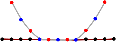
Figure 1: If we color the nodes of a unique shortest path with alternating colors, then its nodes will contribute discrepancy $0$, $+1$, or $-1$ to all unique shortest paths that intersect it.

Summing together these two parts, we obtain a bound of $\widetilde{O}(n^{1/4})$ on discrepancy, which holds with high probability. We can translate this to a bound on hereditary discrepancy using the fact that consistency is a hereditary property of path systems.

Lower Bound Techniques. For lower bounds, we apply the trace bound of [CL00] on hereditary discrepancy together with an explicit graph construction [BH23] that was recently proposed as a lower bound against hopsets in graphs. An (exact) hopset of a graph $G$ with hopbound $\beta$ is a small set of additional edges $H$ in the distance closure of $G$, such that every pair of nodes has a shortest path in $G\cup H$ containing at most $\beta$ edges.

Until recently, the state-of-the-art hopset lower bounds were achieved using a point-line construction of Erdős [PA11], which had $n$ points and $n$ lines in $\mathbb{R}^{2}$ with each point staying on $\Theta(n^{1/3})$ lines and each line going through $\Theta(n^{1/3})$ points. This point-line system also implies tight lower bounds for the Szemerédi-Trotter theorem and the discrepancy of arrangements of lines in the plane [CL00], as well as the previous state-of-the-art lower bound on the discrepancy of unique shortest paths.

This point-line construction can be associated with a graph that possesses useful properties derived from geometry. If edges in this graph are weighted by Euclidean distance, then the paths in the graph corresponding to straight lines are unique shortest paths by design. On the other hand, two such shortest paths (along straight lines) only intersect at most once.

Recently, a construction in [BH23] obtained stronger hopset lower bounds with a different geometric graph construction, which still took place in $\mathbb{R}^{2}$ but allowed shortest paths to have multiple vertices/edges in common. We show that this construction can be repurposed to derive a stronger lower bound of $\Omega(n^{1/4})$ on vertex hereditary discrepancy, by applying the trace bound of [CL00]. Combined with our upper bounds, this substantially improves our understanding of the discrepancy of unique shortest paths.

The above upper and lower bounds are for general graphs. Naturally, one can ask if we have better bounds for special families of graphs. We further show that the lower bounds remain the same for two interesting families: planar graphs and bipartite graphs. The lower bound construction mentioned above is not planar, and so this requires some additional work. A natural attempt is to restore planarity by adding vertices to the construction wherever two edges cross. However, this comes at a cost of an increase in the number of vertices, and also with a potential danger of altering the shortest paths. In Section 5 we first show that the number of crossings is not too much higher than $n$. Then, by carefully changing the weights of the edges and by exploiting the geometric properties of the construction, we show that the topology and incidence of shortest paths are not altered. For bipartite graphs, although the vertex discrepancy can be made very low – by coloring the vertices on one side $+1$ and vertices on the other side $-1$ – the hereditary discrepancy can be as high as the general graph setting. Specifically, we show a 2-lift of any graph $G$ to a bipartite graph which essentially keeps the same hereditary discrepancy. Details can be found in Section 6.

2 Preliminaries

A path system is a pair $S=(V,\Pi)$ where $V$ is a ground set of nodes and $\Pi$ is a set of vertex sequences called paths. Each path may contain at most one instance of each node. We now formally define consistency, a structural property of unique shortest paths that will be useful.

Definition 3.

A path system $S=(V,\Pi)$ is consistent if no two paths in $S$ intersect, split apart, and then intersect again later. Formally:

• In the undirected setting, consistency means that for all $u,v\in V$ and all $\pi_{1},\pi_{2}\in\Pi$ such that $u,v\in\pi_{1}\cap\pi_{2}$, we have that $\pi_{1}[u,v]=\pi_{2}[u,v]$, i.e., the intersection of $\pi_{1}$ and $\pi_{2}$ is a contiguous subpath (subsequence) of $\pi_{1}$ and $\pi_{2}$.

• In the directed setting, consistency means that for all $u,v\in V$ and all $\pi_{1},\pi_{2}\in\Pi$ such that $u$ precedes $v$ in both $\pi_{1}$ and $\pi_{2}$, we have that $\pi_{1}[u,v]=\pi_{2}[u,v]$.

In every weighted graph for which all pairs shortest paths exist (i.e. no negative cycles), we can represent all-pairs shortest paths using a consistent path system. In particular, if all shortest paths are unique, then consistency is implied immediately.

We will investigate the combinatorial discrepancy of path systems $(V,\Pi)$. Usually, we will assume that $|V|=n$ and $|\Pi|$ is polynomial in $n$. We define a vertex coloring $\chi:V\mapsto\{-1,1\}$ and define the discrepancy of $\Pi$ as

$$\operatorname{disc}(\Pi)=\min_{\chi}\chi(\Pi),\,\quad\mbox{where }\chi(\Pi)=\max_{\pi\in\Pi}\left|\chi(\pi)\right|,\,\chi(\pi)=\sum_{v\in\pi}\chi(v).$$

Using a random coloring $\chi$, we can guarantee that for all paths $\pi\in\Pi$ [Cha00]:

$$|\chi(\pi)|\leq\sqrt{2|\pi|\ln(4|\Pi|)}.$$

This immediately provides a few observations.

Observation 2.1.

When $\Pi$ is a set of paths with size polynomial in $n$, then $\operatorname{disc}(\Pi)=O(\sqrt{n\log n})$. This bound is true even for paths that are possibly non-consistent.

Observation 2.2.

When the longest path in $\Pi$ has $D$ vertices we have $\operatorname{disc}(\Pi)=O(\sqrt{D\log n})$. Thus, for graphs that have a small diameter (e.g., small world graphs), the discrepancy of shortest paths is automatically small.

Hereditary discrepancy is a more robust measure of the complexity of a path system $(V,\Pi)$, defined as $\operatorname{herdisc}(\Pi)=\max_{Y\subseteq V}\operatorname{disc}(\Pi|_{Y})$, where $\Pi|_{Y}$ is the collection of sets of the form $\pi\cap Y$ with $\pi\in\Pi$. Clearly, $\operatorname{herdisc}(\Pi)\geq\operatorname{disc}(\Pi)$. Sometimes the discrepancy of a set system may be small while the hereditary discrepancy is large [Cha00]. Thus in the literature, we often talk about lower bounds on the hereditary discrepancy.

Now that we have defined vertex and edge (hereditary) discrepancy, one may wonder if there is an underlying relationship between vertex and edge (hereditary) discrepancy since they share the same bounds in most scenarios as presented in Table 1. The following observation shows that vertex discrepancy directly implies bounds on edge discrepancy.

Observation 2.3.

Denote by $\operatorname{disc}(n)$ (and $\operatorname{herdisc}(n)$) the maximum discrepancy (minimum hereditary discrepancy, respectively) of a consistent path system of a (undirected or directed) graph of $n$ vertices. We have that

1. Let $g(x)$ be a non-decreasing function. If $\textnormal{herdisc}_{v}(n)\geq g(n)$, then $\textnormal{herdisc}_{e}(n)\geq g(n/2)$.

2. Let $f(x)$ be a non-decreasing function. If $\textnormal{disc}_{v}(n)\leq f(n)$, then $\textnormal{disc}_{e}(m)\leq f(m)$.

The proof of 2.3 is deferred to Appendix E. We also use some technical tools from discrepancy theory and statistics. For details please refer to Appendix A.

3 General Graphs: Upper Bound Existential Proof

This section collects the existential proof of the upper bounds on vertex- and edge-discrepancy for consistent path systems in (possibly) directed graphs. Our approach uses Proposition A.1, which gives a discrepancy upper bound using the primal shatter function of a set system. This approach leads to the same upper bounds for undirected and directed graphs. In specifics, we show an upper bound of $\widetilde{O}(n^{1/4})$ holds for vertex discrepancy, while the edge discrepancy is at most $\widetilde{O}(m^{1/4})$. That is, we show an existential proof of Theorem 3 (on directed graphs) by this approach. Note that for undirected graphs, we have achieved better edge discrepancy bounds using explicit constructions (as shown in Section 4.3).

Consider a family of consistent paths $(V,\Pi)$. If a pair of vertices $u,v\in V$ appear on a path $\pi\in\Pi$, there is a unique set $R(u,v)$ which contains the set of vertices between $u,v$ (with $u,v$ inclusive) on the path $\pi$. Therefore, we define a set system $(V,\mathcal{R})$ where the ground set is the vertices $V$ of the graph, and, for each pair $u,v\in V$, we define the set $R(u,v)\in\mathcal{R}$ as before. The following argument holds for consistent path systems in both undirected and directed graphs, thus giving a proof of Theorem 3. See 3

Proof.

Let’s consider vertex discrepancy first, recall Definition 5, it is easy to verify that the primal shatter function for a consistent path system is $\pi_{\mathcal{R}}(s)=O(s^{2})$ – the intersection of any set $A$ of $s$ vertices with a range $R(u,v)$ will be defined by $A\cap R(x,y)$ with $x$ and $y$ being the first and last vertex on the path $\pi$ that defines $R(u,v)$ in a consistent path system. Since the size of the ground state (all vertices) is $n$, Proposition A.1 implies that the vertex discrepancy of the incident matrix for a family of consistent paths on a graph is at most $O(n^{1/4}\log^{5/4}n)$. The edge discrepancy follows the same pattern, only that the size of the ground state becomes $m=|E|$; therefore, we have the edge discrepancy is at most $O(m^{1/4}\log^{5/4}m)$.

Finally, to show the upper bound on hereditary discrepancy, we observe that for any subset $U\subseteq V$, we can define the system $\Pi[U]$ of the paths in $\Pi$ induced on the nodes in $U$. This path system $\Pi[U]$ will be consistent. Applying the above argument on $\Pi[U]$ will again give us an $O(n^{1/4}\log^{5/4}n)$ upper bound for the discrepancy of $\Pi[U]$, implying our desired vertex hereditary discrepancy upper bound. A similar argument achieves a edge hereditary discrepancy upper bound of $O(m^{1/4}\log^{5/4}m)$. ∎

Notice that for a sparse graph (i.e., $m=O(n)$) this matches the bound on vertex discrepancy, but for a dense graph (i.e., $m=\Theta(n^{2})$), the upper bound becomes $O(n^{1/2}\log^{5/4}n)$, which is no better than the upper bound by random coloring (2.1).

In the next section, we will present a constructive proof of the vertex discrepancy upper bound with an improvement on the logarithmic factors. Additionally, we will present a constructive proof for edge discrepancy of $\widetilde{O}(n^{1/4})$ for undirected graphs and DAG’s, which is a significant improvement over $\tilde{O}(m^{1/4})$, especially for dense graphs.

4 Undirected Graphs: Lower Bound and Explicit Colorings

We now discuss the main result (Theorem 2). We first show in Section 4.1 a hereditary discrepancy lower bound of $\Omega(n^{1/4})$ for both edge and vertex discrepancy in general undirected graphs. Then in Section 4.2 we present a vertex coloring achieving hereditary discrepancy of $\widetilde{O}(n^{1/4})$. Finally, we present an explicit edge coloring with the same hereditary discrepancy bound in Section 4.3.

4.1 Lower Bound

As suggested by 2.3, we focus on the vertex hereditary discrepancy, and our goal is to prove the following statement (Theorem 5). In Theorem 10, given later in Appendix C, we show that this theorem implies the same lower bound on (non-hereditary) vertex discrepancy as well.

Theorem 5.

There are examples of $n$-vertex undirected weighted graphs $G$ with a unique shortest path between each pair of vertices in which this system of shortest paths $\Pi$ has

$$\textnormal{herdisc}_{v}(\Pi)\geq\Omega(n^{1/4}).$$

To obtain the lower bound, we employ the new graph construction by [BH23], which shows that any exact hopset with $O(n)$ edges must have at least $\widetilde{\Omega}(n^{1/2})$ hop diameter. Despite seeming unrelated, this construction also sheds light on our problem. Another technique we use to show the hereditary discrepancy lower bound is the trace bound shown by [CL00] (and restated in Lemma A.2). In the following proof section, we first summarize the construction related to our objective, then show the calculation using the trace bound that leads to our lower bound.

Proof.

The key properties of the graph construction in [BH23] (see also Section 5.1) that we need can be summarized in the following lemma.

Lemma 4.1 (Lemma 1 of [BH23]).

For any $p=[1,n^{2}]$, there is an infinite family of $n$-node undirected weighted graphs $G=(V,E,w)$ and sets $\Pi$ of $p$ paths in $G$ such that

• $G$ has $\ell=\Theta\left(\frac{n}{p^{1/2}\log^{1/2}n}\right)$ layers. Each path in $\Pi$ starts in the first layer, ends in the last layer, and contains exactly one node in each layer.

• Each path in $\Pi$ is the unique shortest path between its endpoints in $G$.

• For any two nodes $u,v\in V$, there are at most $\frac{\ell}{h(u,v)}$ paths in $\Pi$ that contain both $u$ and $v$, where $h(u,v)$ is the distance between $u$ and $v$ in $G$ and $1\leq h(u,v)\leq\ell$.

We will make use of the shortest path vertex incidence matrix of this graph. Recall that hereditary discrepancy considers the sub-incidence matrix induced by columns corresponding to a set of vertices. We select the set of vertices occurring in the paths in $\Pi$, and show it leads to hereditary discrepancy at least $\Omega(n^{1/4})$. Specifically, take $A$ as the incidence matrix such that each row corresponds to one path in $\Pi$. $A$ has dimension $p\times n$ where $n$ is the number of vertices in $G$ and the $(i,j)$-th entry of $A$ is $1$ is the vertex $j$ is in the path $i$.

Now define $M=A^{T}A$. Recall that $\operatorname{tr}(M)$ is the number of $1$s in the matrix $A$. Since by construction, every path has length $\ell$, we have $\operatorname{tr}(M)=p\ell$. Furthermore, let $m_{ij}$ be the $(i,j)$-th element of matrix $M$, and observe that it is exactly the number of paths that contain vertices $i$ and $j$. (Note that $m_{ij}=m_{ji}$.) Additionally, $\operatorname{tr}(M^{2})$ is the number of length 4 closed paths in the bipartite graph representing the incidence matrix $A$. This implies that

$$\operatorname{tr}(M^{2})=\sum_{j=1}^{p}\sum_{u,v\in P_{j}}m_{u,v}=\sum_{j=1}^{p}\sum_{i=1}^{\ell}\sum_{\begin{subarray}{c}u,v\in P_{j},\\ h(u,v)=i\end{subarray}}m_{u,v}\leq\sum_{j=1}^{p}\sum_{i=1}^{\ell}\ell\cdot\frac{\ell}{i}\leq p\ell^{2}\log\ell.$$

By setting $p=n\log n$, it follows that $\ell=\Theta(\sqrt{n}/\log n)$ and $\operatorname{tr}(M)=p\ell=n^{3/2}$. So for large enough $n$, we have

$$\frac{n\cdot\operatorname{tr}(M^{2})}{(\operatorname{tr}(M))^{2}}\leq\frac{np\ell^{2}\log\ell}{p^{2}\ell^{2}}=\frac{n}{p}\cdot\log{\ell}=\frac{n(\log(n)/2-\log\log(n))}{n\log(n)}=\frac{1}{2}-\frac{\log\log(n)}{\log(n)}\leq\frac{1}{2}.$$

Let $c\in(0,1)$ be the constant implicit in Lemma A.2. Taking $c_{2}=c^{1/2}$, the trace bound gives us the desired bound:

$$\operatorname{herdisc}(A)\geq\frac{1}{4}\cdot c_{2}\sqrt{{\operatorname{tr}(M)}/{n}}=\frac{c_{2}}{4}\sqrt{\ell\log n}\geq\Omega(n^{1/4}).$$

∎

4.2 Vertex Discrepancy Upper Bound – Explicit Coloring

In this subsection, we will upper bound the discrepancy $\chi(\Pi)$ of a consistent path system $(V,\Pi)$ with $|V|=n$ and $|\Pi|=\textrm{poly}(n)$. This will immediately imply an upper bound for the hereditary vertex discrepancy of unique shortest paths in undirected graphs.

Theorem 6.

For a consistent path system $S=(V,\Pi)$ where $|V|=n$ and $|\Pi|=\textrm{poly}(n)$, there exists a labeling $\chi$ such that $\chi(\Pi)=O(n^{1/4}\log^{1/2}n).$ Consequently, every $n$-vertex undirected graph has hereditary vertex discrepancy $O(n^{1/4}\log^{1/2}n)$.

Let $S=(V,\Pi)$ be a consistent path system with $|V|=n$ and $|\Pi|=\textrm{poly}(n)$. As the first step towards constructing our labeling $\chi:V\mapsto\{-1,1\}$, we will construct a collection of paths $\Pi^{\prime}$ on $V$ that will have a useful covering property over the paths in $\Pi$.

Constructing path cover $\Pi^{\prime}$. Initially, we let $\Pi^{\prime}=\emptyset$. We define $V^{\prime}$ to be the set of all nodes in $V$ belonging to a path in $\Pi^{\prime}$, i.e., $V^{\prime}:=\bigcup_{\pi^{\prime}\in\Pi^{\prime}}\pi^{\prime}.$ While $\left|\pi\setminus V^{\prime}\right|\geq n^{1/2}$ for some $\pi\in\Pi$, find a (possibly non-contiguous) subpath of $\pi$ of length $n^{1/2}$ that is vertex-disjoint from all paths in $\Pi^{\prime}$. Formally, find a subpath $\pi^{\prime}\subseteq\pi$ such that $|\pi^{\prime}|=n^{1/2}$ and $\pi^{\prime}\cap V^{\prime}=\emptyset$. Add path $\pi^{\prime}$ to path cover $\Pi^{\prime}$ and update $V^{\prime}$. Repeatedly add paths to path cover $\Pi^{\prime}$ in this manner until $|\pi\setminus V^{\prime}|<n^{1/2}$ for all $\pi\in\Pi$.

Proposition 4.2.

Path cover $\Pi^{\prime}$ satisfies the following properties:

1. for all $\pi\in\Pi^{\prime}$, $|\pi|=n^{1/2}$,

2. the number of paths in $\Pi^{\prime}$ is $|\Pi^{\prime}|\leq n^{1/2}$,

3. (Disjointness Property) The paths in $\Pi^{\prime}$ are pairwise vertex-disjoint,

4. (Covering Property) For all $\pi\in\Pi$, the number of nodes in $\pi$ that do not lie in any path in path cover $\Pi^{\prime}$ is at most $n^{1/2}$. Formally, let $V^{\prime}=\cup_{\pi^{\prime}\in\Pi^{\prime}}\pi^{\prime}$. Then $\forall\pi\in\Pi,\left|\pi\setminus V^{\prime}\right|\leq n^{1/2},$

5. (Consistency Property) For all $\pi\in\Pi$ and $\pi^{\prime}\in\Pi^{\prime}$, the intersection $\pi\cap\pi^{\prime}$ is a (possibly empty) contiguous subpath of $\pi^{\prime}$.

Proof.

Properties 1, 3, and 4 follows from the construction of $\Pi^{\prime}$. Property 2 follows from Properties 1 and 3 and the fact that $|V|=n$. The Consistency Property of $\Pi^{\prime}$ is inherited from the consistency of path system $S$. Specifically, by the construction of $\Pi^{\prime}$, path $\pi^{\prime}\in\Pi^{\prime}$ is a subpath of a path $\pi^{\prime\prime}\in\Pi$. Recall that by the consistency of path system $S$, the intersection $\pi\cap\pi^{\prime\prime}$ is a (possibly empty) contiguous subpath of $\pi^{\prime\prime}$. Then $\pi\cap\pi^{\prime}$ is a contiguous subpath of $\pi^{\prime}$ since $\pi^{\prime}\subseteq\pi^{\prime\prime}$. This concludes the proof. ∎

Constructing labeling $\chi$. Let $\pi^{\prime}=(v_{1},\dots,v_{k})\in\Pi^{\prime}$ be a path in our path cover. We will label the nodes of $\pi^{\prime}$ using the following random process. With probability $1/2$ we define $\chi:\pi^{\prime}\mapsto\{-1,1\}$ to be

$$\chi(v_{i})=\begin{cases}1&i\equiv 0\mod 2\text{ and }i\in[1,k]\\ -1&i\equiv 1\mod 2\text{ and }i\in[1,k]\end{cases},$$

and with probability $1/2$ we define $\chi:\pi^{\prime}\mapsto\{-1,1\}$ to be

$$\chi(v_{i})=\begin{cases}-1&i\equiv 0\mod 2\text{ and }i\in[1,k]\\ 1&i\equiv 1\mod 2\text{ and }i\in[1,k]\end{cases}.$$

The labels of consecutive nodes in $\pi^{\prime}$ alternate between $1$ and $-1$, with vertex $v_{1}$ taking labels $1$ and $-1$ with equal probability. Since the paths in path cover $\Pi^{\prime}$ are pairwise vertex-disjoint, the labeling $\chi$ is well-defined over $V^{\prime}:=\cup_{\pi^{\prime}\in\Pi^{\prime}}\pi^{\prime}$. We choose a random labeling for all nodes in $V\setminus V^{\prime}$, i.e., we independently label each node $v\in V\setminus V^{\prime}$ with $\chi(v)=-1$ with probability $1/2$ and $\chi(v)=1$ with probability $1/2$. An illustration can be found in Figure 2.

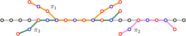
Figure 2: In this figure, paths $\pi_{1},\pi_{2},\pi_{3}\in\Pi^{\prime}$ from the path cover are intersecting a path $\pi\in\Pi$. Paths in the path cover are pairwise vertex-disjoint, and each path in the cover contributes discrepancy $0$, $-1$, or $+1$ to $\pi$.

Bounding the discrepancy $\chi(\Pi)$. Fix a path $\pi\in\Pi$. We will show that $\left|\sum_{v\in\pi}\chi(v)\right|=O(n^{1/4}\log^{1/2}n)$ with high probability. Theorem 6 would follow as $|\Pi|=\textrm{poly}(n)$.

Proposition 4.3.

For each path $\pi^{\prime}$ in path cover $\Pi^{\prime}$,

$$\left|\sum_{v\in\pi\cap\pi^{\prime}}\chi(v)\right|\in\{-1,0,1\}.$$

If $|\pi\cap\pi^{\prime}|\equiv 0\mod 2$, then $\left|\sum_{v\in\pi\cap\pi^{\prime}}\chi(v)\right|=0$. Moreover,

$$\Pr\left[\left|\sum_{v\in\pi\cap\pi^{\prime}}\chi(v)\right|=-1\right]=\Pr\left[\left|\sum_{v\in\pi\cap\pi^{\prime}}\chi(v)\right|=1\right].$$

Proof.

By the Consistency Property of $\Pi^{\prime}$ (as proven in Proposition 4.2), path $\pi\cap\pi^{\prime}$ is a (possibly empty) contiguous subpath of $\pi^{\prime}$. Then since consecutive nodes in $\pi^{\prime}$ alternate between $-1$ and $1$, it follows that $\left|\sum_{v\in\pi\cap\pi^{\prime}}\chi(v)\right|\in\{-1,0,1\}$.

Now note that $\left|\sum_{v\in\pi\cap\pi^{\prime}}\chi(v)\right|\neq 0$ iff $|\pi\cap\pi^{\prime}|$ is odd. Moreover, the first vertex of $\pi\cap\pi^{\prime}$ takes labels $1$ and $-1$ with equal probability. This concludes the proof of Proposition 4.3. ∎

We are now ready to bound the discrepancy of $\pi$.

Proposition 4.4.

With high probability, $\chi(\pi)=O(n^{1/4}\log^{1/2}n)$.

Proof.

We partition the nodes of $\pi$ into two sources of discrepancy that we will bound separately. Let $V^{\prime}:=\cup_{\pi^{\prime}\in\Pi^{\prime}}\pi^{\prime}$.

Discrepancy of $\pi\cap V^{\prime}$. For each path $\pi^{\prime}\in\Pi^{\prime}$, let $X_{\pi^{\prime}}$ be the random variable defined as

$$X_{\pi^{\prime}}:=\left|\sum_{v\in\pi\cap\pi^{\prime}}\chi(v)\right|.$$

We can restate the discrepancy of $\pi\cap V^{\prime}$ as

$$\left|\sum_{v\in\pi\cap V^{\prime}}\chi(v)\right|=\sum_{\pi^{\prime}\in\Pi^{\prime}}X_{\pi^{\prime}}.$$

By Proposition 4.3, if $|\pi\cap\pi^{\prime}|\equiv 0\mod 2$, then $X_{\pi^{\prime}}=0$, so we may assume without any loss of generality that $|\pi\cap\pi^{\prime}|$ is odd for all $\pi^{\prime}\in\Pi^{\prime}$. In this case, $\Pr\left[X_{\pi^{\prime}}=-1\right]=\Pr\left[X_{\pi^{\prime}}=1\right]=1/2,$ implying that $\mathbb{E}[\sum_{\pi^{\prime}\in\Pi^{\prime}}X_{\pi^{\prime}}]=0$. Then by Proposition 4.2 and Chernoff, it follows that for any constant $c\geq 1$,

$$\Pr\left[\sum_{\pi^{\prime}\in\Pi^{\prime}}X_{\pi^{\prime}}\geq c\cdot n^{1/4}\log^{1/2}n\right]\leq e^{-c^{2}\frac{n^{1/2}\log n}{2|\Pi^{\prime}|}}\leq e^{-c^{2}/(2\cdot\log(n))}=n^{-c^{2}/2}.$$

Discrepancy of $\pi\setminus V^{\prime}$. Note that by the Covering Property of the path cover (as proven in Proposition 4.2), $|\pi\setminus V^{\prime}|\leq n^{1/2}$. Moreover, the nodes in $V\setminus V^{\prime}$ are labeled independently at random, implying that $\mathbb{E}[\sum_{v\in\pi\setminus V^{\prime}}\chi(v)]=0$. Then we may apply a Chernoff bound to argue that for any constant $c\geq 1$,

$$\Pr\left[\left|\sum_{v\in\pi\setminus V^{\prime}}\chi(v)\right|\geq c\cdot n^{1/4}\log^{1/2}n\right]\leq e^{-c^{2}\frac{n^{1/2}\log n}{2|\pi\setminus V^{\prime}|}}\leq e^{-c^{2}/(2\cdot\log(n))}=n^{-c^{2}/2}.$$

We have shown that with high probability, the discrepancy of our labeling is $O(n^{1/4}\log^{1/2}n)$ for $\pi\cap V^{\prime}$ and $O(n^{1/4}\log^{1/2}n)$ for $\pi\setminus V^{\prime}$, so we conclude that the total discrepancy of $\pi$ is $O(n^{1/4}\log^{1/2}n)$, completing the proof of Proposition 4.4. ∎

Extending to hereditary discrepancy. Let $A$ be the vertex incidence matrix of a path system $S=(V,\Pi)$ on $n$ nodes, and let $A_{Y}$ be the submatrix of $A$ obtained by taking all of its rows but only a subset $Y$ of its columns. Then there exists a subset $V_{Y}\subseteq V$ of the nodes in $V$ such that $A_{Y}$ is the vertex incidence matrix of the path system $S[V_{Y}]$ (path system $S$ induced on $V_{Y}$). Moreover, if path system $S$ is consistent, then $S[V_{Y}]$ is also consistent. Then we may apply our explicit vertex discrepancy upper bound to $S[V_{Y}]$. We conclude that the hereditary vertex discrepancy of $S$ is $O(n^{1/4}\log^{1/2}n)$.

4.3 Edge Discrepancy Upper Bound – Explicit Coloring

By Proposition A.1 and the discussion in Section 3, the edge discrepancy of a (possibly directed) graph on $m$ edges is $O(m^{1/4}\log^{5/4}m)$. However, in the case of undirected graphs and DAGs, we can improve the edge discrepancy to $O(n^{1/4}\log^{1/2}n)$, where $n$ is the number of vertices in the graph, by modifying the explicit construction for vertex discrepancy in Section 4.2. Our proof strategy will follow the same framework as the explicit construction for vertex discrepancy, but with some added complications in the construction and analysis.

We first introduce some new notation that will be useful in this section. Given a path $\pi$ and nodes $u,v\in\pi$, we say that $u<_{\pi}v$ if $u$ occurs before $v$ on path $\pi$. Additionally, given a path system $S=(V,\Pi)$, we define the edge set $E\subseteq V\times V$ of the path system as the set of all pairs of nodes $u,v\in V$ that appear consecutively in some path in $\Pi$. Likewise, for any path $\pi$ over the vertex set $V$, we define the edge set of $\pi$, $E(\pi)\subseteq\pi\times\pi$, as the set of all pairs of nodes $u,v\in\pi$ such that $u,v$ appear consecutively in $\pi$ and $(u,v)\in E$. Note that if path system $S$ corresponds to paths in a graph $G$, then $E$ will be precisely the edge set of $G$.

Recall that we wish to construct an edge labeling $\chi:E\mapsto\{-1,1\}$ so that

$$\chi(\Pi)=\max_{\pi\in\Pi}\left|\sum_{e\in E(\pi)}\chi(e)\right|$$

is minimized. We will upper bound the discrepancy $\chi(\Pi)$ of consistent path systems such that $|V|=n$ and $|\Pi|=\textrm{ poly}(n)$. This will immediately imply an upper bound on the edge discrepancy of unique shortest paths in undirected graphs.

Theorem 7.

For all consistent path systems $S=(V,\Pi)$ where $|V|=n$ and $|\Pi|=\textrm{poly}(n)$, there exists a labeling $\chi:E\to\{-1,1\}$ such that

$$\chi(\Pi)=O(n^{1/4}\log^{1/2}n).$$

Consequently, every $n$-vertex undirected graph has hereditary edge discrepancy $O(n^{1/4}\log^{1/2}n)$.

Let $S=(V,\Pi)$ be a consistent path system with $|V|=n$ and $|\Pi|=\textrm{poly}(n)$. As the first step towards constructing our labeling $\chi:E\mapsto\{-1,1\}$, we will construct a collection of paths $\Pi^{\prime}$ on $V$ that will have a useful covering property over the paths in $\Pi$.

Constructing path cover $\Pi^{\prime}$.

Initially, we let $\Pi^{\prime}=\emptyset$. We define $V^{\prime}$ to be the set of all nodes in $V$ belonging to a path in $\Pi^{\prime}$, i.e.,

$$V^{\prime}:=\bigcup_{\pi^{\prime}\in\Pi^{\prime}}\pi^{\prime}.$$

While there exists a path $\pi\in\Pi$ such that $\left|\pi\setminus V^{\prime}\right|\geq n^{1/2}$, find a (possibly non-contiguous) subpath of $\pi$ of length $n^{1/2}$ that is vertex-disjoint from all paths in $\Pi^{\prime}$. Specifically, let $\pi^{\prime}\subseteq\pi$ be a (possibly non-contiguous) subpath of $\pi$ containing exactly the first $n^{1/2}$ nodes in $\pi\setminus V^{\prime}$. Add path $\pi^{\prime}$ to path cover $\Pi^{\prime}$ and update $V^{\prime}$. Repeatedly add paths to path cover $\Pi^{\prime}$ in this manner until $|\pi\setminus V^{\prime}|<n^{1/2}$ for all $\pi\in\Pi$.

Note that our path cover $\Pi^{\prime}$ is very similar to the path cover used in the explicit vertex discrepancy upper bound. Indeed, path cover $\Pi^{\prime}$ inherits all properties of the path cover defined in Subsection 4.2. The key difference here is that we require subpaths $\pi^{\prime}\subseteq\pi$ in $\Pi^{\prime}$ to contain the first $n^{1/2}$ nodes in $\pi\setminus V^{\prime}$. This will imply an additional property of our path cover, which we call the No Repeats Property.

Figure 3: In this figure, paths $\pi_{1},\pi_{2}\in\Pi^{\prime}$ are intersecting a path $\pi\in\Pi$. This arrangement of paths is forbidden by the No Repeats Property of Proposition 4.5.

Proposition 4.5.

Path cover $\Pi^{\prime}$ satisfies all properties of Proposition 4.2, as well as the following additional properties:

• (Edge Covering Property) For all $\pi\in\Pi$, the number of edges in $\pi$ that are not incident to any node lying in a path in path cover $\Pi^{\prime}$ is at most $n^{1/2}$. Formally, let $V^{\prime}=\cup_{\pi^{\prime}\in\Pi^{\prime}}\pi^{\prime}$. For all $\pi\in\Pi$,

  $$\left|\{(u,v)\in E(\pi)\mid u\not\in V^{\prime}\text{ and }v\not\in V^{\prime}\}\right|\leq n^{1/2},$$

• (No Repeats Property) For all paths $\pi\in\Pi$, $\pi_{1},\pi_{2}\in\Pi^{\prime}$, and nodes $v_{1},v_{2},v_{3},v_{4}\in\pi$ such that $v_{1},v_{3}\in\pi_{1}$ and $v_{2},v_{4}\in\pi_{2}$, the following ordering of the vertices in $\Pi$ is impossible:

  $$v_{1}<_{\pi}v_{2}<_{\pi}v_{3}<_{\pi}v_{4},$$

  where $x<_{\pi}y$ indicates that node $x$ occurs in $\pi$ before node $y$.

Proof.

All properties from Proposition 4.2 follow from an identical argument as in the original proof. The Edge Covering Property follows immediately from the Covering Property of Proposition 4.2. What remains is to prove the No Repeats Property.

Suppose for the sake of contradiction that there exist paths $\pi\in\Pi$, $\pi_{1},\pi_{2}\in\Pi^{\prime}$, and nodes $v_{1},v_{2},v_{3},v_{4}\in\pi$ such that $v_{1},v_{3}\in\pi_{1}$ and $v_{2},v_{4}\in\pi_{2}$, where $v_{1}<_{\pi}v_{2}<_{\pi}v_{3}<_{\pi}v_{4}$. We will assume that path $\pi_{1}$ was added to $\Pi^{\prime}$ before path $\pi_{2}$ (the case where $\pi_{2}$ was added to $\Pi^{\prime}$ first is symmetric). By the construction of $\Pi^{\prime}$, path $\pi_{1}\in\Pi^{\prime}$ is a (possibly non-contiguous) subpath of a path $\pi_{1}^{\prime\prime}\in\Pi$ that it was constructed from. Additionally, by the consistency of the path system $S$, the intersection $\pi\cap\pi_{1}^{\prime\prime}$ is a contiguous subpath of $\pi$. Then $v_{2}\in\pi\cap\pi_{1}^{\prime\prime}$, and specifically, $v_{2}\in\pi_{1}^{\prime\prime}$.

We assumed that $v_{2}\in\pi_{2}$, which implies that $v_{2}\not\in\pi_{1}$, since paths in $\Pi^{\prime}$ are pairwise vertex-disjoint. Since path $\pi_{1}$ was added to $\Pi^{\prime}$ before path $\pi_{2}$, this means that when $\pi_{1}$ was added to $\Pi^{\prime}$, node $v_{2}$ did not belong to any path in $\Pi^{\prime}$ (i.e., $v_{2}$ was not in $V^{\prime}$). Recall that in our construction of $\Pi^{\prime}$, we constructed subpath $\pi_{1}\subseteq\pi_{1}^{\prime\prime}$ so that it contained exactly the first $n^{1/2}$ nodes in $\pi_{1}^{\prime\prime}\setminus V^{\prime}$. However, $v_{2}\not\in\pi_{1}$, but $v_{3}\in\pi_{1}$, and $v_{2}$ comes before $v_{3}$ in $\pi_{1}^{\prime\prime}$. This contradicts our construction of path $\pi_{1}$ in path cover $\Pi^{\prime}$. ∎

The Edge Covering Property of Proposition 4.5 does not provide any upper bound on the number of edges $(u,v)\in E(\pi)$ that are incident to one or more vertices in $V^{\prime}$. This is the main source of complications in the analysis of our edge discrepancy upper bound.

Constructing labeling $\chi$.

Let $\pi^{\prime}\in\Pi^{\prime}$ be a path of length $k$ in our path cover. Let $e_{1},\dots,e_{k}\in E(\pi^{\prime})$ be the edges in $\pi^{\prime}$ listed in the order they appear in $\pi^{\prime}$. Note that since $\pi^{\prime}$ is a possibly non-contiguous subpath of a path in $\Pi$, pairs of nodes $u,v\in V$ that appear consecutively in $\pi$ do not necessarily correspond to edges in edge set $E$.

We will label the edges in $E(\pi^{\prime})$ using the following random process. With probability $1/2$ we define $\chi:E(\pi^{\prime})\mapsto\{-1,1\}$ to be

$$\chi(e_{i})=\begin{cases}1&i\equiv 0\mod 2\text{ and }i\in[1,k]\\ -1&i\equiv 1\mod 2\text{ and }i\in[1,k]\end{cases},$$

and with probability $1/2$ we define $\chi:E(\pi^{\prime})\mapsto\{-1,1\}$ to be

$$\chi(e_{i})=\begin{cases}-1&i\equiv 0\mod 2\text{ and }i\in[1,k]\\ 1&i\equiv 1\mod 2\text{ and }i\in[1,k]\end{cases}.$$

Note that the labels of consecutive edges $e_{i},e_{i+1}$ in $\pi^{\prime}$ alternate between $1$ and $-1$, with edge $e_{1}$ taking labels $1$ and $-1$ with equal probability.

Since the paths in path cover $\Pi^{\prime}$ are pairwise vertex-disjoint, the labeling $\chi$ is well-defined over $E^{\prime}:=\cup_{\pi^{\prime}\in\Pi^{\prime}}E(\pi^{\prime})$. We take a random labeling for all edges in $E\setminus E^{\prime}$, i.e., we independently label each edge $e\in E\setminus E^{\prime}$ with $\chi(e)=-1$ with probability $1/2$ and $\chi(e)=1$ with probability $1/2$.

Bounding the discrepancy $\phi$.

Fix a path $\pi:=\pi[s,t]\in\Pi$. We will show that

$$\left|\sum_{e\in E(\pi)}\chi(e)\right|=O(n^{1/4}\log^{1/2}n)$$

with high probability. This will complete the proof of Lemma 7 since $|\Pi|=\textrm{poly}(n)$. The proof of the following proposition follows from an argument identical to Proposition 4.3 and hence omitted.

Proposition 4.6.

For each path $\pi^{\prime}$ in path cover $\Pi^{\prime}$,

$$\left|\sum_{e\in E(\pi)\cap E(\pi^{\prime})}\chi(e)\right|\in\{-1,0,1\}.$$

If $|E(\pi)\cap E(\pi^{\prime})|\equiv 0\mod 2$, then $\left|\sum_{e\in E(\pi)\cap E(\pi^{\prime})}\chi(e)\right|=0$. Moreover,

$$\Pr\left[\left|\sum_{e\in E(\pi)\cap E(\pi^{\prime})}\chi(e)\right|=-1\right]=\Pr\left[\left|\sum_{e\in E(\pi)\cap E(\pi^{\prime})}\chi(e)\right|=1\right].$$

We are now ready to bound the edge discrepancy of $\pi$. Define

$$V^{\prime}:=\bigcup_{\pi^{\prime}\in\Pi^{\prime}}\pi^{\prime}\quad\text{and}\quad E^{\prime}:=\bigcup_{\pi^{\prime}\in\Pi^{\prime}}E(\pi^{\prime}).$$

We partition the edges of the path $\pi$ into three sources of discrepancy that we will bound separately. Specifically, we split $E(\pi)\subseteq\pi\times\pi$ into the following sets $E_{1},E_{2},E_{3}$:

• $E_{1}:=E(\pi)\cap E^{\prime}$,

• $E_{2}:=E(\pi)\cap((V\setminus V^{\prime})\times(V\setminus V^{\prime}))$, and

• $E_{3}:=E(\pi)\setminus(E_{1}\cup E_{2})$.

Sets $E_{1}$ and $E_{2}$ roughly correspond to the two sources of discrepancy considered in the vertex discrepancy upper bound, while set $E_{3}$ corresponds to a new source of discrepancy that will require new arguments to bound. We begin with set $E_{1}$.

Proposition 4.7 (Discrepancy of $E_{1}$).

With high probability, $\left|\sum_{e\in E_{1}}\chi(e)\right|=O(n^{1/4}\log^{1/2}n)$.

Proof.

The proposition follow from an argument similar to Proposition 4.4. For each path $\pi^{\prime}\in\Pi^{\prime}$, let $X_{\pi^{\prime}}$ be the random variable defined as

$$X_{\pi^{\prime}}:=\left|\sum_{e\in E(\pi)\cap E(\pi^{\prime})}\chi(e)\right|.$$

We can restate the discrepancy of $E_{1}$ as

$$\left|\sum_{e\in E_{1}}\chi(e)\right|=\sum_{\pi^{\prime}\in\Pi^{\prime}}X_{\pi^{\prime}}.$$

By Proposition 4.6, if $|E(\pi)\cap E(\pi^{\prime})|\equiv 0\mod 2$, then $X_{\pi^{\prime}}=0$, so without any loss of generality, we may assume that $|E(\pi)\cap E(\pi^{\prime})|$ is odd for all $\pi^{\prime}\in\Pi^{\prime}$. In this case,

$$\Pr\left[X_{\pi^{\prime}}=-1\right]=\Pr\left[X_{\pi^{\prime}}=1\right]=1/2,$$

implying that $\mathbb{E}[\sum_{\pi^{\prime}\in\Pi^{\prime}}X_{\pi^{\prime}}]=0$. Then by Proposition 4.5 and the Chernoff bound, it follows that for any constant $c\geq 1$,

$$\Pr\left[\sum_{\pi^{\prime}\in\Pi^{\prime}}X_{\pi^{\prime}}\geq c\cdot n^{1/4}\log^{1/2}n\right]\leq e^{-c^{2}\frac{n^{1/2}\log n}{2|\Pi^{\prime}|}}\leq e^{-c^{2}/2\cdot\log n}\leq n^{-c^{2}/2}.$$

∎

We now bound the discrepancy of $E_{2}$.

Proposition 4.8 (Discrepancy of $E_{2}$).

With high probability, $\left|\sum_{e\in E_{2}}\chi(e)\right|=O(n^{1/4}\log^{1/2}n)$.

Proof.

The proposition follow from an argument similar to Proposition 4.4. Note that by the Edge Covering Property of the path cover (Proposition 4.5),

$$|E_{2}|=\left|\{(u,v)\in E(\pi)\mid u,v\not\in V^{\prime}\}\right|\leq n^{1/2}.$$

Moreover, the edges in $E\setminus E^{\prime}$ are labeled independently at random, so we may apply a Chernoff bound to argue that for any constant $c\geq 1$,

$$\Pr\left[\left|\sum_{e\in E_{2}}\chi(e)\right|\geq c\cdot n^{1/4}\log^{1/2}n\right]\leq e^{-c^{2}\frac{n^{1/2}\log n}{2|E_{2}|}}\leq e^{-c^{2}/2\cdot\log n}\leq n^{-c^{2}/2}.$$

completing the proof. ∎

Proposition 4.9 ( Discrepancy of $E_{3}$).

With high probability, $\left|\sum_{e\in E_{3}}\chi(e)\right|=O(n^{1/4}\log^{1/2}n)$.

Proof.

Let

$$k:=\left|\{\pi^{\prime}\in\Pi^{\prime}\mid\pi\cap\pi^{\prime}\neq\emptyset\}\right|$$

denote the number of paths in our path cover that intersect $\pi$. We define a function $f:\mathbb{Z}_{\geq 0}\mapsto\mathbb{Z}_{\geq 0}$ such that $f(\phi)$ equals the largest possible value of $|E_{3}|$ when $\phi=k$. Note that $f$ is well-defined since $0\leq|E_{3}|\leq|E|$. We will prove that $f(\phi)\leq 4\phi,$ by recursively decomposing path $\pi$. When $\phi=1$, there is only one path $\pi^{\prime}\in\Pi^{\prime}$ that intersects $\pi$. Then the only edges in $E_{3}$ are of the form

$$E(\pi)\cap((V^{\prime}\times(V\setminus V^{\prime}))\cup((V\setminus V^{\prime})\times V^{\prime}))=E(\pi)\cap((\pi^{\prime}\times(V\setminus\pi^{\prime}))\cup((V\setminus\pi^{\prime})\times\pi^{\prime})).$$

By the Consistency Property of Proposition 4.5, path $\pi^{\prime}$ can intersect $\pi$ and then split apart at most once. Then

$$f(1)=|E_{3}|=|E(\pi)\cap((\pi^{\prime}\times(V\setminus\pi^{\prime}))\cup((V\setminus\pi^{\prime})\times\pi^{\prime}))|\leq 2.$$

When $\phi>1$, we will split our analysis into the two cases:

• Case 1. There exists paths $\pi_{1}^{\prime},\pi_{2}^{\prime}\in\Pi^{\prime}$ and nodes $v_{1},v_{2},v_{3}\in\pi$ such that $v_{1},v_{3}\in\pi_{1}^{\prime}$ and $v_{2}\in\pi_{2}^{\prime}$ and $v_{1}<_{\pi}v_{2}<_{\pi}v_{3}$. In this case, we can assume without any loss of generality that $\pi[v_{1},v_{3}]\cap\pi_{1}^{\prime}=\{v_{1},v_{3}\}$ (e.g., by choosing $v_{1},v_{3}$ so that this equality holds). Let $x$ be the node immediately following $v_{1}$ in $\pi$, and let $y$ be the node immediately preceding $v_{3}$ in $\pi$. Recall that $s$ is the first node of $\pi$ and $t$ is the last node of $\pi$. It will be useful for the analysis to split $\pi$ into three subpaths:

  $$\pi=\pi[s,v_{1}]\circ\pi[x,y]\circ\pi[v_{3},t],$$

  where $\circ$ denotes the concatenation operation. Let

  $$\phi_{1}:=|\{\pi^{\prime}\in\Pi^{\prime}\mid\pi[x,y]\cap\pi^{\prime}\neq\emptyset\}|\text{\qquad and \qquad}\phi_{2}:=|\{\pi^{\prime}\in\Pi^{\prime}\mid(\pi[s,v_{1}]\circ\pi[v_{3},t])\cap\pi^{\prime}\neq\emptyset\}|.$$

  We claim that $\phi_{1}<\phi$, $\phi_{2}<\phi$, and $\phi_{1}+\phi_{2}=\phi$. We will use these facts to establish a recurrence relation for $f$. By our assumption that $\pi[v_{1},v_{3}]\cap\pi_{1}^{\prime}=\{v_{1},v_{3}\}$, it follows that $\pi[x,y]\cap\pi_{1}^{\prime}=\emptyset$, and so $\phi_{1}<\phi$. Likewise, by the No Repeats Property of Proposition 4.5,

  $$(\pi[s,v_{1}]\circ\pi[v_{3},t])\cap\pi_{2}^{\prime}=\emptyset,$$

  so $\phi_{2}<\phi$. Finally, observe that more generally, if there exists a path $\pi^{\prime}\in\Pi^{\prime}$ such that $\pi^{\prime}\cap\pi[x,y]\neq\emptyset$ and $\pi^{\prime}\cap(\pi[s,v_{1}]\circ\pi[v_{3},t])\neq\emptyset$, then the No Repeats Property of Proposition 4.5 is violated. We conclude that $\phi_{1}+\phi_{2}=\phi$.

  Now $|E_{3}|$ can be upper bounded by the following inequality:

  $$|E_{3}|\leq|E_{3}\cap E(\pi[x,y])|+|E_{3}\cap E(\pi[s,v_{1}]\circ\pi[v_{3},t])|+2.$$

  Then using the observations about $\phi_{1},\phi_{2}$, and $\phi$ in the previous paragraph, we obtain the following recurrence for $f$:

  $$f(\phi)\leq f(\phi_{1})+f(\phi_{2})+2=f(i)+f(\phi-i)+2,$$

  where $0<i<\phi$.

• Case 2. There exists a path $\pi^{\prime}\in\Pi^{\prime}$ and $v_{1},v_{2}\in\pi$ such that $\pi\cap\pi^{\prime}=\pi[v_{1},v_{2}]\cap V^{\prime}$. Let $x$ be the node immediately preceding $v_{1}$ in $\pi$, and let $y$ be the node immediately following $v_{2}$ in $\pi$. Again, we split $\pi$ into three subpaths:

  $$\pi[s,t]=\pi[s,x]\circ\pi[v_{1},v_{2}]\circ\pi[y,t].$$

  Let

  $$\phi_{1}:=|\{\pi^{\prime}\in\Pi^{\prime}\mid\pi[v_{1},v_{2}]\cap\pi^{\prime}\neq\emptyset\}|\text{\qquad and \qquad}\phi_{2}:=|\{\pi^{\prime}\in\Pi^{\prime}\mid(\pi[s,x]\circ\pi[y,t])\cap\pi^{\prime}\neq\emptyset\}|.$$

  By our assumption in Case 2, it follows that $\phi_{1}=1$ and $\phi_{2}=\phi-1$. Since $|E_{3}|$ can be upper bounded by the inequality

  $$|E_{3}|\leq|E_{3}\cap E(\pi[v_{1},v_{2}])|+|E_{3}\cap E(\pi[s,x]\circ\pi[y,t])|+2,$$

  we immediately obtain the recurrence

  $$f(\phi)\leq f(\phi_{1})+f(\phi_{2})+2\leq f(1)+f(\phi-1)+2.$$

Taking our results from Case 1 and Case 2 together, we obtain the recurrence relation

$$f(\phi)\leq\begin{cases}\max\left\{f(i)+f(\phi-i)+2,\text{ }f(1)+f(\phi-1)+2\right\}&\phi>1\text{ and }1<i<\phi\\ 2&\phi=1\end{cases}$$

Applying this recurrence $\leq\phi$ times, we find that

$$f(\phi)\leq\phi\cdot f(1)+2\phi\leq 4\phi.$$

Finally, since $k\leq|\Pi^{\prime}|\leq n^{1/2}$ and we defined $f$ so that $f(k)$ equals the largest possible value of $|E_{3}|$, we conclude that

$$|E_{3}|\leq f(k)\leq f(n^{1/2})=O(n^{1/2}).$$

Since the edges in $E_{3}\subseteq E\setminus E^{\prime}$ are labeled independently at random, we may apply a Chernoff bound as in Proposition 4.8 to argue that $\chi(E_{3})=O(n^{1/4}\log^{1/2}n)$ with high probability. ∎

We have shown that with high probability, the discrepancy of our edge labeling is $O(n^{1/4}\log^{1/2}n)$ for $E_{1}$, $E_{2}$, and $E_{3}$, so we conclude that the total discrepancy of $\pi$ is $O(n^{1/4}\log^{1/2}n)$.

Extending to hereditary discrepancy.

Let $A$ be the edge incidence matrix of a path system $S=(V,\Pi)$ on $n$ nodes, and let $A_{Y}$ be the submatrix of $A$ obtained by taking all of its rows but only a subset $Y$ of its columns. We can rephrase the problem of bounding the discrepancy of $A_{Y}$ as the following edge coloring problem.

Let $E$ be the edge set of path system $S$, and let $E_{Y}\subseteq E$ be the set of edges in $E$ associated with the set of columns $Y$ in matrix $A$. Then bounding the discrepancy of $A_{Y}$ is equivalent to constructing an edge labeling $\chi:E_{Y}\mapsto\{-1,1\}$ so that $\chi(E_{Y}):=\max_{\pi\in\Pi}\left|\sum_{e\in E(\pi)\cap E_{Y}}\chi(e)\right|$ is minimized.

In this setting, for each $\pi\in\Pi$, we redefine $E(\pi)\subseteq\pi\times\pi$ to be the set of nodes $u,v\in\pi$ such that $u,v$ appear consecutively in $\pi$ and $(u,v)\in E_{Y}$. With this new definition of $E(\pi)$, we can construct an edge labeling $\chi$ using the exact same procedure described in this section. Indeed, we claim that this will yield the same discrepancy bound of $\chi(E_{Y})=O(n^{1/4}\log^{1/2}n)$.

The key observation needed to confirm this claim is that the consistency of path system $S$ extends to the setting where $S$ is restricted to edge set $E_{Y}$. Formally, for all paths $\pi_{1},\pi_{2}\in\Pi$, the set $E(\pi_{1})\cap E(\pi_{2})$ is a (possibly empty) contiguous subsequence of the edge sets $E(\pi_{1})$ and $E(\pi_{2})$. Using this observation in place of the notion of consistency, the discrepancy bounds on edge sets $E_{1},E_{2},E_{3}\subseteq E(\pi)$ follow from arguments identical to those of Propositions 4.7, 4.8, and 4.9. We conclude that the hereditary edge discrepancy of $S$ is $O(n^{1/4}\log^{1/2}n)$.

5 Planar Graphs

In this section, we will extend our hereditary vertex discrepancy lower bound for unique shortest paths in undirected graphs to the planar graph setting.

Theorem 8.

There exists an $n$-vertex undirected planar graph with hereditary vertex discrepancy at least $\Omega(n^{1/4}\log^{-3/2}n)$.

To prove this theorem, we will first give an abbreviated presentation of the graph construction in [BH23] that we used implicitly to obtain the $\Omega(n^{1/4})$ hereditary vertex discrepancy lower bound in Theorem 5. Then we will describe a simple procedure to make this graph planar and argue that the shortest path structure of this planarized graph remains unchanged.

5.1 Graph Construction of [BH23]

Take $n$ to be a large enough positive integer, and take $p=n\log n$. We will describe an $n$-node weighted undirected graph $G=(V,E,w)$ originally constructed in [BH23].

Vertex Set $V$.

We will use $\ell=\Theta\left(\frac{n^{1/2}}{\log n}\right)$ as a positive integer parameter for our construction. The graph $G$ we create will consist of $\ell$ layers, denoted as $L_{1},\dots,L_{\ell}$. Each layer will have $n/\ell$ nodes, arranged from $1$ to $n/\ell$. Initially, we will assign a tuple label $(i,j)$ to the $j$th node in the $L_{i}$ layer. We will interpret the node labeled $(i,j)$ as a point in $\mathbb{R}^{2}$ with integral coordinates. The vertex set $V$ of graph $G$ is made up of these $n$ nodes distributed across $\ell$ layers.

Next we will randomize the node labels in $V$. For each layer $L_{i}$, where $i$ ranges from 1 to $\ell$, we randomly and uniformly pick a real number in the interval $(0,1)$ and we call it $\psi_{i}$. After that, for each node in layer $L_{i}$ of the graph $G$ that is currently labeled $(i,j)$, we relabel it as

$$\left(i,j+\sum_{k=1}^{j}\psi_{k}\right).$$

These new labels for the nodes in $V$ are also treated as points in $\mathbb{R}^{2}$. We can imagine this process as adding a small epsilon of structured noise to the points corresponding to the nodes in the graph. The purpose of this noise is technical, but serves the purpose of achieving ‘symmetry breaking’ (see Section 2.4 of [BH23] for details).

Edge Set $E$.

All edges will be between subsequent layers $L_{i},L_{i+1}$ within $G$. It will be helpful to think of the edges in $G$ as directed from $L_{i}$ to $L_{i+1}$, although in actuality $G$ will be undirected. We represent the set of edges in $G$ between layers $L_{i}$ and $L_{i+1}$ as $E_{i}$. For any edge $e=(v_{1},v_{2})\in E$, the edge $e$ will be associated with the specific vector $\vec{u}_{e}:=v_{2}-v_{1}$. The 2nd coordinate of $\vec{u}_{e}$ will be labeled as $u_{e}$. Hence, for all $e$ found in $E$, $\vec{u}_{e}$ is written as $(1,u_{e})$.

For each $i\in[1,\ell-1]$, let

$$C_{i}:=\{(1,\psi_{i+1}+x):{x\in[0,n/\ell^{2}]}\}.$$

We will refer to the vectors in $C_{i}$ as edge vectors. For each $v\in L_{i}$ and edge vector $\vec{c}\in C_{i}$, if $v+\vec{c}\in V$, then add edge $(v,v+\vec{c})$ to $E_{i}$. After adding these edges to $E_{i}$, we will have that

$$C_{i}=\{\vec{u}_{e}\mid e\in E_{i}\}.$$

Finally, for each $e\in E$, if $\vec{u}_{e}=(1,u_{e})$, then we assign edge $e$ the weight $w(e):=u_{e}^{2}$. This completes the construction of our graph $G=(V,E,w)$.

Proposition 5.1.

Consider the graph drawing of graph $G$ where the nodes $v$ in $V$ are drawn as points at their associated coordinates in $\mathbb{R}^{2}$ and the edges $(u,v)$ in $E$ are drawn as straight-line segments from $u$ to $v$. This graph drawing has $O(n\log^{6}n)$ edge crossings.

Proof.

First note that if edges $e_{1},e_{2}\in E$ cross in our graph drawing of $G$, then edges $e_{1}$ and $e_{2}$ are between the same two layers of $G$ (i.e., $e_{1},e_{2}\in L_{i}\times L_{i+1}$ for some $i\in[1,\ell-1]$). Additionally, all edges between $L_{i}$ and $L_{i+1}$ are from the $j$th vertex in $L_{i}$ to the $(j+k)$th vertex in $L_{i+1}$, where $j\in[1,n/\ell]$ and $k\in[0,\Theta(\log^{2}n)]$.

Now fix an edge $(u,v)\in E\cap(L_{i}\times L_{i+1})$ for some $i\in[1,\ell-1]$. If an edge $(u^{\prime},v^{\prime})\in E\cap(L_{i}\times L_{i+1})$ crosses $(u,v)$, then $|u-u^{\prime}|\leq\log^{2}n$. Then there are at most $O(\log^{2}n)$ nodes incident to edges that cross $(u,v)$ in our drawing. Since each node in $G$ has degree $O(\log^{2}n)$, this implies that at most $O(\log^{4}n)$ edges cross $(u,v)$ in our drawing. Since $|E|=O(n\log^{2}n)$, we conclude that our graph drawing has $O(n\log^{6}n)$ edge crossings. ∎

Direction Vectors and Paths $\Pi$.

Our next step is to generate a set of unique shortest paths $\Pi$. The paths $\Pi$ are identified by first constructing a set of vectors $D\subseteq\mathbb{R}^{2}$ called direction vectors, which are defined next.

Let $q=\Theta\left(\frac{\ell}{\log n}\right)=\Theta\left(\frac{n^{1/2}}{\log^{2}n}\right)$ be an integer. We choose our set of direction vectors $D$ to be

$$D:=\left\{\left(1,\text{ }x+\frac{y}{q}\right)\quad\text{such that}\quad x\in\left[1,\frac{n}{4\ell^{2}}-1\right]\text{ and }y\in[0,q]\right\}.$$

Note that adjacent direction vectors in $D$ differ only by $1/q$ in their second coordinate. Each of our paths $\pi$ in $\Pi$ will have an associated direction vector $\vec{d}\in D$, and for all $i\in[1,\ell-1]$, path $\pi$ will take an edge vector in $C_{i}$ that is closest to $\vec{d}$ in some sense.

Paths $\Pi$.

We first define a set $S\subseteq L_{1}$ containing half of the nodes in the first layer $L_{1}$ of $G$:

$$S:=\left\{(1,j+\psi_{1})\in L_{1}\quad\text{such that}\quad j\in\left[1,\frac{n}{2\ell}\right]\right\}.$$

We will define a set of pairs of nodes $P$ so that $P\subseteq S\times L_{\ell}$. For every node $s\in S$ and direction vector $\vec{d}\in D$, we will identify a pair of endpoints $(s,t)\in S\times L_{\ell}$ and a corresponding unique shortest path $\pi_{s,t}$ to add to $\Pi$.

Let $v_{1}\in S$, and let $\vec{d}=(1,d)\in D$. The associated path $\pi$ has start node $v_{1}$. We iteratively grow $\pi$, layer-by-layer, as follows. Suppose that currently $\pi=(v_{1},\dots,v_{i})$, for $i<\ell$, with each $v_{i}\in L_{i}$. To determine the next node $v_{i+1}\in L_{i+1}$, let $E_{i}^{v_{i}}\subseteq E_{i}$ be the edges in $E_{i}$ incident to $v_{i}$, and let

$$e_{i}:=\text{argmin}_{e\in E_{i}^{v_{i}}}(|u_{e}-d|).$$

By definition, $e_{i}$ is an edge whose first node is $v_{i}$; we define $v_{i+1}\in L_{i+1}$ to be the other node in $e_{i}$, and we append $v_{i+1}$ to $\pi$. After this process terminates, we will have a path $\pi=(v_{1},\dots,v_{\ell}).$ Denote $\pi$ as $\pi_{v_{1},v_{\ell}}$ and add path $\pi_{v_{1},v_{\ell}}$ to $\Pi$. Repeating for all $v_{1}\in S$ and $\vec{d}\in D$ completes our construction of $\Pi$. Note that although we did not prove it, each path $\pi_{s,t}\in\Pi$ is a unique shortest $s\leadsto t$ path in $G$ by Lemma 2 of [BH23].

Lemma 1 of [BH23] summarizes the key properties of $G,\Pi$ that are needed to prove the hereditary vertex discrepancy lower bound for unique shortest paths in undirected graphs in Theorem 5. We restate this key lemma in Lemma 4.1 of Section 4.

To obtain a $\tilde{\Omega}(n^{1/4})$ lower bound for hereditary vertex discrepancy of unique shortest paths in planar graphs, we need to convert the graph $G$ into a planar graph while ensuring that the unique shortest path structure of the graph remains unchanged.

5.2 Planarization of Graph $G$

In the previous subsection, we outlined the construction of the graph $G=(V,E,w)$ and set of paths $\Pi$ from [BH23]. This graph has an associated graph drawing with $\tilde{O}(n)$ edge crossings, by Proposition 5.1. We will now ‘planarize’ graph $G$ by embedding it within a larger planar graph $G^{\prime}$. We will use the standard strategy of replacing each edge crossing in our graph drawing of $G$ with a new vertex, causing each crossed edge to be subdivided into a path.

Planarization Procedure:

1. We start with the current non-planar graph $G=(V,E,w)$ with the associated graph drawing described in Proposition 5.1.

2. For every edge crossing in the drawing of $G$, letting point $p\in\mathbb{R}^{2}$ be the location of the crossing, draw a vertical line in the plane through $p$. Add a new node to graph $G$ at every point where this vertical line intersects the drawing of an edge. This step may blow up the number of nodes in the graph by quite a lot, but the resulting graph will be planar, and additionally it will be layered.

3. We re-set all edge weights in the graph as follows. For each edge $(u,v)$ in the graph, letting $p_{u},p_{v}\in\mathbb{R}^{2}$ be the locations of nodes $u,v\in V$ in the drawing, we re-set the weight of edge $(u,v)$ to be the squared Euclidean distance between $p_{u}$ and $p_{v}$, i.e.,

   $$w((u,v))=\|p_{u}-p_{v}\|^{2}.$$

4. Finally, we remove excess nodes added to the graph in step 2. For each node $v$ of degree $2$ in the resulting graph, we perform the following operation. Let $(x,v)$ and $(v,y)$ be the two edges incident to $v$. Add edge $(x,y)$ to the graph and assign it weight $w((x,y))=w((x,v))+w((v,y))$. Remove node $v$ and edges $(x,v)$ and $(v,y)$ from the graph. Note that the graph will remain planar after this operation.

Denote the planar graph resulting from this procedure as $G^{\prime}=(V^{\prime},E^{\prime},w^{\prime})$.

Proposition 5.2.

Graph $G^{\prime}$ is planar and has $O(n\log^{6}n)$ nodes.

Proof.

Follows immediately from Proposition 5.1 and the planarization procedure. ∎

Unique Shortest Paths in $G^{\prime}$

Each edge $e=(u,v)\in E$ in graph $G$ is the preimage of a $u\leadsto v$ path $\pi_{e}$ in graph $G^{\prime}$ resulting from our planarization procedure. Likewise, each path $\pi\in\Pi$ is the preimage of a path $\pi^{\prime}$ in $G^{\prime}$ obtained by replacing each edge $e\in\pi$ with path $\pi_{e}$. Let the set $\Pi^{\prime}$ of paths in $G^{\prime}$ denote the image of the set of paths $\Pi$ in $G$ under our planarization procedure. As a final step towards proving Theorem 8, we need to argue that the unique shortest path structure of $G$ is unchanged by our planarization procedure.

Lemma 5.3.

Each path in $\Pi^{\prime}$ is the unique shortest path between its endpoints in $G^{\prime}$.

We now verify that graph $G^{\prime}$ and paths $\Pi^{\prime}$ have the unique shortest path property as stated in Lemma 5.3. We will require the following proposition about the construction of graph $G^{\prime}$ from [BH23] that we state without proof.

Proposition 5.4 (c.f. Proposition 1 of [BH23]).

With probability $1$, for every $i\in[1,\ell-1]$ and every direction vector $\vec{d}=(1,d)\in D$, there is a unique vector $(1,c)\in C_{i}$ that minimizes $|c-d|$ over all choices of $(1,c)\in C_{i}$.

Additionally, our unique shortest paths argument will make use of the following technical proposition also proven in [BH23].

Proposition 5.5 (c.f. Proposition 3 of [BH23]).

Let $b,x_{1},\dots,x_{k}\in\mathbb{R}$. Now consider $\hat{x}_{1},\dots,\hat{x}_{k}$ such that

• $|\hat{x}_{i}-b|\leq|x_{i}-b|$ for all $i\in[1,k]$, and

• $\sum_{i=1}^{k}x_{i}=\sum_{i=1}^{k}\hat{x}_{i}$.

Then

$$\sum_{i=1}^{k}x_{i}^{2}\geq\sum_{i=1}^{k}\hat{x}_{i}^{2},$$

with equality only if $|\hat{x}_{i}-b|=|x_{i}-b|$ for all $i\in[1,k]$.

Using Propositions 5.4 and 5.5, we can now prove Lemma 5.3.

Proof of Lemma 5.3.

As an immediate step toward proving Lemma 5.3, we will argue that we can make two assumptions about $G^{\prime}$ without loss of generality.

First, we may assume that $G^{\prime}$ is layered in the following sense: $V^{\prime}$ can be partitioned into $k$ layers (for some $k>0$) such that each path $\pi\in\Pi^{\prime}$ begins in the first layer, ends in the last layer, and has exactly one node in each layer. Observe that after step 2 of the planarization procedure, graph $G^{\prime}$ is layered with respect to paths $\Pi^{\prime}$ in this sense. Moreover, step 4 of the planarization procedure does not change the structure of the set of paths $\Pi^{\prime}$. Thus we can safely assume $G^{\prime}$ is layered with respect to paths $\Pi^{\prime}$.

Second, we can assume, without loss of generality, that $G^{\prime}$ is a directed graph and that all edges in $L_{i}\times L_{i+1}$ in $G^{\prime}$ are directed from $L_{i}$ to $L_{i+1}$. This assumption can be made using a blackbox reduction that is standard in the area (see Section 4.6 of 5.1 for details).

Fix an $s\leadsto t$ path $\pi^{\prime}\in\Pi^{\prime}$ in graph $G^{\prime}$, and let path $\pi\in\Pi$ in $G$ be the associated preimage of $\pi^{\prime}$. Let $(1,x)\in D$ be the direction vector associated with path $\pi$. Note that by Proposition 5.4, for each layer $L_{i}$, there is a unique vector $(1,c)\in C_{i}$ that minimizes $|c-d|$ over all choices of $(1,c)\in C_{i}$. By our construction of the paths in $\Pi$, path $\pi$ will travel along an edge with edge vector $(1,c)$.

In graph $G^{\prime}$, there are additional layers between layers $L_{i}$ and $L_{i+1}$, due to step 2 of our planarization procedure. If path $\pi$ traveled along an edge with edge vector $(1,c)$ from $L_{i}$ to $L_{i+1}$ in $G$, then in each layer $L^{\prime}$ in $G^{\prime}$ between $L_{i}$ and $L_{i+1}$, graph $G^{\prime}$ will take an edge vector $(\alpha,c)$, where $0<\alpha\leq 1$. Moreover, again by Proposition 5.4, this edge vector $(\alpha,c)$ will be the unique edge vector from layer $L^{\prime}$ minimizing $|c-d|$.

Let $\ell^{\prime}$ be the number of layers in $G^{\prime}$. Let $\hat{x}_{1},\dots,\hat{x}_{\ell^{\prime}-1}\in\mathbb{R}$ be real numbers such that the $i$th edge of $\pi^{\prime}$ has the corresponding vector $(\alpha_{i},\hat{x}_{i})$ for $i\in[1,\ell^{\prime}-1]$ and $0<\alpha_{i}\leq 1$. Now consider an arbitrary $s\leadsto t$ path $\pi^{*}$ in $G$, where $\pi^{*}\neq\pi^{\prime}$. Since all edges in $G$ are directed from $L_{i}$ to $L_{i+1}$, it follows that $\pi^{*}$ has $\ell^{\prime}-1$ edges. Let $x_{1},\dots,x_{\ell^{\prime}-1}\in\mathbb{R}$ be real numbers such that the $i$th edge of $\pi^{*}$ has the corresponding vector $(\alpha_{i},x_{i})\in C_{i}$ for $i\in[1,\ell-1]$ and $0<\alpha_{i}\leq 1$. Now observe that since $\pi^{*}$ and $\pi^{\prime}$ are both $s\leadsto t$ paths, it follows that

$$\sum_{i=1}^{\ell^{\prime}-1}\hat{x}_{i}=\sum_{i=1}^{\ell^{\prime}-1}x_{i}.$$

Additionally, by our construction of $\pi^{\prime}$, it follows that

$$|\hat{x}_{i}-x|\leq|x_{i}-x|$$

for all $i\in[1,\ell-1]$. In particular, since $\pi^{*}\neq\pi^{\prime}$, there must be some $j\in[1,\ell^{\prime}-1]$ such that $\hat{x}_{j}\neq x_{j}$, and so by Proposition 5.4, $|\hat{x}_{j}-x|<|x_{j}-x|$ with probability 1. Then by Proposition 5.5,

$$w(\pi^{\prime})=\sum_{e\in\pi^{\prime}}w(e)=\sum_{i=1}^{\ell-1}\hat{x}_{i}^{2}<\sum_{i=1}^{\ell-1}x_{i}^{2}=\sum_{e\in\pi^{*}}w(e)=w(\pi^{*}).$$

This implies that the path $\pi^{\prime}$ is a unique shortest $s\leadsto t$ path in $G^{\prime}$, as desired. ∎

Finishing the Proof

Lemma 5.6 (c.f. Lemma 1 of [BH23]).

There is an infinite family of $\Theta(n\log^{6}n)$-node planar undirected weighted graphs $G^{\prime}=(V^{\prime},E^{\prime},w^{\prime})$ and sets $\Pi^{\prime}$ of $|\Pi^{\prime}|=n\log n$ paths in $G^{\prime}$ with the following properties:

• Each path in $\Pi^{\prime}$ is the unique shortest path between its endpoints in $G$.

• Let $G$ be the $n$-node undirected weighted graph and let $\Pi$ be the set of $|\Pi|=n\log n$ paths described in Lemma 4.1 when $p=n\log n$. Then $\Pi$ is an induced path subsystem of $\Pi^{\prime}$.

Proof.

This follows immediately from Proposition 5.2, Lemma 5.3, and the above discussion about the set of paths $\Pi^{\prime}$ in $G^{\prime}$. ∎

Let $N:=\Theta(n\log^{6}n)$ be the number of nodes in $G^{\prime}$. By Lemma 5.6, $\textnormal{herdisc}_{v}(\Pi^{\prime})\geq\textnormal{herdisc}_{v}(\Pi).$ Likewise, by the proof of Theorem 5, $\textnormal{herdisc}_{v}(\Pi)\geq\Omega(n^{1/4})$. We conclude that

$$\textnormal{herdisc}_{v}(\Pi^{\prime})\geq\textnormal{herdisc}_{v}(\Pi)\geq\Omega(n^{1/4})=\Omega\left({N^{1/4}\over\log^{3/2}N}\right).$$

6 Trees and Bipartite Graphs

For graphs with simple topology such as line, tree and bipartite graphs, both of the vertex and edge discrepancy are constant. However, a distinction can be observed on hereditary discrepancy for bipartite graphs. Formally, we have the following results.

Lemma 6.1.

Let $T=(V,E,w)$ be a undirected tree graph, the hereditary discrepancy of the shortest path system induced by $T$ is $\Theta(1)$.

Proof.

To start with, it is obvious that a lower bound of $\Omega(1)$ on both edge and vertex (hereditary) discrepancy always holds for any family of graphs. We therefore first focus on the $O(1)$ discrepancy upper bound for bipartite graphs ∎

Lemma 6.2.

Let $G=(V,E,w)$ be a general bipartite graph, then it has $\Theta(1)$ discrepancy, but $\tilde{\Theta}(n^{1/4})$ hereditary discrepancy.

Proof.

To start with, it is obvious that a lower bound of $\Omega(1)$ on both edge and vertex (hereditary) discrepancy always holds for any family of graphs. We therefore first focus on the $O(1)$ discrepancy upper bound for bipartite graphs (including trees).

Analysis of discrepancy.

We start with the vertex discrepancy. For a bipartite graph $G=(L\cup R,E)$, a simple scheme achieves constant vertex discrepancy: assign coloring ‘$+1$’ to every $v\in L$ and ‘$-1$’ to every $u\in R$. Observe that every shortest path either has length of 1, or alternates between $L$ and $R$, thus summing up assigned colors along the shortest path gives $+1$ vertex discrepancy at most $1$. Finally, we apply 2.3 to argue that the edge discrepancy is also $O(1)$.

Analysis of hereditary discrepancy.

We prove this statement by showing that we can reduce the hereditary discrepancy of bipartite graphs to general graphs by the 2-lift construction. Concretely, suppose we are given a path system that is characterized by $G=(V,E,w)$ and matrix $A$, such that the hereditary discrepancy is at least $f(n)$, and let the set of columns that attains the maximum hereditary discrepancy be $Y$. We will construct a new $n^{\prime}$-vertex graph $G^{\prime}$ with a new matrix $A^{\prime}$, in which we have a set of columns $Y^{\prime}$ induces at least $f(n^{\prime}/2)$ discrepancy. Such a graph is a valid instance of the family of the bipartite graphs, and an $\Omega(n^{1/4})$ hereditary discrepancy on $G$ would imply an $\Omega(n^{\prime 1/4})$ hereditary discrepancy on $G^{\prime}$.

We now describe a detailed algorithm, Algorithm 1, for the $2$-lift graph construction as follows. In the procedure, we slightly abuse the notation to interchangeably use the set with one element and the element itself, i.e., we use $\{a\}$ to denote $a$ when the context is clear.

Note that for any vertex $v\in V$, only one of $(v_{L},v_{R})$ is used in the matrix $A^{\prime}$. We now argue that $A^{\prime}$ is a valid collection of path systems. Note that for a single path $P$ in $A$, we can always follow the vertices with non-zero degree, and connect the edges to a valid path in $A^{\prime}$. Furthermore, two paths would conflict with each other only if there exists an edge that “shortcut” an even-sized path, i.e., both $(v_{1},v_{2},\cdots,v_{2k})$ and $(v_{1},v_{2k})$ are in the path system. However, this would violate the consistency property of $A$. As such, all the rows in $A^{\prime}$ can find a valid path in $G^{\prime}$.

Let $Y$ be the columns that attains the $f(n)$ discrepancy on $G$, and we slightly abuse the notation to use $f(n)$ to denote both the indices of the columns in $A$ and the vertex set $A\subseteq V$. Since we have an bijective mapping between the vertices in $Y$ and the vertices we account for in $G^{\prime}$, we have the hereditary discrepancy to be at least $f(n)=f(n^{\prime}/2)$, as desired. ∎

7 Applications to Differential Privacy

In light of our new unique shortest path hereditary discrepancy lower bound result, significant progress can be made towards closing the gap in the error bounds for the problem of Differentially Private All Pairs Shortest Distances (APSD) [Sea16, CGK⁺23, FLL22]. Likewise, the problem of Differentially Private All Sets Range Query (ASRQ) [DGUW23] now has a tight error bound (up to logarithmic factors). We present the DP-APSD problem formally and show the proof of the new lower bound corresponding to Theorem 4. Details on the DP-ASRQ problem are deferred to Appendix F.

7.1 All Pairs Shortest Distances

Given a weighted undirected graph $G=(V,E,w)$ of size $n$, the private mechanism is supposed to output an $n$ by $n$ matrix $D^{\prime}=\mathcal{M}(G)$ of approximate all pairs shortest paths distances in $G$, and the privacy guarantee is imposed on two sets of edge weights that are considered ‘neighboring’, i.e., with $\ell_{1}$ difference at most $1$. Our goal is to minimize the maximum additive error of any entry in the APSD matrix, i.e., the $\ell_{\infty}$ distance of $D^{\prime}-D$ where $D$ is the true APSD matrix. This line of work was initiated by [Sea16], where an algorithm was proposed with $O(n)$ additive error. Recently, concurrent works [CGK⁺23, FLL22] breaks the linear barrier by presenting an upper bound of $\widetilde{O}(n^{1/2})$. Meanwhile, the only known lower bound is $\Omega(n^{1/6})$, due to  [CGK⁺23], using a hereditary discrepancy lower bound based on the point-line system of  [CL00]. With our improved hereditary discrepancy lower bound, we are able to show an $\Omega(n^{1/4})$ lower bound on the additive error of the DP-APSD problem.

Corollary 7.1.

Given an $n$-node undirected graph, for any $\beta\in(0,1)$ and $\varepsilon,\delta>0$, no $(\varepsilon,\delta)$-DP algorithm for APSD has additive error of $o(n^{1/4})$ with probability $1-\beta$.

The connection between the APSD problem and the shortest paths hereditary discrepancy lower bound was shown in [CGK⁺23], which implies that simply plugging in the new exponent gives the result above. For the sake of completeness, we give the necessary definition to formally define the DP-APSD problem, and show the main arguments towards proving Corollary 7.1.

Definition 4 (Differentially Private APSD [Sea16]).

Let $w,w^{\prime}:E\rightarrow R^{\geq 0}$ be weight functions, and $\mathcal{A}$ be an algorithm taking a graph $G=(V,E)$ and $w$ as input. The algorithm $A$ is $(\varepsilon,\delta)$-differentially private on $G$ if for any neighboring weights $w\sim w^{\prime}$ (See Definition 6) and all sets of possible output $\mathcal{C}$, we have: $\Pr[\mathcal{A}(G,w)\in\mathcal{C}]\leq e^{\varepsilon}\cdot\Pr[\mathcal{A}(G,w^{\prime})\in\mathcal{C}]+\delta.$

We say the private mechanism $\mathcal{A}$ is $\alpha$-accurate if the $\ell_{\infty}$ norm of $|\mathcal{A}(G,w)-f(G,w)|$ is at most $\alpha$, where $f$ indicates the function returning the ground truth shortest distances.

Proof of Corollary 7.1.

First, suppose $\mathbf{A}\in\mathbb{R}^{{n\choose 2}\times n}$ is the shortest path vertex incidence matrix on the graph $G$. Previous work [CGK⁺23] has shown that the linear query problem on $\mathbf{A}$ can be reduced to the DP-APSD problem, formally stated as follows.

Lemma 7.2 (Lemma 4.1 in [CGK⁺23]).

Let $(V,\Pi)$ be a shortest path system with incidence matrix $\mathbf{A}$, if there exists an $(\varepsilon,\delta)$ DP algorithm that is $\alpha$-accurate for the APSD problem with probability $1-\beta$ on a graph of size $2|V|$, then there exists an $(\varepsilon,\delta)$ DP algorithm that is $\alpha$-accurate for the $\mathbf{A}$-linear query problem with probability $1-\beta$.

Now all we need to show is that the $\mathbf{A}$-linear query problem has a lower bound of $\Omega(n^{1/4})$. We note the following result by [MN12].

Lemma 7.3.

For any $\beta\in(0,1)$, there exists $\varepsilon,\delta$ such that for any $\mathbf{A}$, no $(\varepsilon,\delta)$-DP algorithm is $\operatorname{herdisc}(\mathbf{A})/2$-accurate for the $\mathbf{A}$-query problem with probability $1-\beta$.

Combining Lemma 7.2 and 7.3, we find that additive error needed for the DP-APSD problem is at least the hereditary discrepancy of its vertex incidence matrix, implying Corollary 7.1. The lower bound for ASRQ also follows using the same argument (see Appendix F). ∎

8 Conclusion and Open Problems

This paper reported new upper and lower bounds on the hereditary discrepancy of set systems of unique shortest paths in graphs. One natural problem left open by our work is to improve our edge discrepancy upper bound in directed graphs. Standard techniques in discrepancy theory imply an upper bound of $\min\{\tilde{O}(m^{1/4}),\tilde{O}(D^{1/2})\}$ for this problem, leaving a gap with our $\Omega(n^{1/4})$ lower bound when $m=\omega(n)$. Unfortunately, we were not able to extend our low-discrepancy edge and vertex coloring arguments for undirected graphs to the directed setting, due to the pathological example in Figure 4.

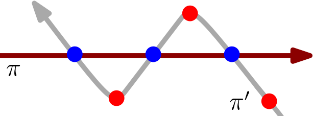
Figure 4: An example in directed graphs that demonstrates how coloring unique shortest paths with alternating colors can fail to imply low discrepancy. The nodes of path $\pi^{\prime}$ contribute discrepancy $\pm 3$ to path $\pi$; this should be contrasted with what we observe in Figure 1.

Appendix A Technical Preliminaries

Known Results in Discrepancy Theory

The first result that we discuss is the one that gives an upper bound on discrepancy of a set system in terms of primal shatter function.

Definition 5 (Primal Shatter Function).

Let $(X,\mathcal{R})$ be a set system, i.e., $X$ is a ground state and $S=\{S_{1},S_{2},\cdots,S_{\ell}\}$ with $S_{i}\subseteq X$ for all $1\leq i\leq\ell$. Let $s$ be a positive integer. The primal shatter function, denoted as $\pi_{\mathcal{R}}(s)$, is defined as $\max_{A:\,|A|=s}\left|\{A\cap S\mid S\in\mathcal{R}\}\right|$.

The following is a well known result in discrepancy theory.

Proposition A.1 (Theorem 1.8 in [Cha00]).

Given a set system $(X,\mathcal{R})$, the discrepancy of a range space $\mathcal{R}$ whose primal shatter function is bounded by $\pi_{\mathcal{R}}(s)=cs^{d}$, for some constant $c>0$, $d>1$, is

$$O(n)^{1/2-1/(2d)}(\log n)^{1+1/(2d)},$$

where $n$ is the size of the ground state, and $O(\cdot)$ hides the dependency on $c$ and $d$.

For the lower bound on hereditrary discrepancy, one tool that we use is the trace bound [CL00].

Lemma A.2 (Trace Bound [CL00]).

If $A$ is an $m$ by $n$ incidence matrix and $M=A^{T}A$, then

$$\operatorname{herdisc}(A)\geq\frac{1}{4}c^{n\operatorname{tr}(M^{2})/(\operatorname{tr}(M))^{2}}\sqrt{\frac{\operatorname{tr}(M)}{n}},$$

where $0<c<1$ is a constant.

We give various interpretation of $\operatorname{tr}(M)$ and $\operatorname{tr}(M^{2})$ in Lemma A.2 that would be useful later on. Algebraically, $\operatorname{tr}(M)$ is the sum of its eigenvalue while $\operatorname{tr}(M^{2})$ is the sum of square of the eigenvalues. Combinatorially, $\operatorname{tr}(M)$ is the number of ones in $A$ and $\operatorname{tr}(M^{2})$ is the number of rectangles of all ones in $A$. Geometrically, $\operatorname{tr}(M)$ is the count of point/region incidences and $\operatorname{tr}(M^{2})$ is number of pairs of points in all the pairwise intersections of regions. Finally, if $A$ is the incidence matrix for shortest path, $\operatorname{tr}(M^{2})$ is the number of length $4$ cycles in the underlying graph. Based on the algebraic interpretation, it means that the trace bound is non-trivial whenever all the eigenvalues of $A$ are fairly uniform. This can be seen by noticing that, if $\{\lambda_{1},\cdots,\lambda_{n}\}$ are eigenvalues of $A$, then

$${\operatorname{tr}(M)^{2}\over\operatorname{tr}(M)}=n\cos^{2}(\theta),$$

where $\theta$ is the angle between the vector $(\lambda_{1},\cdots,\lambda_{n})$ and the all one-vector.

Concentration Inequalities

We use the following standard variants of the Chernoff-Hoeffding bound in our paper.

Proposition A.3 (Chernoff bound).

Let $X_{1},\ldots,X_{n}$ be $n$ independent random variables with support on $\{0,1\}$. Define $X:=\sum_{i=1}^{n}X_{i}$. Then, for every $\delta>0$, there is

$$\Pr\left(X\geq(1+\delta)\cdot\mathbb{E}\left[X\right]\right)\leq\exp\left(-\frac{\delta^{2}}{\delta+2}\cdot\mathbb{E}\left[X\right]\right).$$

In particular, when $\delta\in(0,1]$, there is

$$\Pr\left(\left|X-\mathbb{E}\left[X\right]\right|>\delta\cdot\mathbb{E}\left[X\right]\right)\leq 2\cdot\exp\left(-\frac{\delta^{2}\mathbb{E}\left[X\right]}{3}\right).$$

Proposition A.4 (Additive Chernoff bound).

Let $X_{1},\ldots,X_{n}$ be $n$ independent random variables with support in $[0,1]$. Define $X:=\sum_{i=1}^{n}X_{i}$. Then, for every $t>0$,

$$\Pr\left(\left|X-\mathbb{E}\left[X\right]\right|>t\right)\leq 2\cdot\exp\left(-\frac{2t^{2}}{n}\right).$$

Appendix B Discrepancy Bounds for Paths Without Consistency

In a graph when we consider simple paths without the consistency requirement, there is a strong lower bound on both vertex and edge discrepancy. In particular, we have the following theorem.

Theorem 9.

There is a planar graph $G=(V,E)$ such that the following is true for any coloring $f:V\mapsto\{-1,1\}$ of vertices $V$:

1. There is a family $\Pi$ of simple paths with $|\Pi|=O(\exp(n))$ and vertex discrepancy of $\Omega(n)$.

2. There is a family $\Pi$ of simple paths with $|\Pi|=O(n)$ and vertex discrepancy of $\Omega(\sqrt{n})$.

The same claim holds true for edge discrepancy as well.

Proof.

The first claim follows from Proposition 1.6 in [BCJP20], which says that the edge discrepancy of paths on a $k\times\ell$ grid graph is at least $\Omega(k\ell)$. To prove vertex discrepancy, we make two additional remarks about this construction. First, for our purpose it is sufficient to consider only an $n\times 2$ grid graph $G$. The set of paths in the construction of [BCJP20] consist of all paths that start from the top left corner and bottom left corner going to the right and possibly taking a subset of the vertical edges in the grid graph. The number of paths is $O(2^{n})$. Second, for vertex discrepancy, we define a companion graph $G^{\prime}$. Specifically, for each grid edge $e$ in $G$, we place a vertex $v$ of $G^{\prime}$ on $e$. We connect two vertices in $G^{\prime}$ if and only if the corresponding edges in $G$ share a common vertex. The graph $G^{\prime}$ is still planar. In additional, a path $P$ in $G$ maps to a corresponding path $P^{\prime}$ in $G^{\prime}$ where vertices on $P^{\prime}$ follow the same order of the corresponding edges on $P$. See Figure 5 for an example. Therefore the edge discrepancy in $G$ and the vertex discrepancy of $G^{\prime}$ are the same.

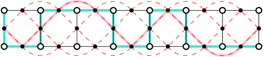
Figure 5: A $n\times 2$ grid graph (with vertices shown in hollow and edges in black) $G$ with one path (in blue) starting from the top left corner go the right. The solid vertices and edges in dashed red define the companion graph $G^{\prime}$. The corresponding path in $G^{\prime}$ is shown in pink.

For the second claim, we take an $n\times n$ Hadamard matrix $H$ with $n$ as power of $2$. The elements in $H$ are $+1$ or $-1$. Each row has $n/2$ elements of $+1$ and $n/2$ elements of $-1$ and the rows are pairwise orthogonal. It is known [Cha00] that the matrix $A=\{a_{ij}\}=\frac{1}{2}(H+J)$ with $J$ as an $n\times n$ matrix of all $1$ has discrepancy at least $\Omega(\sqrt{n})$.

Now we try to embed the matrix $A$ by paths on a $n\times 2$ grid graph $G$. Denote by $e_{j}$ as the $j$th vertical edge in $G$, $1\leq j\leq n$. For the $i$th row of $A$, we define set $X_{i}=\{e_{j}:a_{ij}=1\}$. We then define two paths $P(X_{i})$, $P^{\prime}(X_{i})$ on $G$.

• Path $P(X_{i})$ starts from the top left corner of $G$ going to the right and the vertical edges $P(X_{i})$ visits are precisely $X_{i}$.

• Path $P^{\prime}(X_{i})$ starts from the bottom left corner of $G$ going to the right and, similar to $P(X_{i})$, the vertical edges $P(X_{i})$ visits are precisely $X_{i}$.

Note that $P(X_{i})$ and $P^{\prime}(X_{i})$ each contains edges $X_{i}$ (see Figure 6 for an illustration). Also $P(X_{i})$ and $P^{\prime}(X_{i})$ do not share any horizontal edges, and collectively cover all horizontal edges in $G$. In addition, we define two paths $P$ and $P^{\prime}$ with $P$ starting from the top left corner and visiting all the top horizontal edges and $P^{\prime}$ starting from the bottom left corner and visiting all bottom horizontal edges. We have $2n+2$ paths in total – each row $i$ of the Hadamard matrix contributes $2$ paths, and we additionally use $P$ and $P^{\prime}$.

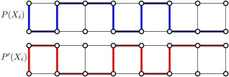
Figure 6: A $n\times 2$ grid graph $G$ with two paths $P(X_{i})$ and $P^{\prime}(X_{i})$. The $i$th row of matrix $A$, i.e., $A_{i}=(\frac{1}{2}(H+J))_{i}$, corresponds to $X_{i}=(1,1,0,1,1,1,0,0)$.

For any $\{\pm 1\}$ coloring $f$ on edges in the grid graph $G$, define $D$ as the maximum absolute value of the sum of the colors of edges of each path, among all the $2n+2$ paths. We now argue that $D=\Omega(\sqrt{n})$.

First we define an $n$-dimensional vector $\chi\in\{+1,-1\}^{n}$ with $\chi_{j}=f(e_{j})$, i.e., the color of the $j$th vertical edge in $G$. Since the discrepancy of matrix $A$ is $\Omega(\sqrt{n})$, there must be one row vector $a_{i}$ in $A$ such that $a_{i}\cdot\chi\geq c\sqrt{n}$ for some constant $c$. In other words, the sum of the colors of the edges in $X_{i}$ is $x=\sum_{e_{j}\in X_{i}}f(e_{j})$ with $|x|\geq c\sqrt{n}$. Without loss of generality, we assume $x>0$, which in turn implies $x\geq c\sqrt{n}$.

Now we define

$$z_{1}:=\sum_{e\in P(X_{i})\setminus X_{i}}f(e)\quad\text{ and}\quad z_{2}:=\sum_{e\in P^{\prime}(X_{i})\setminus X_{i}}f(e).$$

If $\max\{z_{1},z_{2}\}\geq 0$, then we are done as the total sum of colors of either $P(X)$ or $P^{\prime}(X)$ is at least $x\geq c\sqrt{n}$. Otherwise, suppose we have $z_{1}<0$ and $z_{2}<0$. We now have from path $P(X_{i})$, $D\geq x+z_{1}$, and from path $P^{\prime}(X_{i})$, $D\geq x+z_{2}$. Further, consider paths $P$ and $P^{\prime}$, the total sum of colors of all the horizontal edges is $z_{1}+z_{2}$. Since both $z_{1}$ and $z_{2}$ are negative, there should be

$$2D\geq\sum_{e\in P}f(e)+\sum_{e\in P^{\prime}}f(e)=-z_{1}-z_{2}.$$

Summing up all three inequalities, we have $4D\geq 2x$. Thus $D\geq x/2\geq c\sqrt{n}/2$. This finishes the proof for edge discrepancy, and the vertex discrepancy bound can be obtained using the same trick as in the proof of claim 1. ∎

The above theorem provides lower bounds for discrepancy. Since hereditary discrepancy is at least as high as discrepancy, the lower bounds hold for hereditary discrepancy as well.

We also want to remark that the paths used in the above theorem are $2$-approximate shortest paths. The shortest path from top left corner to the top right corner of the $n\times 2$ grid is of length $n-1$ while all paths used are of length at most $2n-2$. The shortest path from top left corner to bottom right corner is of length $n$ and all paths used in the construction are of length at most $2n-1$. Therefore when we relax from shortest paths to $2$-approximate shortest paths the discrepancy bounds substantially go up. If we allow weights on the edges we can make these paths to be $1+\varepsilon$-approximate shortest paths for any $\varepsilon>0$.

Grid graphs are a special family of planar graphs. Actually for grid graphs we can say a bit more on discrepancy of shortest paths. If we take shortest paths on an unweighted grid graph (without even requiring consistency property and there could be exponentially many shortest path between two vertices), the discrepancy is $O(1)$. Specifically, for vertex discrepancy on a $k\times\ell$ grid graph of left bottom corner at the origin and the top right corner at coordinate $(k-1,\ell-1)$, if we give a color of $+1$ to all vertices of coordinate $(x,y)$ with even $x+y$ and a color of $-1$ to all other vertices, any shortest path visits a sequence of vertices with sum of coordinates alternating between even and odd values and thus has a total color of $O(1)$. For edge discrepancy, for all horizontal edges we give color $+1$ ($-1$) if the left endpoint is at an even (odd) $x$-coordinate and the right endpoint is at an odd (even) $x$-coordinate. We do the same for vertical edges. Again any shortest path has a ‘staircase’ shape and a total coloring of $O(1)$.

Appendix C Relation Between Discrepancy and Hereditary Discrepancy in General Graphs

In Theorem 5, we showed a construction of a path weighted graph $G$ whose system of unique shortest paths $\Pi$ satisfies $\operatorname{herdisc}_{v}(\Pi)\geq\Omega(n^{1/4})$. Here, we will observe that this result extends to discrepancy:

Theorem 10.

There are examples of $n$-node undirected weighted graphs $G$ with a unique shortest path between each pair of nodes in which this system of shortest paths $\Pi$ has

$$\textnormal{disc}_{v}(\Pi)\geq\Omega(n^{1/4}).$$

Proof.

Let $G$ be the graph from Theorem 5, and let $\Pi$ be its system of unique shortest paths. By definition of hereditary discrepancy, there exists an induced path subsystem $\Pi^{\prime}\subseteq\Pi$ with

$$\operatorname{disc}_{v}(\Pi^{\prime})\geq\Omega(n^{1/4}).$$

Recall that, by induced subsystem, we mean that we may view the paths of $\Pi$ as abstract sequences of nodes, and then $\Pi^{\prime}$ is obtained from $\Pi$ by deleting zero or more nodes and deleting all occurrences of those nodes from the middle of paths. Thus the paths in $\Pi^{\prime}$ are not still paths in $\Pi$, but they are paths in a different graph $G^{\prime}$ on $n^{\prime}\leq n$ nodes. It thus suffices to argue that all paths in $\Pi^{\prime}$ are

It thus suffices to argue that there is a graph $G^{\prime}$ on $n^{\prime}\leq n$ nodes in which all paths in $\Pi^{\prime}$ are unique shortest paths. Indeed, this is well known, and is shown e.g. in [Bod19] (c.f. Lemma 2.4.4 and 2.4.11). To sketch the proof: suppose that a node $v$ is deleted from the initial system $\Pi$. Consider each path $\pi\in\Pi$ that contains $v$ as an internal node, i.e., it has the form

$$\pi=(\dots,u,v,x,\dots).$$

When $v$ is removed, the path now contains the nodes $u,x$ consecutively, and so we must add $(u,x)$ as a new edge to $G^{\prime}$ so that $\pi$ is a path in $G^{\prime}$. We judiciously set the edge weight to be $w(u,x):=w(u,v)+w(v,x)$. The weighted length of the path $\pi$ does not change, and yet the distances of $G^{\prime}$ majorize those of $G$, which implies that $\pi$ is still a unique shortest path in $G^{\prime}$. Inducting this analysis over each deleted vertex leads to the desired claim. ∎

Appendix D Application in Matrix Analysis

Hereditary discrepancy is intrinsically related to factorization norm, which has found applications in many ares of computer science, including but not limited to quantum channel capacity, communication complexity, etc. For any complex matrix $A\in\mathbb{C}^{m\times n}$, its factorization norm, denoted by $\gamma_{2}(A)$, is defined as the following optimization problem:

$$\gamma_{2}(A)=\min\left\{\|L\|_{2\to\infty}\|R\|_{1\to 2}:A=LR\right\}.$$ (1)

Here, for $p,q\in\mathbb{N}_{\geq 0}$,

$$\|{A}\|_{p\to q}=\max\frac{\|Ax\|_{q}}{\|x\|_{p}}.$$

One can write eq 1 in a form of a semi-definite program (see Lee et al. [LSŠ08]) and also show that the Slater point exists. In particular, the primal and dual program coincides. An interesting question in matrix analysis is to estimate the factorization norm of different class of matrices. In a series of work, various authors have computed tight bounds on the factorization norm of certain class of matrices:

• If $A$ is a unitary matrix, then $\gamma_{2}(A)=1$ [Sch11].

• If $A\in\mathbb{R}^{n\times n}$ is a positive semidefinite matrix with entries $A_{ij}$ [Sch11], then

  $$\gamma_{2}(A)=\max_{1\leq i\leq n}A_{ii}.$$

• Mathias [Mat93] $A$ satisfies the property that $\sqrt{A^{\top}A}\bullet\mathbb{I}=\sqrt{AA^{\top}}\bullet\mathbb{I}={\operatorname{tr}(A)\over n}\mathbb{I}$, then

  $$\gamma_{2}(A)={\mathsf{Tr}(A^{\top}A)\over n}.$$

  In particular, if $A\in\{0,1\}^{n}$ is a lower-triangular one $1$ matrix, then $\gamma_{2}(A)=\Theta(\log n)$ [FHU23, HUU23, KP70].

• If $A\in\mathbb{R}^{n\times n}$ is a lower-triangular Toeplitz matrix with entries decreasing either polynomially or exponentially, then $\gamma_{2}(A)=\Theta(1)$ [HUU24].

Our tight bound on hereditary discrepancy for consistent path on graphs allows us to give tight bound on the factorization norm for the corresponding incidence matrix. In particular, we use the following result:

Lemma D.1 (Matoušek et al. [MNT20]).

For any real $m\times n$ matrix $A\in\mathbb{R}^{m\times n}$, there exists absolute constants $0<c<C$ such that

$$c\frac{\gamma_{2}(A)}{\sqrt{\log(m)}}\leq\operatorname{herdisc}(A)\leq C\gamma_{2}(A)\log(m).$$

Combining Lemma D.1 with our results, we have the following corollary:

Corollary D.2.

Let $A_{G}$ be the incident matrix for unique shortest path system on an $n$ vertices graph $G$. Then if $G$ is bipartite, planar, or any general graph, then $\gamma_{2}(A_{G})=\widetilde{\Theta}(n^{1/4})$.

Appendix E Proof of 2.3

For completeness we recall 2.3 as follows, and then present the proof.

Observation E.1.

Denote by $\operatorname{disc}(n)$ (and $\operatorname{herdisc}(n)$) the maximum discrepancy (minimum hereditary discrepancy, respectively) of a consistent path system of a (undirected or directed) graph of $n$ vertices. We have that

1. Let $g(x)$ be a non-decreasing function of $x$. If $\textnormal{herdisc}_{v}(n)\geq g(n)$, then $\textnormal{herdisc}_{e}(n)\geq g(n/2)$.

2. Let $f(x)$ be a non-decreasing function of $x$. If $\textnormal{disc}_{v}(n)\leq f(n)$, then $\textnormal{disc}_{e}(m)\leq f(m)$.

Proof.

We prove Item 1 by showing that if graph $G=(V,E,w)$ with the consistent path matrix $A^{(v)}$ has hereditary discrepancy at least $g(n)$, we can obtain another graph $G^{\prime}=(V^{\prime},E^{\prime},w^{\prime})$ and matrix $A^{(e)}$ as the (consistent path) edge incidence matrix with hereditary discrepancy at least $g(n/2)$. The construction is as follows.

1. We first split each vertex $v\in V$ in $G$ to two vertices $(v_{in},v_{out})$ to obtain $V^{\prime}$.

2. For every $v\in V$, add a single edge $(v_{in},v_{out})$ to $E^{\prime}$.

3. For any $v\in V$ and each edge $(u,v)\in E$ (with the fixed $v$), add edges $(u_{out},v_{in})$ and $(u_{in},v_{out})$ to $E^{\prime}$.

The path incident matrix $A^{(e)}$ is defined as follows: for each path as a row $a$ of $A^{(v)}$, construct a new path in $G^{\prime}$ by following the order of $u_{out}\rightarrow v_{in}\rightarrow v_{out}\rightarrow w_{in}$ for a $u\rightarrow v\rightarrow w$ sequence. For each row in $A^{(v)}$, we mark the used edges as $1$ in $A^{(e)}$ with the path constructed by the above process. Note that the new path system defined by $A^{(e)}$ remains consistent: for any intersection between the two paths $P_{1}\cap P_{2}=(u_{1},u_{2},\cdots,u_{\ell})$, the intersection remains a single path of $(u_{1,in},u_{1,out},\cdots,u_{\ell,in},u_{\ell,out})$ in $A^{(e)}$.

Let $Y$ be the columns that induces the $g(n)$ discrepancy on $G$, i.e.,

$$\min_{x\in\{-1,+1\}^{\left|Y\right|}}\|A^{(v)}_{Y}x\|_{\infty}=g(n).$$

Now, observe that, for each row in $A^{(e)}$, an edge $(v_{in},v_{out})$ is marked as $1$ if and only if $v$ is marked as $1$ in $A^{(v)}$. Therefore, we can take the new set $Y^{\prime}$ as the edges corresponding to $Y$, and there is

$$\min_{x\in\{-1,+1\}^{\left|Y^{\prime}\right|}}\|A^{(e)}_{Y^{\prime}}x\|_{\infty}=\min_{x\in\{-1,+1\}^{\left|Y\right|}}\|A^{(v)}_{Y}x\|_{\infty}=g(n).$$

Finally, since graph $G^{\prime}$ has $n^{\prime}=2n$ vertices, we have the hereditary discrepancy to be at least $g(n^{\prime}/2)$, as desired.

For Item 2, we show that the hereditary edge discrepancy of $G$ is at most $f(m)$, which implies the discrepancy upper bound. For a graph with $n$ vertices, $m$ edges, and a path incident matrix $A^{(e)}$, suppose $Y$ is the set of columns (edges) that attain the hereditary discrepancy. We can add a vertex $v_{e}$ for each $e\in Y$ and construct a new path incident matrix $A^{(v)}$, which is a matrix with $\left|Y\right|$ rows. Concretely, for each row of $A^{(v)}$, we simply let vertices $v_{e}\in Y$ be $1$ if the corresponding edge is used in $A^{(e)}$. By the consistency of $A^{(e)}$, the new path incident matrix also characterizes a consistent path system (we can think of the underlying graph as the complete graph on vertex set of $Y$). Note that since there are at most $m$ vertices in $A^{(e)}$, we can get $f(m)$ discrepancy for the path system characterized by $A^{(e)}$. This implies a $f(m)$ hereditary edge discrepancy on the original path system, which in turn implies the desired discrepancy upper bound.

Finally, note that the argument remains valid when the graph is directed, which means the results hold for both undirected and directed graphs. ∎

Appendix F Differentially Private All Sets Range Queries

Here we introduce the DP-ASRQ problem and show its connection to the DP-APSD problem.

Given an undirected graph $G$, the problem of All Sets Range Queries (ASRQ) considers each edge associated with a certain attribute, and the range is the set of edges along a shortest path. Two type of queries are considered here: the bottleneck query returns the largest/smallest attribute in a range; while the counting query returns the summation of all attributes.

At a schematic level, the ASRQ problem with counting queries is very similar to the APSD problem: the graph topology is public and the edge attributes are considered private. Only that the shortest path structure is dictated by the edge weights to be protected in the APSD problem, however, irrelevant to the edge attributes in the ASRQ problem. This subtle difference has consequential caveat in the algorithm design: the graph topology can be used, for example, to construct an exact hopset first then apply perturbations to the edge attributes in the ASRQ problem; nevertheless, approach of this kind violates protecting the sensitive information in the APSD problem, since adversarial inference can be made on edge weights when the graph topology information is used. This observation also notes that the APSD problem is strictly harder than the ASRQ problem: recall that the best additive error upper bound of the APSD problem is still $\widetilde{O}(n^{1/2})$, while the other has $\widetilde{O}(n^{1/4})$ [DGUW23]. Therefore, plugging in our new hereditary lower bound essentially closes the gap for the ASRQ problem.

Corollary F.1 (Formal version of Theorem 4).

Given an $n$-node undirected graph, for any $\beta\in(0,1)$ and any $\varepsilon,\delta>0$, no $(\varepsilon,\delta)$-DP algorithm for ASRQ has additive error of $o(n^{1/4})$ with probability $1-\beta$.

Definition 6 (Neighboring weights [Sea16]).

For a graph $G=(V,E)$, let $w,w^{\prime}:E\rightarrow\mathbb{R}^{\geq 0}$ be two weight functions that map any $e\in E$ to a non-negative real number, we say $w,w^{\prime}$ are neighboring, denoted as $w\sim w^{\prime}$ if $\sum_{e\in E}|w(e)-w^{\prime}(e)|\leq 1.$

Definition 7 (Differentially Private Range Queries).

Let $(\mathcal{R}=(X,\mathcal{S}),f)$ be a system of range queries and $w,w^{\prime}:X\rightarrow\mathbb{R}^{\geq 0}$ be neighboring attribute functions. Furthermore, let $\mathcal{A}$ be an algorithm that takes $(\mathcal{R},f,w)$ as input. Then $\mathcal{A}$ is $(\varepsilon,\delta)$-differentially private on $G$ if, for all pairs of neighboring attribute functions $w,w^{\prime}$ and all sets of possible outputs $\mathcal{C}$, we have $\Pr[\mathcal{A}(\mathcal{R},f,w)\in\mathcal{C}]\leq e^{\varepsilon}\cdot\Pr[\mathcal{A}(\mathcal{R},f,w^{\prime})\in\mathcal{C}]+\delta.$ If $\delta=0$, we say $\mathcal{A}$ is $\varepsilon$-differentially private on $G$.

To complete this section, we give the formal definition of the ASRQ problem above. The definition of neighboring attributes follows Definition 6. The lower bound proof of Corollary F.1 simply imitates the APSD problem, because the reduction from the linear query problem still holds despite the difference between two problems. The proof is omitted to avoid redundancy.

References

- [ABC04] J Ralph Alexander, József Beck, and William WL Chen. Geometric discrepancy theory and uniform distribution. Handbook of discrete and computational geometry, page 279, 2004.
- [AFGW10] Ittai Abraham, Amos Fiat, Andrew V Goldberg, and Renato F Werneck. Highway dimension, shortest paths, and provably efficient algorithms. In Proceedings of the twenty-first annual ACM-SIAM symposium on Discrete Algorithms, pages 782–793. SIAM, 2010.
- [AW20] Saeed Akhoondian Amiri and Julian Wargalla. Disjoint shortest paths with congestion on DAGs. arXiv preprint arXiv:2008.08368, 2020.
- [AW23] Shyan Akmal and Nicole Wein. A local-to-global theorem for congested shortest paths. In 31st Annual European Symposium on Algorithms (ESA 2023), pages 8:1–8:17, 2023.
- [Bal22] Lorenzo Balzotti. Non-crossing shortest paths are covered with exactly four forests. arXiv preprint arXiv:2210.13036, 2022.
- [BCJP20] József Balogh, Béla Csaba, Yifan Jing, and András Pluhár. On the discrepancies of graphs. Electronic Journal of Combinatorics, 27(2), 2020.
- [BDF+22] Johannes Blum, Yann Disser, Andreas Emil Feldmann, Siddharth Gupta, and Anna Zych-Pawlewicz. On sparse hitting sets: From fair vertex cover to highway dimension. arXiv preprint arXiv:2208.14132, 2022.
- [BDG+16] Hannah Bast, Daniel Delling, Andrew Goldberg, Matthias Müller-Hannemann, Thomas Pajor, Peter Sanders, Dorothea Wagner, and Renato F Werneck. Route planning in transportation networks. Algorithm engineering: Selected results and surveys, pages 19–80, 2016.
- [BH23] Greg Bodwin and Gary Hoppenworth. Folklore sampling is optimal for exact hopsets: Confirming the barrier. In Proceedings of the 64th IEEE Symposium on Foundations of Computer Science (FOCS) 2023, 2023.
- [Bod19] Greg Bodwin. On the structure of unique shortest paths in graphs. In Proceedings of the Thirtieth Annual ACM-SIAM Symposium on Discrete Algorithms, pages 2071–2089. SIAM, 2019.
- [CCL+23a] Hsien-Chih Chang, Jonathan Conroy, Hung Le, Lazar Milenkovic, and Shay Solomon. Covering planar metrics (and beyond): O(1) trees suffice. arXiv preprint arXiv:2306.06215, 2023.
- [CCL23b] Maria Chudnovsky, Daniel Cizma, and Nati Linial. The structure of metrizable graphs. arXiv preprint arXiv:2311.09364, 2023.
- [CE06] Don Coppersmith and Michael Elkin. Sparse sourcewise and pairwise distance preservers. SIAM Journal on Discrete Mathematics, 20(2):463–501, 2006.
- [CGK+23] Justin Y. Chen, Badih Ghazi, Ravi Kumar, Pasin Manurangsi, Shyam Narayanan, Jelani Nelson, and Yinzhan Xu. Differentially private all-pairs shortest path distances: Improved algorithms and lower bounds. In SODA, 2023.
- [CGMW18] Hsien-Chih Chang, Pawel Gawrychowski, Shay Mozes, and Oren Weimann. Near-optimal distance emulator for planar graphs. In 26th Annual European Symposium on Algorithms (ESA 2018), pages 16:1–16:17, 2018.
- [CGW89] Fan R. K. Chung, Ronald L. Graham, and Richard M. Wilson. Quasi-random graphs. Combinatorica, 9:345–362, 1989.
- [Cha00] Bernard Chazelle. The Discrepancy Method: Randomness and Complexity. Cambridge University Press, 2000.
- [CKT22] Hsien-Chih Chang, Robert Krauthgamer, and Zihan Tan. Near-linear -emulators for planar graphs. arXiv preprint arXiv:2206.10681, 2022.
- [CL00] Bernard Chazelle and Alexey Lvov. A trace bound for the hereditary discrepancy. In Proceedings of the sixteenth annual symposium on Computational geometry, SCG ’00, pages 64–69, New York, NY, USA, May 2000. Association for Computing Machinery.
- [CL22] Daniel Cizma and Nati Linial. Geodesic geometry on graphs. Discrete & Computational Geometry, 68(1):298–347, 2022.
- [CL23] Daniel Cizma and Nati Linial. Irreducible nonmetrizable path systems in graphs. Journal of Graph Theory, 102(1):5–14, 2023.
- [CLRS22] Thomas H Cormen, Charles E Leiserson, Ronald L Rivest, and Clifford Stein. Introduction to algorithms. MIT press, 2022.
- [DGUW23] Chengyuan Deng, Jie Gao, Jalaj Upadhyay, and Chen Wang. Differentially private range query on shortest paths. In Algorithms and Data Structures Symposium, pages 340–370. Springer, 2023.
- [DMNS06] Cynthia Dwork, Frank McSherry, Kobbi Nissim, and Adam Smith. Calibrating noise to sensitivity in private data analysis. In Theory of Cryptography: Third Theory of Cryptography Conference, TCC 2006, New York, NY, USA, March 4-7, 2006. Proceedings 3, pages 265–284. Springer, 2006.
- [DR14] Cynthia Dwork and Aaron Roth. The algorithmic foundations of differential privacy. Foundations and Trends® in Theoretical Computer Science, 9(3–4):211–407, 2014.
- [FHU23] Hendrik Fichtenberger, Monika Henzinger, and Jalaj Upadhyay. Constant matters: Fine-grained error bound on differentially private continual observation. In International Conference on Machine Learning, pages 10072–10092. PMLR, 2023.
- [FLL22] Chenglin Fan, Ping Li, and Xiaoyun Li. Breaking the linear error barrier in differentially private graph distance release. arXiv preprint arXiv:2204.14247, 2022.
- [HKRS97] Monika R Henzinger, Philip Klein, Satish Rao, and Sairam Subramanian. Faster shortest-path algorithms for planar graphs. Journal of Computer and System Sciences, 55(1):3–23, 1997.
- [HP11] Sariel Har-Peled. A simple proof of the existence of a planar separator. arXiv preprint arXiv:1105.0103, 2011.
- [HUU23] Monika Henzinger, Jalaj Upadhyay, and Sarvagya Upadhyay. Almost tight error bounds on differentially private continual counting. In Proceedings of the 2023 Annual ACM-SIAM Symposium on Discrete Algorithms (SODA), pages 5003–5039. SIAM, 2023.
- [HUU24] Monika Henzinger, Jalaj Upadhyay, and Sarvagya Upadhyay. A unifying framework for differentially private sums under continual observation. In Symposium on Disrete Algorithms, 2024.
- [KP70] Stanisław Kwapień and Aleksander Pełczyński. The main triangle projection in matrix spaces and its applications. Studia Mathematica, 34(1):43–67, 1970.
- [KP22] Shimon Kogan and Merav Parter. New diameter-reducing shortcuts and directed hopsets: Breaking the barrier. In Proceedings of the 2022 Annual ACM-SIAM Symposium on Discrete Algorithms (SODA), pages 1326–1341. SIAM, 2022.
- [LSŠ08] Troy Lee, Adi Shraibman, and Robert Špalek. A direct product theorem for discrepancy. In 2008 23rd Annual IEEE Conference on Computational Complexity, pages 71–80. IEEE, 2008.
- [Mat93] Roy Mathias. The hadamard operator norm of a circulant and applications. SIAM journal on matrix analysis and applications, 14(4):1152–1167, 1993.
- [Mat99] Jiři Matoušek. Geometric Discrepancy: An Illustrated Guide. Springer Science & Business Media, May 1999.
- [MN12] Shanmugavelayutham Muthukrishnan and Aleksandar Nikolov. Optimal private halfspace counting via discrepancy. In Proceedings of the forty-fourth annual ACM symposium on Theory of computing, pages 1285–1292, 2012.
- [MNT20] Jiří Matoušek, Aleksandar Nikolov, and Kunal Talwar. Factorization norms and hereditary discrepancy. International Mathematics Research Notices, 2020(3):751–780, 2020.
- [PA11] János Pach and Pankaj K Agarwal. Combinatorial Geometry. John Wiley & Sons, October 2011.
- [Sch11] Jssai Schur. Remarks on the theory of bounded bilinear forms with infinitely many variables. 1911.
- [Sea16] Adam Sealfon. Shortest paths and distances with differential privacy. In Proceedings of the 35th ACM SIGMOD-SIGACT-SIGAI Symposium on Principles of Database Systems, pages 29–41, 2016.
- [TOG17] C D Toth, J O’Rourke, and J E Goodman. Handbook of discrete and computational geometry. 2017.