On the partial autocorrelation function for locally stationary time series: characterization, estimation and inference

Abstract

For stationary time series, it is common to use the plots of partial autocorrelation function (PACF) or PACF-based tests to explore the temporal dependence structure of such processes. To our best knowledge, such analogs for non-stationary time series have not been fully established yet. In this paper, we fill this gap for locally stationary time series with short-range dependence. First, we characterize the PACF locally in the time domain and show that the $j$th PACF, denoted as $\rho_{j}(t),$ decays with $j$ whose rate is adaptive to the temporal dependence of the time series $\{x_{i,n}\}$. Second, at time $i,$ we justify that the PACF $\rho_{j}(i/n)$ can be efficiently approximated by the best linear prediction coefficients via the Yule-Walker’s equations. This allows us to study the PACF via ordinary least squares (OLS) locally. Third, we show that the PACF is smooth in time for locally stationary time series. We use the sieve method with OLS to estimate $\rho_{j}(\cdot)$ and construct some statistics to test the PACFs and infer the structures of the time series. These tests generalize and modify those used for stationary time series in Brockwell & Davis (1987). Finally, a multiplier bootstrap algorithm is proposed for practical implementation and an $\mathtt{R}$ package $\mathtt{Sie2nts}$ is provided to implement our algorithm. Numerical simulations and real data analysis also confirm usefulness of our results.

section Introduction

The partial autocorrelation function (PACF) is one of the most popular and powerful tools for stationary time series modelling and analysis Brockwell & Davis (1987). However, in the era of big data, as increasingly longer time series are being collected, it has become more appropriate to model many of those series as locally stationary processes whose data generating mechanisms evolve smoothly over time. In this setting, the effectiveness of the classical PACF deteriorates and it is of urgent demand to establish the theories of PACF for locally stationary time series.

Even though there exists a rich body of literature on locally stationary time series analysis, see Dahlhaus (2012); Dahlhaus et al. (2019) for a review, much less has been studied related to the PACF. In Dégerine & Lambert-Lacroix (2003), the authors generalized the characterization of PACFs via some useful decomposition as introduced in Ramsey (1974) to general non-stationary processes. They also briefly discussed how to estimate the PACFs based on a generalized Levinson-Durbin algorithm when the autocovariance function is given. More recently, in Killick et al. (2020), by generalizing the partial autocorrelations of stationary processes to locally stationary time series from a wavelet spectrum perspective, the authors provided two new estimators for the local PACFs. The consistency of the wavelet-based estimator and the asymptotic distribution of the windowed estimator under Gaussian assumption have also been studied. However, the decay speed of local PACFs as a function of the lags has not been established and a direct time-domain characterization of the PACFs of locally stationary processes has not been fully investigated. Moreover, the inference for PACFs of locally stationary time series, for example significance tests and PACF-based Portmanteau tests, are still missing in the literature.

Motivated by the above challenges, in this paper, we aim to systematically study the theories of PACFs for locally stationary time series. For characterization, in contrast to Dégerine & Lambert-Lacroix (2003); Killick et al. (2020), we define PACFs for general locally stationary time series in the time domain using stationary approximations at each time point (c.f. Definition section.thm). There are several advantages in using this characterization. First, since the time series is approximately stationary locally, the lower-order PACFs can be well approximated by the best short-term linear prediction coefficients via the Yule-Walker equations; see (section.equation) and (section.equation). This connection not only allows us to study the PACF via ordinary least squares (OLS) estimation but also enables us to establish the decay properties of the PACFs which are adaptive to the temporal dependence decay of the time series; see (section.equation). Second, the smoothness of the locally stationary covariance structure can be easily translated to that of the PACFs; see (section.equation). Therefore, it suffices to estimate some smooth functions $\rho_{j}(\cdot)$ at different lags $j.$ More specifically, together with the OLS, the smooth PACFs can be estimated adaptively using the nonparametric method of sieves via flexible choices of basis functions such as the wavelets and the orthogonal polynomials Chen (2007); see Section section.subsection. Theoretically, under mild assumptions, the estimators are consistent uniformly in the time domain (c.f. Theorem section.thm). Third, based on the time-domain characterization and the OLS form of the sieve estimators, one can further conduct various tests on the PACFs. For example, one can perform a white noise Portmanteau test or significance tests on some PACFs (e.g., checking the order for an AR process) uniformly over time and lags. Both tests have not been fully studied yet under the locally stationary time series framework. We establish the asymptotic normality and conduct a power analysis for the tests (c.f. Theorems section.thm and section.thm). We also propose a multiplier bootstrap procedure for practical implementation (c.f. Algorithm 1). Numerical simulations and real data analysis are provided to illustrate the usefulness of our results and an $\mathtt{R}$ package $\mathtt{Sie2nts}$ is provided for users. Since our method covers stationary time series as a special case, we promote the use of the $\mathtt{Sie2nts}$ package instead of the default $\mathtt{pacf}$ function in $\mathtt{R}$ which only handles stationary time series.

The paper is organized as follows. In Section section, we provide the characterization of the PACFs for locally stationary time series and study their asymptotic properties. In Section section, we introduce our estimator for PACFs based on the nonparametric sieve method and inference procedures based on multiplier bootstrap. In Section section, we provide theoretical analysis for our estimation and inference procedures. Numerical simulations and real data analysis are offered in Section section. More details are provided in our online supplement Ding & Zhou (2024). Especially, technical proofs are deferred to Section A, further discussions and remarks are provided in Section B, some tuning parameter selection algorithm is listed in Section C and additional simulation results are offered in Section D.

Conventions. For a random variable $x\in\mathbb{R}$ and some constant $q\geq 1,$ we denote by $\|x\|_{q}:=(\mathbb{E}|x|^{q})^{1/q}$ its $L^{q}$ norm. We simply write $\|x\|\equiv\|x\|_{2}$ when $q=2.$ For any deterministic vector $\bm{x}=(x_{1},x_{2},\cdots,x_{p})^{*}\in\mathbb{R}^{p},$ we use $|x|=\sqrt{\sum_{i=1}^{p}x_{i}^{2}}$ for its $\ell_{2}$ (or Euclidean) norm. For any matrix $A,$ we use $\|A\|$ to stand for its operator norm. For two sequences of deterministic positive values $\{a_{n}\}$ and $\{b_{n}\}$, we write $a_{n}=\mathrm{O}(b_{n})$ if $a_{n}\leq Cb_{n}$ for some positive constant $C>0$. Moreover, we write $a_{n}=\mathrm{o}(b_{n})$ if $a_{n}\leq c_{n}b_{n}$ for some positive sequence $c_{n}\downarrow 0.$ For a sequence of random variables $\{x_{n}\}$ and positive real values $\{a_{n}\},$ we use the notation $x_{n}=\mathrm{O}_{\ell^{q}}(a_{n})$ to state that $x_{n}/a_{n}$ is bounded in $L^{q}$ norm; that is $\|x_{n}/a_{n}\|_{q}\leq C$ for some finite constant $C>0.$ If $q=1,$ we simply write $x_{n}=\mathrm{O}_{\mathbb{P}}(a_{n}).$ We use $\mathbf{I}_{c}$ for a $c\times c$ identity matrix. We use $C^{d}([0,1])$ for the function space on $[0,1]$ of continuous functions that have continuous first $d$ derivatives.

section Characterization of PACF for locally stationary time series

In this section, we provide the characterization of PACF of locally stationary time series and study its properties. Suppose that we observe $\{x_{i,n}\}_{i=1}^{n}$. For simplicity and without loss of generality, we assume the time series is centered (i.e., mean is zero). Till the end of the paper, for notional simplicity, we always write $x_{i}\equiv x_{i,n}.$ From time to time, we will emphasize the dependence on $n$ for various quantities.

In this paper, we focus on a general class of locally stationary time series following definition introduced in Ding & Zhou (2023). It covers many commonly used locally stationary time series models in the literature. See for instance Ding & Zhou (2020); Dahlhaus et al. (2019); Dahlhaus (2012); Roueff & Sanchez-Perez (2018); Kley et al. (2019); Dette et al. (2011); Dette & Wu (2020); Vogt (2012); Zhou & Wu (2009). We refer the readers to Example B.thm in our supplement for more details.

Definition section.thm (Locally stationary time series and its PACF).

A non-stationary time series $\{x_{i}\}$ is a locally stationary time series (in covariance) if there exists a function $\gamma(t,k):[0,1]\times\mathbb{N}\rightarrow\mathbb{R}$ such that

$$\operatorname{Cov}(x_{i},x_{j})=\gamma(t_{i},|i-j|)+\mathrm{O}\left(\frac{|i-j|+1}{n}\right),\ t_{i}=\frac{i}{n}.$$ (section.equation)

Moreover, we assume that $\gamma$ is Lipschitz continuous in $t$ and for any fixed $t\in[0,1],$ $\gamma(t,\cdot)$ is the autocovariance function (ACF) of some stationary process whose $j$th order PACF is denoted as $\rho_{j}(t)$. We shall also call $\rho_{j}(t)$ the $j$th order PACF at rescaled time $t$ of $\{x_{i}\}.$

Observe that Definition section.thm essentially means that the covariance structure of $\{x_{i}\}$ can be well approximated locally by that of a stationary process. Consequently, at each rescaled time $t$, the PACF of $\{x_{i}\}$ is defined by that of the approximating stationary process. Now we study the PACF introduced above. Since only one realization of the series $\{x_{i}\}$ is available, we will need to assume short-range dependence that for some $\tau>1,$

$$\max_{k,n}\left|\operatorname{Cov}(x_{k,n},x_{k+r,n})\right|=\mathrm{O}\left(|r|^{-\tau}\right)\ \text{and}\ \sup_{t}|\gamma(t,|r|)|=\mathrm{O}(|r|^{-\tau}),$$ (section.equation)

and add additional regularity conditions. These will be summarized in Assumption section.thm after some necessary notations are introduced. For the autocovariance function $\gamma(t,\cdot)$ in (section.equation), given a lag $j,$ we define a vector of functions $\bm{\phi}_{j}(t)=(\bm{\phi}_{j,1}(t),\cdots,\bm{\phi}_{j,j}(t))^{*}:[0,1]\rightarrow\mathbb{R}^{j}$ via the local Yule-Walker equation

$$\bm{\phi}_{j}(t)=\Gamma_{j}(t)^{-1}\bm{\nu}_{j}(t),$$ (section.equation)

where $\Gamma_{j}(t)\in\mathbb{R}^{j\times j}$ is a symmetric matrix whose $(k,l)$ entry is defined as $\Gamma_{j}^{(k,l)}(t):=\gamma(t,|k-l|),$ and $\bm{\nu}_{j}(t)\in\mathbb{R}^{j}$ is vector whose $k$th entry is defined as $\bm{\nu}_{j}^{(k)}(t):=\gamma(t,k).$ Consequently, we can write Brockwell & Davis (1987)

$$\rho_{j}(t)=\bm{\phi}_{j,j}(t).$$ (section.equation)

Note that for stationary time series the PACF is closely related to the best linear forecast coefficients of the process (Brockwell & Davis (1987)). The representation (section.equation) together with the smoothness of the time series covariance structure imply that we can study the PACF of locally stationary time series via local best linear forecasts and therefore a simple local regression analysis. Specifically, for all $1\leq j\leq i-1,$ denote the $j$th order best linear forecast of $x_{i}$ as $\widehat{x}_{i,j}=\sum_{k=1}^{j}\phi_{ik,j}x_{i-k},$ where $\phi_{ik,j}\equiv\phi_{ik,j,n},\ 1\leq k\leq j,$ are the best linear forecast coefficients. Define the residual as $\epsilon_{i,j}\equiv\epsilon_{i,j,n}:=x_{i}-\widehat{x}_{i,j}.$ We now write

$$x_{i}=\sum_{k=1}^{j}\phi_{ik,j}x_{i-k}+\epsilon_{i,j}.$$ (section.equation)

Using (section.equation), we introduce the following notations

$$\rho_{i,j}=\phi_{ij,j},\ 1\leq j\leq i-1.$$ (section.equation)

The following theorem studies the uniform decay property of the PACF and builds the connection between the PACF defined in Definition section.thm and $\rho_{i,j}$ in (section.equation) for the locally stationary time series.

Theorem section.thm.

For the locally stationary time series $\{x_{i}\}$ satisfying Definition section.thm, suppose Assumption section.thm holds. Then we have the followings holds.

1. For $\tau$ in (section.equation), we have that for $\rho_{j}(t)$ in Definition section.thm and $\rho_{i,j}$ in (section.equation)

   $$\sup_{i>j}|\rho_{i,j}|=\mathrm{O}\left(\left(\frac{\log j+1}{j}\right)^{\tau-1}\right)\ \text{and}\ \sup_{t}|\rho_{j}(t)|=\mathrm{O}\left(\left(\frac{\log j+1}{j}\right)^{\tau-1}\right).$$ (section.equation)

2. $\rho_{j}(t)\in C^{d}([0,1]),$ for some integer $d>0$ defined in (section.equation) and

   $$\sup_{i>j}\left|\rho_{j}\left(\frac{i}{n}\right)-\rho_{i,j}\right|=\mathrm{O}\left(\frac{j^{2}}{n}\right).$$ (section.equation)

Remark section.thm.

Several remarks on Theorem section.thm are in order. First, (section.equation) implies that, uniformly over time, the PACF decays polynomially fast to 0 as a function of the lag with the speed adaptive to that of the autocovariance. If $\tau$ is sufficiently large, this implies that practically we only need to consider the first few lags of the PACF. In practice, people are usually concerned with the cutoff that $\sup_{t}|\rho_{j}(t)|\gg n^{-1/2}.$ In this sense, we conclude from (section.equation) that we only need to focus on the lags for $j=\mathrm{O}\left(n^{\frac{1}{2(\tau-1)}}\right).$ Second, (section.equation) demonstrates that under Definition section.thm and Assumption section.thm, the PACFs can be well approximated by $\rho_{i,j}$ if $j$ is not too large. Observe that $\rho_{i,j}$ is defined by local best linear forecasts and therefore is closely related to OLS. Therefore, (section.equation) lays the theoretical foundation for the estimation and inference procedures in Section section.

section Estimation and inference procedures

In this section, we provide the procedures of the estimation and inference of the PACFs of locally stationary time series. The theoretical justifications will be provided in Section section. As mentioned in Remark section.thm, in what follows, we shall only consider lag $j\leq j_{*}$ with

$$j_{*}\asymp n^{\frac{1}{2(\tau-1)}}.$$ (section.equation)

section.subsection Sieve nonparametric estimation

In this section, we estimate the PACFs $\rho_{j}(\cdot).$ As proved in Theorem section.thm, since $\rho_{j}(t)\in C^{d}([0,1]),$ it is natural for us to approximate it via a finite diverging term basis expansion using the method of sieves as in Chen (2007); Ding & Zhou (2020, 2023). Recall $\rho_{j}(t)$ is defined via $\bm{\phi}_{j}(t)$ in (section.equation). Now we will work with $\bm{\phi}_{j}(t).$

According to (Chen, 2007, Section 2.3), we have that for some pre-chosen orthonormal basis functions on $[0,1]$, denoted as $\{\alpha_{k}(t)\}$

$$\bm{\phi}_{j,l}(t):=\sum_{k=1}^{c}a_{jk,l}\alpha_{k}(t)+\mathrm{O}(c^{-d}),\ 1\leq l\leq j,$$ (section.equation)

where $c$ is the number of basis functions. Here $\{a_{jk,l}\}$ are the coefficients to be estimated. In fact, using (Ding & Zhou, 2023, Theorem 2.11) and a discussion similar to (3.8) therein, we have by (section.equation) that

$$x_{i}=\sum_{l=1}^{j}\sum_{k=1}^{c}a_{jk,l}z_{kl}+\epsilon_{i,j}+\mathrm{O}_{\ell^{2}}\left(j^{2}/n+jc^{-d}\right),\ i>j,$$ (section.equation)

where $\epsilon_{i,j}$ is defined in (section.equation) and $z_{kl}(i/n)=\alpha_{k}(i/n)x_{i-l}$. Observe that a key component in (section.equation) is the approximation of $\rho_{j}(\cdot)$ by local best linear forecast coefficients as in (section.equation).

Using (section.equation), we can estimate all the coefficients $a_{jk,l}$’s using one OLS regression. In particular, we stack $a_{jk,l},1\leq l\leq j,1\leq k\leq c$ as a vector $\bm{\beta}_{j}\in\mathbb{R}^{jc},$ then the OLS estimator for $\bm{\beta}_{j}$ can be written as $\widehat{\bm{\beta}}_{j}:=(Y_{j}^{*}Y_{j})^{-1}Y_{j}^{*}\bm{x}_{j},$ where $Y_{j}^{*}\in\mathbb{R}^{jc\times(n-j)}$ is the design matrix of (section.equation) and $\bm{x}_{j}=(x_{j+1},\cdots,x_{n})^{*}\in\mathbb{R}^{n-j}.$

After estimating the $a_{jk,l}$’s, $\rho_{j}(t)\equiv\bm{\phi}_{j,j}(t)$ is estimated using (section.equation) as

$$\widehat{\rho}_{j}(t)=\widehat{\bm{\beta}}_{j}^{*}\mathbb{B}_{j,j}(t),$$ (section.equation)

where $\mathbb{B}_{j,l}(t)\in\mathbb{R}^{jc}$ has $j$ blocks and the $l$th block is $\mathbf{B}(t):=(\alpha_{1}(t),\cdots,\alpha_{c}(t))^{*}\in\mathbb{R}^{c},1\leq l\leq j$ and zeros otherwise.

section.subsection Multiplier bootstrap based inference

In this subsection we propose a multiplier bootstrap procedure to infer the PACFs. Statistical inference of the PACFs plays an important role in stationary time series analysis. For example, it can be used to determine the order of an AR process and check whether the time series (or residuals after an ARIMA model fitting) is white noise. We refer the readers to Chapter 3 of Shumway & Stoffer (2017) for more details. However, the analogs for locally stationary time series are largely missing. We aim to fill the gap in this section.

Based on our estimators in (section.equation), we can conduct various important tests on $\rho_{j}(t)$ in (section.equation). For example, we can test whether the PACFs are identical to functions of interest that $\rho_{j}(t)=f_{j}(t)$ for some given functions $f_{j}(t).$ For another instance, we can check whether a group of the PACFs are time-invariant that $\rho_{j}(t)\equiv\rho_{j},\ h_{1}\leq j\leq h_{2}$ for some integers $h_{1}$ and $h_{2},$ where $\rho_{j}(t)\equiv\rho_{j}$ means $\rho_{j}(t)=\rho_{j}$ for all $t$. Note that if we set $\rho_{j}=0,$ it reduces to the testing the significance of the PACFs. Especially, when $h_{1}=1$ and $h_{2}=\infty,$ it is equivalent to test whether the time series is white noise. While we are able to conduct several different tests on the PACFs, in this paper, motivated by their applications in model selection and goodness of fit, for conciseness, we will focus on two important such tests.

First, we are interested in testing

$$\mathbf{H}_{01}:\ \rho_{j}(t)\equiv 0\ \ \text{vs}\ \ \mathbf{H}_{a1}:\ \rho_{j}(t)\not\equiv 0,\ \text{for some}\ j\geq 1.$$ (section.equation)

The hypothesis (section.equation) tests the significance of a single PACF. Similar to the stationary setting in Brockwell & Davis (1987), it can be used to select the order of a locally stationary AR process; see Remark B.thm of our supplement for more discussions.

Second, we are also interested in testing the significance for all the lags that

$$\mathbf{H}_{02}:\rho_{j}(t)\equiv 0\ \text{for all}\ j\geq 1\ \ \text{vs}\ \ \mathbf{H}_{a2}:\rho_{k}(t)\not\equiv 0\ \text{for some}\ k\geq 1.$$ (section.equation)

The hypothesis (section.equation) tests white noise (or lack of serial correlation) of the underlying locally time series. For stationary white noise, the well-known Box–Pierce (BP) test statistic Box & Pierce (1970) with fixed lag truncation number is probably the most commonly used statistic. Later on, such a test was extended to locally stationary white noise in Goerg (2012). We emphasize that the Portmanteau-type BP tests in Box & Pierce (1970); Goerg (2012) used the autocorrelation functions (ACFs) instead of the PACFs. However, the estimation of ACFs for locally stationary time series involves the estimation of the time-varying marginal variances which requires the choice of additional tuning parameters and may lead to deteriorated estimation accuracy in finite samples. Inspired by the above challenges and the discussions of Section 9.4 of Brockwell & Davis (1987), we will propose a PACF-based Portmanteau test.

We mention again that as discussed in Remark section.thm, when $\tau$ is large, we have that $\sup_{t}\rho_{j}(t)=\mathrm{o}(n^{-1/2})$ for $j\gg j^{*}$ defined in (section.equation). Therefore, from an inferential viewpoint, $\rho_{j}(\cdot)$ for $j\gg j^{*}$ can be effectively treated as zero. Consequently, we only need to consider the setting $j\leq j^{*}$ for (section.equation) and (section.equation) once $j^{*}$ is identified.

section.subsection.subsubsection Test statistics

In this section, we propose the test statistics for (section.equation) and (section.equation). First, when the null hypothesis in (section.equation) holds, the following statistic $T_{1}\equiv T_{1}(j)$ should be small

$$T_{1}\equiv T_{1}(j):=\int_{0}^{1}\widehat{\rho}_{j}^{2}(t)\mathrm{d}t.$$ (section.equation)

Therefore, it is natural to use (section.equation) to test (section.equation).

Second, to test (section.equation), motivated by the BP test Box & Pierce (1970), we may want to directly use the following statistic

$$T_{\text{BP}}\equiv T_{\text{BP}}(\mathsf{h}):=\sum_{k=1}^{\mathsf{h}}\int_{0}^{1}\widehat{\rho}_{k}(t)^{2}\mathrm{d}t,\ \text{for some large}\ \mathsf{h}\geq j^{*},$$ (section.equation)

where we recall $j^{*}$ in (section.equation). Even though it is natural to use $T_{\text{BP}}$, as described in Section section.subsection, in order to obtain its value, we need to do $\mathsf{h}$ high dimensional OLS regressions which can be computationally expensively, especially when $\mathsf{h}$ is large (or equivalently, $\tau$ is small). To address this issue, we consider an $\mathsf{h}$ order best linear prediction as in (section.equation). That is, $x_{i}=\sum_{k=1}^{\mathsf{h}}\phi_{ik,\mathsf{h}}x_{i-k}+\epsilon_{i,\mathsf{h}}.$ According to Theorem 2.11 of Ding & Zhou (2023), by setting $j=\mathsf{h}$ in (section.equation), we find that

$$x_{i}=\sum_{k=1}^{\mathsf{h}}\phi_{\mathsf{h},k}(i/n)x_{i-k}+\epsilon_{i,\mathsf{h}}+\mathrm{O}_{\ell^{2}}\left(\mathsf{h}^{2}/n\right).$$ (section.equation)

The smooth coefficients $\{\phi_{\mathsf{h},k}(\cdot)\}$ can be estimated via the sieve method using only one high-dimensional OLS as in Section section.subsection whose estimators are denoted as $\{\widehat{\phi}_{\mathsf{h},k}(\cdot)\}.$

Now we define another statistic

$$T_{2}\equiv T_{2}(\mathsf{h}):=\sum_{k=1}^{\mathsf{h}}\int_{0}^{1}\widehat{\phi}_{\mathsf{h},k}^{2}(t)\mathrm{d}t.$$ (section.equation)

As will be seen later in Theorem section.thm below, when (section.equation) holds, under some mild conditions on $\mathsf{h}$ (c.f. (section.equation)), $T_{2}$ will be close to $T_{\text{BP}}$ while the calculation of $T_{2}$ only needs one OLS regression. Therefore, we will use (section.equation) to test (section.equation).

section.subsection.subsubsection Practical implementation

We point out that it is still difficult to directly use $T_{1}$ and $T_{2}$ since the variances in their limiting Gaussian distributions are usually hard to estimate and hence plug-in estimators are unavailable; see Theorems section.thm and section.thm for more details. To address this issue, we utilize the multiplier bootstrap procedure as in Ding & Zhou (2023); Zhou (2013a). We first explain how to construct the bootstrapped statistics. Using the sieve estimates as in Section section.subsection, denote the residual

$$\widehat{\epsilon}_{i,\ell}:=x_{i}-\sum_{k=1}^{\ell}\widehat{\phi}_{k}(i/n)x_{i-k},$$ (section.equation)

where $\ell=j$ for $T_{1}$ and $\ell=\mathsf{h}$ for $T_{2}.$

Let $\widehat{\bm{w}}_{i}=\bm{x}_{\ell,i}\widehat{\epsilon}_{i,\ell},$ where $\bm{x}_{\ell,i}=(x_{i-1},\cdots,x_{i-\ell})^{*}.$ Given a block size $m,$ we denote $\widehat{\Phi}\equiv\widehat{\Phi}(\ell,m)\in\mathbb{R}^{\ell c}$ as

$$\widehat{\Phi}:=\frac{1}{\sqrt{n-m-\ell+1}\sqrt{m}}\sum_{i=\ell+1}^{n-m}\left[\left(\sum_{j=i}^{i+m}\widehat{\bm{w}}_{\ell,j}\right)\otimes\left(\mathbf{B}(i/n)\right)\right]R_{i},$$ (section.equation)

where $\otimes$ is the Kronecker product and $R_{i},\ell+1\leq i\leq n-m$ are i.i.d. standard Gaussian random variables which are independent of the observed time series. Recall the discussions around (section.equation) and $Y_{\ell}^{*}$ is the design matrix. Denote $\widehat{\Sigma}_{1}:=\frac{1}{n}Y_{j}^{*}Y_{j}$ and $\widehat{\Sigma}_{2}:=\frac{1}{n}Y_{\mathsf{h}}^{*}Y_{\mathsf{h}}.$ Moreover, let $\mathbf{M}\in\mathbb{R}^{\ell c\times\ell c}$ be a diagonal block matrix whose only non-zero part is the identity matrix lies in the last diagonal block. Inspired by Remark section.thm below, we use the following statistics $\widehat{\mathcal{T}}_{k},k=1,2,$ to mimic the distribution of $nT_{k},k=1,2.$ Let $\widehat{\Phi}_{1}$ be constructed as in (section.equation) using $\ell=j$ and $\widehat{\Phi}_{2}$ be constructed using $\ell=\mathsf{h}.$ Then we denote

$$\widehat{\mathcal{T}}_{1}=\widehat{\Phi}_{1}^{*}\widehat{\Sigma}^{-1}\mathbf{M}\widehat{\Sigma}_{1}^{-1}\widehat{\Phi}_{1},\ \widehat{\mathcal{T}}_{2}=\widehat{\Phi}_{2}^{*}\widehat{\Sigma}_{2}^{-2}\widehat{\Phi}_{2}.$$ (section.equation)

We point out that for the implementation, one needs to select some large value of $\mathsf{h}$ to construct $T_{2}.$ We discuss how to choose this parameter in Section C of our supplement.

Finally, based on the above result, we propose the following Algorithm 1 for the practical implementation. Note that in order to implement Algorithm 1, two tuning parameters, the number of basis functions $c$ and the block size $m$, have to been chosen properly. In our $\mathtt{R}$ package $\mathtt{Sie2nts}$, these parameters can be chosen automatically using the function $\mathtt{auto.pacf.test}$ according to the methods provided in Section C of our supplement Ding & Zhou (2024).

Algorithm 1 Multiplier Bootstrap

Inputs: The lag $j$ for (section.equation) or $\mathsf{h}$ for (section.equation), type I error rate $\alpha,$ tuning parameters $c$ and $m$ chosen by the data-driven procedure demonstrated in Section C of our supplement, time series $\{x_{i}\},$ and sieve basis functions.

Step one: Compute $\widehat{\Sigma}_{1}^{-1}$ using $n(Y_{j}^{*}Y_{j})^{-1}$ for (section.equation) or $\widehat{\Sigma}_{2}^{-1}$ using $n(Y_{\mathsf{h}}^{*}Y_{\mathsf{h}})^{-1}$ for (section.equation), and the residuals $\{\widehat{\epsilon}_{i,\ell}\}_{i=\ell+1}^{n}$ according to (section.equation) with $\ell=j$ for (section.equation) or $\ell=\mathsf{h}$ for (section.equation).

Step two: Generate $B$ (say 1,000) i.i.d. copies of $\{\widehat{\Phi}^{(s)}\}_{s=1}^{B}$ according to (section.equation). Compute $\widehat{\mathcal{T}}_{k}^{s}$, $k=1,2$, $s=1,2,\cdots,B,$ correspondingly as in (section.equation).

Step three: Let $\widehat{\mathcal{T}}^{(1)}_{k}\leq\widehat{\mathcal{T}}^{(2)}_{k}\leq\cdots\leq\widehat{\mathcal{T}}^{(B)}_{k}$ be the order statistics of $\widehat{\mathcal{T}}^{s}_{k},s=1,2,\cdots,B.$ Reject $\mathbf{H}_{01}$ in (section.equation) at the level $\alpha$ if $nT_{1}>\widehat{\mathcal{T}}_{1}^{(\lfloor B(1-\alpha)\rfloor)},$ where $\lfloor x\rfloor$ denotes the largest integer smaller or equal to $x.$ Reject $\mathbf{H}_{02}$ in (section.equation) at the level $\alpha$ if $nT_{2}>\widehat{\mathcal{T}}_{2}^{(\lfloor B(1-\alpha)\rfloor)}.$ Let $B_{k}^{*}=\max\{r:\widehat{\mathcal{T}}^{r}_{k}\leq nT_{k}\},k=1,2.$

Output: $p$-value of the tests (section.equation) and (section.equation) can be computed, respectively as $1-\frac{B^{*}_{k}}{B},k=1,2.$

section Theoretical analysis

In this section, we provide some theoretical analysis on our estimation and inference procedures. Till the end of the paper, for notational simplicity, we assume that the locally stationary time series admits the general physical representation equipped with the physical dependence measures (see (B.equation) and (B.equation) of our supplement). In addition, we need the following assumptions.

Assumption section.thm.

Throughout the paper, we suppose the followings holds:

1. For all sufficiently large $n\in\mathbb{N},$ we assume that there exists a universal constant $\kappa>0$ that

   $$\lambda_{n}(\operatorname{Cov}(x_{1},\cdots,x_{n}))\geq\kappa,$$ (section.equation)

   where $\lambda_{n}(\cdot)$ is the smallest eigenvalue of the given matrix and $\operatorname{Cov}(\cdot)$ is the covariance matrix of the given vector.

2. For all $n\in\mathbb{N},$ $1\leq k\leq n$ and $-k+1\leq r\leq n-k,$ we assume that there exists some constant $\tau>1$ such that (section.equation) holds. In addition, we assume that $\sup_{i,n}\mathbb{E}|x_{i}|<\infty.$

3. For some given integer $d>0$, we assume that for any $j\geq 0$

   $$\gamma(t,j)\in C^{d}([0,1]).$$ (section.equation)

The conditions in the above assumption are mild and can be satisfied by many commonly used locally stationary time series. Due to space constraint, we leave some discussions to Remark B.thm of supplement Ding & Zhou (2024).

section.subsection Uniform consistency

In what follows, we establish the consistency for our estimators. Recall $\mathbf{B}(t)$ below (section.equation). Denote

$$\xi_{c}=\sup_{t}\sup_{1\leq i\leq c}|\alpha_{i}(t)|,\ \zeta_{c}=\sup_{t}|\mathbf{B}(t)|.$$ (section.equation)

The following mild assumption will be needed to ensure a consistent estimation, which has been used frequently in the literature, see Ding & Zhou (2020, 2023, 2021); Vogt (2012). Recall $\gamma(\cdot,\cdot)$ in (section.equation). For all $j=1,2,\cdots,j_{*},$ denote $\Sigma^{j}(t)\in\mathbb{R}^{j\times j}$ whose $(k,l)$th entry is $\Sigma_{kl}^{(j)}(t)=\gamma(t,|k-l|).$

Assumption section.thm.

For $j=1,2,3,\cdots,j_{*},$ denote the long-run integrated covariance matrix as

$$\Sigma^{(j)}=\int_{0}^{1}\Sigma^{(j)}(t)\otimes\left(\mathbf{B}(t)\mathbf{B}(t)^{*}\right)\mathrm{d}t,$$ (section.equation)

where we recall that $\otimes$ is the Kronecker product. We assume that the eigenvalues of $\Sigma^{(j)}$ are bounded above and also away from zero by some universal constants.

Then we proceed to state the main results of this section. Recall (section.equation). Denote

$$\Psi(j,c):=j\xi_{c}\zeta_{c}\sqrt{\frac{c}{n}}\left(1+\frac{j^{2}}{n}+jc^{-d}\right)+c^{-d}.$$ (section.equation)

Theorem section.thm.

Suppose Assumptions section.thm and section.thm hold true. Moreover, for $j\leq j^{*}$ satisfying

$$jc\left(\frac{\xi_{c}^{2}}{\sqrt{n}}+\frac{\xi_{c}^{2}n^{\frac{2}{\tau+1}}}{n}\right)=\mathrm{o}(1),$$ (section.equation)

we have that for our estimator (section.equation)

$$\sup_{t}\left|\widehat{\rho}_{j}(t)-\rho_{j}(t)\right|=\mathrm{O}_{\mathbb{P}}\left(\Psi(j,c)\right).$$ (section.equation)

Remark section.thm.

Theorem section.thm implies that our proposed estimator (section.equation) is uniformly consistent under mild conditions. First, the condition (section.equation) ensures that $n^{-1}Y_{j}^{*}Y_{j}$ in the OLS estimator will convergence to $\Sigma^{(j)}$ which guarantees the regular behavior of $\widehat{\bm{\beta}}_{j}.$ In fact, (section.equation) can be easily satisfied. Note that $\xi_{c}$ and $\zeta_{c}$ can be calculated for the specific sieve basis functions and so does the convergence rate in (section.equation). For example, when $\{\alpha_{k}(t)\}$ are Fourier basis functions or normalized orthogonal polynomials, $\xi_{c}=\mathrm{O}(1)$ and $\zeta_{c}=\mathrm{O}(\sqrt{c}).$ Consequently, when $\xi_{c}=\mathrm{O}(1),$ even for $j=j^{*}$ in (section.equation), (section.equation) only requires that $c(n^{-1/2+1/(2(\tau-1))+n^{-1+1/(2(\tau-1))+2/(\tau+1)}})\ll 1.$ In particular, if we set $c=\mathrm{O}(n^{a})$ for some small constant $0<a<1/2,$ we only need $\tau>1+\frac{1}{1-2a}.$

Second, for the rate $\Psi(j,c)$ in (section.equation) and (section.equation), when $\xi_{c}=\mathrm{O}(1)$ and $\zeta_{c}=\mathrm{O}(\sqrt{c}),$ even for $j=j^{*},$ it reads $c^{-d}(1+cn^{-1/2+1/(\tau-1)})+cn^{-1/2+1/(2(\tau-1))}+cn^{-3/2+3/(2(\tau-1))}$. Therefore, for sufficiently large $d$ and $\tau,$ it has an order of $cn^{-1/2+\epsilon},$ for some small constant $\epsilon>0.$

section.subsection Asymptotic normality and power analysis for the proposed statistics

In this section, we study the accuracy and power of the proposed statistics $T_{1}$ in (section.equation) and $T_{2}$ in (section.equation). We first prepare some notations. Recall (section.equation). Following the conventions below (section.equation), for $\ell=j$ regarding $T_{1}$ and $\ell=\mathsf{h}$ regarding $T_{2},$ we denote

$$\bm{w}_{i}=\bm{x}_{\ell,i}\epsilon_{i,\ell},\ i>\ell,$$ (section.equation)

where we recall $\bm{x}_{\ell,i}=(x_{i-1},\cdots,x_{i-\ell})^{*}\in\mathbb{R}^{\ell}.$ According to (3.17) of Ding & Zhou (2023) or Lemma 3.1 of Ding & Zhou (2021), we see that $\bm{w}_{i}$ has a physical representation in the sense that for some measurable function $\mathbf{V},$ we have

$$\bm{w}_{i}=\mathbf{V}(\frac{i}{n},\mathcal{F}_{i}),\ i>\ell,$$ (section.equation)

where $\mathcal{F}_{i}=(\cdots,\eta_{i-1},\eta_{i})$ and $\eta_{i},\ i\in\mathbb{Z}$ are i.i.d centered random variables. Denote the long-run covariance matrix of $\bm{w}_{i}$ as $\Pi(t)=\sum_{j=-\infty}^{\infty}\text{Cov}\Big{(}\mathbf{V}(t,\mathcal{F}_{0}),\mathbf{V}(t,\mathcal{F}_{j})\Big{)},$ and the integrated long-run covariance matrix as $\Pi=\int_{0}^{1}\Pi(t)\otimes(\mathbf{B}(t)\mathbf{B}^{*}(t))\mathrm{d}t.$ In what follows, to ease our discussion, we assume that $c$ is of the form

$$c=\mathrm{O}(n^{a}),\ 0<a<1.$$ (section.equation)

Armed with the above notations, we now proceed to provide the theoretical properties of the statistic $T_{1}.$ Recall the matrix $\mathbf{M}$ in (section.equation). For $s\in\mathbb{N},$ define

$$g_{1,s}=(\text{Tr}[\Pi^{1/2}\overline{\Sigma}_{01}^{-1}\mathbf{M}\overline{\Sigma}_{01}^{-1}\Pi^{1/2}]^{s})^{1/s},\ \overline{\Sigma}_{01}=\begin{pmatrix}\mathbf{I}_{c}&\bm{0}\\ \bm{0}&\Sigma_{01}\end{pmatrix},$$ (section.equation)

where $\Sigma_{01}:=\int_{0}^{1}\Sigma^{j}(t)\otimes(\mathbf{B}(t)\mathbf{B}^{*}(t))\mathrm{d}t$ and $\Pi$ is defined from (section.equation) using $\ell=j.$

Theorem section.thm.

Suppose the assumptions of Theorem section.thm hold. Then we have that

1. Suppose Assumption A.thm of our supplement holds and

   $$\Psi(j,c)=\mathrm{o}(1),$$ (section.equation)

   we have that when $\mathbf{H}_{01}$ in (section.equation) holds

   $$\mathbb{T}_{1}:=\frac{nT_{1}-g_{1,1}}{g_{1,2}}\Rightarrow\mathcal{N}(0,2).$$ (section.equation)

2. When $\mathbf{H}_{a1}$ in (section.equation) holds in the sense that

   $$\int_{0}^{1}\rho_{j}(t)^{2}\mathrm{d}t>\mathfrak{C},\ \text{where}\ \mathfrak{C}:=C_{\alpha}\frac{\sqrt{jc}}{n},$$ (section.equation)

   where $C_{\alpha}\equiv C_{\alpha}(n)\rightarrow\infty$ as $n\rightarrow\infty,$ assuming (section.equation), then we have that for any $\alpha\in(0,1)$

   $$\mathbb{P}\left(\left|\mathbb{T}_{1}\right|\geq\sqrt{2}\mathcal{Z}_{1-\alpha}\right)\rightarrow 1,\ n\rightarrow\infty,$$

   where $\mathcal{Z}_{1-\alpha}$ is the $(1-\alpha)$th quantile of the standard Gaussian distribution.

The above theorem establishes the asymptotic normality for our proposed statistic $T_{1}$ in (section.equation) concerning (section.equation). Moreover, (section.equation) shows that our proposed statistic can have asymptotic power one under weak local alternative. Then we provide the theoretical properties of the statistic $T_{2}.$ For $s\in\mathbb{N},$ define

$$g_{2,s}=(\text{Tr}[\Pi^{1/2}\overline{\Sigma}_{02}^{-2}\Pi^{1/2}]^{s})^{1/s},\ \overline{\Sigma}_{02}=\begin{pmatrix}\mathbf{I}_{c}&\bm{0}\\ \bm{0}&\Sigma_{02}\end{pmatrix},$$ (section.equation)

where $\Sigma_{02}:=\int_{0}^{1}\Sigma^{\mathsf{h}}(t)\otimes(\mathbf{B}(t)\mathbf{B}^{*}(t))\mathrm{d}t$ and $\Pi$ is defined from (section.equation) using $\ell=\mathsf{h}.$

Theorem section.thm.

Suppose the assumptions of Theorem section.thm hold. Then we have that

1. Suppose Assumption A.thm of our supplement holds and

   $$\mathsf{h}\left(\frac{\mathsf{h}^{4}}{n}+\mathsf{h}^{2}\Psi^{2}(\mathsf{h},c)\right)=\mathrm{o}(1),$$ (section.equation)

   when $\mathbf{H}_{02}$ in (section.equation) holds, we have that

   $$\mathbb{T}_{2}:=\frac{nT_{2}-g_{2,1}}{g_{2,2}}\Rightarrow\mathcal{N}(0,2).$$ (section.equation)

2. Recall (section.equation). Suppose (section.equation) holds. Then when $\mathbf{H}_{02}$ in (section.equation) holds, we have that

   $$T_{\text{BP}}=T_{2}+\mathrm{O}_{\mathbb{P}}\left(\mathsf{h}\Psi^{2}(\mathsf{h},c)+\frac{\mathsf{h}^{5}}{n^{2}}+\sum_{k=1}^{h_{2}}\Psi^{2}(k,c)\right).$$ (section.equation)

   Consequently, if we further assume that

   $$\frac{n\left[\mathsf{h}\Psi^{2}(\mathsf{h},c)+\frac{\mathsf{h}^{5}}{n^{2}}+\sum_{k=1}^{\mathsf{h}}\Psi^{2}(k,c)\right]}{\sqrt{\mathsf{h}c}}=\mathrm{o}(1),$$ (section.equation)

   then

   $$\frac{nT_{\text{BP}}-g_{2,1}}{g_{2,2}}\Rightarrow\mathcal{N}(0,2).$$ (section.equation)

3. When $\mathbf{H}_{a2}$ in (section.equation) holds in the sense that

   $$\sum_{k=1}^{\mathsf{h}}\int_{0}^{1}\rho_{k}^{2}(t)\mathrm{d}t>\mathfrak{C},\ \text{where}\ \mathfrak{C}:=C_{\alpha}\frac{\sqrt{\mathsf{h}c}}{n},$$ (section.equation)

   where $C_{\alpha}\equiv C_{\alpha}(n)\rightarrow\infty$ as $n\rightarrow\infty,$ assuming the assumptions of parts 1 and 2 hold, then we have that for any $\alpha\in(0,1)$

   $$\mathbb{P}\left(\left|\mathbb{T}_{2}\right|\geq\sqrt{2}\mathcal{Z}_{1-\alpha}\right)\rightarrow 1,\ n\rightarrow\infty,$$

   where $\mathcal{Z}_{1-\alpha}$ is the $(1-\alpha)$th quantile of the standard Gaussian distribution.

Theorem section.thm implies that $T_{\text{BP}}$ and $T_{2}$ have the same Gaussian distribution and power performance asymptotically so that we can directly use $T_{2}$ which only requires one OLS regression for estimation. We point out that (section.equation) and (section.equation) basically impose some upper bound conditions for $\mathsf{h}.$ As discussed in Remark section.thm, if one chooses Fourier or orthogonal polynomial as the basis functions, when $d$ and $\tau$ are large enough, we require $\mathsf{h}\ll n^{1/5}$ to guarantee (section.equation). Analogously, (section.equation) requires that $\mathsf{h}\ll\min\{c^{1/5},n^{1/5}\}.$ Recall (section.equation). In particular, $j^{*}=o(n^{1/5})$ when $\tau>2.5$. Note that $\mathsf{h}$ is only required to be larger or equal to $j^{*}$. As a result, the above constraints on $\mathsf{h}$ is not restrictive.

Remark section.thm.

We add a remark on the assumptions of the parameters. First, (section.equation) and (section.equation) are mainly used to guarantee that $nT_{k},k=1,2,$ can be written as a quadratic form in terms of $\bm{w}_{i}$ in (section.equation) under the null hypotheses. More specifically, denote $\mathbf{X}=\frac{1}{\sqrt{n}}\sum_{i=\ell+1}^{n}(\bm{w}_{i}\otimes\mathbf{B}(i/n)),$ we can conclude from Ding & Zhou (2023) that

$$nT_{1}=\mathbf{X}^{*}\overline{\Sigma}_{01}^{-1}\mathbf{M}\overline{\Sigma}_{01}^{-1}\mathbf{X}+\mathrm{o}_{\mathbb{P}}(1),\ \ nT_{2}=\mathbf{X}^{*}\overline{\Sigma}_{02}^{-2}\mathbf{X}+\mathrm{o}_{\mathbb{P}}(1).$$ (section.equation)

Second, (section.equation) guarantees the difference between $T_{\text{BP}}$ and $T_{2}$ is negligible when $\mathbf{H}_{02}$ in (section.equation) holds.

Before concluding this section, we summarize the properties of $\widehat{\mathcal{T}}_{k},k=1,2,$ in (section.equation) which explains the validity for the bootstrap procedure. The motivation comes from the arguments as in Remark section.thm that the statistic $nT_{k},k=1,2,$ are essentially quadratic forms of the locally stationary vector (c.f. (section.equation)) and the statistics are asymptotically Gaussian. Consequently, it is possible to mimic their asymptotic distribution using a multiplier bootstrap procedure.

Corollary section.thm.

Suppose the assumptions of Theorems section.thm and section.thm hold. Moreover, assume the time series has finite fourth moment and $m\rightarrow\infty$ as $n\rightarrow\infty$ and

$$\sqrt{\mathsf{h}}\zeta_{c}^{2}c^{-1/2}\left(\frac{m}{n}+\frac{1}{m}\right)=\mathrm{o}(1).$$

Then there exists a sequence of sets $\mathcal{A}_{n}$ such that $\mathbb{P}(\mathcal{A}_{n})=1-\mathrm{o}(1)$ and under the event $\mathcal{A}_{n},$ we have that conditional on the data $\{x_{i}\},$ the results in Theorems section.thm and section.thm still hold by replacing $nT_{k}$ with $\widehat{\mathcal{T}}_{k},k=1,2.$

section Numerical simulations and real data analysis

In this section, we use some numerical simulations and a real data analysis to illustrate the usefulness of our estimation and inference procedures of the PACFs. All the calculations, implementations and plots can be done using a few lines of coding with our $\mathtt{R}$ package $\mathtt{Sie2nts}.$

section.subsection Numerical simulations

In this section, we conduct numerical simulations to illustrate the usefulness of our methodologies using both stationary and non-stationary models. Due to space constraint, we focus on reporting the results of AR type models in the following. Additional simulation results on other types of models can be found in Section D of our supplement.

In what follows, for some $\delta_{1},\delta_{2},\in[0,0.5],$ we consider the stationary AR(2) process

$$x_{i}=\delta_{1}x_{i-1}+\delta_{2}x_{i-2}+\epsilon_{i},$$ (section.equation)

and the locally stationary AR(2) process

$$x_{i}=\delta_{1}\sin(2\pi i/n)x_{i-1}+\delta_{2}\cos(2\pi i/n)x_{i-2}+\left(0.4+0.4|\sin(2\pi i/n)|\right)\epsilon_{i},$$ (section.equation)

where $\epsilon_{i},1\leq i\leq n,$ are i.i.d. standard Gaussian random variables. Note that when $\delta_{1}=\delta_{2}=0,$ (section.equation) reduces to a standard white noise process and (section.equation) reduces to a time-varying white noise process.

section.subsection.subsubsection Estimation of PACFs

We first estimate the PACFs using the sieve method as introduced in Section section.subsection. For concreteness and due to space constraint, regarding $\delta_{1}$ and $\delta_{2}$ in (section.equation) and (section.equation), we only report the results for the choice $\delta_{1}=0.5$ and $\delta_{2}=0.3.$ Note that similar results and conclusions can also be made for other choices.

In Figure figure, we estimate the PACFs of the first 10 lags for both models (section.equation) and (section.equation) using the estimators in (section.equation). We use the Legendre polynomials as the basis functions and the number $c$ can be chosen using the cross validation method as described in Section C. The computations of the PACFs can be obtained directly using the function $\mathtt{sie.plot.pacf}$ from our $\mathtt{R}$ package. From these plots, we can see that our method applies to both models and obtain reasonably accurate estimates. According to the cut-off properties of the PACFs of the AR models, these plots have also implied that the time series may be generated from some AR(2) models. In Section D.subsection of our supplement, we compare our proposed method with the ones introduced in Killick et al. (2020) and find that our method is generally more accurate than Killick et al. (2020) in terms of mean integrated squared error. The main reason is that the sieve method is adaptive to the smoothness of the covariance structure and has less boundary issues compared with the kernel method. In addition, more simulation results on other types of models can be found in Section D.subsection of our supplement and similar conclusions can also be made.

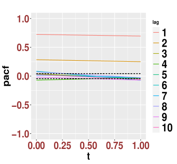
(a) PACFs for model (section.equation).

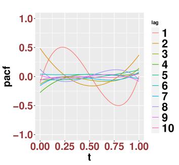
(b) PACFs for model (section.equation).

Figure figure: Typical sample PACF plots (i.e., $\widehat{\rho}_{j}(t)$ in (section.equation)) for models (section.equation) and (section.equation). Here $n=600$ and the plots can be generated using the function $\mathtt{sie.auto.plot}$ from our $\mathtt{R}$ package $\mathtt{Sie2nts}$.

section.subsection.subsubsection Inference of PACFs

In this section, we examine the accuracy and sensitivity of our proposed Algorithm 1 when applied to testing (section.equation) and (section.equation). We first investigate the accuracy. To test (section.equation) for some individual PACF at lag $j$, in the context of (section.equation) and (section.equation), we consider the following four settings: (1). $\delta_{1}=0.5,\delta_{2}=0,$ and $j=2$; (2). $\delta_{1}=0.5,\delta_{2}=0,$ and $j=4$; (3). $\delta_{1}=\delta_{2}=0.3,$ and $j=3;$ (4). $\delta_{1}=\delta_{2}=0.3,$ and $j=5.$ Moreover, to test (section.equation) for the white noise, we consider the following setting in the context of (section.equation) and (section.equation): (5). $\delta_{1}=\delta_{2}=0.$

In Table table, we report the simulated type I error rates for all the above null settings for three different types of basis functions when $n=600.$ We can see that our Algorithm 1 is quite accurate for both tests (section.equation) and (section.equation).

	$\alpha=0.1$					$\alpha=0.05$
Basis/Setting	(1)	(2)	(3)	(4)	(5)	(1)	(2)	(3)	(4)	(5)
	Model (section.equation)
Fourier	0.108	0.096	0.108	0.11	0.098	0.048	0.059	0.061	0.054	0.049
Legendre	0.109	0.1	0.096	0.103	0.108	0.06	0.053	0.055	0.064	0.048
Daubechies-9	0.096	0.102	0.11	0.101	0.095	0.058	0.061	0.054	0.058	0.043
	Model (section.equation)
Fourier	0.098	0.11	0.108	0.099	0.107	0.048	0.062	0.057	0.048	0.039
Legendre	0.103	0.094	0.103	0.095	0.113	0.055	0.053	0.061	0.048	0.053
Daubechies-9	0.093	0.09	0.093	0.104	0.1	0.052	0.058	0.058	0.047	0.046

Table table: Simulated type I error rates. The results are reported based on 1,000 simulations. We can see that our multiplier bootstrap procedure is reasonably accurate for both $\alpha=0.1$ and $\alpha=0.05$. In our $\mathtt{R}$ package $\mathtt{Sie2nts},$ we collect 31 different types basis functions. For visualization of various types of basis functions, we can use the $\mathtt{bs.gene}$ and $\mathtt{bs.plot}$ from our $\mathtt{R}$ package $\mathtt{Sie2nts}.$ The computations of the $p$-values can be obtained directly using the function $\mathtt{auto.pacf.test}$ from the package.

Then we study the power. For definiteness, we report the results for the white noise test that

$$\mathbf{H}_{0}:\ \{x_{i}\}\ \text{is a white noise process}\ \ \text{Vs}\ \ \mathbf{H}_{a}:\ \{x_{i}\}\ \text{is not a white noise process.}$$ (section.equation)

More specifically, in view of the concerned models (section.equation) and (section.equation), $\mathbf{H}_{0}$ in (section.equation) is equivalent to $\delta_{1}=\delta_{2}=0$ while $\mathbf{H}_{a}$ is an AR(1) alternative that $\delta_{2}=0,\delta_{1}>0.$ In Figure figure below, we study the power of our proposed method when $\delta_{1}$ deviates away from zero. We can conclude that our proposed tests are reasonably powerful once the alternative deviates from the null.

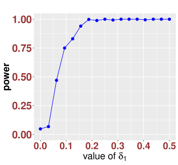
(a) Power for model (section.equation).

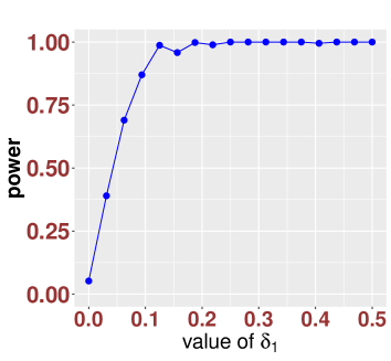
(b) Power for model (section.equation).

Figure figure: Power for models (section.equation) and (section.equation) under the alternative of (section.equation). Here the type I error rate $\alpha=0.05$ and $n=600$. We use the Legendre polynomials as the basis functions and the computations of the $p$-values can be obtained directly using the function $\mathtt{auto.pacf.test}$ from our $\mathtt{R}$ package $\mathtt{Sie2nts}$. The results are reported based 1,000 repetitions.

Finally, for further visualization, using (section.equation) as an example, in Figure figure below, we provide two typical plots of the $p$-values associated with each lag $j$ with (section.equation) under both the null and alternative as in (section.equation). Here for the alternative we set $\delta_{1}=0.5$ and $\delta_{2}=0$ in (section.equation). From the plots we can easily distinguish the null and alternative. Moreover, it is clear that the plots suggest that the null is a white noise process and the alternative is an AR(1) process. Additionally, more simulation results on other types of models can be found in Section D.subsection of our supplement and similar conclusions can also be made.

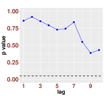
(a) $p$-values under $\mathbf{H}_{0}$ in (section.equation).

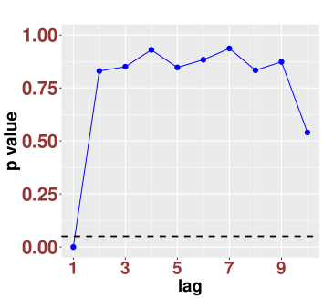
(b) $p$-values under $\mathbf{H}_{a}$ in (section.equation).

Figure figure: Typical $p$-value plots for different lags for model (section.equation) under null and alternative of (section.equation). Here the type one error $\alpha=0.05,$ $n=600$, $\delta_{1}=0.5$ for the alternative. We use the Legendre polynomials as the basis functions and the computations of the $p$-values can be obtained directly using the function $\mathtt{auto.pacf.test}$ from our $\mathtt{R}$ package $\mathtt{Sie2nts}$.

section.subsection Real data analysis

In this section, we apply our methods to the monthly Euro-Dollar exchange rate data set which has also been considered in Killick et al. (2020). The data set can be downloaded from EuroStat at https://ec.europa.eu/eurostat/web/products-datasets/-/ei_mfrt_m. We analyze the exchange rates from January 1999 until October 2017.

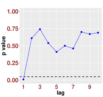
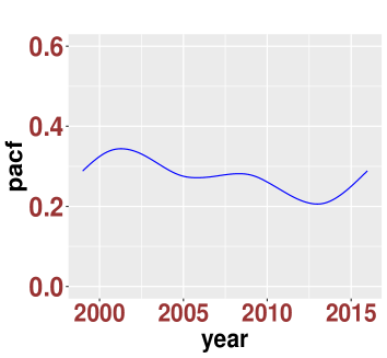
Figure figure: Euro-Dollar exchange rate data. Here we use the Daubechies-9 wavelet as the basis functions. Left panel records the $p$-values associated with different lags and right panel is the estimation of the PACF at the first lag.

Following the traditions of financial data analysis, we consider the log returns of the exchange rate. Moreover, we apply our methods to estimate the PACFs and conduct inference on them. As can be seen from the left panel of Figure figure, based on our inference, a white-noise-driven AR(1) model will be useful to model the data. This agrees with the findings in Killick et al. (2020). In fact, we can conduct the white noise test for the original time series as in (section.equation) using Algorithm 1 and find the $p$-value is $0.013.$ This shows that the time series is not a white noise. Furthermore, after fitting the time series with a time-varying AR(1) model (note that for AR(1) model, the coefficient is identical to $\widehat{\rho}_{1}(t)$), we can conduct the white noise test for the residuals and then find the $p$-value is $0.54$. This confirms that the AR(1) model is likely to be appropriate.

In the right panel of Figure figure, we provide the estimation of the PACF of lag one which is also the coefficient of a time-varying AR(1) model. It can be seen that the even though the PACF is relatively stable, it experiences some smooth changes over time. In fact, one can directly generalize the significance test $T_{1}$ into a test of constancy by considering $T_{1}^{*}:=\int_{0}^{1}[\widehat{\rho}_{1}(t)-\int_{0}^{1}\widehat{\rho}_{1}(s)\mathrm{d}s]^{2}\mathrm{d}t.$ The multiplier bootstrap of $T_{1}^{*}$ yields a $p$-value of $0.031$, indicating that $\rho_{1}(t)$ is likely to be time-varying. This concludes that a locally stationary AR(1) model may be more useful for the model fitting. Due to the pronounced responsiveness of Euro-Dollar exchange rates to the global economy, our plots serve as reasonably accurate reflections of prevailing global economic conditions. For instance, leading up to the global financial crisis (2005-2007), the PACF displays a consistent pattern. Subsequently, from 2008 onwards, there is a gradual decline observed, hitting its lowest point around 2013, coinciding with the recognized period of the financial crisis. Following this, the PACF demonstrates a resurgence. Such a visual representation offers valuable insights into the evolving dynamics of Euro-Dollar exchange rates, aiding in a deeper comprehension of their temporal behavior.

Supplementary file

In the supplement file, we provide the technical proofs, some additional remarks, practical methods for choosing the tuning parameters and additional simulation results.

A Technical proofs

A.subsection Proofs of Section section

In this subsection, we prove Theorem section.thm. The strategies and ideas are similar to those of Theorems 2.4 and 2.11 of Ding & Zhou (2023). We focus on explaining the main differences.

[Proof of Theorem section.thm] For the first part of the proof, it is analogous to the proof of equation (2.6) of Ding & Zhou (2023). We only sketch the proof. Due to similarity, we only prove the first control in (section.equation). Recall (section.equation). Set $\bm{\phi}_{j}(i)=(\phi_{ij,1},\cdots,\phi_{ij,j})^{*}\in\mathbb{R}^{j}.$ It is easy to see from (1) of Assumption section.thm and Yule-Walker’s equation that

$$\bm{\phi}_{j}(i)=\Gamma_{j}^{-1}(i)\bm{\nu}_{j}(i),$$ (A.equation)

where we denoted that

$$\Gamma_{j}(i)=\operatorname{Cov}\left(\bm{x}_{j}(i),\bm{x}_{j}(i)\right)\in\mathbb{R}^{j\times j},\ \bm{\nu}_{j}(i)=\operatorname{Cov}\left(\bm{x}_{j}(i),x_{i}\right)\in\mathbb{R}^{j},$$

where $\bm{x}_{j}(i)=(x_{i-1},\cdots,x_{i-j})\in\mathbb{R}^{j}.$ For the rest of the proof, we can follow lines of that of Theorem 2.4 of Ding & Zhou (2023) verbatim. More specifically, according to (A.equation), we find that in order to study $\rho_{i,j}\equiv\phi_{ij,j},$ it suffices to control the entries of the $j$th row of $\Gamma_{j}^{-1}(i)$ and all the entries of $\bm{\nu}_{j}(i).$ For $\Gamma_{j}^{-1}(i),$ we denote the $j\times j$ symmetric banded matrix $\Gamma_{j}^{s}(i)$ as

$$(\Gamma_{j}^{s}(i))_{kl}=\begin{cases}(\Gamma_{j}(i))_{kl},&|k-l|\leq\frac{j}{K\log j};\\ 0,&\text{otherwise}.\end{cases}$$

Here $K>0$ is some large constant. Using (1) and (2) of Assumption section.thm, by a discussion similar to equation (D.7) of Ding & Zhou (2023), we find that for some constant $C>0$

$$|\rho_{i,j}-\phi_{ij,j}^{s}|\leq Cj^{1-\tau}(K\log j)^{\tau-1},$$

where $\bm{\phi}_{j}(i)^{s}=(\phi_{ij,1}^{s},\cdots,\phi_{ij,j}^{s})^{*}\in\mathbb{R}^{j}$ is defined via $\bm{\phi}_{j}^{s}(i)=(\Gamma_{j}(i)^{s})^{-1}\bm{\nu}_{j}(i).$ Moreover, using (1) of Assumption section.thm, according to the discussions below equation (D.8) of Ding & Zhou (2023), we find that for some constant $C_{1}>0,$

$$|\phi_{ij,j}^{s}|\leq C_{1}(j/(\log j+1))^{-\tau+1}.$$

Combining the above controls, we complete the proof of (section.equation).

For the second part of the proof, for the smoothness that $\rho_{j}(t)\in C^{d}([0,1])$ follows from Lemma 3.1 of Ding & Zhou (2020). To see (section.equation), by (A.equation) and (section.equation), using Cauchy-Schwarz inequality, we have that

$$\left|\bm{\phi}_{j}(i)-\bm{\phi}_{j}(i/n)\right|\leq\left\|\Gamma_{j}^{-1}(i)\right\|\left|\bm{\nu}_{j}(i)-\bm{\nu}_{j}(i/n)\right|+\left\|\Gamma_{j}^{-1}(i)-\Gamma_{j}^{-1}(i/n)\right\|\left|\bm{\nu}_{j}(i/n)\right|.$$ (A.equation)

The rest of the proof follows from the exact reasoning as the arguments of the proof of Theorem 2.11 of Ding & Zhou (2023). In particular, using (1)-(3) of Assumption section.thm, by an argument similar to the equations between (D.31) and (D.32) of Ding & Zhou (2023), we find that the first term of the right-hand side of (A.equation) can be bounded by $\mathrm{O}(j^{1.5}/n)$ and the second term can be bounded by $\mathrm{O}(j^{2}/n).$ This completes our proof.

A.subsection Proofs of Section section

In this subsection, we prove the main results in Section section.

[Proof of Theorem section.thm] The proof is similar to that of Theorem 3.2 of Ding & Zhou (2021). Due to similarity, we only sketch the key points. Similar to (section.equation), we set $\widehat{\bm{\phi}}_{j}(t)$ as the sieve estimator for $\bm{\phi}_{j}(t);$ that is

$$\widehat{\bm{\phi}}_{j}(t):=\widehat{\bm{\beta}}_{j}^{*}\mathbb{B}_{j}(t),\ \mathbb{B}_{j}(t)=\sum_{l=1}^{j}\mathbb{B}_{j,l}(t).$$ (A.equation)

Recall (section.equation). For $1\leq l\leq j,$ denote

$$\bm{\phi}_{j,l}^{(c)}(t)=\sum_{k=1}^{c}a_{jk,l}\alpha_{k}(t),$$

and $\bm{\phi}_{j}^{(c)}=\left(\bm{\phi}_{j,1}^{(c)},\cdots,\bm{\phi}_{j,j}^{(c)}\right)^{*}\in\mathbb{R}^{j}.$ Recall (section.equation). The starting point is the following decomposition

$$\|\widehat{\bm{\phi}}_{j}(t)-\bm{\phi}_{j,j}(t)\|\leq\|\widehat{\bm{\phi}}_{j}(t)-\bm{\phi}^{(c)}_{j,j}(t)\|+|\bm{\phi}_{j,j}(t)-\bm{\phi}_{j,j}^{(c)}(t)|.$$

Since the second term of the right-hand side of the above equation can be bounded by $\mathrm{O}\left(c^{-d}\right)$ using (section.equation), it suffices to control the first term. According to (A.equation), by Cauchy-Schwarz inequality, we see that

$$\|\widehat{\bm{\phi}}_{j,j}(t)-\bm{\phi}^{(c)}_{j,j}(t)\|\leq\sum_{l=1}^{j}\|\widehat{\bm{\phi}}_{j,l}(t)-\bm{\phi}^{(c)}_{j,l}(t)\|\leq\sqrt{j}\zeta_{c}\|\bm{\beta}_{j}-\widehat{\bm{\beta}}_{j}\|.$$ (A.equation)

Moreover, for the OLS estimation, we have that

$$\bm{\beta}_{j}-\widehat{\bm{\beta}}_{j}=n(Y_{j}^{*}Y_{j})^{-1}\frac{Y_{j}^{*}\bm{\epsilon}_{j}}{n},$$ (A.equation)

where $\bm{\epsilon}_{j}=(\epsilon_{j+1,j}+\mathfrak{r},\cdots,\epsilon_{n,j}+\mathfrak{r})^{*}\in\mathbb{R}^{n-j}$ with $\mathfrak{r}$ representing the error term in (section.equation). The rest of the discussions follow lines of that of Theorem 3.2 of Ding & Zhou (2021).

To control the right-hand side of (A.equation), first, by an argument similar to (A.9) of Ding & Zhou (2021), for $\Sigma^{(j)}$ defined in (section.equation), we find that

$$\left\|\frac{1}{n}Y_{j}^{*}Y_{j}-\Sigma^{(j)}\right\|=\mathrm{O}_{\mathbb{P}}\left(jc\left(\frac{\xi_{c}^{2}}{\sqrt{n}}+\frac{\xi_{c}^{2}n^{\frac{2}{\tau+1}}}{n}\right)\right).$$

Combining the above discussion, together with Assumption section.thm and the assumption of (section.equation), we see that

$$\left\|n(Y_{j}^{*}Y_{j})^{-1}\right\|=\mathrm{O}_{\mathbb{P}}(1).$$ (A.equation)

Second, according to a discussion similar to (A.12) of Ding & Zhou (2021) and the fact that $\mathfrak{r}=\mathrm{O}_{\mathbb{P}}(j^{2}/n+jc^{-d})$, we have that

$$\left\|\frac{Y_{j}^{*}\bm{\epsilon}_{j}}{n}\right\|=\mathrm{O}_{\mathbb{P}}\left(\xi_{c}\left(1+\frac{j^{2}}{n}+jc^{-d}\right)\sqrt{\frac{jc}{n}}\right).$$ (A.equation)

We point out that the error rate $j^{2}/n$ is faster than the $j^{2.5}/n$ in (A.12) of Ding & Zhou (2021) or (2.23) and (2.24) of Ding & Zhou (2023) because of the assumption that $\{x_{i}\}$ is a mean-zero time series. Inserting the above two bounds into (A.equation), we conclude that

$$\|\bm{\beta}_{j}-\widehat{\bm{\beta}}_{j}\|=\mathrm{O}_{\mathbb{P}}\left(\xi_{c}\left(1+\frac{j^{2}}{n}+jc^{-d}\right)\sqrt{\frac{jc}{n}}\right).$$

Combining (A.equation), we can conclude our proof.

[Proof of Theorem section.thm] The proof follows from lines of those of Proposition 3.7 of Ding & Zhou (2023) verbatim. We omit the details.

[Proof of Theorem section.thm] The proof of part 1 follows from lines of those of Proposition 3.7 of Ding & Zhou (2023) verbatim. We omit the details.

For part 2, we start with (section.equation). Before proceeding to the actual proof, we first explore the relation between $\rho_{k}(t)$ and $\phi_{\mathsf{h},k}(t)$ for $1\leq k\leq\mathsf{h}$ under the null hypothesis of (section.equation). First of all, under (section.equation), according to Theorem section.thm, we can conclude that

$$\rho_{i,\mathsf{h}}\equiv\phi_{i\mathsf{h},\mathsf{h}}=\mathrm{O}\left(\min\left\{\frac{\mathsf{h}^{2}}{n},\left(\frac{\log\mathsf{h}+1}{\mathsf{h}}\right)^{\tau-1}\right\}\right).$$ (A.equation)

Combining with an argument similar to Theorem 2.11 of Ding & Zhou (2023) and the smoothness of $\phi_{\mathsf{h},\mathsf{h}}(t)$, we can conclude that for all $0\leq t\leq 1$

$$\phi_{\mathsf{h},\mathsf{h}}(t)=\mathrm{O}\left(\frac{\mathsf{h}^{2}}{n}\right).$$ (A.equation)

Then with an argument similar to Theorem 2.11 of Ding & Zhou (2023), in light of the representation (section.equation), we see that

$$x_{i}=\sum_{j=1}^{\mathsf{h}-1}\phi_{\mathsf{h},j}\left(\frac{i}{n}\right)x_{i-j}+\epsilon_{i,\mathsf{h}}+\mathrm{O}_{\mathbb{P}}\left(\frac{\mathsf{h}^{2}}{n}\right).$$

Therefore, we can repeat (A.equation) and (A.equation) to get that

$$\phi_{\mathsf{h},k}(t)=\mathrm{O}\left(\frac{k^{2}}{n}\right),\ 1\leq k\leq\mathsf{h},$$ (A.equation)

and conclude that

$$x_{i}=\epsilon_{i,\mathsf{h}}+\mathrm{O}_{\mathbb{P}}\left(\frac{\mathsf{h}^{3}}{n}\right).$$

Using our assumptions on $\mathsf{h}$, we find that the error term of the above approximation is always negligible with high probability. With the above preparation, we proceed to the proof. By definition, we have that

$$T_{\text{BP}}-T_{2}=\sum_{k=1}^{\mathsf{h}}\int_{0}^{1}\left(\widehat{\rho}_{k}^{2}(t)-\widehat{\phi}_{\mathsf{h},k}^{2}(t)\right)\mathrm{d}t.$$

By a discussion similar to Theorem section.thm, we have that (see Theorem 3.3 of Ding & Zhou (2020)) for $1\leq k\leq\mathsf{h}$

$$\phi_{\mathsf{h},k}(t)=\widehat{\phi}_{\mathsf{h},k}(t)+\mathrm{O}_{\mathbb{P}}\left(\Psi(\mathsf{h},c)\right),$$

where we recall (section.equation). Combining the above controls with Theorem section.thm, under the null hypothesis (section.equation), we see that

$$\widehat{\rho}_{k}^{2}(t)=\mathrm{O}_{\mathbb{P}}\left(\Psi^{2}(k,c)\right),\ \widehat{\phi}_{\mathsf{h},k}^{2}(t)=\mathrm{O}_{\mathbb{P}}\left(\frac{k^{4}}{n^{2}}+\Psi^{2}(\mathsf{h},c)\right).$$

Consequently, we have that

$$T_{\text{BP}}-T_{2}=\mathrm{O}_{\mathbb{P}}\left(\mathsf{h}\Psi^{2}(\mathsf{h},c)+\frac{\mathsf{h}^{5}}{n^{2}}+\sum_{k=1}^{\mathsf{h}}\Psi^{2}(k,c)\right).$$

Then, for (section.equation), using the definition of $g_{k}$ in (section.equation) and the fact that $g_{2}\asymp\sqrt{\mathsf{h}c},$ the proof follows from (section.equation), (section.equation) and the assumption of (section.equation).

Finally, for part 3, by a discussion similar to (A.equation) and (A.equation), we find that (section.equation) yields that

$$\sum_{k=1}^{\mathsf{h}}\int_{0}^{1}\phi_{\mathsf{h},k}^{2}(t)\mathrm{d}t>C_{\alpha}\frac{\sqrt{\mathsf{h}c}}{n}.$$

Then the proof follows from lines of those of Proposition 3.7 of Ding & Zhou (2023) verbatim.

[Proof of Corollary section.thm] The proof follows directly from the proof of Theorem 3.10 of Ding & Zhou (2023) by setting $b_{*}=\mathsf{h}$ therein.

A.subsection Additional assumptions

In this section, we collect some more assumptions and provide more discussions on these technical assumptions. The following assumption will be needed in our proof. It is a mild assumption and can be easily satisfied by many time series. We refer the readers to Section C.1 of Ding & Zhou (2023) for more details.

Assumption A.thm.

We assume the following assumptions hold true

1. Suppose $\tau>4.5$ in Assumption section.thm. Moreover, we assume that $c$ is of the form (section.equation) and satisfies that for large constant $C>0$

   $$\frac{C}{\tau}+a<1,\ \operatorname{and}\ da>2.$$

2. We assume that the derivatives of $\gamma(t,j)$ decay with $j$ as follows

   $$\sup_{t\in[0,1]}\sum_{j=0}^{\infty}|\gamma^{(d)}(t,j)|<\infty,$$

   where $\gamma^{(d)}(t,j)$ is the d$th$ derivative of $\gamma(t,j)$ with respect to $t$.

3. There exist constants $\omega_{1},\omega_{2}\geq 0,$ for some constant $C>0,$ we have

   $$\sup_{t}|\nabla\mathbf{B}(t)|\leq Cn^{\omega_{1}}c^{\omega_{2}}.$$

B Additional remarks and examples

In this section, we provide several remarks and examples. The following remark provides more discussions on Theorem section.thm.

Remark B.thm.

Theorem section.thm is established for locally stationary time series as in Definition section.thm where an exact cut-off is not available in general. An exception is the locally stationary AR(p) process as in Zhou (2013b), where

$$x_{i}=\phi_{0}(i/n)+\sum_{j=1}^{p}\phi_{j}(i/n)x_{i-j}+\epsilon_{i},$$ (B.equation)

where $\{\epsilon_{i}\}$ is a time-varying white noise process. In this setting, it is clear that

$$\rho_{i,j}=\begin{cases}\phi_{j}(i/n),&j=p;\\ 0,&j>p,\end{cases}$$

so that $(\ref{eq_decayrate})$ and (section.equation) holds trivially once $p$ is fixed or divergent slowly. In fact, as proved in Theorem 2.11 of Ding & Zhou (2023), any locally stationary time series satisfying Definition section.thm and Assumption section.thm can be always well approximated by a time series in the form of (B.equation) with slowly diverging $p.$ In this regard, our results can be used to provide an order for the AR approximation; see Remark B.thm below.

The following remark provides more explanations on the conditions in Assumption section.thm.

Remark B.thm.

The conditions (1)–(3) in Assumption section.thm are mild and commonly used in the literature. First, (1) is introduced to avoid the erratic behavior of the time series and frequently used in the statistics literature involving the covariance and precision matrix estimation Cai et al. (2016); Chen et al. (2013); Ding & Zhou (2020, 2023); Yuan (2010). Moreover, as proved in (Ding & Zhou, 2023, Proposition 2.9), it is equivalent to the uniform positiveness of the local spectral density function of $\{x_{i}\}.$ Second, (2) imposes the condition that the temporal structure of $\{x_{i}\}$ decays polynomially fast. This amounts to a short range dependent requirement for $\{x_{i}\}$ when $\tau>1.$ Analogous results can be easily obtained for the exponentially decay setting where

$$\max_{k,n}\left|\operatorname{Cov}(x_{k,n},x_{k+r,n})\right|\leq Ca^{|r|},\ \text{for some}\ 0<a<1.$$

Third, (3) requires that the autocovariance functions of $\{x_{i}\}$ are smooth so that its PACFs can be estimated consistently. It is commonly used in the literature of locally stationary time series Dahlhaus (2012); Dahlhaus et al. (2019); Ding & Zhou (2020, 2023); Zhou & Wu (2009).

The remark below provides some insights on how to use our results to estimate the order of a locally stationary AR process.

Remark B.thm.

We discuss how to generalize the use of PACFs of stationary AR process to locally stationary AR process. For definiteness, we focus on the following time-varying AR($p$) process which has been used in Zhou (2013b); Dahlhaus et al. (2019)

$$x_{i}=\sum_{j=1}^{p}\phi_{j}(i/n)x_{i-j}+\epsilon_{i},$$ (B.equation)

where $\{\epsilon_{i}\}$ is some locally-stationary white noise process and $\phi_{j}(\cdot),j=0,1,2,\cdots,p,$ are some smooth functions on $[0,1]$. Before estimating these time-varying coefficients, we first need to provide an estimator for $p.$ Here $p$ is allowed to diverge with $n.$ Based on the results of Theorem section.thm, inspired by the ideas in Ding & Yang (2022); Ding et al. (2023), we can propose a sequential test estimate based on the following hypothesis testing problem

$$\mathbf{H}_{0}:p=p_{0}\ \text{vs}\ \mathbf{H}_{a}:p_{0}<p\leq p_{*},$$ (B.equation)

where $p_{0}$ is some pre-given integer representing our belief of the true value of $p$ and $p_{*}$ is some large integer that is interpreted as the maximum possible order the model can have. In light of (section.equation), we can use the following estimate

$$\widetilde{p}=\max\{1\leq j\leq p_{*}:\ \mathbf{H}_{a1}\ \text{in}\ (\ref{eq_firstnull})\ \text{is accepted}\}.$$ (B.equation)

The following remark is related to the hypothesis testing (section.equation).

Remark B.thm.

Two remarks are in order. First, in classic stationary time series analysis, in addition to Box-Pierce test, people also use the Ljung–Box (LB) test Ljung & Box (1978). Moreover, the BP and LB tests are asymptotic equivalent and follow the Chi-squared distribution with the same degree of freedom $\mathsf{h}$. In this regard, we can also modify the LB test using

$$\mathcal{Q}_{\text{MLB}}:=n(n+2)\sum_{k=1}^{\mathsf{h}}\frac{\int_{0}^{1}\widehat{\rho}_{k}(t)^{2}}{n-k}.$$

Moreover, we can study such a modified statistic as Theorem section.thm. Due to the asymptotic equivalence, we omit further details. Second, (section.equation) is frequently used for model diagnostics. In this regard, it provides an alternative approach to choose the order of AR approximations by checking whether the residuals follow white noise after fitting some AR models.

Finally, we provide two frequently-used models of locally stationary time series in the literature and explain how Definition section.thm and Assumption section.thm can be easily satisfied.

Example B.thm.

We shall first consider the locally stationary time series model in Zhou & Wu (2009, 2010) using a physical representation so that

$$x_{i,n}=G_{n}(\frac{i}{n},\mathcal{F}_{i}),\ i=1,2,\cdots,n,$$ (B.equation)

where $\mathcal{F}_{i}=(\cdots,\eta_{i-1},\eta_{i})$ and $\eta_{i},\ i\in\mathbb{Z}$ are i.i.d centered random variables, and $G_{n}:[0,1]\times\mathbb{R}^{\infty}\rightarrow\mathbb{R}$ is a measurable function such that $\xi_{i,n}(t):=G_{n}(t,\mathcal{F}_{i})$ is a properly defined random variable for all $t\in[0,1].$ In (B.equation), by allowing the data generating mechanism $G_{n}$ depending on the time index $t$ in such a way that $G_{n}(t,\mathcal{F}_{i})$ changes smoothly with respect to $t$, one has local stationarity in the sense that the subsequence $\{x_{i,n},...,x_{i+j-1,n}\}$ is approximately stationary if its length $j$ is sufficiently small compared to $n$. Moreover, they quantify the temporal decay using the physical dependence measure for (B.equation) as follows

$$\delta(j,q):=\sup_{t\in[0,1]}||G_{n}(t,\mathcal{F}_{0})-G_{n}(t,\mathcal{F}_{0,j})||_{q}.$$ (B.equation)

Moreover, the following assumptions are needed to ensure local stationarity.

Assumption B.thm.

$G_{n}(\cdot,\cdot)$ defined in (B.equation) satisfies the property of stochastic Lipschitz continuity, i.e., for some $q>2$ and $C>0,$

$$\left|\left|G_{n}(t_{1},\mathcal{F}_{i})-G_{n}(t_{2},\mathcal{F}_{i})\right|\right|_{q}\leq C|t_{1}-t_{2}|,$$ (B.equation)

where $t_{1},t_{2}\in[0,1].$ Furthermore,

$$\sup_{t\in[0,1]}\max_{1\leq i\leq n}||G_{n}(t,\mathcal{F}_{i})||_{q}<\infty.$$ (B.equation)

It can be shown that time series $\{x_{i,n}\}$ with physical representation (B.equation) and Assumption B.thm satisfies Definition section.thm. In particular, for each fixed $t\in[0,1],$ $\gamma(t,j)$ in Definition section.thm can be found easily using the following

$$\gamma(t,j)=\operatorname{Cov}(G_{n}(t,\mathcal{F}_{0}),G_{n}(t,\mathcal{F}_{j})).$$ (B.equation)

Note that the assumptions (B.equation) and (B.equation) ensure that $\gamma(t,j)$ is Lipschiz continuous in $t$. Moreover, for each fixed $t,$ $\gamma(t,\cdot)$ is the autocovariance function of $\{G_{n}(t,\cdot)\},$ which is a stationary process.

The physical representation form (B.equation) includes many commonly used locally stationary time series models. For example, let $\{z_{i}\}$ be zero-mean i.i.d. random variables (or a white noise) with variance $\sigma^{2}$. We also assume $a_{j,n}(\cdot),j=0,1,\cdots$ be $C^{d}([0,1])$ functions such that

$$G_{n}(t,\mathcal{F}_{i})=\sum_{k=0}^{\infty}a_{k,n}(t)z_{i-k}.$$ (B.equation)

(B.equation) is a locally stationary linear process. It is easy to see that (2) and (3) of Assumption section.thm will be satisfied if $\sup_{t\in[0,1]}|a_{j,n}(t)|\leq Cj^{-\tau},\ j\geq 1;\ \sum_{j=0}^{\infty}\sup_{t\in[0,1]}|a_{j,n}^{\prime}(t)|<\infty,$ and

$$\sup_{t\in[0,1]}|a_{j,n}^{(d)}(t)|\leq Cj^{-\tau},\ j\geq 1.$$ (B.equation)

Furthermore, we note that the local spectral density function of (B.equation) can be written as $f(t,w)=\sigma^{2}|\psi(t,e^{-\mathrm{i}j\omega})|^{2},$ where $\psi(\cdot,\cdot)$ is defined such that $G_{n}(t,\mathcal{F}_{i})=\psi(t,B)z_{i}$ with $B$ being the backshift operator. As discussed in Remark B.thm, (1) of Assumption B.equation will be satisfied if $|\psi(t,e^{-\mathrm{i}j\omega})|^{2}\geq\kappa$ for all $t$ and $\omega,$ where $\kappa>0$ is some universal constant. For more examples of locally stationary time series in the form of (B.equation) especially nonlinear time series, we refer the readers to Wu (2005), (Ding & Zhou, 2020, Section 2.1) , (Dahlhaus et al., 2019, Example 2.2 and Proposition 4.4), (Karmakar et al., 2022, Proposition E.6) and Ding & Zhou (2021); Karmakar et al. (2022); Mayer et al. (2020). Especially, the time-varying AR and ARCH models can be written into (B.equation) asymptotically Ding & Zhou (2023), and Assumptions section.thm and B.thm can be easily satisfied under mild assumptions. We refer the readers to the aforementioned references for more details.

For a second example, note that in Dahlhaus & Rao (2006); Dette et al. (2011); Vogt (2012), the locally stationary time series is defined as follows (see Definition 2.1 of Vogt (2012)). $\{x_{i,n}\}$ is locally stationary time series if for each scaled time point $u\in[0,1],$ there exists a strictly stationary process $\{h_{i,n}(u)\}$ such that

$$|x_{i,n}-h_{i,n}(u)|\leq\left(|t_{i}-u|+\frac{1}{n}\right)U_{i,n}(u),\ \text{a.s},$$ (B.equation)

where $U_{i,n}(u)\in L^{q}([0,1])$ for some $q>0.$ By similar arguments as those of model (B.equation) Ding & Zhou (2023), Definition section.thm as well as assumptions of this subsection can be verified for (B.equation), especially (B.equation) implies (section.equation).

C Tuning parameters selection

In this section, we explain how to choose the tuning parameters associated with our proposed methodology.

First, we discuss how to choose the tuning parameters $c$ and $m$ used in Algorithm 1. We use a data-driven procedure proposed in Bishop (2013) to choose $c.$ For a given integer $l,$ say $l=\lfloor 3\log_{2}n\rfloor,$ we divide the time series into two parts: the training part $\{x_{i}\}_{i=1}^{n-l}$ and the validation part $\{x_{i}\}_{i=n-l+1}^{n}.$ With some preliminary initial value $c$, we propose a sequence of candidates $c_{j},\ j=1,2,\cdots,v,$ in an appropriate neighborhood of $c$ where $v$ is some given integer. For each of the choices $c_{j},$ we fit a time-varying AR($h_{2}$) model as in (section.equation) with $c_{j}$ sieve basis expansion using the training data set. Then using the fitted model, we forecast the time series in the validation part of the time series. Let $\widehat{x}_{n-l+1,j},\cdots,\widehat{x}_{n,j}$ be the forecast of $x_{n-l+1},...,x_{n},$ respectively using the parameter $c_{j}$. Then we choose the parameter $c_{j_{0}}$ with the minimum sample MSE of forecast, i.e.,

$${j_{0}}:=\operatorname*{argmin}_{(j:1\leq j\leq v)}\frac{1}{l}\sum_{k=n-l+1}^{n}(x_{k}-\widehat{x}_{k,j})^{2}.$$

To choose an $m$ for practical implementation, in Zhou (2013a), the author used the minimum volatility (MV) method to choose the window size $m$ for the scalar covariance function. The MV method does not depend on the specific form of the underlying time series dependence structure and hence is robust to misspecification of the latter structure Politis et al. (1999). The MV method utilizes the fact that the covariance structure of $\widehat{\Pi}$ becomes stable when the block size $m$ is in an appropriate range, where $\widehat{\Pi}=E[\widehat{\Phi}\widehat{\Phi}^{*}|(x_{1},\cdots,x_{n})]$ is defined as

$$\widehat{\Pi}:=\frac{1}{(n-m-h_{2}+1)m}\sum_{i=h_{2}+1}^{n-m}\Big{[}\Big{(}\sum_{j=i}^{i+m}\widehat{\bm{w}}_{h_{2},j}\Big{)}\otimes\Big{(}\mathbf{B}(\frac{i}{n})\Big{)}\Big{]}\times\Big{[}\Big{(}\sum_{j=i}^{i+m}\widehat{\bm{w}}_{h_{2},j}\Big{)}\otimes\Big{(}\mathbf{B}(\frac{i}{n})\Big{)}\Big{]}^{*}.$$ (C.equation)

Therefore, it desires to minimize the standard errors of the latter covariance structure in a suitable range of candidate $m$’s. In detail, for a give large value $m_{n_{0}}$ and a neighborhood control parameter $h_{0}>0,$ we can choose a sequence of window sizes $m_{-h_{0}+1}<\cdots<m_{1}<m_{2}<\cdots<m_{n_{0}}<\cdots<m_{n_{0}+h_{0}}$ and obtain $\widehat{\Pi}_{m_{j}}$ by replacing $m$ with $m_{j}$ in (C.equation), $j=-h_{0}+1,2,\cdots,n_{0}+h_{0}.$ For each $m_{j},j=1,2,\cdots,m_{n_{0}},$ we calculate the matrix norm error of $\widehat{\Omega}_{m_{j}}$ in the $h_{0}$-neighborhood, i.e.,

$$\mathsf{se}(m_{j}):=\mathsf{se}(\{\widehat{\Pi}_{m_{j+k}}\}_{k=-h_{0}}^{h_{0}})=\left[\frac{1}{2h_{0}}\sum_{k=-h_{0}}^{h_{0}}\|\overline{\widehat{\Pi}}_{m_{j}}-\widehat{\Pi}_{m_{j}+k}\|^{2}\right]^{1/2},$$

where $\overline{\widehat{\Pi}}_{m_{j}}=\sum_{k=-h_{0}}^{h_{0}}\widehat{\Pi}_{m_{j}+k}/(2h_{0}+1).$ Therefore, we choose the estimate of $m$ using

$$\widehat{m}:=\operatorname*{argmin}_{m_{1}\leq m\leq m_{n_{0}}}\mathsf{se}(m).$$

Note that in Zhou (2013a) the author used $h_{0}=3$ and we also adopt this choice in the current paper.

Second, we discuss how to choose a large value of $\mathsf{h}$ to construct the statistic $T_{2}$ in (section.equation). Theoretically, the lower bound for the order of $\mathsf{h}$ is given by $j^{*}$ as in (section.equation), while the upper bound is provided in the assumption of (section.equation). The lower bound yields that for all $j\geq\mathsf{h},$ $\sup_{t}\rho_{j}(t)=\mathrm{o}(n^{-1/2}),$ while the upper bound guarantees that the error term is negligible. To balance these two conditions, for practical implementation, we use the following value

$$\mathsf{h}:=\min\left\{1\leq j\leq\mathsf{h}^{*}:\ \mathbf{H}_{01}\ \text{in}\ (\ref{eq_firstnull})\ \text{is accepted}\right\},$$

where $\mathsf{h}^{*}>0$ is some pre-given large value (say, $\mathsf{h}^{*}=50$). We emphasize that this can be easily done using our $\mathtt{R}$ package $\mathtt{Sie2nts}$ by generating a plot as in Figure figure.

D Additional simulation results

In this section, we provide additional numerical simulation results.

D.subsection More results on other types of models

In this section, we conduct more numerical simulations using both stationary and non-stationary MA(1) models. For some constant $\delta\in[0,0.5],$ we consider the stationary MA(1) process

$$x_{i}=\epsilon_{i}+\delta\epsilon_{i-1},$$ (D.equation)

and the locally stationary MA(1) process

$$x_{i}=\epsilon_{i}+\delta\sin(2\pi i/n)\epsilon_{i-1},$$ (D.equation)

where $\epsilon_{i},1\leq i\leq n,$ are i.i.d. standard Gaussian random variables. Note that when $\delta=0$ in (D.equation) and (D.equation), they both reduce to the standard white noise. Since (D.equation) and (D.equation) are essentially AR($\infty$) models, one can follow the discussions of Section 3.3 of Shumway & Stoffer (2017) to calculate the true PACFs.

For the estimation of the PACFs, in Figure A, we provide the plots of the PACFs of the first 10 lags for both (D.equation) and (D.equation). We can see that our estimates are reasonably accurate. Regarding the inference of the PACFs, for the purpose of definiteness, we focus on the white noise test (section.equation) where $\mathbf{H}_{0}$ corresponds to $\delta=0$ in (D.equation) and (D.equation) and $\mathbf{H}_{a}$ corresponds to an MA(1) alternative that $\delta>0.$ Under $\mathbf{H}_{0},$ (D.equation) and (D.equation) are essentially the same model. For $n=600,$ under the type I error rate $\alpha=0.05,$ the simulated type I error rates are $0.047,0.051,0.056$ for the Fourier, Legendre and Daubechies-9 basis functions, respectively based on 1,000 repetitions. This shows the accuracy of our test. To examine the power, in Figure B, we report how the simulated power changes when $\delta$ deviates away from zero. We can conclude that our proposed test is reasonably powerful once the alternative deviates from the null.

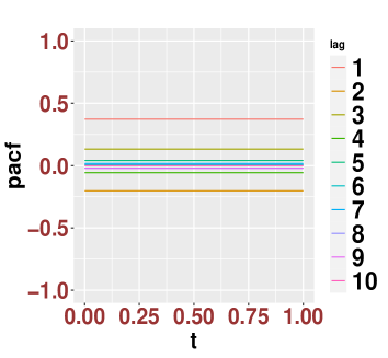
(a) PACFs for model (D.equation).

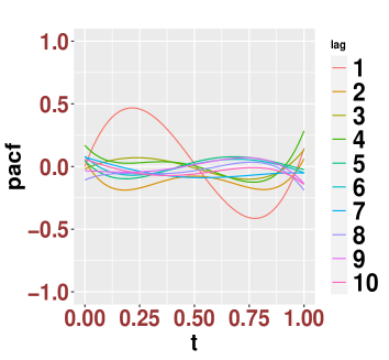
(b) PACFs for model (D.equation).

Figure A: PACF plots for models (D.equation) and (D.equation). Here $n=600.$

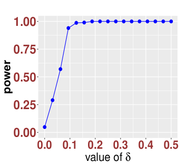
(a) Power for model (D.equation).

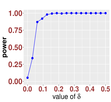
(b) Power for model (D.equation).

Figure B: Power for models (D.equation) and (D.equation) under the alternative of (section.equation). Here the type I error rate $\alpha=0.05$ and $n=600$. We use the Legendre polynomials as the basis functions. The results are reported based 1,000 repetitions.

D.subsection Comparison with Killick et al. (2020) on estimating the PACFs

In this section, we compare our method with the ones proposed in Killick et al. (2020) in terms of the estimation of the PACFs using the mean integrated squared error (MISE). To implement Killick et al. (2020), we use the $\mathtt{R}$ package $\mathtt{lpacf}$ which is developed by the authors of Killick et al. (2020).

For definiteness, we consider the AR type models (section.equation) and (section.equation) with $\delta_{1}=0.5$ and $\delta_{2}=0.$ Consequently, for model (section.equation), the true PACFs are

$$\rho_{j}(t)\equiv\begin{cases}0.5&j=1\\ 0&j\geq 2\end{cases},$$

and for model (section.equation), the true PACFs are

$$\rho_{j}(t)=\begin{cases}0.5\sin(2\pi t)&j=1\\ 0&j\geq 2\end{cases}.$$

Let $\widehat{\rho}_{j}(t)$ be some estimator for $\rho_{j}(t),$ the MISE is defined as

$$\mathsf{MISE}(j)=\int_{0}^{1}(\widehat{\rho}_{j}(t)-\rho_{j}(t))^{2}\mathrm{d}t.$$

In the actual calculations, MISE can be well approximated by an Riemann summation. In Table A, we record the $\mathsf{MISE}(j),j=1,2,3,4,$ for our proposed method (denoted as Proposed) and the two methods in Killick et al. (2020) (the wavelet-based method is denoted as Lpacf-I and the Epanechnikov windowed method is denoted as Lpacf-II). We can conclude that our proposed method has better finite sample performance than Killick et al. (2020) which are known to have worse performance near the boundaries.

Methods/Lags	$j=1$	$j=2$	$j=3$	$j=4$
	Model (section.equation)
Proposed	$8\times 10^{-4}$	$7\times 10^{-4}$	$3\times 10^{-3}$	$1\times 10^{-3}$
Lpacf-I	$9\times 10^{-3}$	$7\times 10^{-3}$	$9\times 10^{-3}$	$7\times 10^{-3}$
Lpacf-II	0.042	0.054	0.043	0.051
	Model (section.equation)
Proposed	$9.8\times 10^{-3}$	$1.9\times 10^{-3}$	$2.5\times 10^{-3}$	$2.7\times 10^{-3}$
Lpacf-I	0.016	$7.5\times 10^{-3}$	$3.5\times 10^{-3}$	$4\times 10^{-3}$
Lpacf-II	0.049	0.051	0.042	0.055

Table A: Comparison of the accuracy of the estimation of PACFs using MISE. Here Proposed stands for our estimator (section.equation) and Lpacf-I and Lpacf-II are the two methods introduced in Killick et al. (2020). Our proposed method can be implemented using our package $\mathtt{Sie2nts}$ and Lpacf-I/II can be implemented using the package $\mathtt{lpacf}.$ Here $n=1024.$

References

- Bishop (2013) Bishop, C. (2013). Pattern Recognition and Machine Learning. Information science and statistics. Springer.
- Box & Pierce (1970) Box, G. E. & Pierce, D. A. (1970). Distribution of residual autocorrelations in autoregressive-integrated moving average time series models. Journal of the American statistical Association 65, 1509–1526.
- Brockwell & Davis (1987) Brockwell, P. & Davis, R. (1987). Time series: Theory and Methods. Springer-Verlag.
- Cai et al. (2016) Cai, T. T., Liu, W. & Zhou, H. H. (2016). Estimating sparse precision matrix: Optimal rates of convergence and adaptive estimation. Ann. Statist. 44, 455–488.
- Chen (2007) Chen, X. (2007). Large sample sieve estimation of semi-nonparametric models. Handbook of econometrics 6, 5549–5632.
- Chen et al. (2013) Chen, X., Xu, M. & Wu, W. B. (2013). Covariance and precision matrix estimation for high-dimensional time series. Ann. Statist. 41, 2994–3021.
- Dahlhaus (2012) Dahlhaus, R. (2012). Locally stationary processes. In Handbook of statistics, vol. 30. Elsevier, pp. 351–413.
- Dahlhaus & Rao (2006) Dahlhaus, R. & Rao, S. S. (2006). Statistical inference for time-varying arch processes. The Annals of Statistics 34, 1075–1114.
- Dahlhaus et al. (2019) Dahlhaus, R., Richter, S. & Wu, W. B. (2019). Towards a general theory for nonlinear locally stationary processes. Bernoulli 25, 1013–1044.
- Dette et al. (2011) Dette, H., Preubb, P. & Vetter, M. (2011). A measure of stationarity in locally stationary processes with applications to testing. J. Am. Stat. Assoc. 106, 1113–1124.
- Dette & Wu (2020) Dette, H. & Wu, W. (2020). Prediction in locally stationary time series. Journal of Business & Economic Statistics , 1–12.
- Ding et al. (2023) Ding, X., Xie, J., Yu, L. & Zhou, W. (2023). Extreme eigenvalues of sample covariance matrices under generalized elliptical models with applications. arXiv preprint arXiv:2303.03532 .
- Ding & Yang (2022) Ding, X. & Yang, F. (2022). Tracy-Widom distribution for heterogeneous gram matrices with applications in signal detection. IEEE Transactions on Information Theory 68, 6682–6715.
- Ding & Zhou (2020) Ding, X. & Zhou, Z. (2020). Estimation and inference for precision matrices of nonstationary time series. Ann. Statist. 48, 2455–2477.
- Ding & Zhou (2021) Ding, X. & Zhou, Z. (2021). Simultaneous sieve inference for time-inhomogeneous nonlinear time series regression. arXiv preprint arXiv:2112.08545 .
- Ding & Zhou (2023) Ding, X. & Zhou, Z. (2023). Auto-regressive approximations to non-stationary time series, with inference and applications. The Annals of Statistics 51, 1207 – 1231.
- Ding & Zhou (2024) Ding, X. & Zhou, Z. (2024). Supplement to ”On the partial autocorrelation function for locally stationary time series: characterization, estimation and inference” .
- Dégerine & Lambert-Lacroix (2003) Dégerine, S. & Lambert-Lacroix, S. (2003). Characterization of the partial autocorrelation function of nonstationary time series. Journal of Multivariate Analysis 87, 46–59.
- Goerg (2012) Goerg, G. M. (2012). Testing for white noise against locally stationary alternatives. Statistical Analysis and Data Mining: The ASA Data Science Journal 5, 478–492.
- Karmakar et al. (2022) Karmakar, S., Richter, S. & Wu, W. B. (2022). Simultaneous inference for time-varying models. Journal of Econometrics 227, 408–428.
- Killick et al. (2020) Killick, R., Knight, M. I., Nason, G. P. & Eckley, I. A. (2020). The local partial autocorrelation function and some applications. Electronic Journal of Statistics 14, 3268 – 3314.
- Kley et al. (2019) Kley, T., Preuß, P. & Fryzlewicz, P. (2019). Predictive, finite-sample model choice for time series under stationarity and non-stationarity. Electronic Journal of Statistics 13, 3710–3774.
- Ljung & Box (1978) Ljung, G. M. & Box, G. E. (1978). On a measure of lack of fit in time series models. Biometrika 65, 297–303.
- Mayer et al. (2020) Mayer, U., Zähle, H. & Zhou, Z. (2020). Functional weak limit theorem for a local empirical process of non-stationary time series and its application. Bernoulli 26, 1891–1911.
- Politis et al. (1999) Politis, D., Wolf, D., Romano, J., Wolf, M., Bickel, P., Diggle, P. & Fienberg, S. (1999). Subsampling. Springer Series in Statistics. Springer New York.
- Ramsey (1974) Ramsey, F. L. (1974). Characterization of the partial autocorrelation function. The Annals of Statistics , 1296–1301.
- Roueff & Sanchez-Perez (2018) Roueff, F. & Sanchez-Perez, A. (2018). Prediction of weakly locally stationary processes by auto-regression. Lat. Am. J. Probab. Math. Stat. 15, 1215–1239.
- Shumway & Stoffer (2017) Shumway, R. & Stoffer, D. (2017). Time Series Analysis and Its Applications: With R Examples. Springer Texts in Statistics. Springer International Publishing, 4th ed.
- Vogt (2012) Vogt, M. (2012). Nonparametric regression for locally stationary time series. Ann. Statist. 40, 2601–2633.
- Wu (2005) Wu, W. (2005). Nonlinear system theory: Another look at dependence. Proc Natl Acad Sci U S A. 40, 14150–14151.
- Yuan (2010) Yuan, M. (2010). High dimensional inverse covariance matrix estimation via linear programming. J. Mach. Learn. Res. 11, 2261–2286.
- Zhou (2013a) Zhou, Z. (2013a). Heteroscedasticity and autocorrelation robust structural change detection. J. Am. Stat. Assoc. 108, 726–740.
- Zhou (2013b) Zhou, Z. (2013b). Inference for non-stationary time-series autoregression. Journal of Time Series Analysis 34, 508–516.
- Zhou & Wu (2009) Zhou, Z. & Wu, W. (2009). Local linear quantile estimation for non-stationary time series. Ann. Stat. 37, 2696–2729.
- Zhou & Wu (2010) Zhou, Z. & Wu, W. (2010). Simultaneous inference of linear models with time varying coefficents. J.R. Statist. Soc. B 72, 513–531.