Bayesian Nonparametrics Meets Data-Driven Robust Optimization

Abstract

Training machine learning and statistical models often involves optimizing a data-driven risk criterion. The risk is usually computed with respect to the empirical data distribution, but this may result in poor and unstable out-of-sample performance due to distributional uncertainty. In the spirit of distributionally robust optimization, we propose a novel robust criterion by combining insights from Bayesian nonparametric (i.e., Dirichlet Process) theory and recent decision-theoretic models of smooth ambiguity-averse preferences. First, we highlight novel connections with standard regularized empirical risk minimization techniques, among which Ridge and LASSO regressions. Then, we theoretically demonstrate the existence of favorable finite-sample and asymptotic statistical guarantees on the performance of the robust optimization procedure. For practical implementation, we propose and study tractable approximations of the criterion based on well-known Dirichlet Process representations. We also show that the smoothness of the criterion naturally leads to standard gradient-based numerical optimization. Finally, we provide insights into the workings of our method by applying it to high-dimensional sparse linear regression and robust location parameter estimation tasks.

1 Introduction

In machine learning and statistics applications, several quantities of interest solve the optimization problem

$$\min_{\theta\in\Theta}\mathcal{R}_{p_{*}}(\theta),$$

where $\mathcal{R}_{p}(\theta):=\mathbb{E}_{\xi\sim p}[h(\theta,\xi)]$ is the expected risk associated to decision $\theta$, under cost function $h(\theta,\xi)$ (measurable in the argument $\xi$) and given that the distribution of the $(\Xi,\mathscr{B}(\Xi))$-valued data $\xi$ is $p$. For instance, if we are dealing with a supervised learning task where $\xi=(x,y)\in\mathbb{R}^{m-1}\times\mathbb{R}$, $h(\theta,\xi)$ is usually a loss function $\ell(f_{\theta}(x),y)$ quantifying the cost incurred in predicting $y$ with $f_{\theta}(x)$ – here the decision variable is $\theta$, which parametrizes the function $f_{\theta}:\mathbb{R}^{m-1}\rightarrow\mathbb{R}$. For the rest of the paper, we assume $\Xi\subseteq\mathbb{R}^{m}$, $\Theta\subseteq\mathbb{R}^{d}$ and $h:\Theta\times\Xi\rightarrow[0,K]$ for some $K<\infty$.

In most cases of interest the true data-generating process $p_{*}$ is unknown, and only a sample $\bm{\xi}^{n}=(\xi_{1},\dots,\xi_{n})$ from it is available. The most popular solution is to approximate $p_{*}$ by the empirical distribution $p_{\bm{\xi}^{n}}$, and optimize $\mathcal{R}_{p_{\bm{\xi}^{n}}}(\theta)\equiv n^{-1}\sum_{i=1}^{n}h(\theta,\xi_{i})$. However, especially for small sample sizes $n$ and complex data-generating mechanisms, this can result in poor out-of-sample performance, leading to the need for robust alternatives. A flourishing literature on Distributionally Robust Optimization (DRO) has provided several methods in that direction (though not always with data-driven applications as the primary focus; see Rahimian & Mehrotra, 2022, for a recent exhaustive review of the field). A prominent approach is the min-max DRO (mM-DRO) one, whereby a worst-case criterion over an ambiguity set of plausible distributions is minimized (Gilboa & Schmeidler, 1989; Ben-Tal et al., 2013; Bertsimas et al., 2010; Delage & Ye, 2010; Wiesemann et al., 2013; Duchi & Namkoong, 2021). Recent notable results involve the study of mM-DRO problems where the ambiguity set is defined as a Wasserstein ball of probability measures centered at the empirical distribution (Mohajerin Esfahani & Kuhn, 2018; Kuhn et al., 2019).

Contribution.

Differently from the mM-DRO paradigm, we propose a distributionally robust procedure based on the minimization of the following criterion:

$$V_{\bm{\xi}^{n}}(\theta):=\int_{\mathscr{P}_{\Xi}}\phi(\mathcal{R}_{p}(\theta))Q_{\bm{\xi}^{n}}(\mathrm{d}p),$$ (1)

where $\phi:[0,K]\rightarrow\mathbb{R}_{+}$ is a continuous, convex and strictly increasing function, and $Q_{\bm{\xi}^{n}}$ is a Dirichlet Process posterior conditional on $\bm{\xi}^{n}$ (Ferguson, 1973).

As we show below, our proposal brings together insights from two well-established strands of literature – decision theory under ambiguity and Bayesian nonparametric statistics, – contributing in a novel way to the field of data-driven distributionally robust optimization. As we establish throughout the article, among the key advantages of the criterion are: (i) its favorable statistical properties in terms of probabilistic finite-sample and asymptotic performance guarantees; (ii) the availability of tractable approximations that are easy to optimize using standard gradient-based methods; and (iii) its ability to both improve and stabilize the out-of-sample performance of standard learning methods.

The rest of the paper is organized as follows. In Section 2, we motivate the formulation in Equation (1) by providing a concise overview of decision theory under ambiguity and its connections to Bayesian statistics and regularization. In Section 3, we study the statistical properties of procedures based on $V_{\bm{\xi}^{n}}$. In Section 4, we propose and study tractable approximations for $V_{\bm{\xi}^{n}}$ based on the theory of DP representations. In Section 5, we discuss practical optimization of the proposed approximate criterion and highlight its robustness properties through an application to high-dimensional regression. Section 6 concludes the article. Proofs of theoretical results and further background are provided in Appendices A and B, respectively, while in Appendix C we present empirical results from an additional simulation study on Gaussian mean estimation in the presence of outliers.

2 Decision Theory and Bayesian Statistics

Following a long-standing tradition in Bayesian statistics and decision theory (Savage, 1972), the distributional uncertainty on the data-generating process $p_{*}$ can be dealt with by defining a prior $Q$ for it. This choice is equivalent to modeling the observed data $\bm{\xi}^{n}=(\xi_{1},\dots,\xi_{n})$ as exchangeable with de Finetti measure $Q$:

$$\xi_{i}|p \hskip 2.84544pt\overset{\textnormal{iid}}{\sim}\hskip 2.84544ptp,\quad i=1,\dots,n,$$

$$p \hskip 2.84544pt\sim\hskip 2.84544ptQ.$$

Due to the stochasticity of $p$, $\mathcal{R}_{p}(\theta)$ is itself a random variable, and a sensible procedure is to maximize its posterior expectation. Let $Q_{\bm{\xi}^{n}}$ be the posterior law of $p$ conditional on the sample $\bm{\xi}^{n}$. Then, one solves the following problem:

$$\min_{\theta\in\Theta} \hskip 2.84544pt\mathbb{E}_{p\sim Q_{\bm{\xi}^{n}}}[\mathcal{R}_{p}(\theta)]$$

$$=\min_{\theta\in\Theta}\hskip 2.84544pt\int_{\mathscr{P}_{\Xi}}\int_{\Xi}h(\theta,\xi)p(\mathrm{d}\xi)Q_{\bm{\xi}^{n}}(\mathrm{d}p)$$

$$=\min_{\theta\in\Theta}\hskip 2.84544pt\mathbb{E}_{\xi\sim p(\mathrm{\cdot}|\bm{\xi}^{n})}[h(\theta,\xi)],$$

where $\mathscr{P}_{\Xi}$ denotes the space of probability measures on $\mathscr{B}(\Xi)$ endowed with the Borel $\sigma$-algebra $\mathscr{B}(\mathscr{P}_{\Xi})$ generated by the topology of weak convergence, while $p(\mathrm{d}\xi|\bm{\xi}^{n}):=\int_{\mathscr{P}_{\Xi}}p(\mathrm{d}\xi)Q_{\bm{\xi}^{n}}(\mathrm{d}p)$ denotes the posterior predictive distribution. In sum, within this general Bayesian framework, the data-driven problem reduces to minimizing $h(\theta,\xi)$ averaged w.r.t. the posterior predictive distribution, i.e., $\min_{\theta\in\Theta}\mathcal{R}_{p(\mathrm{\cdot}|\bm{\xi}^{n})}(\theta)$.

2.1 The Dirichlet Process

A natural choice is to model the prior $Q$ as a Dirichlet Process (DP), and $Q_{\bm{\xi}^{n}}$ is then a DP posterior. First proposed by Ferguson (1973), the DP is the cornerstone nonparametric prior over spaces of probability measures. Its specification involves a concentration parameter $\alpha>0$ and a centering probability measure $p_{0}$. Intuitively, the DP is characterized by the following finite-dimensional distributions: $p\sim\textnormal{DP}(\alpha,p_{0})$ implies $(p(A_{1}),\dots,p(A_{k}))\sim\textnormal{Dirichlet}(\alpha p_{0}(A_{1}),\dots,\alpha p_{0}(A_{k}))$ for any finite measurable partition $\{A_{1},\dots,A_{k}\}$ of $\Xi$. A key property of the DP is its almost sure discreteness, which allows to write $p\overset{\textnormal{d}}{=}\sum_{j\geq 1}p_{j}\delta_{\xi_{j}}$ (where probability weights and atom locations are independent). Moreover, the DP is conjugate with respect to exchangeable sampling. In our case, this means

$$p \sim\textnormal{DP}(\alpha,p_{0})$$

$$\Rightarrow Q_{\bm{\xi}^{n}}=\textnormal{DP}\Big{(}\alpha+n,\frac{\alpha}{\alpha+n}p_{0}+\frac{n}{\alpha+n}p_{\bm{\xi}^{n}}\Big{)}.$$

That is, conditional on the sample $\bm{\xi}^{n}$, $p$ is again a DP with larger concentration parameter $\alpha+n$ and centered at the predictive distribution $p(\cdot|\bm{\xi}^{n}):=\frac{\alpha}{\alpha+n}p_{0}+\frac{n}{\alpha+n}p_{\bm{\xi}^{n}}$. The latter is a compromise between the prior guess $p_{0}$ and the empirical distribution $p_{\bm{\xi}^{n}}$, and the balance between the two is determined by the relative size of $\alpha$ and $n$. The predictive distribution is also related to the celebrated Blackwell-MacQueen Pólya urn scheme (or Chinese restaurant process) to draw an exchangeable sequence $(\xi_{i})_{i\geq 1}$ distributed according to $p\sim\textnormal{DP}(\alpha,p_{0})$: Draw $\xi_{1}\sim p_{0}$ and, for all $i>1$ and $\ell<i$, set $\xi_{i}=\xi_{\ell}$ with probability $(\alpha+j-1)^{-1}$, else (i.e., with probability $\alpha(\alpha+j-1)^{-1})$ draw $\xi_{i}\sim p_{0}$ (Blackwell & MacQueen, 1973).

Given the large support of $Q_{\bm{\xi}^{n}}$, which consists of all probability measures whose support is included in that of $p(\mathrm{\cdot}|\bm{\xi}^{n})$ (Majumdar, 1992), the DP is a reasonable and tractable option to mitigate misspecification concerns. Then, leveraging the mentioned expression for the DP predictive distribution, the problem specializes to

$$\min_{\theta\in\Theta}\left\{\frac{n}{\alpha+n}\mathcal{R}_{p_{\bm{\xi}^{n}}}(\theta)+\frac{\alpha}{\alpha+n}\mathcal{R}_{p_{0}}(\theta)\right\}$$ (2)

(see also Lyddon et al., 2018; Wang et al., 2022). In practice, adopting the above Bayesian approach amounts to introducing a regularization term depending on the prior centering distribution $p_{0}$. Compared to the simple empirical risk $\mathcal{R}_{p_{\bm{\xi}^{n}}}(\theta)$, this type of criterion displays lower variance (because $\mathcal{R}_{p_{0}}(\theta)$ is non-random) at the cost of some additional, asymptotically-vanishing bias w.r.t. the theoretical criterion $\mathcal{R}_{p_{*}}(\theta)$. We also note that such bias can be attenuated in finite samples as long as the prior guess $p_{0}$ and the true data-generating process $p_{*}$ are close enough in terms of the difference $|\mathcal{R}_{p_{0}}(\theta)-\mathcal{R}_{p_{*}}(\theta)|$.

Connections to regularization in linear regression.

One of the most pervasive data-driven learning tasks is linear regression (Seber & Lee, 2003; Christensen, 2020). It is well-known that, in this setting, coefficient estimation (e.g., via maximum likelihood or least squares) can be framed as a minimization problem of the sample average of the squared loss function. It turns out that, applying the Bayesian regularized approach (2), an interesting equivalence with standard regularization techniques such as Ridge (Hoerl & Kennard, 1970) and LASSO (Tibshirani, 1996) emerges.

Proposition 1.

Let $h(\theta,(y,x))=(y-\theta^{\top}x)^{2}$. Then, denoting $\lambda_{\alpha,n}:=\alpha/n$, the following equivalences hold:

1. If $p_{0}=\mathcal{N}(0,I)$, then $\hat{\theta}$ solving (2) implies that it solves

   $$\min_{\theta\in\Theta}\left\{\frac{1}{n}\sum_{i=1}^{n}h(\theta,\xi_{i})+\lambda_{\alpha,n}\|\theta\|_{2}^{2}\right\};$$

2. If $V=\textnormal{diag}(|\theta_{1}|^{-1},\dots,|\theta_{d-1}|^{-1})$ and $p_{0}=\mathcal{N}(0,V)$, then $\hat{\theta}$ solving (2) implies that it solves

   $$\min_{\theta\in\Theta}\left\{\frac{1}{n}\sum_{i=1}^{n}h(\theta,\xi_{i})+\lambda_{\alpha,n}\|\theta\|_{1}\right\}.$$

Proposition 1 is insightful because it highlights a novel Bayesian interpretation of Ridge and LASSO linear regression. In fact, it is well known that both methods are equivalent to maximum-a-posteriori estimation of regression coefficients when the latter are assigned either a normal or a Laplace prior. In our setting, instead of a parametric prior on the regression coefficients, we place a nonparametric one on the joint distribution of the response and the covariates. The degree of regularization, then, is naturally guided by the prior confidence parameter $\alpha$ and the sample size $n$. We also note that sparsity is only one of the possible data-generating features one might want to enforce in regularized estimation, and the nonparametric Bayesian approach offers greater flexibility, compared to Ridge and LASSO, to incorporate such patterns by specifying the prior expectation $p_{0}$ of the joint response-covariate distribution.

2.2 Ambiguity Aversion

As we just showed, adopting a traditional Bayesian framework, uncertainty about the model $p$ is resolved by using the posterior $Q_{\bm{\xi}^{n}}$ to directly average $p$ out. This procedure, however, does not take into account the (partly) subjective nature of the beliefs encoded in $Q_{\bm{\xi}^{n}}$, and the aversion to this that a statistical decision maker (DM) might have. In fact, the result of the procedure is that the DM ends up minimizing the expected risk, where the average is taken according to the predictive distribution. In practice, then, the latter is put on the same footing as an objectively known probability distribution, such as the true model.

This issue has been thoroughly studied and addressed in the economic decision theory literature (Gilboa & Marinacci, 2016; Cerreia-Vioglio et al., 2013). In that context, the economic DM faces an analogous expected utility maximization problem $\max_{\theta\in\Theta}\mathbb{E}_{\xi\sim p}[u(\theta,\xi)]$ (e.g., to allocate her capital to a portfolio of investments subject to random economic shocks $\xi$). However, she does not possess enough objective information to pick one single model of the world $p$, but deems a larger set of models plausible. One possibility, then, is that the DM forms a second-order belief (e.g., a prior $Q$) over such set, and resolves uncertainty by directly averaging expected utility profiles $\mathbb{E}_{\xi\sim p}[u(\theta,\xi)]$ w.r.t. $p\sim Q$.

Just like in our data-driven problem, however, direct averaging does not account for ambiguity aversion. Klibanoff et al. (2005) proposed and axiomatized a tractable “Smooth Ambiguity Aversion” (SmAA) model, whereby second-order averaging is preceded by a deterministic transformation $\phi$ inducing uncertainty aversion via its curvature: The DM optimizes $\int_{\mathscr{P}_{\Xi}}\phi(\mathbb{E}_{\xi\sim p}[u(\theta,\xi)])Q(\mathrm{d}p)$, and criterion (1) simply specializes the SmAA model to the data-driven case. When optimization takes the form of minimization, ambiguity aversion is driven by the degree of convexity of $\phi$. In particular, convexity encodes the DM’s tendency to pick decisions that yield less variable expected loss levels across ambiguous probability models. To see this intuitively, examine the simple case when only two models, $p_{1}$ and $p_{2}$, are supported by $Q=\frac{1}{2}\delta_{p_{1}}+\frac{1}{2}\delta_{p_{2}}$. Consider two decisions $\theta_{1}$ and $\theta_{2}$ that, under $p_{1}$ and $p_{2}$, yield the expected risks marked on the horizontal axis of Figure 1. While $\int\mathcal{R}_{p}(\theta_{1})Q(\mathrm{d}p)=\int\mathcal{R}_{p}(\theta_{2})Q(\mathrm{d}p)=\mathcal{R}^{*}$, the convexity of $\phi$ implies $\int\phi(\mathcal{R}_{p}(\theta_{1}))Q(\mathrm{d}p)<\int\phi(\mathcal{R}_{p}(\theta_{2}))Q(\mathrm{d}p)$. That is, although $\theta_{1}$ and $\theta_{2}$ yield the same loss in $Q$-expectation, the ambiguity-averse criterion favors $\theta_{1}$ because it ensures less variability across uncertain distributions $p_{1}$ and $p_{2}$.

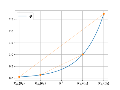
Figure 1: Graphical display of smooth ambiguity aversion at work. Although $\theta_{1}$ and $\theta_{2}$ yield the same loss $\mathcal{R}^{*}$ in $Q$-expectation, the ambiguity averse criterion favors the less variable decision $\theta_{1}$. Graphically, this is because the orange line connecting $\phi(\mathcal{R}_{p_{1}}(\theta_{1}))$ to $\phi(\mathcal{R}_{p_{2}}(\theta_{1}))$ lies (point-wise) below the line connecting $\phi(\mathcal{R}_{p_{1}}(\theta_{2}))$ to $\phi(\mathcal{R}_{p_{2}}(\theta_{2}))$.

Interestingly, Cerreia-Vioglio et al. (2011) showed that the SmAA model belongs to a general class of ambiguity-averse preferences, which admit a common utility function representation. For SmAA preferences with $\phi(t)=\beta\exp(\beta^{-1}t)-\beta$ (with $\beta>0$ and under additional technical assumptions), this representation implies the equivalence of problem (1) with

$$\min_{\theta\in\Theta}\max_{P:P\ll Q_{\bm{\xi}^{n}}}\big{\{}\mathbb{E}_{p\sim P}[\mathcal{R}_{p}(\theta)]-\beta\textnormal{KL}(P\|Q_{\bm{\xi}^{n}})\big{\}},$$

where $\textnormal{KL}(\cdot\|\cdot)$ is the Kullback-Leibler divergence and $\ll$ denotes absolute continuity. The above result further clarifies the mechanism through which distributional robustness is induced: Intuitively, instead of directly averaging over $p\sim Q_{\bm{\xi}^{n}}$, one computes a worst-case scenario w.r.t. the mixing measure, penalizing distributions that are further away from the posterior – the latter acts as a reference probability measure. Moreover, in the limiting case $\beta\to 0$, the mM-DRO setup is recovered, with ambiguity set

$$\mathcal{C}=\left\{p\in\mathscr{P}_{\Xi}:\exists P\ll Q_{\bm{\xi}^{n}},p=\int_{\mathscr{P}_{\Xi}}qP(\mathrm{d}q)\right\}.$$

In the other limiting case $\beta\to\infty$ (with the convention $0\cdot\infty=0$), the ambiguity neutral Bayesian criterion (2) is instead recovered.

3 Statistical Properties

In this section, we analyze the statistical properties of the criterion $V_{\bm{\xi}^{n}}(\theta)$, as a function of the sample size $n$. A first issue of interest, addressed in Proposition 2, is to study its asymptotic point-wise behavior.

Proposition 2.

Let $\bm{\xi}^{n}$ be iid according to $p_{*}$ and $\xi\mapsto h(\theta,\xi)$ continuous for all $\theta\in\Theta$. Then, for all $\theta\in\Theta$,

$$\lim_{n\to\infty}V_{\bm{\xi}^{n}}(\theta)=\phi(\mathcal{R}_{p_{*}}(\theta))$$

almost surely.

This ensures that, as more data are collected, the proposed criterion approaches, with probability 1, the true theoretical risk (up to the strictly increasing transformation $\phi$).

While point-wise convergence to the target ground truth is a first desirable property for any sensible criterion, it is not enough to characterize the behavior of the optimization’s out-of-sample performance, nor the closeness of the optimal criterion value and the criterion optimizer(s) to their theoretical counterparts. In the following subsections, we study these properties both in the finite-sample regime and in the asymptotic limit $n\to\infty$.

Finite-sample guarantees.

Denote

$$\theta_{n}\in\underset{\theta\in\Theta}{\arg\min}V_{\bm{\xi}^{n}}(\theta),\quad\theta_{*}\in\underset{\theta\in\Theta}{\arg\min}\mathcal{R}_{p_{*}}(\theta).$$

In finite-sample analysis, a first question of interest is whether probabilistic performance guarantees hold for the robust criterion optimizer $\theta_{n}$. In our setting, one can naturally measure performance by the narrowness of the gap between $\mathcal{R}_{p_{*}}(\theta_{n})$ and $\mathcal{R}_{p_{*}}(\theta_{*})$. As we clarify later, Lemma 3 is a first step towards establishing this type of guarantees.

Lemma 3.

Let $\phi$ be twice continuously differentiable on $(0,K)$, with $M_{\phi}:=\sup_{t\in(0,K)}\phi^{\prime}(t)$ and $\gamma_{\phi}(t):=\phi^{\prime\prime}(t)/\phi^{\prime}(t)\geq 0$. Then

$$\sup_{\theta\in\Theta}|V_{\bm{\xi}^{n}}(\theta) -\phi(\mathcal{R}_{p_{*}}(\theta))|$$

$$\leq M_{\phi}\Bigg{[}\frac{n}{\alpha+n}\sup_{\theta\in\Theta}|\mathcal{R}_{p_{\bm{\xi}^{n}}}(\theta)-\mathcal{R}_{p_{*}}(\theta)|\hskip 2.84544pt$$

$$+\hskip 2.84544pt\frac{\alpha}{\alpha+n}K\hskip 2.84544pt+\hskip 2.84544pt\frac{K^{2}}{2}\sup_{t\in(0,K)}\gamma_{\phi}(t)\Bigg{]}.$$

Lemma 3 links the $\sup$ distance of the criterion $V_{\bm{\xi}^{n}}$ from the theoretical risk to three key objects:

1. The classical $\sup$ distance between the empirical and theoretical risk, $\sup_{\theta\in\Theta}|\mathcal{R}_{p_{\bm{\xi}^{n}}}(\theta)-\mathcal{R}_{p_{*}}(\theta)|$;

2. The $\sup$ distance between the theoretical risk and the risk computed w.r.t. the base probability measure $p_{0}$, $\sup_{\theta\in\Theta}|\mathcal{R}_{p_{0}}(\theta)-\mathcal{R}_{p_{*}}(\theta)|$. This clarifies that, if $p_{0}$ is a good guess for $p_{*}$, i.e., if the above $\sup$ distance is small, adopting a Bayesian prior centered at $p_{0}$ can improve finite sample bounds;

3. The Arrow-Pratt coefficient $\gamma_{\phi}(t)$ of absolute ambiguity aversion. In the economic theory literature on decision-making under risk, this is a well-known concept measuring the degree of risk aversion of decision makers, with point-wise larger values of $\gamma_{\phi}$ corresponding to more risk aversion. See Klibanoff et al. (2005) for a discussion on the straightforward adaptation of this measure to the ambiguity (rather than risk) aversion setup we work in.

Most importantly, Lemma 3 allows us to prove the following Theorem, which yields the performance guarantees we are after.

Theorem 4.

For all $\delta>0$

$$\mathbb{P}[\mathcal{\phi}(\mathcal{R}_{p_{*}}(\theta_{n}))-\phi(\mathcal{R}_{p_{*}}(\theta_{*}))\leq\delta]$$

$$\geq\mathbb{P}\Bigg{[}\sup_{\theta\in\Theta}\left|\mathcal{R}_{p_{\bm{\xi}^{n}}}(\theta)-\mathcal{R}_{p_{*}}(\theta)\right|$$

$$\leq\hskip 2.84544pt\frac{\alpha+n}{n}\left(\frac{\delta}{2M_{\phi}}-\frac{\alpha}{\alpha+n}K-\frac{K^{2}}{2}\sup_{t\in(0,K)}\gamma_{\phi}(t)\right)\Bigg{]}.$$

Theorem 4 allows to obtain finite-sample probabilistic guarantees on the excess risk $\phi(\mathcal{R}_{p_{*}}(\theta_{n}))-\phi(\mathcal{R}_{p_{*}}(\theta_{*}))$ via bounds on $\sup_{\theta\in\Theta}\left|\mathcal{R}_{p_{\bm{\xi}^{n}}}(\theta)-\mathcal{R}_{p_{*}}(\theta)\right|$. The latter is a well-studied quantity, and the sought bounds follow from standard results relying on conditions on the complexity of the function class $\mathscr{H}:=\{h(\theta,\cdot):\theta\in\Theta\}$. We refer the reader to Wainwright (2019) for more details.

Asymptotic guarantees.

So far, we have studied the finite-sample behavior of the out-of-sample performance of $\theta_{n}$. Another closely related type of results deals with the asymptotic limit of such performance, as well as with the convergence of optimum criterion values and optimizing parameters to their ground-truth counterparts. In this Subsection, attention is turned to theoretical results of this kind.

Finite-sample guarantees on $\sup_{\theta\in\Theta}\left|\mathcal{R}_{p_{\bm{\xi}^{n}}}(\theta)-\mathcal{R}_{p_{*}}(\theta)\right|$ are usually of the form

$$\mathbb{P}\Big{[}\sup_{\theta\in\Theta}\left|\mathcal{R}_{p_{\bm{\xi}^{n}}}(\theta)-\mathcal{R}_{p_{*}}(\theta)\right|\leq\delta\Big{]}\geq 1-\eta_{n},$$

with $\sum_{n=1}^{\infty}\eta_{n}<\infty$. This implies (via a straightforward application of the first Borel-Cantelli Lemma) the almost sure vanishing of $\sup_{\theta\in\Theta}\left|\mathcal{R}_{p_{\bm{\xi}^{n}}}(\theta)-\mathcal{R}_{p_{*}}(\theta)\right|$. Thus, we include this as an assumption of the next Theorem. Moreover, we introduce a functional dependence of $\phi$ on $n$, and denote $\phi\equiv\phi_{n}$ accordingly.

Theorem 5.

Retain the assumptions of Lemma 3 and $\lim_{n\to\infty}\sup_{\theta\in\Theta}\left|\mathcal{R}_{p_{\bm{\xi}^{n}}}(\theta)-\mathcal{R}_{p_{*}}(\theta)\right|=0$ almost surely. Moreover, assume that $\phi_{n}$ satisfies:

1. $\lim_{n\rightarrow\noindent\infty}\sup_{t\in(0,K)}\gamma_{\phi_{n}}(t)=0$;

2. $\sup_{n\geq 1}M_{\phi_{n}}<\infty$;

3. $\lim_{n\rightarrow\infty}\sup_{t\in[0,K]}|\phi_{n}(t)-t|=0$.

Then the next two almost sure limits hold:

$$\lim_{n\rightarrow\infty}\mathcal{R}_{p_{*}}(\theta_{n})=\mathcal{R}_{p_{*}}(\theta_{*}),\quad\lim_{n\rightarrow\infty}V_{\bm{\xi}^{n}}(\theta_{n})=\mathcal{R}_{p_{*}}(\theta_{*}).$$

Theorem 5 is crucial because it ensures that, asymptotically, the excess risk vanishes and the finite-sample optimal value converges to the optimal value under the data generating process.

Remark 6.

From a design point of view, the type of $n$-dependent parametrization of $\phi$ required in Theorem 5 is sensible, as it is equivalent to adopting vanishing levels of ambiguity aversion (uniformly vanishing Arrow-Pratt coefficient) as the sample size grows – that is, as one obtains a more and more precise estimate of the true distribution $p_{*}$. Moreover, this assumption is in the spirit of the condition imposed on the radius of the Wasserstein ambiguity ball in Mohajerin Esfahani & Kuhn (2018), which is required to vanish as the sample size grows.

Remark 7.

Let $\phi(t)=\beta\exp(\beta^{-1}t)-\beta$ for some $\beta>0$. It is easy to see that $\phi$ is twice continuously differentiable, strictly increasing ($\phi^{\prime}(t)=\exp(\beta^{-1}t)>0$), strictly convex ($\phi^{\prime\prime}(t)=\beta^{-1}\exp(\beta^{-1}t)>0$) and has Arrow-Pratt coefficient $\gamma_{\phi}(t)=\beta^{-1}$. Moreover, restricting $\phi$ to the assumed domain $[0,K]$, one can show that, as $\beta\rightarrow\infty$, (i) $\phi$ converges uniformly to the identity map, (ii) $\phi^{\prime}$ converges uniformly to the constant function 1, and (iii) $\gamma_{\phi}$ converges uniformly to the constant function 0. That is, as $\beta\rightarrow\infty$, the ambiguity-neutral case is recovered. Thus, for the $n$-dependent choice of $\phi$, it is enough to choose $\phi_{n}(t)=\beta_{n}\exp(\beta_{n}^{-1}t)-\beta_{n}$ for some positive increasing sequence $(\beta_{n})_{n\geq 1}$ diverging to $\infty$. For the rest of the article, unless otherwise specified, we assume $\phi$ (or $\phi_{n}$) takes this exponential functional form.

Finally, we leverage the above results to ensure the convergence of the sequence of optimizers $(\theta_{n})_{n\geq 1}$ to a theoretical optimizer.

Theorem 8.

Let $\theta\mapsto h(\theta,\xi)$ be continuous for all $\xi\in\Xi$ and $\lim_{n\rightarrow\infty}\mathcal{R}_{p_{*}}(\theta_{n})=\mathcal{R}_{p_{*}}(\theta_{*})$ almost surely (e.g., as ensured in Theorem 5). Then, almost surely, $\lim_{n\to\infty}\theta_{n}=\bar{\theta}$ implies $\mathcal{R}_{p_{*}}(\bar{\theta})=\mathcal{R}_{p_{*}}(\theta_{*})$.

4 Monte Carlo Approximation

In what follows, we fix a sample $\bm{\xi}^{n}$ and propose simulation strategies to estimate $V_{\bm{\xi}^{n}}(\theta)$. The latter, in fact, is analytically intractable due to the infinite dimensionality of $Q_{\bm{\xi}^{n}}$. To that end, we exploit a key representation of DPs first established by Sethuraman (1994): If $p\sim\textnormal{DP}(\eta,q)$, then $p\overset{\textnormal{d}}{=}\sum_{j=1}^{\infty}p_{j}\xi_{j}$, where $\xi_{j}\overset{\textnormal{iid}}{\sim}q$ and the sequence of weights $(p_{j})_{j\geq 1}$ is constructed via a stick-breaking procedure based on iid $\textnormal{Beta}(1,\eta)$ samples (see Appendix B). Thus, for large enough integers $T$ and $N$, we propose the following Stick-Breaking Monte Carlo (SBMC) approximation for $V_{\bm{\xi}^{n}}(\theta)$:

$$\hat{V}_{\bm{\xi}^{n}}(\theta,T,N):=\frac{1}{N}\sum_{i=1}^{N}\phi\Bigg{(}\sum_{j=0}^{T}p_{ij}h(\theta,\xi_{ij})\Bigg{)},$$ (3)

where, $T$ denotes the number of stick-breaking steps performed before truncating each Monte Carlo sample from the DP posterior $Q_{\bm{\xi}^{n}}$, while $N$ denotes the number of such samples. Algorithm 1 details the procedure, which essentially approximates the posterior DP via truncation and takes expectations accordingly.

Algorithm 1 SBMC approximation

  Input: Data $\bm{\xi}^{n}$, model parameters, number of MC samples $N$, truncation step $T$

  for $i=1$ to $N$ do

     Set $\prod_{k=1}^{0}(1-B_{k})\equiv 1$

     for $j=1$ to $T$ do

        Draw $\xi_{ij}\sim\frac{\alpha}{\alpha+n}p_{0}+\frac{n}{\alpha+n}p_{\bm{\xi}^{n}}$

        Draw $B_{ij}\sim\textnormal{Beta}(1,\alpha+n)$

        Set $p_{ij}=B_{j}\prod_{k=1}^{j-1}(1-B_{k})$

     end for

     Draw $\xi_{i0}\sim\frac{\alpha}{\alpha+n}p_{0}+\frac{n}{\alpha+n}p_{\bm{\xi}^{n}}$

     Set $p_{i0}=\prod_{k=1}^{T}(1-B_{k})$

  end for

  Return: $N^{-1}\sum_{i=1}^{N}\phi\big{(}\sum_{j=0}^{T}p_{ij}h(\theta,\xi_{ij})\big{)}$

Remark 9.

We propose to truncate the stick-breaking procedure at some fixed step $T$. Another strategy would involve truncating it at a random step $T_{i}(\varepsilon):=\min\big{\{}t\in\mathbb{N}:\prod_{j=1}^{t}p_{ij}\leq\varepsilon\big{\}}$ for some small $\varepsilon>0$. This allows to directly control the approximation error at each Monte Carlo sample (Muliere & Tardella, 1998; Arbel et al., 2019), though it leads to simulated measures with supports of different cardinalities. For the sake of theory, we opt for the fixed-step/random-error approximation, though the random-step/fixed-error one is equally viable in practice.

Remark 10.

On top of being a theory-based approximation for $V_{\bm{\xi}^{n}}(\theta)$, the criterion (3) can be interpreted as implementing a form of robust Bayesian bootstrap. Instead of directly averaging the risk $h(\theta,\cdot)$ with respect to the empirical distribution, we first obtain $N$ bootstrap samples of size $T$ from the predictive (which is a compromise between the empirical and the prior centering distributions), we weight observations according to the stick-breaking procedure, and finally take a grand average of the $\phi$-transformed weighted sums. This connection with the Bayesian bootstrap suggests the following alternative Multinomial-Dirichlet Monte Carlo (MDMC) version of $V_{\bm{\xi}^{n}}(\theta)$:

$$\frac{1}{N}\sum_{i=1}^{N}\phi\Bigg{(}\sum_{j=1}^{T}w_{ij}h(\theta,\xi_{ij})\Bigg{)},$$

where $(w_{i1},\dots,w_{iT})\overset{\textnormal{iid}}{\sim}\textnormal{Dirichlet}\big{(}\alpha+n;\frac{\alpha+n}{T},\dots,\frac{\alpha+n}{T}\big{)}$ and the atoms are iid according to the predictive (see Algorithm 2 in Appendix B). For practical computation, we recommend using the MDMC approximation, as it tends to yield more balanced weights, compared to SBMC, even for low values of $T$.

With the following results, we ensure finite-sample and asymptotic guarantees on the closeness of optimization procedures based on the SBMC approximation versus the target $V_{\bm{\xi}^{n}}$.

Lemma 11.

Assume $\Theta$ is a bounded subset of $\mathbb{R}^{d}$ and, for all $\xi\in\Xi$, $\theta\mapsto h(\theta,\xi)$ is $c(\xi)$-Lipschitz continuous. Then, for all $T,N\geq 1$ and $\varepsilon>0$,

$$\sup_{\theta\in\Theta}\big{|}\hat{V}_{\bm{\xi}^{n}}(\theta,T,N) -V_{\bm{\xi}^{n}}(\theta)]\big{|}$$

$$\leq M_{\phi}K\Bigg{(}\frac{\alpha+n}{\alpha+n+1}\Bigg{)}^{T}+\varepsilon$$

with probability at least

$$1-2\left(\frac{32M_{\phi}C_{T}\textnormal{diam}(\Theta)\sqrt{d}}{\varepsilon}\right)^{d}$$

$$\times\left[\exp\left\{-\frac{3N\varepsilon^{2}}{4\phi(K)(6\phi(K)+\varepsilon)}\right\}+\exp\left\{-\frac{3N\varepsilon}{40\phi(K)}\right\}\right]$$

for some constant $C_{T}>0$.

Heuristically, the bound in Lemma 11 is obtained by decomposing the left-hand side of the inequality into a first term depending on the truncation error induced by the threshold $T$, and a second term reflecting the Monte Carlo error related to $N$. Moreover, analogously to Lemma 3, Lemma 11 easily implies finite-sample bounds on the excess “robust risk” $V_{\bm{\xi}^{n}}(\hat{\theta}_{n}(T,N))-V_{\bm{\xi}^{n}}(\theta_{n})$, where $\hat{\theta}_{n}(T,N)\in\arg\min_{\theta\in\Theta}\hat{V}_{\bm{\xi}^{n}}(\theta,T,N)$. Another consequence is the following asymptotic convergence Theorem, whose proof is analogous to that of Theorem 5.

Theorem 12.

Under the mild additional assumption that $\sup_{T\geq 1}C_{T}<\infty$ (see Appendix A for details on $C_{T}$),

$$\lim_{T,N\to\infty}\sup_{\theta\in\Theta}\big{|}\hat{V}_{\bm{\xi}^{n}}(\theta,T,N)-V_{\bm{\xi}^{n}}(\theta)]\big{|}=0$$

almost surely. Also,

$$\lim_{T,N\to\infty}\hat{V}_{\bm{\xi}^{n}}(\hat{\theta}_{n}(T,N),T,N) =V_{\bm{\xi}^{n}}(\theta_{n}),$$

$$\lim_{T,N\to\infty}V_{\bm{\xi}^{n}}(\hat{\theta}_{n}(T,N)) =V_{\bm{\xi}^{n}}(\theta_{n})$$

almost surely.

In words, Theorem 12 ensures that, as the truncation and MC approximation errors vanish, the optimal approximate criterion value converges to the optimal exact one, and that the exact criterion value at any approximate optimizer converges to the exact optimal value. Finally, as a byproduct of the above result, convergence of any approximate robust optimizer to an exact one is established as follows.

Theorem 13.

Let $\theta\mapsto h(\theta,\xi)$ be continuous for all $\xi\in\Xi$. Moreover, assume

$$\lim_{T,N\to\infty}V_{\bm{\xi}^{n}}(\hat{\theta}_{n}(T,N))=V_{\bm{\xi}^{n}}(\theta_{n})$$

almost surely (e.g., as ensured above). Then, almost surely, $\lim_{T,N\to\infty}\hat{\theta}_{n}(T,N)=\bar{\theta}_{n}$ implies $V_{\bm{\xi}^{n}}(\bar{\theta}_{n})=V_{\bm{\xi}^{n}}(\theta_{n})$.

5 Numerical Optimization and Experiments

In this Section, we apply our robust optimization procedure to a high-dimensional sparse linear regression task with simulated data. This is an especially fruitful setting to conduct experiments because: (i) The associated loss function (quadratic) is convex and differentiable almost everywhere, as for many other learning methods, so that any gradient-based optimization scheme and its associated convergence properties are easily transposed to those methods; (ii) we expect the high-dimensional and sparse nature of the problem to provide a good ground to test the robustness properties of our criterion, given the well-known performance limitations of standard least squares estimation in this context (Hastie et al., 2009); and (iii) due to the explainability of linear regression parameters, experimental results are easily interpreted and provide immediate insight into the workings of the proposed methodology. Appendix C presents one further experiment on Gaussian location parameter estimation in the presence of outliers, whose results are in line with those presented in this Section.

Gradient-based optimization.

Whether we resort to the SBMC or the MDMC approximation of $V_{\bm{\xi}^{n}}(\theta)$, we are faced with the task of minimizing a criterion of the form

$$V(\theta)=\frac{1}{N}\sum_{i=1}^{N}\phi\left(\sum_{j=1}^{T}p_{ij}h(\theta,\xi_{ij})\right).$$

The smoothness and convexity of $\phi$ make it appealing to minimize the criterion via gradient-based convex optimization techniques. Indeed, it is enough to assume that $\theta\mapsto h(\theta,\xi)$ is convex and differentiable (a standard assumption met in many applications of interest) to easily yield the same properties for $V$.

In light of this, assuming that $\theta\mapsto h(\theta,\xi)$ is differentiable at every $\xi_{ij}$ and denoting $H_{i}(\theta):=\sum_{j=1}^{T}p_{ij}h(\theta,\xi_{ij})$, the gradient of $V$ is

$$\nabla_{\theta}V(\theta) =\frac{1}{N}\sum_{i=1}^{N}\phi^{\prime}(H_{i}(\theta))\nabla_{\theta}H_{i}(\theta)$$ (4)

$$\equiv\frac{1}{M}\sum_{m=1}^{M}\ell_{m}\phi^{\prime}(H_{m}(\theta))\nabla_{\theta}h(\theta,\xi_{m}),$$

where $\ell_{m}\equiv Tp_{m}$ and the $m$-indexing is just a recoding of the indices (with a slight abuse of notation and $M\equiv N\cdot T$). That is, the gradient of $V(\theta)$ can be written as the average of $M$ terms. Thus, to minimize $V(\theta)$ we propose a mini-batch Stochastic Gradient Descent algorithm which, at each iteration $t$, updates the parameter vector as follows:

$$\theta^{t+1}=\theta^{t}-\eta_{t}\frac{1}{B}\sum_{m_{b}=1}^{B}\ell_{m_{b}}\phi^{\prime}(H_{m_{b}}(\theta^{t}))\nabla_{\theta}h(\theta^{t},\xi_{m_{b}}),$$ (5)

for a step-size $\eta_{t}>0$ and a random subset (mini-batch) of size $B$ from the indices $\{1,\dots,M\}$. Under standard regularity assumptions (Garrigos & Gower, 2023), in Proposition 19 (Appendix A) we prove convergence of the algorithm at usual rates for convex problems.

Remark 14.

Expression (C) provides some insight on how, in practice, distributional robustness is enforced. Notice that $H_{i}(\theta)=\mathcal{R}_{p_{i}}(\theta)$ is the expected risk computed according to $p_{i}$, an approximate realization from $Q_{\bm{\xi}^{n}}$. Thus, in the computation of the overall gradient $\nabla_{\theta}V(\theta)$, the gradients associated to the $p_{i}$’s that generate higher expected risks receive more weight (being $\phi$ convex, $\phi^{\prime}$ is increasing). These weights, then, are reflected into which gradients, in the mini-batch SGD algorithm, are given more leverage in updating the parameter vector. Thus, the procedure can be thought of as implementing a “soft worst-case scenario” scheme, whereby distributions in the posterior support are weighted (in terms of gradient influence) more the worse they do in terms of expected risk.

Experimental results.

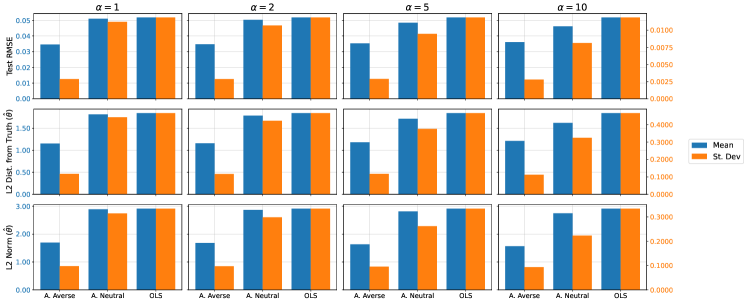
Figure 2: Simulation results for the high-dimensional sparse linear regression experiment. Bars report the mean and standard deviation (across 200 sample simulations) of the test RMSE, $L_{2}$ distance of estimated coefficient vector $\hat{\theta}$ from the data-generating one, and the $L_{2}$ norm of $\hat{\theta}$. Results are shown for the ambiguity-averse, ambiguity-neutral, and OLS procedures. Note: The left (blue) axis refers to mean values, the right (orange) axis to standard deviation values.

In our experiment, we simulate 200 independent samples of size 100 from a linear model with $d=90$ covariates $x_{1},\dots,x_{d}$, only the first $s=5$ of which have unitary positive marginal effect on the scalar response $y$. Moreover, all covariates have unitary variance and are moderately correlated with each other (see Appendix C for further details). Clearly, the model is high-dimensional ($d\approx n$) and sparse ($s\ll d$). It is reasonable to conjecture that these feature translate in high levels of uncertainty on the joint law of $(y,x_{1},\dots,x_{d})$, so that distributionally robust estimation may be beneficial in this setting. Therefore, we compare our ambiguity averse procedure (i.e., with $\phi$ chosen to be strictly convex) to the ambiguity neutral one ($\phi(t)=t$) and to standard Ordinary Least Squares (OLS) estimation. We choose the prior guess $p_{0}$ to be a $d+1$-dimensional standard normal distribution, which, as highlighted in Proposition 1, makes the ambiguity neutral procedure equivalent to $L_{2}$ (Ridge) regularization.

The results of our experiment, presented in Figure 2, provide insights into both average optimization outcomes and their sample variability, where especially the latter serves as a measure of robustness. In terms of out-of-sample performance, measured by the Root Mean Squared Error (RMSE) on a large test sample, our ambiguity-averse method surpasses OLS and the ambiguity-neutral criterion. Specifically, it exhibits lower average RMSE across various values of the concentration parameter $\alpha$ and demonstrates significantly reduced variability around the mean.

Furthermore, the ambiguity-averse criterion outperforms the other two methods in terms of parameter estimation accuracy. The $L_{2}$ distance between the estimated coefficient vector and the data-generating one is consistently lower on average and exhibits significantly less variability. This observation aligns with the capability of the ambiguity-averse procedure to more effectively shrink coefficients towards 0, as illustrated in the third row of Figure 2. In summary, our experimental results indicate that the smooth ambiguity-averse optimization procedure is effective in hedging against the distributional uncertainty inherent to the data-generating process, and suggests it as a promising approach for robust performance in challenging learning tasks.

6 Discussion

The paper tackled the problem of optimizing a data-driven criterion in the presence of distributional uncertainty about the data-generating mechanism. To mitigate the underperformance of classical methods, we introduced a novel distributionally robust criterion, drawing insights from Bayesian nonparametrics and a decision-theoretic model of smooth ambiguity aversion. We established connections with standard regularization techniques, including Ridge and LASSO regression, and theoretical analysis revealed favorable finite-sample and asymptotic guarantees on the performance of the robust procedure. For practical implementation, we presented and examined tractable approximations of the criterion, which are amenable to gradient-based optimization. Finally, we applied our method to a high-dimensional sparse linear regression task, offering insights into its practical robustness properties. Natural future directions arising from our work involve a deeper examination of the model workings in terms of (i) its parameter configuration and (ii) its broader application to general learning tasks. Additionally, our study offers prospects for investigating connections among such varied yet interconnected strands of literature as optimization, decision theory, and Bayesian statistics.

Supplement to “Bayesian Nonparametrics meets Data-Driven Robust Optimization”

This Supplement to “Bayesian Nonparametrics meets Data-Driven Robust Optimization” is organized as follows. In Appendix A, we collect the proofs of all results presented in the main text. In Appendix B, we provide further background on Dirichlet Process representations and related posterior simulation algorithms. Finally, in Appendix C, we describe in detail our simulation experiment.

Appendix A Technical proofs and further results

Proof of Proposition 2.

Let $\rightsquigarrow$ denote weak convergence of probability measures. By Corollary 4.17 in Ghosal & Van der Vaart (2017), $Q_{\bm{\xi}^{n}}\rightsquigarrow\delta_{p_{*}}$ almost surely. That is,

$$\lim_{n\rightarrow\infty}\int_{\mathscr{P}_{\Xi}}f(p)Q_{\bm{\xi}^{n}}(\mathrm{d}p)=f(p_{*})$$

almost surely for any bounded and continuous $f:\mathscr{P}_{\Xi}\rightarrow\mathbb{R}$. Thus, we are left to prove that $p\mapsto\phi(\mathcal{R}_{p}(\theta))$ is bounded and continuous for all $\theta\in\Theta$. It is bounded because $\phi$ is continuous on the compact interval $[0,K]$, and it is continuous because $p\mapsto\mathcal{R}_{p}(\theta)$ is continuous (by the definition of topology of weak convergence and because $\xi\mapsto h(\theta,\xi)$ is bounded and continuous) and $\phi$ is continuous.

Proof of Lemma 3.

First note that, by the stated assumptions, it follows from Taylor’s theorem that

$$\phi(\mathcal{R}_{p}(\theta))=\phi(\mathcal{R}_{p_{*}}(\theta))+\phi^{\prime}(\mathcal{R}_{p_{*}}(\theta))[\mathcal{R}_{p}-\mathcal{R}_{p_{*}}]+\frac{\phi^{\prime\prime}(c_{p,\theta})}{2}[\mathcal{R}_{p}-\mathcal{R}_{p_{*}}]^{2}$$

for all $p\in\mathscr{P}_{\Xi}$ and $\theta\in\Theta$ and for some $c_{p,\theta}\in[0,K]$. Then

$$\sup_{\theta\in\Theta}|V_{\bm{\xi}^{n}}(\theta)-\phi(\mathcal{R}_{p_{*}}(\theta))| =\sup_{\theta\in\Theta}\bigg{|}\phi^{\prime}(\mathcal{R}_{p_{*}}(\theta))\int_{\mathscr{P}_{\Xi}}\mathcal{[}\mathcal{R}_{p}-\mathcal{R}_{p_{*}}]Q_{\bm{\xi}^{n}}(\mathrm{d}p)$$

$$+\int_{\mathscr{P}_{\Xi}}\frac{\phi^{\prime\prime}(c_{p,\theta})}{2}[\mathcal{R}_{p}-\mathcal{R}_{p_{*}}]^{2}Q_{\bm{\xi}^{n}}(\mathrm{d}p)\bigg{|}$$

$$\leq M_{\phi}\sup_{\theta\in\Theta}\bigg{|}\frac{\alpha}{\alpha+n}\mathcal{R}_{p_{0}}(\theta)+\frac{n}{\alpha+n}\mathcal{R}_{p_{\bm{\xi}^{n}}}(\theta)-\mathcal{R}_{p_{*}}\bigg{|}$$

$$+M_{\phi}\sup_{\theta\in\Theta}\bigg{(}\int_{\mathscr{P}_{\Xi}}\frac{[\mathcal{R}_{p}(\theta)-\mathcal{R}_{p_{*}}(\theta)]^{2}}{2}Q_{\bm{\xi}^{n}}(\mathrm{d}p)\bigg{)}\sup_{t\in(0,K)}\gamma_{\phi}(t)$$

$$\leq M_{\phi}\Bigg{[}\frac{n}{\alpha+n}\sup_{\theta\in\Theta}|\mathcal{R}_{p_{\bm{\xi}^{n}}}(\theta)-\mathcal{R}_{p_{*}}(\theta)|+\frac{\alpha}{\alpha+n}K+\frac{K^{2}}{2}\sup_{t\in(0,K)}\gamma_{\phi}(t)\Bigg{]}.$$

Proof of Theorem 4.

Notice the following decomposition:

$$\underbrace{\mathcal{\phi}(\mathcal{R}_{p_{*}}(\theta_{n}))-\phi(\mathcal{R}_{p_{*}}(\theta_{*}))}_{\geq 0}$$ (6)

$$=\phi(\mathcal{R}_{p_{*}}(\theta_{n}))-V_{\bm{\xi}^{n}}(\theta_{n})+\underbrace{V_{\bm{\xi}^{n}}(\theta_{n})-V_{\bm{\xi}^{n}}(\theta_{*})}_{\leq 0}+V_{\bm{\xi}^{n}}(\theta_{*})-\phi(\mathcal{R}_{p_{*}}(\theta_{*}))$$

$$\leq 2\sup_{\theta\in\Theta}|V_{\bm{\xi}^{n}}(\theta)-\phi(\mathcal{R}_{p_{*}}(\theta))|.$$

Then, Lemma 3 implies that, for all $\delta>0$,

$$\mathbb{P}[\mathcal{\phi}(\mathcal{R}_{p_{*}}(\theta_{n}))-\phi(\mathcal{R}_{p_{*}}(\theta_{*}))\leq\delta]$$

$$\geq\mathbb{P}\left[\sup_{\theta\in\Theta}|V_{\bm{\xi}^{n}}(\theta)-\phi(\mathcal{R}_{p_{*}}(\theta))|\leq\delta/2\right]$$

$$\geq\mathbb{P}\left[M_{\phi}\Bigg{\{}\frac{n}{\alpha+n}\sup_{\theta\in\Theta}|\mathcal{R}_{p_{\bm{\xi}^{n}}}(\theta)-\mathcal{R}_{p_{*}}(\theta)|+\frac{\alpha}{\alpha+n}K+\frac{K^{2}}{2}\sup_{t\in(0,K)}\gamma_{\phi}(t)\Bigg{\}}\leq\delta/2\right]$$

$$=\mathbb{P}\left[\sup_{\theta\in\Theta}\left|\mathcal{R}_{p_{\bm{\xi}^{n}}}(\theta)-\mathcal{R}_{p_{*}}(\theta)\right|\hskip 2.84544pt\leq\hskip 2.84544pt\frac{\alpha+n}{n}\left(\frac{\delta}{2M_{\phi}}-\frac{\alpha}{\alpha+n}K-\frac{K^{2}}{2}\sup_{t\in(0,K)}\gamma_{\phi}(t)\right)\right].$$

Proof of Theorem 5.

Since

$$\lim_{n\rightarrow\infty}\sup_{\theta\in\Theta}|\mathcal{R}_{p_{\bm{\xi}^{n}}}(\theta)-\mathcal{R}_{p_{*}}(\theta)|=0$$

almost surely and given assumptions 1. and 2. on $\phi_{n}$, by Lemma 3 we obtain

$$\lim_{n\rightarrow\infty}\sup_{\theta\in\Theta}|V_{\bm{\xi}^{n}}(\theta)-\mathcal{\phi}_{n}(\mathcal{R}_{p_{*}}(\theta))|=0$$

almost surely. Then, by decomposition (6),

$$\lim_{n\rightarrow\infty}\phi_{n}(\mathcal{R}_{p_{*}}(\theta_{n}))-\phi_{n}(\mathcal{R}_{p_{*}}(\theta_{*}))=0$$

almost surely and

$$\lim_{n\rightarrow\infty}V_{\bm{\xi}^{n}}(\theta_{n})-V_{\bm{\xi}^{n}}(\theta_{*})=0$$

almost surely. As a consequence,

$$\lim_{n\rightarrow\infty}|V_{\bm{\xi}^{n}}(\theta_{n}) -\mathcal{\phi}_{n}(\mathcal{R}_{p_{*}}(\theta_{*}))|$$

$$\leq\lim_{n\rightarrow\infty}\left[|V_{\bm{\xi}^{n}}(\theta_{n})-V_{\bm{\xi}^{n}}(\theta_{*})|+|V_{\bm{\xi}^{n}}(\theta_{*})-\phi_{n}(\mathcal{R}_{p_{*}}(\theta_{*}))|\right]$$

$$\leq\lim_{n\rightarrow\infty}\left[|V_{\bm{\xi}^{n}}(\theta_{n})-V_{\bm{\xi}^{n}}(\theta_{*})|+\sup_{\theta\in\Theta}|V_{\bm{\xi}^{n}}(\theta)-\phi_{n}(\mathcal{R}_{p_{*}}(\theta))|\right]$$

$$=0$$

almost surely. Now recall assumption 3., i.e., the sequence $(\phi_{n})_{n\geq 1}$ converges uniformly to the identity map. Then, in light of the previous observations and by noticing that

$$|\mathcal{R}_{p_{*}}(\theta_{n})-\mathcal{R}_{p_{*}}(\theta_{*})| \leq|\mathcal{R}_{p_{*}}(\theta_{n})-\phi_{n}(\mathcal{R}_{p_{*}}(\theta_{n}))|+|\phi_{n}(\mathcal{R}_{p_{*}}(\theta_{n}))-\phi_{n}(\mathcal{R}_{p_{*}}(\theta_{*}))|$$

$$+|\phi_{n}(\mathcal{R}_{p_{*}}(\theta_{*}))-\mathcal{R}_{p_{*}}(\theta_{*})|$$

and

$$|V_{\bm{\xi}^{n}}(\theta_{n})-\mathcal{R}_{p_{*}}(\theta_{*})|\leq|V_{\bm{\xi}^{n}}(\theta_{n})-\phi_{n}(\mathcal{R}_{p_{*}}(\theta_{*}))|+|\phi_{n}(\mathcal{R}_{p_{*}}(\theta_{*}))-\mathcal{R}_{p_{*}}(\theta_{*})|,$$

the two desired almost sure limits follow:

$$\lim_{n\rightarrow\infty}\mathcal{R}_{p_{*}}(\theta_{n})=\mathcal{R}_{p_{*}}(\theta_{*}),\qquad\lim_{n\rightarrow\infty}V_{\bm{\xi}^{n}}(\theta_{n})=\mathcal{R}_{p_{*}}(\theta_{*}).$$

Proof of Theorem 8.

We have

$$\mathcal{R}_{p_{*}}(\theta_{*}) \leq\mathcal{R}_{p_{*}}(\bar{\theta})=\mathbb{E}_{\xi\sim p_{*}}\lim_{n^{\prime}\rightarrow\infty}h(\theta_{n},\xi)=\lim_{n\rightarrow\infty}\mathcal{R}_{p_{*}}(\theta_{n})=\mathcal{R}_{p_{*}}(\theta_{*})$$

almost surely, where the first equality follows from the continuity of $\theta\mapsto h(\theta,\xi)$ and the second one from the Dominated Convergence Theorem. Then, $\mathcal{R}_{p_{*}}(\bar{\theta})=\mathcal{R}_{p_{*}}(\theta_{*})$ almost surely, proving the result.

To Prove Lemma 11, we introduce two other Lemmas. After proving those, Lemma 11 follows immediately.

Lemma 15.

For all $T,N\geq 1$,

$$\sup_{\theta\in\Theta}|\hat{V}_{\bm{\xi}^{n}}(\theta,T,N)-V_{\bm{\xi}^{n}}(\theta)|\leq M_{\phi}K\Bigg{(}\frac{\alpha+n}{\alpha+n+1}\Bigg{)}^{T}+\sup_{\theta\in\Theta}\Big{|}\hat{V}_{\bm{\xi}^{n}}(\theta,T,N)-\mathbb{E}[\hat{V}_{\bm{\xi}^{n}}(\theta,T,1)]\Big{|}.$$ (7)

Proof.

We have

$$\sup_{\theta\in\Theta} |\hat{V}_{\bm{\xi}^{n}}(\theta,T,N)-V_{\bm{\xi}^{n}}(\theta)|$$

$$\leq\sup_{\theta\in\Theta}\Big{|}\hat{V}_{\bm{\xi}^{n}}(\theta,T,N)-\mathbb{E}[\hat{V}_{\bm{\xi}^{n}}(\theta,T,1)]\Big{|}+\sup_{\theta\in\Theta}\Big{|}\mathbb{E}[\hat{V}_{\bm{\xi}^{n}}(\theta,T,1)]-V_{\bm{\xi}^{n}}(\theta)\Big{|}.$$ (8)

Note that

$$\mathbb{E}[\hat{V}_{\bm{\xi}^{n}}(\theta,T,1)] =\mathbb{E}_{p_{1},\xi_{1},\dots,p_{T},\xi_{T}}\Bigg{[}\phi\Bigg{(}\sum_{j=1}^{T}p_{j}h(\theta,\xi_{j})+p_{0}h(\theta,\xi_{0})\Bigg{)}\Bigg{]}$$

$$=\mathbb{E}_{\sum_{j\geq 1}p_{j}\delta_{\xi_{j}}\sim Q_{\bm{\xi}^{n}}}\Bigg{[}\phi\Bigg{(}\sum_{j=1}^{T}p_{j}h(\theta,\xi_{j})+p_{0}h(\theta,\xi_{0})\Bigg{)}\Bigg{]}$$

$$=\mathbb{E}_{\sum_{j\geq 1}p_{j}\delta_{\xi_{j}}\sim Q_{\bm{\xi}^{n}}}\Bigg{[}\phi\Bigg{(}\sum_{j=1}^{\infty}p_{j}h(\theta,\xi_{j})+p_{0}h(\theta,\xi_{0})-\sum_{j=T+1}^{\infty}p_{j}h(\theta,\xi_{j})\Bigg{)}\Bigg{]}$$

$$=V_{\bm{\xi}^{n}}(\theta)+\mathbb{E}_{\sum_{j\geq 1}p_{j}\delta_{\xi_{j}}\sim Q_{\bm{\xi}^{n}}}\Bigg{[}\phi^{\prime}\big{(}c_{\theta,\sum_{j\geq 1}p_{j}\delta_{\xi_{j}}}\big{)}p_{0}\Bigg{\{}h(\theta,\xi_{0})-\sum_{j=T+1}^{\infty}\frac{p_{j}}{p_{0}}h(\theta,\xi_{j})\Bigg{\}}\Bigg{]},$$

where the last equality follows from the mean value theorem applied to endpoints $\sum_{j=1}^{\infty}p_{j}h(\theta,\xi_{j})$ and $\sum_{j=1}^{\infty}p_{j}h(\theta,\xi_{j})+p_{0}h(\theta,\xi_{0})-\sum_{j=T+1}^{\infty}p_{j}h(\theta,\xi_{j})$. Then the second term in (A) is bounded by

$$M_{\phi}K\mathbb{E}_{\sum_{j\geq 1}p_{j}\delta_{\xi_{j}}\sim Q_{\bm{\xi}^{n}}}[p_{0}]=M_{\phi}K\mathbb{E}\Bigg{[}\prod_{k=1}^{T}(1-B_{k})\Bigg{]}=M_{\phi}K\Bigg{(}\frac{\alpha+n}{\alpha+n+1}\Bigg{)}^{T}.$$

∎

The second term on the left-hand side of Equation(7) is instead of the form

$$\sup_{g\in\mathscr{G}}\bigg{|}\frac{1}{N}\sum_{i=1}^{N}g(X_{i})-\mathbb{E}[g(X_{1})]\bigg{|},$$ (9)

where $X_{i}=\sum_{j=0}^{T}p_{ij}h(\theta,\xi_{ij})$ are iid random variables whose distribution is determined by the truncated stick-breaking procedure.

The aim of the next Lemma is to provide sufficient conditions for finite sample bounds and asymptotic convergence to 0 of the term in (9). Specifically, we impose complexity constraints on the function class $\mathscr{H}:=\{\xi\mapsto h(\theta,\xi):\theta\in\Theta\}$ which allow us to obtain appropriate conditions on the derived class

$$\mathscr{F}:=\Bigg{\{}(p_{j},\xi_{j})_{j=0}^{T}\mapsto\phi\Bigg{(}\sum_{j=1}^{T}p_{j}h(\theta,\xi_{j})+p_{0}h(\theta,\xi_{0})\Bigg{)}:\theta\in\Theta\Bigg{\}},$$

ensuring the asymptotic and non-asymptotic results we seek.

Lemma 16.

Assume $\Theta$ is a bounded subset of $\mathbb{R}^{d}$ and $\theta\mapsto h(\theta,\xi)$ is $c(\xi)$-Lipschitz continuous for all $\xi\in\Xi$. Then, for all $T,N\geq 1$ and $\varepsilon>0$,

$$\sup_{\theta\in\Theta}\Big{|}\hat{V}_{\bm{\xi}^{n}}(\theta,T,N)-\mathbb{E}[\hat{V}_{\bm{\xi}^{n}}(\theta,T,1)]\Big{|}\leq\varepsilon$$

with probability at least

$$1-2\left(\frac{32M_{\phi}C_{T}\textnormal{diam}(\Theta)\sqrt{d}}{\varepsilon}\right)^{d}\left[\exp\left\{-\frac{3N\varepsilon^{2}}{4\phi(K)(6\phi(K)+\varepsilon)}\right\}+\exp\left\{-\frac{3N\varepsilon}{40\phi(K)}\right\}\right].$$

for some constant $C_{T}>0$.

Proof.

By the Lipschitz continuity assumption on $h(\theta,\xi)$, we obtain that, for all $(p_{j},\xi_{j})_{j=0}^{T}$, $\theta\mapsto\phi\left(\sum_{j=1}^{T}p_{j}h(\theta,\xi_{j})+p_{0}h(\theta,\xi_{0})\right)$ is $M_{\phi}\tilde{c}\big{(}(p_{j},\xi_{j})_{j=0}^{T}\big{)}$-Lipschitz continuous, with

$$\tilde{c}\big{(}(p_{j},\xi_{j})_{j=0}^{T}\big{)}:=\sum_{j=0}^{T}p_{j}c(\xi_{j}).$$

Indeed, for all $\theta_{1},\theta_{2}\in\Theta$,

$$\Bigg{|} \phi\Bigg{(}\sum_{j=1}^{T}p_{j}h(\theta_{1},\xi_{j})+p_{0}h(\theta_{1},\xi_{0})\Bigg{)}-\phi\Bigg{(}\sum_{j=1}^{T}p_{j}h(\theta_{2},\xi_{j})+p_{0}h(\theta_{2},\xi_{0})\Bigg{)}\Bigg{|}$$

$$\leq M_{\phi}\sum_{j=1}^{T}p_{j}|h(\theta_{1},\xi_{j})-h(\theta_{2},\xi_{j})|+p_{0}|h(\theta_{1},\xi_{0})-h(\theta_{2},\xi_{0})|$$

$$\leq M_{\phi}\tilde{c}\big{(}(p_{j},\xi_{j})_{j=0}^{T}\big{)}\|\theta_{1}-\theta_{2}\|.$$

Therefore, denoting by $P$ the law of the vector $(p_{j},\xi_{j})_{j=0}^{T}$ and by $N_{[]}(\varepsilon,\mathscr{F},\mathcal{L}^{1}(P))$ the associated $\varepsilon$-bracketing number of the class $\mathscr{F}$, by Lemma 7.88 in Lafferty et al. (2010) we obtain

$$N_{[]}(\varepsilon,\mathscr{F},\mathcal{L}^{1}(P))\leq\left(\frac{4M_{\phi}C\textnormal{diam}(\Theta)\sqrt{d}}{\varepsilon}\right)^{d},$$

with $C_{T}:=\int\tilde{c}\big{(}(p_{j},\xi_{j})_{j=0}^{T}\big{)}\mathrm{d}P$. Then the result follows by Theorem 7.86 in Lafferty et al. (2010) after noticing that $\sup_{f\in\mathscr{F}}\|f\|_{\mathcal{L}^{1}(P)}\leq\sup_{f\in\mathscr{F}}\|f\|_{\infty}\leq\phi(K)$. ∎

Proof of Theorem 13.

We have

$$V_{\bm{\xi}^{n}}(\theta_{n}) \leq V_{\bm{\xi}^{n}}(\bar{\theta}_{n})$$

$$=\mathbb{E}_{p\sim Q_{\bm{\xi}^{n}}}\left[\lim_{N\to\infty}\lim_{T\to\infty}\phi(\mathcal{R}_{p}(\hat{\theta}_{n}(T,N)))\right]$$

$$=\lim_{N\to\infty}\lim_{T\to\infty}V_{\bm{\xi}^{n}}(\hat{\theta}_{n}(T,N))$$

$$=V_{\bm{\xi}^{n}}(\theta_{n})$$

almost surely, where the first two equalities follow from the continuity of $\theta\mapsto h(\theta,\xi)$ and $\phi$ as well as from an iterated application of the Dominated Convergence Theorem (recall that $h(\theta,\xi)\in[0,K]$ by assumption for all $\theta$ and $\xi$). This implies $V_{\bm{\xi}^{n}}(\theta_{n})=V_{\bm{\xi}^{n}}(\bar{\theta}_{n})$ almost surely.

In the next result, we will assume $\phi(t)\equiv\phi_{\beta}(t)=\beta\exp(t/\beta)-\beta$. Moreover, we will emphasize, through superscripts, the dependence of mathematical objects on $\beta$ and the DP concentration parameter $\alpha$. Moreover, if necessary, we make the truncation threshold $T_{n}$ and the number of MC samples $N_{n}$ dependent on the sample size $n$.

Proposition 17.

Assume $\Theta$ is an open subset of $\mathbb{R}^{d}$ and $\lim_{N\to\infty}\lim_{T\to\infty}\sup_{\theta\in\Theta}|\hat{V}_{\bm{\xi}^{n}}^{\alpha,\beta}(\theta,T,N)-V_{\bm{\xi}^{n}}^{\alpha,\beta}(\theta)|=0$ almost surely for all $\alpha>0$ and $\beta>0$. Moreover, assume that

1. $\theta\mapsto h(\xi,\theta)$ is differentiable at $\theta_{*}\in\arg\min_{\theta\in\Theta}\mathcal{R}_{p_{*}}(\theta)$ for $p_{*}$-almost every $\xi\in\Xi$, with gradient $\nabla_{\theta_{*}}(\xi)$;

2. For all $\theta_{1}$ and $\theta_{2}$ in a neighborhood of $\theta_{*}$, there exists a measurable function $\xi\mapsto H(\xi)\in\mathcal{L}^{2}_{p_{*}}$ such that $|h(\theta_{1},\xi)-h(\theta_{2},\xi)|\leq H(\xi)\|\theta_{1}-\theta_{2}\|$;

3. $\theta\mapsto\mathcal{R}_{p_{*}}(\theta)$ admits a second-order Taylor expansion at $\theta_{*}$, with non-singular symmetric Hessian matrix $V_{\theta_{*}}$.

Then, with probability 1, there exist sequences $(T_{n})_{n\geq 1}$, $(N_{n})_{n\geq 1}$, $(\beta_{n})_{n\geq 1}$, (diverging to $\infty$) and $(\alpha_{n})_{n\geq 1}$ (converging to 0), such that

$$\sqrt{n}\big{(}\hat{\theta}_{n}^{\alpha_{n},\beta_{n}}(T_{n},N_{n})-\theta_{*}\big{)}\rightsquigarrow\mathcal{N}(0,V),\qquad V:=V_{\theta_{*}}^{-1}\mathbb{E}_{\xi\sim p_{*}}\big{[}\nabla_{\theta_{*}}(\xi)\nabla_{\theta_{*}}(\xi)^{\top}\big{]}V_{\theta_{*}}^{-1},$$

provided $\hat{\theta}_{n}^{\alpha_{n},\beta_{n}}(T_{n},N_{n})\overset{p}{\to}\theta_{*}$ as $n\to\infty$.

Proof.

The imposed assumptions match those listed in Theorem 5.23 of Van der Vaart (2000). The only condition left to prove is that there exist sequences $(T_{n})_{n\geq 1}$, $(N_{n})_{n\geq 1}$, $(\beta_{n})_{n\geq 1}$, (diverging to $\infty$) and $(\alpha_{n})_{n\geq 1}$ (converging to 0), such that $\mathcal{R}_{p_{\bm{\xi}^{n}}}(\hat{\theta}_{n}^{\alpha_{n},\beta_{n}}(T_{n},N_{n}))-\inf_{\theta\in\Theta}\mathcal{R}_{p_{\bm{\xi}^{n}}}(\theta)\leq o_{p}(n^{-1})$. We do so by proving that, for any fixed $n\geq 1$, $\mathcal{R}_{p_{\bm{\xi}^{n}}}(\hat{\theta}_{n}^{\alpha,\beta}(T,N))\to\inf_{\theta\in\Theta}\mathcal{R}_{p_{\bm{\xi}^{n}}}(\theta)$ almost surely as $\alpha\to 0$ and $\beta,T,N\to\infty$; this implies that, for all $n$, with probability 1 there exist $\alpha_{n},\beta_{n},T_{n}$ and $N_{n}$ such that $\mathcal{R}_{p_{\bm{\xi}^{n}}}(\hat{\theta}_{n}^{\alpha_{n},\beta_{n}}(T_{n},N_{n}))-\inf_{\theta\in\Theta}\mathcal{R}_{p_{\bm{\xi}^{n}}}(\theta)\leq\varepsilon_{n}$ for any $\varepsilon_{n}>0$. Moreover, it is easy to see that the result is implied by $\sup_{\theta\in\Theta}|\hat{V}^{\alpha,\beta}_{\bm{\xi}^{n}}(\theta,T,N)-\mathcal{R}_{p_{\bm{\xi}^{n}}}(\theta)|\to 0$, so we prove the latter. We have

$$\sup_{\theta\in\Theta} |\hat{V}^{\alpha,\beta}_{\bm{\xi}^{n}}(\theta,T,N)-\mathcal{R}_{p_{\bm{\xi}^{n}}}(\theta)|$$

$$\leq\sup_{\theta\in\Theta}|\hat{V}^{\alpha,\beta}_{\bm{\xi}^{n}}(\theta,T,N)-V^{\alpha,\beta}_{\bm{\xi}^{n}}(\theta)|+\sup_{\theta\in\Theta}|V^{\alpha,\beta}_{\bm{\xi}^{n}}(\theta)-\mathcal{R}_{p_{\bm{\xi}^{n}}}(\theta)|,$$

where the first term converges to 0 almost surely by assumption. Using a second-order Taylor expansion of $\phi_{\beta}(\mathcal{R}_{p}(\theta))$ around $\mathcal{R}_{p_{\bm{\xi}^{n}}}(\theta)$, the second term, instead, satisfies

$$\sup_{\theta\in\Theta} |V^{\alpha,\beta}_{\bm{\xi}^{n}}(\theta)-\mathcal{R}_{p_{\bm{\xi}^{n}}}(\theta)|=\sup_{\theta\in\Theta}\left|\int_{\mathscr{P}_{\Xi}}\phi_{\beta}(\mathcal{R}_{p}(\theta))Q^{\alpha}_{\bm{\xi}^{n}}(\mathrm{d}p)-\mathcal{R}_{p_{\bm{\xi}^{n}}}(\theta)\right|$$

$$\leq\sup_{\theta\in\Theta}\left|\phi^{\prime}_{\beta}(\mathcal{R}_{p_{\bm{\xi}^{n}}}(\theta))\left(\int_{\mathscr{P}_{\Xi}}\mathcal{R}_{p}(\theta)Q^{\alpha}_{\bm{\xi}^{n}}(\mathrm{d}p)-\mathcal{R}_{p_{\bm{\xi}^{n}}}(\theta)\right)\right|+\frac{K^{2}}{2}\sup_{t\in[0,K]}\phi_{\beta}^{\prime\prime}(t)$$

$$\leq\underbrace{\sup_{t\in[0,K]}\phi_{\beta}^{\prime}(t)}_{\to 1}\underbrace{\sup_{\theta\in\Theta}\left|\frac{n}{\alpha+n}\mathcal{R}_{p_{\bm{\xi}^{n}}}(\theta)+\frac{\alpha}{\alpha+n}\mathcal{R}_{p_{0}}(\theta)-\mathcal{R}_{p_{\bm{\xi}^{n}}}(\theta)\right|}_{\to 0}+\frac{K^{2}}{2}\underbrace{\sup_{t\in[0,K]}\phi_{\beta}^{\prime\prime}(t)}_{\to 0}\to 0,$$

as $\alpha\to 0$ and $\beta\to\infty$. ∎

Remark 18.

Theorems 8 and 13 ensure that (a) for all $n\geq 1$, provided $\hat{\theta}_{n}(T,N)$ converges almost surely to some $\theta_{n}\in\Theta$, the latter is a minimizer of $V_{\bm{\xi}^{n}}(\theta)$; and (b) if the above sequence $(\theta_{n})_{n\geq 1}$ converges almost surely to some $\theta_{*}\in\Theta$, the latter is a minimizer of $\mathcal{R}_{p_{*}}(\theta)$. Notice that the assumptions required for these results are consistent with the ones of Proposition 17, so they can be used to justify the condition $\hat{\theta}_{n}^{\alpha_{n},\beta_{n}}(T_{n},N_{n})\overset{p}{\to}\theta_{*}$. For instance, if one assumes almost sure uniqueness of minimizers and almost sure convergence of the above defined sequences, $\hat{\theta}_{n}^{\alpha_{n},\beta_{n}}(T_{n},N_{n})\overset{p}{\to}\theta_{*}$ can be guaranteed leveraging the preceding results.

Stochastic gradient descent convergence analysis.

For ease of exposition, we fix $B=1$ and denote by $\mathbb{E}_{t}$ the expectation operator conditional on the realization of the random index draws $m^{1},\dots,m^{t}\overset{\textnormal{iid}}{\sim}\textnormal{Uniform}(\{1,\dots,M\})$.

Proposition 19.

Assume that $V$ is convex and that $(\theta_{t})_{t\geq 1}$ follows Equation (5)) for some starting value $\theta^{0}\in\Theta$ and $B=1$. Moreover, assume that, for all $\theta\in\Theta$,

$$M^{-1}\sum_{m=1}^{M}\|\ell_{m}\phi^{\prime}(H_{m}(\theta))\nabla_{\theta}h(\theta,\xi_{m})\|^{2}\leq\sigma^{2}_{\nu}.$$

Then

$$\mathbb{E}_{T-1}[V(\tilde{\theta}^{T})]-V(\theta^{*})\leq\frac{\|\theta^{0}-\theta^{*}\|^{2}+\sigma^{2}_{\nu}\sum_{t=0}^{T}\eta_{t}^{2}}{2\sum_{t=0}^{T}\eta_{t}},$$

where $\theta^{*}\in\arg\min_{\theta\in\Theta}V(\theta)$, $\tilde{\theta}^{T}:=\sum_{t=0}^{T}\nu_{t}\theta^{t}$, and $\nu_{t}:=\frac{\eta_{t}}{\sum_{t^{\prime}=0}^{T}\eta_{t^{\prime}}}$.

Proof of Proposition 19.

Fix $t=1,\dots,T$. We have,

$$\|\theta^{t+1}-\theta^{*}\|^{2} =\|\theta^{t}-\eta_{t}\ell_{m^{t}}\phi^{\prime}(H_{m^{t}}(\theta^{t}))\nabla_{\theta}h(\theta^{t},\xi_{m^{t}})-\theta^{*}\|^{2}$$

$$=\|\theta^{t}-\theta^{*}\|^{2}+\eta_{t}^{2}\|\ell_{m^{t}}\phi^{\prime}(H_{m^{t}}(\theta^{t}))\nabla_{\theta}h(\theta^{t},\xi_{m^{t}})\|^{2}$$

$$-2\eta_{t}(\theta^{t}-\theta^{*})^{\top}\ell_{m^{t}}\phi^{\prime}(H_{m^{t}}(\theta^{t}))\nabla_{\theta}h(\theta^{t},\xi_{m^{t}}).$$

Applying the law of total expectation and the fact that $\ell_{m^{t}}\phi^{\prime}(H_{m^{t}}(\theta^{t}))\nabla_{\theta}h(\theta^{t},\xi_{m^{t}})$ is unbiased for $\nabla_{\theta}V(\theta^{t})$,

$$\mathbb{E}_{t}[(\theta^{t}-\theta^{*})^{\top}\ell_{m^{t}}\phi^{\prime}(H_{m^{t}}(\theta^{t}))\nabla_{\theta}h(\theta^{t},\xi_{m^{t}})] =\mathbb{E}_{t}[\mathbb{E}_{t-1}[(\theta^{t}-\theta^{*})^{\top}\ell_{m^{t}}\phi^{\prime}(H_{m^{t}}(\theta^{t}))\nabla_{\theta}h(\theta^{t},\xi_{m^{t}})]]$$

$$=\mathbb{E}_{t-1}[(\theta^{t}-\theta^{*})^{\top}\nabla_{\theta}V(\theta^{t})].$$

Hence

$$2\eta_{t}\mathbb{E}_{t-1}[(\theta^{t}-\theta^{*})^{\top}\nabla_{\theta}V(\theta^{t})] =\mathbb{E}_{t-1}[\|\theta^{t}-\theta^{*}\|^{2}]-\mathbb{E}_{t}[\|\theta^{t+1}-\theta^{*}\|^{2}]$$

$$+\eta_{t}^{2}\mathbb{E}_{t}[\|\ell_{m^{t}}\phi^{\prime}(H_{m^{t}}(\theta^{t}))\nabla_{\theta}h(\theta^{t},\xi_{m^{t}})\|^{2}]$$

$$\leq\mathbb{E}_{t-1}[\|\theta^{t}-\theta^{*}\|^{2}]-\underbrace{\mathbb{E}_{t}[\|\theta^{t+1}-\theta^{*}\|^{2}]}_{\geq 0}+\sigma^{2}_{\nu}.$$

Summing over $t=0,\dots,T$ and since

$$\mathbb{E}_{t-1}[(\theta^{t}-\theta^{*})^{\top}\nabla_{\theta}V(\theta^{t})]\geq\mathbb{E}_{t-1}[V(\theta^{t})-V(\theta^{*})]$$

because $V$ is convex, we have

$$2\sum_{t=0}^{T}\eta_{t}\mathbb{E}_{t-1}[V(\theta^{t})-V(\theta^{*})]\leq\|\theta^{0}-\theta^{*}\|^{2}+\sigma^{2}_{\nu}\sum_{t=0}^{T}\eta_{t}^{2}.$$

Dividing both sides by $\sum_{t=0}^{T}\eta_{t}$ and exploiting (i) the linearity of the expectation operator, (ii) the convexity of the weights $(\nu_{t})_{t=0}^{T}$, and (iii) the convexity of $V$, the result follows.

Proof of Proposition 1.

As for case 1, given the assumed form of $p_{0}$ and the criterion representation (2), we are left to establish an expression for $\mathbb{E}_{\xi\sim p_{0}}[h(\theta,\xi)]=\mathbb{E}_{(y,x)\sim\mathcal{N}(0,I)}[(y-\theta^{\top}x)^{2}]$. Notice that $-\theta_{j}x_{j}\overset{\textnormal{id}}{\sim}\mathcal{N}(0,\theta_{j}^{2})$, independendently of $y\sim\mathcal{N}(0,1)$, so that $y-\theta^{\top}x\sim\mathcal{N}(0,1+\|\theta\|_{2}^{2})$. Therefore, $\mathbb{E}_{\xi\sim p_{0}}[h(\theta,\xi)]=\mathbb{V}[y-\theta^{\top}x]=1+\|\theta\|_{2}^{2}$, which is easily seen to complete the proof. Finally, the proof for the LASSO case is completely analogous to the Ridge one and is therfore omitted.

Appendix B Further background on the Dirichlet Process and approximation algorithms

Since its definition by Ferguson (1973) based on the family of finite-dimensional Dirichlet distributions (as sketched in Section 2), the Dirichlet Process has been characterized (and thus generalized) in a number of useful ways. For instance, the DP can be derived as a neutral to the right process (Ferguson, 1974), a normalized completely random measure (Ferguson, 1973; Kingman, 1992; Lijoi & Prünster, 2010; Regazzini et al., 2003), a Gibbs-type prior (Gnedin & Pitman, 2006; De Blasi et al., 2015), a Pitman-Yor Process (Pitman, 1995; Perman et al., 1992), and a species sampling model (Pitman, 1996). In what follows, we review two other constructions of the DP which were at the basis of the approximate versions of the robust criterion $V_{\bm{\xi}^{n}}$ proposed in Section 4.

Stick-breaking construction of the Dirichlet Process.

Sethuraman (1994) proved that Ferguson’s (1973) Dirichlet Process enjoys the following “stick-breaking” representation

$$p\sim\textnormal{DP}(\alpha,P)\implies p\overset{\textnormal{d}}{=}\sum_{j=1}^{\infty}p_{j}\delta_{x_{j}},$$

where

$$x_{j} \overset{\textnormal{iid}}{\sim}P,\quad j=1,2,\dots,$$

$$p_{1} =B_{1},$$

$$p_{j} =B_{j}\prod_{i=1}^{j-1}B_{i},\quad j=2,3,\dots,$$

$$B_{j} \overset{\textnormal{iid}}{\sim}\textnormal{Beta}(1,\alpha),\quad j=1,2,\dots$$

The name of the procedure comes from the analogy with breaking a stick of length 1 into two pieces of length $B_{1}$ and $1-B_{1}$, then the second piece into two sub-pieces of length $(1-B_{1})B_{2}$ and $(1-B_{1})(1-B_{2})$, and so on. In Algorithm 1, then, we simulate $N$ realizations from $Q_{\bm{\xi}^{n}}$, truncating the stick-breaking procedure at step $j=T$. The remaining portion of the stick is then allocated to one further atom drawn from the predictive distribution. Then, the intractable integral with respect to the DP posterior is approximated via a Monte Carlo average of the integrals (i.e., weighted sums) with respect to the $N$ simulated measures.

Multinomial-Dirichlet construction of the Dirichlet Process and Monte Carlo Algorithms.

Another finite-dimensional approximation of $p\sim\textnormal{DP}(\alpha,P)$ is $p_{T}=\sum_{j=1}^{T}p_{j}\delta_{x_{j}}$, with $x_{j}\overset{\textnormal{iid}}{\sim}P$ and $(p_{1},\dots,p_{j})\sim\textnormal{Dirichlet}(T;\alpha/T,\dots,\alpha/T)$. As $T\to\infty$, $p_{T}$ approaches $p$ (see Theorem 4.19 in Ghosal & Van der Vaart, 2017). Hence, one can approximate $V_{\bm{\xi}^{n}}(\theta)$ as in Algorithm 2, where the concentration parameter is $\alpha+n$ and the centering distribution coincides with the predictive.

Algorithm 2 Multinomial-Dirichlet Monte Carlo (MDMC) approximation

  Input: Data $\bm{\xi}^{n}$, model parameters, number of MC samples $N$, approximation threshold $T$

  for $i=1$ to $N$ do

     Initialize $\bm{w}_{i}\in\mathbb{R}^{T},\bm{\xi}_{i}\in\Xi^{T}$

     for $j=1$ to $T$ do

        Update $\bm{w}_{i}(j)\sim\textnormal{Gamma}\big{(}\frac{\alpha+n}{T},1\big{)}$

        Update $\bm{\xi}_{i}(j)\sim\frac{\alpha}{\alpha+n}p_{0}+\frac{n}{\alpha+n}p_{\bm{\xi}^{n}}$

     end for

     Normalize $\bm{w}_{i}=\frac{\bm{w}_{i}}{\sum_{j=1}^{n}\bm{w}_{i}(j)}$

  end for

  Return: $N^{-1}\sum_{i=1}^{N}\phi\big{(}\bm{w}_{i}^{\top}h(\theta,\bm{\xi}_{i})\big{)}$

When $\alpha$ is negligible compared to the sample size $n$, one can simplify posterior simulation by setting $\alpha=0$. Thus, one obtains a $\textnormal{DP}(n,p_{\bm{\xi}^{n}})$ posterior. This distribution enjoys a useful representation as follows: $p\sim\textnormal{DP}(n,p_{\bm{\xi}^{n}})\implies p\overset{\textnormal{d}}{=}\sum_{i=1}^{n}p_{i}\xi_{i}$, with $p_{i}\sim\textnormal{Dirichlet}(n;1,\dots,1)$ (see Ghosal & Van der Vaart, 2017, Section 4.7). Due to its similarity to the usual bootstrap procedure (Efron, 1992), this distribution is known as the “Bayesian bootstrap”. Algorithm 3 implements the Bayesian bootstrap to approximate the criterion $V_{\bm{\xi}^{n}}(\theta)$. In practice, however, we do not recommend resorting to the Bayesian bootstrap approximation, since $\textnormal{DP}(n,p_{\bm{\xi}^{n}})$ assigns probability 1 to the set of distributions with strictly positive support on $\bm{\xi}^{n}$. This goes against the prescription that, as the finite sample $\bm{\xi}^{n}$ provides only partial information on the true underlying distribution, the statistical DM should be willing to consider a wider set of distributions other than the ones supported at the sample realizations.

Algorithm 3 Bayesian Bootstrap Monte Carlo (BBMC) approximation

  Input: Data $\bm{\xi}^{n}$, model parameters, number of MC samples $N$

  for $i=1$ to $N$ do

     Initialize $\bm{w}_{i}\in\mathbb{R}^{n}$

     for $j=1$ to $n$ do

        Update $\bm{w}_{i}(j)\sim\textnormal{Gamma}(1,1)$

     end for

     Normalize $\bm{w}_{i}=\frac{\bm{w}_{i}}{\sum_{j=1}^{n}\bm{w}_{i}(j)}$

  end for

  Return: $N^{-1}\sum_{i=1}^{N}\phi\big{(}\bm{w}_{i}^{\top}h(\theta,\bm{\xi}^{n})\big{)}$

Appendix C Experiment details

In this Section, we first describe the SGD algorithm used in practice for our experiments. Then, we describe in full detail the experiment on high-dimensional sparse linear regression. Finally, we present the details and results from the experiment on Gaussian location estimation with outliers.

Mini-batch stochastic gradient descent algorithm.

For practical optimization, we apply a modification to the SGD algorithm provided in Equation (5), which helps to reduce the computational burden of the procedure. Indeed, recall the formula of the gradient of the criterion $V$ that we need to optimize:

$$\nabla_{\theta}V(\theta) =\frac{1}{N}\sum_{i=1}^{N}\phi^{\prime}(H_{i}(\theta))\nabla_{\theta}H_{i}(\theta)$$

$$\equiv\frac{1}{M}\sum_{m=1}^{M}\ell_{m}\phi^{\prime}(H_{m}(\theta))\nabla_{\theta}h(\theta,\xi_{m}).$$

Clearly, then, implementing the baseline SGD algorithm requires, at each iteration, the evaluation of multiple $H_{m}(\theta^{t})$ terms, each consisting of $T$ evaluations of the loss function $h$. To avoid this, at each iteration we instead sub-sample one index $i=1,\dots,N$ and update the parameter vector according to the associated gradient $\phi^{\prime}(H_{i}(\theta^{t}))\nabla_{\theta}H_{i}(\theta^{t})$. The latter is still an unbiased estimator of the overall gradient of $V(\theta^{t})$, but it requires only $T$ evaluations of $h$ (plus those of $T$ gradients of $h$, similarly to the baseline algorithm). Finally, to exploit the whole data efficiently, we sub-sample without replacement and perform multiple passes over the $N$ MC samples. Algorithm 4 summarizes the procedure.

Algorithm 4 Modified Stochastic Gradient Descent algorithm

  Input: Approximate criterion parameters $\{(p_{ij},\xi_{ij}):i=1,\dots,N,j=1,\dots,T\}$, step size schedule $(\eta_{t})_{t\geq 0}$, starting value $\theta^{0}$, number of passes $P$, iteration tracker $t=0$

  for $p=1$ to $P$ do

     Initialize $I=\{1,\dots,N\}$

     for $j=1$ to $N$ do

        Sample uniformly $i\in I$

        Update $\theta^{t+1}=\theta^{t}-\eta_{t}\cdot\phi^{\prime}\big{(}\sum_{\ell=1}^{T}p_{i\ell}h(\theta^{t},\xi_{i\ell})\big{)}\cdot\sum_{\ell=1}^{T}p_{i\ell}\nabla_{\theta}h(\theta^{t},\xi_{i\ell})\big{)}$

        Update $I=I\setminus\{i\}$

        Update $t=t+1$

     end for

  end for

  Return: $\theta^{PN+1}$

C.1 Details on high-dimensional regression experiment

Data-generating process.

The data for the experiment are generated iid across simulations (200) and observations ($n=100$ per simulation) as follows. For each observation $i=1,\dots,n$, the $d$-dimensional ($d=90$) covariate vector follows a multivariate normal distribution with mean 0 and such that (i) each covariate has unitary variance, and (ii) any pair of distinct covariates has covariance 0.3:

$$x_{i}=\begin{bmatrix}x_{i1}\\ \vdots\\ x_{id}\end{bmatrix}\sim\mathcal{N}(0,\Sigma),\quad\Sigma=\begin{bmatrix}1&0.3&\cdots&0.3\\ 0.3&1&\cdots&0.3\\ \vdots&\vdots&\ddots&\vdots\\ 0.3&0.3&\cdots&1\end{bmatrix}\in\mathbb{R}^{d\times d}.$$

Then, the response has conditional distribution $y_{i}|x_{i}\sim\mathcal{N}(a^{\top}x_{i},\sigma^{2})$, with $a=(1,1,1,1,1,0,\cdots,0)^{\top}\in\mathbb{R}^{d}$ and $\sigma=0.5$. That is, out of 90 covariates, only the first 5 have a unitary positive marginal effect on $y_{i}$, and additive Gaussian noise is added to the resulting linear combination. Together with 100 training samples, at each simulation we generate 5000 test samples on which we compute out-of-sample RMSE for the ambiguity-averse, ambiguity-neutral, and OLS procedures.

Robust criterion parameters.

For each simulated sample, we run our robust procedure setting the following parameter values: $\phi(t)=\beta\exp(t/\beta)-\beta$, $\beta\in\{1,\infty\}$, $\alpha\in\{1,2,5,10\}$, and $p_{0}=\mathcal{N}(0,I)$, where the $\beta=\infty$ setting corresponds to Ridge regression with regularization parameter $\alpha/n$ (see Proposition 1). We use the quadratic loss function $(\theta,y,x)\mapsto 10^{-3}(y-\theta^{\top}x)^{2}$, where the $10^{-3}$ factor serves to stabilize numerical values in the optimization process. Notice that, by the form of the ambiguity-neutral criterion (2), the multiplicative factor on the loss function does not change the equivalence with Ridge. Finally, we run 300 Monte Carlo simulations to approximate the criterion, and truncate the Multinomial-Dirichlet approximation at $T=50$.

Stochastic gradient descent parameters

We initialize the algorithm at $\theta=(0,\dots,0)$ and set the step size at $\eta_{t}=50/(100+\sqrt{t})$. After visual inspection of convergence of the criterion value, we set the number of passes over data equal to 14.

C.2 Experiment on Gaussian location estimation with outliers

Setting.

In this experiment, we test the performance of our robust criterion on the task of estimating a univariate Gaussian mean (assuming the variance is known) when the data is corrupted by a few observations coming from a distant distribution. Clearly, this is a situation where a considerable level of distributional uncertainty is warranted. In this setting, the loss function $h(\xi,\theta)=(\xi-\theta)^{2}$ is simply the negative log-likelihood associated to the normal model. Notice that the $h$ is convex in $\theta$ and, as in the previous experiment, we pre-multiply it by a factor of $10^{-3}$ for numerical stability reasons.

Data-generating process.

The data for the experiment are generated iid across simulations (100) and observations ($n=13$ per simulation) as follows. For each simulation, 10 iid samples $x_{i}$ are drawn from a $\mathcal{N}(0,1)$ distribution (the actual data-generating process we want to learn) and 3 samples are drawn iid from a $\mathcal{N}(0,5)$ outlier distribution. At each simulation we also generate 5000 test samples from the data-generating process $\mathcal{N}(0,1)$, on which we compute the out-of-sample average negative log-likelihood for the ambiguity-averse, ambiguity-neutral, and Maximum Likelihood Estimation (MLE) procedures – this will be our measure of out of sample performance (see Figure 3).

Robust criterion parameters.

For each simulated sample, we run our robust procedure setting the following parameter values: $\phi(t)=\beta\exp(t/\beta)-\beta$, $\beta\in\{1,\infty\}$, $\alpha\in\{1,2,5,10\}$, and $p_{0}=\mathcal{N}(\mu_{0},I)$, where $\mu_{0}=(10\cdot 0+3\cdot 5)/(10+3)$ is a weighted average of the data-generating and the outlier means. By the expression of the ambiguity-neutral criterion (2), it is easy to show that the $\beta=\infty$ case leads to the parameter estimate

$$\hat{\theta}_{\bm{\xi}^{n}}=\frac{1}{\alpha+n}\sum_{i=1}^{\alpha+n}y_{i},$$

with $y_{i}=x_{i}$ for $i=1,\dots,n$ and $y_{i}=\mu_{0}$ for $i=n+1,\dots,n+\alpha$. That is, the ambiguity-neutral procedure with concentration parameter $\alpha\in\mathbb{N}$ is equivalent to the MLE procedure when the original training sample is enlarged with $\alpha$ additional observations equal to $\mu_{0}$. Finally, we run 300 Monte Carlo simulations to approximate the criterion, and truncate the Multinomial-Dirichlet approximation at $T=50$.

Stochastic gradient descent parameters.

We initialize the algorithm at $\theta=0$ and set the step size at $\eta_{t}=30/(100+\sqrt{t})$. After visual inspection of convergence of the criterion value, we set the number of passes over data equal to 27.

Results.

In Figure 3, we present the results of the simulation study. As for the regression experiment, the ambiguity-averse criterion brings improvement, across $\alpha$ values and compared to the ambiguity-neutral and the simple MLE procedures, both in terms of average performance and in terms of the latter’s variabiliy (see the first row of the Figure). From the second row of Figure 3, it also emerges that, on average, the ambiguity-averse procedure is more accurate at estimating the location parameter than the two other methods. Compared to the simple MLE procedure, the variability of the estimated parameter is also significantly smaller. Taken together, these results confirm the theoretical expectation that the ambiguity-averse optimization is effective at hedging against the distributional uncertainty arising in the estimation of corrupted data such as the simulated ones.

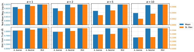
Figure 3: Simulation results from the experiment on Gaussian mean estimation with outliers. Bars report the mean and standard deviation (across 100 sample simulations) of the test mean log-likelihood and the absolute value distance of the estimated mean from 0 (the data-generating mean). Results are shown for the ambiguity-averse, ambiguity-neutral, and MLE procedures. Note: The left (blue) axis refers to mean values, the right (orange) axis to standard deviation values.

References

- Arbel et al. (2019) Arbel, J., De Blasi, P., and Prünster, I. Stochastic Approximations to the Pitman–Yor Process. Bayesian Analysis, 14(4):1201 – 1219, 2019.
- Ben-Tal et al. (2013) Ben-Tal, A., Den Hertog, D., De Waegenaere, A., Melenberg, B., and Rennen, G. Robust solutions of optimization problems affected by uncertain probabilities. Management Science, 59(2):341–357, 2013.
- Bertsimas et al. (2010) Bertsimas, D., Doan, X. V., Natarajan, K., and Teo, C.-P. Models for minimax stochastic linear optimization problems with risk aversion. Mathematics of Operations Research, 35(3):580–602, 2010.
- Blackwell & MacQueen (1973) Blackwell, D. and MacQueen, J. B. Ferguson distributions via Pólya urn schemes. The Annals of Statistics, 1(2):353–355, 1973.
- Cerreia-Vioglio et al. (2011) Cerreia-Vioglio, S., Maccheroni, F., Marinacci, M., and Montrucchio, L. Uncertainty averse preferences. Journal of Economic Theory, 146(4):1275–1330, 2011.
- Cerreia-Vioglio et al. (2013) Cerreia-Vioglio, S., Maccheroni, F., Marinacci, M., and Montrucchio, L. Ambiguity and robust statistics. Journal of Economic Theory, 148(3):974–1049, 2013.
- Christensen (2020) Christensen, R. Plane Answers to Complex Questions: The Theory of Linear Models. Springer, 2020.
- De Blasi et al. (2015) De Blasi, P., Favaro, S., Lijoi, A., Mena, R. H., Prünster, I., and Ruggiero, M. Are gibbs-type priors the most natural generalization of the dirichlet process? IEEE transactions on pattern analysis and machine intelligence, 37(2):212–229, 2015.
- Delage & Ye (2010) Delage, E. and Ye, Y. Distributionally robust optimization under moment uncertainty with application to data-driven problems. Operations research, 58(3):595–612, 2010.
- Duchi & Namkoong (2021) Duchi, J. C. and Namkoong, H. Learning models with uniform performance via distributionally robust optimization. The Annals of Statistics, 49(3):1378–1406, 2021.
- Efron (1992) Efron, B. Bootstrap methods: another look at the jackknife. In Breakthroughs in statistics: Methodology and distribution, pp. 569–593. Springer, 1992.
- Ferguson (1973) Ferguson, T. S. A Bayesian analysis of some nonparametric problems. The Annals of Statistics, pp. 209–230, 1973.
- Ferguson (1974) Ferguson, T. S. Prior distributions on spaces of probability measures. The Annals of Statistics, 2(4):615–629, 1974.
- Garrigos & Gower (2023) Garrigos, G. and Gower, R. M. Handbook of convergence theorems for (stochastic) gradient methods. arXiv preprint arXiv:2301.11235, 2023.
- Ghosal & Van der Vaart (2017) Ghosal, S. and Van der Vaart, A. Fundamentals of nonparametric Bayesian inference, volume 44. Cambridge University Press, 2017.
- Gilboa & Marinacci (2016) Gilboa, I. and Marinacci, M. Ambiguity and the Bayesian paradigm. Readings in formal epistemology: Sourcebook, pp. 385–439, 2016.
- Gilboa & Schmeidler (1989) Gilboa, I. and Schmeidler, D. Maxmin expected utility with non-unique prior. Journal of mathematical economics, 18(2):141–153, 1989.
- Gnedin & Pitman (2006) Gnedin, A. and Pitman, J. Exchangeable gibbs partitions and stirling triangles. Journal of Mathematical Sciences, 138(3):5674–5685, 2006.
- Hastie et al. (2009) Hastie, T., Tibshirani, R., and Friedman, J. The elements of statistical learning: Data mining, inference, and prediction, 2009.
- Hoerl & Kennard (1970) Hoerl, A. E. and Kennard, R. W. Ridge regression: Biased estimation for nonorthogonal problems. Technometrics, 12(1):55–67, 1970.
- Kingman (1992) Kingman, J. F. C. Poisson processes, volume 3. Clarendon Press, 1992.
- Klibanoff et al. (2005) Klibanoff, P., Marinacci, M., and Mukerji, S. A smooth model of decision making under ambiguity. Econometrica, 73(6):1849–1892, 2005.
- Kuhn et al. (2019) Kuhn, D., Esfahani, P. M., Nguyen, V. A., and Shafieezadeh-Abadeh, S. Wasserstein distributionally robust optimization: Theory and applications in machine learning. In Operations research & management science in the age of analytics, pp. 130–166. INFORMS, 2019.
- Lafferty et al. (2010) Lafferty, J., Liu, H., and Wasserman, L. Concentration of measure. Technical report, Carnegie Mellon University, 2010. URL https://www.stat.cmu.edu/~larry/=sml/Concentration.pdf.
- Lijoi & Prünster (2010) Lijoi, A. and Prünster, I. Models beyond the Dirichlet process. In Hjort, N. L., Holmes, C., Müller, P., and Walker, S. G. (eds.), Bayesian Nonparametrics, Cambridge Series in Statistical and Probabilistic Mathematics, pp. 80–136. Cambridge University Press, 2010.
- Lyddon et al. (2018) Lyddon, S., Walker, S., and Holmes, C. C. Nonparametric learning from Bayesian models with randomized objective functions. Advances in Neural Information Processing Systems, 31, 2018.
- Majumdar (1992) Majumdar, S. On topological support of Dirichlet prior. Statistics & Probability Letters, 15(5):385–388, 1992.
- Mohajerin Esfahani & Kuhn (2018) Mohajerin Esfahani, P. and Kuhn, D. Data-driven distributionally robust optimization using the Wasserstein metric: Performance guarantees and tractable reformulations. Mathematical Programming, 171(1-2):115–166, 2018.
- Muliere & Tardella (1998) Muliere, P. and Tardella, L. Approximating distributions of random functionals of Ferguson-Dirichlet priors. Canadian Journal of Statistics, 26(2):283–297, 1998.
- Perman et al. (1992) Perman, M., Pitman, J., and Yor, M. Size-biased sampling of poisson point processes and excursions. Probability Theory and Related Fields, 92(1):21–39, 1992.
- Pitman (1995) Pitman, J. Exchangeable and partially exchangeable random partitions. Probability theory and related fields, 102(2):145–158, 1995.
- Pitman (1996) Pitman, J. Some developments of the Blackwell-Macqueen urn scheme. In Ferguson, T. S., Shapley, L. S., and MacQueen, J. B. (eds.), Statistics, probability and game theory: Papers in honor of David Blackwell, volume 30 of IMS Lecture Notes - Monograph Series, pp. 245–267. Institute of Mathematical Statistics, 1996.
- Rahimian & Mehrotra (2022) Rahimian, H. and Mehrotra, S. Frameworks and results in distributionally robust optimization. Open Journal of Mathematical Optimization, 3:1–85, 2022.
- Regazzini et al. (2003) Regazzini, E., Lijoi, A., and Prünster, I. Distributional results for means of normalized random measures with independent increments. The Annals of Statistics, 31(2):560–585, 2003.
- Savage (1972) Savage, L. J. The foundations of statistics. Courier Corporation, 1972.
- Seber & Lee (2003) Seber, G. A. and Lee, A. J. Linear regression analysis. John Wiley & Sons, 2003.
- Sethuraman (1994) Sethuraman, J. A constructive definition of Dirichlet priors. Statistica sinica, pp. 639–650, 1994.
- Tibshirani (1996) Tibshirani, R. Regression shrinkage and selection via the lasso. Journal of the Royal Statistical Society Series B: Statistical Methodology, 58(1):267–288, 1996.
- Van der Vaart (2000) Van der Vaart, A. W. Asymptotic statistics, volume 3. Cambridge university press, 2000.
- Wainwright (2019) Wainwright, M. J. High-dimensional statistics: A non-asymptotic viewpoint, volume 48. Cambridge University Press, 2019.
- Wang et al. (2022) Wang, S., Wang, H., and Honorio, J. Distributional robustness bounds generalization errors. arXiv preprint arXiv:2212.09962, 2022.
- Wiesemann et al. (2013) Wiesemann, W., Kuhn, D., and Rustem, B. Robust Markov decision processes. Mathematics of Operations Research, 38(1):153–183, 2013.