WetSpongeCake: a Surface Appearance Model Considering Porosity and Saturation

Abstract.

Wet powdered materials, like wet ground or moist walls, widely exist in the real world. In these materials, the individual powder or particle is invisible at the macroscopic view, although its size is larger than the wavelength. Faithfully reproducing these appearances is vital in many applications. Existing approaches characterize these effects in different ways. An accurate way is to perform Monte Carlo path tracing on implicit shapes (e.g., sphere or ellipsoid), leading to expensive time costs despite their accuracy. The second kind of works model the powdered materials with a medium using the original or modified radiative transfer equation. However, these methods have extensive computational costs, preventing them from practical use, and also lack controllable intuitive physical parameters. The other line of works represent porosity effects with cylinder-shaped holes on surfaces. Despite their time efficiency, they do not allow transmission and can not closely match real-world effects. In this paper, we propose a new practical bidirectional scattering distribution function (BSDF) model– WetSpongeCake, with controllable physical parameters for wet powdered materials, which can reproduce real-world appearances faithfully and remains practical as well. To this end, we first reformulate the Monte Carlo light transport on implicit shapes into a medium, where at the core is an equivalent phase function as an aggregation for the light transport within ellipsoid-shaped particles, together with a modified RTE to enable porosity and saturation effects. Then, we propose our novel surface BSDF WetSpongeCake by integrating our proposed medium into the SpongeCake framework. As a result, our WetSpongeCake model is able to represent various appearances of wet powdered materials using physical parameters (e.g., porosity and saturation), allowing both reflection and transmission. We demonstrate our model on several examples: a piece of wet paper, sand saturated with different liquids, or sculptures made of multiple particles.

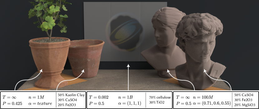
Figure 1. In this paper, we present a surface appearance model –WetSpongeCake, to represent wet powdered materials with physical parameters. It can produce vivid appearances on a wide range of materials. Examples include the wet paper, flowerpots and sculptures as shown above.

1. Introduction

Reproducing appearances from the real world with material models is essential in computer graphics. Material models for some common appearances (e.g., plastic, metals, glasses, etc.) have been extensively developed with surface shading models (e.g., microfacet models (Cook and Torrance, 1982; Walter et al., 2007)). Unfortunately, these widely-used shading models have limited capability to represent wet powdered materials. Examples of this kind of materials include a damp road or wet sand (see Fig. 2). Generally, the powdered materials are made of discrete powders, where the particle size is larger than the wavelength. After filling the materials with some liquids, they become wet. These appearances have become crucial for many applications, like wet roads in the autonomous driving simulation. However, it’s challenging to simulate these materials, as it involves complex optical phenomena.

Existing approaches simulate these effects in different ways. The most accurate ones treat individual powder particle as a sphere (Peltoniemi and Lumme, 1992) or an ellipsoid (Kimmel and Baranoski, 2007) and then perform Monte Carlo simulation on a set of particles. Despite their accuracy and physical parameters, these methods are computationally expensive, preventing them from practical use. Another group of methods model the powdered materials with a medium, by the original radiative transfer equation (RTE) (Jensen et al., 1999) or modified RTE (Hapke, 2008, 1999; Shkuratov et al., 1999) for non-continuous media with a porosity parameter. However, these methods lack controllable physical parameters and are still too time-consuming for practical use due to the random walk within the medium. The last line of works model powdered materials as a bidirectional reflectance distribution function (BRDF) (Merillou et al., 2000; Hnat et al., 2006; Lu et al., 2006), introducing cylinder-shaped holes on the surface. Although these approaches are practical, they have limited capability to match the real-world effects and can not simulate the transmission effects. For example, an interesting observation is that a minor difference in the refraction index of liquids leads to a significant difference in darkness (see Fig. 9), which can not be reproduced by the above surface models.

In this paper, we propose a new bidirectional scattering distribution function (BSDF) model with controllable physical parameters for wet powdered materials, which can closely match the real-world effect and remain practical. To this end, we first reformulate the Monte Carlo light transport on shapes into a medium, where at the core is an equivalent phase function to approximate the light transport within ellipsoid particles, together with a modified RTE to enable saturation effects. Then, we propose our novel surface BSDF WetSpongeCake by integrating the proposed medium into the SpongeCake framework, using the position-free theory, where the single scattering can be computed analytically, and the multiple scattering relies on the position-free Monte Carlo simulation. Our WetSpongeCake model can faithfully reproduce wet powdered materials with physical parameters (e.g., porosity, saturation, etc.). It is capable of representing a wide range of appearances. We demonstrate our model on several examples: a piece of wet paper, saturated sand, or sculptures. To summarize, our contributions include:

• a new practical surface model WetSpongeCake to represent wet powdered materials with physical parameters,

• an equivalent phase function to aggregate the complex light transport within a particle, which can match the references closely, and

• a modified radiative transfer equation to model both porosity and saturation.

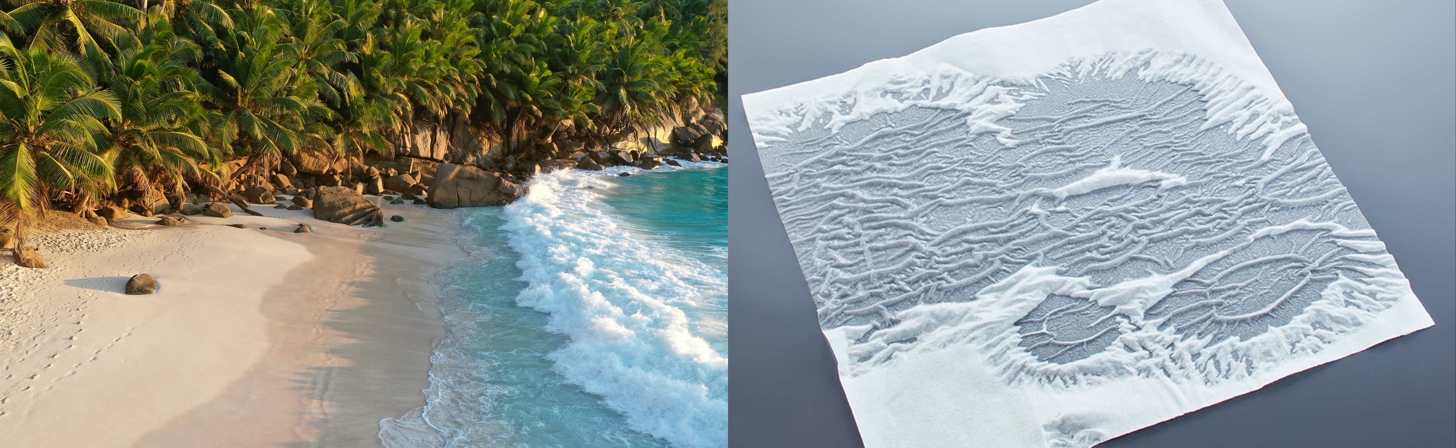
Figure 2. The appearances of wet powdered materials in the real world. Left: Photo by Chris on Unsplash; Right: Photo by BananaHub on Shutterstock

2. Related Work

2.1. Wet material models

Several ways have been proposed to represent wet materials in the literature, which can be grouped into three types: Monte Carlo rendering models on particle shapes, medium-based models, and surface-based BRDFs.

In the first group, two typical methods treat individual powder particle as a sphere (Peltoniemi and Lumme, 1992) or an ellipsoid (Kimmel and Baranoski, 2007) and then perform Monte Carlo simulation on a set of particles. These methods can achieve high-fidelity renderings, but are too computationally expensive. Similar to Kimmel et al. (2007), we also model each particle with an ellipsoid and have similar physical parameters as their model. However, we simplify the light transport within a particle with a fitted phase function and derive a lightweight BSDF rather than a random walk among the particles.

Jensen et al. (1999) capture the wetness of materials with a combined surface and subsurface model, leveraging a two-term Henyey-Greenstein (HG) phase function to approximate the scattering of particles. Their method provides convincing results. However, as their method lacks physical-meaning parameters, they tweak the HG parameter manually for control. Also, it has been pointed out that the powdered materials can not be represented by continuous RTE by several works (Hapke, 2008, 1999; Shkuratov et al., 1999). Instead, these works replace the original RTE with modified ones by including a porosity parameter. Despite their ability to represent porosity, they can not handle wet materials. All these medium-based approaches need volumetric path tracing, leading to numerous time costs. Several methods (Moon et al., 2007; Meng et al., 2015; Müller et al., 2016) have been proposed for simulating the light transport for visible discrete particles, which are out of our scope.

Several works represent the wet materials with surface models, including Lekner and Dorf (1988) and Bajo et al. (2021), where the former is based on Angstrom’s model (1925), and the latter further improves the model by Lekner et al. (1988). The other real-time surface models (Hnat et al., 2006; Merillou et al., 2000; Lu et al., 2006) introduce a cylinder-like shape for holes and apply intrinsic roughness on the hole surfaces. These approaches are lightweight and practical. However, these methods have difficulty matching the real-world effects closely. As pointed out by Twomey et al. (1986), when applying different liquids to the powdered materials, a minor refractive index difference (water and benzene on the wet sand (Bohren, 1983)) can lead to significantly different appearances, which is unable to be modeled by surface models, due to its small extinction. Compared to these empirical surface models, our method is physically based and can closely match real-world phenomena.

2.2. Position-free BSDFs

The position-free property has been introduced into surface models by Guo et al. (2018). The key idea of this property is to reformulate path integral within a medium from the entire spatial dimensions to the depth dimension only, as the incident and exit rays share the same position. This simplification of the path integral leads to a more efficient BSDF evaluation. This idea has been used further by Xia et al. (2020) and Gamboa et al. (2020) for more advanced sampling approaches, or modeling pearlescent pigments (Guillén et al., 2020). Recently, the SpongeCake model by Wang et al. (Wang et al., 2022b) further improves their efficiency by assuming volume-only slabs without any surface interfaces, leading to the analytical single scattering formulation. Furthermore, their multiple scattering is approximated by the single scattering with modified parameters, leading to noise-free BSDF evaluation.

We also apply this position-free idea to our method by integrating the medium into the SpongeCake framework. Regarding the multiple scattering, we keep the Monte Carlo estimator for simplification, similar to Guo et al. (2018). Using the multiple scattering solution in the SpongeCake model will further improve efficiency, and we leave it for future work.

2.3. Microfacet models

The microfacet models (Cook and Torrance, 1982; Walter et al., 2007) have been widely used to represent common materials in the real world. There are numerous works on the microfacet models for multiple scattering computations under the Smith assumption (Heitz et al., 2016; Bitterli and d’Eon, 2022; Wang et al., 2022a; Cui et al., 2023) or with the V-groove profile (Lee et al., 2018; Xie and Hanrahan, 2018), normal distribution function  (Beckmann and Spizzichino, 1963; Walter et al., 2007), and importance sampling (Heitz and d’Eon, 2014). The other works aim at higher expressing ability (Burley and Studios, 2012; Lucas et al., 2023) or practical use (Kulla and Conty, 2017; Turquin, 2019).

Compared to the above methods, our BSDF has introduced more parameters, including porosity and saturation, besides the material roughness, enabling a more prosperous representation of materials.

Table 1. Notations.

Mathematical notation
$\Omega$	full spherical domain
$\cos{\mathbf{\omega}}$	The cosine of the angle between ${\mathbf{\omega}}$ and the z-axis
${\mathbf{\omega}}_{i}\cdot{\mathbf{\omega}}_{o}$	dot product
Physical quantities
$\omega_{i}$	incident direction
$\omega_{o}$	outgoing direction
$f_{p}(\theta)$	phase function
Phase function parameters
$\eta_{p}$	refractive index of particle
$\eta_{l}$	refractive index of liquid
$\Psi$	sphericity
$R$	roundness
$\alpha$	albedo
Medium parameters
$T$	thickness
$S$	saturation
$P$	porosity
$n$	particle count per unit volume
${\sigma_{t}^{l}}$	liquid extinction coefficient

3. Preliminaries

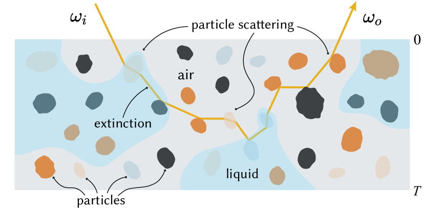
Figure 3. Wet powdered material is made of discrete particles (maybe multiple types), air, and liquid, where each particle has a rough surface described by the microfacet model, and the liquid may have absorption. After a light ray enters this material, it can be either reflected or refracted by the particle surface and travels in the air or the liquid. The ray is bounced within this material until it leaves the surface.

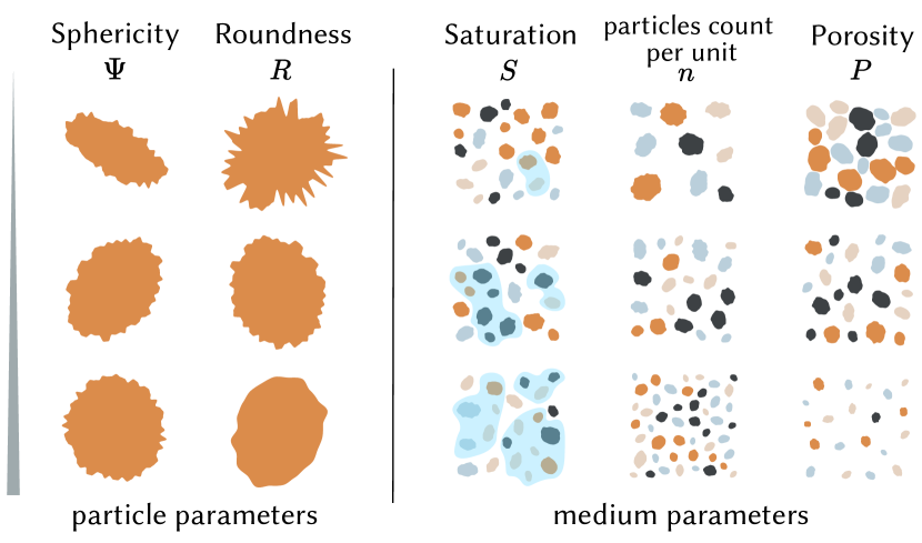
Figure 4. Several examples of parameters defined on particles and medium.

In this paper, we aim at simulating wet powdered materials. Among the existing approaches for this kind of materials, the ones that model particles as shapes (e.g., ellipsoid (Kimmel and Baranoski, 2007)) and use Monte Carlo path tracing have the highest fidelity. Therefore, we first introduce such a full formulation in this section and then propose our solution as a practical approximation in the following sections.

As shown in Fig. 3, the wet powdered materials consist of millions of particles with the air and liquid in between, forming a volume. As for each particle, we model its shape as an ellipsoid with parameters sphericity $\Psi$ and its appearance with several parameters, including the refractive index $\eta_{p}$, roughness $R$, and albedo $\alpha$ under the microfacet model, similar to Kimmel et al. (2007). There may be one type or multiple types of particles, and the particle count per unit volume is denoted by $n$. The porosity is the fraction of the volume occupied by non-particles, denoted by $P$. The liquid has refraction index $\eta_{l}$ and extinction $\sigma_{t}^{l}$. The fraction of the liquid to non-particle part in the volume is defined as saturation $S$. All the parameters are summarized in Table 1.

After a light ray enters the material with direction, it intersects with the particle surface and then is reflected or refracted. The ray passes through the air or the liquid, where the liquid can absorb energy. The ray bounces within this material until leaving the volume. Since the volume has a finite thickness ($T$), the light ray can either be reflected (i.e., exit at the same side of the incoming ray) or be transmitted (i.e., exit at the opposite side of the incoming ray). We do not consider the refraction between the light ray and volume surface, and we also do not consider the refraction between the air and the liquid, following the previous work (Kimmel and Baranoski, 2007).

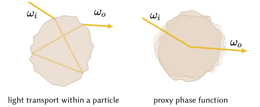
Figure 5. Instead of simulating the full light transport within a particle (left), we use a proxy phase function (right) to aggregate the scattering.

4. Wet materials with volume rendering

With all the parameters defined in the previous section, the wet materials can be rendered by performing Monte Carlo on these particles, including the interactions at the particle interface, light transport within the particles, and the extinction along the ray within the liquid. Apparently, it requires extensive time cost. Hence, we simplify the explicit light transport among the particles by modeling the wet powdered material as a medium. For this, we need to define a phase function for each scattering event (Sec. 4.1), and then formulate the light transport (Sec. 4.2).

4.1. An equivalent phase function

The full light transport within a particle includes reflection, refraction at the particle surface, and the inter-reflection within the particles. To avoid this complex simulation, we derive a phase function as an aggregation at each particle scattering event, as shown in Fig. 5. Since deriving an accurate analytical model for this full simulation is impossible, we propose a data-driven solution by fitting the simulated data with a basis function.

We first introduce two assumptions to simplify the phase function definition without introducing any quality degradation. We assume that the particle is tiny compared to the entire medium, so the points of incident and exit positions are roughly identical. Now, the phase function only depends on the incoming and outgoing directions. However, the four dimensions still raise difficulties on the basis functions for fitting. For this, we have an important observation that the particles have a random distribution, which is a reasonable assumption, as previous works (Kimmel and Baranoski, 2007; Hapke, 2008). This way, the phase function becomes isotropic rather than anisotropic and, therefore, can be defined on the angle between the incoming and outgoing directions.

Then, we choose to use two Gaussians to represent such a one-dimensional phase function, one for forward-scattering and one for backward-scattering:

(1) $$f_{p}(\theta,\mathcal{S}) =w_{1}\cdot G_{1}(\theta;\mu_{1},\sigma_{1})+w_{2}\cdot G_{2}(\theta;\mu_{2},\sigma_{2}),$$

$$G(x;\mu,\sigma) =\frac{1}{\sqrt{2\pi}\sigma}e^{-\frac{(x-\mu)^{2}}{2\sigma^{2}}},$$

where $\theta$ is the angle between the incoming and outgoing directions, $G_{1}$ and $G_{2}$ are two one-dimensional Gaussian functions with parameters $\mu$ as the mean value and $\sigma$ as the variance. $w_{1}$ and $w_{2}$ are the weights for two Gaussians. All these parameters form the parameter set $\mathcal{S}$, which are established by optimization:

(2) $$\mathop{\min}_{\mathcal{S}} \sum_{\theta}(f_{p}(\theta;\mathcal{S})-f_{\mathrm{gt}}(\theta))^{2},$$

where $f_{\mathrm{gt}}(\theta)$ is generated by Monte Carlo simulation, detailed as follows.

We first generate $\omega_{i}$ by sampling on a sphere uniformly w.r.t. the solid angle. Then, we generate the ray’s starting point by sampling a disk that is located at the plane perpendicular to the incoming ray and can cover the entire ellipsoid. Then, we shoot the ray and intersect it with the ellipsoid. If there is no intersection, the ray is discarded; otherwise, we perform the regular path tracing (i.e., sample the visible normal distribution function on the surface to get a microfacet normal, and then decide reflection or refraction with the Fresnel term as the probability) on a microfacet model until leaving the particle surface. This simulation uses one hundred million samples to generate ground truth values. Then, we optimize the Eqn. (2) with the Levenberg-Marquardt algorithm and use the residual sum of squares (RSS) as the loss function. The simulation costs about 1 minute, while the fitting costs 1 second for each material.

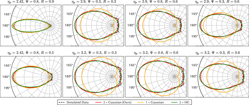
Figure 11. Comparison among two Gaussians (ours), one Gaussian, two HG functions, and the simulated data (GT) on different types of particles and liquid. Our two-Gaussian phase function has the closest match with the GT on all these settings compared to other basis functions.

Our two-Gaussian phase function can match the reference on various parameters, as shown in Fig. 11. Note that our proxy phase function allows multiple types of particles by performing weighted blending on individual fitted phase functions, as shown in Fig. 9.

4.2. Modified RTE for porosity and saturation

Now, we have a simple phase function to define the scattering of powder particles. Then, we derive the formulation required by volume rendering. The radiative transfer equation is usually used to model the light transport within a regular continuous medium, which does not have the desired parameters of porosity and saturation. A related model by Hapke (Hapke, 2008) modifies the original RTE, and enables porosity. We briefly review their formulation and extend it for saturation.

Hapke’s model

The original RTE is defined as:

(3) $$(\omega\cdot\nabla)L(\omega)=-\sigma_{t}L(\omega)+\sigma_{s}\int_{\Omega}f_{p}\left(\omega^{\prime}\cdot\omega\right)L\left(\omega^{\prime}\right)\mathrm{d}\omega^{\prime},$$

where $\sigma_{t}$ and $\sigma_{s}$ are the extinction and scattering coefficients respectively. Note that the dependence on the position in Eqn. (3) is ignored for compactness. The self-emissive term is also omitted, as it’s unnecessary in our case. Then, the typical transmittance can be derived as:

(4) $$T(t)=e^{-\sigma_{t}t}.$$

Hapke (2008) introduced the porosity into the original RTE by distributing particles in a lattice of imaginary cubes, accumulating their transmittance and then replacing the discrete distribution with a continuous distribution, leading to their own transmittance $T_{H}$:

(5) $$T_{H}(t) =Ke^{-K\sigma_{t}t}$$

$$K =-\frac{\ln{(1-\sigma_{t}l)}}{\sigma_{t}l}$$

$$\sigma_{t} =\frac{\left(\frac{3\sqrt{\pi}}{4}\right)^{\frac{2}{3}}\left(1-P\right)^{\frac{2}{3}}}{l}$$

$$l =n^{-\frac{1}{3}},$$

where $K$ is related to $\sigma_{t}$ and the mean distance $l$ between particles. $n$ is the total number of particles per unit volume and $\sigma_{t}$ is established by the porosity and the mean distance. In this way, the parameter porosity is integrated into the RTE.

Our modified RTE

After the powdered materials get wet with a liquid, we need to change the RTE further. Note that when the liquid enters the medium, the distribution of the powder particles does not change and only replaces the fraction of air. Also, we do not consider the air and liquid interaction within the medium. With these two assumptions, we derive the formulation of the transmittance considering both the porosity and saturation:

(6) $$T_{W}(t) =e^{-{\sigma_{t}^{l}}St}\cdot T_{H}(t),$$

where $S$ is the saturation and $\sigma_{t}^{l}$ is the extinction coefficients of the liquid.

5. WetSpongeCake: A BSDF model with porosity and saturation

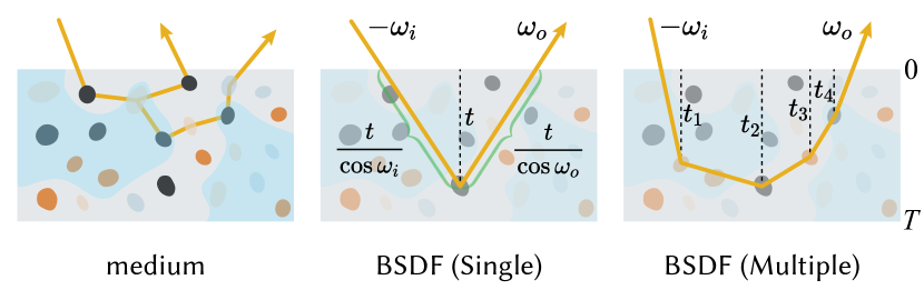
Figure 6. The light transport within a medium is approximated by a surface model, consisting of an analytical single scattering and a Monte Carlo-based multiple scattering by performing the integral along the depth dimension only rather than the entire 3D spatial domain.

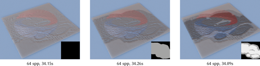
Figure 7. A wet paper with different saturation textures (bottom right). Our method is able to characterize these different kinds of appearances with a low time cost (about 34 seconds) using physical materials, while no existing approaches can achieve this. Medium parameters: $T=0.0017,n=300M,P=0.5,\sigma_{t}^{l}=0$. Particle parameters: $\alpha=(1,1,1),\eta_{l}=1.333$, 70% cellulose + 30% $\text{TiO}_{2}$.

We have already defined the medium, which still requires large sampling rates for convergence. Therefore, we integrate it into the SpongeCake framework by treating the medium as a layer, as shown in Fig. 6. We derive the analytical model for the single scattering, considering both reflection and transmission. Then, we further introduce the multiple scattering and the delta transmission, which complete our full solution.

5.1. Single scattering

The single scattering within a medium with thickness $T$ can be computed by the integral over the depth of the single scattering vertex (Wang et al., 2022b), as shown in Fig. 6. At each single scattering vertex, we compute our two-Gaussian phase function, the extinction of the particles and the liquid, together with cosine terms due to the change of the integration domain. When there are multiple particles in the medium, we blend the phase functions with blending weights, and notate the blended phase function as $\overline{f}_{p}$. Then, the BRDF can be formulated as:

(7) $$f_{r}\left(\omega_{i},\omega_{o}\right)= \int_{0}^{T}K^{2}\frac{\sigma_{s}\overline{f}_{p}\left(\omega_{i}\cdot\omega_{o}\right)}{\cos\omega_{i}\cdot\cos\omega_{o}}$$

$$e^{\left(-\frac{t\left(K\sigma_{t}+{\sigma_{t}^{l}}S\right)}{\cos\omega_{i}}\right)}e^{\left(-\frac{t\left(K\sigma_{t}+{\sigma_{t}^{l}}S\right)}{\cos\omega_{o}}\right)}\mathrm{d}t$$

For briefly, we define several variables:

(8) $$\tau= T\left(K\sigma_{t}+{\sigma_{t}^{l}}S\right)$$

$$\lambda= \frac{K^{2}\sigma_{t}\alpha}{K\sigma_{t}+{\sigma_{t}^{l}}S}.$$

By solving the above equation, replacing $\sigma_{s}=\sigma_{t}\alpha$ and using the above variables, the result is:

(9) $$f_{r}\left(\omega_{i},\omega_{o}\right)=\lambda\frac{\overline{f}_{p}\left(\omega_{i}\cdot\omega_{o}\right)}{\cos\omega_{i}+\cos\omega_{o}}\left(1-e^{-\tau\left(\frac{1}{\cos\omega_{i}}+\frac{1}{\cos\omega_{o}}\right)}\right).$$

Similarly, we also derive the formulation for the transmission, where the incoming and outgoing rays locate at the opposite the surface, leading to a minor difference of the extinction computation:

(10) $$f_{t}\left(\omega_{i},\omega_{o}\right)= \int_{0}^{T}K^{2}\frac{\sigma_{s}\overline{f}_{p}\left(\omega_{i}\cdot\omega_{o}\right)}{\left|\cos\omega_{i}\cdot\cos\omega_{o}\right|}$$

$$e^{\left(-\frac{t\left(K\sigma_{t}+{\sigma_{t}^{l}}S\right)}{\cos\omega_{i}}\right)}e^{\left(-\frac{\left(T-t\right)\left(K\sigma_{t}+{\sigma_{t}^{l}}S\right)}{|\cos\omega_{o}|}\right)}\mathrm{d}t$$

$$= \lambda\frac{\overline{f}_{p}\left(\omega_{i}\cdot\omega_{o}\right)}{\cos\omega_{i}+\cos\omega_{o}}\left(e^{\frac{\tau}{\cos\omega_{o}}}-e^{-\frac{\tau}{\cos\omega_{i}}}\right)$$

Our single scattering is analytical, resulting in a comparable time cost to the microfacet model.

5.2. Other components

With the single scattering, our model can already represent some thin materials. However, it still leads to apparent energy loss for materials with a large thickness relative to their mean free path. Hence, we introduce the multiple scattering.

Multiple scattering

Regarding the multiple scattering, we exploit the position-free Monte Carlo (Guo et al., 2018) as our solution. Although mapping the multiple scattering to a single scattering of modified parameters (Wang et al., 2022b) can further reduce the noise, we leave it for the future work.

Delta transmission

For a thin medium, the light can pass through the medium without any scattering. Some materials have this effect (e.g., paper), while others do not (sand, wood, stone, etc.). This delta function can be computed by the product of transmissions through the medium in the direction $\omega_{i}$, similar to the SpongeCake model.

Importance sampling

Importance sampling is a necessary component for a BSDF. For this, we use a simple solution, by sampling the phase function to generate the outgoing direction, similar to the SpongeCake model.

6. Results

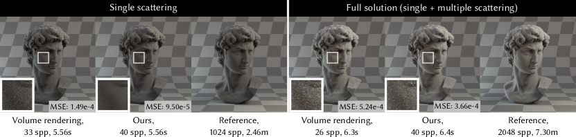
Figure 8. Comparison between our BSDF surface model and the volume rendering with our modified RTE on single scattering and the full solution. The references are rendered with our modified RTE at a high sample rate, where the maximum bounce is set as 1 for the single scattering comparison. In both cases, our BSDF produces results with much less noise and lower error than the volume renderings with equal time. Medium parameters: $T=\infty,n=1M,P=0.5,S=0$, Particle parameters: $\alpha=(0.85,0.85,0.85)$, 50% $\text{CaSO}_{4}$ + 30% $\text{Fe}_{2}\text{O}_{3}$ + 20% $\text{MgSiO}_{3}$.

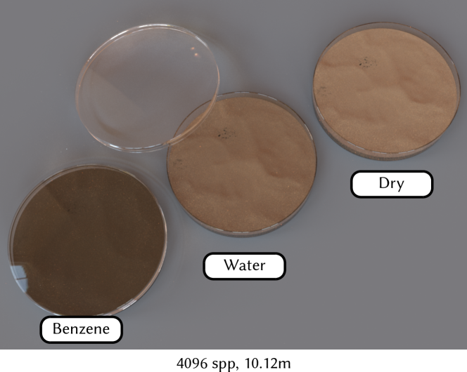
Figure 9. Sand saturated by different liquids. Left: saturated by benzene ($S=0.9,n_{l}=1.501,\sigma_{t}^{l}=0$). Middle: saturated by water ($S=0.9,\eta_{l}=1.333,\sigma_{t}^{l}=0$). Right: dry. Medium parameters: $T=\infty,n=1K,P=0.425$. Particle parameters: $\alpha=$texture, 40% $\text{Fe}_{2}\text{O}_{3}$ + 40% FeO(OH) + 20% $\text{SiO}_{2}$.

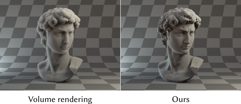
Figure 10. Failure case. Our method cannot handle materials with a large mean free path, leading to a noticeable difference from the volume renderings, similar to all the other position-free based methods (Guo et al., 2018).

We have implemented our algorithm inside the Mitsuba renderer (2010). We also implement our modified RTE, which considers the porosity and saturation as the ground truth (GT), since no other public code is available for wet powdered materials. We use mean square error (MSE) to measure the difference between each method and our modified RTE. All timings in this section are measured on a 2.20GHz Intel i7 (48 cores) with 32 GB of main memory.

Phase function validation

Our two-Gaussian phase function is a critical component of our method. We validate its effectiveness in Fig. 11 by comparing several different basis functions on several types of particles. We compare our two-Gaussian functions, one Gaussian, two HG functions, and the simulated data (performing Monte Carlo for a particle), which we treat as GT. A single-Gaussian function shows the worst match with the simulated data, due to its limited capability. The two-HG function can represent the backward scattering due to the second lobe, but its distribution differs from the simulated data, even for the forward scattering. Our two-Gaussian function can match the GT closely and consistently on all shown particles.

Sculpture scene

We validate the correctness of our single scattering on the Sculpture scene in Fig. 8, where the sculpture is made of three types of particles (50% $\text{CaSO}_{4}$ + 30% $\text{Fe}_{2}\text{O}_{3}$ + 20% $\text{MgSiO}_{3}$) with 1 million particles per unit volume and a grey color ($\alpha=0.85$). The porosity and saturation are set as 0.5 and 0, respectively. In this scene, we consider direct illumination under two area light sources and an environment map. We compare our method against the volume rendering (our modified RTE), where the converged volume rendering result is treated as the ground truth. We find that the result of our single scattering is almost identical to the GT, while has much less noise than the volume rendering with equal time. Then main reason is that our single scattering model is analytical and does not need a random walk. Then, we provide the rendered results of the full solution, consisting of the single and multiple scattering. Our result still exhibits less noise and lower error than volume rendering with equal time. Thanks to the position-free property, although our method needs Monte Carlo simulation for multiple scattering, the integration is performed on the depth rather than the entire spatial domain, significantly reducing noise.

Paper scene

We design a Paper scene with three maps to define the saturation in Fig. 7. We use water ($n_{l}=1.333$) as the liquid with no extinction ($\sigma_{t}^{l}=0$), and the white paper ($\alpha=1$) is made of two particles: 70% cellulose + 30% $\text{TiO}_{2}$. The other parameter settings are $T=0.0017,n=300M,P=0.5$. The saturation maps are shown at the bottom right of each rendered image. This scene is lit by an environment map, considering the global illumination. With all these physical parameters, our single shading model is able to produce the desired and natural effects with a low time cost, which is compatible with the microfacet model. To our knowledge, no existing methods can achieve such a lightweight, physically-based shading model to characterize porosity and saturation.

Sand scene

In this Sand scene (Fig. 9), we show both dry and wet sand, which are filled with water or benzene. The sand consists of three particles (40% $\text{Fe}_{2}\text{O}_{3}$ + 40% FeO(OH) + 20% $\text{SiO}_{2}$) with a spatially-varying albedo, the porosity as 0.425, and the saturation as 0.9. The other parameters for benzene and water are $n_{l}=1.501,\sigma_{t}^{l}=0$ and $n_{l}=1.333,\sigma_{t}^{l}=0$, respectively. We render this scene with both single and multiple scattering under an environment map with global illumination. Our model is able to provide vivid and reasonable results. With the same saturation, benzene should give a darker appearance than the water due to their different refraction indices. Similarly, wet sand looks darker than dry sand. Our model can well characterize both of these effects.

Teaser scene

In Fig. 1, we show several objects with powder materials lit by an environment map, including wet paper, flowerpots, and sculptures. Their parameters are shown in the figure. We use the single scattering for the damp paper and the full solution for others and apply global illumination. Our BSDF can represent a wide range of appearances in the real world with high fidelity, controlled by physical parameters. It is simple and practical, so we believe it can serve as a plugin for existing renderers.

Discussion and limitations

We have identified several limitations of our method. We assume the isotropic particle distribution to simplify the phase function derivation. It is a reasonable assumption for some materials, like clay or sand, but it does not hold for anisotropic materials, like fabrics. Deriving an anisotropic phase function will further increase the capability of our model, and we leave it for future work. Furthermore, similar to previous works (Guo et al., 2018; Wang et al., 2022b), our method inherits the drawbacks from the position-free assumption. For a medium with a large mean free path, the rendering produced by these methods can not match the volume renderings, as shown in Fig.10. However, we believe that the position-free methods can already cover various materials.

7. Conclusion

In this paper, we have presented a surface appearance model – WetSpongeCake for wet powdered materials. At the core of our model is a two-Gaussian phase function that serves as aggregation for light transport within particles and a modified RTE to enable both porosity and saturation. Then, we derive an analytical single scattering under the SpongeCake framework, together with a multiple scattering simulation with the position-free assumption. As a result, our WetSpongeCake model is able to represent various appearances of wet powdered materials with physical parameters (e.g., porosity and saturation), including both reflection and transmission effects. The characterized appearances can naturally match the real world. To our knowledge, no existing methods can achieve such a lightweight and physically based shading model for wet powdered materials.

In the future, we plan to extend the WetSpongeCake model to anisotropic materials to enhance its capability further so the model can also represent that material made of fibers (e.g., fabric). The proposed framework will inspire more material models for natural effects simulation.

References

- (1)
- Bajo et al. (2021) Juan Miguel Bajo, Claudio Delrieux, and Gustavo Patow. 2021. Physically inspired technique for modeling wet absorbent materials. The Visual Computer 37, 8 (2021), 2053–2068.
- Beckmann and Spizzichino (1963) P. Beckmann and A. Spizzichino. 1963. The scattering of electromagnetic waves from rough surfaces. Pergamon Press.
- Bitterli and d’Eon (2022) Benedikt Bitterli and Eugene d’Eon. 2022. A Position-Free Path Integral for Homogeneous Slabs and Multiple Scattering on Smith Microfacets. Computer Graphics Forum 41, 4 (2022), 93–104. https://doi.org/10.1111/cgf.14589
- Bohren (1983) Craig Bohren. 1983. Simple Experiments in Atmospheric Physics: Multiple Scattering at the Beach. Weatherwise 36, 4 (1983), 197–200. https://doi.org/10.1080/00431672.1983.9930144 arXiv:https://doi.org/10.1080/00431672.1983.9930144
- Burley and Studios (2012) Brent Burley and Walt Disney Animation Studios. 2012. Physically-based shading at disney. In Acm Siggraph, Vol. 2012. vol. 2012, 1–7.
- Cook and Torrance (1982) Robert L. Cook and Kenneth E. Torrance. 1982. A Reflectance Model for Computer Graphics. ACM Trans. Graph. 1, 1 (Jan. 1982), 7–24.
- Cui et al. (2023) Yuang Cui, Gaole Pan, Jian Yang, Lei Zhang, Ling-Qi Yan, and Beibei Wang. 2023. Multiple-bounce Smith Microfacet BRDFs using the Invariance Principle. In SIGGRAPH Asia 2023 Conference Papers (SA ’23). Association for Computing Machinery, New York, NY, USA, Article 39, 10 pages. https://doi.org/10.1145/3610548.3618198
- Gamboa et al. (2020) Luis E. Gamboa, Adrien Gruson, and Derek Nowrouzezahrai. 2020. An Efficient Transport Estimator for Complex Layered Materials. Computer Graphics Forum 39, 2 (2020), 363–371.
- Guillén et al. (2020) Ibón Guillén, Julio Marco, Diego Gutierrez, Wenzel Jakob, and Adrien Jarabo. 2020. A General Framework for Pearlescent Materials. Transactions on Graphics (Proceedings of SIGGRAPH Asia) 39, 6 (Nov. 2020). https://doi.org/10.1145/3414685.3417782
- Guo et al. (2018) Yu Guo, Miloš Hašan, and Shuang Zhao. 2018. Position-Free Monte Carlo Simulation for Arbitrary Layered BSDFs. ACM Trans. Graph. 37, 6, Article 279 (Dec. 2018), 14 pages.
- Hapke (1999) Bruce Hapke. 1999. Scattering and Diffraction of Light by Particles in Planetary Regoliths. Journal of Quantitative Spectroscopy and Radiative Transfer 61, 5 (1999), 565–581. https://doi.org/10.1016/S0022-4073(98)00042-9
- Hapke (2008) Bruce Hapke. 2008. Bidirectional reflectance spectroscopy: 6. Effects of porosity. Icarus 195, 2 (2008), 918–926. https://doi.org/10.1016/j.icarus.2008.01.003
- Heitz and d’Eon (2014) Eric Heitz and Eugene d’Eon. 2014. Importance Sampling Microfacet-Based BSDFs using the Distribution of Visible Normals. Computer Graphics Forum 33, 4 (2014), 103–112.
- Heitz et al. (2016) Eric Heitz, Johannes Hanika, Eugene d’Eon, and Carsten Dachsbacher. 2016. Multiple-Scattering Microfacet BSDFs with the Smith Model. ACM Trans. Graph. 35, 4, Article 58 (July 2016), 14 pages.
- Hnat et al. (2006) Kevin Hnat, Damien Porquet, Stéphane Merillou, and Djamchid Ghazanfarpour. 2006. Real-Time Wetting of Porous Media. MG&V 15, 3 (jan 2006), 401–413.
- Jakob (2010) Wenzel Jakob. 2010. Mitsuba renderer. http://www.mitsuba-renderer.org.
- Jensen et al. (1999) Henrik Wann Jensen, Justin Legakis, and Julie Dorsey. 1999. Rendering of Wet Materials. In Proceedings of the 10th Eurographics Conference on Rendering (EGWR’99). Eurographics Association, Goslar, DEU, 273–282.
- Kimmel and Baranoski (2007) BradleyW. Kimmel and Gladimir V.G. Baranoski. 2007. A novel approach for simulating light interaction with particulate materials: application to the modeling of sand spectral properties. Opt. Express 15, 15 (Jul 2007), 9755–9777. https://doi.org/10.1364/OE.15.009755
- Kulla and Conty (2017) Christopher Kulla and Alejandro Conty. 2017. Physically Based Shading in Theory and Practice - Revisiting Physically Based Shading at Imageworks. http://blog.selfshadow.com/publications/s2017-shading-course/.
- Lee et al. (2018) Joo Lee, Adrián Jarabo, Daniel Jeon, Diego Gutiérrez, and Min Kim. 2018. Practical multiple scattering for rough surfaces. ACM Trans. Graph. 37, Article 175 (Dec. 2018), 12 pages.
- Lekner and Dorf (1988) John Lekner and Michael C. Dorf. 1988. Why some things are darker when wet. Appl. Opt. 27, 7 (Apr 1988), 1278–1280. https://doi.org/10.1364/AO.27.001278
- Lu et al. (2006) Jianye Lu, Athinodoros S. Georghiades, Holly Rushmeier, Julie Dorsey, and Chen Xu. 2006. Synthesis of material drying history: phenomenon modeling, transferring and rendering. In ACM SIGGRAPH 2006 Courses (SIGGRAPH ’06). Association for Computing Machinery, New York, NY, USA, 6–es. https://doi.org/10.1145/1185657.1185726
- Lucas et al. (2023) Simon Lucas, Mickael Ribardiere, Romain Pacanowski, and Pascal Barla. 2023. A Micrograin BSDF Model for the Rendering of Porous Layers. In SIGGRAPH Asia 2023 Conference Papers (SA ’23). Association for Computing Machinery, New York, NY, USA, Article 40, 10 pages. https://doi.org/10.1145/3610548.3618241
- Meng et al. (2015) Johannes Meng, Marios Papas, Ralf Habel, Carsten Dachsbacher, Steve Marschner, Markus Gross, and Wojciech Jarosz. 2015. Multi-scale modeling and rendering of granular materials. ACM Trans. Graph. 34, 4, Article 49 (jul 2015), 13 pages. https://doi.org/10.1145/2766949
- Merillou et al. (2000) S. Merillou, J.-M. Dischler, and D. Ghazanfarpour. 2000. A BRDF postprocess to integrate porosity on rendered surfaces. IEEE Transactions on Visualization and Computer Graphics 6, 4 (2000), 306–318. https://doi.org/10.1109/2945.895876
- Moon et al. (2007) Jonathan T. Moon, Bruce Walter, and Stephen R. Marschner. 2007. Rendering discrete random media using precomputed scattering solutions. In Proceedings of the 18th Eurographics Conference on Rendering Techniques (EGSR’07). Eurographics Association, Goslar, DEU, 231–242.
- Müller et al. (2016) Thomas Müller, Marios Papas, Markus Gross, Wojciech Jarosz, and Jan Novák. 2016. Efficient rendering of heterogeneous polydisperse granular media. ACM Trans. Graph. 35, 6, Article 168 (dec 2016), 14 pages. https://doi.org/10.1145/2980179.2982429
- Peltoniemi and Lumme (1992) Jouni I. Peltoniemi and Kari Lumme. 1992. Light scattering by closely packed particulate media. J. Opt. Soc. Am. A 9, 8 (Aug 1992), 1320–1326. https://doi.org/10.1364/JOSAA.9.001320
- Shkuratov et al. (1999) Yurij Shkuratov, Larissa Starukhina, Harald Hoffmann, and Gabriele Arnold. 1999. A Model of Spectral Albedo of Particulate Surfaces: Implications for Optical Properties of the Moon. Icarus 137, 2 (1999), 235–246. https://doi.org/10.1006/icar.1998.6035
- Turquin (2019) Emmanuel Turquin. 2019. Practical multiple scattering compensation for microfacet models. https://blog.selfshadow.com/publications/turquin/ms_comp_final.pdf.
- Twomey et al. (1986) Sean A. Twomey, Craig F. Bohren, and John L. Mergenthaler. 1986. Reflectance and albedo differences between wet and dry surfaces. Appl. Opt. 25, 3 (Feb 1986), 431–437. https://doi.org/10.1364/AO.25.000431
- Walter et al. (2007) Bruce Walter, Stephen R. Marschner, Hongsong Li, and Kenneth E. Torrance. 2007. Microfacet Models for Refraction through Rough Surfaces. In Rendering Techniques (proc. EGSR 2007). The Eurographics Association, 195–206.
- Wang et al. (2022a) Beibei Wang, Wenhua Jin, Jiahui Fan, Jian Yang, Nicolas Holzschuch, and Ling-Qi Yan. 2022a. Position-Free Multiple-Bounce Computations for Smith Microfacet BSDFs. ACM Trans. Graph. 41, 4, Article 134 (jul 2022), 14 pages.
- Wang et al. (2022b) Beibei Wang, Wenhua Jin, Miloš Hašan, and Ling-Qi Yan. 2022b. SpongeCake: A Layered Microflake Surface Appearance Model. ACM Trans. Graph. 42, 1, Article 8 (sep 2022), 16 pages. https://doi.org/10.1145/3546940
- Xia et al. (2020) Mengqi (Mandy) Xia, Bruce Walter, Christophe Hery, and Steve Marschner. 2020. Gaussian Product Sampling for Rendering Layered Materials. Computer Graphics Forum 39, 1 (2020), 420–435.
- Xie and Hanrahan (2018) Feng Xie and Pat Hanrahan. 2018. Multiple Scattering from Distributions of Specular V-Grooves. ACM Trans. Graph. 37, 6, Article 276 (2018), 14 pages.
- Ångström (1925) Anders Ångström. 1925. The Albedo of Various Surfaces of Ground. Geografiska Annaler 7 (1925), 323–342. http://www.jstor.org/stable/519495