A semidefinite programming approach for robust elliptic localization

Abstract

This short communication addresses the problem of elliptic localization with outlier measurements, whose occurrences are prevalent in various location-enabled applications and can significantly compromise the positioning performance if not adequately handled. In contrast to the reliance on $M$-estimation adopted in the majority of existing solutions, we take a different path, specifically exploring the worst-case robust approximation criterion, to bolster resistance of the elliptic location estimator against outliers. From a geometric standpoint, our method boils down to pinpointing the Chebyshev center of the feasible set determined by the available bistatic ranges with bounded measurement errors. For a practical approach to the associated min-max problem, we convert it into the well-established convex optimization framework of semidefinite programming (SDP). Numerical simulations confirm that our SDP-based technique can outperform a number of existing elliptic localization schemes in terms of positioning accuracy in Gaussian mixture noise, a common type of impulsive interference in the context of range-based localization.

1 Introduction

The last decade has witnessed a widespread adoption of elliptic localization techniques across various location-based applications, in line with the contemporary proliferation of multistatic systems like distributed multiple-input multiple-output (MIMO) radar, sonar, and wireless sensor networks [1]. Such systems are typically composed of a number of spatially separated transmitters and receivers, whose positions $\bm{t}_{m}=[x_{m}^{t},y_{m}^{t}]^{T}$ (for $m=1,...,M$) and $\bm{s}_{l}=[x_{l},y_{l}]^{T}$ (for $l=1,...,L$), respectively, are known in advance. Mathematically, elliptic localization involves an estimation problem, aimed at ascertaining the location of a signal-reflecting/relaying target, $\bm{x}=[x,y]^{T}$, by utilizing the sensor-collected bistatic ranges (BRs):

$$\hat{r}_{m,l}={\|\bm{x}-\bm{t}_{m}\|}_{2}+{\|\bm{x}-\bm{s}_{l}\|}_{2}+e_{m,l},$$

$$~{}m=1,...,M,~{}l=1,...,L,$$ (1)

where ${\|\cdot\|}_{2}$ denotes the $\ell_{2}$-norm and $\{e_{m,l}\}$ represent the BR measurement errors. Over the past several years, numerous practical and theoretically sound elliptic location estimators have been developed to accomplish this task. We will provide a brief summary of the relevant works as follows.

When $\{e_{m,l}\}$ follow zero-mean Gaussian distributions, least squares (LS)-based location estimators, whether linear or nonlinear, are employed to attain statistical efficiency from the available BRs [2]. Linear LS approaches are perhaps the most extensively studied in the literature, thanks to the computational convenience they offer. By converting the nonlinear BR expressions into models linear in $\bm{x}$, these elliptic localization techniques allow for closed-form solutions [3, 4, 5, 6, 7] or, even when not strictly closed-form due to the inclusion of constraints describing how $\bm{x}$ is related to certain nuisance parameter(s), solutions with computational load inconsequential for real-time location-based applications [8]. On the other hand, current progress in advanced iterative optimization solvers also enables the direct implementation of nonlinear LS position estimators in a computationally efficient manner. Within the particular field of elliptic localization, solvers of this kind encompass Lagrange-type iterative algorithms built upon Lagrange programming neural network (LPNN) [9] and alternating direction method of multipliers (ADMM) [10]. In addition, the constrained LS problems formulated for elliptic localization in Gaussian noise can be solved by means of semidefinite programming (SDP) [11, 12], a well-established convex optimization methodology.

More recently, there have been a growing number of investigations delving into elliptic localization in scenarios of greater practical significance, specifically, in the presence of outlier measurements. The justification for such research lies in the fact that the daily operations of localization systems, notably in various location-enabled applications, are often impacted by adverse environmental factors, including non-line-of-sight (NLOS) signal propagation and interference [13]. They will contribute to non-Gaussian $\{e_{m,l}\}$, translate to outliers in $\{\hat{r}_{m,l}\}$, and eventually degrade the reliability of the conventional LS location estimators [14].

Perhaps the most widely adopted strategy in the existing literature to handle outlying BR observations is to exploit principles of robust $M$-estimation [15, 16, 17, 18, 19, 20, 21]. Approaches falling within this category operate by replacing the non-outlier-resistant $\ell_{2}$ loss in the LS formulation with cost functions that exhibit reduced sensitivity to deviating samples. In the pioneering research [15], a correntropy-induced loss was introduced as the substitute for its $\ell_{2}$ counterpart, and a half-quadratic algorithm was devised to tackle the associated optimization problem. Later on, there have also been successful applications of more computationally lightweight iterative schemes to address the least absolute deviation (LAD)/$\ell_{1}$-minimization formulations for robust elliptic localization. These include the LPNN in [16], the iterative message passing (MP) algorithm in [17], and the ADMM in [18, 19]. Expanding on the LPNN in [16], the authors of [20] developed an iteratively reweighted LAD (IRLAD) scheme tailored for $\ell_{p}$-minimization, particularly when $p=0$, with the expectation of enhancing outlier-robustness of the elliptic position estimator in specific scenarios. In our latest study [21], we incorporated majorization–minimization (MM) into an iteratively reweighted LS (IRLS) framework to achieve statistical optimality in the case of stably distributed $\{e_{m,l}\}$ through least $\ell_{p}$-norm estimation.

The contribution of this work is threefold, as outlined below:

i) In contrast to the commonplace use of $M$-estimators in the existing solutions [15, 16, 17, 18, 19, 20, 21], we opt for a different path to perform robust elliptic localization. Our formulation is rooted in the worst-case robust approximation criterion [22], presenting itself as a min-max optimization problem. In essence, the maximum possible $\bm{x}$-estimation error under uncertainty specified by $\{\hat{r}_{m,l}\}$ with bounded $\{e_{m,l}\}$, is minimized, rather than a certain robust loss function as in the $M$-estimators. This, from a geometric perspective, corresponds to locating the Chebyshev center within the associated feasible set.

ii) Since determining the Chebyshev center poses an NP-hard problem except in certain special cases [23], we reshape the original min-max formulation into an SDP framework. In addition, we analyze the complexity for implementing the presented SDP-based approach.

iii) Simulation results are provided to validate our proposal and demonstrate its superior performance compared to several off-the-shelf elliptic localization methods.

2 Problem statement and error modeling

In this section, we formulate the robust location estimation problem by following the worst-case approximation criterion. Furthermore, we detail the measurement error modeling strategy under consideration.

In order to employ such a set-based, worst-case approach, it is necessary to first describe the uncertainty (to be maximized) across a set of possible values, namely, the feasible set [22]. To accomplish this, we make the additional assumption that the magnitude of the BR measurement errors $\{e_{m,l}\}$ is upper bounded by some given constant $\rho>0$:

$${}|e_{m,l}|\leq\rho.$$ (2)

It is worth highlighting that similar assumptions have been commonly adopted in the literature concerning range-based localization methods, such as those utilizing the received signal strength [24], time-of-arrival [24, 25, 26], and time-difference-of-arrival [27, 28] measurements. These requirements prove to be milder when compared to precisely characterizing the corresponding statistical distributions and, in practical terms, the error upper bound can be readily estimated during the calibration and commissioning stage using training data [27].

Using $\bm{z}\in\mathbb{R}^{2}$ to denote a feasible target location estimate, we can now express the following min-max problem:

$${}\min_{\bm{x}}\max_{\bm{z}\in\mathcal{C}_{\bm{z}}}{\|\bm{x}-\bm{z}\|}_{2},$$ (3)

where

$$\mathcal{C}_{\bm{z}}= \big{\{}\bm{z}\in\mathbb{R}^{H}\big{|}\underline{r}_{m,l}\leq{\|\bm{z}-\bm{t}_{m}\|}_{2}+{\|\bm{z}-\bm{s}_{l}\|}_{2}\leq\overline{r}_{m,l},$$

$$~{}m=1,...,M,~{}l=1,...,L\big{\}},$$ (4a)

$$\underline{r}_{m,l}=\hat{r}_{m,l}-\rho,~{}m=1,...,M,~{}l=1,...,L,$$ (4b)

$$\overline{r}_{m,l}=\hat{r}_{m,l}+\rho,~{}m=1,...,M,~{}l=1,...,L.$$ (4c)

Here, $\mathcal{C}_{\bm{z}}$ is the feasible set determined according to (1) and (2), which amounts to the area where the ellipses defined by (4a) intersect.

The geometric interpretation of (3) is to identify the Chebyshev center nestled within $\mathcal{C}_{\bm{z}}$, viz., the center of the minimal-radius circle enclosing $\mathcal{C}_{\bm{z}}$.

In this contribution, we assume that $\{e_{m,l}\}$ are independent and identically distributed and follow two-component Gaussian mixture impulsive distribution [29]:

$$e=\beta\mathcal{N}(\mu,\sigma^{2})+(1-\beta)\mathcal{N}(\check{\mu},\check{\sigma}^{2}),$$ (5)

where $e$ is the random variable being characterized and $\beta$ specifies the proportions in the two-component mixture. $\mathcal{N}$ denotes the standard Gaussian distribution. $\check{\mu}$ and $\check{\sigma}$ are the mean and standard deviation of the second Gaussian mixture component (to which an impulsive $e$ and an associated outlier measurement are attributed), respectively. In contrast, $\mu$ and $\sigma$ correspond to their counterparts associated with the first Gaussian mixture component.

The error modeling option (5) can offer certain advantages in the realm of localization [29]. This is owing to its compatibility and alignment with the superposition form commonly observed in measurement errors when they are introduced into location data acquired under NLOS conditions. The NLOS propagation of signals is a ubiquitous adverse environmental factor that touches on numerous positioning applications [13]. Such a superposition, typically, manifests itself as composite of a lower-level Gaussian disturbance component stemming from thermal fluctuations and a nonnegative random variable representing the NLOS bias [13, 29].

3 SDP formulation and complexity analysis

While its structure is clear and comprehensible, dealing with the problem (3) can be challenging due to the following two reasons. First, the task of determining the Chebyshev center is itself an NP-hard problem except in certain special cases [23]. Second, the presence of multiple local minima and/or maxima makes the optimization process for min-max formulations more complex compared to many other standard optimization problems. In this section, instead of directly addressing (3), we will cast it as an SDP problem that can be easier to solve.

Let us begin by transforming the min-max formulation (3) into the following epigraph-form expression, based on its geometric interpretation described earlier:

$${}\min_{\breve{\bm{x}},\bm{z},\bm{\gamma},t}t,~{}~{}\textup{s.t.}~{}\bm{z}=\breve{\bm{x}}+\bm{\gamma},~{}{\|\bm{\gamma}\|}_{2}\leq t,~{}\bm{z}\in\mathcal{C}_{\bm{z}},$$ (6)

where $\breve{\bm{x}}\in\mathbb{R}^{2}$ is the variable vector for the Chebyshev center of our interest, $\bm{z}=\breve{\bm{x}}+\bm{\gamma}$ defines a circle centered at $\breve{\bm{x}}$ with a radius ${\|\bm{\gamma}\|}_{2}$, $\bm{\gamma}\in\mathbb{R}^{2}$, and $t\in\mathbb{R}$. Rewriting the inequalities in (4a) in quadratic form yields

$$\underline{r}_{m,l}^{2}+g_{m}^{t}-2\underline{r}_{m,l}d_{m}^{t} =(\underline{r}_{m,l}-d_{m}^{t})^{2}\leq g_{l}^{s},$$ (7a)

$$\overline{r}_{m,l}^{2}+g_{m}^{t}-2\overline{r}_{m,l}d_{m}^{t} =(\overline{r}_{m,l}-d_{m}^{t})^{2}\geq g_{l}^{s},$$ (7b)

where

$$g_{m}^{t} =(d_{m}^{t})^{2}={\|\bm{z}-\bm{t}_{m}\|}_{2}^{2},~{}m=1,...,M,$$ (8a)

$$g_{l}^{s} ={\|\bm{z}-\bm{s}_{l}\|}_{2}^{2},~{}l=1,...,L.$$ (8b)

Similarly, we re-express ${\|\bm{\gamma}\|}_{2}\leq t$ as

$${\|\bm{\gamma}\|}_{2}^{2}\leq t^{2},~{}t\geq 0,$$ (9)

which is equivalent to

$${}\begin{bmatrix}t\bm{I}_{2}&\bm{\gamma}\\ \bm{\gamma}^{T}&t\end{bmatrix}\succeq\bm{0}_{3\times 3},~{}t\geq 0.$$ (10)

With these reformulations, the constrained optimization problem (6) now reads

$$\min_{\breve{\bm{x}},\bm{z},\bm{\gamma},t,\{d_{m}^{t}\},\{g_{m}^{t}\},\{g_{l}^{s}\},\lambda}t$$

s.t. $$\bm{z}=\breve{\bm{x}}+\bm{\gamma},$$ (11a)

$$\textup{(\ref{cons_innercir})},$$

$$\underline{r}_{m,l}^{2}+g_{m}^{t}-2\underline{r}_{m,l}d_{m}^{t}\leq g_{l}^{s},~{}\forall(m,l),$$ (11b)

$$\overline{r}_{m,l}^{2}+g_{m}^{t}-2\overline{r}_{m,l}d_{m}^{t}\geq g_{l}^{s},~{}\forall(m,l),$$ (11c)

$$g_{m}^{t}=\begin{bmatrix}\bm{t}_{m}\\ -1\end{bmatrix}^{T}\begin{bmatrix}\bm{I}_{2}&\bm{z}\\ \bm{z}^{T}&\lambda\end{bmatrix}\begin{bmatrix}\bm{t}_{m}\\ -1\end{bmatrix},~{}m=1,...,M,$$ (11d)

$$g_{l}^{s}=\begin{bmatrix}\bm{s}_{l}\\ -1\end{bmatrix}^{T}\begin{bmatrix}\bm{I}_{2}&\bm{z}\\ \bm{z}^{T}&\lambda\end{bmatrix}\begin{bmatrix}\bm{s}_{l}\\ -1\end{bmatrix},~{}l=1,...,L,$$ (11e)

$$\lambda=\bm{z}^{T}\bm{z},$$ (11f)

$$g_{m}^{t}=(d_{m}^{t})^{2},$$ (11g)

where $\lambda\in\mathbb{R}$ is an additional variable representing the squared Euclidean distance for $\bm{z}$.

The non-affine equality constraints (11f) and (11g) contribute to the nonconvexity of (11). By relaxing them to

$${}\begin{bmatrix}\bm{I}_{2}&\bm{z}\\ \bm{z}^{T}&\lambda\end{bmatrix}\succeq\bm{0}_{3\times 3}$$ (12)

and

$${}\begin{bmatrix}1&d_{m}^{t}\\ d_{m}^{t}&g_{m}^{t}\end{bmatrix}\succeq\bm{0}_{2\times 2},~{}m=1,...,M,$$ (13)

where $\bm{A}\succeq\bm{0}_{a\times a}$ means that the $a\times a$ symmetric matrix $\bm{A}$ is positive semidefinite, we obtain an SDP formulation:

$$\min_{\breve{\bm{x}},\bm{z},\bm{\gamma},t,\{d_{m}^{t}\},\{g_{m}^{t}\},\{g_{l}^{s}\},\lambda}t$$

s.t. $$\textup{(\ref{cons_innercir})},~{}\textup{(\ref{cons_zxgamma})--(\ref{cons_gls})},~{}\textup{(\ref{cons_lambda})},~{}\textup{(\ref{cons_dmt})}.$$ (14)

The SDP problem (3) falls into the domain of convex optimization and, therefore, can be easily solved using interior-point algorithms with a worst-case complexity on the order of [27]

$$\sqrt{\sum_{n=1}^{N_{\textup{SD}}}D_{\textup{SD,n}}}\!\left(\!N_{\textup{Var}}^{2}\sum_{n=1}^{N_{\textup{SD}}}D_{\textup{SD,n}}^{2}\!+\!N_{\textup{Var}}\sum_{n=1}^{N_{\textup{SD}}}D_{\textup{SD,n}}^{3}\!+\!N_{\textup{Var}}^{3}\!\right)\!\log\big{(}\tfrac{1}{\nu}\big{)},$$ (15)

where $N_{\textup{SD}}$, $D_{\textup{SD,n}}$, $N_{\textup{Var}}$, and $\nu$ denote the number of semidefinite cone constraints, the dimension of the $n$th semidefinite cone constraint, the number of optimization variables, and the precision, respectively. It is evident that $N_{\textup{SD}}=5+2ML+2M+L$ and $N_{\textup{Var}}=8+2M+L$ in this particular case. Specifically, there are $3+2ML+M+L$ semidefinite cone constraint sized 1, $M$ semidefinite cone constraint sized 2, and 2 semidefinite cone constraint sized 3. As a result, the worst-case complexity for addressing (3) via interior-point methods is $\mathcal{O}((M+L)^{2}(ML)^{1.5})$. In order to illustrate the scale of this complexity, we include Table 1, where the complexities of several existing robust elliptic localization methods [21] are also showcased. These approaches will be contrasted with our proposed SDP-based technique (termed min-max) in the simulations in Section 4. In Table 1, $N_{\textup{LPNN}}$, $N_{\textup{MP}}$, $N_{\textup{IRLAD}}$, $N_{\textup{IRLS}}$, and $N_{\textup{MM}}$ represent the discrete realization steps for LPNN (typically several thousands), the number of MP iterations (usually several tens), the number of IRLAD iterations (usually several tens), the number of IRLS iterations (usually several tens), and the number of MM iterations (usually a few), respectively. It is clear that min-max remains computationally competitive in typical elliptic localization configurations, where the values of $M$ and $L$ are not very large in magnitude in most cases [1].

Table 1: Summary of several representative robust elliptic localization methods and our proposal

Method	Description	Complexity
$\ell_{1}$-LPNN [16]	LAD estimator, implemented via LPNN	$\mathcal{O}(N_{\textup{LPNN}}(M+L))$
MP [17]	LAD estimator, implemented via iterative MP	$\mathcal{O}(N_{\textup{MP}}(ML))$
$\ell_{0}$-IIRW [20]	$\ell_{p}$ estimator with $p=0$, implemented via LPNN-based IRLAD	$\mathcal{O}(N_{\textup{IRLAD}}N_{\textup{LPNN}}(M+L))$
$\ell_{1.5}$-IRLS [21]	$\ell_{p}$ estimator with $p=1.5$, implemented via MM-based IRLS	$\mathcal{O}(N_{\textup{IRLS}}N_{\textup{MM}}(ML))$
min-max	Proposed worst-case robust approximation formulation, relaxed as an SDP problem	$\mathcal{O}((M+L)^{2}(ML)^{1.5})$

4 Numerical results

In this section, we conduct numerical tests on a laptop equipped with a 2.8 GHz CPU and 8 GB of RAM to evaluate the performance of min-max (code available at https://github.com/w-x-xiong/min-max). For simulation purposes, we employ a distributed MIMO radar system comprising $M=3$ transmitters and $L=4$ receivers, with their respective positions detailed as follows: $\bm{t}_{1}=[-200,-300]^{T}$ m, $\bm{t}_{2}=[-200,300]^{T}$ m, $\bm{t}_{3}=[200,300]^{T}$ m, $\bm{s}_{1}=[-450,-450]^{T}$ m, $\bm{s}_{2}=[450,450]^{T}$ m, $\bm{s}_{3}=[0,600]^{T}$ m, and $\bm{s}_{4}=[600,0]^{T}$ m. The target is located at $\bm{x}=[100,100]^{T}$ m. We assess the positioning accuracy of min-max by comparing its root-mean-square error (RMSE):

$${}\textup{RMSE}=\sqrt{\tfrac{1}{N_{\textup{MC}}}\sum_{n=1}^{N_{\textup{MC}}}{\|\tilde{\bm{x}}^{\{n\}}-\bm{x}\|}_{2}^{2}}$$ (16)

to that of the approaches from Table 1 and the following two LS-based elliptic localization schemes: a) the constrained weighted LS estimator presented in [8], allowing for an exact solution (termed exact) and b) the nonlinear LS estimator directly implemented through the LPNN [9] (termed $\ell_{2}$-LPNN). In (16), $\tilde{\bm{x}}^{\{n\}}$ represents the target location estimate in the $n$th Monte Carlo (MC) run and $N_{\textup{MC}}$ denotes the number of ensemble MC runs, which is fixed at 100 in our simulations. $\{e_{m,l}\}$ are generated based on the Gaussian mixture impulsive noise modeling strategy in (5). Regarding the implementation of min-max, we solve the associated SDP problem (3) using the MATLAB toolbox CVX [30], with the SDPT3 solver. Unless stated otherwise, the error upper bound required by min-max is exactly provided.

Figure 1: RMSE versus $\beta$ when $\mu=0$, $\sigma=1$ m, $\check{\mu}=20$ m, and $\check{\sigma}=1$ m.

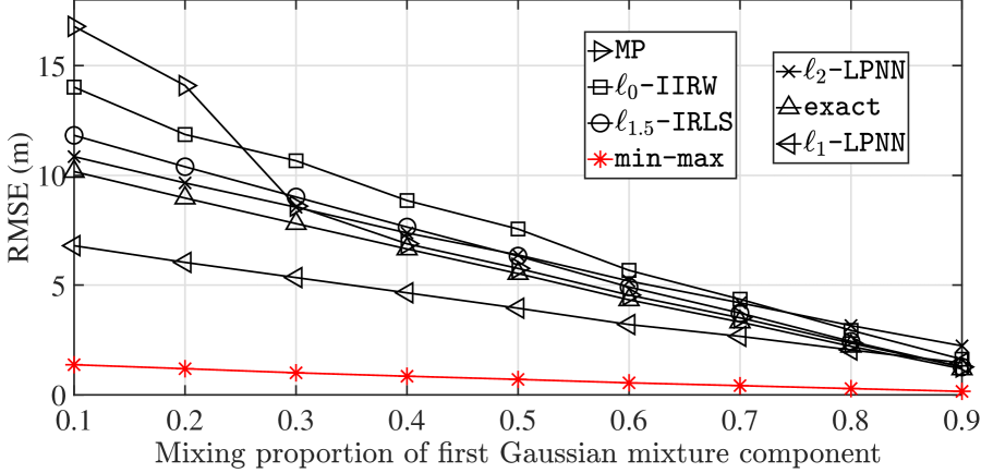
In our first experiment, we vary the proportion of the first Gaussian mixture component, $\beta$, from 0.1 to 0.9, while keeping other parameters in (5) fixed: $\mu=0$, $\sigma=1$ m, $\check{\mu}=20$ m, and $\check{\sigma}=1$ m. Parameter setups with a progressively increasing $\beta$, as indicated by (5), give rise to scenarios in which the likelihood of NLOS conditions gradually decreases from high to low probability. Fig. 1 depicts the corresponding RMSE results, highlighting that min-max consistently outperforms the remaining approaches and delivers the highest positioning accuracy across the entire $\beta$-region under investigation. Also apparent from Fig. 1 is the improvement in the performance of all estimators as $\beta$ increases, with $\ell_{1}$-LPNN emerging as the second-best solution for $\beta\leq 0.8$.

Figure 2: RMSE versus $\check{\mu}$ when $\beta=0.5$, $\mu=0$, $\sigma=1$ m, and $\check{\sigma}=1$ m.

Figure 3: RMSE versus $\check{\sigma}$ when $\beta=0.5$, $\mu=0$, $\sigma=1$ m, and $\check{\mu}=20$ m.

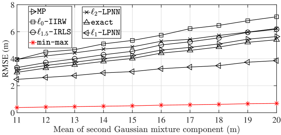
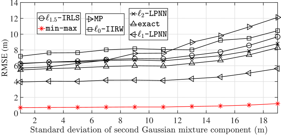
Fig. 2 illustrates how the RMSE varies with the mean of the second Gaussian mixture component, $\check{\mu}$, limited to the interval $[11,20]$ m. These examinations are carried out under the fixed parameters of $\beta=0.5$, $\mu=0$, $\sigma=1$ m, and $\check{\sigma}=1$ m. Such a configuration defines test scenarios where line-of-sight (LOS) links distinctly stand out from their NLOS counterparts. Additionally, for a specific link, the probabilities of encountering LOS and NLOS conditions are evenly split at 50/50. In Fig. 2, there is a clear hierarchy in RMSE values among the seven estimators within the specific $\check{\mu}$-region we are investigating: our proposed method min-max is the lowest, followed by $\ell_{1}$-LPNN, exact, MP, $\ell_{1.5}$-IRLS, $\ell_{2}$-LPNN, and $\ell_{0}$-IIRW, in that order. With an increase in $\check{\mu}$, the RMSE exhibits a consistent upward trend across all schemes. Subsequently, in Fig. 3, the results of RMSE versus the standard deviation of the second Gaussian mixture component, $\check{\sigma}$, are depicted under the specified conditions of $\beta=0.5$, $\mu=0$, $\sigma=1$ m, and $\check{\mu}=20$ m. For each approach, when the $\check{\sigma}$ value exceeds a certain level, the trend of RMSE rising with increasing $\check{\sigma}$ becomes discernible. Again, min-max demonstrates a performance advantage in RMSE compared to others across the entire parameter range we are examining.

Figure 4: RMSE versus $\sigma$ when $\beta=1$ and $\mu=0$.

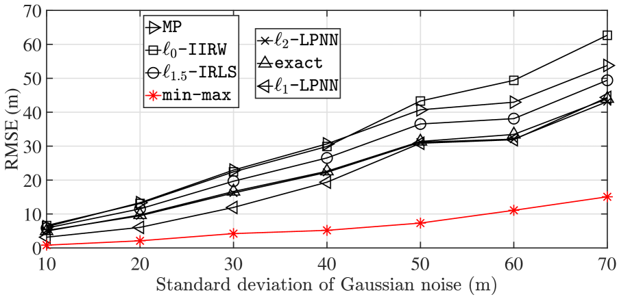
While the above experiments focused on elliptic localization in NLOS environments, there is also a research curiosity in assessing how well our proposed technique functions in noise situations characterized solely by zero-mean Gaussian distributions (i.e., where the adverse environmental factors are absent). To delve into this, Fig. 4 plots the RMSE versus the standard deviation of the first Gaussian mixture component, $\sigma$, with $\beta$ set to 1 and $\mu$ at 0. We see that min-max continues to distinguish itself as the optimal solution in terms of RMSE.

Figure 5: RMSE versus $\hat{\rho}/\rho$ when $\beta=0.5$, $\mu=0$, $\sigma=1$ m, $\check{\mu}=20$ m, and $\check{\sigma}=1$ m.

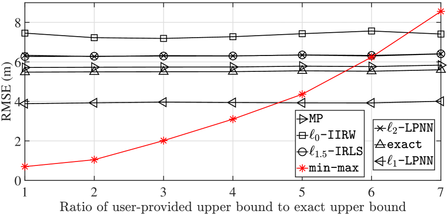
Different from the ideal scenarios discussed earlier, where min-max operated with the exact error upper bound $\rho$, we now investigate min-max’s sensitivity to the exactness of the user-provided upper bound, $\hat{\rho}$, by plotting the RMSE in relation to $\hat{\rho}/\rho$. The error-characterizing parameters in (5) are set as $\beta=0.5$, $\mu=0$, $\sigma=1$ m, $\check{\mu}=20$ m, and $\check{\sigma}=1$ m, and the obtained RMSE results are depicted in Fig. 5. We see that min-max maintains a high level of competitiveness in positioning accuracy as long as $\hat{\rho}/\rho$ is not excessively large, e.g., when $\hat{\rho}/\rho\leq 5$.

5 Conclusion

In this short communication, we have presented a new formulation for elliptic localization with outliers based on the worst-case robust approximation criterion. Geometrically speaking, our goal was to locate the Chebyshev center given a feasible set defined according to (i) the known sensor positions, (ii) the available BR measurements, and (iii) the maximum limit for the magnitude of BR measurement errors. Such a problem, initially, posed itself as a min-max optimization task. Instead of directly addressing this challenging min-max formulation, we conducted a transformation based on its geometric interpretation and shifted our focus to an SDP approach that holds greater practical significance. Simulation results affirm the robustness of our proposed elliptic localization method to outliers, demonstrating an overall improvement compared to a number of existing solutions.

References

- [1] L. Rui and K. C. Ho, “Elliptic localization: Performance study and optimum receiver placement,” IEEE Trans. Signal Process., vol. 62, no. 18, pp. 4673–4688, Sep. 2014.
- [2] S. M. Kay, Fundamentals of Statistical Signal Processing: Estimation Theory, vol. 2. Cliffs, NJ, USA: Prentice-Hall, 1998.
- [3] M. Dianat, M. R. Taban, J. Dianat, and V. Sedighi, “Target localization using least squares estimation for MIMO radars with widely separated antennas,” IEEE Trans. Aerosp. Electron. Syst., vol. 49, no. 4, pp. 2730–2741, Oct. 2013.
- [4] A. Noroozi and M. A. Sebt, “Target localization from bistatic range measurements in multi-transmitter multi-receiver passive radar,” IEEE Signal Process. Lett., vol. 22, no. 12, pp. 2445–2449, Dec. 2015.
- [5] M. Einemo and H. C. So, “Weighted least squares algorithm for target localization in distributed MIMO radar,” Signal Process., vol. 115, pp. 144–150, Oct. 2015.
- [6] R. Amiri, F. Behnia, and H. Zamani, “Asymptotically efficient target localization from bistatic range measurements in distributed MIMO radars,” IEEE Signal Process. Lett., vol. 24, no. 3, pp. 299–303, Mar. 2017.
- [7] A. Noroozi, M. A. Sebt, S. M. Hosseini, R. Amiri, and M. M. Nayebi, “Closed-form solution for elliptic localization in distributed MIMO radar systems with minimum number of sensors,” IEEE Trans. Aerosp. Electron. Syst., vol. 56, no. 4, pp. 3123–3133, Aug. 2020.
- [8] R. Amiri, F. Behnia, and M. A. M. Sadr, “Exact solution for elliptic localization in distributed MIMO radar systems,” IEEE Trans. Veh. Technol., vol. 67, no. 2, pp. 1075–1086, 2018.
- [9] J. Liang, C. S. Leung, and H. C. So, “Lagrange programming neural network approach for target localization in distributed MIMO radar,” IEEE Trans. Signal Process., vol. 64, no. 6, pp. 1574–1585, Mar. 2016.
- [10] J. Liang, Y. Chen, H. C. So, and Y. Jing, “Circular/hyperbolic/elliptic localization via Euclidean norm elimination,” Signal Process., vol. 148, pp. 102–113, Jul. 2018.
- [11] R. Amiri, F. Behnia, and M. A. M. Sadr, “Positioning in MIMO radars based on constrained least squares estimation,” IEEE Commun. Lett., vol. 21, no. 10, pp. 2222–2225, Oct. 2017.
- [12] Z. Zheng, H. Zhang, W.-Q. Wang, “Target localization in distributed MIMO radars via improved semidefinite relaxation,” J. Franklin Inst., vol. 358, no. 10, pp. 5588–5598, Jul. 2021.
- [13] I. Guvenc and C.-C. Chong, “A survey on TOA based wireless localization and NLOS mitigation techniques,” IEEE Commun. Surveys Tuts., vol. 11, no. 3, pp. 107–124, Aug. 2009.
- [14] A. M. Zoubir, V. Koivunen, E. Ollila, and M. Muma, Robust Statistics for Signal Processing. Cambridge, U.K.: Cambridge Univ. Press, 2018.
- [15] J. Liang, D. Wang, L. Su, B. Chen, H. Chen, and H. C. So, “Robust MIMO radar target localization via nonconvex optimization,” Signal Process., vol. 122, pp. 33–38, May 2016.
- [16] Z. Shi, H. Wang, C. S. Leung, and H. C. So, “Robust MIMO radar target localization based on Lagrange programming neural network,” Signal Process., vol. 174, 107574, Sep. 2020.
- [17] Z. Yu, J. Li, Q. Guo, and T. Sun, “Message passing based robust target localization in distributed MIMO radars in the presence of outliers,” IEEE Signal Process. Lett., vol. 27, pp. 2168–2172, 2020.
- [18] W. Xiong, “Denoising of bistatic ranges for elliptic positioning,” IEEE Geosci. Remote Sens. Lett., vol. 20, pp. 1–3, 2023, Art. no. 3500503.
- [19] W. Xiong, G. Cheng, C. Schindelhauer, and H. C. So, “Robust matrix completion for elliptic positioning in the presence of outliers and missing data,” IEEE Trans. Geosci. Remote Sens., vol. 61, pp. 1–12, 2023, Art no. 5105912.
- [20] X. Zhao, J. Li, and Q. Guo, “Robust target localization in distributed MIMO radar with nonconvex minimization and iterative reweighting,” IEEE Commun. Lett., vol. 27, no. 12, pp. 3230–3234, Dec. 2023.
- [21] W. Xiong, J. He, H. C. So, J. Liang, C.-S. Leung, “-norm minimization for outlier-resistant elliptic positioning in -stable impulsive interference,” J. Franklin Inst., vol. 361, no. 1, pp. 21–31, Jan. 2024.
- [22] S. Boyd and L. Vandenberghe, Convex Optimization. Cambridge University Press, 2004.
- [23] D. Wu, J. Zhou, and A. Hu, “A new approximate algorithm for the Chebyshev center,” Automatica, vol. 49, no. 8, pp. 2483–2488, 2013.
- [24] S. Tomic and M. Beko, “A robust NLOS bias mitigation technique for RSS-TOA-based target localization,” IEEE Signal Process. Lett., vol. 26, no. 1, pp. 64–68, Jan. 2019.
- [25] G. Wang, H. Chen, Y. Li, and N. Ansari, “NLOS error mitigation for TOA-based localization via convex relaxation,” IEEE Trans. Wireless Commun., vol. 13, no. 8, pp. 4119–4131, Aug. 2014.
- [26] X. Shi, G. Mao, B. D. O. Anderson, Z. Yang, and J. Chen, “Robust localization using range measurements with unknown and bounded errors,” IEEE Trans. Wireless Commun., vol. 16, no. 6, pp. 4065–4078, Jun. 2017.
- [27] G. Wang, A. M. C. So, and Y. Li, “Robust convex approximation methods for TDOA-based localization under NLOS conditions,” IEEE Trans. Signal Process., vol. 64, no. 13, pp. 3281–3296, Jul. 2016.
- [28] X. Shi, B. D. Anderson, G. Mao, Z. Yang, J. Chen, and Z. Lin, “Robust localization using time difference of arrivals,” IEEE Signal Process. Lett., vol. 23, no. 10, pp. 1320–1324, Oct. 2017.
- [29] F. Yin, C. Fritsche, F. Gustafsson, and A. M. Zoubir, “TOA based robust wireless geolocation and Cramer-Rao lower bound analysis in harsh LOS/NLOS environments,” IEEE Trans. Signal Process., vol. 61, no. 9, pp. 2243–2255, May 2013.
- [30] M. Grant and S. Boyd, “CVX: MATLAB software for disciplined convex programming, version 2.1.” Accessed: Sep. 11, 2021. [Online]. Available: http://cvxr.com/cvx