Towards Arbitrary-Scale Histopathology Image Super-resolution: An Efficient Dual-branch Framework via Implicit Self-texture Enhancement

Abstract

High-quality whole-slide scanners are expensive, complex, and time-consuming, thus limiting the acquisition and utilization of high-resolution pathology whole-slide images in daily clinical work. Deep learning-based single-image super-resolution techniques are an effective way to solve this problem by synthesizing high-resolution images from low-resolution ones. However, the existing super-resolution models applied in pathology images can only work in fixed integer magnifications, significantly decreasing their applicability. Though methods based on implicit neural representation have shown promising results in arbitrary-scale super-resolution of natural images, applying them directly to pathology images is inadequate because they have unique fine-grained image textures different from natural images. Thus, we propose an Implicit Self-Texture Enhancement-based dual-branch framework (ISTE) for arbitrary-scale super-resolution of pathology images to address this challenge. ISTE contains a pixel learning branch and a texture learning branch, which first learns pixel features and texture features, respectively. Then, we design a two-stage texture enhancement strategy to fuse the features from the two branches to obtain the super-resolution results, where the first stage is feature-based texture enhancement, and the second stage is spatial-domain-based texture enhancement. Extensive experiments on three public datasets show that ISTE outperforms existing fixed-scale and arbitrary-scale algorithms at multiple magnifications and helps to improve downstream task performance. To the best of our knowledge, this is the first work to achieve arbitrary-scale super-resolution in pathology images. Codes will be available.

Super-resolution, Implicit neural representation, Histopathology image

1 Introduction

High-resolution pathology Whole Slide Images (WSIs) contain rich cellular morphology and pathological patterns, and they are the gold standard for clinical diagnosis and the basis for automated pathology image analysis tasks, including segmentation, detection, and classification [1, 2, 3, 4]. However, the acquisition and use of high-resolution WSIs remain limited in the daily clinical workflow [5]. On the one hand, high-resolution WSIs must be acquired by high magnification whole slide digital scanning [3], which is expensive, complex, and time-consuming. On the other hand, high-resolution WSIs are very large, often reaching gigapixels, which places additional demands on clinical funding support, professional training, big data storage, and efficient data management [6, 7]. Therefore, if it is possible to scan low-resolution WSIs with faster and cheaper devices while designing algorithms to obtain high-resolution WSIs, the clinical application of automated techniques to analyze pathological images will be promoted [5, 6].

Figure 1: Motivation of our ISTE. (a) All existing studies for pathology image super-resolution can only achieve fixed integer magnification, and need to retrain the model for achieving different magnifications. (b) We use the canny operator to extract texture from natural and pathology images, respectively. It can be seen that, in contrast to natural images, pathology images contain a large amount of fine-grained cell morphology and arrangement information and tend to have richer texture information. (c) Existing natural image super-resolution algorithms based on implicit neural networks (exemplified by LIIF [14]) perform super-resolution directly in the spatial domain, and all lack attention and enhancement of image texture information. (d) ISTE is an efficient two-branch framework based on self-texture enhancement for arbitrary-scale pathology image super-resolution. ISTE further enhances its performance through feature-based and spatial-domain-based texture enhancement.

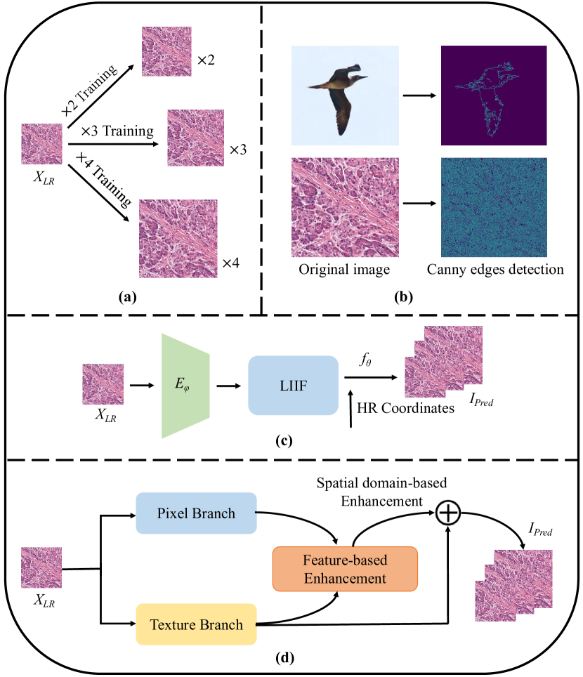
Super-resolution (SR) techniques based on deep learning can accurately map a single low-resolution (LR) image to a high-resolution (HR) image [5, 8, 9], which is an effective way to solve this problem. In pathological image super-resolution, Mukherjee et al. [9] used convolutional neural networks (CNNs) and upsampling layers to generate high-resolution images, and KNN was used to enhance the output results. Li et al. [5] used a U-Net-based generative adversarial network for super-resolution image generation and used curriculum learning as the training strategy. As shown in Figure 1 (a), although these methods achieve good performance, they can only be trained and tested at a fixed integer magnification, and the network needs to be retrained at a specific magnification if other magnifications are needed. However, in clinical pathological diagnosis, doctors usually need to continuously zoom in and out of sections at different magnifications, so the applicability of these models is greatly limited. Unfortunately, to our knowledge, there are currently no models that can achieve arbitrary-scale super-resolution for pathology images.

Recently, inspired by implicit neural networks [11, 10, 12], some studies have pioneered arbitrary-scale super-resolution for natural images. For example, LIIF [13] represents 2D images as latent code through an encoder and maps the input coordinates and corresponding latent variables to RGB values through an MLP-based decoding function, enabling image super-resolution at arbitrary scales. As shown in Figure 1(c), although these methods can be directly applied to pathology images, they do not consider the texture characteristics of pathology images and can only achieve sub-optimal performance. As shown in Figure 1(b), unlike natural images, pathology images contain a large amount of fine-grained cell morphology and repetition. Better reconstructing the special image texture at arbitrary scales is essential in pathology image super-resolution.

In this paper, we propose an efficient two-branch framework based on Implicit Self-Texture Enhancement (ISTE) for arbitrary-scale super-resolution of pathology images to better deal with its special texture. Figure 1(d) briefly illustrates the overall framework of ISTE. Specifically, ISTE contains a pixel learning branch and a texture learning branch, and the two branches are both based on implicit neural networks[13], thus enabling image super-resolution at arbitrary scales. In the pixel learning branch, we propose a Local Feature Interactor module to enhance the perception and interaction of local features and obtain richer pixel features; in the texture learning branch, we propose a Texture Learner module to enhance the network’s learning of texture information. After that, we design a two-stage texture enhancement strategy to fuse the features from the two branches to obtain the super-resolution results, where the first stage is feature-based texture enhancement, and the second stage is spatial domain-based texture enhancement. As shown in Figure 2, considering that pathology images contain many similar cell morphologies and periodic texture patterns, we assume that these similar regions can assist each other in reconstruction in the feature space, so we design the Self-Texture Fusion module to accomplish feature-based texture enhancement. The main idea is to retrieve the texture information most similar to the pixel features for information fusion and enhancement. For spatial domain texture enhancement, we decode the features of the two branches into the spatial domain using Local Pixel Decoder and Local Texture Decoder, respectively, and perform information fusion in the spatial domain. Extensive experiments on three public datasets have shown that ISTE performs better than existing fixed-magnification and arbitrary-magnification algorithms at multiple scales and helps to improve downstream task performance. To the best of our knowledge, this is the first work to achieve arbitrary-scale super-resolution in the field of pathology images. Overall the contributions of this paper are as follows:

• We propose an efficient dual-branch framework based on Implicit Self-Texture Enhancement (ISTE) for arbitrary-scale super-resolution of pathological images. ISTE recovers the texture details of the image through feature-based texture enhancement and spatial domain-based texture enhancement. To the best of our knowledge, it represents the first attempt to achieve arbitrary magnification super-resolution in pathological images.

• The proposed framework achieves state-of-the-art performance at various scale factors on three public datasets, and we demonstrate the effectiveness of the proposed texture enhancement strategy through a series of ablation experiments.

• The pathology images reconstructed by ISTE are shown to be usable in two downstream WSI analysis tasks, gland segmentation and cancer diagnosis, and the performance of these two tasks can be improved by utilizing the reconstructed high-resolution images.

2 Related work

2.1 Deep Learning-Based Super-Resolution Methods for Natural Images

Image super-resolution is the process of recovering an HR image from an LR image or an LR image sequence, which is a classical low-level computer vision task with a wide range of applications. Neural network technology can achieve accurate mapping from low-resolution images to high-resolution images due to its powerful fitting ability and thus has become the mainstream approach in current SR studies. A lot of deep CNN-based methods have been proposed for natural image SR, such as SRCNN [14], EDSR[8], RDN[16], and RCAN[17]. To further improve the performance of SR, some methods use residual modules[18, 19], densely connected modules[20, 21], and other blocks[22, 23] for the design of the CNNs. Subsequently, a series of attention-based SR methods have emerged, such as Channel Attention[24, 17], Self-Attention (IPT [25] and SwinIR[26], HAT[27]), and non-local attention[28, 29]. However, these methods can only be trained and tested at a fixed integer magnification factor and the networks need to be retrained for new magnification factors.

In recent years, Implicit Neural Representation (INR) has been proposed as a continuous data representation for various tasks in computer vision. INR uses a neural network (usually a coordinate-based MLP) to establish a mapping between coordinates and their signal values, which allows continuous and efficient modeling of 2D image signals. As a pioneering work in arbitrary-scale SR, LIIF[13] utilizes MLP as a local implicit neural expression function, which predicts the RGB values at arbitrary query coordinates by capturing HR image coordinates and the surrounding LR features. LTE[30] further introduces a local texture estimator, which transforms coordinates into Fourier domain information to enhance the representational capacity of its local implicit function. Although these methods can be directly applied to pathology images for continuous magnification, they fail to recover the special textures in pathology images effectively.

2.2 Deep Learning-Based Super-Resolution Methods for Microscopy Image

In recent years, deep learning-based SR techniques have been widely used in microscopy images to improve imaging resolution[31, 32, 33, 34]. In [34], the authors developed a cross-modal SR method for fluorescence microscopy to improve the resolution of wide field-of-view images obtained with low numerical aperture objectives. In [32], a Fourier channel attention network was designed to be applied to different microscopic images under different imaging conditions. In pathology image super-resolution, [35] developed a GAN-based approach by considering pathology image SR and surgical smoke removal tasks at the same time. Mukherjee et al.[9] implemented high-resolution image generation using a CNN and up-sampling layer and augmented the outputs using KNN. SRGAN-ResNeXt[36] uses a generative adversarial network based on aggregated residual transformation to train low and high-resolution image pairs, and the generator network is then implemented to perform super-resolution. SWD-Net accomplishes the SR task through a spatial wavelet two-stream network incorporating Refine Context Fusion (RCF)[37]. Under the supervision of spatial and wavelet loss, SWD-Net can recover high-resolution images with clear structural boundaries. WA-SRGAN[38] generates HR images with finer details and less blurring using residual modules and a self-attention mechanism. Li et al.[5] used a U-Net-based generative adversarial network for super-resolution image generation and introduced a curriculum learning training strategy, and conducted experiments to show that the high-resolution images obtained have clinical value. MMSRNet adds a branch for learning magnification classification to the SR network and improves SR performance through multi-task learning[39]. These studies show the promise of using SR to improve the pathology image resolution in low-resource settings. However, they still have some limitations, e.g., training and testing are usually limited to fixed magnification and the SR results still have room for improvement, which we believe is mainly because they do not effectively consider the special texture of pathology images. In this paper, we propose ISTE to address these problems to achieve high-quality arbitrary-scale SR of pathology images.

3 Method

3.1 Problem Formulation and Framework Overview

Given a set of $N$ pairs of corresponding low and high-resolution images ${\left\{X_{LR}^{i},Y_{HR}^{i}\right\}_{i=1}^{N}}$, where ${X_{LR}^{i}}$ is a low-resolution image and ${Y_{HR}^{i}}$ is its corresponding ground truth high-resolution image, the objective is to find the optimal parameters ${\hat{\theta}}$ of the image super-resolution model ${F_{\theta}}$:

$$\hat{\theta}=\arg_{\theta}\min\frac{1}{N}\sum_{i=1}^{N}L\left(F_{\theta}\left(X_{LR}^{i}\right),Y_{HR}^{i}\right)$$ (1)

where ${L}$ is the L1 loss function to measure the difference between the ground-truth and the model-reconstructed high-resolution images.

Figure 2 shows the overall framework of our proposed ISTE, which has a two-branch architecture. We first use SwinIR[26] to perform feature pre-extraction on the input low-resolution image ${X_{LR}}$ and then input the pre-extracted feature map ${F_{LR}}$ into the upper pixel learning branch and lower texture learning branch of ISTE, respectively. Both branches are based on implicit neural networks [20], thus enabling arbitrary-scale magnification. In the pixel learning branch, we input the image feature ${F_{LR}}$ into the Local Feature Interactor module to enhance the network’s perception and interaction of local pixel features and obtain a richer pixel feature ${F_{LFI}}$. Meanwhile, in the texture learning branch, we input the image feature ${F_{LR}}$ into the Texture Learner module to enhance the network’s learning of texture information and extract the texture feature ${F_{TL}}$ efficiently. After that, we design a two-stage texture enhancement strategy for these two branches, where the first stage is feature-based texture enhancement, and the second stage is spatial domain-based texture enhancement. In the first stage, considering that the pathology images contain many similar cell morphologies and periodic texture patterns, we hypothesize that these similar regions can assist each other in the reconstruction through the interaction of the feature space, and thus we designed the Self-Texture Fusion (STF) module to accomplish Feature-based Enhancement. In the second stage, the primary purpose is to fully utilize the texture features ${F_{TL}}$ learned by the Texture Learner and decode them into the spatial domain for texture enhancement. Specifically, we decode the ${F_{STF}}$, which is the output of the first stage feature enhancement, through the Local Pixel Decoder to obtain the RGB image ${I_{LPD}}$. Simultaneously, we decode the texture features ${F_{TL}}$ using the Local Texture Decoder into RGB local texture image ${I_{LTD}}$. Subsequently, we perform spatial summation of ${I_{LTD}}$ and ${I_{LPD}}$, obtaining the final reconstructed high-resolution image ${I_{Pred}}$.

In the following sections, we will introduce the Local Feature Interactor module (section 3.2), the Texture Learner module (section 3.3), the Self-Texture Fusion module (section 3.4), and the Local Pixel and Texture Decoder (Section 3.5), respectively.

Figure 2: Workflow of our ISTE. The low-resolution image $X_{LR}$ is input into the encoder to get the pre-extracted feature map $F_{LR}$ first. In the pixel learning branch, we input the image feature $F_{LR}$ into the Local Feature Interactor module to obtain richer pixel feature. In the texture learning branch, we input the image feature $F_{LR}$ into the Texture Learner module to extract the texture feature. Then the feature maps from the two branches are input to the Self-Texture Fusion (STF) module to accomplish Feature-based Enhancement. Finally, the enhanced feature $F_{STF}$ output from the STF module and the texture feature $F_{TL}$ output from the Texture Learner are decoded into RGB values respectively and added up to accomplish spatial domain-based texture enhancement.

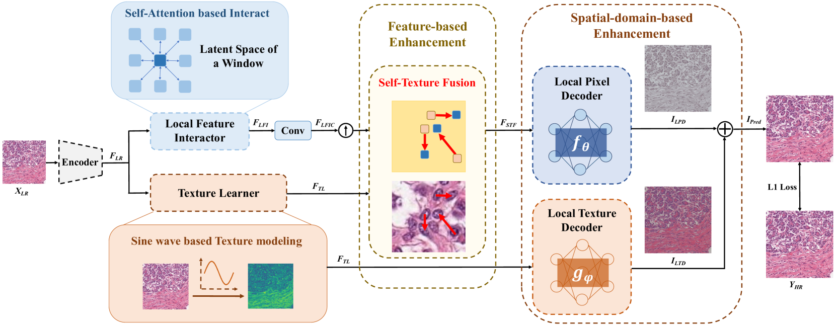
3.2 Local Feature Interactor

As shown in Figure 3, the size of the feature map ${F_{LR}}$ is ${h\times w\times 64}$, and we denote each vector of ${F_{LR}}$ as $F_{LR}^{j}(j=1,2,\ldots,h\times w)$.The Local Feature Interactor (LFI) module first assigns a window of size $3\times 3$ to each vector of ${F_{LR}}$, and the eight neighboring vectors in the window around $F_{LR}^{j}$ form a set $F_{N}^{j}=\left\{F_{N_{i}}^{j}\mid i=3,4,\ldots,10\right\}$. The average pooling result of the vectors within a window is denoted as $F_{P}^{j}$. The feature map ${F_{LFI}}$ output by the LFI module is calculated through self-attention so that each point on the feature map incorporates local features while paying more attention to itself. We denote each vector of ${F_{LFI}}$ as $F_{LFI}^{j}(j=1,2,\ldots,h\times w)$, and it is calculated through equation 2:

$$F_{LFI}^{j}=\sum_{i=1}^{10}\frac{\exp\left(\left(Q_{LR}^{j}\right)^{T}K_{i}^{j}\right)}{\sqrt{d}\sum_{i=1}^{10}\exp\left(\left(Q_{LR}^{j}\right)^{T}K_{i}^{j}\right)}V_{i}^{j}$$ (2)

where $Q_{LR}^{j}$ is the Query mapped linearly from $F_{LR}^{j}$, $K_{1}^{j}$ is the Key mapped linearly from $F_{LR}^{j}$, $V_{1}^{j}$ is the Value mapped linearly from $F_{LR}^{j}$, $K_{2}^{j}$ is the Key mapped linearly from $F_{P}^{j}$, $V_{2}^{j}$ is the Value mapped linearly from $F_{P}^{j}$, $\left\{K_{i}^{j}\mid i=3,4,\ldots,10\right\}$ is the Key mapped linearly from $F_{N}^{j}$, $\left\{V_{i}^{j}\mid i=3,4,\ldots,10\right\}$ is the Value mapped linearly from $F_{N}^{j}$, and $d$ is the dimension of these vectors. The parameters used by each window are shared in the self-attention calculation.

Figure 3: Local Feature Interactor. To enhance the network’s perception of local pixel feature and to obtain richer pixel feature.

Figure 4: (a) Texture Learner (b) Self-Texture Fusion module (c) Coordinate Diagram of $F_{STF}$ and $F_{TL}$ for Local Pixel Decoder and Local Texture Decoder

3.3 Texture Learner

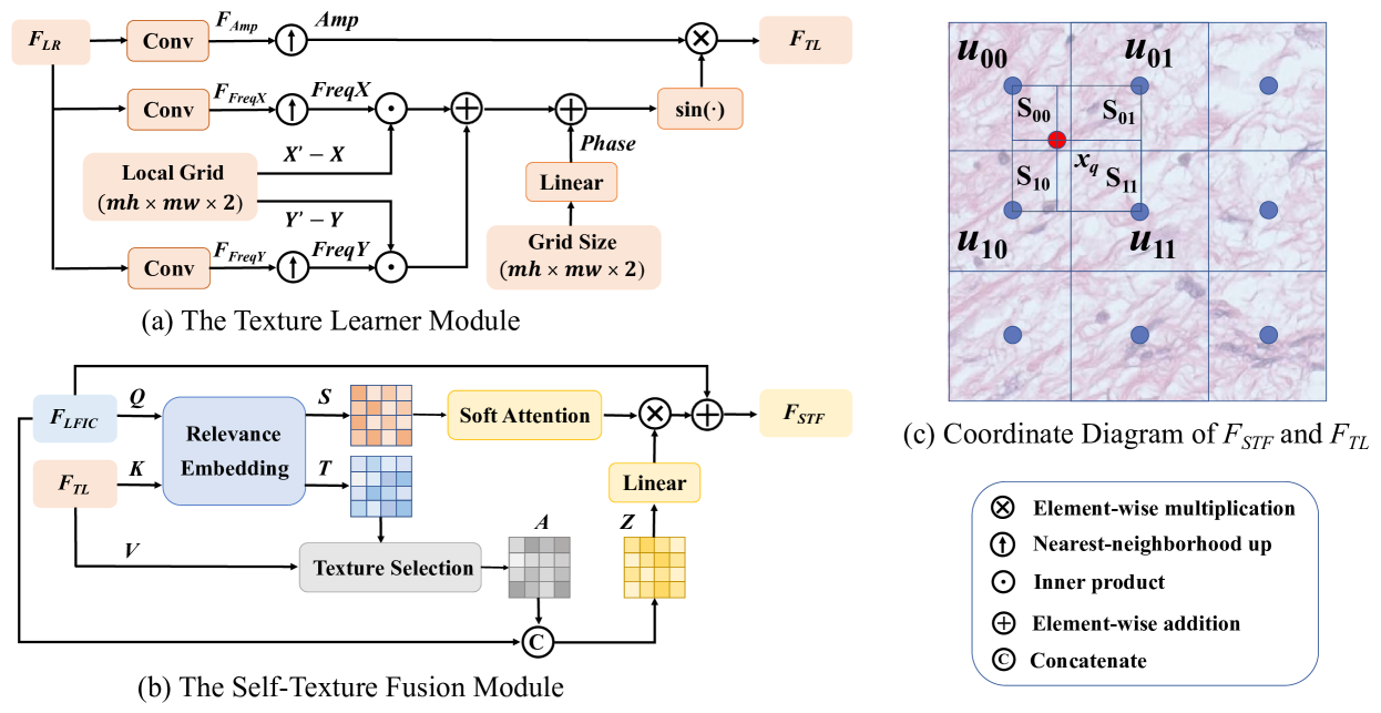
Inspired by [30] and [40], Texture Learner (TL) is proposed for learning texture information in pathology images. We use sine activation to represent the cells and textures that appear periodically in pathology images. Sine functions effectively facilitate implicit neural representation to learn high-frequency details in images, addressing the spectral bias issues arising from ReLU activation functions[12]. Specifically, we normalize the value of 2D pixel coordinate $\left(X^{\prime},Y^{\prime}\right)=\left\{\left(\mathrm{x}_{i}^{\prime},\mathrm{y}_{j}^{\prime}\right)\mid\mathrm{i}=1,2,\ldots,mw,\mathrm{j}=1,2,\ldots,mh\right\}$ in the continuous HR image domain and the value of 2D pixel coordinate $(X,Y)=\left\{\left(\mathrm{x}_{i},\mathrm{y}_{j}\right)\mid\mathrm{i}=1,2,\ldots,mw,\mathrm{j}=1,2,\ldots,mh\right\}$ nearest to $\left(X^{\prime},Y^{\prime}\right)$ in the continuous LR image domain between -1 and 1, and the Local Grid is defined as $\left(X^{\prime}-X,Y^{\prime}-Y\right)$. Since each pixel coordinate of the HR image has a corresponding coordinate in the LR image grid that is closest to it, the number of both the HR and LR image coordinates is equal to $mh\times mw$, where $m$ represents the magnification scale. As shown in Figure 4(a), the TL module firstly outputs three feature maps $F_{Amp}\in h\times w\times 256$, $F_{FreqX}\in h\times w\times 256$ and $F_{FreqY}\in h\times w\times 256$ through three $3\times 3$ convolutional kernels respectively, and predicts the feature maps $Amp\in mh\times mw\times 256$, $FreqX\in mh\times mw\times 256$ and $FreqY\in mh\times mw\times 256$ corresponding to each pixel coordinate of the HR image through nearest-neighbor interpolation. Then we use linear projection based on an MLP and Sigmoid activation function to map $(2/\mathrm{mw},2/\mathrm{mh})$ to a 256-dimensional feature vector $Phase$ to simulate the effect of texture fragment offset when the image scaling factor changes. The output of the TL module is calculated by Equation 3:

$$F_{TL}={Amp}\otimes \operatorname{Sin}({FreqX}\odot\left(X^{\prime}-X\right)+$$ (3)

$${FreqY}\odot\left(Y^{\prime}-Y\right)+{Phase})$$

where $\otimes$ represents element-wise multiplication and $\odot$ represents inner product operation.

3.4 Self-Texture Fusion (STF) Module For Feature-Based Enhancement

Inspired by SRNTT[42] and T2Net[41], we propose a cross-attention-based Self-Texture Fusion (STF) module, whose main idea is to globally retrieve texture features in pixel features and fuse the most similar information weighted to pixel features to accomplish feature-based texture enhancement. As shown in Figure 4(b), we use the features sampled from $F_{LFIC}$ by nearest-neighborhood interpolation as the Query ($Q$) of the cross-attention module and use $F_{TL}$ as the Key ($K$) and Value ($V$) of the cross-attention module. To retrieve the texture features that are most relevant to the pixel feature $F_{LFIC}$, we first compute the similarity matrix $R$ of $Q$ and $K$, where each element $r_{i,j}$ of $R$ is computed according to Equation 4, where $q_{i}$ represents an element of $Q$, and $k_{j}$ represents an element of $K$. Then we obtain the coordinate index matrix $T$ with the highest similarity to $q_{i}$ in $K$. An element in $T$ is $t_{i}=\arg\max_{j}\left(r_{i,j}\right)$, and $t_{i}$ represents the position coordinates of the texture feature $k_{j}$ with the highest similarity to $q_{i}$ in $F_{TL}$. We pick the feature vector $a_{i}$ with the highest similarity to each element in $Q$ from $V$ according to the coordinate index matrix $T$ to obtain the retrieved texture feature $A$, which can be represented by $a_{i}=v_{t_{i}}$ where $a_{i}$ is an element in $A$ and $v_{t_{i}}$ represents the element at the $t_{i}$-th position in $V$. To fuse the retrieved texture feature $A$ with the pixel feature $F_{LFIC}$, we first concatenate $F_{LFIC}$ with $A$ and obtain the aggregated feature $Z$ through the output of an MLP, that is $Z=MLP(Concat(F_{LFIC},A))$. Finally, we calculate the soft attention map $S$, where an element $s_{i}$ in $S$ represents the confidence of each element $a_{i}$ in the retrieved texture feature $A$, and $s_{i}=\max_{j}\left(r_{i,j}\right)$. $F_{STF}$ is calculated as Equation 5:

$$r_{i,j}=\left\langle\frac{q_{i}}{\left\|q_{i}\right\|},\frac{k_{j}}{\left\|k_{j}\right\|}\right\rangle$$ (4)

$$F_{STF}=F_{LFIC}\oplus Z\otimes S$$ (5)

where $\langle\cdot\rangle$ represents inner product operation, $\|\cdot\|$ represents the square root operation, and $\oplus$ represents element-wise summation.

3.5 Spatial Domain-Based Enhancement

In the spatial domain-based texture enhancement, we decode the texture feature $F_{TL}$ directly into the spatial domain $I_{LTD}$ and add it to $I_{LPD}$, which is reconstructed from $F_{FLIC}$ by the Local Pixel Decoder (LPD), to obtain the final output $I_{Pred}$. Firstly, we use the LPD module to decode the feature $F_{STF}$ into the pixel RGB value $I_{LPD}$. We parameterize the LPD module as a multilayer MLP. As shown in Figure 4(c), ${u_{t}}$ denotes the coordinates of the ${F_{LR}}$ and ${x_{q}}$ denotes the coordinates of the ${F_{STF}}$ and $F_{TL}$. We use $u_{t}(t\in 00,01,10,11)$ to denote the upper-left, upper-right, lower-left, and lower-right coordinates of an arbitrary point $x_{q}$, respectively. The RGB value at coordinate ${x_{q}}$ in the HR image decoded by the LPD module can be represented by Equation 6, where $c$ contains two elements, $2/mh$ and $2/mw$, representing the sizes of each pixel in the $I_{LPD}$. Similarly, we compute the RGB values of the texture information $I_{LTD}$ at coordinate $x_{q}$ via Equation 7, where the Local Texture Decoder is parameterized as an MLP $g_{\varphi}$. We use the LTD module to decode the texture features into the spatial domain texture information $I_{LTD}$ and add it to the $I_{LPD}$ via Equation 8 for spatial domain texture enhancement to obtain the prediction result $I_{Pred}$, where ${\varphi}$ is the network parameter of the MLP $g_{\varphi}$. $S_{t}(t\in 00,01,10,11)$ is the area of the rectangular region between $x_{q}$ and $u_{t}$, and the weights are normalized by $S=\sum_{t\in\{00,01,10,11\}}S_{t}$.

$$I_{LPD}=\sum_{t\in\{00,01,10,11\}}\frac{S_{t}}{S}\cdot f_{\theta}\left(F_{STF},x_{q}-u_{t},{c}\right)$$ (6)

$$I_{LTD}=\sum_{t\in\{00,01,10,11\}}\frac{S_{t}}{S}\cdot g_{\varphi}\left(F_{TL}\right)$$ (7)

$$I_{Pred}=I_{LPD}+I_{LTD}$$ (8)

4 Experiments

We first describe the datasets, the implementation details and the results of comparison to SOTA SR methods in section 4.1, 4.2 and 4.3, respectively. Then, we conduct a series of ablation studies in section 4.4. Finally, we perform two downstream task experiments, gland segmentation and cancer diagnosis, to show that the HR images reconstructed by the proposed method can help improve performance on downstream tasks.

4.1 Datasets

4.1.1 TCGA Lung Cancer dataset

The TCGA lung cancer dataset includes 1054 WSIs (average 100000×100000 pixels each)[43] from The Cancer Genome Atlas (TCGA) data center, from which we selected five Slides and cut them into 400 sub-images of 3072×3072 size. We randomly selected 320 sub-images as the training set, 40 as the validation set, and 40 as the test set.

4.1.2 Tissue Microarray (TMA) dataset

Following the work of Li et al.[5], we experimented on the TMA dataset. The TMA dataset, a widely used public dataset in pancreatic cancer research[44, 45], was scanned by an Aperio AT digital pathology scanner (Leica Biosystems, Wetzlar, Germany) at magnification of 0.504 $\upmu$m/pixel and contains 573 WSIs (average 3850×3850 pixels each). We randomly selected 460 WSIs as the training set, 57 WSIs as the validation set, and 56 WSIs as the test set.

4.1.3 Histopathology Super-Resolution (HistoSR) dataset

Following the work of Chen et al.[37], we conducted experiments on the Histopathology Super-Resolution (HistoSR) dataset, which is built on the high-quality H&E stained WSIs of the Camelyon16 dataset. The HistoSR dataset offers High-Resolution (HR) images with a patch size of 192×192 through random cropping and bicubic downsampling. The training set comprises 30000 HR patches, while the test set consists of 5000 HR patches.

4.2 Implementation Details and Evaluation Metrics

Following previous super-resolution methods based on implicit neural representation, we used a ${48\times 48}$ patch as the input for training. We first randomly sampled the magnification m in a uniform distribution U(1, 4) and cropped patches with the size of $48m\times 48m$ from training images in a batch, where ${m}$ represents the magnification scale. We then resized the patches to ${48\times 48}$ and did a Gaussian blur to simulate degradation, and the size of the Gaussian kernel is 1/2 of the magnification scale ${m}$. We sampled $48^{2}$ pixels from the corresponding cropped patches for the ground truth images to form RGB-Coordinate pairs. We use the Pytorch framework to implement the model and use Adam as the optimizer, setting the initial learning rate to 0.0001 and epochs to 1000. Our experimental evaluation indicators include structure similarity index measure (SSIM), peak signal-to-noise ratio (PSNR), and Frechet Inception Distance (FID) for evaluating image perception differences.

Figure 5: Visual comparison with error maps of different methods on the TCGA, TMA, and HistoSR datasets. The error map represents the absolute error value between the output result and the ground truth. The brighter the color, the greater the error.

4.3 Comparison with Previous Methods

We compared the performance of ISTE with SOTA SR methods in both the pathology image domain: SWD-Net[37] and Li et al.[5], and the natural image domain: Bicubic, EDSR[8], SwinIR[26], LIIF[13] and LTE[30], where the latter two are implicit neural network-based methods. For a fair comparison, the backbone used for LIIF and LTE is also SwinIR without upsampling layers.

4.3.1 Quantitative Results

We compared our ISTE with competitors at five magnifications of ×2, ×3, ×4, ×6, and ×8. Table 1 shows the results on the TMA datasets, TCGA datasets, and HistoSR datasets. On the TCGA dataset, ISTE demonstrates the highest performance in terms of PSNR and SSIM metrics across all the magnification levels. Although our method’s FIDs are slightly higher than LIIF by 1.5 at ×8 magnification and slightly higher than SwinIR by 0.21 at ×3 magnification, the FIDs at all other magnifications outperform the comparison methods. On the TMA dataset, our method also achieves the highest performance in terms of PSNR metrics across all the magnification levels. Despite a marginal increase of 0.42 in FID score compared to Li et al.’s method at ×4 magnification level and a slight decrease of 0.0009 in SSIM score compared to LTE at ×8 magnification level, FID and SSIM scores for our method surpass those of the comparison methods at other magnification levels. On the HistoSR dataset, our method achieved the highest performance in terms of PSNR and SSIM metrics at each magnification, but the FID metrics at ×2, ×3, and ×4 are worse than those of Li et al. This is attributed to Li et al.’s incorporation of generative adversarial network techniques to penalize the blurriness in generated images. Additionally, their model was specifically trained at certain magnification levels, resulting in superior performance in terms of image perceptual evaluation compared to our approach.

4.3.2 Qualitative Results

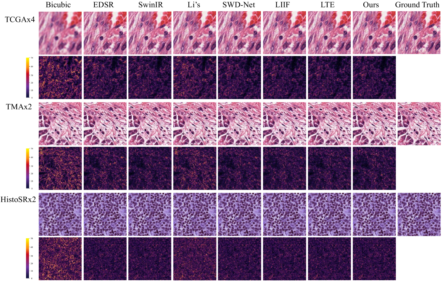
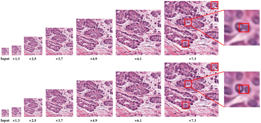
Figure 5 shows the visualization of several examples of super-resolution results and absolute error maps on the TCGA datasets at ×4 magnification, TMA datasets at ×2 magnification, and HistoSR datasets at ×2 magnification. Our proposed method performs better in restoring texture information, closely approximating the ground truth. Based on the brightness levels in the absolute error maps, it is observable that our method’s error maps contain more dark regions, indicating smaller errors in the reconstructed results compared to other methods. Figure 6 shows an example of non-integer magnification of LIIF and our ISTE. It can be seen that ISTE achieves arbitrary magnification with clear cell structure and texture. In larger magnification, ISTE outperforms LIIF in terms of visual effect. As shown in the red box, at the magnification ×7.3, two cells are connected due to blurring in the image generated by LIIF while they are still separated in the image generated by ISTE.

Table 1: Quantitative Results of The Proposed Method ISTE Compared to State-of-the-art Methods on the TCGA, TMA, and HistoSR Datasets

		In-distribution									Out-of-distribution
		×2			×3			×4			×6			×8
Dataset	Methods	PSNR↑	FID↓	SSIM↑	PSNR↑	FID↓	SSIM↑	PSNR↑	FID↓	SSIM↑	PSNR↑	FID↓	SSIM↑	PSNR↑	FID↓	SSIM↑
	Bicubic	32.98	6.96	0.9353	28.12	35.37	0.807	25.63	76.11	0.6874	23.05	129	0.5354	21.64	167.12	0.4606
	EDSR[8]	36.14	1.32	0.9709	31.16	3.43	0.901	28.01	28.2	0.8074	-	-	-	-	-	-
	SwinIR[26]	36.73	1.29	0.9731	31.77	2.65	0.9094	28.83	19.88	0.8258	-	-	-	-	-	-
	Li’s[5]	34.61	2.16	0.958	29.89	4.49	0.8725	26.57	17.16	0.7358	-	-	-	-	-	-
	SWD-Net[37]	36.76	1.23	0.9734	31.73	2.97	0.9074	28.85	17.78	0.8219	-	-	-	-	-	-
	LIIF[13]	36.92	1.23	0.9742	31.99	2.92	0.911	29.08	17.58	0.8275	25.55	88.64	0.6641	23.72	120.62	0.5609
	LTE[30]	36.99	1.22	0.9748	31.98	2.96	0.9109	29.11	17.22	0.828	25.52	90.37	0.6617	23.67	124.3	0.558
TCGA	Ours	37.76	1.07	0.9796	32.06	2.86	0.9124	29.19	16.45	0.8307	25.61	88.62	0.6674	23.76	122.12	0.5637
	Bicubic	28.54	8.58	0.8931	25.25	29.19	0.7708	23.43	54.4	0.6735	21.5	88.33	0.5647	20.44	114.24	0.5123
	EDSR[8]	30.54	3.72	0.937	26.38	11.73	0.8228	24.94	29.07	0.7652	-	-	-	-	-	-
	SwinIR[26]	31.20	3.2	0.9438	28.18	5.57	0.8773	26.26	14.35	0.8092	-	-	-	-	-	-
	Li’s[5]	29.5	4.66	0.9211	26.09	6.53	0.8207	24.06	13.11	0.7206	-	-	-	-	-	-
	SWD-Net[37]	31.18	3.1	0.943	28.06	5.39	0.8746	26.09	15.04	0.8024	-	-	-	-	-	-
	LIIF[13]	30.76	3.63	0.9422	27.84	6.11	0.8745	25.87	17.14	0.799	23.5	53.55	0.6751	22.05	82.5	0.5954
	LTE[30]	31.26	3.15	0.9434	28.19	5.39	0.8784	26.22	15.4	0.8077	23.73	53.66	0.6806	22.17	82.74	0.5974
TMA	Ours	31.27	2.77	0.9444	28.23	4.74	0.8809	26.46	13.53	0.816	23.86	49.27	0.6851	22.19	75.32	0.5965
	Bicubic	27.43	23.6	0.8585	23.88	58.58	0.6999	22.01	93.7	0.577	19.95	172.7	0.4259	18.89	242.28	0.3529
	EDSR[8]	31.53	8.2	0.9407	27.81	37.4	0.8588	25.76	66.03	0.782	-	-	-	-	-	-
	SwinIR[26]	31.51	9.21	0.9397	27.89	38.34	0.8624	25.9	77.72	0.787	-	-	-	-	-	-
	Li’s[5]	28.98	3.86	0.9024	25.34	10.85	0.7843	23.5	17.77	0.6893	-	-	-	-	-	-
	SWD-Net[37]	31.49	8.95	0.9393	27.87	38.92	0.8595	25.78	71.32	0.781	-	-	-	-	-	-
	LIIF[13]	31.56	9.24	0.9399	28.03	39	0.8639	25.93	76.69	0.7862	22.94	130.53	0.6279	20.87	156.85	0.4889
	LTE[30]	31.58	9.54	0.9403	28.03	39.05	0.8647	25.93	77.06	0.7872	22.95	130.56	0.6298	20.89	154.28	0.4909
HistoSR	Ours	31.65	8.92	0.9410	28.14	37.82	0.8673	26.05	75.45	0.7909	23.01	128.81	0.6331	20.94	153.27	0.4948

Table 2: Ablation Study on the TCGA Dataset

	×2			×3			×4
	PSNR↑	FID↓	SSIM↑	PSNR↑	FID↓	SSIM↑	PSNR↑	FID↓	SSIM↑
Ours	37.76	1.07	0.9796	32.06	2.86	0.9124	29.19	16.45	0.8307
w/o LFI	37.61	1.08	0.9788	32.04	2.9	0.9121	29.18	16.69	0.8303
w/o STF	37.66	1.07	0.9791	32.04	2.88	0.9121	29.17	17.05	0.8301
w/o TL	37.64	1.08	0.979	32.04	2.91	0.9121	29.17	16.65	0.8301
w/o LTD	37.63	1.07	0.9789	32.04	2.87	0.912	29.17	16.53	0.8302

Figure 6: Non-integer magnification results of LIIF (upper row) and our ISTE (lower row).

4.4 Ablation Study

To validate the effectiveness of each module in our proposed method, including Local Feature Interactor, Texture Learner, Self-Texture Fusion module, and Texture Decoder module, we designed four variant networks for ablation experiments at magnification factors of ×2, ×3, and ×4 on the TCGA dataset. Moreover, we assessed the efficacy of the Two-Stage texture enhancement strategy proposed in the paper.

4.4.1 Evaluation of Local Feature Interactor

For the features obtained by the encoder $F_{LR}$, the Local Feature Interactor (LFI) module is employed to enhance the network’s perception and interaction with local pixel features, yielding more enriched pixel features $F_{LFI}$. To investigate the effectiveness of the LFI module, we conducted an ablation experiment by directly removing the LFI module from the ISTE framework. As shown in Table 2, all metrics are improved at every magnification by using LFI. Especially, the PSNR is significantly reduced by 0.15, and the SSIM is significantly reduced by 0.0008 at ×2 magnification. At ×3 magnification, The PSNR is significantly reduced by 0.02, and SSIM is significantly reduced by 0.0003.

Figure 7: Feature map visualization for Texture Learner module. $F_{LR}$ represents the feature maps before input to Texture Learner and $F_{TL}$ represents the feature maps output from Texture Learner.

4.4.2 Evaluation of Texture Learner

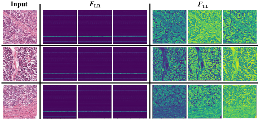
The Texture Learner (TL) module is employed to enhance the network’s learning of high-frequency textures in pathological images, aiming to recover detailed information from LR images better. To investigate the effectiveness of the Texture Learner module, we conducted an ablation experiment by replacing the module with a convolutional layer for network training. As shown in Table 2, it can be seen that after ablating the Texture Learner module, the PSNR metrics were significantly reduced by 0.12 and SSIM by 0.0006 at ×2 magnification. At ×3 magnification, the PSNR metrics were reduced by 0.02 and SSIM by 0.0003. At ×4 magnification, the PSNR metrics were reduced by 0.02 and SSIM by 0.0006. To better illustrate the role of the Texture Learner, we visualized the features before and after the Texture Learner, denoted as $F_{LR}$ and $F_{TL}$, respectively in Figure 7. It is evident that compared to $F_{LR}$, the output feature map $F_{TL}$ from the Texture Learner contains richer texture information. These results confirm the effectiveness of the Texture Learner module in learning texture details.

Figure 8: Visualization of texture similarity retrieval for the STF module, where the blue arrow starting position indicates the position of the texture feature $F_{TL}$ retrieved by the STF module. And the arrow points to the position where the pixel feature $F_{LFIC}$ needs to be enhanced and fused with the retrieved texture feature $F_{TL}$.

4.4.3 Evaluation of Self-Texture Fusion Module

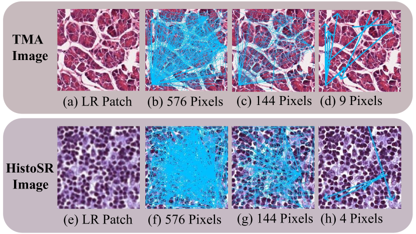
The main role of the Self-Texture Fusion (STF) module is to perform global retrieval in the texture feature $F_{TL}$ and fuse the texture information that is most similar to each position of feature map $F_{FLIC}$ from the pixel branching into the pixel features, thus completing the first stage of feature-based texture enhancement. In order to validate the effectiveness of this module, we designed a variant network without this module. Specifically, first, we take the feature $F_{LFIC}$ obtained from the pixel learning branch of the framework and decode it directly through the Local Pixel Decoder to obtain the Spatial-domain pixel information $I_{LPD}^{\prime}$. Then we take the feature $F_{TL}$ obtained from the texture learning branch and decode it through the Local Texture Decoder to obtain the Spatial-domain texture information $I_{LTD}^{\prime}$. We sum $I_{LPD}^{\prime}$ and $I_{LTD}^{\prime}$ to get the output of the variant network $I_{Pred}^{\prime}$. As shown in Table 2, it can be seen that after ablating the Self-Texture Fusion (STF) module, all metrics become worse at all magnifications. This result confirms the effectiveness of the STF module. To illustrate the effectiveness of the STF module more intuitively, we visualized the path of the STF module to retrieve texture features among the global pixel features on the TMA dataset in Figure 8. For the LR Patch during one training iteration, the starting point of the blue arrow is the position of the texture feature $F_{TL}$ retrieved by the STF module. The arrow points to the position where the pixel feature $F_{LFIC}$ needs to be enhanced and fused with the retrieved texture feature $F_{TL}$. We visualize a proportion of the sampling pixels for a better demonstration in Figure 8. It can be seen that the STF module can effectively use similar tissue texture segments and cellular structure features in pathological images to assist each other’s reconstruction. At the same time, there is a clustering phenomenon at the beginning and ending positions of the texture transfer paths, which indicates that the texture feature at the same position may be fused with the pixel features at several different positions and that the texture feature at several different positions may be fused with the pixel features at the same position. At the same time, the texture features at the same location may be fused with pixel features at multiple different locations.

Figure 9: (a) Input LR image (b) Pixel information decoded by the LPD module (c) Texture information decoded by the LTD module (d) Output of the Spatial Domain-based Enhancement (e) Ground Truth.

4.4.4 Evaluation of Texture Decoder for Spatial Domain-based Enhancement

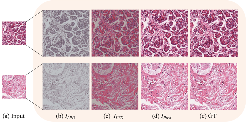
The feature $F_{STF}$ after Feature-based enhancement is decoded into the pixel information $I_{LPD}$ in the spatial domain by the LPD module, and in order to complete the Spatial Domain-based texture enhancement in the second stage, we use the LTD module to decode the texture features learned by Texture Learner directly into the spatial domain texture information $I_{LTD}$ and sum it with $I_{LPD}$ to complete the Spatial Domain-based texture enhancement. In order to demonstrate the effectiveness of the designed Spatial Domain-based Enhancement strategy, we removed the LTD module in the ISTE framework and used only the pixels decoded by the LPD module as the final prediction results. The results in Table 2 suggest that incorporating spatial domain-based texture enhancement on top of feature-based texture enhancement can lead to improved results. To better illustrate the effectiveness of the Spatial Domain-based Enhancement, we visualized the pixel information decoded by the LPD module and the texture information decoded by the LTD in the whole framework of ISTE in Figure 9. It can be seen that the pixel information $I_{LPD}$ decoded only with LPD is relatively smooth and lacks high-frequency texture details, whereas the texture information $I_{LTD}$ decoded with LTD reveals clear outlines and texture features of the tissue cells and has more vibrant colors. This further illustrates the importance of using LTD for the Spatial Domain-based Enhancement.

Table 3: Quantitative evaluation results of U-Net for gland segmentation on the GlaS dataset under different experimental settings.

Experiment	F1		ObjDice		ObjHausdorff
	Test A	Test B	Test A	Test B	Test A	Test B
Bicubic	0.71	0.85	0.83	0.88	133.73	109.21
HR U-Net	0.84	0.88	0.89	0.92	100.57	84.64
SISR	0.92	0.93	0.94	0.95	77.74	65.81
Original high resolution	0.95	0.93	0.96	0.96	66.7	61.17

Figure 10: Quantitative evaluation of UNet for gland segmentation on the GlaS dataset with different experiment setups.

4.5 Downstream Task Experiments

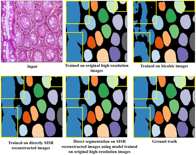
In this section, we experimentally demonstrate that the proposed SR method effectively enhances the performance of two downstream tasks: gland segmentation and cancer classification. First, for the gland segmentation task, we trained and tested the state-of-the-art segmentation model U-Net[47] on the Glas dataset from the MICCAI 2015 Gland Segmentation Challenge[46]. The Glas dataset consists of a training set and two test sets Test A and Test B. The training set contains 85 images and the corresponding labels, Test A contains 60 images and the corresponding labels, and Test B contains 20 images and the corresponding labels. We performed ×4 downsampling on HR images to generate LR images using bicubic interpolation. We compared segmentation results under the following settings: (1) Original High-Resolution: Train U-Net on the original HR GlaS dataset for segmentation of original high-resolution images; (2) SISR: Directly employing U-Net trained on the original HR GlaS dataset for segmentation of the reconstructed images generated by the SISR model. (3) HR U-Net: Train U-Net on the reconstructed images generated by the SISR model for segmentation of original high-resolution images; (4) Bicubic: Train U-Net on LR images obtained after bicubic interpolation for segmentation of original high-resolution images. Table 3 shows the quantitative test results, where larger values indicate better performance for the F1 score and Object Dice score, while smaller values indicate better performance for object Hausdorff distance. It can be seen that the U-Net model trained on the reconstructed images of the SISR model performs significantly better than the U-Net model trained on the LR image dataset after bicubic interpolation, showing higher F1 scores and object Dice scores, as well as lower object Hausdorff distances. In particular, when tested on the Test B dataset, our results for segmentation of reconstructed images using U-Net trained on the original HR GlaS training set are close to those for segmentation of the original high-resolution data, both with an F1 score of 0.93. Figure 10 shows representative results for different experimental setups, and it can be observed that U-Net trained on LR images produced the worst results; not only did it fail to detect small glands, but also the segmentation results of large glands appeared to be significantly crippled. In contrast, the U-Net trained on the reconstructed image could outline the boundaries of the macro glands and detect the tiny glands. Compared to using LR images for network training, using the generated SR images for network training can improve the segmentation accuracy during testing. These results indicate that the method proposed in this paper improves the performance of the segmentation algorithm and can replace the original high-resolution dataset to a certain extent in segmentation tasks, saving data acquisition time and economic costs.

Table 4: The promotion of SR methods on tumor recognition task.

Experiment	Accuracy	F1 score
Original	86.17%	0.8507
Low Resolution	58.11%	0.2929
Bicubic	77.09%	0.7419
LIIF	80.54%	0.7721
ISTE	81.15%	0.7816

To further evaluate the contribution of the SR method to the diagnostic task, we conducted tumor recognition on the PCam dataset[48]. The PCam dataset comprises 262,144 color images for training and 32,768 images for testing, with each image annotated with a binary label indicating the presence of metastatic tissue. We performed ×2 downsampling on HR images of the test set to generate LR images using bicubic interpolation. The ResNet-50[49] was chosen as the classifier and trained on the original PCam dataset. We compared classification results under the following settings: (1) Original: Directly employing the Trained ResNet-50 model to test on the original high-resolution images in the test set; (2) Low Resolution: Directly employing the Trained ResNet-50 model to test on the low-resolution test set images; (3) Bicubic: Directly employing Trained ResNet-50 model to test on the bicubic images of the test set; (4) LIIF: Directly employing Trained ResNet-50 model to test on the images generated by LIIF from the low-resolution test set images; (5) ISTE: Directly employing Trained ResNet-50 model to test on the images generated by our method ISTE from the low-resolution test set images; Table 4 illustrates the enhancement in diagnostic performance by the SR method. By introducing additional prior knowledge, the SR method achieves gains over Bicubic. Clearly, our ISTE leads to a performance improvement, with an accuracy increase of 4.06% compared to Bicubic. These results indicate that ISTE can improve classification performance by recovering more distinctive details.

5 Conclusion

In this work, we propose an innovative two-branch framework ISTE based on self-texture enhancement, which achieves super-resolution of pathology images at arbitrary magnification for the first time. ISTE consists of a pixel-learning branch and a texture-learning branch, where the two branches first learn the pixel features and the texture features, respectively, and then complete feature-based texture enhancement and Spatial domain-based texture enhancement, respectively. Extensive experiments on three publicly available datasets show that ISTE performs better than currently available fixed-magnification and arbitrary-magnification algorithms at multiple magnifications. Further experiments show that our method can improve the performance of two downstream tasks. It is expected that this study will help to increase the penetration of histopathology screening in remote and poor areas that lack high-end imaging equipment. In the future, we will continue to work on lightweight models and integrate the proposed SR models with existing diagnostic networks to improve diagnostic performance.

6 References

References

- [1] J. R. Gilbertson, J. Ho, L. Anthony, D. M. Jukic, Y. Yagi, and A. V. Parwani, “Primary histologic diagnosis using automated whole slide imaging: a validation study,” BMC clinical pathology, vol. 6, pp. 1–19, 2006.
- [2] L. Pantanowitz, P. N. Valenstein, A. J. Evans, K. J. Kaplan, J. D. Pfeifer, D. C. Wilbur, L. C. Collins, and T. J. Colgan, “Review of the current state of whole slide imaging in pathology,” Journal of pathology informatics, vol. 2, no. 1, p. 36, 2011.
- [3] R. S. Weinstein, M. R. Descour, C. Liang, G. Barker, K. M. Scott, L. Richter, E. A. Krupinski, A. K. Bhattacharyya, J. R. Davis, A. R. Graham et al., “An array microscope for ultrarapid virtual slide processing and telepathology. design, fabrication, and validation study,” Human pathology, vol. 35, no. 11, pp. 1303–1314, 2004.
- [4] D. C. Wilbur, “Digital cytology: current state of the art and prospects for the future,” Acta cytologica, vol. 55, no. 3, pp. 227–238, 2011.
- [5] B. Li, A. Keikhosravi, A. G. Loeffler, and K. W. Eliceiri, “Single image super-resolution for whole slide image using convolutional neural networks and self-supervised color normalization,” Medical Image Analysis, vol. 68, p. 101938, 2021.
- [6] L. Pantanowitz, M. Hornish, and R. A. Goulart, “The impact of digital imaging in the field of cytopathology,” Cytojournal, vol. 6, 2009.
- [7] D. C. Wilbur, K. Madi, R. B. Colvin, L. M. Duncan, W. C. Faquin, J. A. Ferry, M. P. Frosch, S. L. Houser, R. L. Kradin, G. Y. Lauwers et al., “Whole-slide imaging digital pathology as a platform for teleconsultation: a pilot study using paired subspecialist correlations,” Archives of pathology & laboratory medicine, vol. 133, no. 12, pp. 1949–1953, 2009.
- [8] B. Lim, S. Son, H. Kim, S. Nah, and K. Mu Lee, “Enhanced deep residual networks for single image super-resolution,” in Proceedings of the IEEE conference on computer vision and pattern recognition workshops, 2017, pp. 136–144.
- [9] L. Mukherjee, A. Keikhosravi, D. Bui, and K. W. Eliceiri, “Convolutional neural networks for whole slide image superresolution,” Biomedical optics express, vol. 9, no. 11, pp. 5368–5386, 2018.
- [10] M. Tancik, P. Srinivasan, B. Mildenhall, S. Fridovich-Keil, N. Raghavan, U. Singhal, R. Ramamoorthi, J. Barron, and R. Ng, “Fourier features let networks learn high frequency functions in low dimensional domains,” Advances in Neural Information Processing Systems, vol. 33, pp. 7537–7547, 2020.
- [11] V. Sitzmann, J. Martel, A. Bergman, D. Lindell, and G. Wetzstein, “Implicit neural representations with periodic activation functions,” Advances in neural information processing systems, vol. 33, pp. 7462–7473, 2020.
- [12] B. Mildenhall, P. P. Srinivasan, M. Tancik, J. T. Barron, R. Ramamoorthi, and R. Ng, “Nerf: Representing scenes as neural radiance fields for view synthesis,” Communications of the ACM, vol. 65, no. 1, pp. 99–106, 2021.
- [13] Y. Chen, S. Liu, and X. Wang, “Learning continuous image representation with local implicit image function,” in Proceedings of the IEEE/CVF conference on computer vision and pattern recognition, 2021, pp. 8628–8638.
- [14] C. Dong, C. C. Loy, K. He, and X. Tang, “Learning a deep convolutional network for image super-resolution,” in Computer Vision–ECCV 2014: 13th European Conference, Zurich, Switzerland, September 6-12, 2014, Proceedings, Part IV 13. Springer, 2014, pp. 184–199.
- [15] C. Ledig, L. Theis, F. Huszár, J. Caballero, A. Cunningham, A. Acosta, A. Aitken, A. Tejani, J. Totz, Z. Wang et al., “Photo-realistic single image super-resolution using a generative adversarial network,” in Proceedings of the IEEE conference on computer vision and pattern recognition, 2017, pp. 4681–4690.
- [16] Y. Zhang, Y. Tian, Y. Kong, B. Zhong, and Y. Fu, “Residual dense network for image super-resolution,” in Proceedings of the IEEE conference on computer vision and pattern recognition, 2018, pp. 2472–2481.
- [17] Y. Zhang, K. Li, K. Li, L. Wang, B. Zhong, and Y. Fu, “Image super-resolution using very deep residual channel attention networks,” in Proceedings of the European conference on computer vision (ECCV), 2018, pp. 286–301.
- [18] L. Cavigelli, P. Hager, and L. Benini, “Cas-cnn: A deep convolutional neural network for image compression artifact suppression,” in 2017 International Joint Conference on Neural Networks (IJCNN). IEEE, 2017, pp. 752–759.
- [19] J. Kim, J. K. Lee, and K. M. Lee, “Accurate image super-resolution using very deep convolutional networks,” in Proceedings of the IEEE conference on computer vision and pattern recognition, 2016, pp. 1646–1654.
- [20] X. Wang, K. Yu, S. Wu, J. Gu, Y. Liu, C. Dong, Y. Qiao, and C. Change Loy, “Esrgan: Enhanced super-resolution generative adversarial networks,” in Proceedings of the European conference on computer vision (ECCV) workshops, 2018, pp. 0–0.
- [21] Y. Zhang, Y. Tian, Y. Kong, B. Zhong, and Y. Fu, “Residual dense network for image restoration,” IEEE transactions on pattern analysis and machine intelligence, vol. 43, no. 7, pp. 2480–2495, 2020.
- [22] Y. Chen and T. Pock, “Trainable nonlinear reaction diffusion: A flexible framework for fast and effective image restoration,” IEEE transactions on pattern analysis and machine intelligence, vol. 39, no. 6, pp. 1256–1272, 2016.
- [23] X. Deng, Y. Zhang, M. Xu, S. Gu, and Y. Duan, “Deep coupled feedback network for joint exposure fusion and image super-resolution,” IEEE Transactions on Image Processing, vol. 30, pp. 3098–3112, 2021.
- [24] B. Niu, W. Wen, W. Ren, X. Zhang, L. Yang, S. Wang, K. Zhang, X. Cao, and H. Shen, “Single image super-resolution via a holistic attention network,” in Computer Vision–ECCV 2020: 16th European Conference, Glasgow, UK, August 23–28, 2020, Proceedings, Part XII 16. Springer, 2020, pp. 191–207.
- [25] H. Chen, Y. Wang, T. Guo, C. Xu, Y. Deng, Z. Liu, S. Ma, C. Xu, C. Xu, and W. Gao, “Pre-trained image processing transformer,” in Proceedings of the IEEE/CVF conference on computer vision and pattern recognition, 2021, pp. 12 299–12 310.
- [26] J. Liang, J. Cao, G. Sun, K. Zhang, L. Van Gool, and R. Timofte, “Swinir: Image restoration using swin transformer,” in Proceedings of the IEEE/CVF international conference on computer vision, 2021, pp. 1833–1844.
- [27] X. Chen, X. Wang, J. Zhou, Y. Qiao, and C. Dong, “Activating more pixels in image super-resolution transformer,” in Proceedings of the IEEE/CVF Conference on Computer Vision and Pattern Recognition, 2023, pp. 22 367–22 377.
- [28] D. Liu, B. Wen, Y. Fan, C. C. Loy, and T. S. Huang, “Non-local recurrent network for image restoration,” Advances in neural information processing systems, vol. 31, 2018.
- [29] Y. Mei, Y. Fan, and Y. Zhou, “Image super-resolution with non-local sparse attention,” in Proceedings of the IEEE/CVF Conference on Computer Vision and Pattern Recognition, 2021, pp. 3517–3526.
- [30] J. Lee and K. H. Jin, “Local texture estimator for implicit representation function,” in Proceedings of the IEEE/CVF conference on computer vision and pattern recognition, 2022, pp. 1929–1938.
- [31] J. Chen, H. Sasaki, H. Lai, Y. Su, J. Liu, Y. Wu, A. Zhovmer, C. A. Combs, I. Rey-Suarez, H.-Y. Chang et al., “Three-dimensional residual channel attention networks denoise and sharpen fluorescence microscopy image volumes,” Nature methods, vol. 18, no. 6, pp. 678–687, 2021.
- [32] C. Qiao, D. Li, Y. Guo, C. Liu, T. Jiang, Q. Dai, and D. Li, “Evaluation and development of deep neural networks for image super-resolution in optical microscopy,” Nature Methods, vol. 18, no. 2, pp. 194–202, 2021.
- [33] M.-S. Kang, E. Cha, E. Kang, J. C. Ye, N.-G. Her, J.-W. Oh, D.-H. Nam, M.-H. Kim, and S. Yang, “Accuracy improvement of quantification information using super-resolution with convolutional neural network for microscopy images,” Biomedical Signal Processing and Control, vol. 58, p. 101846, 2020.
- [34] H. Wang, Y. Rivenson, Y. Jin, Z. Wei, R. Gao, H. Günaydın, L. A. Bentolila, C. Kural, and A. Ozcan, “Deep learning enables cross-modality super-resolution in fluorescence microscopy,” Nature methods, vol. 16, no. 1, pp. 103–110, 2019.
- [35] U. Upadhyay and S. P. Awate, “A mixed-supervision multilevel gan framework for image quality enhancement,” in International Conference on Medical Image Computing and Computer-Assisted Intervention. Springer, 2019, pp. 556–564.
- [36] A. Juhong, B. Li, C.-Y. Yao, C.-W. Yang, D. W. Agnew, Y. L. Lei, X. Huang, W. Piyawattanametha, and Z. Qiu, “Super-resolution and segmentation deep learning for breast cancer histopathology image analysis,” Biomedical Optics Express, vol. 14, no. 1, pp. 18–36, 2023.
- [37] Z. Chen, X. Guo, C. Yang, B. Ibragimov, and Y. Yuan, “Joint spatial-wavelet dual-stream network for super-resolution,” in Medical Image Computing and Computer Assisted Intervention–MICCAI 2020: 23rd International Conference, Lima, Peru, October 4–8, 2020, Proceedings, Part V 23. Springer, 2020, pp. 184–193.
- [38] F. Shahidi, “Breast cancer histopathology image super-resolution using wide-attention gan with improved wasserstein gradient penalty and perceptual loss,” IEEE Access, vol. 9, pp. 32 795–32 809, 2021.
- [39] X. Wu, Z. Chen, C. Peng, and X. Ye, “Mmsrnet: Pathological image super-resolution by multi-task and multi-scale learning,” Biomedical Signal Processing and Control, vol. 81, p. 104428, 2023.
- [40] X. Li, X. Wang, M.-H. Yang, A. A. Efros, and S. Liu, “Scraping textures from natural images for synthesis and editing,” in European Conference on Computer Vision. Springer, 2022, pp. 391–408.
- [41] C.-M. Feng, Y. Yan, H. Fu, L. Chen, and Y. Xu, “Task transformer network for joint mri reconstruction and super-resolution,” in Medical Image Computing and Computer Assisted Intervention–MICCAI 2021: 24th International Conference, Strasbourg, France, September 27–October 1, 2021, Proceedings, Part VI 24. Springer, 2021, pp. 307–317.
- [42] Z. Zhang, Z. Wang, Z. Lin, and H. Qi, “Image super-resolution by neural texture transfer,” in Proceedings of the IEEE/CVF conference on computer vision and pattern recognition, 2019, pp. 7982–7991.
- [43] B. Li, Y. Li, and K. W. Eliceiri, “Dual-stream multiple instance learning network for whole slide image classification with self-supervised contrastive learning,” in Proceedings of the IEEE/CVF conference on computer vision and pattern recognition, 2021, pp. 14 318–14 328.
- [44] C. R. Drifka, A. G. Loeffler, K. Mathewson, A. Keikhosravi, J. C. Eickhoff, Y. Liu, S. M. Weber, W. J. Kao, and K. W. Eliceiri, “Highly aligned stromal collagen is a negative prognostic factor following pancreatic ductal adenocarcinoma resection,” Oncotarget, vol. 7, no. 46, p. 76197, 2016.
- [45] C. R. Drifka, J. Tod, A. G. Loeffler, Y. Liu, G. J. Thomas, K. W. Eliceiri, and W. J. Kao, “Periductal stromal collagen topology of pancreatic ductal adenocarcinoma differs from that of normal and chronic pancreatitis,” Modern Pathology, vol. 28, no. 11, pp. 1470–1480, 2015.
- [46] K. Sirinukunwattana, J. P. Pluim, H. Chen, X. Qi, P.-A. Heng, Y. B. Guo, L. Y. Wang, B. J. Matuszewski, E. Bruni, U. Sanchez et al., “Gland segmentation in colon histology images: The glas challenge contest,” Medical image analysis, vol. 35, pp. 489–502, 2017.
- [47] O. Ronneberger, P. Fischer, and T. Brox, “U-net: Convolutional networks for biomedical image segmentation,” in Medical Image Computing and Computer-Assisted Intervention–MICCAI 2015: 18th International Conference, Munich, Germany, October 5-9, 2015, Proceedings, Part III 18. Springer, 2015, pp. 234–241.
- [48] B. S. Veeling, J. Linmans, J. Winkens, T. Cohen, and M. Welling, “Rotation equivariant cnns for digital pathology,” in Medical Image Computing and Computer Assisted Intervention–MICCAI 2018: 21st International Conference, Granada, Spain, September 16-20, 2018, Proceedings, Part II 11. Springer, 2018, pp. 210–218.
- [49] K. He, X. Zhang, S. Ren, and J. Sun, “Deep residual learning for image recognition,” in Proceedings of the IEEE conference on computer vision and pattern recognition, 2016, pp. 770–778.