Analysis for a class of stochastic fractional nonlinear Schrödinger equations

Abstract

We investigate the global existence of a solution for the stochastic fractional nonlinear Schrödinger equation with radially symmetric initial data in a suitable energy space $H^{\alpha}$. Using a variational principle, we demonstrate that the stochastic fractional nonlinear Schrödinger equation in the Stratonovich sense forms an infinite-dimensional stochastic Hamiltonian system, with its phase flow preserving symplecticity. We develop a structure-preserving algorithm for the stochastic fractional nonlinear Schrödinger equation from the perspective of symplectic geometry. It is established that the stochastic midpoint scheme satisfies the corresponding symplectic law in the discrete sense. Furthermore, since the midpoint scheme is implicit, we also develop a more effective mass-preserving splitting scheme. Consequently, the convergence order of the splitting scheme is shown to be $1$. Two numerical examples are conducted to validate the efficiency of the theory.

1 Introduction.

The fractional nonlinear Schrödinger equation, as an extension of the standard Schrödinger equation, arises in diverse fields like nonlinear optics [1], quantum physics [2], and water propagation [3]. Inspired by the Feynman path approach to quantum mechanics, Laskin [4] utilized the path integral over Lévy-like quantum mechanical paths to derive a fractional Schrödinger equation. Kirkpatrick [5] examined a broad range of discrete nonlinear Schrödinger equations on the lattice $h\mathbb{Z}$ with mesh size $h>0$. They demonstrated that the resulting dynamics converge to a nonlinear fractional Schrödinger equation as $h\rightarrow 0$. Ionescu and Pusateri [6] demonstrated the global existence of small, smooth, and localized solutions for a specific fractional semilinear cubic nonlinear Schrödinger equation in one dimension. Shang and Zhang [7] investigated the existence and multiplicity of solutions for the critical fractional Schrödinger equation. They demonstrated the presence of a nonnegative ground state solution and explored the relationship between the number of solutions and the topology of the set. Choi and Aceves [8] proved that the solutions to the discrete nonlinear Schrödinger equation with non-local algebraically decaying coupling converged strongly in $L^{2}(\mathbb{R}^{n})$ to those of the continuum fractional nonlinear Schrödinger equation. Frank and his colleagues [9] established general uniqueness findings for radial solutions of linear and nonlinear equations involving the fractional Laplacian $(-\Delta)^{\alpha}$ with $\alpha\in(0,1)$ for any space dimensions $n\geq 1$. Wang and Huang [10] presented an energy-conserving difference scheme for the nonlinear fractional Schrödinger equations and provided a thorough analysis of the conservation property. Duo and Zhang [11] proposed three mass-conservative Fourier spectral methods for solving the fractional nonlinear Schrödinger equation.

In certain situations, it is necessary to consider randomness. Understanding the impact of noise on wave propagation is a major challenge, as it can significantly alter the qualitative behavior and lead to new properties. Stochastic nonlinear Schrödinger equations are employed as nonlocal models for wave propagation in various physical applications. For the stochastic Schrödinger equation driven by Gaussian noise, Bouard and Debussche [12, 13] examined a conservative stochastic nonlinear Schrödinger equation and the impact of multiplicative Gaussian noises, demonstrating the global presence and uniqueness of solutions. Herr et al. [14] examined the scattering behavior of global solutions to stochastic nonlinear Schrödinger equations with linear multiplicative noise. Barue et al. [15] demonstrated that the explosion could be effectively prevented over the entire time interval $[0,\infty)$. Deng et al. [16] researched the spread of randomness in nonlinear dispersive equations using the theory of random tensors. Bouard and Debusschev [17, 18] developed a semi-discrete method for numerically approximating the stochastic nonlinear Schrödinger equation in the Stratonovich sense. Cui and his colleagues [19] gave the strong convergence rate of the splitting scheme for stochastic Schrödinger equations. Liu [20, 21] examined the error of a semi-discrete method and demonstrated that the numerical scheme possessed a strong order of $\frac{1}{2}$. Chen and Hong [22] introduced a broad category of stochastic symplectic Runge-Kutta methods for the temporal direction of the stochastic Schrödinger equation in the Stratonovich sense. Anton and Cohen [23] demonstrated the robust convergence of an exponential integrator for the time discretization of stochastic Schrödinger equations influenced by additive or multiplicative Itô noise. Cui et al. [24, 25, 26] introduced the stochastic symplectic and multi-symplectic methods and demonstrated their convergence with a temporal order of one in probability. They also proved a strong rate $1/2$ as well as a weak rate $1$ of a splitting scheme for a damped stochastic cubic Schrödinger equation with linear multiplicative trace-class noise and large enough damping term. Bréhier and Cohen [27] investigated the qualitative characteristics and convergence order of a splitting scheme for the stochastic Schrödinger equations with additive noise. They showed the stochastic symplecticity of the numerical solution and consistently preserved the expected mass. Yang and Chen [28] demonstrated the presence of martingale solutions for the stochastic fractional nonlinear Schrödinger equation on a limited interval. Zhang et al. [29] proved the existence and uniqueness of a global solution to the stochastic fractional nonlinear Schrödinger equation in $L^{2}(\mathbb{R}^{n})$. For the stochastic Schrödinger equation driven by jump noise, Liu and his collaborators [30] established a new version of the stochastic Strichartz estimate for the stochastic convolution driven by jump noise. Wang et al. [31] also established the existence and uniqueness of solutions of stochastic nonlinear Schrödinger equations with additive jump noise in $L^{2}(\mathbb{R}^{d})$. There is limited research on the well-posedness of the solution in the energy space $H^{\alpha}$, its stochastic symplectic and convergence theorem, and symplectic semi-discretization for stochastic fractional nonlinear Schrödinger equation with multiplicative noise.

This paper focuses on the examination of the stochastic fractional nonlinear Schrödinger equation (SFNSE) with multiplicative noise in $H^{\alpha}(\mathbb{R}^{n})$, i.e.,

$$\left\{\begin{aligned} &idu-\left[(-\Delta)^{\alpha}u+\lambda|u|^{2\sigma}u\right]dt=u\circ dW(t),\quad x\in\mathbb{R}^{n},\quad t\geq 0,\\ &u(0)=u_{0},\end{aligned}\right.$$ (1.1)

where $u$ is a complex-valued process defined on $\mathbb{R}^{+}\times\mathbb{R}^{n}$, $0<\sigma<\infty$, and $W(t)$ is a Wiener process. The parameter $\lambda=1$ (resp. $\lambda=-1$) corresponds to the defocusing (resp. focusing) case. The fractional Laplacian operator $(-\Delta)^{\alpha}$ with an admissible exponent $\alpha\in(\frac{1}{2},1)$ is involved. The notation $\circ$ stands for the Stratonovitch integral.

Consider a probability space $(\Omega,\mathcal{F},\mathbb{P})$, a filtration $\left(\mathcal{F}_{t}\right)_{t\geq 0}$, and a sequence of independent Brownian motions $\left(\beta_{k}\right)_{k\in\mathbb{N}^{+}}$ associated with this filtration. Given $\left(e_{k}\right)_{k\in\mathbb{N}^{+}}$ an orthonormal basis of $L^{2}\left(\mathbb{R}^{n},\mathbb{R}\right)$, and a linear operator $\Phi$ on $L^{2}\left(\mathbb{R}^{n},\mathbb{R}\right)$ with a real-valued kernel $k$:

$$\Phi h(x)=\int_{\mathbb{R}^{n}}k(x,y)h(y)dy,\quad h\in L^{2}\left(\mathbb{R}^{n},\mathbb{R}\right).$$ (1.2)

Then the process

$$W(t,x,\omega):=\sum_{k=1}^{\infty}\beta_{k}(t,\omega)\Phi e_{k}(x),\quad t\geq 0,\quad x\in\mathbb{R}^{n},\quad\omega\in\Omega,$$

is a Wiener process on $L^{2}\left(\mathbb{R}^{n},\mathbb{R}\right)$ with covariance operator $\Phi\Phi^{*}$, and the equation (1.1) can be rewritten as

$$idu-\left[(-\Delta)^{\alpha}u+\lambda|u|^{2\sigma}u\right]dt=udW-\frac{1}{2}iuF_{\Phi}dt,$$ (1.3)

where the function $F_{\Phi}$ is given by

$$F_{\Phi}(x)=\sum_{k=1}^{\infty}\left(\Phi e_{k}(x)\right)^{2},\quad x\in\mathbb{R}^{n}.$$ (1.4)

We are interested in the global existence and uniqueness of the solution, its stochastic symplecticity, and the convergence theorem for the stochastic fractional nonlinear Schrödinger equation. We seek to address the following unlike existing results:

1. Global existence of a solution for the stochastic fractional nonlinear Schrödinger equation with radially symmetric initial data in the energy space $H^{\alpha}$.

2. The stochastic fractional nonlinear Schrödinger equation in the Stratonovich sense is an infinite-dimensional stochastic Hamiltonian system.

3. Preservation of symplecticity for the exact solution.

4. Construction of the stochastic multi-symplectic method in the discrete case.

5. Convergence estimates of the splitting scheme and order of convergence.

In Section 2, we introduce notations for the coefficients required by our main result. Section 3 is dedicated to the existence of a global solution of equation (1.1) in the energy space $H^{\alpha}$. In Section 4, we demonstrate that the stochastic fractional nonlinear Schrödinger equation is an infinite-dimensional Hamiltonian system, analyze its stochastic multi-symplectic structure, and develop a structure-preserving algorithm for the stochastic fractional nonlinear Schrödinger equation from the perspective of symplectic geometry. Section 5 focuses on constructing a more effective mass-preserving splitting scheme for the stochastic fractional nonlinear Schrödinger equation in the Stratonovich sense, and provides the rate of convergence of a splitting scheme. Two numerical tests are conducted to validate the efficiency in Section 4 and Section 5, respectively.

2 Preliminaries

Throughout this paper, we use some notations. The capital letter $C$ represents a positive constant, with its value possibly changing from one line to the next. The notation $C_{p}$ is specifically used to indicate that the constant depends on the parameter $p$. For $p\geq 2$, $L^{p}$ denotes the Lebesgue space of complex-valued functions. The inner product in $L^{2}\left(\mathbb{R}^{n}\right)$ is defined as

$$(f,g)={\bf{Re}}\int_{\mathbb{R}^{n}}f(x)\bar{g}(x)dx,\quad\text{for}~{}~{}f,g\in L^{2}\left(\mathbb{R}^{n}\right).$$

Given a Banach space $B$, we denote by $R(H;B)$ the $\gamma$-radonifying operator from $H$ into $B$ [38], equipped with the norm

$$\|K\|^{2}_{R(H,B)}=\widetilde{\mathbb{E}}\left|\sum_{k=1}^{\infty}\gamma_{k}Ke_{k}\right|^{2}_{B},$$

where $(e_{k})_{k\in\mathbb{N}}$ is any orthonormal basis of $H$, and $(\gamma_{k})_{k\in\mathbb{N}}$ is any sequence of independent normal real-valued random variables on a probability space $\left(\widetilde{\Omega},\widetilde{\mathcal{F}},\widetilde{P}\right)$. $\widetilde{E}$ is the expectation on $\left(\widetilde{\Omega},\widetilde{\mathcal{F}},\widetilde{P}\right)$.

We define the standard space $H^{\alpha}\left(\mathbb{R}^{n}\right)$ for tempered distributions $u\in$ $\mathcal{S}^{\prime}\left(\mathbb{R}^{n}\right)$ with Fourier transform $\hat{u}$ satisfying $\left(1+|\xi|^{2}\right)^{{\alpha}/2}\hat{u}\in L^{2}\left(\mathbb{R}^{n}\right)$. We may use the abbreviated notation $L^{r}\left(0,T;L_{x}^{p}\right)$ for $L^{r}\left([0,T];L^{p}\left(\mathbb{R}^{n}\right)\right)$, or even $L_{t}^{r}\left(L_{x}^{p}\right)$ when the interval $[0,T]$ is specified and fixed. Given two separable Hilbert spaces $H$ and $\widetilde{H}$, the notation $L_{HS}(H,\widetilde{H})$ denotes the space of Hilbert-Schmidt operators from $H$ into $\widetilde{H}$. Let $\Phi:H\rightarrow\widetilde{H}$ be a bounded linear operator. The operator $\Phi$ is called the Hilbert-Schmidt operator if there is an orthonormal basis $(e_{k})_{k\in\mathbb{N}^{+}}$ in $H$ such that

$$\|\Phi\|^{2}_{L_{HS}(H,\widetilde{H})}=\operatorname{tr}\Phi^{*}\Phi=\sum_{k=1}^{\infty}\left|\Phi e_{k}\right|_{\widetilde{H}}^{2}<\infty.$$

When $H=\widetilde{H}=L^{2}(\mathbb{R}^{n};\mathbb{R})$, $L_{HS}\left(L^{2}(\mathbb{R}^{n};\mathbb{R}),L^{2}(\mathbb{R}^{n};\mathbb{R})\right)$ is simply denoted by $L_{HS}$. Note that if $K$ is a Hilbert space such that $K\subset E$ with a continuous embedding then $L_{HS}(H,K)\subset R(H,E)$ with a continuous embedding.

We also use $\nabla$ to denote the gradient operator in Euclidean space. Let $L(E;F)$ denote the space of bounded linear operators from $E$ into $F$. Let $(m,p)$ be in $\mathbb{N}\times[1,\infty)$. The Banach space $W^{m,p}(\mathbb{R}^{n})$ consists of measurable functions $u$ on $\mathbb{R}^{n}$ such that $\nabla^{\beta}u\in L^{p}(\mathbb{R}^{n})$ in the sense of distributions, for every multi-index $\beta$ with $|\beta|\leq m$. $W^{m,p}(\mathbb{R}^{n})$ is equipped with the norm

$$\|u\|_{W^{m,p}}=\sum_{|\beta|\leq m}\|\nabla^{\beta}u\|_{L^{p}}.$$

The space $\mathcal{C}^{1,1}_{loc}\cap\mathcal{L}_{\alpha}$ consists of measurable functions $u$ on $\mathbb{R}^{n}$ such that $u\in L^{1}_{loc}$ and $\int_{\mathbb{R}^{n}}\frac{|u(x)|}{1+|x|^{n+2\alpha}}dx<\infty$.

In the following, we present criteria for determining if a stochastic system is a stochastic Hamiltonian system, which comes from [32, 33].

Definition 1.

For the $2n$-dimensional stochastic differential equation in Stratonovich sense

$$\left\{\begin{aligned} dp&=f(t,p,q)dt+\sum_{k=1}^{r}\sigma_{k}(t,p,q)\circ dW_{k}(t),~{}~{}p(t_{0})=p_{0},\\ dq&=g(t,p,q)dt+\sum_{k=1}^{r}\gamma_{k}(t,p,q)\circ dW_{k}(t),~{}~{}q(t_{0})=q_{0},\\ \end{aligned}\right.$$ (2.1)

if there are functions $H(t,p,q)$ and $H_{k}(t,p,q)(k=1,2,\cdots,r)$ such that

$$f(t,p,q) =-\frac{\partial H(t,p,q)}{\partial q}^{T},~{}~{}~{}\sigma_{k}(t,p,q)=-\frac{\partial\widetilde{H}_{k}(t,p,q)}{\partial q}^{T},$$ (2.2)

$$g(t,p,q) =\frac{\partial H(t,p,q)}{\partial p}^{T},~{}~{}~{}\gamma_{k}(t,p,q)=\frac{\partial\widetilde{H}_{k}(t,p,q)}{\partial p}^{T},$$

for $k=1,\cdots,r$, then it is a stochastic Hamiltonian system.

Here, we will discuss fractional derivatives [34]. The fractional Laplace $(-\Delta)^{\alpha}$ is defined as

$$(-\Delta)^{\alpha}u(x)=C(n,\alpha)~{}\mathrm{P.V.}\int_{\mathbb{R}^{n}}\frac{u(x)-u(y)}{|x-y|^{n+2\alpha}}dy,\\$$

where $\mathrm{P.V.}$ denotes the principal value of the integral, and $C(n,\alpha)$ is a positive constant given by

$$C(n,\alpha)=\frac{2^{2\alpha}\alpha\Gamma(\frac{n+2\alpha}{2})}{\pi^{\frac{n}{2}}\Gamma(1-\alpha)}.$$

For every $\alpha\in(0,1)$, denote by

$$H^{\alpha}(\mathbb{R}^{n}):=\left\{u\in L^{2}(\mathbb{R}^{n}):\int_{\mathbb{R}^{n}}\int_{\mathbb{R}^{n}}\frac{|u(x)-u(y)|^{2}}{|x-y|^{n+2\alpha}}dxdy<\infty\right\}.$$

Then $H^{\alpha}(\mathbb{R}^{n})$ is a Hilbert space with inner product given by

$$(u,v)_{H^{\alpha}(\mathbb{R}^{n})}=(u,v)_{L^{2}(\mathbb{R}^{n})}+\mathbf{Re}\int_{\mathbb{R}^{n}}\int_{\mathbb{R}^{n}}\frac{\left(u(x)-u(y)\right)\left(\bar{v}(x)-\bar{v}(y)\right)}{|x-y|^{n+2\alpha}}dxdy,\quad u,v\in H^{\alpha}(\mathbb{R}^{n}).$$

In the following, we will also give the notation

$$(u,v)_{\dot{H}^{\alpha}(\mathbb{R}^{n})}=\mathbf{Re}\int_{\mathbb{R}^{n}}\int_{\mathbb{R}^{n}}\frac{\left(u(x)-u(y)\right)\left(\bar{v}(x)-\bar{v}(y)\right)}{|x-y|^{n+2\alpha}}dxdy,\quad u,v\in H^{\alpha}(\mathbb{R}^{n}),$$

and

$$\|u\|^{2}_{\dot{H}^{\alpha}(\mathbb{R}^{n})}=\int_{\mathbb{R}^{n}}\int_{\mathbb{R}^{n}}\frac{\left|u(x)-u(y)\right|^{2}}{|x-y|^{n+2\alpha}}dxdy,\quad u\in H^{\alpha}(\mathbb{R}^{n}).$$

Then we have

$$(u,v)_{H^{\alpha}(\mathbb{R}^{n})}=(u,v)_{L^{2}(\mathbb{R}^{n})}+(u,v)_{\dot{H}^{\alpha}(\mathbb{R}^{n})},\quad u,v\in H^{\alpha}(\mathbb{R}^{n}),$$

and

$$\|u\|^{2}_{H^{\alpha}(\mathbb{R}^{n})}=\|u\|^{2}_{L^{2}(\mathbb{R}^{n})}+\|u\|^{2}_{\dot{H}^{\alpha}(\mathbb{R}^{n})},\quad u\in H^{\alpha}(\mathbb{R}^{n}).$$

By [35], we know that

$$\|(-\Delta)^{\frac{\alpha}{2}}u\|^{2}_{L^{2}(\mathbb{R}^{n})}=\frac{1}{2}C(n,\alpha)\|u\|^{2}_{\dot{H}^{\alpha}(\mathbb{R}^{n})},$$

and the norm $\|u\|_{H^{\alpha}\left(\mathbb{R}^{n}\right)}$ is equivalent to the norm $\left(\|u\|_{L^{2}\left(\mathbb{R}^{n}\right)}^{2}+\left\|(-\Delta)^{\frac{\alpha}{2}}u\right\|_{L^{2}\left(\mathbb{R}^{n}\right)}^{2}\right)^{\frac{1}{2}}$ for any $u\in H^{\alpha}\left(\mathbb{R}^{n}\right)$.

3 Global Existence

This section focuses on studying the global existence of the stochastic fractional nonlinear Schrödinger equation (1.1) with radially symmetric initial data in the energy space $H^{\alpha}$. Let us first recall the definition of an admissible pair. We say a pair $(p,q)$ satisfies the fractional admissible condition if

$$p\in[2,\infty],\quad q\in[2,\infty),\quad(p,q)\neq\left(2,\frac{4n-2}{2n-3}\right),\quad\frac{2\alpha}{p}+\frac{n}{q}=\frac{n}{2}.$$ (3.1)

The unitary group $S(t):=e^{-it(-\Delta)^{\alpha}}$ enjoys several types of Strichartz estimates, for instance, non-radial Strichartz estimates, radial Strichartz estimates, and weighted Strichartz estimates. We only recall here radial Strichartz estimates (see, e.g., Ref. [36]).

Lemma 1.

(Radial Strichartz estimates) For $n\geq 2$ and $\frac{n}{2n-1}\leq\alpha<1$, there exists a positive constant $C$ such that the following estimates hold:

$$\left\|e^{-it(-\Delta)^{\alpha}}\psi\right\|_{L^{p}\left(\mathbb{R},L^{q}\right)} \leq C\|\psi\|_{L^{2}},$$ (3.2)

$$\left\|\int_{0}^{t}S(t-s)f(s)ds\right\|_{L^{p}\left(\mathbb{R},L^{q}\right)} \leq C\|f\|_{L^{\beta^{\prime}}\left(\mathbb{R},L^{\gamma^{\prime}}\right)},$$

where $\psi$ and $f$ are radially symmetric, $(p,q)$ and $(\beta,\gamma)$ satisfy the fractional admissible condition, and $\frac{1}{\beta^{\prime}}+\frac{1}{\beta}=\frac{1}{\gamma^{\prime}}+\frac{1}{\gamma}=1$.

Assumption 1.

(On the noise) We assume that $\Phi:L^{2}\rightarrow H^{\alpha}$ is a Hilbert-Schmidt operator, i.e.

$$\|\Phi\|_{L_{HS}(L^{2},H^{\alpha})}:=\left(\sum_{k=1}^{\infty}\left\|\Phi e_{k}\right\|_{H^{\alpha}}^{2}\right)^{1/2}<\infty.$$

This implies that

$$\|\Phi\|_{L_{HS}(L^{2};H^{\alpha})}^{2}=\sum_{k=1}^{\infty}\left\|\Phi e_{k}\right\|^{2}+\sum_{k=1}^{\infty}\left\|(-\Delta)^{\frac{\alpha}{2}}\Phi e_{k}\right\|^{2}.$$

Assumption 2.

(On the nonlinearity)

1. If $\lambda=-1$ (focusing), let $0\leq\sigma<\frac{2\alpha}{n}$.

2. If $\lambda=1$ (defocusing), let $\begin{cases}0\leq\sigma<\frac{2\alpha}{n-2\alpha},&\text{ for }n\geq 2,\\ \sigma\geq 0,&\text{ for }n<2.\end{cases}$

We recall the following fractional chain rule [37], which is needed in the local well-posedness for (1.1).

Lemma 2.

Let $F\in C^{1}(\mathbb{C},\mathbb{C})$ and $\alpha\in(0,1)$. Then for $1<q\leq q_{2}<\infty$ and $1<q_{1}\leq\infty$ satisfying $\frac{1}{q}=\frac{1}{q_{1}}+\frac{1}{q_{2}}$, there exists a positive constant $C$ such that

$$\left\||\nabla|^{\alpha}F(u)\right\|_{L^{q}}\leq C\left\|F^{\prime}(u)\right\|_{L^{q_{1}}}\left\||\nabla|^{\alpha}u\right\|_{L^{q_{2}}}.$$ (3.3)

The next lemma is a straightforward generalization of Lemma 3.1 and Lemma 3.2 in [12].

Lemma 3.

Assume that a pair $(p,q)$ satisfies the fractional admissible condition, $q<\frac{2n}{n-\alpha}$, $T_{0}>0$, and take $\rho\geq p$. Under Assumption 1, for any $u$ radially adapted process in $L^{\rho}\left(\Omega;L^{p}\left(0,T_{0};W^{\alpha,q}\right)\right)\cap L^{\rho}\left(\Omega;L^{\infty}\left(0,T_{0};H^{\alpha}\right)\right)$ if $Iu$ is defined for $t_{0},t\in\left[0,T_{0}\right]$ by

$$Iu\left(t_{0},t\right)=\int_{0}^{t_{0}}S(t-s)(u(s)dW(s)),$$

Then for any stopping time $\tau$ with $\tau<T_{0}$ almost surely,

$$\mathbb{E}\left(\sup_{0\leq t_{0}\leq\tau}\left|Iu\left(t_{0},\cdot\right)\right|_{L^{p}\left(0,\tau;W^{\alpha,q}\right)}^{\rho}\right)\leq C\left(\rho,T_{0},\|\Phi\|_{L_{HS}(L^{2},H^{\alpha})}\right)T_{0}^{\delta}\mathbb{E}\left(|u|_{L^{\infty}\left(0,\tau;H^{\alpha}\right)}^{\rho}\right)$$

with $\delta>0$. Furthermore, if we set $Ju(t)=Iu(t,t)$ then $Ju$ has a modification in $L^{\rho}\left(\Omega;L^{p}\left(0,T_{0};W^{\alpha,q}\right)\cap C\left(\left[0,T_{0}\right];H^{\alpha}\right)\right)$ and

$$\mathbb{E}\left(|Ju|_{L^{p}\left(0,\tau;W^{\alpha,q}\right)}^{\rho}\right)\leq C\left(\rho,T_{0},\|\Phi\|_{L_{HS}(L^{2},H^{\alpha})}\right)T_{0}^{\delta}\mathbb{E}\left(|u|_{L^{\infty}\left(0,\tau;H^{\alpha}\right)}^{\rho}\right)$$

and

$$\mathbb{E}\left(\sup_{0\leq t\leq\tau}|Ju(t)|_{H^{\alpha}}^{\rho}\right)\leq C\left(\rho,T_{0},\|\Phi\|_{L_{HS}(L^{2},H^{\alpha})}\right)T_{0}^{\delta}\mathbb{E}\left(|u|_{L^{p}\left(0,\tau;W^{\alpha,q}\right)}^{\rho}\right).$$

Next, we give the local well-posedness of the stochastic fractional nonlinear Schrödinger equation (1.1) with radially symmetric initial data in the energy space $H^{\alpha}$.

Theorem 1.

(Radial local theory). Let $n\geq 2$ and $\alpha\in\left[\frac{n}{2n-1},1\right)$ and $0<\sigma<\frac{2\alpha}{n-2\alpha}$. Let

$$p=\frac{4\alpha(\sigma+2)}{\sigma(n-2\alpha)},\quad q=\frac{n(\sigma+2)}{n+\sigma\alpha}.$$

Then under Assumption 1, for any $u_{0}\in H^{\alpha}$ radial, there exists a stopping time $\tau^{*}\left(u_{0},\omega\right)$ and a unique solution to (1.1) starting from $u_{0}$, which is almost surely in $C\left([0,\tau];H^{\alpha}\right)\cap L^{p}\left(0,\tau;W^{\alpha,q}\right)$ for any $\tau<\tau^{*}\left(u_{0}\right)$. Moreover, we have almost surely,

$$\tau^{*}\left(u_{0},\omega\right)=+\infty\quad\text{ or }\quad\limsup_{t\to\tau^{*}\left(u_{0},\omega\right)}|u(t)|_{H^{\alpha}}=+\infty.$$

Proof.

It is easy to check that $(p,q)$ satisfies the fractional admissible condition. We choose $(a,b)$ so that

$$\frac{1}{p^{\prime}}=\frac{1}{p}+\frac{2\sigma}{a},\quad\frac{1}{q^{\prime}}=\frac{1}{q}+\frac{2\sigma}{b}.$$

We see that

$$\frac{2\sigma}{a}-\frac{2\sigma}{p}=1-\frac{\sigma(n-2\alpha)(\sigma+1)}{2\alpha(\sigma+2)}=:\theta>0,\quad q\leq b=\frac{nq}{n-\alpha q},\quad q<\frac{2n}{n-\alpha}.$$

The latter fact gives the Sobolev embedding $W^{\alpha,q}\hookrightarrow L^{b}$. Define the spaces:

$$X:=\left\{C\left(I,H^{\alpha}\right)\cap L^{p}\left(I,W^{\alpha,q}\right):\|u\|_{L^{\infty}\left(I,H^{\alpha}\right)}+\|u\|_{L^{p}\left(I,W^{\alpha,q}\right)}\leq M\right\},$$

where $I=[0,\zeta]$ and $M,\zeta>0$ to be chosen later. Then the proof is based on a fixed point argument. Let us briefly discuss the proof, and more details are similar to the Theorem 4.1 in [42]. By Duhamel’s formula, it suffices to prove that the functional

$$\mathcal{T}(u)(t):= S(t)u_{0}-i\lambda\int_{0}^{t}S(t-s)|u(s)|^{2\sigma}u(s)ds$$

$$+i\int_{0}^{t}S(t-s)(u(s)dW(s))-\frac{1}{2}\int_{0}^{t}S(t-s)\left(u(s)F_{\Phi}\right)ds$$

is a contraction in $L^{\rho}\left(\Omega;X\right)$.

Let $u_{1},u_{2}\in L^{\rho}\left(\Omega;X\right)$, then using Strichartz estimates (3.2), we have almost surely

$$\left|\mathcal{T}u_{1}-\mathcal{T}u_{2}\right|_{X}\leq C\left|\left(|u_{1}|^{2\sigma}u_{1}-|u_{2}|^{2\sigma}u_{2}\right)\right|_{L^{p^{\prime}}\left(I,W^{\alpha,q^{\prime}}\right)}+\left|\int_{0}^{t}S(t-s)\left(u_{1}(s)-u_{2}(s)\right)dW(s)\right|_{X}+C\left|\left(u_{1}-u_{2}\right)F_{\Phi}\right|_{L^{p^{\prime}}\left(I,W^{\alpha,q^{\prime}}\right)}$$

$$:= H_{1}+H_{2}+H_{3}.$$

The fractional chain rule given in Lemma 2 and Hölder’s inequality give

$$\left\||u|^{2\sigma}u\right\|_{L^{p^{\prime}}\left(I,W^{\alpha,q^{\prime}}\right)} \leq C\|u\|_{L^{a}\left(I,L^{b}\right)}^{2\sigma}\|u\|_{L^{p}\left(I,W^{\alpha,q}\right)}\leq C|I|^{\theta}\|u\|_{L^{p}\left(I,L^{b}\right)}^{2\sigma}\|u\|_{L^{p}\left(I,W^{\alpha,q}\right)} \leq C|I|^{\theta}\|u\|_{L^{p}\left(I,W^{\alpha,q}\right)}^{{2\sigma}+1}.$$

Similarly,

$$H_{1}=\left\||u_{1}|^{2\sigma}-|u_{2}|^{2\sigma}v\right\|_{L^{p^{\prime}}\left(I,W^{\alpha,q^{\prime}}\right)} \leq C\left(\|u_{1}\|_{L^{a}\left(I,L^{b}\right)}^{2\sigma}+\|u_{2}\|_{L^{a}\left(I,L^{b}\right)}^{2\sigma}\right)\|u_{1}-u_{2}\|_{L^{p}\left(I,W^{\alpha,q}\right)}$$

$$\leq C|I|^{\theta}\left(\|u_{1}\|_{L^{p}\left(I,W^{\alpha,q}\right)}^{2\sigma}+\|u_{2}\|_{L^{p}\left(I,W^{\alpha,q}\right)}^{2\sigma}\right)\|u_{1}-u_{2}\|_{L^{p}\left(I,W^{\alpha,q}\right)}.$$

The last term is easily estimated thanks to Hölder’s inequality, i.e.,

$$H_{3} \leq C\|I\|^{1-\frac{2}{p}}\left|u_{1}-u_{2}\right|_{L^{p}\left(I,W^{\alpha,q}\right)}\left|F_{\Phi}\right|_{L^{\frac{np}{4\alpha}}}\leq C\|I\|^{1-\frac{2}{p}}\|\Phi\|_{L_{HS}(L^{2},H^{\alpha})}\left|u_{1}-u_{2}\right|_{X}.$$

Thus, using Lemma 3 easily shows that $\mathcal{T}$ is a contraction mapping in $L^{\rho}\left(\Omega,X\right)$ provided $\zeta$ is chosen sufficiently small, depending on $M$. ∎

Remark 1.

For $d=1,0<\sigma<\infty$, the local well-posedness of the stochastic fractional nonlinear Schrödinger equation (1.1) also holds, due to $H^{\alpha}({\mathbb{R}})\hookrightarrow L^{\infty}(\mathbb{R})$.

The fractional nonlinearity Schrödinger shares the similarity with the classical nonlinear Schrödinger equation, which have the formal law for the mass and energy by

$$M[u]=\int_{\mathbb{R}^{n}}|u|^{2}dx,$$

and

$$H[u]=\frac{1}{2}\int_{\mathbb{R}^{n}}\left|(-\Delta)^{\frac{\alpha}{2}}u\right|^{2}dx+\frac{\lambda}{2\sigma+2}\int_{\mathbb{R}^{n}}|u|^{2\sigma+2}dx.$$ (3.4)

In the following, we will give the results about the mass $M[u]$ and the energy $H[u]$, which comes from [29, Proposition 3].

Proposition 1.

Assume that $u_{0}\in H^{\alpha}$ radial, Assumption 1 holds, and

$$\sum_{k=1}^{\infty}\int_{\mathbb{R}^{n}}\frac{\left(\Phi e_{k}(x)-\Phi e_{k}(y)\right)^{2}}{|x-y|^{n+2\alpha}}dx\leq\mathcal{R}$$

with a positive constant $\mathcal{R}$. For any stopping time $\tau<\tau^{*}(u_{0})$, we have

$$M(u(\tau))=M(u_{0}),\quad a.s.,$$ (3.5)

and

$$H(u(\tau)) =H(u_{0})+\mathbf{Im}\int^{\tau}_{0}\int_{\mathbb{R}^{n}}(-\Delta)^{\alpha}\bar{u}udxdW-\frac{1}{2}\mathbf{Re}\int^{\tau}_{0}\int_{\mathbb{R}^{n}}\left[(-\Delta)^{\alpha}\bar{u}\right]uF_{\Phi}dxdt$$ (3.6)

$$\quad+\frac{1}{2}\sum_{k=1}^{\infty}\int^{\tau}_{0}\int_{\mathbb{R}^{n}}(-\Delta)^{\alpha}\left(\bar{u}\Phi e_{k}(x)\right){u}\Phi e_{k}(x)dxdt.$$

Let us formulate our main result of this paper.

Theorem 2.

(Global well-posedness). Assume that $u_{0}\in H^{\alpha}$ radial, $\alpha\in\left[\frac{n}{2n-1},1\right)$, Assumptions 1 and 2 hold, and

$$\sum_{k=1}^{\infty}\int_{\mathbb{R}^{n}}\frac{\left(\Phi e_{k}(x)-\Phi e_{k}(y)\right)^{2}}{|x-y|^{n+2\alpha}}dx\leq\mathcal{R}$$ (3.7)

with a positive constant $\mathcal{R}$. Then there exists a unique global solution of equation (1.1) in $H^{\alpha}$, i.e., $\tau^{\star}(u_{0})=\infty$.

Remark 2.

The condition (3.7) is technical and reasonable. Here we introduce a smooth function $\rho(x)$ defined for $0\leq x<\infty$ such that $0\leq\rho(x)\leq 1$, for $x\geq 0$ and

$$\rho(x)=\begin{cases}0,&\text{ if }~{}0\leq x\leq\frac{1}{2},\\ 1,&\text{ if }~{}x\geq 1.\end{cases}$$ (3.8)

Taking $\Phi e_{k}(x)=\rho(\frac{|x|}{k})$ and $\alpha\in(\frac{1}{2},1)$, there exists a positive constant $L_{1}$ independent of $k$ and $y\in\mathbb{R}^{n}$ such that

$$\sum_{k=1}^{\infty}\int_{\mathbb{R}^{n}}\frac{\left|\Phi e_{k}(x)-\Phi e_{k}(y)\right|^{2}}{|x-y|^{n+2\alpha}}dx\leq\sum_{k=1}^{\infty}\frac{L_{1}}{k^{2\alpha}}<\infty.$$

Proof.

We only need to get the uniform boundedness of $\|u\|_{H^{\alpha}}$ to ensure the global existence of the solution. So we first obtain the uniform boundedness of the energy $H[u]$. Then the energy evolution of $u$ implies that for any $T_{0}>0$, any stopping time $\tau<\inf(T_{0},\tau^{*}(u_{0}))$ and any time $t\leq\tau$,

$$\mathbb{E}\left[\sup_{t\leq\tau}H(u(t))\right] \leq H(u_{0})+\mathbb{E}\left[\sup_{t\leq\tau}\left|\int^{t}_{0}\int_{\mathbb{R}^{n}}(-\Delta)^{\alpha}\bar{u}udxdW\right|\right]$$

$$\quad+\frac{1}{2}\mathbb{E}\left[\sup_{t\leq\tau}\left|\sum_{k=1}^{\infty}\int^{t}_{0}\int_{\mathbb{R}^{n}}(-\Delta)^{\alpha}\left(\bar{u}\Phi e_{k}(x)\right){u}\Phi e_{k}(x)dxds-\mathbf{Re}\int^{t}_{0}\int_{\mathbb{R}^{n}}\left[(-\Delta)^{\alpha}\bar{u}\right]uF_{\Phi}dxds\right|\right]$$

$$:=H(u_{0})+\mathcal{J}_{1}+\mathcal{J}_{2}.$$

For the term $\mathcal{J}_{1}$, one has

$$\mathbf{Im}\left[\int^{t}_{0}\int_{\mathbb{R}^{n}}(-\Delta)^{\alpha}\bar{u}udxdW\right] =\mathbf{Im}\left[\sum_{{k=1}}^{\infty}\int^{t}_{0}\int_{\mathbb{R}^{n}}(-\Delta)^{\frac{\alpha}{2}}\bar{u}\cdot(-\Delta)^{\frac{\alpha}{2}}(u\Phi e_{k})dxd\beta_{k}\right]$$ (3.9)

$$=\frac{C(n,\alpha)}{2}\sum_{{k=1}}^{\infty}\mathbf{Im}\left[\int^{t}_{0}\int_{\mathbb{R}^{n}}\int_{\mathbb{R}^{n}}\frac{\left(\bar{u}(x)-\bar{u}(y)\right)\left(u(x)\Phi e_{k}(x)-u(y)\Phi e_{k}(y)\right)}{|x-y|^{n+2\alpha}}dydxd\beta_{k}\right]$$

$$=\frac{C(n,\alpha)}{2}\sum_{{k=1}}^{\infty}\mathbf{Im}\left[\int^{t}_{0}\int_{\mathbb{R}^{n}}\int_{\mathbb{R}^{n}}\frac{\Phi e_{k}(x)\left|u(x)-u(y)\right|^{2}}{|x-y|^{n+2\alpha}}dydxd\beta_{k}\right]$$

$$\quad+\frac{C(n,\alpha)}{2}\sum_{{k=1}}^{\infty}\mathbf{Im}\left[\int^{t}_{0}\int_{\mathbb{R}^{n}}\int_{\mathbb{R}^{n}}\frac{\left(\bar{u}(x)-\bar{u}(y)\right)\left(\Phi e_{k}(x)-\Phi e_{k}(y)\right)u(y)}{|x-y|^{n+2\alpha}}dydxd\beta_{k}\right]$$

$$=\frac{C(n,\alpha)}{2}\sum_{{k=1}}^{\infty}\mathbf{Im}\left[\int^{t}_{0}\int_{\mathbb{R}^{n}}\int_{\mathbb{R}^{n}}\frac{\left(\bar{u}(x)-\bar{u}(y)\right)\left(\Phi e_{k}(x)-\Phi e_{k}(y)\right)u(y)}{|x-y|^{n+2\alpha}}dydxd\beta_{k}\right].$$

By using Burkholder-Davis-Gundy inequality, Hölder equality, Young inequality, and Lemma 3.4 (see [43]), we have

$$\mathcal{J}_{1} =\mathbb{E}\left[\sup_{t\leq\tau}\left|\int^{t}_{0}\int_{\mathbb{R}^{n}}(-\Delta)^{\alpha}\bar{u}udxdW\right|\right]$$ (3.10)

$$\leq C\mathbb{E}\left[\left(\int^{\tau}_{0}\left(\sum_{{k=1}}^{\infty}\int_{\mathbb{R}^{n}}\int_{\mathbb{R}^{n}}\frac{\left(\bar{u}(x)-\bar{u}(y)\right)\left(\Phi e_{k}(x)-\Phi e_{k}(y)\right)u(y)}{|x-y|^{n+2\alpha}}dxdy\right)^{2}\mathrm{d}t\right)^{\frac{1}{2}}\right]$$

$$\leq C\mathbb{E}\left[\left(\int^{\tau}_{0}\left(\sum_{{k=1}}^{\infty}\int_{\mathbb{R}^{n}}\left(\int_{\mathbb{R}^{n}}\frac{|u(y)|\left|u(x)-u(y)\right|\left|\Phi e_{k}(x)-\Phi e_{k}(y)\right|}{|x-y|^{n+2\alpha}}dx\right)dy\right)^{2}dt\right)^{\frac{1}{2}}\right]$$

$$\leq C\mathbb{E}\left[\left(\int^{\tau}_{0}\left(\sum_{{k=1}}^{\infty}\|u\|^{2}\int_{\mathbb{R}^{n}}\left(\int_{\mathbb{R}^{n}}\frac{\left|\left(u(x)-u(y)\right)\left(\Phi e_{k}(x)-\Phi e_{k}(y)\right)\right|}{|x-y|^{n+2\alpha}}dx\right)^{2}dy\right)dt\right)^{\frac{1}{2}}\right]$$

$$\leq C(M(u_{0}))\mathbb{E}\left[\left(\int^{\tau}_{0}\left(\sum_{{k=1}}^{\infty}\int_{\mathbb{R}^{n}}\left(\int_{\mathbb{R}^{n}}\frac{\left|u(x)-u(y)\right|^{2}}{|x-y|^{n+2\alpha}}dx\int_{\mathbb{R}^{n}}\frac{\left|\Phi e_{k}(x)-\Phi e_{k}(y)\right|^{2}}{|x-y|^{n+2\alpha}}dx\right)dy\right)dt\right)^{\frac{1}{2}}\right]$$

$$\leq C(n,\alpha,T_{0},M(u_{0}),\mathcal{R})\mathbb{E}\left[\left(\int^{\tau}_{0}\|(-\Delta)^{\frac{\alpha}{2}}u\|^{2}dt\right)^{\frac{1}{2}}\right]$$

$$\leq C(n,\alpha,T_{0},M(u_{0}),\mathcal{R})+C(n,\alpha,T_{0},M(u_{0}),\mathcal{R})\mathbb{E}\left[\left(\int^{\tau}_{0}\|(-\Delta)^{\frac{\alpha}{2}}u\|^{4}dt\right)^{\frac{1}{2}}\right]$$

$$\leq C(n,\alpha,T_{0},M(u_{0}),\mathcal{R})+C(n,\alpha,T_{0},M(u_{0}),\mathcal{R})\varepsilon\mathbb{E}\left[\sup_{t\leq\tau}\|(-\Delta)^{\frac{\alpha}{2}}u\|^{2}\right]$$

$$\quad+C(n,\alpha,T_{0},M(u_{0}),\mathcal{R},\varepsilon)\int^{\tau}_{0}\mathbb{E}\left(\sup_{r\leq s}\|(-\Delta)^{\frac{\alpha}{2}}u(r)\|^{2}\right)ds,$$

where $\varepsilon$ is a positive number.

For the term $\mathcal{J}_{2}$, we have

$$\sum_{k=1}^{\infty}\int_{\mathbb{R}^{n}}(-\Delta)^{\alpha}\left(\bar{u}\Phi e_{k}(x)\right){u}\Phi e_{k}(x)dxdt-\mathbf{Re}\int_{\mathbb{R}^{n}}\left[(-\Delta)^{\alpha}\bar{u}\right]uF_{\Phi}dxdt$$ (3.11)

$$=\sum_{k=1}^{\infty}\mathbf{Re}\left\{\left((-\Delta)^{\frac{\alpha}{2}}\left(\bar{u}\Phi e_{k}\right),(-\Delta)^{\frac{\alpha}{2}}\left(\bar{u}\Phi e_{k}\right)\right)-\left((-\Delta)^{\frac{\alpha}{2}}\bar{u},(-\Delta)^{\frac{\alpha}{2}}\left(\bar{u}(\Phi e_{k})^{2}\right)\right)\right\}$$

$$=\frac{C(n,\alpha)}{2}\sum_{k=1}^{\infty}\int_{\mathbb{R}^{n}}\int_{\mathbb{R}^{n}}\frac{\left(\bar{u}(x)\Phi e_{k}(x)-\bar{u}(y)\Phi e_{k}(y)\right)\left(u(x)\Phi e_{k}(x)-u(y)\Phi e_{k}(y)\right)}{|x-y|^{n+2\alpha}}dxdy$$

$$\quad-\frac{C(n,\alpha)}{2}\sum_{k=1}^{\infty}\mathbf{Re}\int_{\mathbb{R}^{n}}\int_{\mathbb{R}^{n}}\frac{\left(\bar{u}(x)-\bar{u}(y)\right)\left(u(x)(\Phi e_{k})^{2}(x)-u(y)(\Phi e_{k})^{2}(y)\right)}{|x-y|^{n+2\alpha}}dxdy$$

$$=\frac{C(n,\alpha)}{2}\sum_{k=1}^{\infty}\mathbf{Re}\int_{\mathbb{R}^{n}}\int_{\mathbb{R}^{n}}\frac{u(x)\bar{u}(y)\Phi e_{k}(x)\left(\Phi e_{k}(x)-\Phi e_{k}(y)\right)-\bar{u}(x)u(y)\Phi e_{k}(y)\left(\Phi e_{k}(x)-\Phi e_{k}(y)\right)}{|x-y|^{n+2\alpha}}dxdy$$

$$=\frac{C(n,\alpha)}{2}\sum_{k=1}^{\infty}\mathbf{Re}\int_{\mathbb{R}^{n}}\int_{\mathbb{R}^{n}}\frac{u(x)\bar{u}(y)\left(\Phi e_{k}(x)-\Phi e_{k}(y)\right)\left(\Phi e_{k}(x)-\Phi e_{k}(y)\right)}{|x-y|^{n+2\alpha}}dxdy$$

$$\leq\frac{C(n,\alpha)}{2}\sum_{k=1}^{\infty}\int_{\mathbb{R}^{n}}\int_{\mathbb{R}^{n}}\frac{|u(x)\left(\Phi e_{k}(x)-\Phi e_{k}(y)\right)|\cdot|u(y)\left(\Phi e_{k}(x)-\Phi e_{k}(y)\right)|}{|x-y|^{n+2\alpha}}dxdy$$

$$\leq\frac{C(n,\alpha)}{4}\sum_{k=1}^{\infty}\int_{\mathbb{R}^{n}}\int_{\mathbb{R}^{n}}\frac{|u(x)|^{2}\left(\Phi e_{k}(x)-\Phi e_{k}(y)\right)^{2}}{|x-y|^{n+2\alpha}}dxdy+\frac{C(n,\alpha)}{4}\sum_{k=0}^{\infty}\int_{\mathbb{R}^{n}}\int_{\mathbb{R}^{n}}\frac{|u(y)|^{2}\left(\Phi e_{k}(x)-\Phi e_{k}(y)\right)^{2}}{|x-y|^{n+2\alpha}}dxdy$$

$$=\frac{C(n,\alpha)}{4}\sum_{k=1}^{\infty}\left(\int_{\mathbb{R}^{n}}|u(x)|^{2}\int_{\mathbb{R}^{n}}\frac{\left(\Phi e_{k}(x)-\Phi e_{k}(y)\right)^{2}}{|x-y|^{n+2\alpha}}dy\right)dx+\frac{C(n,\alpha)}{4}\sum_{k=1}^{\infty}\left(\int_{\mathbb{R}^{n}}|u(y)|^{2}\int_{\mathbb{R}^{n}}\frac{\left(\Phi e_{k}(x)-\Phi e_{k}(y)\right)^{2}}{|x-y|^{n+2\alpha}}dx\right)dy$$

$$\leq\frac{C(n,\alpha)}{2}M(u_{0})\mathcal{R}.$$

Thus we have

$$\mathcal{J}_{2}\leq C(n,\alpha,T_{0},M(u_{0}),\mathcal{R}).$$ (3.12)

Thus combined the above inequalities (3.10) and (3.12), we have

$$\mathbb{E}\left[\sup_{t\leq\tau}H(u(t))\right] \leq H(u_{0})+C(n,\alpha,T_{0},M(u_{0}),\mathcal{R})+C(n,\alpha,T_{0},M(u_{0}),\mathcal{R})\varepsilon\mathbb{E}\left[\sup_{t\leq\tau}\|(-\Delta)^{\frac{\alpha}{2}}u\|^{2}\right]$$ (3.13)

$$\quad+C(n,\alpha,T_{0},M(u_{0}),\mathcal{R},\varepsilon)\int^{\tau}_{0}\mathbb{E}\left(\sup_{r\leq s}\|(-\Delta)^{\frac{\alpha}{2}}u(r)\|^{2}\right)ds.$$

We first consider the case where $\lambda=1$ and $\sigma<\frac{2\alpha}{n-2\alpha}$, then using the equality (3.4), we obtain

$$\mathbb{E}\sup_{t\leq\tau}\|u\|^{2}_{\dot{H}^{\alpha}} \leq 2\mathbb{E}\sup_{t\leq\tau}H(u)$$ (3.14)

$$\leq 2H(u_{0})+C(n,\alpha,T_{0},M(u_{0}),\mathcal{R})+C(n,\alpha,T_{0},M(u_{0}),\mathcal{R})\varepsilon\mathbb{E}\left[\sup_{t\leq\tau}\|(-\Delta)^{\frac{\alpha}{2}}u\|^{2}\right]$$

$$\quad+C(n,\alpha,T_{0},M(u_{0}),\mathcal{R},\varepsilon)\int^{\tau}_{0}\mathbb{E}\left(\sup_{r\leq s}\|(-\Delta)^{\frac{\alpha}{2}}u(r)\|^{2}\right)ds.$$

Then, using the Grönwall inequality and the conservation of mass, one can deduce

$$\mathbb{E}\sup_{t\leq\tau}\|u\|^{2}_{H^{\alpha}}\leq C(n,\alpha,T_{0},M(u_{0}),H(u_{0}),\mathcal{R}).$$

Treating the case where $\lambda=-1$ and $\sigma<\frac{2\alpha}{n}$, we can utilize Gagliardo–Nirenberg’s inequality (see [44]) and Young’s inequality to derive the following equation:

$$\|u\|^{2\sigma+2}_{L^{2\sigma+2}} \leq C\|u\|^{\frac{n\sigma}{\alpha}}_{\dot{H}^{\alpha}}\cdot\|u\|^{2\sigma+2-\frac{n\sigma}{\alpha}}_{L^{2}}\leq C\varepsilon\|u\|^{2}_{\dot{H}^{\alpha}}+C_{\varepsilon}\|u\|^{2+\frac{4\sigma}{2\alpha-n\sigma}}_{L^{2}}.$$ (3.15)

It’s important to note that in the last inequality, it is crucial that $\sigma<\frac{2\alpha}{n}$. Then by the equality (3.4) and inequality (3.15), we know

$$\mathbb{E}\sup_{t\leq\tau}\|u\|^{2}_{\dot{H}^{\alpha}} =2\mathbb{E}[\sup_{t\leq\tau}H(u)]+\frac{1}{\sigma+1}\mathbb{E}\left[\sup_{t\leq\tau}\|u\|^{2\sigma+2}_{L^{2\sigma+2}}\right]$$

$$\leq 2H(u_{0})+C(n,\alpha,T_{0},M(u_{0}),\mathcal{R})+C(n,\alpha,T_{0},M(u_{0}),\mathcal{R})\varepsilon\mathbb{E}\left[\sup_{t\leq\tau}\|(-\Delta)^{\frac{\alpha}{2}}u\|^{2}\right]$$

$$\quad+C(n,\alpha,T_{0},M(u_{0}),\mathcal{R},\varepsilon)\int^{\tau}_{0}\mathbb{E}\left(\sup_{r\leq s}\|(-\Delta)^{\frac{\alpha}{2}}u(r)\|^{2}\right)ds.$$

By using Grönwall inequality, we obtain

$$\mathbb{E}\sup_{t\leq\tau}\|u\|^{2}_{\dot{H}^{\alpha}}\leq C(n,\alpha,T_{0},M(u_{0}),H(u_{0}),\mathcal{R}).$$

These a priori estimates, combined with local well-posedness, imply the global existence of a unique solution. ∎

4 Stochastic symplecticity

As we know, the deterministic fractional nonlinear Schrödinger equation is an infinite-dimensional Hamiltonian system, which characterizes the geometric invariants of the phase flow. In the following, we analyze its stochastic multi-symplectic structure for stochastic fractional nonlinear Schrödinger equation (1.1).

Assume that $u=p+iq$, then we can rewrite the SFNSE (1.1) as a pairs of real-valued equations

$$\left\{\begin{aligned} dp-(-\Delta)^{\alpha}qdt-\lambda\left(p^{2}+q^{2}\right)^{\sigma}qdt-q\circ dW=0,\\ dq+(-\Delta)^{\alpha}pdt+\lambda\left(p^{2}+q^{2}\right)^{\sigma}pdt+p\circ dW=0.\\ \end{aligned}\right.$$ (4.1)

Similar to the classical equation, the SFNSE also has the following results.

Lemma 4.

The system (4.1) has the following mass and energy laws.

$$Mass:M =\int_{\mathbb{R}^{n}}(p^{2}+q^{2})dx,$$ (4.2)

$$Energy:H =\frac{1}{2}\int_{\mathbb{R}^{n}}\left|(-\Delta)^{\frac{\alpha}{2}}p\right|^{2}dx+\frac{1}{2}\int_{\mathbb{R}^{n}}\left|(-\Delta)^{\frac{\alpha}{2}}q\right|^{2}dx+\frac{\lambda}{2\sigma+2}\int_{\mathbb{R}^{n}}(p^{2}+q^{2})^{\sigma+1}dx.$$

The following lemma gives the nonlocal character of fractional Laplacian based on its definition.

Lemma 5.

Let $u\in\mathcal{C}^{1,1}_{loc}\bigcap\mathcal{L}_{\alpha}$ be a function. Then we have

$$-(-\Delta)^{\alpha}u=\mathcal{G}^{2}u:=\mathcal{G}(\mathcal{G}u),$$ (4.3)

where $\mathcal{G}u(x,t)=\frac{1}{(2\pi)^{n/2}}\int_{\mathbb{R}^{n}}\left(i|\xi|^{\alpha-1}\xi\right)\hat{u}(\xi,t)e^{ix\cdot\xi}d\xi$.

Proof.

By the definition of the fractional Laplacian, we have

$$-(-\Delta)^{\alpha}u(x,t) =\frac{1}{(2\pi)^{n}}\int_{\mathbb{R}^{n}}\left(-|\xi|^{2\alpha}\hat{u}(\xi,t)\right)e^{ix\cdot\xi}d\xi=\frac{1}{(2\pi)^{n}}\int_{\mathbb{R}^{n}}(i|\xi|^{\alpha-1}\xi)(i|\xi|^{\alpha-1}\xi)\cdot\hat{u}(\xi,t)e^{ix\cdot\xi}d\xi$$

$$=:\mathcal{G}\left(\mathcal{G}u\right).$$

∎

4.1 Stochastic symplectic structure

To examine the stochastic multi-symplectic structure of the equation (1.1), we initially utilize the following decomposition derived from the definition, as presented in [45, Lemma 2.3].

Lemma 6.

Let $u$ be a period function. Then we have

$$-(-\Delta)^{\alpha}u=\tilde{\mathcal{G}}^{2}u:=\tilde{\mathcal{G}}(\tilde{\mathcal{G}}u),$$ (4.4)

where $\tilde{\mathcal{G}}$ defined by $\tilde{\mathcal{G}}u:=\sum_{l\in\mathbb{Z}}(iv_{l}|v_{l}|^{\alpha-1})\hat{u}_{l}e^{iv_{l}(x-a)}$ is a skew-adjoint operator.

The lemma below demonstrates that the system (4.1) exhibits the standard property.

Lemma 7.

The system (4.1) is a stochastic Hamiltonian system

$$\left\{\begin{aligned} dp&=-\nabla_{p}Hdt+q\circ dW(t),~{}~{}p(t_{0})=p_{0},\\ dq&=\nabla_{q}Hdt-p\circ dW_{k}(t),~{}~{}q(t_{0})=q_{0},\\ \end{aligned}\right.$$ (4.5)

with the Hamiltonian function

$$H(t,p,q)=-\frac{1}{2}\left(p^{T}\mathcal{G}(\mathcal{G}p)+q^{T}\mathcal{G}(\mathcal{G}q)\right)+\frac{\lambda}{2(\sigma+1)}(p^{2}+q^{2})^{\sigma+1},~{}~{}\widetilde{H}(t,p,q)=-\frac{1}{2}(p^{2}+q^{2}).$$ (4.6)

One of the inherent canonical properties of the Hamiltonian system is the symplectic or multi-symplectic of its flows, for instance [47, 48] and references therein. These particular integrators have thus naturally come into the realm of a stochastic partial differential equation, for example [49, 50, 51] and reference therein. The stochastic Schrödinger equation can be interpreted as a canonical infinite-dimensional Hamiltonian system [52].

Let $v=\mathcal{G}p$, $\omega=\mathcal{G}q$, $z=(p,q,v,\omega)^{T}$, then the equation (4.1) can be rewritten as

$$\mathbf{M}z_{t}+\mathbf{K}(\mathcal{G}z)=\nabla_{z}S_{1}(z)+\nabla_{z}S_{2}(z)\circ\dot{{W}}_{t},$$ (4.7)

where

$$\mathbf{M}=\begin{pmatrix}0&1&0&0\\ -1&0&0&0\\ 0&0&0&0\\ 0&0&0&0\\ \end{pmatrix},~{}~{}~{}~{}\mathbf{K}=\begin{pmatrix}0&0&-1&0\\ 0&0&0&-1\\ 1&0&0&0\\ 0&1&0&0\\ \end{pmatrix},~{}~{}~{}~{}$$

and

$$S_{1}(z)=\frac{1}{2}v^{2}+\frac{1}{2}\omega^{2}-\frac{\lambda}{2(\sigma+1)}(p^{2}+q^{2})^{\sigma+1},~{}~{}~{}~{}S_{2}(z)=-\frac{1}{2}(p^{2}+q^{2}).$$

Next, we define $\Psi$ and $\partial_{x}\kappa$ by

$$\Psi=\frac{1}{2}dz\wedge\mathbf{M}dz,~{}~{}\partial_{x}\kappa={\frac{1}{2}}dz\wedge\mathbf{K}d\left(\mathcal{G}z\right).$$ (4.8)

Then we have the following theorem.

Theorem 3.

(Stochastic multi-symplectic conservation law). The stochastic multi-symplectic Hamiltonian system (4.7) preserves the stochastic multi-symplectic conservation law locally, i.e.,

$$d_{t}\Psi+\partial_{x}\kappa(x,t)=0,~{}~{}a.s.$$ (4.9)

In other words,

$$\Psi(t_{1},x)-\Psi(t_{0},x)=-\int^{t_{1}}_{t_{0}}\partial_{x}\kappa(t,x)dt.$$

Proof.

Differentiating (4.7) gives the following variational equation

$$\mathbf{M}dz_{t}+\mathbf{K}d(\mathcal{G}z)=\bigtriangledown_{zz}S_{1}(z)dz+\bigtriangledown_{zz}S_{2}(z)dz\circ\dot{W},$$ (4.10)

where we use the fact that the exterior differential commutes with the stochastic differential and the spatial differential.

Then by wedging $dz$ on the above equation (4.10), we have

$$dz\wedge\mathbf{M}dz_{t}+dz\wedge\mathbf{K}d(\mathcal{G}z)=dz\wedge\left[\bigtriangledown_{zz}S_{1}(z)dz\right]+dz\wedge\left[\bigtriangledown_{zz}S_{2}(z)dz\circ\dot{W}\right].$$

Since $\bigtriangledown_{zz}S_{1}(z)$ and $\bigtriangledown_{zz}S_{2}(z)$ are symmetric, $dz\wedge\bigtriangledown_{zz}S_{1}(z)dz=0$ and $dz\wedge\bigtriangledown_{zz}S_{2}(z)dz=0$ hold. Therefore we have

$$dz\wedge\mathbf{M}dz_{t}+dz\wedge\mathbf{K}d(\mathcal{G}z)=0.$$ (4.11)

Recalling that $\mathbf{M}$ and $\mathbf{K}$ are skew-symmetric matrices, we have

$$dz_{t}\wedge\mathbf{M}dz+d(\mathcal{G}z)\wedge\mathbf{K}dz=0.$$

Adding the above two equations yields

$$dz\wedge\mathbf{M}dz_{t}+dz_{t}\wedge\mathbf{M}dz+\left(dz\wedge\mathbf{K}d(\mathcal{G}z)+d(\mathcal{G}z)\wedge\mathbf{K}dz\right)=0.$$ (4.12)

Note that

$$dz\wedge\mathbf{K}d(\mathcal{G}z)=d(\mathcal{G}z)\wedge\mathbf{K}dz.$$ (4.13)

Then, we have

$$d_{t}\Psi+\partial_{x}\kappa(x,t)=0,~{}~{}a.s.$$

∎

Remark 3.

Theorem 3 states that the stochastic nonlinear Schrödinger equation (1.1) exhibits a stochastic multi-symplectic conservation law, making it a stochastic multi-symplectic Hamiltonian system. When $\alpha=2$, this result reduces to the classical findings, as shown in [22]. Furthermore, if we disregard the noise term, the system (4.7) satisfies the generalized multi-symplectic conservation law

$$\partial_{t}{\Psi}+\partial_{x}\kappa=0.$$

This outcome aligns with the deterministic results, as demonstrated in [45, Theorem 2.3].

The preservation of the stochastic symplectic structure has the following theorem.

Theorem 4.

(Preservation of the stochastic symplectic structure). The phase flow of stochastic nonlinear Schrödinger equation (1.1) preserves the stochastic symplectic structure.

Proof.

Spatially integrating the multi-symplectic conservation law (4.9), we obtain

$$\int_{\mathbb{R}^{n}}\Psi(t_{1},x)-\Psi(t_{0},x)dx=-\int^{t_{1}}_{t_{0}}\int_{\mathbb{R}^{n}}\partial_{x}\kappa(x,t)dxdt.$$ (4.14)

The form of $\kappa$ yields that

$$\partial_{x}\kappa(t,x)=-\frac{1}{2}dp\wedge d\mathcal{G}v-\frac{1}{2}dq\wedge d\mathcal{G}w.$$

Taking the above equality into (4.14), we obtain

$$-\int^{t_{1}}_{t_{0}}\int_{\mathbb{R}^{n}}\partial_{x}\kappa(x,t)dxdt=\int^{t_{1}}_{t_{0}}\int_{\mathbb{R}^{n}}\left[\frac{1}{2}dp\wedge d\mathcal{G}v+\frac{1}{2}dq\wedge d\mathcal{G}w\right]dxdt.$$

The well-posedness of Eq.(1.1) yields that $\kappa(t,\cdot)$ vanishes. Thus we have

$$\int_{\mathbb{R}^{n}}\Psi(t_{1},x)dx=\int_{\mathbb{R}^{n}}\Psi(t_{0},x)dx.$$

∎

4.2 Structure-preserving numerical methods for SFNSE with the one-dimensional case

Now, we will present a new numerical method, which preserves the discrete form of the stochastic multi-symplectic conservation law when it is applied to the stochastic multi-symplectic Hamiltonian system (4.1). The SFNSE of interest has the form

$$\left\{\begin{aligned} &idu-\left[(-\Delta)^{\alpha}u+\lambda|u|^{2\sigma}u\right]dt=u\circ dW(t),\quad x\in(a,b),\quad t\geq 0,\\ &u(0)=u_{0}.\end{aligned}\right.$$ (4.15)

4.2.1 Stochastic multi-symplectic method

Given a positive even integer $N$ with the mesh size $h=\frac{b-a}{N}$. Let $0=t_{0}<t_{1}<t_{2}<\cdots<t_{N}=T$ be a equidistant division of $[0,T]$ with time step $\delta t=\frac{T}{N}$ and $\triangle W_{n}=W(t_{n+1})-W(t_{n}),n\in\{0,1,\cdots,N-1\},$ be the increments of the Brownian motion. Denote spatial grid points $x_{j}=a+jh$ , for $0\leq j\leq J$. Let $u^{n}_{j}$ be the numerical approximation of the solution $u(x_{j},t_{n})$. Then the interpolation approximation $I_{N}u(x)$ of the function $u(x)$ has the follow form

$$I_{N}u(x)=\sum^{N/2}_{k=-N/2}\widetilde{u}_{k}e^{ik\mu(x-a)},$$ (4.16)

where $\widetilde{u}_{k}=\frac{1}{Nc_{k}}\sum^{N-1}_{j=0}u(x_{j})e^{-ik\mu(x_{j}-a)}$, $\mu=\frac{2\pi}{b-a},c_{k}=1$ for $|k|<\frac{N}{2}$, and $c_{k}=2$ for $k=\pm\frac{N}{2}$.

Using the Fourier pseudospectral method [46], we can approximate the fractional Laplacian of $u(x_{j},t)$ by

$$-(-\Delta)^{\alpha}u_{N}(x_{j},t)=-\sum^{N/2}_{k=-N/2}|k\mu|^{2\alpha}\widetilde{u}_{k}e^{ik\mu(x_{j}-a)},$$ (4.17)

Plugging $\widetilde{u}_{k}$ into (4.17), we yields

$$-(-\Delta)^{\alpha}u_{N}(x_{j},t) =-\sum_{l=0}^{N-1}u(x_{l},t)\left(\sum^{N/2}_{k=-N/2}\frac{1}{Nc_{k}}|k\mu|^{2\alpha}\widetilde{u}_{k}e^{ik\mu(x_{j}-x_{l})}\right):=(D^{\alpha}_{2}\mathbf{u})_{j},$$ (4.18)

where $D^{\alpha}_{2}$ is an $N\times N$ matrix with elements

$$(D^{\alpha}_{2}u)_{j,l}=\sum^{N/2}_{-N/2}\frac{1}{Nc_{k}}|k\mu|^{2\alpha}\widetilde{u}_{k}e^{ik\mu(x_{j}-x_{l})},$$

and

$$\mathbf{u}=(u_{0},u_{1},\cdots,u_{N-1})^{T}.$$

Similarly, the operator $\tilde{\mathcal{G}}$ can be approximated by

$$\tilde{\mathcal{G}}u_{N}(x_{j})=\sum^{N/2}_{-N/2}ik\mu|k\mu|^{\frac{\alpha-2}{2}}\widetilde{u}_{k}e^{ik\mu(x_{j}-a)}.$$

Plugging $\widetilde{u}_{k}$ into (4.2.1), we yields

$$\tilde{\mathcal{G}}u_{N}(x_{j},t) =\sum_{l=0}^{N-1}u(x_{l},t)\left(\sum^{N/2}_{k=-N/2}\frac{1}{Nc_{k}}ik\mu|k\mu|^{\alpha-1}e^{ik\mu(x_{j}-x_{l})}\right):=(D^{\alpha}_{1}\mathbf{u})_{j}.$$ (4.19)

where $D^{\alpha}_{1}$ is an $N\times N$ matrix with elements

$$(D^{\alpha}_{1}u)_{j,l}=\sum^{N/2}_{k=-N/2}\frac{1}{Nc_{k}}ik\mu|k\mu|^{\frac{\alpha-2}{2}}e^{ik\mu(x_{j}-x_{l})}.$$

Next we give the some elementary properties of matrices $D^{\alpha}_{1}$ and $D^{\alpha}_{2}$, which has been shown, see the reference [45, Lemma 3.1].

Lemma 8.

Matrix $D^{\alpha}_{1}$ and $\left(D^{\alpha}_{1}\right)^{2}$ are skew-symmetric matrices and $D^{\alpha}_{2}$ is a symmetric matrix, which the following relationship

$$\left(D^{\alpha}_{2}\right)_{j,l}=\left(D^{\alpha}_{1}\right)^{2}_{j,l}-(-1)^{j+l}\frac{1}{N}\left|\frac{N\mu}{2}\right|^{\alpha}$$ (4.20)

holds.

We now discretize the system (4.1) in space by the Fourier pseudospectral method to obtain a semi-discrete system for $0\leq j\leq N-1$,

$$\left\{\begin{aligned} \frac{dp_{j}}{dt}+(D^{\alpha}_{2}\mathbf{q})_{j}-\lambda\left(p^{2}_{j}+q^{2}_{j}\right)^{\sigma}q_{j}-q_{j}\circ\dot{W}_{t}=0,\\ \frac{dq_{j}}{dt}-(D^{\alpha}_{2}\mathbf{p})_{j}+\lambda\left(p^{2}_{j}+q^{2}_{j}\right)^{\sigma}p_{j}+p_{j}\circ\dot{W}_{t}=0,\\ \end{aligned}\right.$$ (4.21)

where

$$\mathbf{p}=(p_{0},p_{1},\cdots,p_{N-1})^{T},~{}~{}\mathbf{q}=(q_{0},q_{1},\cdots,q_{N-1})^{T}.$$

Now we discretize the system (4.21) in the time midpoint rule to obtain a semi-discrete scheme:

$$\left\{\begin{aligned} \frac{p^{n+1}_{j}-p^{n}_{j}}{\Delta t}+\left(D^{\alpha}_{2}\mathbf{q}^{n+\frac{1}{2}}\right)_{j}-\lambda\left[(p^{n+\frac{1}{2}})_{j}^{2}+(q^{n+\frac{1}{2}})_{j}^{2}\right]^{\sigma}q^{n+\frac{1}{2}}_{j}-q^{n+\frac{1}{2}}_{j}\triangle\dot{W}_{n}=0,\\ \frac{q^{n+1}_{j}-q^{n}_{j}}{\Delta t}-\left(D^{\alpha}_{2}\mathbf{p}^{n+\frac{1}{2}}\right)_{j}+\lambda\left[(p^{n+\frac{1}{2}})_{j}^{2}+(q^{n+\frac{1}{2}})_{j}^{2}\right]^{\sigma}p^{n+\frac{1}{2}}_{j}+p^{n+\frac{1}{2}}_{j}\triangle\dot{W}_{n}=0,\\ \end{aligned}\right.$$ (4.22)

where $p_{j+\frac{1}{2}}=\frac{1}{2}(p_{j}+p_{j+1}),~{}q_{j+\frac{1}{2}}=\frac{1}{2}(q_{j}+q_{j+1})$, and $\triangle W_{n}=W(t_{n+1})-W(t_{n})$.

Let $\phi^{n}=p^{n}+\mathbf{i}q^{n}$, $\phi^{n+\frac{1}{2}}=\frac{\phi^{n}+\phi^{n+1}}{2}$, then the discrete system (4.22) can be rewritten as

$$\frac{\mathbf{i}\left(\phi^{n+1}-\phi^{n}\right)}{\Delta t}+D^{\alpha}_{2}\phi^{n+\frac{1}{2}}-\lambda\left|\phi^{n+\frac{1}{2}}\right|^{2\sigma}\cdot\phi^{n+\frac{1}{2}}-\phi^{n+\frac{1}{2}}\triangle\dot{W}_{n}=0.$$ (4.23)

The next lemma shows that the discrete system (4.23) preserves mass conservation.

Lemma 9.

The discrete system (4.23) is also a stochastic Hamiltonian system, which satisfies the discrete mass conservation law, i.e.,

$$Q(\phi^{n+1})=Q(\phi^{n}),~{}~{}0\leq n\leq N-1,~{}~{}a.s.,$$ (4.24)

where $Q(\phi^{n}):=\int_{\mathbb{R}}|\phi^{n}|^{2}dx$.

Proof.

Multiplying (4.23) by the complex conjugate $\frac{1}{2}(\phi^{n+1}+\phi^{n})$ on both sides, integrating in $\mathbb{R}$ and taking the imaginary part, we obtain

$$\int_{\mathbb{R}}\left\{\mathbf{Im}\left(\frac{\mathbf{i}}{\Delta t}(\phi^{n+1}-\phi^{n})\cdot\frac{\overline{\phi^{n+1}}+\overline{\phi^{n}}}{2}\right)+\mathbf{Im}\left(-\lambda\left|\phi^{n+\frac{1}{2}}\right|^{2\sigma}\phi^{n+\frac{1}{2}}\cdot\overline{\phi^{n+\frac{1}{2}}}\right)+\mathbf{Im}\left(\phi^{n+\frac{1}{2}}\triangle\dot{W}_{n}\cdot\overline{\phi^{n+\frac{1}{2}}}\right)\right\}dx$$

$$=\int_{\mathbb{R}}\left\{\mathbf{Im}\left[\frac{\mathbf{i}}{2\Delta t}\left(|\phi^{n+1}|^{2}-|\phi^{n}|^{2}+\overline{\phi^{n}}\phi^{n+1}-\phi^{n}\overline{\phi^{n+1}}\right)\right]+\mathbf{Im}\left(-\lambda\left|\phi^{n+\frac{1}{2}}\right|^{2\sigma+2}\right)+\mathbf{Im}\left(\left|\phi^{n+\frac{1}{2}}\right|^{2}\cdot\triangle\dot{W}_{n}\right)\right\}dx$$

$$=\int_{\mathbb{R}}\left\{\frac{|\phi^{n+1}|^{2}-|\phi^{n}|^{2}}{2\Delta t}\right\}dx$$

$$=0.$$

This implied that

$$Q(\phi^{n+1})=Q(\phi^{n}),~{}~{}0\leq n\leq N-1,~{}~{}a.s.$$

∎

By using a similar technique as [32, Theorem 3.1], we obtain that the discretized system (4.22) preserves the stochastic symplectic structure.

Lemma 10.

The mid-point scheme preserves the stochastic symplectic structure, i.e.,

$$\sum_{j=0}^{N-1}dp^{n+1}_{j}\wedge dq^{n+1}_{j}=\sum_{j=0}^{N-1}dp^{n}_{j}\wedge dq^{n}_{j}.$$ (4.25)

4.2.2 Generalized stochastic multi-symplectic method

Applying the Fourier pseudospectral method to the multi-symplectic (4.1), we obtain a semi-discrete system, for $0\leq j\leq N-1$,

$$\left\{\begin{aligned} \frac{dp_{j}}{dt}+(D^{\alpha}_{1}\mathbf{w})_{j}-\lambda\left(p^{2}_{j}+q^{2}_{j}\right)^{\sigma}q_{j}-q_{j}\circ\dot{W}_{t}=0,\\ \frac{dq_{j}}{dt}-(D^{\alpha}_{1}\mathbf{v})_{j}+\lambda\left(p^{2}_{j}+q^{2}_{j}\right)^{\sigma}p_{j}+p_{j}\circ\dot{W}_{t}=0,\\ (D^{\alpha}_{1}p)_{j}=v_{j},\\ (D^{\alpha}_{1}q)_{j}=w_{j},\end{aligned}\right.$$ (4.26)

where $\mathbf{p}=(p_{0},p_{1},\cdots,p_{N-1})^{T},~{}~{}\mathbf{q}=(q_{0},q_{1},\cdots,q_{N-1})^{T},~{}~{}\mathbf{v}=D^{\alpha}_{1}\mathbf{p},~{}~{}\mathbf{\omega}=D^{\alpha}_{1}\mathbf{q}$.

Moreover, we also have the following stochastic multi-symplectic conservation law for the semi-discrete system (4.26).

Lemma 11.

The system (4.26) satisfies the following semi-discrete stochastic multi-symplectic conservation law, i.e.,

$$\frac{d}{dt}\Psi_{j}+\frac{1}{2}dz_{j}\wedge\mathbf{K}d\tilde{\mathcal{G}}z_{j}=0,~{}~{}0\leq j\leq N-1,~{}~{}a.s.,$$ (4.27)

where

$$z_{j}=(p_{j},q_{j},v_{j},w_{j})^{T},~{}~{}\Psi_{j}=\frac{1}{2}(dz_{j}\wedge\mathbf{M}dz_{j}),~{}~{}\tilde{\mathcal{G}}dz_{j}=\sum_{k=0}^{N-1}(D^{\alpha}_{1})_{j,k}dz_{k}.$$

Proof.

We rewrite the system (4.26) in a compact form

$$\mathbf{M}\frac{dz_{j}}{dt}+\mathbf{K}\sum_{k=0}^{N-1}(D^{\alpha}_{1})_{j,k}z_{k}=\nabla_{z}S_{1}(z_{j})+\nabla S_{2}(z_{j})\circ\dot{W}_{t},$$

and its variational equation is

$$\mathbf{M}\frac{d}{dt}dz_{j}+\mathbf{K}\sum_{k=0}^{N-1}(D^{\alpha}_{1})_{j,k}dz_{k}=\nabla_{zz}S_{1}(z_{j})dz_{j}+\nabla_{zz}S_{2}(z_{j})dz_{j}\circ\dot{W}_{t},$$

Taking the wedge product of the above equation with $dz_{j}$ and noting that

$$dz_{j}\wedge\nabla_{zz}S_{1}(z_{j})dz_{j}=0,$$

and

$$dz_{j}\wedge\nabla_{zz}S_{2}(z_{j})dz_{j}=0,$$

due to the symmetries of $\nabla_{zz}S_{1}(z_{j})$ and $\nabla_{zz}S_{2}(z_{j})$, and $\mathbf{M},\mathbf{K}$ are skew-symmetric matrices, we obtain the multi-symplectic conservation law (4.27). ∎

Remark 4.

Due to $D^{\alpha}_{1}$ is a skew-symmetric matrix, summing over $j$ yields $\frac{d}{dt}\sum^{N-1}_{j=0}\Psi_{j}=0$. This implies that the conservation of the global symplecticity over time.

4.3 Numerical example

In this section, we consider the following stochastic fractional nonlinear Schrödinger equations to illustrate the efficiency of the splitting scheme and show the convergence order for the splitting scheme with spatially regular noise.

$$\left\{\begin{aligned} &idu-\left[(-\Delta)^{\alpha}u+\lambda|u|^{2\sigma}u\right]dt=\varepsilon u\circ dW(t),\quad x\in[-20,20],\quad t\geq 0,\\ &u(0)=u_{0},\end{aligned}\right.$$ (4.28)

Additionally, it’s possible to acquire qualitative information about the impact of the noise. The numerical spatial domain spans $[-20,20]$, and the initial data is selected as $u(x,0)=\mathrm{sech}(x)\mathrm{exp}(2ix)$. We use a temporal step size of $\Delta t=0.01$, a spatial mesh grid size of $\Delta x=0.1$, and consider the time interval $[-20,20]$. We examine the real-valued Wiener process $W(t)=\sum_{l=1}^{100}\frac{1}{l}\sin(\pi lx)\beta_{l}(t)$, where $\{\beta_{l}(t)\}^{100}_{l=1}$ represents a set of independent $\mathbb{R}$-valued Wiener processes. Figure 1  and Figure 2  depict the profile of the numerical solution $|u(x,t)|$ for a single trajectory with various powers $\alpha=0.6,0.7,0.8,0.95$, $\varepsilon=0.01$, and different $\lambda$. Figure 3 and Figure 4  illustrate the profile of the numerical solution $|u(x,t)|$ for a single trajectory with different powers $\alpha=0.6,0.7,0.8,0.95$, $\varepsilon=0.1$, and different $\lambda$. Figure 5 and Figure 6  show the profile of the numerical solution $|u(x,t)|$ for a single trajectory with different powers $\alpha=0.6,0.7,0.8,0.95$, $\varepsilon=1$, and different $\lambda$. From the above six figures, it is evident that minor noise does not disrupt the solitary wave and does not hinder its propagation, while high-level noise can affect the velocity of the solitary wave.

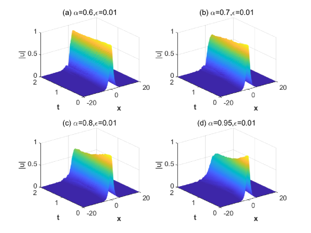
Figure 1: The evolution of the solution $u(x,t)$ with the initial condition $u(x,0)=\mathrm{sech}(x)\mathrm{exp}(2ix)$, where $\epsilon=0.01$, $\sigma=1,\lambda=1$ and different $\alpha=0.6,0.7,0.8,0.95$.

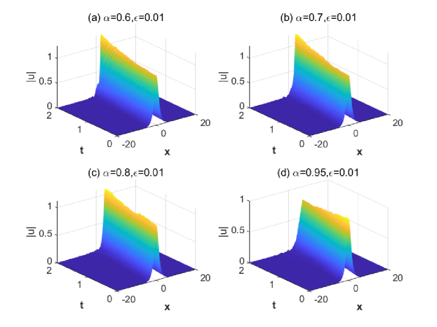
Figure 2: The evolution of the solution $u(x,t)$ with the initial condition $u(x,0)=\mathrm{sech}(x)\mathrm{exp}(2ix)$, where $\epsilon=0.01$, $\sigma=1$, $\lambda=-1$ and different $\alpha=0.6,0.7,0.8,0.95$.

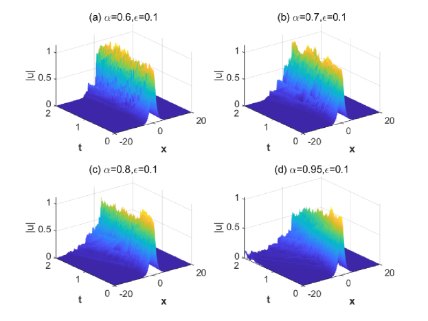
Figure 3: The evolution of the solution $u(x,t)$ with the initial condition $u(x,0)=\mathrm{sech}(x)\mathrm{exp}(2ix)$, where $\epsilon=0.1$, $\sigma=1$, $\lambda=1$ and different $\alpha=0.6,0.7,0.8,0.95$.

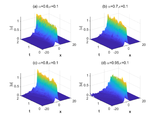
Figure 4: The evolution of the solution $u(x,t)$ with the initial condition $u(x,0)=\mathrm{sech}(x)\mathrm{exp}(2ix)$, where $\epsilon=0.1$, $\sigma=1$, $\lambda=-1$ and different $\alpha=0.6,0.7,0.8,0.95$.

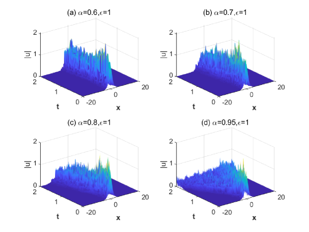
Figure 5: The evolution of the solution $u(x,t)$ with the initial condition $u(x,0)=\mathrm{sech}(x)\mathrm{exp}(2ix)$, where $\epsilon=1$, $\sigma=1$, $\lambda=1$ and different $\alpha=0.6,0.7,0.8,0.95$.

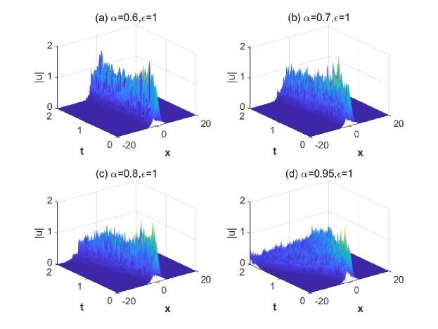
Figure 6: The evolution of the solution $u(x,t)$ with the initial condition $u(x,0)=\mathrm{sech}(x)\mathrm{exp}(2ix)$, where $\epsilon=1$, $\sigma=1$, $\lambda=-1$ and different $\alpha=0.6,0.7,0.8,0.95$.

In Table 1, the global mass conservation is presented with different powers $\alpha=0.6,0.75,0.9$, $\epsilon=0.01$, $\sigma=1$, and various time values, denoted as $t$. The table illustrates that our numerical method maintains mass conservation.

Time	$\alpha=0.6$	$\alpha=0.75$	$\alpha=0.9$
$t=0$	1.414211518677561	1.414211518677561	1.414211518677561
$t=2$	1.414211518677503	1.414211518677491	1.414211518677486
$t=4$	1.414211518677513	1.414211518677470	1.414211518677408
$t=6$	1.414211518677494	1.414211518677484	1.414211518677351
$t=8$	1.414211518677447	1.414211518677443	1.414211518677257
$t=10$	1.414211518677408	1.414211518677402	1.414211518677153

Table 1: The value of mass $M(t)$ at different time $t$ for the equation (4.28) based on a single sample path .

Figure 7 shows the energy evolution with $\alpha=0.6$, $\lambda=-1$ and $\varepsilon=0.01$, by using the midpoint scheme and the same initial condition. We can find that the energy is no longer constant in the stochastic case.

Figure 7: The energy of 10 sample orbits and the averaged energy of 500 sample orbits.

5 A mass-preserving splitting scheme

Because the midpoint scheme (4.22) is implicit, we expect to provide an explicit numerical scheme to solve the one-dimensional stochastic fractional nonlinear Schrödinger equation (1.1) with $\sigma=0$, and give the error analysis. We consider the following nonlinear equation

$$idu =\lambda udt+u\circ dW(t).$$ (5.1)

The following result comes from [21, Theorem 2.1].

Lemma 12.

Assume that $\Phi\in L_{HS}(L^{2},H^{2\alpha})$ and $u(x,0)$ is $\mathcal{F}_{0}$-measurable $L^{2}$-valued random variables. The following $u(x,t)$ is a solution of (5.1):

$$u(x,t)=u(x,0)\exp\{-it\lambda-iW(x,t)\}.$$ (5.2)

In the following, we can define the following splitting scheme initialized with $u_{0}=u(x,0),t_{n}=n\delta t$,

$$u_{n}=\exp\{-i\delta t(-\Delta)^{\alpha}\}\cdot\exp\left\{-i\delta t\lambda-i\left[W(x,t_{n})-W(x,t_{n-1})\right]\right\}u_{n-1}.$$ (5.3)

It is obvious that $\|u_{n}\|^{2}_{L^{2}}=\|u_{n-1}\|^{2}_{L^{2}}$. Therefore we have the following lemma.

Lemma 13.

Assume that $\Phi\in L_{HS}(L^{2},H^{2\alpha})$. For any $\delta t$ and $n$, the scheme (5.3) satisfies

$$\|u_{n}\|^{2}_{L^{2}}=\|u_{n-1}\|^{2}_{L^{2}}.$$ (5.4)

Let us state the following result.

Lemma 14.

For any $\kappa\geqslant 0$,

$$\left\|e^{-\mathrm{i}t(-\Delta)^{\alpha}}w_{0}\right\|_{H^{\kappa}} =\left\|w_{0}\right\|_{H^{\kappa}},\quad\left\|(-\Delta)^{\alpha}\left(e^{-\mathrm{i}t(-\Delta)^{\alpha}}w_{0}\right)\right\|_{H^{\kappa}}=\left\|(-\Delta)^{\alpha}w_{0}\right\|_{H^{\kappa}},$$ (5.5)

$$\left\|\left(e^{-\mathrm{i}t(-\Delta)^{\alpha}}-I\right)w_{0}\right\|_{H^{\kappa}} \leqslant t\left\|(-\Delta)^{\alpha}w_{0}\right\|_{H^{\kappa}}.$$

Proof. Let $\hat{w}_{0}(\xi)=\frac{1}{2\pi}\int_{\mathbb{R}}w_{0}(x)e^{-\mathrm{i}x\cdot\xi}\mathrm{d}x$ be the Fourier transform of $w_{0}$. The Fourier transform of $e^{-\mathrm{i}t(-\Delta)^{\alpha}}w_{0}$ is $e^{-\mathrm{i}t|\xi|^{2\alpha}}\hat{w}_{0}$. The Fourier transform of $(-\Delta)^{\alpha}\left(e^{-\mathrm{i}t(-\Delta)^{\alpha}}w_{0}\right)$ is $e^{-\mathrm{i}t|\xi|^{2\alpha}}|\xi|^{2\alpha}\hat{w}_{0}$. So, the second result follows from the equivalent definition of $H^{\sigma}$. To prove the third result, note that

$$\frac{\left\|\left(e^{-\mathrm{i}t(-\Delta)^{\alpha}}-I\right)w_{0}\right\|_{H^{\kappa}}^{2}}{\left\|(-\Delta)^{\alpha}w_{0}\right\|_{H^{\kappa}}^{2}}=\frac{\left\|\left(1+|\xi|^{2\sigma}\right)^{1/2}\left(e^{\mathrm{i}t|\xi|^{2\alpha}}-1\right)\hat{w}_{0}\right\|_{L^{2}}^{2}}{\left\|\left(1+|\xi|^{2\sigma}\right)^{1/2}|\xi|^{2\alpha}\hat{w}_{0}\right\|_{L^{2}}^{2}}.$$

Hence, it follows from

$$\left|e^{\mathrm{i}t|\xi|^{2\alpha}}-1\right|=\left|\int_{0}^{t}(\mathrm{~{}d}/\mathrm{d}s)e^{\mathrm{i}s|\xi|^{2\alpha}}\mathrm{~{}d}s\right|=\left|\int_{0}^{t}\mathrm{i}\left|\xi\right|^{2\alpha}e^{\mathrm{i}s|\xi|^{2\alpha}}\mathrm{~{}d}s\right|\leqslant t|\xi|^{2\alpha}.$$

In the following, we introduce an auxiliary continuous function $v_{N}(x,t)$ with $t\in[0,T)$ and on any interval $[t_{n-1},t_{n})$,

$$v_{N}(x,t)=\left\{\begin{aligned} &e^{\left[-i\lambda(t-t_{n-1})\right]-i\left[W(t)-W(t_{n-1})\right]}v_{N}(x,t_{n-1}),~{}~{}t\in[t_{n-1},t_{n}),\\ &e^{-i\delta t(-\Delta)^{\alpha}}\lim_{t\uparrow t_{n}}v_{N}(x,t),~{}~{}~{}~{}t=t_{n}.\end{aligned}\right.$$ (5.6)

where $v_{N}(x,0)=u(x,0),~{}\delta t=\frac{T}{N}$.

Therefore for any $t\in[t_{n-1},t_{n})$, we have

$$dv_{N}(x,t)=-i\lambda v_{N}(x,t)dt-iv_{N}(x,t)\circ dW(t).$$

Rewriting the above equation into integral form, we get

$$v_{N}(x,t)=v_{N}(x,t_{n-1})-i\lambda\int^{t}_{t_{n-1}}v_{N}(x,s)ds-i\int^{t}_{t_{n-1}}v_{N}(x,s)\circ dW(s).$$ (5.7)

Combing (5.6) and (5.7), we obtain

$$v_{N}(x,t_{n})=e^{-i\delta t(-\Delta)^{\alpha}}\left[v_{N}(x,t_{n-1})-i\lambda\int^{t_{n}}_{t_{n-1}}v_{N}(x,s)ds-i\int^{t_{n}}_{t_{n-1}}v_{N}(x,s)\circ dW(s)\right].$$ (5.8)

Using the above recursive formula (5.8) and equality (5.7), for any $t\in[t_{n-1},t_{n})$, we have

$$v_{N}(x,t)=e^{-it_{n-1}(-\Delta)^{\alpha}}u_{0}-i\lambda\int^{t}_{0}S_{N,n,t}(s)v_{N}(x,s)ds-i\int^{t}_{0}S_{N,n,t}(s)v_{N}(x,s)\circ dW(s),$$ (5.9)

where

$$S_{N,n,t}(s)=\sum_{l=1}^{n-1}I_{[t_{n-1-l},t_{n-l})}(s)e^{-i\left(l\delta t\right)(-\Delta)^{\alpha}}+I_{[t_{n-1},t)}(s).$$

By equation (5.9) and the definition of $v_{N}(x,t)$ with $t=t_{n}$, when $t$ approaches $t_{n}$, we have

$$v_{N}(x,t_{n}) =e^{-it_{n}(-\Delta)^{\alpha}}u_{0}-i\lambda\int^{t_{n}}_{0}S(t_{n}-s)v_{N}(x,s)ds-i\int^{t_{n}}_{0}S(t_{n}-s)v_{N}(x,s)\circ dW(s)$$

$$+i\lambda\int^{t_{n}}_{0}\left[S(t_{n}-s)-S_{N,n+1,t_{n}}(s)\right]v_{N}(x,s)ds+i\int^{t_{n}}_{0}\left[S(t_{n}-s)-S_{N,n+1,t_{n}}(s)\right]v_{N}(x,s)\circ dW(s).$$

The exact solution of (1.1) can be written as

$$u(x,t)=S(t)u_{0}-i\lambda\int_{0}^{t}S(t-s)u(s)ds-i\int_{0}^{t}S(t-s)(u(x,s)\circ dW(s)),$$ (5.10)

where $S(t)=e^{-it(-\Delta)^{\alpha}}$.

The following lemma comes from [12, Lemma 2.1].

Lemma 15.

Let $H$ be a separable Hilbert space and $E,F$ two separable Banach spaces. Given $K\in L_{HS}(H,E)$ and $J\in L(E;F)$, then $JK\in L_{HS}(H,F)$ and

$$\|JK\|_{L_{HS}(H,F)}\leq\|J\|_{L(E,F)}\|K\|_{L_{HS}(H,E)}.$$ (5.11)

Next, we give the Leibniz and chain rule for fractional derivatives, see [39, 40, 41] and the references therein.

Lemma 16.

Let $\alpha\in(0,1)$, $1<p\leq\infty$, and $1<p_{1},p_{2},p_{3},p_{4}\leq\infty$ with $\frac{1}{p}=\frac{1}{p_{1}}+\frac{1}{p_{2}}$, $\frac{1}{p}=\frac{1}{p_{3}}+\frac{1}{p_{4}}$, and let $f,g\in\mathcal{S}(\mathbb{R})$, then

$$\left\|(-\Delta)^{\alpha}(fg)\right|_{L^{p}(\mathbb{R})}\leq C\|(-\Delta)^{\alpha}f\|_{L^{p_{1}}(\mathbb{R})}\|g\|_{L^{p_{2}}(\mathbb{R})}+C\|(-\Delta)^{\alpha}g\|_{L^{p_{3}}(\mathbb{R})}\|g\|_{L^{p_{4}}(\mathbb{R})};$$ (5.12)

In the following, we aim to give the convergence order of the proposed scheme.

Let $r(t,x)=u(t,x)-v_{N}(x,t)$, if $t\in[t_{n-1},t_{n})$, then we have

$$r(t,x) =\left(e^{-i(t-t_{n-1})(-\Delta)^{\alpha}}-I\right)e^{-it_{n-1}(-\Delta)^{\alpha}}u_{0}$$ (5.13)

$$-i\int^{t}_{0}S_{N,n,t}(s)r(s,x)\circ dW(s)-i\int^{t}_{0}\left[S(t-s)-S_{N,n,t}(s)\right]u(s,x)\circ dW(s)$$

$$-i\lambda\int^{t}_{0}S_{N,n,t}(s)r(s,x)ds-i\lambda\int^{t}_{0}\left[S(t-s)-S_{N,n,t}(s)\right]u(s,x)ds$$

$$=I_{1}+I_{2}+I_{3}+I_{4}+I_{5}.$$

For the term $I_{1}$, by Lemma 14, we have

$$\left\|I_{1}\right\|^{2}_{L^{2}} \leq\delta t^{2}\left\|(-\Delta)^{\alpha}\left(e^{-it_{n-1}(-\Delta)^{\alpha}}u_{0}\right)\right\|^{2}_{L^{2}} \leq\delta t^{2}\left\|u_{0}\right\|^{2}_{H^{2\alpha}}.$$

For the term $I_{2}$, note that

$$i\int^{t}_{0}S_{N,n,t}(s)r(s,x)\circ dW(s) =i\int^{t}_{0}S_{N,n,t}(s)r(s,x)dW(s)+\frac{1}{2}\int^{t}_{0}S_{N,n,t}(s)r(s,x)F_{\Phi}ds$$

$$:=I_{21}+I_{22}.$$

By Lemma 14 and embedding theorem [54, Remark 1.4.1(v)]( i.e. $H^{2\alpha}\hookrightarrow L^{\infty}$), we have

$$\|J\|_{L(H^{2\alpha},L^{2})} =\sup_{\omega}\frac{\|e^{-i\left(l\delta t\right)(-\Delta)^{\alpha}}(r(s)\omega)\|_{L^{2}}}{\|\omega\|_{H^{2\alpha}}}=\sup_{\omega}\frac{\|r(s)\omega\|_{L^{2}}}{\|\omega\|_{H^{2\alpha}}}$$ (5.14)

$$\leq\sup_{\omega}\frac{\|r(s)\|_{L^{2}}\cdot\|\omega\|_{L^{\infty}}}{\|\omega\|_{H^{2\alpha}}}$$

$$\leq C\|r(s)\|_{L^{2}},$$

where the operator $J$ is defined by $J\omega=e^{-i\left(l\delta t\right)(-\Delta)^{\alpha}}(r(s)\omega)$. By Lemma 15 and inequality (5.14), we have

$$\|e^{-i\left(l\delta t\right)(-\Delta)^{\alpha}}(r(s)\Phi)\|_{L_{HS}(L^{2},L^{2})}\leq\|\Phi\|_{{L_{HS}}(L^{2},H^{2\alpha})}\|J\|_{L(H^{2\alpha},L^{2})}\leq C\|\Phi\|_{{L_{HS}}(L^{2},H^{2\alpha})}\cdot\|r(s)\|_{L^{2}}.$$ (5.15)

In the following, we give the estimates of $I_{21}$ and $I_{22}$, respectively. To estimate $I_{21}$, we can use the Burkholder inequality [55, Lemma 9.2], inequalities (5.14) and (5.15) to obtain

$$\mathbb{E}\sup_{0\leq s\leq t}\|I_{21}(s)\|^{2}_{L^{2}} \leq 4\mathbb{E}\int^{t}_{0}\|S_{N,n,t}(s)r(s,x)\Phi\|^{2}_{L_{L_{HS}(L^{2},L^{2})}}ds$$

$$=4\mathbb{E}\sum^{n-1}_{j=1}\int^{t_{n-j}}_{t_{n-j-1}}\|S_{N,n,t}(s)r(s,x)\Phi\|^{2}_{L_{HS}(L^{2},L^{2})}ds+4\mathbb{E}\int^{t}_{t_{n-1}}\|S_{N,n,t}(s)r(s,x)\Phi\|^{2}_{L_{HS}(L^{2},L^{2})}ds$$

$$\leq 4C\|\Phi\|_{{L_{HS}}(L^{2},H^{2\alpha})}\int^{t}_{0}\mathbb{E}\|r(s)\|^{2}_{L^{2}}ds.$$

Similarly,

$$\|I_{22}\|^{2}_{L^{2}} \leq\frac{T}{4}\|F_{\Phi}\|^{2}_{L^{\infty}}\int^{t}_{0}\|r(s,x)\|^{2}_{L^{2}}ds$$

$$\leq\frac{T}{4}\|{\Phi}\|_{L_{HS}(L^{2},H^{2\alpha})}^{4}\int^{t}_{0}\|r(s,x)\|^{2}_{L^{2}}ds.$$

Therefore we have

$$\mathbb{E}\sup_{0\leq s\leq t}\|I_{2}\|^{2}_{L^{2}}\leq 4C\|\Phi\|_{{L_{HS}}(L^{2},H^{2\alpha})}\int^{t}_{0}\mathbb{E}\|r(s)\|^{2}_{L^{2}}ds+\frac{T}{4}\|{\Phi}\|_{L_{HS}(L^{2},H^{2\alpha})}^{2}\int^{t}_{0}\|r(s,x)\|^{2}_{L^{2}}ds.$$

For the term $I_{3}$, utilizing the equivalence relationship between Itô stochastic integral and Stratonovich integral, we have

$$i\int^{t}_{0}\left[S(t-s)-S_{N,n,t}(s)\right]u(s,x)\circ dW(s) =i\int^{t}_{0}\left[S(t-s)-S_{N,n,t}(s)\right]u(s,x)dW(s)+\frac{1}{2}\int^{t}_{0}\left[S(t-s)-S_{N,n,t}(s)\right]u(s,x)F_{\Phi}ds$$

$$:=I_{31}+I_{32}.$$

Note that when $t\in[t_{n-1},t_{n})$ and $s\in[t_{n-1-j},t_{n-j})$, then $|t-s-j\delta t|\leq 2\delta t$. Then by Lemma 14, Leibniz rule for fractional derivative (5.12) and $H^{2\alpha}\hookrightarrow L^{\infty}$, we have

$$\|\left[S(t-s)-S_{N,n,t}(s)\right]u(s)\|_{L({H^{2\alpha},L^{2}})} =\sup_{\omega}\frac{\|\left(e^{-i\left(t-s-j\delta t\right)(-\Delta)^{\alpha}}-I\right)e^{-i\left(j\delta t\right)(-\Delta)^{\alpha}}(u(s)\omega)\|_{L^{2}}}{\|\omega\|_{H^{2\alpha}}}$$

$$\leq 2\delta t\sup_{\omega}\frac{\|(-\Delta)^{\alpha}(u(s)\omega)\|_{L^{2}}}{\|\omega\|_{H^{2\alpha}}}$$

$$\leq C\delta t\sup_{\omega}\frac{\|(-\Delta)^{\alpha}u(s)\|_{L^{2}}\cdot\|\omega\|_{L^{\infty}}+\|(-\Delta)^{\alpha}\omega\|_{L^{2}}\cdot\|u(s)\|_{L^{\infty}}}{\|\omega\|_{H^{2\alpha}}}$$

$$\leq C\delta t\sup_{\omega}\frac{\|u(s)\|_{H^{2\alpha}}\cdot\|\omega\|_{H^{2\alpha}}+\|\omega\|_{H^{2\alpha}}\cdot\|u(s)\|_{H^{2\alpha}}}{\|\omega\|_{H^{2\alpha}}}$$

$$\leq C\delta t\|u(s)\|_{H^{2\alpha}}.$$

To estimate $I_{31}$, by the similar argument [12, Lemma 3.2], Lemma 14 and Lemma 15, we have

$$\mathbb{E}\sup_{0\leq s\leq t}\|I_{31}(s)\|^{2}_{L^{2}} \leq 4\mathbb{E}\int^{t}_{0}\|\left[S(t-s)-S_{N,n,t}(s)\right]u(s,x)\Phi\|_{L_{HS}(L^{2},L^{2})}^{2}ds$$

$$\leq 4\|\Phi\|^{2}_{{L}_{HS}(L^{2},H^{2\alpha})}\mathbb{E}\int^{t}_{0}\|\left[S(t-s)-S_{N,n,t}(s)\right]u(s,x)\|^{2}_{L(H^{2\alpha},L^{2})}ds$$

$$\leq C\|\Phi\|^{2}_{{L}_{HS}(L^{2},H^{2\alpha})}\delta t^{2}\mathbb{E}\int^{t}_{0}\|u(s,x)\|^{2}_{H^{2\alpha}}ds.$$

Similarly, we have

$$\mathbb{E}\sup_{0\leq s\leq t}\|I_{32}(s)\|^{2}_{L^{2}} \leq CT\mathbb{E}\int^{t}_{0}\|\left[S(t-s)-S_{N,n,t}(s)\right]u(s,x)F_{\Phi}\|^{2}ds$$

$$\leq CT\|F_{\Phi}\|^{2}_{L^{\infty}}\mathbb{E}\int^{t}_{0}\delta t^{2}\left\|(-\Delta)^{\alpha}\left(u(s,x)\right)\right\|^{2}_{L^{2}}ds$$

$$\leq CT\|{\Phi}\|_{L_{HS}(L^{2},H^{2\alpha})}^{4}\delta t^{2}\mathbb{E}\int^{t}_{0}\|u(s,x)\|^{2}_{H^{2\alpha}}ds.$$

Therefore we have

$$\mathbb{E}\sup_{0\leq s\leq t}\|I_{3}\|^{2}_{L^{2}} \leq C\left(\|\Phi\|^{2}_{L(L^{2},H^{2\alpha})}+T\|{\Phi}\|_{L_{HS}(L^{2},H^{2\alpha})}^{4}\right)\delta t^{2}\mathbb{E}\int^{t}_{0}\|u(s,x)\|^{2}_{H^{2\alpha}}ds.$$

For the term $I_{4}$, by Lemma 14, we have

$$\mathbb{E}\sup_{0\leq s\leq t}\|I_{4}\|^{2}_{L^{2}} \leq CT\mathbb{E}\int^{t}_{0}\left\|S_{N,n,t}(s)r(s,x)\right\|^{2}_{L^{2}}ds$$

$$\leq CT\int^{t}_{0}\mathbb{E}\|r(s,x)\|^{2}_{L^{2}}ds.$$

For the term $I_{5}$, by the definition of $S_{N,n,t}$, we have

$$\|I_{5}(t)\|^{2}_{L^{2}} \leq CT\int^{t}_{0}\left\|\left[S(t-s)-S_{N,n,t}(s)\right]u(s,x)\right\|^{2}_{L^{2}}ds.$$

When $t\in[t_{n-1},t_{n})$ and $s\in[t_{n-1-j},t_{n-j})$, then $|t-s-j\delta t|\leq\delta t$. By Lemma 14, we further have

$$\int^{t}_{0}\left\|\left[S(t-s)-S_{N,n,t}(s)\right]u(s,x)\right\|^{2}_{L^{2}}ds \leq\delta t^{2}\int^{t}_{0}\left\|(-\Delta)^{\alpha}\left(e^{-i\left(j\delta t\right)(-\Delta)^{\alpha}}u(s,x)\right)\right\|^{2}_{L^{2}}ds$$

$$=\delta t^{2}\int^{t}_{0}\left\|(-\Delta)^{\alpha}u(s,x)\right\|^{2}_{L^{2}}ds$$

$$=\delta t^{2}\int^{t}_{0}\left\|u(s,x)\right\|^{2}_{H^{2\alpha}}ds$$

By Theorem 2, we have

$$\mathbb{E}\sup_{0\leq s\leq t}\|I_{5}(t)\|^{2}_{L^{2}}\leq CT\delta t^{2}.$$

Let $r=u-v_{N}$ with $v_{N}$ satisfying $v_{N}\left(t_{n}\right)=u_{n}$. From (5.13), we get

$$\mathbb{E}\sup_{0\leqslant t\leqslant\tau}\|r(t)\|_{L^{2}}^{2}\leqslant\sum_{j=1}^{5}\mathbb{E}\sup_{0\leqslant t\leqslant\tau}\left\|I_{j}(t)\right\|_{L^{2}}^{2}.$$

Recall these estimates for the term $I_{1}$-$I_{5}$, we know that there are constants $C_{2}$ and $C_{3}$ such that for $t\in[t_{n-1},t_{n})$,

$$\mathbb{E}\sup_{0\leqslant t\leqslant\tau}\|r(t)\|_{L^{2}}^{2}\leqslant C_{2}\int_{0}^{\tau}\left(\mathbb{E}\sup_{0\leqslant s\leqslant t}\|r(s)\|_{L^{2}}^{2}\right)\mathrm{d}t+C_{3}\delta t^{2}.$$

So using Gronwall’s inequality, we obtain the following theorem.

Theorem 5.

(Convergence rate of the splitting scheme). Consider the scheme (2.9)-(2.10) for the equation (1.1). Assume that $\Phi\in L_{HS}\left(L^{2}\left(\mathbb{R}\right),H^{2\alpha}\left(\mathbb{R}\right)\right)$, $\sigma=0$, and $u_{0}$ is an $\mathcal{F}_{0}$-measurable random variable with $\mathbb{E}\left\|u_{0}\right\|_{H^{2\alpha}}^{2}<\infty$. Then, for any $T$, there exists a constant $C$ such that, for any $\delta t$,

$$\mathbb{E}\max_{n=0,1,\ldots,[T/\delta t]}\left\|u\left(t_{n}\right)-u_{n}\right\|_{L^{2}}\leqslant C\delta t.$$ (5.16)

5.1 Numerical example

In this section, we consider the following stochastic fractional nonlinear Schrödinger equations to illustrate the efficiency of the splitting scheme and show the convergence order for the splitting scheme with spatially regular noise.

$$\left\{\begin{aligned} &idu-\left[(-\Delta)^{\alpha}u+\lambda u\right]dt=\varepsilon u\circ dW(t),\quad t\geq 0,\\ &u(0)=\mathrm{sech}(x)\mathrm{exp}(2ix),\end{aligned}\right.$$ (5.17)

The real-valued Wiener process $W(t)=\sum_{l=1}^{100}\frac{1}{l}\sin(\pi lx)\beta_{l}(t)$, where $\{\beta_{l}(t)\}^{100}_{l=1}$ are a family of independent $\mathbb{R}$-valued Wiener processes. Table 2 provides the error and convergence rates for the stochastic nonlinear Schrödinger equation with $\alpha=0.75$, $\Delta x=0.1$, $\epsilon=0.01$, $\sigma=0$, $T=0.4$, $\lambda=-1$, and the domain $[0,40]$. This table shows the error as:

$$Error=\frac{1}{M}\sum\limits_{i=1}^{M}\max\limits_{n=0,1,\ldots,[T/\delta t]}||u_{ref}^{i}(n\Delta t)-u_{r}^{i}(n\Delta t)||_{l^{2}},$$

where $u_{r}^{i}(n\Delta t)$ is the numerical solution for different time steps $\Delta t=\frac{0.01}{2^{r}}$, $r=0,1,...,4$, and $u_{ref}^{i}(n\Delta t)$ is the reference solution for $\Delta t=\frac{0.01}{2^{5}}$ as the exact solution is unknown. Here, $M=500$ represents the number of sample trajectories. It can be observed that the convergence order is approximately 1, which aligns with our theoretical results.

$\Delta t$	0.01	$\frac{0.01}{2}$	$\frac{0.01}{2^{2}}$	$\frac{0.01}{2^{3}}$	$\frac{0.01}{2^{4}}$
Error	2.681e-2	1.345e-2	6.448e-3	2.861e-3	1.087e-3
order	0.995	1.061	1.172	1.396

Table 2: The error and convergence between numerical solution and reference solution for different $\Delta t$.

6 Acknowledgments

The authors would like to thank Yichun Zhu (Chinese Academy of Sciences) for helpful discussions. The research of X. Wang is supported by the Natural Science Foundation of Henan Province of China (Grant No. 232300420110).

References

• [1] S. Longhi, Fractional Schrödinger equation in optics, Opt. Lett., 40: 1117-1120, 2015.
• [2] S. Liu, Y. Zhang, B. A. Malomed, E. Karimi, Experimental realizations of the fractional Schrödinger equation in the temporal domain, Nat. Commun., 14: 222, 2023.
• [3] A. D. Ionescu, F. Pusateri, Nonlinear fractional Schrödinger equations in one dimension, J. Funct. Anal., 266: 139-176, 2014.
• [4] N. Laskin, Fractional Schrödinger equation, Phys. Rev. E, 66: 056108, 2002.
• [5] K. Kirkpatrick, E. Lenzmann, Gigliola Staffilani, On the continuum limit for discrete NLS with long-range lattice interactions, Phys. Rev. E, 66: 056108, 2002.
• [6] A. Ionescu, F. Pusateri, Nonlinear fractional Schrödinger equations in one dimension, J. Funct. Anal., 266: 139-176, 2014.
• [7] X. Shang, J. Zhang, Ground states for fractional Schrödinger equation with critical growth, Nonlinearity, 27: 187-207, 2014.
• [8] B. Choi, A. Ceves, Continuum limit of $2D$ fractional nonlinear Schrödinger equation, J. Evol. Equ., 23: 30, 2023.
• [9] R. L. Frank, E. Lenzmann, L. Silvestre, Uniqueness of radial solutions for the fractional Laplacian, Commun. Pur. Appl. Math., 69, 1671-1726, 2016.
• [10] P. Wang, C. Huang, An energy conservative difference scheme for the nonlinear fractional Schrödinger equations, J. Comput. Phy., 293, 238-251, 2015.
• [11] S. Duo, Y. Zhang, Mass-conservative Fourier spectral methods for solving the fractional nonlinear Schrödinger equation, Comput. Math. with Appl., 71, 2257-2271, 2016.
• [12] A. de Bouard, A. Debussche, A stochastic nonlinear Schrödinger equation with multiplicative noise, Commun. Math. Phys., 205: 121-127, 1999.
• [13] A. de Bouard, A. Debussche, Blow-up for the stochastic nonlinear Schrödinger equation with multiplicative noise, Ann. Probab., 33: 1078-1110, 2005.
• [14] S. Herr, M. Röckner, D. Zhang, Scatter for stochastic nonlinear Schrödinger equations, Commun. Math. Phys., 368: 843-884, 2019.
• [15] V. Barbu, M. Röckner, D. Zhang, Stochastic nonlinear Schrödinger equations: No blow-up in the non-conservative case, J. Differ. Equ., 263: 7919-7940, 2017.
• [16] Y. Deng, A. R. Nahmod, H. Yue, Random tensors, propagation of randomness, and nonlinear dispersive equations, Invent. Math., 228: 539-686, 2022.
• [17] A. Debussche, L. D. Menza, Numerical simulation of focusing stochastic nonlinear Schrödinger equations, Physica D, 162: 131-154, 2002.
• [18] A. de Bouard, A. Debussche, A semi-discrete scheme for the stochastic nonlinear Schrödinger equation, Numer. Math., 96: 733-770, 2004.
• [19] J. Cui, J. Hong, Z. Liu, W. Zhou, Strong convergence rate of splitting schemes for stochastic nonlinear Schrödinger equations, J. Differ. Equ., 266: 5625-5663, 2019.
• [20] J. Liu, Order of convergence of splitting schemes for both deterministic and stochastic nonlinear Schrödinger equations, SIAM J. Numer. Anal., 51: 1911-1932, 2013.
• [21] J. Liu, A mass-preserving splitting scheme for the stochastic Schrödinger equation with multiplicative noise, IMA J. Numer. Anal., 33: 1469-1479, 2013.
• [22] C. Chen, J. Hong, Symplectic Runge-Kutta semi-discretization for stochastic schrödinger equation, SIAM J. Numer. Anal., 54: 2569-2593, 2016.
• [23] Rikard Anton, David Cohen, Exponential integrators for stochastic Schrödinger equations driven by Itô noise, J. Comput. Math., 36: 276-309, 2018.
• [24] J. Cui, J. Hong, Z. Liu, W. Zhou, Stochastic symplectic and multi-symplectic methods for nonlinear schrödinger equation with white noise dispersion, J. Comput. Phy., 342, 267-285, 2017.
• [25] J. Cui, J. Hong, Analysis of a splitting scheme for damped stochastic nonlinear Schrödinger equation with multiplicative noise, SIAM J. Numer. Anal., 56: 2045-2069, 2018.
• [26] J. Cui, J. Hong, Z. Liu, Strong convergence rate of finite difference approximations for stochastic cubic Schrödinger equations, J. Differ. Equ., 263: 3687-3713, 2017.
• [27] C.-Edouard Bréhier, D. Cohen, Analysis of a splitting scheme for a class of nonlinear stochastic Schrödinger equations, Appl. Numer. Math., 186: 57-83, 2023.
• [28] H. Yuan, G. Chen, Martingale solutions of stochastic fractional nonlinear Schrödinger equation on a bounded interval, J. Differ. Equ., 263: 7919-7940, 2017.
• [29] A. Zhang, Y. Zhang, X. Wang, Z. Wang, J. Duan, The stochastic fractional Strichartz estimate and blow-up for Schrödinger equation, https://arxiv.org/abs/2308.10270.
• [30] Z. Brzeźniak, W. Liu, J. Zhu, The stochastic Strichartz estimates and stochastic nonlinear Schrödinger equations driven by Lévy noise, J. Funct. Anal., 281: 109021, 2021.
• [31] J. Wang, J. Zhai, J. Zhu, The stochastic nonlinear Schrödinger equations driven by pure jump noise. Stat. Probab. Lett., 197, 109810, 2023.
• [32] G. Milstein, Yu. Repin, M. Tretyakov, Symplectic integration of Hamiltonian systems with additive noise, SIAM J. Numer. Anal., 40: 1583-1604, 2002.
• [33] P. Wei, Y. Chao, J. Duan, Hamiltonian systems with Lévy noise: Symplecticity, Hamilton’s principle and averaging principle, Physica D, 292: 69-83, 2019.
• [34] J. Duan, An Introduction to Stochastic Dynamics, Cambridge University Press, 2015.
• [35] E. Di Nezza, G. Palatucci, E. Valdinoci, Hitchhiker’s guide to the fractional Sobolev spaces, Bull. Sci. Math., 136: 521-573, 2012.
• [36] V. D. Dinh, A study on blowup solutions to the focusing $L^{2}$-supercritical nonlinear fractional Schrödinger equation, J. Math. Phys., 59: 071506, 2018.
• [37] M. Christ, I. Weinstein, Dispersion of small amplitude solutions of the generalized Korteweg-de Vries equation, J. Funct. Anal. 100: 87-109, 1991.
• [38] N. N. Vakhania, V. I. Taireladze, S. A. Chobanyan, Probability and distribution on Banach space, Springer Science $\&$ Business Media, 1987.
• [39] C. Kenig, G. Ponce, L. Vega, Well-posedness and scattering results for the generalized Korteweg-de Vries equation via contraction principle, Commun. Pure Appl. Math., 46: 527-620, 1993.
• [40] J. Bourgain, D. Li, On an endpoint Kato-Ponce inequality, Differ. Integral Equ., 27: 1037-1072, 2014.
• [41] D. Li, On Kato-Ponce and fractional Leibniz, Rev. Mat. Iberoam, 35: 23-100, 2019.
• [42] A. de Bouard, A. Debussche, The stochastic non-linear Schrödinger equation in $H^{1}$, Stoch. Anal. Appl., 21: 197-126, 2003.
• [43] V. Barbu, M. Roeckner, D. Zhang, Stochastic nonlinear Schroedinger equations, Nonlinear Anal., 136: 168-194, 2016.
• [44] V. Dinh, On blow-up solutions to the focusing mass-critical nonlinear fractional Schrödinger equation, Commun. Pur. Appl. Anal., 18: 689-708, 2019.
• [45] P. Wang, C. Huang Structure-preserving numerical method for the fractional Schrödinger equation, Appl. Numer. Math., 129: 137-158, 2018.
• [46] J. Shen, T. Tang, L. L. Wang, Spectral Methods: Algorithm, Analysis and Applications, Springer Series in Computational Mathematics 41, Springer, Berlin Heidelberg, 2011.
• [47] D. Cohen, Conservation properties of numerical integrators for highly oscillatory Hamiltonian systems. IMA J. Numer. Anal., 26: 34-59, 2006.
• [48] D. Cohen, Conservation of energy, momentum and actions in numerical discretizations of non-linear wave equation. Numer. Math., 110: 113-143, 2008.
• [49] G. N. Milstein, Yu. M. Repin and M. V. Tretyakov, Symplectic integration of Hamiltonian systems with additive noise. SIAM J. Numer. Anal., 39: 2066-2088, 2002.
• [50] C. A. Anton, Y. S. Wong and J. Deng, Symplectic schemes for stochastic Hamiltonian systems preserving Hamiltonian functions. Int. J. Numer. Anal. Model., 11: 427-451, 2014.
• [51] K. Burrage and P. M. Burrage, Low rank Runge-Kutta methods, symplecticity and stochastic Hamiltonian problems with additive noise. J. Comput. Appl. Math., 236: 3920-3930, 2012.
• [52] J. Hong, L. Miao and L. Zhang Convergence analysis of a symplectic semi-discretization for stochastic NLS equation with quadratic potential. Discrete Contin. Dyn. Syst.Ser. B, 24: 4295-4315, 2019.
• [53] G. Milstein and M. Tretyakov, Stochastic Numerics for Mathematical Physics, Kluwer Academic Publishers, 1995.
• [54] T. Cazenave, Semilinear Schrodinger Equations, American Mathematical Society, Courant Institute of Mathematical Sciences, 2003.
• [55] D. Prato and J. Zabczyk Stochastic Equations in Infinite Dimensions. Cambridge: Cambridge University Press, 1992.