The McCormick martingale optimal transport

Abstract

Martingale optimal transport (MOT) often yields broad price bounds for options, constraining their practical applicability. In this study, we extend MOT by incorporating causality constraints among assets, inspired by the nonanticipativity condition of stochastic processes. However, this introduces a computationally challenging bilinear program. To tackle this issue, we propose McCormick relaxations to ease the bicausal formulation and refer to it as McCormick MOT. The primal attainment and strong duality of McCormick MOT are established under standard assumptions. Empirically, McCormick MOT demonstrates the capability to narrow price bounds, achieving an average reduction of 1% or 4%. The degree of improvement depends on the payoffs of the options and the liquidity of the relevant vanilla options.
Keywords: Martingale optimal transport, causal optimal transport, bilinear constraints, McCormick relaxations, strong duality
Mathematics Subject Classification: 91G20, 60G42, 90C46.

1 Introduction

In the realm of option pricing, a crucial task is to establish model-independent arbitrage-free price bounds for derivatives. These bounds serve a direct application in identifying potential arbitrage opportunities in traded options. Hobson and Neuberger, (2012) pioneered the study on robust bounds for forward start options, while Martingale Optimal Transport (MOT), introduced by Beiglböck et al., (2013), presented a comprehensive framework utilizing tools from Monge–Kantorovich mass transport. The strong duality result has a financial interpretation, yielding sub/super hedging portfolios. Furthering the MOT research line, Beiglböck et al., (2017, 2019) considered dual attainment problems. Beiglböck and Juillet, (2016) identified a martingale coupling reminiscent of the classic monotone quantile coupling. Several numerical schemes for MOT were proposed by Guo and Obłój, (2019); Eckstein et al., (2021), employing techniques such as linear programming (LP) or neural networks. Investigations into MOT stability were carried out by Backhoff-Veraguas and Pammer, (2022); Brückerhoff and Juillet, (2022); Wiesel, (2023).

A significant hurdle in MOT arises from the wide price bounds, thereby constraining their practical applicability. This claim is empirically substantiated by Beiglböck et al., (2013, Figure 1) and Eckstein et al., (2021, Tables 4.2 and 4.3). Achieving more precise bounds typically requires the incorporation of additional information into the modeling framework. For example, Lütkebohmert and Sester, (2019) argued that tighter bounds can be derived when more information about the variance of returns is available, although at the cost of sacrificing model independence. Fahim and Huang, (2016) enhanced precision of price bounds by integrating liquid exotic options into the hedging portfolio. Furthermore, Eckstein et al., (2021, Section 4) refined the bounds assuming knowledge of the marginals at earlier maturities.

In this study, we introduce another methodology inspired by recent strides in causal optimal transport (COT) (Lassalle,, 2013; Backhoff-Veraguas et al.,, 2017). COT posits a crucial condition: given the past of one process $X$, the past of another process $Y$ should be independent of the future of $X$ under the transport plan. Essentially, COT imposes the nonanticipativity condition. The versatility of COT is evidenced by its applications in various domains such as mathematical finance (Backhoff-Veraguas et al.,, 2020), mean field games (Acciaio et al.,, 2021; Backhoff-Veraguas and Zhang,, 2023), and stochastic optimization (Pflug and Pichler,, 2012, 2014; Acciaio et al.,, 2020).

In Section 3, we present the causality constraint in a two-asset setting. Although the nonanticipativity condition is often viable in many scenarios, as conditional independence is usually imposed, we also illuminate a distinctive scenario involving the S&P 500 and VIX indices. Since the VIX index measures the 30-day expected (implied) volatility of the S&P 500 Index, the conditional independence constraints (3.2) and (3.3) become overly restrictive due to the structural link (3.7) between these two indices. Consequently, it is necessary to assess the feasibility of causality before implementing our proposed methodology.

When the causality constraint is applicable, an essential challenge arises as the MOT incorporating causality transforms into a bilinear program that is non-convex. This inherent difficulty stems from the fact that only marginals at each maturity are known in MOT. However, causality requires conditional kernels that rely on the joint distribution across different maturities, detailed in Proposition 3.3. Consequently, to overcome this difficulty, we relax the original problem and consider the McCormick envelopes (McCormick,, 1976) for the bilinear equality constraints. We refer to it as the McCormick MOT. McCormick relaxations offer a straightforward implementation and are widely employed in optimization software, while we note that various alternative algorithms for bilinear problems exist; see Audet et al., (2000); Sherali and Fraticelli, (2002); Anstreicher, (2009).

In discrete scenarios, McCormick MOT is a finite-dimensional LP problem and thus straightforward. Our main technical contributions are for the continuous case with absolutely continuous densities. To derive McCormick envelopes, we assume that lower and upper bounds for densities are available, which are referred to as capacity constraints in Korman and McCann, (2015). The primal attainment is established in Theorem 4.5 after selecting a suitable weak topology. Analogously to the classical MOT, a natural question is the strong duality of the McCormick MOT. Lemma 4.6 and Theorem 4.7 prove the relevant result under standard assumptions in the MOT literature. The main idea underlying these proofs remains rooted in the Fenchel-Rockafellar duality theorem.

In our numerical study, we introduce a calibration method for risk-neutral densities that ensures convex order while addressing bid-ask spreads and multiple tenors. Given the discrete nature of empirical data, our approach formulates a finite-dimensional LP problem, offering a straightforward optimization process. We observe that the improvement in price bounds depends on the specific option payoffs and the liquidity of European options on the underlying assets. McCormick MOT proves to be effective for path-dependent payoffs, where the temporal structure plays a more pronounced role. Additionally, McCormick MOT obtains larger reductions in situations of lower liquidity for relevant European options. Our findings reveal a 4% reduction on average for moderately liquid cases and a 1% reduction for highly liquid scenarios. It is crucial to emphasize that, in all our numerical examples, we solely impose bounds on probabilities derived from marginal constraints. Consequently, the observed improvement is derived exclusively from McCormick relaxations. Furthermore, our method integrates seamlessly with other information. The source code is publicly available at https://github.com/hanbingyan/McCormick.

The rest of the paper is organized as follows. Section 2 introduces the notation and formulation of MOT. Section 3 presents the motivation and several implications of the causality constraint. In Section 4, we demonstrate the McCormick relaxations in both discrete and continuous cases. Section 5 shows the improvements of the price bounds with an illustrative example and empirical data. The appendix gives proofs of the main results.

2 Problem formulation

We consider a financial market comprising two risky assets, denoted $X$ and $Y$, while the extension to include more assets is straightforward. Suppose that the market has European options on each of the two stocks for the maturities $\{T_{1},\ldots,T_{N}\}$, where $N\geq 2$. Let $X_{t}:=X_{T_{t}}$ and $Y_{t}:=Y_{T_{t}}$ represent the prices of risky assets at maturity $T_{t}$. The range of the first risky asset $X$ at time $T_{t}$ is denoted as ${\mathcal{X}}_{t}$, assumed to be a closed subset of $\mathbb{R}$. Consequently, ${\mathcal{X}}:={\mathcal{X}}_{1:N}={\mathcal{X}}_{1}\times\ldots\times{\mathcal{X}}_{N}$ forms a closed subset of $\mathbb{R}^{N}$. The set of all Borel probability measures on ${\mathcal{X}}_{t}$ is denoted as ${\mathcal{P}}({\mathcal{X}}_{t})$. Similarly, for the second risky asset $Y$, we introduce another closed set ${\mathcal{Y}}={\mathcal{Y}}_{1:N}={\mathcal{Y}}_{1}\times\ldots\times{\mathcal{Y}}_{N}$, with the corresponding notations defined analogously.

In this study, we assume that individual risk-neutral probabilities denoted $X_{t}\sim\mu_{t}\in{\mathcal{P}}({\mathcal{X}}_{t})$ and $Y_{t}\sim\nu_{t}\in{\mathcal{P}}({\mathcal{Y}}_{t})$, are known. Specifically, if the prices of European options are available for all strikes, Breeden and Litzenberger, (1978) provided a formula for the risk-neutral probability density. In cases involving a finite number of strikes, a linear interpolation method is described in Davis and Hobson, (2007). Additionally, an alternative cubic-spline method has been proposed by Fengler, (2009) for finitely many options prices.

However, the joint distribution among different maturities or assets is typically unknown. Let $\Pi(\bar{\mu})=\Pi(\mu_{1},\ldots,\mu_{N})$ represent the set of couplings $\mu\in{\mathcal{P}}({\mathcal{X}}_{1:N})$ with $\mu_{t}$ as marginals for each $t$. Similarly, $\Pi(\bar{\nu})=\Pi(\nu_{1},\ldots,\nu_{N})$ is defined. Consider $\Pi(\bar{\mu},\bar{\nu})$ as the set of couplings $\pi\in{\mathcal{P}}({\mathcal{X}}_{1:N}\times{\mathcal{Y}}_{1:N})$ with $\mu_{t}$ and $\nu_{t}$ as marginals. The model-independent and arbitrage-free framework in Beiglböck et al., (2013) involves examining a measure $\pi\in\Pi(\bar{\mu},\bar{\nu})$ that satisfies the martingale condition:

$$\mathbb{E}_{\pi}[X_{t+1}|X_{1:t},Y_{1:t}]=X_{t},\quad\mathbb{E}_{\pi}[Y_{t+1}|X_{1:t},Y_{1:t}]=Y_{t},\quad 1\leq t\leq N-1.$$ (2.1)

For the sake of simplicity, we assume zero interest rates and no dividends in (2.1), while our empirical results utilize forward prices to incorporate these factors. We represent ${\mathcal{M}}(\bar{\mu},\bar{\nu})\subset\Pi(\bar{\mu},\bar{\nu})$ as the set that encompasses all martingale measures that satisfy marginal constraints. According to Strassen, (1965), a martingale measure between $\mu_{t}$ exists if and only if these $\mu_{t}$ possess identical finite first moments and increase in convex order in $t$, that is, for all convex functions $f$ and $1\leq t\leq N-1$,

$$\int fd\mu_{t}\leq\int fd\mu_{t+1}.$$

Denote the convex order condition as $\mu_{t}\preceq_{cx}\mu_{t+1}$. Throughout this work, we always assume that ${\mathcal{M}}(\bar{\mu},\bar{\nu})$ is non-empty, which is equivalent to $\mu_{t}\preceq_{cx}\mu_{t+1}$, $\nu_{t}\preceq_{cx}\nu_{t+1}$, and $\{\mu_{t}\}^{N}_{t=1}$ (resp. $\{\nu_{t}\}^{N}_{t=1}$) have the same finite moments.

In the subsequent discussion, we examine an exotic option with the payoff function $c(x_{1:N},y_{1:N})$. The MOT framework (Beiglböck et al.,, 2013; Eckstein et al.,, 2021) investigates model-free bounds for this exotic option:

$$\sup_{\pi\in{\mathcal{M}}(\bar{\mu},\bar{\nu})}\int c(x_{1:N},y_{1:N})\pi(dx_{1:N},dy_{1:N})\quad\text{ and }\inf_{\pi\in{\mathcal{M}}(\bar{\mu},\bar{\nu})}\int c(x_{1:N},y_{1:N})\pi(dx_{1:N},dy_{1:N}).$$ (2.2)

(2.2) is known as the primal formulation. The dual problem unveils semi-static hedging strategies as outlined in Beiglböck et al., (2013, Theorem 1.1).

In the absence of modeling assumptions, the gap between lower and upper bounds in MOT can be substantial, thereby limiting its practical applicability. A common approach to address this challenge involves incorporating additional information. For instance, Fahim and Huang, (2016) augmented the model with market prices of specific exchange-listed exotic options, such as standardized digital and barrier options. Another strategy entails including information related to volatility. Joint calibration on SPX and VIX options leverages the structural link between the S&P 500 and VIX indices, as expressed in (3.7); see Guyon et al., (2017); De Marco and Henry-Labordere, (2015) for more details. Additionally, Bayraktar et al., (2021) examined MOT examples with volatility constraints, while Lütkebohmert and Sester, (2019) considered supplementary information regarding the variance of returns.

The conventional optimal transport framework fails to account for the temporal structure and information flow inherent in time series data. To address this limitation, recent research has introduced COT (Lassalle,, 2013; Backhoff-Veraguas et al.,, 2017). When dealing with options on multiple assets, we demonstrate that the nonanticipativity (causality) condition provides an alternative means of tightening bounds, typically without requiring new data or estimation. Section 3 presents the causality constraint and its implications for MOT.

3 Motivation and implication of causality

3.1 Nonanticipativity condition

Under a risk-neutral measure $\pi$ with discrete-time processes, the underlying assets $X$ and $Y$ are typically represented as:

$$X_{t+1}-X_{t}=X_{t}W_{t+1},\qquad Y_{t+1}-Y_{t}=Y_{t}Z_{t+1}.$$ (3.1)

Here, $\{W_{t}\}^{N-1}_{t=1}$ and $\{Z_{t}\}^{N-1}_{t=1}$ denote random returns for $X$ and $Y$, respectively. A standard assumption posits that $\{W_{t}\}^{N-1}_{t=1}$ are independent and identically distributed, as commonly imposed in binomial tree models. $\{Z_{t}\}^{N-1}_{t=1}$ also satisfy the same assumption. However, it should be noted that for each time $1\leq t\leq N-1$, $W_{t}$ and $Z_{t}$ are allowed to be correlated. For example, a parsimonious assumption is that the correlation between $W_{t}$ and $Z_{t}$ is a constant. Under these conditions, $X_{t+1}$ is independent of $Y_{t}$, conditional on $X_{t}$. This equivalently implies that $\pi(dx_{t+1}|x_{t},y_{t})=\pi(dx_{t+1}|x_{t})$, since knowledge of $Y_{t}$ does not aid in predicting $W_{t+1}$ once $X_{t}$ is known. It is crucial to emphasize that $Y_{t}$ and $X_{t+1}$ are not independent if $X_{t}$ is unknown.

Aligned with the nonanticipativity condition that originates from stochastic difference (or differential) equations, Lassalle, (2013) imposes that a transport plan $\pi$ should satisfy

$$\pi(dx_{t+1}|x_{1:t},y_{1:t})=\pi(dx_{t+1}|x_{1:t}),\quad t=1,...,N-1,\quad\text{$\pi$-a.s.},$$ (3.2)

which is equivalent to

$$\pi(dy_{t}|x_{1:N})=\pi(dy_{t}|x_{1:t}),\quad t=1,...,N-1,\quad\text{$\pi$-a.s.}$$ (3.3)

The property (3.2) (or (3.3)) is known as the causality condition. A transport plan that satisfies (3.2) (or (3.3)) is termed causal. If we interchange the positions of $X$ and $Y$ the following condition holds:

$$\pi(dx_{t}|y_{1:N})=\pi(dx_{t}|y_{1:t}),\quad t=1,...,N-1,\quad\text{$\pi$-a.s.},$$ (3.4)

then the transport plan is anticausal. Couplings that are both causal and anticausal are referred to as bicausal. For later use, denote ${\mathcal{M}}_{bc}(\bar{\mu},\bar{\nu})\subset{\mathcal{M}}(\bar{\mu},\bar{\nu})$ as the set of all bicausal and martingale transport plans, with $\mu_{t}$ and $\nu_{t}$ as marginals for each $t$.

Motivated by the nonanticipativity condition, we propose to further restrict the MOT problem (2.2) by considering bicausal plans:

$$\sup_{\pi\in{\mathcal{M}}_{bc}(\bar{\mu},\bar{\nu})}\int c(x_{1:N},y_{1:N})\pi(dx_{1:N},dy_{1:N})\,\text{ and }\inf_{\pi\in{\mathcal{M}}_{bc}(\bar{\mu},\bar{\nu})}\int c(x_{1:N},y_{1:N})\pi(dx_{1:N},dy_{1:N}).$$ (3.5)

Before delving into the main results, we discuss some properties for the bicausal MOT (3.5). The first consequence of the bicausal condition is the equivalence of the martingale property under individual filtrations and the joint filtration. The proof of Proposition 3.1 directly applies the causality condition (3.2) and is therefore omitted.

Proposition 3.1.

If $\pi$ is a bicausal transport plan in $\Pi(\bar{\mu},\bar{\nu})$, then the martingale condition (2.1) under the filtration generated by $(X,Y)$ is equivalent to the following martingale condition (3.6) with the filtration generated by each asset:

$$\mathbb{E}_{\pi}[X_{t+1}|X_{1:t}]=X_{t},\qquad\mathbb{E}_{\pi}[Y_{t+1}|Y_{1:t}]=Y_{t},\quad 1\leq t\leq N-1.$$ (3.6)

3.2 A word of caution

Another aspect to consider is the validity of the causality condition (3.2). This condition holds when conditional independence is a reasonable assumption between the two risky assets. However, in certain specific cases, there may be a structural link between $X$ and $Y$, leading to a scenario in which $Y_{t}$ continues to offer additional information to estimate $X_{t+1},$ even after knowing $X_{t}$. In such cases, the causality condition proves to be too restrictive. An illustrative example is presented when $X_{t}=S_{t}$ denotes the S&P 500 index, and $Y_{t}=\text{VIX}_{t}$ represents the VIX index. It is important to note a slight deviation from the primary framework, as the VIX index is not required to be a martingale under the risk-neutral measure $\pi$. This example serves to highlight instances where the causality condition becomes unsuitable, with the martingale property taking a secondary role.

By Guyon et al., (2017, Definition 3.2), VIX at time $t$ represents the implied volatility of a log-contract that delivers $\ln(S_{t+\Delta}/S_{t})$ at time $t+\Delta$ with $\Delta=30$ days:

$$(\text{VIX}_{t})^{2}=-\frac{2}{\Delta}\mathbb{E}_{\pi}\left[\ln\left(\frac{S_{t+\Delta}}{S_{t}}\right)\Big{|}S_{t},\text{VIX}_{t}\right],$$ (3.7)

where the Markovian condition is imposed for simplicity. Proposition 3.2 indicates that the causality condition (3.2) is too strong for the S&P 500 and VIX indices pair.

Proposition 3.2.

If the causality condition (3.2) holds, then

$$(\text{VIX}_{t})^{2}=-\frac{2}{\Delta}\mathbb{E}_{\pi}\left[\ln\left(\frac{S_{t+\Delta}}{S_{t}}\right)\Big{|}S_{t}\right].$$ (3.8)

In other words, $\text{VIX}_{t}$ is only a function of $S_{t}$.

Proof.

Given that $\pi(dS_{t+\Delta}|S_{t},\text{VIX}_{t})=\pi(dS_{t+\Delta}|S_{t})$ due to the causality condition, (3.8) directly follows. ∎

An alternative approach to interpret Proposition 3.2 leverages Kallenberg, (2021, Theorem 8.17). The causality condition (3.2) has an equivalent formulation: $Y_{t}=F_{t}(X_{1:t},U_{t})$, $\forall\,t\in{1,\ldots,N}$, for some measurable functions $F_{t}$ and uniform random variables $U_{t}$. Importantly, $U_{t}$ is independent of $X_{1:N}$, while the $\{U_{t}\}_{t=1}^{N}$ can be dependent of each other. When combined with the relationship (3.7), the only possible scenario is $\text{VIX}_{t}=F_{t}(S_{t})$ due to the independence between $U_{t}$ and $S_{1:N}$. Indeed, the VIX is explicitly designed to furnish additional information about the distribution of $S_{t+\Delta}$ even when $S_{t}$ is known. Consequently, the causality condition is invalid. The model (3.1) needs different assumptions between random returns $W$ and $Z$.

Besides, the anticausality constraint is also unsuitable for the S&P 500 and VIX pair. This condition imposes the constraint:

$$\pi(d\text{VIX}_{t+\Delta}|S_{t},\text{VIX}_{t})=\pi(d\text{VIX}_{t+\Delta}|\text{VIX}_{t}).$$ (3.9)

However, (3.9) is found to be contradictory, even in the special case of $\text{VIX}_{t}=F(S_{t})$, where we utilize the same measurable function $F(\cdot)$ at any time $t$ for the sake of simplicity. It implies that $\pi(d\text{VIX}_{t+\Delta}|S_{t},\text{VIX}_{t})=\pi(dF(S_{t+\Delta})|S_{t},F(S_{t}))$. When predicting $F(S_{t+\Delta})$, possessing information about the value of $S_{t}$ can be more advantageous than solely observing $F(S_{t})$, especially when $F(\cdot)$ is not necessarily invertible. Consequently, the anticausality constraint (3.9) is also overly restrictive.

3.3 Non-convexity

When the joint distributions and, consequently, conditional kernels $\mu(dx_{t+1}|x_{1:t})$ are provided, the causality condition (3.2) (or (3.3)) imposes a linear constraint on $\pi$; see Backhoff-Veraguas et al., (2017, Proposition 2.4 (3)). However, this is no longer applicable when the conditional kernels are not predetermined. The corresponding equivalent condition is outlined in Proposition 3.3. The proof follows a rationale similar to that of Backhoff-Veraguas et al., (2017, Proposition 2.4 (3)), and we include it for the sake of completeness in this paper.

Proposition 3.3.

$\pi\in\Pi(\bar{\mu},\bar{\nu})$ is causal if and only if

$$\int h_{t}(y_{1:t})\left[g_{t}(x_{1:N})-\int g_{t}(x_{1:t},\bar{x}_{t+1:N})\pi(d\bar{x}_{t+1:N}|x_{1:t})\right]\pi(dx_{1:N},dy_{1:N})=0,$$ (3.10)

for all $1\leq t\leq N$, $h_{t}\in C_{b}({\mathcal{Y}}_{1:t})$, and $g_{t}\in C_{b}({\mathcal{X}}_{1:N})$.

To observe that the causality constraint is no longer linear in $\pi$, it is essential to recognize that the conditional kernel $\pi(dx_{t+1:N}|x_{1:t})=\pi(dx_{t+1:N},x_{1:t})/\pi(x_{1:t})$, where the denominator is not uniquely determined. In the subsequent section, we demonstrate that this constraint is bilinear in $\pi$ and thus non-convex. This characteristic poses a primary challenge in the bicausal MOT and makes the program difficult to solve. Consequently, we propose adopting the McCormick relaxation (McCormick,, 1976) for the bilinear constraint. The resulting relaxed problem is convex, offering a computationally more tractable approach while maintaining the capacity to enhance bounds in various scenarios.

4 McCormick relaxation

4.1 The discrete case

To elucidate the main concept, we examine the case with discrete marginals, interpreting $\pi(x_{1:N},y_{1:N})$ as probability mass functions. The causality constraint (3.2) (or (3.3)) can be expressed equivalently as

$$\pi(x_{1:N},y_{t})\pi(x_{1:t})=\pi(x_{1:t},y_{t})\pi(x_{1:N}),\quad t=1,\ldots,N-1.$$ (4.1)

We stress that (4.1) holds pointwise, while (3.2) (or (3.3)) holds $\pi$-a.s. Indeed, if $\pi(x_{1:N})>0$, then $\pi(x_{1:t})>0$. Both conditional probabilities in (3.3) are well-defined. Then (4.1) holds. If $\pi(x_{1:N})=0$, then $\pi(dy_{t}|x_{1:N})$ is not defined. (3.3) is not required to hold. However, we note that $\pi(x_{1:N},y_{t})=0$ since $\pi(x_{1:N})=0$. Therefore, (4.1) is valid as $\pi(x_{1:N},y_{t})\pi(x_{1:t})=\pi(x_{1:t},y_{t})\pi(x_{1:N})=0$.

(4.1) essentially constitutes a bilinear equality constraint on $\pi$. Consequently, it is computationally challenging to find exact upper/lower bounds in the bicausal MOT problem (3.5). In the optimization literature, bilinear programming falls under quadratically constrained quadratic programming (QCQP). Several algorithms, including branch and cut with reformulation-linearization techniques (Audet et al.,, 2000), and semi-definite programming relaxations (Anstreicher,, 2009; Sherali and Fraticelli,, 2002), have been proposed. In this study, we opt for the classical McCormick relaxation in McCormick, (1976) for several reasons. It is widely employed as a built-in routine in optimization software and is also straightforward to implement manually. Moreover, the dual formulation remains tractable, allowing for the demonstration of the impact of causality constraints on hedging strategies.

McCormick relaxations construct the convex and concave envelopes as follows. The bilinear term on the left-hand side of (4.1) is substituted with $w_{1}(x_{1:N},y_{t})=\pi(x_{1:N},y_{t})\pi(x_{1:t})$. For probability $\pi(x_{1:N},y_{t})$, we suppose the upper bound $U_{N,t}(x_{1:N},y_{t})$ and lower bound $L_{N,t}(x_{1:N},y_{t})$ are known. The corresponding upper and lower bounds for $\pi(x_{1:t})$ are denoted as $U_{t,0}(x_{1:t})$ and $L_{t,0}(x_{1:t})$, respectively. Here, the subscripts in $L_{t,s}$ and $U_{t,s}$, $0\leq t,s\leq N$, indicate that different functions are used when the variables $(x,y)$ have different indices. However, for the sake of brevity, we denote $L_{t,s}=:L$ and $U_{t,s}=:U$, since the indices in $(x,y)$ imply the functions used. Then we simply write

$$L(x_{1:N},y_{t}) \leq\pi(x_{1:N},y_{t})\leq U(x_{1:N},y_{t})\quad\text{ and }\quad L(x_{1:t})\leq\pi(x_{1:t})\leq U(x_{1:t}).$$

Since $(\pi(x_{1:N},y_{t})-L(x_{1:N},y_{t}))(\pi(x_{1:t})-L(x_{1:t}))\geq 0$, expanding the expression gives

$$w_{1}(x_{1:N},y_{t})\geq L(x_{1:N},y_{t})\pi(x_{1:t})+\pi(x_{1:N},y_{t})L(x_{1:t})-L(x_{1:N},y_{t})L(x_{1:t}).$$ (4.2)

Similarly, the same procedure applied to products involving $U(x_{1:N},y_{t})-\pi(x_{1:N},y_{t})$ and $U(x_{1:t})-\pi(x_{1:t})$ yields three additional inequalities. We also replace the right-hand side of (4.1) with $w_{2}(x_{1:N},y_{t})=\pi(x_{1:t},y_{t})\pi(x_{1:N})$, and four corresponding inequalities are derived similarly. The causality constraint becomes $w_{1}(x_{1:N},y_{t})=w_{2}(x_{1:N},y_{t})$.

Together with the relaxation on anticausality and the martingale condition, we introduce McCormick martingale couplings as follows:

Definition 4.1.

Given the upper bound $U(\cdot)$ and lower bound $L(\cdot)$ on probability masses, a McCormick martingale coupling $\pi\in\Pi(\bar{\mu},\bar{\nu})$ satisfies

1. the capacity constraint: $L\leq\pi\leq U$;

2. the martingale condition:

   $$\sum_{x_{t+1}}x_{t+1}\pi(x_{t+1}|x_{1:t},y_{1:t})=x_{t},\quad\sum_{y_{t+1}}y_{t+1}\pi(y_{t+1}|x_{1:t},y_{1:t})=y_{t},\quad 1\leq t\leq N-1;$$ (4.3)

3. the McCormick relaxation of the causality condition: for all $1\leq t\leq N-1$ and $x_{1:N},y_{t}$, there exist variables $w_{1}(\cdot),w_{2}(\cdot)\in[0,1]$ satisfying

   $$w_{1}(x_{1:N},y_{t}) \geq L(x_{1:N},y_{t})\pi(x_{1:t})+\pi(x_{1:N},y_{t})L(x_{1:t})-L(x_{1:N},y_{t})L(x_{1:t}),$$ (4.4)

   $$w_{1}(x_{1:N},y_{t}) \geq U(x_{1:N},y_{t})\pi(x_{1:t})+\pi(x_{1:N},y_{t})U(x_{1:t})-U(x_{1:N},y_{t})U(x_{1:t}),$$

   $$w_{1}(x_{1:N},y_{t}) \leq U(x_{1:N},y_{t})\pi(x_{1:t})+\pi(x_{1:N},y_{t})L(x_{1:t})-U(x_{1:N},y_{t})L(x_{1:t}),$$

   $$w_{1}(x_{1:N},y_{t}) \leq\pi(x_{1:N},y_{t})U(x_{1:t})+L(x_{1:N},y_{t})\pi(x_{1:t})-L(x_{1:N},y_{t})U(x_{1:t}),$$

   $$w_{2}(x_{1:N},y_{t}) \geq L(x_{1:t},y_{t})\pi(x_{1:N})+\pi(x_{1:t},y_{t})L(x_{1:N})-L(x_{1:t},y_{t})L(x_{1:N}),$$

   $$w_{2}(x_{1:N},y_{t}) \geq U(x_{1:t},y_{t})\pi(x_{1:N})+\pi(x_{1:t},y_{t})U(x_{1:N})-U(x_{1:t},y_{t})U(x_{1:N}),$$

   $$w_{2}(x_{1:N},y_{t}) \leq U(x_{1:t},y_{t})\pi(x_{1:N})+\pi(x_{1:t},y_{t})L(x_{1:N})-U(x_{1:t},y_{t})L(x_{1:N}),$$

   $$w_{2}(x_{1:N},y_{t}) \leq\pi(x_{1:t},y_{t})U(x_{1:N})+L(x_{1:t},y_{t})\pi(x_{1:N})-L(x_{1:t},y_{t})U(x_{1:N}),$$

   $$w_{1}(x_{1:N},y_{t}) =w_{2}(x_{1:N},y_{t});$$

4. the McCormick relaxation of the anticausality condition, by interchanging $x$ and $y$ in (4.4).

We denote the set of all McCormick martingale couplings as ${\mathcal{M}}(\bar{\mu},\bar{\nu};L,U)$.

Note that (4.4) holds for all $x_{1:N},y_{t}$, instead of merely $\pi$-a.s. In condition (3), it is possible to simplify $w_{1}(x_{1:N},y_{t})=w_{2}(x_{1:N},y_{t})=:w(x_{1:N},y_{t})$. The term $w(\cdot)$ (or $w_{1}(\cdot)$ and $w_{2}(\cdot)$) also serves as a variable in the optimization process. However, in (4.4), we can eliminate the dependence on $w(\cdot)$ by imposing that the maximum of the lower bounds does not exceed the minimum of the upper bounds for $w(\cdot)$. Therefore, we only write $\pi\in{\mathcal{M}}(\bar{\mu},\bar{\nu};L,U)$ to signify that $\pi$ is a McCormick martingale coupling.

A simple choice of bounds is $L=0$ and $U(x_{1:N},y_{t})=\min\{\mu_{1}(x_{1}),\ldots,\mu_{N}(x_{N}),\nu_{t}(y_{t})\}$, which are derived from the marginal conditions and do not require additional modeling assumptions. Under this choice, ${\mathcal{M}}(\bar{\mu},\bar{\nu};L,U)$ is also not empty. Indeed, we can first construct (or rather arbitrarily pick) the marginal laws, $\mu\in\Pi(\overline{\mu})$ and $\nu\in\Pi(\overline{\nu})$, such that $X_{1:N}$ and $Y_{1:N}$ are martingales under $\mu$ and $\nu$, respectively. Then the independent coupling $\mu\otimes\nu$ serves as a McCormick martingale coupling.

Remark 4.2.

In Definition 4.1, the martingale condition is imposed under joint filtration, as the bicausal condition is relaxed and Proposition 3.1 is not applicable in this context.

Remark 4.3.

The total mass of $L$ or $U$ may not be equal to one. Both $L$ and $U$ are functions only, rather than probability measures or signed measures. Even when $U$ is a measure, the product $\pi(\cdot)U(\cdot)$ is not a measure. Specifically, for a set $A=B\cup C$ where $B$ and $C$ are disjoint, $\pi(A)U(A)=[\pi(B)+\pi(C)][U(B)+U(C)]\neq\pi(B)U(B)+\pi(C)U(C)$. Furthermore, it is crucial to interpret (4.4) pointwise in the discrete case, given that the McCormick relaxation is derived pointwise in (4.2).

We focus on addressing the minimization problem associated with the McCormick MOT in (4.5), as the maximization problem can be treated similarly:

$$\inf_{\pi\in{\mathcal{M}}(\bar{\mu},\bar{\nu};L,U)}\int c(x_{1:N},y_{1:N})\pi(dx_{1:N},dy_{1:N}).$$ (4.5)

In finite and discrete scenarios, the infimum in the primal problem is attained when the set ${\mathcal{M}}(\bar{\mu},\bar{\nu};L,U)$ is not empty. The dual problem is derived through classical finite-dimensional LP and is omitted here.

4.2 The absolutely continuous case with capacity constraints

In the continuous scenario similar to Korman and McCann, (2015); Bogachev, (2022), we make the assumption that the domains ${\mathcal{X}}_{t}={\mathcal{Y}}_{t}=\mathbb{R}$ and the marginals $\mu_{t}$ and $\nu_{t}$ are absolutely continuous with respect to the Lebesgue measure on $\mathbb{R}$. Similarly, we consider couplings $\pi$ that are absolutely continuous with respect to the Lebesgue measure $\lambda$ on $\mathbb{R}^{N}\times\mathbb{R}^{N}$. When the context is evident, we denote $d\lambda$ by $\lambda(dx_{1:N},dy_{1:N})$ and omit the arguments. Let $f(x_{1:N},y_{1:N})$ represent the density of a coupling $\pi$. Although probability measures with densities are absolutely continuous with respect to the Lebesgue measure, we restrict them to the Borel $\sigma$-algebra on the Euclidean space and interpret them as Borel probability measures. Additionally, nonnegative stock prices result in zero densities in negative domains.

Due to absolute continuity, the causality constraint (3.2) (or (3.3)) transforms into the following density equality:

$$f(x_{1:N},y_{t})f(x_{1:t})=f(x_{1:t},y_{t})f(x_{1:N}),\quad\text{$d\lambda$-a.s.},\quad t=1,\ldots,N-1.$$ (4.6)

Crucially, (4.6) holds $d\lambda$-a.s., instead of merely $fd\lambda$-a.s. It can be verified in the same spirit of (4.1), by noting that both sides of (4.6) are zero when regular conditional kernels are not defined.

With a slight abuse of notation, let $w_{1}(x_{1:N},y_{t})=f(x_{1:N},y_{t})f(x_{1:t})$ still be the auxiliary variable. With the same convention on omitting the subscripts as in the discrete case, we suppose that the upper bound $u(\cdot)$ and lower bound $l(\cdot)$ for the density $f(\cdot)$ are known, such that

$$l(x_{1:N},y_{t}) \leq f(x_{1:N},y_{t})\leq u(x_{1:N},y_{t}),\;\text{$d\lambda$-a.s.}\quad\text{ and }\quad l(x_{1:t})\leq f(x_{1:t})\leq u(x_{1:t}),\;\text{$d\lambda$-a.s.},$$

which are referred to as capacity/density constraints (Korman and McCann,, 2015; Bogachev,, 2022). Similarly, the inequality (4.2) becomes

$$w_{1}(x_{1:N},y_{t})\geq l(x_{1:N},y_{t})f(x_{1:t})+f(x_{1:N},y_{t})l(x_{1:t})-l(x_{1:N},y_{t})l(x_{1:t}),\quad\text{$d\lambda$-a.s.}$$ (4.7)

Other inequalities can be derived in a similar fashion. It is important to emphasize that $l(\cdot)$ and $u(\cdot)$ are not necessarily density functions.

Denote $g_{t}$ as the density of $\mu_{t}$, and $\bar{g}:=(g_{1},\ldots,g_{N})$ as the individual density vectors. Similarly, let $h_{t}$ be the density of $\nu_{t}$, and $\bar{h}:=(h_{1},\ldots,h_{N})$ be the individual density vectors. We define the continuous version of McCormick martingale couplings similarly. Note that (4.9) holds $d\lambda$-a.s.

Definition 4.4.

Given the upper bound $u(\cdot)$ and lower bound $l(\cdot)$ on densities, a McCormick martingale coupling with density $f\in\Pi(\bar{g},\bar{h})$ and capacity constraints satisfies

1. the capacity constraint: $l\leq f\leq u$, $d\lambda$-a.s.;

2. the martingale condition:

   $$\int_{x_{t+1}}x_{t+1}f(dx_{t+1}|x_{1:t},y_{1:t})=x_{t},\;\int_{y_{t+1}}y_{t+1}f(dy_{t+1}|x_{1:t},y_{1:t})=y_{t},\;1\leq t\leq N-1;$$ (4.8)

3. the McCormick relaxation of the causality condition on densities: for all $1\leq t\leq N-1$, there exists $w_{1}(x_{1:N},y_{t}),w_{2}(x_{1:N},y_{t})\geq 0$ such that the following inequality holds $d\lambda$-almost surely:

   $$w_{1}(x_{1:N},y_{t}) \geq l(x_{1:N},y_{t})f(x_{1:t})+f(x_{1:N},y_{t})l(x_{1:t})-l(x_{1:N},y_{t})l(x_{1:t}),$$ (4.9)

   $$w_{1}(x_{1:N},y_{t}) \geq u(x_{1:N},y_{t})f(x_{1:t})+f(x_{1:N},y_{t})u(x_{1:t})-u(x_{1:N},y_{t})u(x_{1:t}),$$

   $$w_{1}(x_{1:N},y_{t}) \leq u(x_{1:N},y_{t})f(x_{1:t})+f(x_{1:N},y_{t})l(x_{1:t})-u(x_{1:N},y_{t})l(x_{1:t}),$$

   $$w_{1}(x_{1:N},y_{t}) \leq f(x_{1:N},y_{t})u(x_{1:t})+l(x_{1:N},y_{t})f(x_{1:t})-l(x_{1:N},y_{t})u(x_{1:t}),$$

   $$w_{2}(x_{1:N},y_{t}) \geq l(x_{1:t},y_{t})f(x_{1:N})+f(x_{1:t},y_{t})l(x_{1:N})-l(x_{1:t},y_{t})l(x_{1:N}),$$

   $$w_{2}(x_{1:N},y_{t}) \geq u(x_{1:t},y_{t})f(x_{1:N})+f(x_{1:t},y_{t})u(x_{1:N})-u(x_{1:t},y_{t})u(x_{1:N}),$$

   $$w_{2}(x_{1:N},y_{t}) \leq u(x_{1:t},y_{t})f(x_{1:N})+f(x_{1:t},y_{t})l(x_{1:N})-u(x_{1:t},y_{t})l(x_{1:N}),$$

   $$w_{2}(x_{1:N},y_{t}) \leq f(x_{1:t},y_{t})u(x_{1:N})+l(x_{1:t},y_{t})f(x_{1:N})-l(x_{1:t},y_{t})u(x_{1:N}),$$

   $$w_{1}(x_{1:N},y_{t}) =w_{2}(x_{1:N},y_{t});$$

4. the McCormick relaxation of the anticausality condition on densities, by interchanging $x$ and $y$ in (4.9).

We use $f\in{\mathcal{M}}(\bar{g},\bar{h};l,u)$ to denote that $f$ corresponds to a McCormick coupling with capacity constraints.

With continuous densities, we denote the risk-neutral price of the exotic option as

$$P(f):=\int c(x_{1:N},y_{1:N})f(x_{1:N},y_{1:N})d\lambda.$$ (4.10)

The primal problem, incorporating McCormick relaxation and capacity constraints, can be expressed as

$$P=\inf_{f\in{\mathcal{M}}(\bar{g},\bar{h};l,u)}P(f).$$ (4.11)

This formulation is referred to as the continuous version of McCormick MOT.

Theorem 4.5 demonstrates the primal attainment of the problem (4.11).

Theorem 4.5.

Suppose the following conditions hold:

1. ${\mathcal{M}}(\bar{g},\bar{h};l,u)$ is not empty;

2. probability densities $g_{t},h_{t}\in L^{1}(\mathbb{R})$ and have finite first moments. The bounds $l,u\in L^{1}(\mathbb{R}^{N}\times\mathbb{R}^{N})$ and $l,u\geq 0$;

3. the cost (payoff) function $c:\mathbb{R}^{N}\times\mathbb{R}^{N}\rightarrow(-\infty,\infty]$ is measurable and $c\geq-C(1+\sum^{N}_{i=1}|x_{i}|+\sum^{N}_{j=1}|y_{j}|)$ for some constant $C\geq 0$.

Then the infimum in (4.11) is attained.

4.2.1 The strong duality

It is well known that the dual formulation of the classical MOT corresponds to a semi-static hedging strategy, comprising the sum of static vanilla portfolios and dynamic delta positions (Beiglböck et al.,, 2013). A natural question arises regarding the impact of the McCormick relaxation on the hedging portfolio.

In an informal manner, one can derive the dual problem by considering the Lagrange multipliers method and interchanging the infimum with the supremum. We introduce the multipliers as follows, having reduced $w_{1}(x_{1:N},y_{t})=w_{2}(x_{1:N},y_{t})=w(x_{1:N},y_{t})$:

1. $\phi_{t}$ and $\varphi_{t}$, $1\leq t\leq N$ denote potential functions testing the marginal constraints for $\mu_{t}$ and $\nu_{t}$, respectively. In financial terms, they can be interpreted as a portfolio of static vanilla options;

2. $\alpha_{t}$ and $\beta_{t}$, $1\leq t\leq N-1$ test the martingale condition for $X$ and $Y$, respectively. They represent self-financing trading strategies in the risky assets;

3. $\gamma_{t,i}$, $1\leq t\leq N-1$, $1\leq i\leq 8$, are multipliers for the McCormick relaxation of the causality condition;

4. $\eta_{t,i}$, $1\leq t\leq N-1$, $1\leq i\leq 8$ are multipliers for the McCormick relaxation of the anticausality condition;

5. $\kappa$ and $\theta$ are the multipliers for the upper and lower bounds, respectively.

Constraints in the dual problem consist of the following components:

1. The subhedging condition in the sense that

   $$c(x_{1:N},y_{1:N})-\sum^{N}_{t=1}\phi_{t}(x_{t})-\sum^{N}_{t=1}\varphi_{t}(y_{t})+\kappa(x_{1:N},y_{1:N})-\theta(x_{1:N},y_{1:N})$$ (4.12)

   $$+\sum^{N-1}_{t=1}\alpha_{t}(x_{1:t},y_{1:t})(x_{t+1}-x_{t})+\sum^{N-1}_{t=1}\beta_{t}(x_{1:t},y_{1:t})(y_{t+1}-y_{t})$$

   $$+\Psi(x_{1:N},y_{1:N},\gamma,\eta;u,l)\geq 0,$$

   where

   $$\Psi(x_{1:N},y_{1:N},\gamma,\eta;u,l)$$ (4.13)

   $$:=\sum^{N-1}_{t=1}\gamma_{t,1}(x_{1:N},y_{t})\big{(}l(x_{1:N},y_{t})+l(x_{1:t})\big{)}+\sum^{N-1}_{t=1}\gamma_{t,2}(x_{1:N},y_{t})\big{(}u(x_{1:N},y_{t})+u(x_{1:t})\big{)}$$

   $$\quad-\sum^{N-1}_{t=1}\gamma_{t,3}(x_{1:N},y_{t})\big{(}u(x_{1:N},y_{t})+l(x_{1:t})\big{)}-\sum^{N-1}_{t=1}\gamma_{t,4}(x_{1:N},y_{t})\big{(}l(x_{1:N},y_{t})+u(x_{1:t})\big{)}$$

   $$\quad+\sum^{N-1}_{t=1}\gamma_{t,5}(x_{1:N},y_{t})\big{(}l(x_{1:t},y_{t})+l(x_{1:N})\big{)}+\sum^{N-1}_{t=1}\gamma_{t,6}(x_{1:N},y_{t})\big{(}u(x_{1:t},y_{t})+u(x_{1:N})\big{)}$$

   $$\quad-\sum^{N-1}_{t=1}\gamma_{t,7}(x_{1:N},y_{t})\big{(}u(x_{1:t},y_{t})+l(x_{1:N})\big{)}-\sum^{N-1}_{t=1}\gamma_{t,8}(x_{1:N},y_{t})\big{(}l(x_{1:t},y_{t})+u(x_{1:N})\big{)}$$

   $$\quad+\sum^{N-1}_{t=1}\eta_{t,1}(x_{t},y_{1:N})\big{(}l(x_{t},y_{1:N})+l(y_{1:t})\big{)}+\sum^{N-1}_{t=1}\eta_{t,2}(x_{t},y_{1:N})\big{(}u(x_{t},y_{1:N})+u(y_{1:t})\big{)}$$

   $$\quad-\sum^{N-1}_{t=1}\eta_{t,3}(x_{t},y_{1:N})\big{(}u(x_{t},y_{1:N})+l(y_{1:t})\big{)}-\sum^{N-1}_{t=1}\eta_{t,4}(x_{t},y_{1:N})\big{(}l(x_{t},y_{1:N})+u(y_{1:t})\big{)}$$

   $$\quad+\sum^{N-1}_{t=1}\eta_{t,5}(x_{t},y_{1:N})\big{(}l(x_{t},y_{1:t})+l(y_{1:N})\big{)}+\sum^{N-1}_{t=1}\eta_{t,6}(x_{t},y_{1:N})\big{(}u(x_{t},y_{1:t})+u(y_{1:N})\big{)}$$

   $$\quad-\sum^{N-1}_{t=1}\eta_{t,7}(x_{t},y_{1:N})\big{(}u(x_{t},y_{1:t})+l(y_{1:N})\big{)}-\sum^{N-1}_{t=1}\eta_{t,8}(x_{t},y_{1:N})\big{(}l(x_{t},y_{1:t})+u(y_{1:N})\big{)};$$

2. The dual inequality for the McCormick relaxation of the causality condition:

   $$-\gamma_{t,1}(x_{1:N},y_{t})-\gamma_{t,2}(x_{1:N},y_{t})+\gamma_{t,3}(x_{1:N},y_{t})+\gamma_{t,4}(x_{1:N},y_{t})$$ (4.14)

   $$-\gamma_{t,5}(x_{1:N},y_{t})-\gamma_{t,6}(x_{1:N},y_{t})+\gamma_{t,7}(x_{1:N},y_{t})+\gamma_{t,8}(x_{1:N},y_{t})\geq 0,\quad t=1,\ldots,N-1.$$

3. The dual inequality for the McCormick relaxation of the anticausality condition:

   $$-\eta_{t,1}(x_{t},y_{1:N})-\eta_{t,2}(x_{t},y_{1:N})+\eta_{t,3}(x_{t},y_{1:N})+\eta_{t,4}(x_{t},y_{1:N})$$ (4.15)

   $$-\eta_{t,5}(x_{t},y_{1:N})-\eta_{t,6}(x_{t},y_{1:N})+\eta_{t,7}(x_{t},y_{1:N})+\eta_{t,8}(x_{t},y_{1:N})\geq 0,\quad t=1,\ldots,N-1.$$

Define the set of feasible multipliers as

$$\Phi_{c}:=\Big{\{}\Big{(}\phi,\varphi,\alpha,\beta,\gamma,\eta,\kappa,\theta\Big{)}\Big{|} \phi_{t},\varphi_{t},\theta,\kappa,\alpha_{t},\beta_{t},\gamma_{t,i},\eta_{t,i}\text{ are continuous and bounded};$$

$$\gamma_{t,i}\geq 0,\eta_{t,i}\geq 0,\kappa\geq 0,\theta\geq 0;$$

$$\text{\eqref{simple_f_dual}, \eqref{dual_Mc}, \eqref{dual_AntiMc} hold}\Big{\}}.$$ (4.16)

The objective function in the dual problem is

$$D(\phi,\varphi,\alpha,\beta,\gamma,\eta,\kappa,\theta)$$ (4.17)

$$:=\sum^{N}_{t=1}\int\phi_{t}(x_{t})g_{t}(x_{t})\lambda(dx_{t})+\sum^{N}_{t=1}\int\varphi_{t}(y_{t})h_{t}(y_{t})\lambda(dy_{t})$$

$$\quad-\int\kappa(x_{1:N},y_{1:N})u(x_{1:N},y_{1:N})d\lambda+\int\theta(x_{1:N},y_{1:N})l(x_{1:N},y_{1:N})d\lambda$$

$$\quad-\sum^{N-1}_{t=1}\int\Big{[}\gamma_{t,1}(x_{1:N},y_{t})l(x_{1:N},y_{t})l(x_{1:t})+\gamma_{t,2}(x_{1:N},y_{t})u(x_{1:N},y_{t})u(x_{1:t})\Big{]}\lambda(dx_{1:N},dy_{t})$$

$$\quad+\sum^{N-1}_{t=1}\int\Big{[}\gamma_{t,3}(x_{1:N},y_{t})u(x_{1:N},y_{t})l(x_{1:t})+\gamma_{t,4}(x_{1:N},y_{t})l(x_{1:N},y_{t})u(x_{1:t})\Big{]}\lambda(dx_{1:N},dy_{t})$$

$$\quad-\sum^{N-1}_{t=1}\int\Big{[}\gamma_{t,5}(x_{1:N},y_{t})l(x_{1:t},y_{t})l(x_{1:N})+\gamma_{t,6}(x_{1:N},y_{t})u(x_{1:t},y_{t})u(x_{1:N})\Big{]}\lambda(dx_{1:N},dy_{t})$$

$$\quad+\sum^{N-1}_{t=1}\int\Big{[}\gamma_{t,7}(x_{1:N},y_{t})u(x_{1:t},y_{t})l(x_{1:N})+\gamma_{t,8}(x_{1:N},y_{t})l(x_{1:t},y_{t})u(x_{1:N})\Big{]}\lambda(dx_{1:N},dy_{t})$$

$$\quad-\sum^{N-1}_{t=1}\int\Big{[}\eta_{t,1}(x_{t},y_{1:N})l(x_{t},y_{1:N})l(y_{1:t})+\eta_{t,2}(x_{t},y_{1:N})u(x_{t},y_{1:N})u(y_{1:t})\Big{]}\lambda(dx_{t},dy_{1:N})$$

$$\quad+\sum^{N-1}_{t=1}\int\Big{[}\eta_{t,3}(x_{t},y_{1:N})u(x_{t},y_{1:N})l(y_{1:t})+\eta_{t,4}(x_{t},y_{1:N})l(x_{t},y_{1:N})u(y_{1:t})\Big{]}\lambda(dx_{t},dy_{1:N})$$

$$\quad-\sum^{N-1}_{t=1}\int\Big{[}\eta_{t,5}(x_{t},y_{1:N})l(x_{t},y_{1:t})l(y_{1:N})+\eta_{t,6}(x_{t},y_{1:N})u(x_{t},y_{1:t})u(y_{1:N})\Big{]}\lambda(dx_{t},dy_{1:N})$$

$$\quad+\sum^{N-1}_{t=1}\int\Big{[}\eta_{t,7}(x_{t},y_{1:N})u(x_{t},y_{1:t})l(y_{1:N})+\eta_{t,8}(x_{t},y_{1:N})l(x_{t},y_{1:t})u(y_{1:N})\Big{]}\lambda(dx_{t},dy_{1:N}).$$

Finally, we can state the dual problem as

$$D=\sup_{\Phi_{c}}D(\phi,\varphi,\alpha,\beta,\gamma,\eta,\kappa,\theta),$$ (4.18)

where we omit the time subscript in $\phi,\varphi,\alpha,\beta$, etc., for simplicity.

Loosely speaking, McCormick relaxations modify the subhedging portfolio $(\phi,\varphi,\alpha,\beta)$ in (4.12) by considering

$$c(x_{1:N},y_{1:N})+\kappa(x_{1:N},y_{1:N})-\theta(x_{1:N},y_{1:N})+\Psi(x_{1:N},y_{1:N},\gamma,\eta;u,l)$$ (4.19)

in lieu of $c(x_{1:N},y_{1:N})$. Additionally, the objective function (4.17) is augmented with terms originating from capacity constraints and McCormick relaxations. However, elucidating these additional terms poses challenges due to the imposition of numerous inequalities in the McCormick envelopes.

We establish strong duality $P=D$, as defined in (4.11) and (4.18), through a two-step proof. First, we extend the capacity-constrained case presented in Korman et al., (2015, Theorem 1) to encompass non-compact supports, where neither martingale conditions nor McCormick relaxations are imposed. Although our Lemma 4.6 is acknowledged in the literature (Korman et al.,, 2015), a precise proof has not been provided in previous work. For later use, let $\Pi(g,h;u)$ represent the set of couplings with density $0\leq f\leq u$ and marginals $g$ and $h$ on $\mathbb{R}$. While the proof focuses on one-dimensional cases for simplicity, the extension to multi-dimensional cases is analogous. The main idea involves a modification of Villani, (2003, Proposition 1.22), specifically tailored to address the capacity constraint. Unlike Theorem 4.5, Lemma 4.6 assumes lower semicontinuous (l.s.c.) costs. This condition is needed since the proof employs continuous and bounded functions for cost (payoff) approximation.

Lemma 4.6.

Suppose

1. the set of couplings $\Pi(g,h;u)$ is not empty;

2. the upper bound $0\leq u\in L^{\infty}(\mathbb{R}\times\mathbb{R})$. Marginal probability densities $g,h\in L^{\infty}(\mathbb{R})$ and have finite first moments;

3. the cost $c:\mathbb{R}\times\mathbb{R}\rightarrow(-\infty,\infty]$ is l.s.c. and $c\geq-C(1+|x|+|y|)$ for some constant $C\geq 0$.

Then strong duality holds:

$$\inf_{f\in\Pi(g,h;u)}P(f)=\sup_{\Psi_{c}}F(\phi,\varphi,\kappa),$$ (4.20)

where $P(f)$ is defined in (4.10),

$$F(\phi,\varphi,\kappa):=\int\phi(x)g(x)dx+\int\varphi(y)h(y)dy-\int\kappa(x,y)u(x,y)dxdy,$$

and

$$\Psi_{c}:=\Big{\{}(\phi,\varphi,\kappa)\Big{|} \phi(x)+\varphi(y)\leq c(x,y)+\kappa(x,y),\,\kappa(x,y)\geq 0,$$

$$\kappa\in L^{1}(udxdy),\phi\in L^{1}(gdx),\varphi\in L^{1}(hdy)\Big{\}}.$$

The infimum is also attained. Moreover, it does not change the value of the supremum on the right-hand side if we restrict $(\kappa,\phi,\varphi)$ to be continuous and bounded.

To establish the strong duality result using Lemma 4.6, we additionally assume that the upper and lower bounds are continuous and bounded in Theorem 4.7.

Theorem 4.7.

Suppose

1. ${\mathcal{M}}(\bar{g},\bar{h};l,u)$ is not empty;

2. The upper bound $0\leq u\in C_{b}(\mathbb{R}^{N}\times\mathbb{R}^{N})$. The lower bound $0\leq l\in C_{b}(\mathbb{R}^{N}\times\mathbb{R}^{N})$. The probability densities $g_{t},h_{t}\in L^{\infty}(\mathbb{R})$ have finite first moments;

3. the cost (payoff) function $c:\mathbb{R}^{N}\times\mathbb{R}^{N}\rightarrow(-\infty,\infty]$ is l.s.c. and $c\geq-C(1+\sum^{N}_{i=1}|x_{i}|+\sum^{N}_{j=1}|y_{j}|)$ for some constant $C\geq 0$.

Then the strong duality holds: $P=D$.

5 Numerical study

In this section, we investigate the effectiveness of McCormick MOT using both synthetic and empirical data. Given the typical unavailability of risk-neutral densities, our empirical study includes the development of a calibration procedure capable of accommodating bid-ask spreads. The lower and upper bounds on probabilities arise naturally from marginal constraints. Our findings, focused on basket options with Asian-style payoffs, reveal that the McCormick relaxation, on average, reduces the price gap by 4% for stocks exhibiting moderately liquid option markets. When stocks associated with liquid option markets are considered, the average reduction in the gap is 1%.

5.1 An illustrating example

Assuming a zero risk-free rate for simplicity, we explore a scenario involving two stocks, $X$ and $Y$, covering two periods. An exotic option has a payoff given by $\max\{(X_{2}-X_{1})^{2},(Y_{2}-Y_{1})^{2}\}$.

Setting the initial stock prices as $X_{0}=10$ and $Y_{0}=20$ for illustrative purposes, we posit that each stock can have only three different prices at each maturity. Specifically:

• At time $t=1$, the stock price $X_{1}=11,10,9$ with probabilities $0.2,0.6,0.2$, respectively. $Y_{1}=24,20,16$ with probabilities $0.3,0.4,0.3$, respectively;

• At time $t=2$, the stock price $X_{2}=20,10,0$ with probabilities $0.1,0.8,0.1$, respectively. $Y_{2}=26,20,14$ with probabilities $0.2,0.6,0.2$, respectively.

It is straightforward to solve this problem with optimization programs such as Gurobi. The classical MOT yields option price bounds of $[20.93,24.40]$. To isolate the impact of McCormick relaxations, we utilize the lower and upper bounds implied by the marginal conditions: $L=0$ and $U(x_{1:N},y_{t})=\min\{\mu_{1}(x_{1}),\ldots,\mu_{N}(x_{N}),\nu_{t}(y_{t})\}$. Employing the McCormick MOT refines the bounds to $[21.50,24.40]$. Despite the non-convex nature of bicausal MOT, (due to the small size of the problem) the program successfully addresses the problem by brute-force, providing bounds of $[21.64,24.40]$. This simple example highlights the potential of McCormick MOT, prompting further exploration in more general cases.

5.2 A calibration method of risk-neutral densities

In the empirical case, McCormick MOT also needs risk-neutral distributions as input parameters. When calibrating $\mu_{1}$ and $\mu_{2}$ independently, there is no guarantee of maintaining convex order. To address this issue, we propose a methodology for calibrating the risk-neutral densities of a risky asset while maintaining the convex order between marginals. An alternative approach involves the separate calibration of $\mu_{1}$ and $\mu_{2}$, followed by convexification using the method outlined in Alfonsi et al., (2017, Equation 3.1). However, this approach often results in the modification of the support of $\mu_{2}$, raising uncertainties regarding the consistency of the modified $\mu_{2}$ with the options data.

Our construction is outlined as follows. The current time is denoted as $0$. At present, a finite number of European call options with known bid and ask prices are available. The set of maturities is represented as $T_{1}<\ldots<T_{t}<\ldots<T_{N}$. For each maturity $T_{t}$, there are $n(t)$ options available, where $n(t)$ is not required to be the same across all maturities. Strike prices at a given maturity $T_{t}$ are sorted as $K_{1,t}<\ldots<K_{i,t}<\ldots<K_{n(t),t}$. In the context of considering the risk-neutral density of a single asset, we denote the underlying stock price at $T_{t}$ as $S_{t}:=S_{T_{t}}$. Furthermore,

1. $F_{t}$ represents the forward price initiated at time $0$ and delivered at time $T_{t}$;

2. $D_{t}$ denotes the discount factor for time $T_{t}$, i.e., the price of a zero-coupon bond at time $0$ with maturity at time $T_{t}$;

3. $A_{i,t}$ is the ask price of the call with the strike $K_{i,t}$ and maturity $T_{t}$. Similarly, $B_{i,t}$ denotes the bid price.

We refer to $C_{i,t}$ as a feasible price if $C_{i,t}\in[B_{i,t},A_{i,t}]$. To streamline the framework, we assume that the interest rate is deterministic and that any dividends paid by the underlying assets are also deterministic if applicable. Following the approach of Davis and Hobson, (2007), we introduce scaled prices denoted as

$$c_{i,t}=\frac{C_{i,t}}{D_{t}F_{t}},\quad a_{i,t}=\frac{A_{i,t}}{D_{t}F_{t}},\quad b_{i,t}=\frac{B_{i,t}}{D_{t}F_{t}},\quad k_{i,t}=\frac{K_{i,t}}{F_{t}}.$$ (5.1)

We write $\mu(S_{1},\ldots,S_{t},\ldots,S_{N})$ as a joint risk-neutral measure encompassing all maturities. For simplicity, we denote $\mu_{t}(S_{t})$ as the marginal of $\mu$ on $S_{t}$. Similarly, $\mu(S_{1:t})$ refers to the marginal of $\mu$ on $S_{1:t}$. Suppose that the support of the stock price at time $T_{t}$, denoted as ${\mathcal{S}}_{t}$, is given by the set of possible strikes at time $T_{t}$, i.e., ${\mathcal{S}}_{t}=\{K_{1,t},\ldots,K_{n(t),t}\}$. Consequently, $\mu$ is an $n(1)\times n(2)\times\ldots\times n(T)$ array.

To find the risk-neutral measure $\mu$, we consider the following optimization problem:

$$\min_{c_{i,t},\;\mu}\sum_{\begin{subarray}{c}1\leq t\leq N\\ 1\leq i\leq n(t)\end{subarray}}|c_{i,t}-a_{i,t}|+|c_{i,t}-b_{i,t}|$$ (5.2)

$$\textrm{ subject to}\sum_{S_{t}\in{\mathcal{S}}_{t}}\left(\frac{S_{t}}{F_{t}}-k_{i,t}\right)^{+}\mu_{t}(S_{t})=c_{i,t},$$ (5.3)

$$\qquad\qquad\sum_{S_{t+1}\in{\mathcal{S}}_{t+1}}\frac{S_{t+1}}{F_{t+1}}\mu(S_{1:t},S_{t+1})=\frac{S_{t}}{F_{t}}\mu(S_{1:t}),\quad\forall\;S_{1:t},\;1\leq t\leq N-1,$$ (5.4)

$$\qquad\qquad\sum_{S_{t}\in{\mathcal{S}}_{t}}S_{t}\mu_{t}(S_{t})=F_{t},\quad\forall\;1\leq t\leq N,$$ (5.5)

$$\qquad\qquad\mu(S_{1:N})\geq 0,\quad\sum_{S_{t}\in{\mathcal{S}}_{t}}\mu_{t}(S_{t})=1,\quad\forall\;1\leq t\leq N.$$ (5.6)

The objective function (5.2) aims to place the feasible price $c_{i,t}\in[b_{i,t},a_{i,t}]$. The constraint (5.3) represents the risk-neutral pricing formula, while (5.4) enforces the martingale condition. (5.5) stems from the fact that the expected value of stock prices under a risk-neutral measure equals the forward price. The final condition ensures that $\mu_{t}$, the marginal of $\mu$ at time $T_{t}$, acts as a probability mass function. A notable advantage of our framework is that the program (5.2) is still an LP problem, although the solution is not necessarily unique. When there is a risk-neutral measure $\mu$ that guarantees $c_{i,t}\in[b_{i,t},a_{i,t}]$, the objective value is the lowest and equals $\sum_{i,t}|a_{i,t}-b_{i,t}|$. When the optimized objective value exceeds $\sum_{i,t}|a_{i,t}-b_{i,t}|$, it indicates the existence of a risk-neutral measure $\mu$, but certain options lack a feasible price $c_{i,t}\in[b_{i,t},a_{i,t}]$ under $\mu$. Although only marginals $(\mu_{1},\ldots,\mu_{N})$ are required, our program in (5.2) actually obtains a joint martingale probability distribution. Consequently, it ensures the convex order of marginals automatically. Besides, it addresses bid-ask spreads without solely relying on the mid-price, i.e., the average of bid and ask prices.

5.3 Basket options

The effectiveness of McCormick relaxations depends on the characteristics of the option payoff. Since causality imposes conditional independence, we find that McCormick relaxations are more effective when the payoff function is path-dependent for both assets. In fact, when analyzing the payoff $\max\{X_{2}+Y_{2}-K,0\}$ from Eckstein et al., (2021), the observed improvement is minimal. Consequently, our focus shifts to a basket call option with an Asian-style payoff, averaged across two stocks $(X,Y)$ and two periods:

$$\max\left\{\frac{X_{1}+X_{2}+Y_{1}+Y_{2}}{4}-K,0\right\}.$$ (5.7)

Similarly, we employ probability bounds implied by marginal constraints. Although these bounds are typically loose, the McCormick MOT can still yield tighter price intervals compared to the classical MOT framework.

We obtained the zero-coupon yield curve, forward prices, and European option prices from OptionMetrics via Wharton Research Data Services (WRDS). In the first example, consider an investor interested in stocks from two pharmaceutical companies, namely Gilead Sciences (Ticker: GILD) and GSK plc (Ticker: GSK). According to OptionMetrics data, the liquidity of European options for these stocks is considered moderate. For example, on 28 February 2023, GSK options show an open interest of 4458 and a volume of 167401, while GILD options have an open interest of 4989 and a volume of 233003. We utilize Gurobi to solve the linear program (5.2) and derive the risk-neutral marginals $(\mu_{1},\mu_{2})$ and $(\nu_{1},\nu_{2})$. To assess the reduction in basket option price bounds, we introduce the following ratio:

$$\frac{\text{McCormick Max}-\text{McCormick Min}}{\text{MOT Max}-\text{MOT Min}}.$$ (5.8)

For the tenors, we select $T_{1}$ as the maturity date closest to the current time $T_{0}=0$. The second maturity, $T_{2}$, is approximately one month after $T_{1}$. In the context of the payoff (5.7), the strike $K$ is determined as the integer rounded off from the average of forward prices with delivery dates $T_{1}$ and $T_{2}$. Consequently, the basket option is close to the at-the-money level. We employ Gurobi to solve both the classical and McCormick MOT, treating them as LP problems. Table 1 provides examples of price limits for the basket option and the ratios defined in (5.8). Considering $T_{0}$ ranging from February 28, 2022, to February 28, 2023 (the most recent one-year horizon in WRDS), we derive ratio values and present a histogram in Figure 1. The average ratio is approximately 96%, which signifies a 4% reduction in price bounds. In the best-case scenario, the bounds are reduced by 20%. Our code and Excel files detailing the ratios are accessible at https://github.com/hanbingyan/McCormick.

Although Eckstein et al., (2021) used a different approach by incorporating additional maturities, a comparative analysis of reductions with their findings provides information on the significance of our results. In Eckstein et al., (2021, Table 4.3), focusing on uniform marginals and spread options, the reported price intervals are $[0.335,8.337]$ for a single period, $[0.416,8.254]$ for two periods and $[0.776,7.920]$ for four periods. Consequently, in their four-period scenario, the calculated ratio is $(7.920-0.776)/(8.337-0.335)=89.28\%$, falling within the range observed in our Figure 1.

When considering stocks with a more liquid option market, the reduction in the price gap is less pronounced. As an illustration, on February 28, 2023, European options for JPMorgan Chase (JPM) reported an open interest of 54,034 and a volume of 1,189,048, while European options for Morgan Stanley (MS) exhibited an open interest of 22,885 and a volume of 669,638. The corresponding results are presented in Table 2, and Figure 2 provides the histogram of the ratios. On average, the application of the McCormick MOT results in a 1% reduction in the bounds. This outcome can be attributed to larger supports of risk-neutral densities for JPM and MS. It is possible that the lower and upper bounds $L,U$ on probability masses are relatively loose in these instances, necessitating additional information for the agent to impose tighter constraints on $L,U$. Indeed, our methodology seamlessly integrates with other knowledge available to the agent, while we only focus on the impact of McCormick relaxations in this work.

$T_{0}$	$T_{1}$	$T_{2}$	Strike	MOT Max	MOT Min	McCormick Max	McCormick Min	Ratio
2022-02-28	2022-03-04	2022-04-01	50	1.88583	1.35447	1.88414	1.35823	0.98974
2022-04-26	2022-04-29	2022-05-27	52	2.03708	1.44786	2.03535	1.44919	0.99482
2022-06-23	2022-06-24	2022-07-22	52	1.30432	0.87923	1.26458	0.88730	0.88752
2022-08-26	2022-09-02	2022-09-30	47	1.18972	0.87830	1.17176	0.89783	0.87965
2022-10-24	2022-10-28	2022-11-25	50	1.48902	0.66430	1.48362	0.66841	0.98848
2022-12-20	2022-12-23	2023-01-20	59	1.66154	1.08860	1.64943	1.09253	0.97201
2023-02-17	2023-02-24	2023-03-24	60	1.19966	0.68178	1.19715	0.68867	0.98185

Table 1: Basket option on GILD and GSK. Time is in the Year-Month-Day format.

$T_{0}$	$T_{1}$	$T_{2}$	Strike	MOT Max	MOT Min	McCormick Max	McCormick Min	Ratio
2022-02-28	2022-03-04	2022-04-01	116	3.51744	1.60546	3.51189	1.61620	0.99148
2022-04-26	2022-04-29	2022-05-27	102	3.31127	1.35499	3.30457	1.37144	0.98817
2022-06-23	2022-06-24	2022-07-22	93	2.91588	1.22635	2.90865	1.23232	0.99219
2022-08-19	2022-08-26	2022-09-23	104	2.55403	0.72075	2.53698	0.73453	0.98318
2022-10-17	2022-10-21	2022-11-18	96	3.07063	0.81261	3.06671	0.83110	0.99007
2022-12-13	2022-12-16	2023-01-13	113	2.89605	0.69713	2.89492	0.71601	0.99090
2023-02-10	2023-02-17	2023-03-17	120	2.57027	0.38493	2.56400	0.39660	0.99179

Table 2: Basket option on JPM and MS.

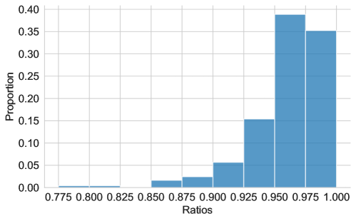
Figure 1: Distribution of ratios, with GILD and GSK as underlying assets.

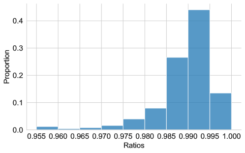
Figure 2: Distribution of ratios, with JPM and MS as underlying assets.

Appendix A Proofs of results

Proof of Proposition 3.3.

Define $f^{h}(x_{1:N}):=\int h_{t}(y_{1:t})\pi(dy_{1:t}|x_{1:N})$ with $h_{t}\in C_{b}({\mathcal{Y}}_{1:t})$. It is worth noting that $f^{h}(x_{1:N})$ is defined $\pi$-almost surely. A coupling $\pi\in\Pi(\bar{\mu},\bar{\nu})$ is causal if and only if

$$f^{h}(x_{1:N})=\int f^{h}(x_{1:t},\bar{x}_{t+1:N})\pi(d\bar{x}_{t+1:N}|x_{1:t}),\quad\pi\text{-a.s.}$$ (A.1)

for all $1\leq t\leq N$ and all $f^{h}$ defined with $h_{t}\in C_{b}({\mathcal{Y}}_{1:t})$. We emphasize that (A.1) holds $\pi$-almost surely, and the conditional kernel $\pi(d\bar{x}_{t+1:N}|x_{1:t})$ depends on the choice of $\pi$ since the joint distribution of $X_{1:N}$ is not fixed.

Furthermore, (A.1) holds if and only if for any $g_{t}\in C_{b}({\mathcal{X}}_{1:N})$, we have

$$\int g_{t}(x_{1:N})\left[f^{h}(x_{1:N})-\int f^{h}(x_{1:t},\bar{x}_{t+1:N})\pi(d\bar{x}_{t+1:N}|x_{1:t})\right]\pi(dx_{1:N})=0.$$ (A.2)

Interchanging the expectations yields

$$\int f^{h}(x_{1:N})\left[g_{t}(x_{1:N})-\int g_{t}(x_{1:t},\bar{x}_{t+1:N})\pi(d\bar{x}_{t+1:N}|x_{1:t})\right]\pi(dx_{1:N})=0.$$ (A.3)

Subsequently, utilizing the tower property, (A.3) is equivalent to

$$\int h_{t}(y_{1:t})\left[g_{t}(x_{1:N})-\int g_{t}(x_{1:t},\bar{x}_{t+1:N})\pi(d\bar{x}_{t+1:N}|x_{1:t})\right]\pi(dx_{1:N},dy_{1:N})=0.$$ (A.4)

∎

Proof of Theorem 4.5.

If we substitute the cost $c$ with $c+C(1+\sum^{N}_{i=1}|x_{i}|+\sum^{N}_{j=1}|y_{j}|)$, it only introduces a finite constant to the original problem, thanks to the finite first moments and marginal conditions. Consequently, we can assume $c\geq 0$ henceforth.

We endow $L^{1}(\mathbb{R}^{N}\times\mathbb{R}^{N})$ with the weak topology, where $f_{n}$ converges to $f$ in the weak topology if and only if

$$\int f_{n}vd\lambda\rightarrow\int fvd\lambda,\quad\forall\,v\in L^{\infty}(\mathbb{R}^{N}\times\mathbb{R}^{N}).$$

The set ${\mathcal{M}}(\bar{g},\bar{h};l,u)$ is uniformly integrable, as every function in this set is bounded by the same integrable function $u$. According to Bogachev, (2007, Theorem 4.7.18), ${\mathcal{M}}(\bar{g},\bar{h};l,u)$ has a compact closure under the weak topology of $L^{1}(\mathbb{R}^{N}\times\mathbb{R}^{N})$. If we can demonstrate that ${\mathcal{M}}(\bar{g},\bar{h};l,u)$ is closed, then it is also compact.

Consider a sequence of functions $\{f_{n}\}$ in ${\mathcal{M}}(\bar{g},\bar{h};l,u)$ that converges to $f$ in the weak topology of $L^{1}(\mathbb{R}^{N}\times\mathbb{R}^{N})$. This convergence is expressed as:

$$\lim_{n\rightarrow\infty}\int f_{n}vd\lambda=\int fvd\lambda.$$

First, select $v=\mathbf{1}_{A}$ with a measurable set $A$ in $\mathbb{R}^{N}\times\mathbb{R}^{N}$. Since it holds that

$$\int f_{n}(x_{1:N},y_{1:N})v(x_{1:N},y_{1:N})d\lambda\leq\int u(x_{1:N},y_{1:N})v(x_{1:N},y_{1:N})d\lambda,$$

we can obtain that $f\leq u$ a.e. Similarly, consider $v(x_{1:N},y_{1:N})=\psi(x_{1})\in L^{\infty}(\mathbb{R})$. Then, $f(x_{1:N},y_{1:N})$ has the marginal $g_{1}$ on $x_{1}$. Other marginal constraints can also be verified. To establish that $f$ satisfies the martingale constraint, we observe that

$$\Big{|}\int_{\mathbb{R}^{N}\times\mathbb{R}^{N}}f_{n}(x_{1:N},y_{1:N})\alpha_{t}(x_{1:t},y_{1:t})(x_{t+1}-x_{t})d\lambda$$

$$\qquad-\int_{\mathbb{R}^{N}\times\mathbb{R}^{N}}f(x_{1:N},y_{1:N})\alpha_{t}(x_{1:t},y_{1:t})(x_{t+1}-x_{t})d\lambda\Big{|}$$

$$\leq\Big{|}\int_{K}f_{n}(x_{1:N},y_{1:N})\alpha_{t}(x_{1:t},y_{1:t})(x_{t+1}-x_{t})d\lambda-\int_{K}f(x_{1:N},y_{1:N})\alpha_{t}(x_{1:t},y_{1:t})(x_{t+1}-x_{t})d\lambda\Big{|}$$

$$\quad+\Big{|}\int_{(\mathbb{R}^{N}\times\mathbb{R}^{N})\backslash K}f_{n}(x_{1:N},y_{1:N})\alpha_{t}(x_{1:t},y_{1:t})(x_{t+1}-x_{t})d\lambda$$

$$\qquad\quad-\int_{(\mathbb{R}^{N}\times\mathbb{R}^{N})\backslash K}f(x_{1:N},y_{1:N})\alpha_{t}(x_{1:t},y_{1:t})(x_{t+1}-x_{t})d\lambda\Big{|},$$

where $K:=[-a,a]^{N}\times[-a,a]^{N}$ is a compact set in $\mathbb{R}^{N}\times\mathbb{R}^{N}$, and $\alpha_{t}\in L^{\infty}$. With a given compact set $K$, the first term converges to zero since $x_{t}$ and $x_{t+1}$ are bounded on $K$. The second term is bounded by $\|\alpha_{t}\|_{\infty}\varepsilon$ since $f_{n}$ and $f$ have marginals $(\bar{g},\bar{h})$ with finite first moments. When the side width $a\rightarrow\infty$, we have $\varepsilon\rightarrow 0$. Consequently, $f$ also satisfies the martingale constraint. In summary, the limit $f\in{\mathcal{M}}(\bar{g},\bar{h};l,u)$, and the compactness follows.

The proof of the lower semicontinuity for the objective is standard. When $c$ is bounded, the functional

$$f\mapsto\int cfd\lambda$$

is a continuous, following from the definition of weak topology. In the case where $c$ is nonnegative but unbounded, there exists a sequence of bounded measurable functions $\{c_{n}\}$ converging increasingly to $c$. Using the monotone convergence theorem, we have

$$\int fcd\lambda=\int f\sup_{n}c_{n}d\lambda=\sup_{n}\int fc_{n}d\lambda,$$

demonstrating that $\int fcd\lambda$ is a supremum of continuous functionals and, consequently, l.s.c. The claim then follows as the infimum is attained for an l.s.c. functional on a compact set. ∎

Proof of Lemma 4.6.

Similarly to the proof of Villani, (2003, Proposition 1.22), we can substitute the cost $c$ for $c+C(1+|x|+|y|)+\varepsilon$ for an arbitrarily large $\varepsilon>0$. With the finite first moments and marginal conditions, this modification adds the same finite constant to both sides of the strong duality. The result for the modified cost implies the result for the original cost function $c$. Hence, we proceed with the assumption $c\geq\varepsilon>0$ in the subsequent analysis.

Define the functionals $\Xi$ and $\Theta$ as follows:

$$\Xi: (b(x,y),\kappa(x,y))\in C_{b}(\mathbb{R}\times\mathbb{R})\times C_{b}(\mathbb{R}\times\mathbb{R})$$ (A.5)

$$\mapsto\left\{\begin{array}[]{lll}&\int\phi(x)g(x)dx+\int\varphi(y)h(y)dy-\int\kappa(x,y)u(x,y)dxdy,\\ &\text{ if }b(x,y)=\phi(x)+\varphi(y)\text{ and }\kappa(x,y)\leq 0;\\ &+\infty,\text{ else. }\\ \end{array}\right.$$

and

$$\Theta: (b(x,y),\kappa(x,y))\in C_{b}(\mathbb{R}\times\mathbb{R})\times C_{b}(\mathbb{R}\times\mathbb{R})$$ (A.6)

$$\mapsto\left\{\begin{array}[]{lll}&0,\text{ if }b(x,y)\geq-c(x,y)+\kappa(x,y)\text{ and }\kappa(x,y)\leq 0;\\ &+\infty,\text{ else. }\\ \end{array}\right.$$

$\Xi$ is well-defined. Specifically, if $\phi(x)+\varphi(y)=\tilde{\phi}(x)+\tilde{\varphi}(y)$ for all $x$ and $y$, then $\phi=\tilde{\phi}+s$ and $\varphi=\tilde{\varphi}-s$ with a constant $s$; see Villani, (2003, Section 1.1, p.27) for the same argument. Analogously, $\Theta$ is also well-defined.

To verify the assumptions in Fenchel-Rockafellar duality theorem (Villani,, 2003, Theorem 1.9), we observe that $\Xi$ and $\Theta$ are finite at $(b,\kappa)=(0,-1)$. Moreover, under conditions $\|b\|_{\infty}\leq\varepsilon$ and $\|\kappa+1\|_{\infty}\leq\frac{1}{2}$, it follows that $\kappa\leq 0$ and $-c+\kappa\leq-\varepsilon\leq b$. Consequently, $\Theta(0,-1)=0$, and therefore $\Theta$ is continuous at $(0,-1)$.

A direct calculation yields

$$\inf_{(b,\kappa)\in C_{b}\times C_{b}}\Big{[}\Theta(b,\kappa)+\Xi(b,\kappa)\Big{]}$$

$$=\inf_{(\phi,\varphi,\kappa)\in C_{b}\times C_{b}\times C_{b}}\Big{[}\int\phi(x)g(x)dx+\int\varphi(y)h(y)dy-\int\kappa(x,y)u(x,y)dxdy\Big{|}$$

$$\hskip 113.81102pt\phi(x)+\varphi(y)\geq-c(x,y)+\kappa(x,y),\kappa\leq 0\Big{]}$$

$$=-\sup_{(\phi,\varphi,\kappa)\in C_{b}\times C_{b}\times C_{b}}\Big{[}\int\phi(x)g(x)dx+\int\varphi(y)h(y)dy-\int\kappa(x,y)u(x,y)dxdy\Big{|}$$

$$\hskip 113.81102pt\phi(x)+\varphi(y)\leq c(x,y)+\kappa(x,y),\kappa\geq 0\Big{]},$$

where in the last equality, we substitute $(\phi,\varphi,\kappa)$ with $(-\phi,-\varphi,-\kappa)$.

A challenge arises due to the fact that the topological dual of $C_{b}(\mathbb{R}\times\mathbb{R})$, denoted as $(C_{b}(\mathbb{R}\times\mathbb{R}))^{*}$, is greater than $M(\mathbb{R}\times\mathbb{R})$, which represents the set of all finite signed measures. To calculate the Legendre-Fenchel transforms of $\Theta$ and $\Xi$, we take advantage of Villani, (2003, Lemmas 1.24 and 1.25) to deal with continuous linear functionals on $C_{b}(\mathbb{R}\times\mathbb{R})$. In addition, we note that the topological dual of the product space $C_{b}(\mathbb{R}\times\mathbb{R})\times C_{b}(\mathbb{R}\times\mathbb{R})$ is the product of dual spaces, namely $(C_{b}(\mathbb{R}\times\mathbb{R}))^{*}\times(C_{b}(\mathbb{R}\times\mathbb{R}))^{*}$.

With linear forms $(l_{1},l_{2})\in(C_{b}(\mathbb{R}\times\mathbb{R}))^{*}\times(C_{b}(\mathbb{R}\times\mathbb{R}))^{*}$, the Legendre-Fenchel transform of $\Theta$ is defined as follows:

$$\Theta^{*}(-l_{1},-l_{2})$$

$$=\sup_{(b,\kappa)\in C_{b}\times C_{b}}\Big{[}\left\langle-l_{1},b\right\rangle+\left\langle-l_{2},\kappa\right\rangle\Big{|}b(x,y)\geq-c(x,y)+\kappa(x,y),\;\kappa(x,y)\leq 0\Big{]}$$

$$=\sup_{(b,\kappa)\in C_{b}\times C_{b}}\Big{[}\left\langle l_{1},b-\kappa\right\rangle+\left\langle l_{1}+l_{2},\kappa\right\rangle\Big{|}b(x,y)\leq c(x,y)+\kappa(x,y),\;\kappa(x,y)\geq 0\Big{]},$$

where $\left\langle\cdot,\cdot\right\rangle$ denotes the duality bracket (Villani,, 2003, p. xiv).

If there exists $v\geq 0$ satisfying $\left\langle l_{1}+l_{2},v\right\rangle>0$, then we can choose $b=\kappa=kv$ and send $k\rightarrow\infty$. Similarly, if there exist $v\geq 0$ and $\left\langle l_{1},v\right\rangle<0$, then we can consider $\kappa=0$ and $b=-kv$ with $k\rightarrow\infty$. Therefore, $\Theta^{*}(-l_{1},-l_{2})<+\infty$ only when $l_{1}$ is nonnegative and $l_{1}+l_{2}$ is nonpositive.

Furthermore, the Legendre-Fenchel transform of $\Xi$ is given by

$$\Xi^{*}(l_{1},l_{2})=\sup_{(b,\kappa)\in C_{b}\times C_{b}}\Big{[} \left\langle l_{1},b\right\rangle+\left\langle l_{2},\kappa\right\rangle-\int\phi(x)g(x)dx-\int\varphi(y)h(y)dy$$

$$+\int\kappa(x,y)u(x,y)dxdy\Big{|}b(x,y)=\phi(x)+\varphi(y)\text{ and }\kappa(x,y)\leq 0\Big{]}.$$

To avoid $\Xi^{*}(l_{1},l_{2})=+\infty$, we first need

$$\left\langle l_{1},\phi+\varphi\right\rangle=\int\phi(x)g(x)dx+\int\varphi(y)h(y)dy.$$ (A.7)

It is noteworthy that $l_{1}$ should be nonnegative, as argued above. Moreover, $l_{1}$ also acts continuously on the subset $C_{0}(\mathbb{R}\times\mathbb{R})$ of $C_{b}(\mathbb{R}\times\mathbb{R})$, where $C_{0}(\mathbb{R}\times\mathbb{R})$ denotes the set of all continuous functions approaching 0 at infinity. Since the topological dual of $C_{0}(\mathbb{R}\times\mathbb{R})$ is $M(\mathbb{R}\times\mathbb{R})$, there exists a unique measure $\pi\in M(\mathbb{R}\times\mathbb{R})$ such that

$$\left\langle l_{1},v\right\rangle=\int v(x,y)d\pi,\quad\forall\,v\in C_{0}(\mathbb{R}\times\mathbb{R}).$$

We can then decompose $l_{1}=\pi+R$, where $R$ is a continuous linear functional with

$$\left\langle R,v\right\rangle=0,\quad\forall\,v\in C_{0}(\mathbb{R}\times\mathbb{R}).$$

Under the condition (A.7), Villani, (2003, Lemma 1.25) shows that $R=0$, and $l_{1}=\pi$ is a nonnegative measure with Borel marginals $gdx$ and $hdy$.

Another requirement to avoid $\Xi^{*}(l_{1},l_{2})=+\infty$ is

$$\left\langle l_{2},\kappa\right\rangle+\int\kappa(x,y)u(x,y)dxdy\leq 0,\quad\forall\,\kappa(x,y)\leq 0,\,\kappa\in C_{b}(\mathbb{R}\times\mathbb{R}).$$ (A.8)

Since $l_{1}+l_{2}$ is nonpositive and $l_{1}$ is a measure, then

$$\left\langle l_{1}+l_{2},v\right\rangle=\int v(x,y)d\pi+\left\langle l_{2},v\right\rangle\leq 0,\quad\forall\,v(x,y)\geq 0,\,v\in C_{b}(\mathbb{R}\times\mathbb{R}).$$ (A.9)

Together with (A.8), setting $\kappa=-v$ yields

$$\int v(x,y)d\pi\leq-\left\langle l_{2},v\right\rangle\leq\int v(x,y)u(x,y)dxdy,\quad\forall\,v(x,y)\geq 0,\,v\in C_{b}(\mathbb{R}\times\mathbb{R}).$$ (A.10)

This implies that $\pi$ is absolutely continuous with respect to the Lebesgue measure $\lambda$ on the Borel $\sigma$-algebra of $\mathbb{R}\times\mathbb{R}$. Otherwise, suppose that the opposite is true. Then, there exists a Borel set $B$ such that $\lambda(B)=0$ and $\pi(B)>0$. Since $\pi$ is regular (Bertsekas and Shreve,, 1978, Proposition 7.17), there exists a closed subset $F\subset B$ and $\pi(F)>\delta>0$ for a small $\delta$. Similar to the proof of Bertsekas and Shreve, (1978, Proposition 7.18), let $G_{n}=\{(x,y)\in\mathbb{R}\times\mathbb{R}|d((x,y),F)<1/n\}$ with a sufficiently large $n$. By Urysohn’s lemma, there exist continuous functions $0\leq v_{n}\leq 1$ such that $v_{n}=0$ on $G^{c}_{n}$ and $v_{n}=1$ on $F$. Then

$$\pi(F)\leq\int v_{n}(x,y)d\pi\leq\int v_{n}(x,y)u(x,y)d\lambda\leq\|u\|_{\infty}\int v_{n}d\lambda\leq\|u\|_{\infty}\lambda(G_{n}),$$

which implies

$$\pi(F)\leq\|u\|_{\infty}\lambda(\cap^{\infty}_{n=1}G_{n})=\|u\|_{\infty}\lambda(F)\leq\|u\|_{\infty}\lambda(B)=0,$$

leading to a contradiction with $\pi(F)>\delta>0$. By the Radon-Nikodým theorem (Rogers and Williams,, 1993, Theorem 9.3, p.98), the Radon-Nikodým density exists: $f(x,y)=\frac{d\pi}{d\lambda},\,\lambda\text{-a.e.}$

Furthermore, (A.10) implies $f(x,y)\leq u(x,y),\,\lambda\text{-a.e.}$ Otherwise, suppose $\lambda(B)>0$, where $B:=\{(x,y)\in\mathbb{R}\times\mathbb{R}|f(x,y)>u(x,y)\}$. $B$ is a Borel set. Since $\lambda$ is regular, there exists a closed subset $F\subset B$ and $\lambda(F)>0$. Introducing continuous and bounded functions $v_{n}$ similarly as before, (A.10) and the dominated convergence theorem lead to

$$\int\textbf{1}_{F}fd\lambda\leq\int v_{n}fd\lambda\leq\int v_{n}ud\lambda\leq\int\textbf{1}_{G_{n}}ud\lambda\rightarrow\int\textbf{1}_{F}ud\lambda,$$

which contradicts the fact that $f>u$ on $F$ and $\lambda(F)>0$.

In summary, $\Theta^{*}(-l_{1},-l_{2})+\Xi^{*}(l_{1},l_{2})<+\infty$ requires that $l_{1}$ is a probability measure in $\Pi(g,h)$ with density $0\leq f\leq u$ and $l_{1}+l_{2}$ is nonpositive. When these conditions are satisfied, it follows that $\Xi^{*}(l_{1},l_{2})=0$ and

$$\Theta^{*}(-l_{1},-l_{2}) =\sup_{b\in C_{b}}\Big{[}\int b(x,y)f(x,y)dxdy\Big{|}b(x,y)\leq c(x,y)\Big{]}=\int c(x,y)f(x,y)dxdy,$$

because the l.s.c. cost $c\geq\varepsilon$ can be approximated pointwise by a monotonically increasing sequence of continuous and bounded functions. Then the equality above follows from the monotone convergence theorem. Therefore, the right-hand side of the Fenchel-Rockafellar duality reduces to

$$\max_{(l_{1},l_{2})\in(C_{b})^{*}\times(C_{b})^{*}}\Big{[}-\Theta^{*}(-l_{1},-l_{2})-\Xi^{*}(l_{1},l_{2})\Big{]} =-\min_{f\in\Pi(g,h;u)}\int c(x,y)f(x,y)dxdy.$$

We have proved the strong duality (4.20), albeit with continuous and bounded $(\phi,\varphi,\kappa)$. In the $L^{1}$ case, the claim follows from

$$\inf_{f\in\Pi(g,h;u)}P(f)=\sup_{\Psi_{c}\cap C_{b}}F(\phi,\varphi,\kappa)\leq\sup_{\Psi_{c}}F(\phi,\varphi,\kappa)\leq\inf_{f\in\Pi(g,h;u)}P(f),$$

where the last inequality is a result of weak duality, similar to Villani, (2003, Proposition 1.5). In addition, in the first equality, the notation $\Psi_{c}\cap C_{b}$ indicates that $(\phi,\varphi,\kappa)$ are also continuous and bounded. ∎

Proof of Theorem 4.7.

Similarly to the proof of Lemma 4.6, we can assume the cost $c\geq 0$.

Consider a continuous and bounded cost $c$. Maximization in the dual problem can be achieved in two steps. First, we maximize over $(\phi,\varphi,\kappa)$ when other multipliers $(\alpha,\beta,\gamma,\eta,\theta)$ are given. This reduces to a dual problem with the upper capacity constraint in Lemma 4.6, but with a new cost given by

$$\tilde{c}(x_{1:N},y_{1:N},\alpha,\beta,\gamma,\eta,\theta;u,l)$$ (A.11)

$$=c(x_{1:N},y_{1:N})-\theta(x_{1:N},y_{1:N})$$

$$\quad+\sum^{N-1}_{t=1}\alpha_{t}(x_{1:t},y_{1:t})(x_{t+1}-x_{t})+\sum^{N-1}_{t=1}\beta_{t}(x_{1:t},y_{1:t})(y_{t+1}-y_{t})$$

$$\quad+\Psi(x_{1:N},y_{1:N},\gamma,\eta;u,l).$$

On the basis of our assumptions, we have $c,\theta,\alpha,\beta,\gamma,\eta,u,l\in C_{b}$. Hence, $\tilde{c}$ is continuous, and $|\tilde{c}|\leq C(1+\sum^{N}_{t=1}|x_{t}|+\sum^{N}_{t=1}|y_{t}|)$. An application of Lemma 4.6 leads to

$$D =\sup_{\begin{subarray}{c}\alpha_{t},\beta_{t}\\ \gamma_{t,i},\,\eta_{t,i}\geq 0\\ \theta\geq 0\end{subarray}}\sup_{\begin{subarray}{c}\Phi_{c}\text{ with }(\alpha_{t},\beta_{t},\gamma_{t,i},\,\eta_{t,i},\theta)\text{ given }\end{subarray}}D(\phi,\varphi,\alpha,\beta,\gamma,\eta,\kappa,\theta)$$ (A.12)

$$=\sup_{\begin{subarray}{c}\alpha_{t},\beta_{t}\\ \gamma_{t,i},\,\eta_{t,i}\geq 0\\ \theta\geq 0\end{subarray}}\inf_{f\in\Pi(\bar{g},\bar{h};u)}\int\tilde{c}(x_{1:N},y_{1:N},\alpha,\beta,\gamma,\eta,\theta;u,l)f(x_{1:N},y_{1:N})d\lambda$$ (A.13)

$$=\inf_{f\in\Pi(\bar{g},\bar{h};u)}\sup_{\begin{subarray}{c}\alpha_{t},\beta_{t}\\ \gamma_{t,i},\,\eta_{t,i}\geq 0\\ \theta\geq 0\end{subarray}}\int\tilde{c}(x_{1:N},y_{1:N},\alpha,\beta,\gamma,\eta,\theta;u,l)f(x_{1:N},y_{1:N})d\lambda$$ (A.14)

$$=\inf_{f\in{\mathcal{M}}(\bar{g},\bar{h};l,u)}\int c(x_{1:N},y_{1:N})f(x_{1:N},y_{1:N})d\lambda=P.$$ (A.15)

(A.14) follows from the minimax theorem, given in Strasser, (1985, Theorem 45.8, p. 239) or Beiglböck et al., (2013, Theorem 3.1). In fact, $\Pi(\bar{g},\bar{h};u)$ is compact in the weak topology of $L^{1}$. Since $\tilde{c}$ has a linear growth rate and the marginals have finite first moments, we can also prove that the objective $\int\tilde{c}fd\lambda$ is continuous in $f\in\Pi(\bar{g},\bar{h};u)$ using the weak topology of $L^{1}$, similar to the approach in Beiglböck et al., (2013, Lemma 2.2).

The final equality (A.15) is derived from the observation that any violation of the martingale condition, the McCormick relaxations, or the lower bound results in an infinite value.

In the case of a nonnegative and l.s.c. cost function $c$, the strong duality can be established through a standard approximation argument. For example, see the last part of the proof presented in Beiglböck et al., (2013, Theorem 1.1). ∎

References

- Acciaio et al., (2021) Acciaio, B., Backhoff-Veraguas, J., and Jia, J. (2021). Cournot–Nash equilibrium and optimal transport in a dynamic setting. SIAM Journal on Control and Optimization, 59(3):2273–2300.
- Acciaio et al., (2020) Acciaio, B., Backhoff-Veraguas, J., and Zalashko, A. (2020). Causal optimal transport and its links to enlargement of filtrations and continuous-time stochastic optimization. Stochastic Processes and their Applications, 130(5):2918–2953.
- Alfonsi et al., (2017) Alfonsi, A., Corbetta, J., and Jourdain, B. (2017). Sampling of probability measures in the convex order and approximation of martingale optimal transport problems. Available at SSRN 3072356.
- Anstreicher, (2009) Anstreicher, K. M. (2009). Semidefinite programming versus the reformulation-linearization technique for nonconvex quadratically constrained quadratic programming. Journal of Global Optimization, 43:471–484.
- Audet et al., (2000) Audet, C., Hansen, P., Jaumard, B., and Savard, G. (2000). A branch and cut algorithm for nonconvex quadratically constrained quadratic programming. Mathematical Programming, 87:131–152.
- Backhoff-Veraguas et al., (2020) Backhoff-Veraguas, J., Bartl, D., Beiglböck, M., and Eder, M. (2020). Adapted Wasserstein distances and stability in mathematical finance. Finance and Stochastics, 24(3):601–632.
- Backhoff-Veraguas et al., (2017) Backhoff-Veraguas, J., Beiglböck, M., Lin, Y., and Zalashko, A. (2017). Causal transport in discrete time and applications. SIAM Journal on Optimization, 27(4):2528–2562.
- Backhoff-Veraguas and Pammer, (2022) Backhoff-Veraguas, J. and Pammer, G. (2022). Stability of martingale optimal transport and weak optimal transport. The Annals of Applied Probability, 32(1):721–752.
- Backhoff-Veraguas and Zhang, (2023) Backhoff-Veraguas, J. and Zhang, X. (2023). Dynamic Cournot-Nash equilibrium: the non-potential case. Mathematics and Financial Economics, 17(2):153–174.
- Bayraktar et al., (2021) Bayraktar, E., Zhang, X., and Zhou, Z. (2021). Transport plans with domain constraints. Applied Mathematics & Optimization, 84(1):1131–1158.
- Beiglböck et al., (2013) Beiglböck, M., Henry-Labordere, P., and Penkner, F. (2013). Model-independent bounds for option prices – a mass transport approach. Finance and Stochastics, 17:477–501.
- Beiglböck and Juillet, (2016) Beiglböck, M. and Juillet, N. (2016). On a problem of optimal transport under marginal martingale constraints. Annals of Probability, 44(1):42–106.
- Beiglböck et al., (2019) Beiglböck, M., Lim, T., and Obłój, J. (2019). Dual attainment for the martingale transport problem. Bernoulli, 25(3):1640–1658.
- Beiglböck et al., (2017) Beiglböck, M., Nutz, M., and Touzi, N. (2017). Complete duality for martingale optimal transport on the line. The Annals of Probability, 45(5):3038–3074.
- Bertsekas and Shreve, (1978) Bertsekas, D. and Shreve, S. E. (1978). Stochastic optimal control: The discrete-time case. Academic Press.
- Bogachev, (2007) Bogachev, V. I. (2007). Measure Theory, volume II. Springer Science & Business Media.
- Bogachev, (2022) Bogachev, V. I. (2022). Kantorovich problems with a parameter and density constraints. Siberian Mathematical Journal, 63(1):34–47.
- Breeden and Litzenberger, (1978) Breeden, D. T. and Litzenberger, R. H. (1978). Prices of state-contingent claims implicit in option prices. Journal of Business, pages 621–651.
- Brückerhoff and Juillet, (2022) Brückerhoff, M. and Juillet, N. (2022). Instability of martingale optimal transport in dimension . Electronic Communications in Probability, 27(none):1 – 10.
- Davis and Hobson, (2007) Davis, M. H. and Hobson, D. G. (2007). The range of traded option prices. Mathematical Finance, 17(1):1–14.
- De Marco and Henry-Labordere, (2015) De Marco, S. and Henry-Labordere, P. (2015). Linking vanillas and VIX options: A constrained martingale optimal transport problem. SIAM Journal on Financial Mathematics, 6(1):1171–1194.
- Eckstein et al., (2021) Eckstein, S., Guo, G., Lim, T., and Obłój, J. (2021). Robust pricing and hedging of options on multiple assets and its numerics. SIAM Journal on Financial Mathematics, 12(1):158–188.
- Fahim and Huang, (2016) Fahim, A. and Huang, Y.-J. (2016). Model-independent superhedging under portfolio constraints. Finance and Stochastics, 20:51–81.
- Fengler, (2009) Fengler, M. R. (2009). Arbitrage-free smoothing of the implied volatility surface. Quantitative Finance, 9(4):417–428.
- Guo and Obłój, (2019) Guo, G. and Obłój, J. (2019). Computational methods for martingale optimal transport problems. The Annals of Applied Probability, 29(6):3311–3347.
- Guyon et al., (2017) Guyon, J., Menegaux, R., and Nutz, M. (2017). Bounds for VIX futures given S&P 500 smiles. Finance and Stochastics, 21:593–630.
- Hobson and Neuberger, (2012) Hobson, D. and Neuberger, A. (2012). Robust bounds for forward start options. Mathematical Finance, 22(1):31–56.
- Kallenberg, (2021) Kallenberg, O. (2021). Foundations of Modern Probability. Springer Science & Business Media. The third edition.
- Korman and McCann, (2015) Korman, J. and McCann, R. (2015). Optimal transportation with capacity constraints. Transactions of the American Mathematical Society, 367(3):1501–1521.
- Korman et al., (2015) Korman, J., McCann, R. J., and Seis, C. (2015). An elementary approach to linear programming duality with application to capacity constrained transport. Journal of Convex Analysis, 22(3):797–808.
- Lassalle, (2013) Lassalle, R. (2013). Causal transference plans and their Monge-Kantorovich problems. arXiv preprint arXiv:1303.6925.
- Lütkebohmert and Sester, (2019) Lütkebohmert, E. and Sester, J. (2019). Tightening robust price bounds for exotic derivatives. Quantitative Finance, 19(11):1797–1815.
- McCormick, (1976) McCormick, G. P. (1976). Computability of global solutions to factorable nonconvex programs: Part I – Convex underestimating problems. Mathematical Programming, 10(1):147–175.
- Pflug and Pichler, (2012) Pflug, G. C. and Pichler, A. (2012). A distance for multistage stochastic optimization models. SIAM Journal on Optimization, 22(1):1–23.
- Pflug and Pichler, (2014) Pflug, G. C. and Pichler, A. (2014). Multistage stochastic optimization, volume 1104. Springer.
- Rogers and Williams, (1993) Rogers, L. and Williams, D. (1993). Diffusions, Markov Processes, and Martingales: Volume 1, Foundations. Cambridge University Press.
- Sherali and Fraticelli, (2002) Sherali, H. D. and Fraticelli, B. M. (2002). Enhancing RLT relaxations via a new class of semidefinite cuts. Journal of Global Optimization, 22:233–261.
- Strassen, (1965) Strassen, V. (1965). The existence of probability measures with given marginals. The Annals of Mathematical Statistics, 36(2):423–439.
- Strasser, (1985) Strasser, H. (1985). Mathematical theory of statistics: Statistical experiments and asymptotic decision theory, volume 7. Walter de Gruyter.
- Villani, (2003) Villani, C. (2003). Topics in Optimal Transportation. Number 58. American Mathematical Society.
- Wiesel, (2023) Wiesel, J. (2023). Continuity of the martingale optimal transport problem on the real line. The Annals of Applied Probability, 33(6A):4645–4692.