Constant-roll inflation and primordial black holes with Barrow holographic dark energy

Abstract

We investigate the constant-roll inflation and the evolution of primordial black holes (PBHs) with Barrow holographic dark energy (BHDE). Using the modified Friedmann equation and the constant-roll condition in BHDE model, we calculate the constant-roll parameters, the scalar spectral index parameter and the tensor-to-scalar ratio with the chaotic potential $V_{0}\phi^{n}$. Then, we show that a suitable value of the power exponent is $n=1$ by using the Planck 2018 data. Considering the accretion process and the evaporation due to Hawking radiation, we discuss the evolution of PBHs in BHDE model and obtain that the PBHs mass is in the mass window of PBHs.

I Introduction

Inflation, a short period of an exponential accelerating expansion before the radiation dominated era, is the currently widely accepted paradigm of modern cosmology Guth1981 ; Linde1982 . The inflation not only addresses the puzzles of the standard hot Big Bang cosmology but also provides an explanation for the quantum origin of the Cosmic Microwave Background temperature anisotropies and the Large-Scale Structure Mukhanov1981 ; Lewis2000 ; Bernardeau2002 . In general, a scalar field named as the inflaton field drives the exponential accelerating expansion of the universe during the inflationary epoch. The mechanism of inflation is based on the generation of small quantum fluctuations in the inflaton field. The small quantum fluctuations are amplified in physical scale during the inflationary epoch and lead to a Gaussian, scale-invariant and adiabatic primordial density perturbations Weinberg2008 . This information is encoded into the primordial scalar power spectrum described by the scalar spectral index $n_{s}$, which is constrained by the Planck 2018 results Planck2020 . In addition, inflation also predicts the generation of tensor perturbations as primordial gravitational waves described by the tensor-to-scalar ratio $r$ Maggiore2018 . Usually, the dynamics of inflation is based on the slow-roll approximation, in which the scalar potential is chosen to be nearly flat so that the scalar field can slowly roll down this potential. Once the minimum value of this potential is reached, inflation ends. This scenario is called slow-roll inflation Linde1982 ; Noh2001 ; Weinberg2008 , which can be measured by the parameters $\epsilon_{1}=-\dot{H}/H^{2}$ and $\epsilon_{2}=\ddot{\phi}/H\dot{\phi}$. For the slow-roll inflation, the small values of the parameters $\epsilon_{1}\ll 1$ and $\epsilon_{2}\ll 1$ are required. If the scalar potential is assumed to be extremely flat, the second condition becomes $\epsilon_{2}=-3$ which corresponds to the ultra slow-roll condition Martin2013 ; Dimopoulos2017 ; Pattison2018 . In the ultra slow-roll inflation, the curvature perturbations are not frozen at the super Hubble scales thus leading to non-Gaussianities. Furthermore, when the second condition $\epsilon_{2}$ is generalized to be constant, a more generalized scenario named as constant-roll inflation was proposed Motohashi2015 ; Gao2017 ; Gao2018 ; Yi2018 ; Anguelova2018 ; Cicciarella2018 ; Guerrero2020 , in which the rate of acceleration and velocity of the inflaton field are constants. The constant-roll inflation has novel dynamical features enriching physics, which is different from the slow-roll inflation. When the constant-roll inflation was proposed, it drawed widespread attention and was widely studied in lots of theories, such as $f(R)$ gravity Nojiri2017a ; Motohashi2017 , $f(R,\phi)$ gravity Panda2023 , $f(Q,T)$ gravity Bourakadi2023 , scalar-tensor gravity Motohashi2019 , brane gravity Mohammadi2020 , Dirac-Born-Infeld theory Lahiri2022 , Galilean model Herrera2023 , holographic dark energy Mohammadi2022 , Tsallis holographic dark energy Keskin2023 , and so on.

After inflation ended, the primordial inhomogeneities of the primordial power spectrum on small scales re-entered the Hubble horizon in the radiation dominated era, significant amount of primordial black holes (PBHs) can be formed as a result of the gravitational collapse Hawking1971 ; Carr1974 if the amplitude of the primordial power spectrum produced during inflation is strong enough. After PBHs were proposed, they were found that they could be a candidate of dark matter Chapline1975 and were reconsidered Bird2016 ; Sasaki2016 after black holes mergers were detected by LIGO Abbott2016 . PBHs can offer us an opportunity to explore the physics of the early universe and may play some important roles in cosmology. Thus, PBHs were widely discussed in some modified gravity theories, such as scalar-tensor gravity Barrow1996 , $f(T)$ gravity Bhadra2013 , Brans-Dicke gravity Aliferis2021 , $f(Q)$ gravity Chanda2022 , teleparallel gravity Bourakadi2022 , $f(Q,T)$ gravity Bourakadi2023 , and studied in some inflationary models including slow-roll inflation Carr1993 ; Ivanov1994 ; Yokoyama1998 ; Bellido2017 ; Biagetti2018 ; Fu2020 ; Davies2022 , ultra-slow-roll inflation Di2018 ; Fu2019 ; Ballesteros2020 ; Liu2021 ; Figueroa2022 and constant-roll inflation Motohashi2020 ; Tomberg2023 ; Bourakadi2023 . PBHs also have attracted lots of attention since they may constitute part or all of dark matter Clesse2015 ; Kawasaki2016 ; Carr2016 ; Inomata2017 ; Inomata2018 ; Carr2018 ; Germani2019 ; Kusenko2020 ; Pacheco2020 ; Calabrese2022 ; Pacheco2023 ; Flores2023 ; Dike2023 , they may play a role in the synthesis of heavy elements Fuller2017 ; Keith2020 and could be responsible for some astrophysical phenomena, such as, seeding supermassive black holes Kawasaki2012 ; Clesse2015 ; Carr2018 ; Kusenko2020 , seeding galaxies Clesse2015 ; Carr2018 , explaining the gravitational wave signals observed by the LIGO detectors Inomata2017a ; Kusenko2020 . The existence of PBHs formed in the early universe still remains an open question. PBHs with mass smaller than $5\times 10^{11}kg$ would have been evaporated by Hawking radiation now Page1976 . When PBHs are considered as dark matter, the currently allowed mass window for PBHs was shown around $10^{20}g$ Inomata2017 , $10^{-10}-10^{-8}M_{\odot}$ Kuhnel2017 , $5\times 10^{-16}M_{\odot}$, $2\times 10^{-14}M_{\odot}$ and $25-100M_{\odot}$ Carr2017 , $10^{16}-10^{17}g$, $10^{20}-10^{24}g$ and $1-10^{3}M_{\odot}$ Carr2016 , $10^{4}-10^{6}M_{\odot}$ Dike2023 , $10^{6}-10^{12}M_{\odot}$ DAgostino2023 , so the allowed mass window for PBHs is seemingly broad and a more accurate mass window needs further investigation.

The holographic dark energy is one competitive candidates of dark energy Hsu2004 ; Horvat2004 ; Li2004 , which is used to explain the late time acceleration of the universe, and is proposed based on the holographic principle stating that the entropy of a system is scaled on its surface area Witten1998 ; Bousso2002 . The cornerstone of holographic dark energy is the horizon entropy, and different horizon entropy will result in different holographic dark energy models. Recently, combining the holographic principle and Barrow entropy Barrow2020a , Barrow holographic dark energy(BHDE) with different IR cutoff was proposed Saridakis2020 ; Anagnostopoulos2020a ; Srivastava2021a ; Sheykhi2021 ; Oliveros2022 and subsequently widely studied in theories Huang2021 ; Adhikary2021 ; Mamon2021 ; Rani2021 ; Luciano2022 ; Nojiri2022 ; Paul2022 ; Luciano2023 ; Boulkaboul2023 ; Pankaj2023 ; Ghaffari2023 and observations Asghari2022 ; Jusufi2022 ; Barrow2021 ; Anagnostopoulos2020 .

Recently, the constant-roll inflation was studied in holographic dark energy model Mohammadi2022 and Tsallis holographic dark energy model Keskin2023 , the results show that the constant-roll inflation can be realized in these models under some conditions. So, whether the constant-roll inflation can also be realized in BHDE model. This is the main goal of this paper. Then, the evolution of PBHs, which is formed after inflation ended, is analyzed. The paper is organized as follows. In section II, we briefly review the modified Friedmann equation in BHDE model. In section III, we study the constant-roll inflation in BHDE model. In section IV, we analyze the evolution of PBHs in BHDE model. Finally, our main conclusions are shown in Section V.

II Modified Friedmann Equations

In a homogeneous and isotropic Friedmann-Robertson-Walker universe described by the Friedmann-Lema$\hat{i}$tre-Robertson-Walker metric

$$ds^{2}=-dt^{2}+a(t)^{2}\gamma_{ij}dx^{i}dx^{j},$$ (1)

where $a(t)$ denotes the scale factor, and $\gamma_{ij}$ represents the metric on the three-sphere

$$\gamma_{ij}dx^{i}dx^{j}=\frac{dr^{2}}{1-Kr^{2}}+r^{2}(d\theta^{2}+\sin^{2}\theta d\phi^{2}).$$ (2)

Here, $K$ is the spatial curvature. Considering the apparent horizon as the IR cutoff, the Friedmann equation in BHDE model can be modified as Sheykhi2021

$$\Big{(}H^{2}+\frac{K}{a^{2}}\Big{)}^{1-\frac{\delta}{2}}=\frac{8\pi G_{eff}}{3}\rho_{\phi},$$ (3)

where $\delta$ satisfies the relation $0\leq\delta\leq 1$ and stands for the amount of the quantum-gravitational deformation effects Barrow2020 , $\delta=0$ represents the standard holographic dark energy and $\delta=1$ denotes the most intricate and fractal structure of the horizon, and $G_{eff}$ represents the effective Newtonian gravitational constant as

$$G_{eff}=\frac{A_{0}}{4}\Big{(}\frac{2-\delta}{2+\delta}\Big{)}\Big{(}\frac{A_{0}}{4\pi}\Big{)}^{\frac{\delta}{2}}.$$ (4)

In the case $\delta\rightarrow 0$, the area law of entropy is recovered, and we have $A_{0}\rightarrow 4G$. As a result, $G_{eff}\rightarrow G$ and the standard Friedmann equation is obtained.

We consider the matter contents of the early universe as a scalar field, and the energy density and the pressure take the form

$$\rho_{\phi}=\frac{1}{2}\dot{\phi}^{2}+V(\phi),\qquad p_{\phi}=\frac{1}{2}\dot{\phi}^{2}-V(\phi),$$ (5)

which satisfies the continuity equation

$$\dot{\rho}_{\phi}+3H(\rho_{\phi}+p_{\phi})=0.$$ (6)

It can be written as the Klein-Gordon equation

$$\ddot{\phi}+3H\dot{\phi}+V_{\phi}=0.$$ (7)

Combing Eqs. (3) and  (6), the second Friedmann equation can be derived as Sheykhi2021

$$(2-\delta)\Big{(}1+\frac{\dot{H}}{H^{2}}\Big{)}\Big{(}H^{2}+\frac{k}{a^{2}}\Big{)}^{-\frac{\delta}{2}}H^{2}+(1+\delta)\Big{(}H^{2}+\frac{k}{a^{2}}\Big{)}^{1-\frac{\delta}{2}}=-8\pi G_{eff}p_{\phi}.$$ (8)

III Constant-roll Inflation

In this section, we will discuss the constant-roll condition on the Friedmann equations given by Eqs. (3) and  (8) in a flat universe. During inflation, the universe is characterized by the scalar spectral index parameter $n_{s}$ and the tensor-to-scalar ratio $r$ which are given by Nojiri2017 ; Hwang2005

$$n_{s}\simeq 1-4\epsilon_{1}-2\epsilon_{2},\qquad r=16\epsilon_{1},$$ (9)

with

$$\epsilon_{1}=-\frac{\dot{H}}{H^{2}},\qquad\epsilon_{2}=\frac{\ddot{\phi}}{H\dot{\phi}}.$$ (10)

For the slow-roll inflation, $\epsilon_{1}\ll 1$ and $\epsilon_{2}\ll 1$ are required. While in the constant-roll inflation, imposing $\frac{\dot{\phi}^{2}}{2}<1$, only $\epsilon_{1}\ll 1$ is required to occur in the inflation, and the other constant-roll condition is given by

$$\ddot{\phi}=\gamma H\dot{\phi}.$$ (11)

Here, $\gamma$ is a dimensionless real parameter. For $\gamma=-3$, the ultra slow-roll condition, which has a flat potential $V_{\phi}=0$, is recovered. And the slow-roll condition is obtained for $\gamma=0$. In the flat universe, considering $\frac{\dot{\phi}^{2}}{2}<1$, Eqs. (3),  (8) and  (7) can be written as

$$H^{2}\simeq\Big{(}\frac{8\pi G_{eff}}{3}\Big{)}^{\frac{2}{2-\delta}}V^{\frac{2}{2-\delta}},$$ (12)

$$\dot{H}\simeq-\frac{3\dot{\phi}^{2}}{2(2-\delta)}\Big{(}\frac{8\pi G_{eff}}{3}\Big{)}^{\frac{2}{2-\delta}}V^{\frac{\delta}{2-\delta}},$$ (13)

$$\dot{\phi}=-\frac{V_{\phi}}{(\gamma+3)H}.$$ (14)

Then, the constant-roll parameters become

$$\epsilon_{1}=\frac{3\dot{\phi}^{2}}{2(2-\delta)V},\qquad\epsilon_{2}=\gamma.$$ (15)

Similar to the slow-roll inflation occuring at the horizon crossing point, we also consider inflation begins at the horizon crossing point. Thus, the e-folding number $N$, which determines the amount of inflation, is given as

$$N=\int^{t_{end}}_{t_{*}}Hdt,$$ (16)

where $t_{*}$ and $t_{end}$ represent the horizon crossing time and the end of inflation time, respectively. Rewriting the e-folding number $N$ according to the scalar field, we obtain

$$N=\int^{\phi_{end}}_{\phi_{*}}\frac{H}{\dot{\phi}}d\phi.$$ (17)

To analyze the e-folding number, we consider the potential $V$ with the form

$$V=V_{0}\phi^{n},$$ (18)

which are the chaotic potentials. Here, both $V_{0}$ and $n$ are positive parameters. At the end of inflation, the first constant parameter $\epsilon_{1}$ satisfies $\epsilon_{1}(\phi_{end})\simeq 1$ which gives

$$\phi_{end}=\Bigg{[}\Bigg{(}\frac{8\pi G_{eff}}{3}\Bigg{)}^{\frac{2}{2-\delta}}\frac{2(2-\delta)(\gamma+3)^{2}}{3n^{2}}V^{-\frac{\delta}{\delta-2}}_{0}\Bigg{]}^{\frac{\delta-2}{4-2\delta+n\delta}}.$$ (19)

Here, Eqs.  (12),  (14) and  (15) are taken into consideration. Then, the e-folding number can be written according $\phi_{end}$ and $\phi_{*}$

$$N=\Big{(}\frac{8\pi G_{eff}}{3}\Big{)}^{\frac{2}{2-\delta}}\frac{\gamma+3}{n}V^{\frac{\delta}{2-\delta}}_{0}\frac{\delta-2}{4-2\delta+n\delta}\Big{(}\phi_{end}^{-\frac{4-2\delta+n\delta}{\delta-2}}-\phi_{*}^{-\frac{4-2\delta+n\delta}{\delta-2}}\Big{)}.$$ (20)

Solving the above equation, we obtain the value of the scalar field at the horizon crossing $\phi_{*}$

$$\phi_{*}=\Bigg{[}\Big{(}\frac{8\pi G_{eff}}{3}\Big{)}^{-\frac{2}{2-\delta}}V^{-\frac{\delta}{2-\delta}}_{0}\Big{(}\frac{3n^{2}}{2(2-\delta)(\gamma+3)^{2}}-\frac{Nn}{\gamma+3}\frac{4-2\delta+n\delta}{\delta-2}\Big{)}\Bigg{]}^{-\frac{\delta-2}{4-2\delta+n\delta}}.$$ (21)

Using this result, the first constant-roll parameter $\epsilon_{1}$ can be written as

$$\epsilon_{1}=\frac{3n}{3n+2(\gamma+3)[4+(n-2)\delta]N}.$$ (22)

Then, the scalar spectral index parameter $n_{s}$ and the tensor-to-scalar ratio $r$ become

$$n_{s}=1-\frac{12n}{3n+2(\gamma+3)[4+(n-2)\delta]N}-2\gamma,$$ (23)

$$r=\frac{48n}{3n+2(\gamma+3)[4+(n-2)\delta]N},$$ (24)

which show that the parameters $n_{s}$ and $r$ depend on the power-term $n$ of the chaotic potential, the constant-roll parameter $\gamma$, the parameter of the quantum-gravitational deformation effects $\delta$ and the e-folding number $N$.

To determine the value of the power-term $n$ in the chaotic potential $V=V_{0}\phi^{n}$, we choose $r_{0.002}<0.058$ and $n_{s}=0.9668\pm 0.0037$ which was constrained by the Planck TT,TE,EE + lowE + lensing + BK15 + BAO Planck2020 . Then, using Eqs.  (23) and  (24), we have plotted the prediction regions in $\gamma-n$ plane with the number of e-folding number $N$ from $50$ to $70$ in Fig. (1) and the prediction regions in $(\delta,\gamma,n)$ parameter space in Fig. (2), respectively. These figures show that the value of $\gamma$ is very small, and $n$ is determined by the e-folding number $N$. If $\delta$ takes a small value, $n\leq 1.4$ is required, while $n\leq 1.1$ is required for $\delta\sim 1$.

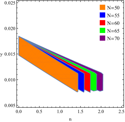
Figure 1: Prediction regions in $\gamma-n$ plane. The left panel is plotted for $\delta=10^{-4}$, while the right one is for $\delta=0.094$.

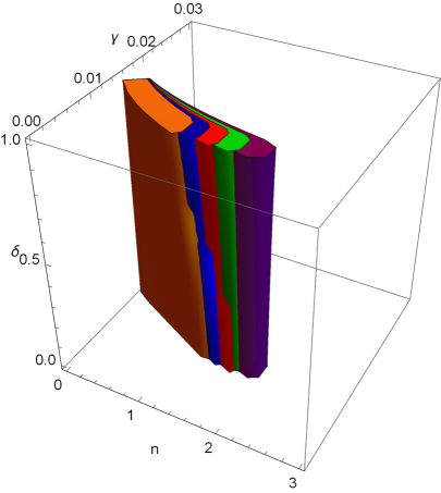
Figure 2: Prediction regions in $(\delta,\gamma,n)$ parameter space.

To match our results with the observations, we consider $0.004<\gamma<0.018$ and $\delta$ takes a small value according to the result of observation Asghari2022 ; Jusufi2022 ; Barrow2021 ; Anagnostopoulos2020 . With the fixed values of $n$ and $\delta$, we depict the predictions of the chaotic potential  (18) in $r_{0.002}-n_{s}$ plane in Fig. (3) in which we overlap our analytical results with Planck 2018 data. These figures show that the value of $r$ decreases as $N$ varies from $50$ to $70$, and an increasing $\gamma$ leads to a smaller value of $n_{s}$. It is obvious that the constant-roll parameter $\gamma$ has an apparent influence on $(r_{0.002},n_{s})$ behavior. With this comparison with the observation, the results show a good consistency for a specific range of the constant-roll parameter $\gamma$ with Planck 2018 data, and the results prefer to the case $\delta=10^{-4}$, $\gamma=0.012$ and $n=1$. It is interesting to note that $n=1$ is also obtained in Tsallis holographic dark energy Keskin2023 . It is easy to see that an increased value of $n$ will lead to mismatching with the observation.

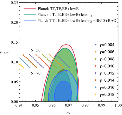
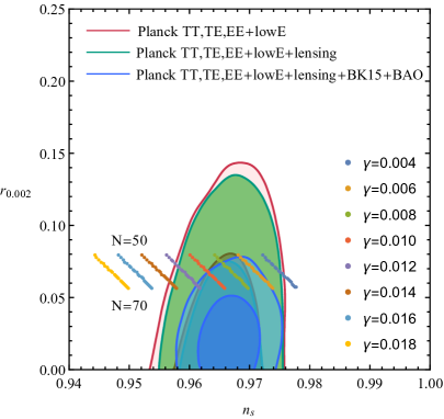
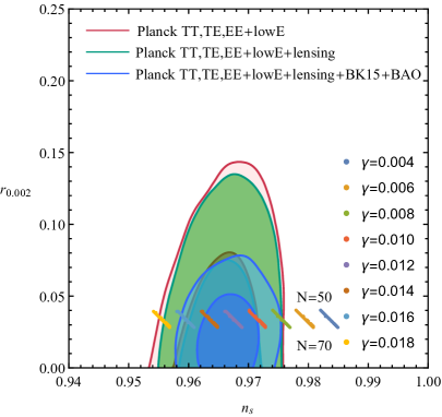
Figure 3: Predictions of the chaotic potential  (18) in $r_{0.002}-n_{s}$ plane. These figures are depicted for: (i) $n=3,\delta=10^{-4}$; (ii) $n=2,\delta=10^{-4}$; (iii) $n=1,\delta=10^{-4}$; (iv) $n=1,\delta=0.094$.

IV Primordial black holes

In previous section, we have analyzed the constant-roll inflation in BHDE model. And then, in this section, we will analyze the evolution of PBHs, which were supposed to formed in the radiation dominated era, in BHDE model. The black holes (BHs) can evolve with an increasing mass by absorbing other matter, stars and BHs. During this process, BHs can emit particles. And the quantum properties of BHs show that the possibility of emitting particles with a thermal spectrum is related to BHs surface gravity Hawking1974 . During the process of emitting particles, BHs may lose mass. In the following, we will analyze the thermal properties of evaporating PBHs. The corresponding PBHs temperatures given as Hawking1974 ; Coogan2021

$$T_{BH}=\frac{\hbar c^{3}}{8\pi GM_{BH}k}\sim 1.06\Big{(}\frac{10^{10}}{M_{BH}}\Big{)}GeV,$$ (25)

where $M_{BH}$ is the total mass of PBHs with the form $M_{BH}=M_{eva}+M_{accr}$, in which $M_{eva}$ and $M_{accr}$ represent the evaporation mass and the accretion mass respectively.

To discuss the evaporation mass of PBHs, we consider the main process to decrease the mass of PBHs is Hawking evaporation which is defined as Page1976a ; Nayak2011

$$\Big{(}\frac{dM}{dt}\Big{)}_{eva}=-\frac{\hbar c^{4}}{G^{2}}\frac{\alpha_{s}}{M^{2}},$$ (26)

where $\alpha_{s}$ is the spin parameter of the emitting particle. Integrating Eq. (26), the evaporation mass of PBHs is obtained

$$M_{eva}=M_{i}\Big{(}1-\frac{t}{t_{eva}}\Big{)}^{\frac{1}{3}},$$ (27)

with

$$t_{eva}=\frac{G^{2}}{\hbar c^{4}}\frac{M^{3}_{i}}{3\alpha_{s}},$$ (28)

where $M_{i}$ is the initial mass of PBHs and $t_{eva}$ denotes the Hawking evaporation time scale. The initial mass of PBHs is given as the order of the particle horizon mass when it was formed Jamil2011

$$M_{i}\approx\frac{c^{3}t_{f}}{G}\approx\frac{10^{12}t_{f}}{10^{-23}}.$$ (29)

Here, $t_{f}$ is the time of its formation. So, the PBHs formed in the late time of the universe must have more mass than that formed in the early time. For the case of PHBs formed at Planck time $10^{-43}s$, it had the mass $10^{-8}kg$. For $t_{f}=2\times 10^{-5}s$, one has $M_{i}=2\times 10^{30}kg$ which is the mass of sun $M_{\odot}$.

Eq. (27) shows the evolution of the evaporation mass of PBHs with respect to $t/t_{eva}$. The evaporation mass decreasing as $t$ approaches to $t_{eva}$ and becomes $0$ for $t=t_{eva}$, which indicates PBHs evaporate completely. The evolution of $M_{eva}/M_{i}$ as the functions of $t/t_{eva}$ is plotted in the left panel of Fig. (4), which is also given in Ref. Bourakadi2023 . So, the Hawking evaporation time scale $t_{eva}$ determines the evaporation time of PBHs. According to Eq. (28), we can find that $t_{eva}$ increases with the increase of $M_{i}$ and decreases with the increase of $\alpha_{s}$. In the right panel of Fig. (4), by considering the evaporation time $t_{eva}$ as a function of the initial mass of PBHs $M_{i}$, we have plotted the relation between $t_{eva}$ and $M_{i}$. The red dashed line in this figure represents the current age of the universe. This figure shows that the PBHs need more time to achieve a complete evaporation with the increase of the initial mass, and it needs a evaporation time longer than the age of the universe when the initial mass is larger than $5\times 10^{11}kg$, which is shown in Ref. Page1976 . For $\alpha_{s}\sim 10^{-4}$ Page1976a ; Jamil2011 , we can write $t_{eva}$ as

$$t_{eva}\sim 10^{-17}M^{3}_{i}.$$ (30)

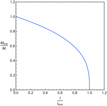
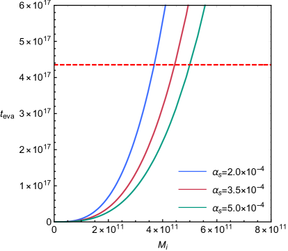
Figure 4: In the left panel, plotted is the evolution of $M_{eva}/M_{i}$ as the function of $t/t_{eva}$. In the right panel, shown is relation between the initial mass of PBHs $M_{i}$ and the evaporation time $t_{eva}$. The red dashed line denotes the age of the universe.

During the process of evaporation, the accretion of fluid surrounding PBHs will prolong the evaporation of PBHs. So, we require to consider the process of the mass accretion rate for PBHs with fluid, which is given as Babichev2004 ; Jamil2011

$$\Big{(}\frac{dM}{dt}\Big{)}_{accr}=\frac{16\pi G^{2}}{c^{3}}M^{2}(\rho_{eff}+p_{eff}).$$ (31)

Here, $\rho_{eff}$ and $p_{eff}$ represent the effective energy density and pressure, respectively. Using Eqs. (3) and  (8), we can obtain

$$\rho_{eff}=\frac{3}{8\pi G}H^{2},\qquad\omega_{eff}=\frac{p_{eff}}{\rho_{eff}}=\frac{2\omega_{\phi}+\delta}{2-\delta},$$ (32)

in which $\omega_{\phi}=p_{\phi}/\rho_{\phi}$. When $\delta$ takes a small value, one can obtain $\omega_{eff}\approx\omega_{\phi}$. Considering $a\sim t^{\frac{2}{3(1+\omega_{eff})}}$ and $H=\frac{2}{3(1+\omega_{eff}t)}$, we can write $\rho_{eff}+p_{eff}$ as

$$\rho_{eff}+p_{eff}=\frac{1}{6\pi G(1+\omega_{eff})t^{2}}.$$ (33)

Here, we consider that $\rho_{eff}+p_{eff}$ evolves with $t$ instead of a constant in Ref. Bourakadi2023 . Then, Eq. (31) can be integrated as

$$M_{accr}=\frac{M_{i}}{1-\beta\Big{(}1-\frac{t_{i}}{t}\Big{)}}$$ (34)

with

$$\beta=\frac{8G}{3c^{2}(1+\omega_{eff})}\frac{M_{i}}{t_{i}},$$ (35)

in which $t_{i}$ is the time that PBHs begins to accrete, $\beta$ denotes the product of the accretion efficiency and the fraction of the horizon mass Nayak2010 . Assuming PBHs begins to accrete at the time when it formed, we obtain $t_{i}=t_{f}$. Then, using Eq. (29), $\beta$ and $t_{i}/t$ can be written as

$$\beta\approx\frac{0.6588}{1+\omega_{eff}},$$ (36)

which indicates $\beta$ is only determined by $\omega_{eff}$ and decreases with the increase of $\omega_{eff}$, and

$$\frac{t_{i}}{t}=\frac{10^{-35}M_{i}}{t},$$ (37)

which equals to $1$ at the time PBHs begins to accrete and decays very fast. So, according to Eq. (34), we can obtain $M_{accr}\simeq M_{i}$ at the initial time $t_{i}$. The evolution curve of $\beta$ and $t_{i}/t$ are plotted in the left and right panel of Fig. (5) respectively. In the left panel of Fig. (6), we have plotted the evolutionary curves for $M_{accr}/M_{i}$ as the function of $t$. This figure shows that $M_{accr}/M_{i}$ increases with the decrease of $\omega_{eff}$, and it increases rapidly in a short time and then keeps as a constant. The right panel of Fig. (6) shows the relation between $M_{accr}/M_{i}$ and $\omega_{eff}$. From these figures, we can see that $M_{accr}/M_{i}$ increases to approach $10^{2}$ when $\omega_{eff}$ decreases from $1/3$ to $-1/3$.

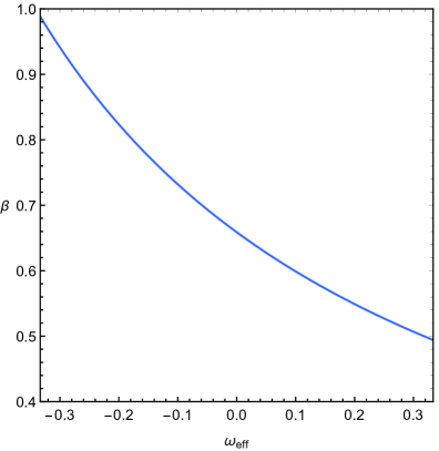
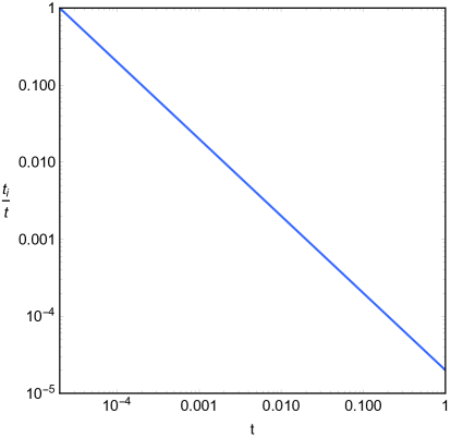
Figure 5: In the left panel, the evolution of $\beta$ as the function of $\omega_{eff}$ is plotted. In the right panel, the evolution of $t_{i}/t$ as the function of $t$ is plotted. The initial mass of PBHs takes the value $M_{i}=M_{\odot}$.

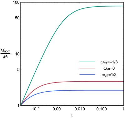
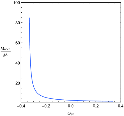
Figure 6: Evolutionary curves of $M_{accr}/M_{i}$. The left panel sets $t$ as the variable, while the right panel sets $\omega_{eff}$. The initial mass of PBHs takes the value $M_{i}=M_{\odot}$.

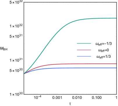
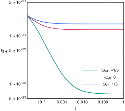
Figure 7: Evolutionary curves of PBH mass $M_{BH}$ and PBH temperature $T_{BH}$. The initial mass of PBHs takes the value $M_{i}=M_{\odot}$.

The left panel of Fig. (7) shows the evolutionary curves of PBHs mass $M_{BH}$ as the function of $t$. From this figure, we can see that $M_{BH}$ increases rapidly in a short time and then keeps as a constant, and $M_{BH}$ increases with the decrease of $\omega_{eff}$. In the right panel of Fig. (7), we have plotted the evolutionary curves of PBHs temperature $T_{BH}$ as the function of $t$. Since $T_{BH}$ is inversely proportional to $M_{BH}$, which is given in Eq. (25), $T_{BH}$ decreases rapidly in a very short time and then becomes a constant, and $T_{BH}$ decreases once $\omega_{eff}$ becomes small. When $\omega_{eff}$ evolves from $1/3$ to $-1/3$, the PBHs temperature $T_{BH}$ decreases from $10^{-21}GeV$ to $10^{-23}GeV$, i.e. $T_{BH}$ decreases from $10^{-8}K$ to $10^{-10}K$.

After inflation ended and PHBs formed, the universe evolves from the radiation dominated epoch to the pressureless matter dominated epoch, and then enters into the dark energy dominated epoch, the effective state of equation parameter evolves from $1/3$ to less than $-1/3$, the accretion mass $M_{accr}$ increases to approach $10^{2}M_{i}$, the PBHs temperature $T_{BH}$ decreases with the increase of $M_{BH}$.

V Conclusion

Based on the holographic principle and the Barrow entropy, a new BHDE model with the apparent horizon as IR cutoff has been proposed and the corresponding Friedmann equation has been modified. In this paper, using the modified Friedmann equation and the constant-roll condition, we calculate the constant-roll parameters $\epsilon_{1}$ and $\epsilon_{2}$, the scalar spectral index parameter $n_{s}$ and the tensor-to-scalar ratio $r$ with the chaotic potential $V_{0}\phi^{n}$. Then, using the Planck 2018 data, we plot the $\gamma-n$ plane, the $(\delta,\gamma,n)$ parameter space and the $r_{0.002}-n_{s}$ plane and then obtain a suitable value of the power exponent $n=1$, the parameter of BHDE $\delta$ and the second constant-roll parameter $\gamma$.

Then, we discuss the evolution of PBHs, which were formed in the radiation dominated era after inflation ended, in BHDE model. By analyzing the evolution of the evaporation mass $M_{eva}$ and the accretion mass $M_{accr}$ of PBHs with the initial mass $M_{i}=M_{\odot}$ when the effective state of equation parameter evolves from $1/3$ to less than $-1/3$, we find the accretion mass $M_{accr}$ increases to approach $10^{2}M_{\odot}$ which is in the mass window of PBHs, the PBHs mass $M_{BH}$ increases to $10^{32}kg$ and the temperature $T_{BH}$ decreases to $10^{-10}K$.

- (1) A. Guth, Phys. Rev. D 23, 347 (1981).
- (2) A. Linde, Phys. Lett. B 108, 389 (1982).
- (3) V. Mukhanov, G. Chibisov, JETP Lett. 33, 532 (1981).
- (4) A. Lewis, A. Challinor, A. Lasenby, Astrophys. J. 538, 473 (2000).
- (5) F. Bernardeau, S. Colombi, E. Gaztanaga, R. Scoccimarro, Phys. Rep. 367, 1 (2002).
- (6) S. Weinberg, Cosmology, Oxford Univ. Press (2008).
- (7) Planck Collaboration, Astron. Astrophys. 641, A10 (2020).
- (8) M. Maggiore, Gravitational Waves, Oxford Univ. Press (2018).
- (9) H. Noh and J. Hwang, Phys. Lett. B 515, 231 (2001).
- (10) J. Martin, H. Motohashi, T. Suyama, Phys. Rev. D 87, 023514 (2013).
- (11) K. Dimopoulos, Ultra slow-roll inflation demystified. Phys. Lett. B 775, 262 (2017).
- (12) C. Pattison, V. Vennin, H. Assadullahi, and D. Wands, JCAP 08, 048 (2018).
- (13) H. Motohashi, A. Starobinsky, J. Yokoyama, JCAP 09, 018 (2015).
- (14) Q. Gao, Sci. China Phys. Mech. Astron. 60, 090411 (2017).
- (15) Q. Gao, Sci. China Phys. Mech. Astron. 61, 70411 (2018).
- (16) Z. Yi, Y. Gong, JCAP 03, 052 (2018).
- (17) L. Anguelova, P. Suranyi, L.C.R. Wijewardhana, JCAP 02, 004 (2018).
- (18) F. Cicciarella, J. Mabillard, M. Pieroni, JCAP 01, 024 (2018).
- (19) M. Guerrero, D. Rubiera-Garcia, D. Gomez, Phys. Rev. D 102, 123528 (2020).
- (20) S. Nojiri, S. Odintsov, and V. Oikonomou, Class. Quantum Grav. 34, 245012 (2017).
- (21) H. Motohashi, A. Starobinsky, Eur. Phys. J. C 77, 538 (2017).
- (22) S. Panda, A. Rana, and R. Thakur, Eur. Phys. J. C 83, 297 (2023).
- (23) K. Bourakadi, M. Koussour, G. Otalora, M. Bennai, and T. Ouali, Physics of the Dark Universe 41, 101246 (2023).
- (24) H. Motohashi and A. Starobinsky, JCAP 11, 025 (2019).
- (25) A. Mohammadi, T. Golanbari, S. Nasri, and K. Saaidi, Phys. Rev. D 101, 123537 (2020).
- (26) S. Lahiri, Mode. Phys. Lett. A 37, 2250003 (2022).
- (27) R. Herrera, M. Shokri, and J. Sadeghi, Physics of the Dark Universe 41, 101232 (2023).
- (28) A. Mohammadi, Physics of the Dark Universe 36, 101055 (2022).
- (29) A. Keskin and K. Kurt, Eur. Phys. J. C 83, 72 (2023).
- (30) S. Hawking, Mon. Not. Roy. Astron. Soc. 152, 75 (1971).
- (31) B. Carr and S. Hawking, Mon. Not. Roy. Astron. Soc. 168, 399 (1974).
- (32) G. Chapline, Nature 253, 251 (1975).
- (33) S. Bird, I. Cholis, J. Munoz, Y. Ali-Haimoud, M. Kamionkowski, E. Kovetz, A.Raccanelli, and A. Riess, Phys. Rev. Lett. 116, 201301 (2016).
- (34) M. Sasaki, T. Suyama, T. Tanaka, and S. Yokoyama, Phys. Rev. Lett. 117, 061101 (2016).
- (35) B. Abbott et al. (LIGO Scientific Collaboration and Virgo Collaboration), Phys. Rev. D 93, 122003 (2016).
- (36) J. Barrow and B. Carr, Phys. Rev. D 54, 3920 (1996).
- (37) J. Bhadra and U. Debnath, Int. J. Theor. Phys. 53, 645 (2013).
- (38) G. Aliferis and V. Zarikas, Phys. Rev. D 103, 023509 (2021).
- (39) A. Chanda and B. Paul, Eur. Phys. J. C 82, 616 (2022).
- (40) K. Bourakadi, B. Asfour, Z. Sakhi, M. Bennai, and T. Ouali, Eur. Phys. J. C 82, 792 (2022).
- (41) B. Carr and J. Lidsey, Phys. Rev. D 48, 543 (1993).
- (42) P. Ivanov, P. Naselsky, and I. Novikov, Phys. Rev. D 50, 7173 (1994).
- (43) J. Yokoyama, Phys. Rev. D 58, 083510 (1998).
- (44) J. Garcia-Bellido and E. Ruiz Morales, Physics of the Dark Universe 18, 47 (2017).
- (45) M. Biagetti, G. Franciolini, A. Kehagias, and A. Riotto, JCAP 07, 032 (2018).
- (46) C. Fu, P. Wu, and H. Yu, Phys. Rev. D 102, 043527 (2020).
- (47) M. Davies, P Carrilho, and D. Mulryne, JCAP 06, 019 (2022).
- (48) H. Di and Y. Gong, JCAP 07, 007 (2018).
- (49) C, Fu, P, Wu, and H, Yu, Phys. Rev. D 100, 063532 (2019).
- (50) G. Ballesteros, J. Rey, M. Taoso, and A. Urbano, JCAP 08, 043 (2020).
- (51) Y. Liu, Q. Wang, B. Su, and N. Li, Physics of the Dark Universe 34, 100905 (2021).
- (52) D. Figueroa, S. Raatikainen, S. Rasanen, and E. Tomberg, JCAP 05, 027 (2022).
- (53) H. Motohashi, S. Mukohyama, and M. Oliosi, JCAP 03, 002 (2020).
- (54) E. Tomberg, Phys. Rev. D 108, 043502 (2023).
- (55) S. Clesse and J. Garcia-Bellido, Phys. Rev. D 92, 023524 (2015).
- (56) M. Kawasaki, A. Kusenko, Y. Tada, and T. T. Yanagida, Phys. Rev. D 94, 083523 (2016).
- (57) B. Carr, F. Kuhnel, and M. Sandstad, Phys. Rev. D 94,083504 (2016).
- (58) K. Inomata, M. Kawasaki, K. Mukaida, Y. Tada, and T. Yanagida, Phys. Rev. D 96, 043504 (2017).
- (59) K. Inomata, M. Kawasaki, K. Mukaida, and T. Yanagida, Phys. Rev. D 97, 043514 (2018).
- (60) B. Carr and J. Silk, Mon. Not. Roy. Astron. Soc. 478, 3756 (2018).
- (61) C. Germani and I. Musco, Phys. Rev. Lett. 122, 141302 (2019).
- (62) A. Kusenko, M. Sasaki, S. Sugiyama, M. Takada, V. Takhistov, and E. Vitagliano, Phys. Rev. Lett. 125, 181304 (2020).
- (63) R. Calabrese, D. Fiorillo, G. Miele, S. Morisi, and A. Palazzo, Phys. Lett. B 829, 137050 (2022).
- (64) J. de Freitas Pacheco, E. Kiritsis, M. Lucca, and J. Silk, Phys. Rev. D 107, 123525 (2023).
- (65) M. Flores and A. Kusenko, JCAP 05, 013 (2023).
- (66) V. Dike, D. Gilman, T. Treu, Mon. Not. Roy. Astron. Soc. 522, 5434 (2023).
- (67) J. de Freitas Pacheco and J. Silk, Phys. Rev. D 101, 083022 (2020).
- (68) G. Fuller, A. Kusenko, and V. Takhistov, Phys. Rev. Lett. 119, 061101 (2017).
- (69) C. Keith, D. Hooper, N. Blinov, and S. McDermott, Phys. Rev. D 102, 103512 (2020).
- (70) M. Kawasaki, A. Kusenko, and T. Yanagida, Phys. Lett. B 711, 1 (2012).
- (71) K. Inomata, M. Kawasaki, K. Mukaida, Y. Tada, and T. Yanagida, Phys. Rev. D 95, 123510 (2017).
- (72) D. Page, Phys. Rev. D 13, 198 (1976).
- (73) F. Kuhnel and K. Freese, Phys. Rev. D 95, 083508 (2017).
- (74) B. Carr, M. Raidal, T. Tenkanen, V. Vaskonen, and H. Veermae, Phys. Rev. D 96, 023514 (2017).
- (75) R. DAgostino, R. Giambo, and O. Luongo, Phys. Rev. D 107, 043032 (2023).
- (76) S. Hsu, Phys. Lett. B 594 13 (2004).
- (77) R. Horvat, Phys. Rev. D 70 087301 (2004).
- (78) M. Li, Phys. Lett. B 603 1 (2004).
- (79) E. Witten, Adv. Theor. Math. Phys. 2 253 (1998).
- (80) R. Bousso, Rev. Modern Phys. 74 825 (2002).
- (81) J. D. Barrow, Phys. Lett. B 808 135643 (2020).
- (82) E. N. Saridakis, Phys. Rev. D 102 123525 (2020).
- (83) F. K. Anagnostopoulos, S. Basilakos, and E. N. Saridakis, Eur. Phys. J. C 80 826 (2020).
- (84) S. Srivastava and U. K. Sharma, Int. J. Geom. Methods Mode. Phys. 18 2150014 (2021).
- (85) A. Sheykhi, Phys. Rev. D 103, 123503 (2021).
- (86) A. Oliveros, M. Sabogal, and M. Acero, Eur. Phys. J. Plus 137, 783 (2022).
- (87) Q. Huang, H. Huang, B. Xu, F. Tu, and J. Chen, Eur. Phys. J. C 81, 686 (2021).
- (88) P. Adhikary, S. Das, S. Basilakos, and E. Saridakis, Phys. Rev. D 104, 123519 (2021).
- (89) A. Mamon, A. Paliathanasis, and S. Saha, Eur. Phys. J. Plus 136, 134 (2021).
- (90) S. Rani and N. Azhar, Universe 7, 268 (2021).
- (91) G. Luciano, Phys. Rev. D 106, 083530 (2022).
- (92) S. Nojiri, S. Odintsov, and T. Paul, Phys. Lett. B 825, 136844 (2022).
- (93) B. Paul, B. Roy, and A. Saha, Eur. Phys. J. C 82, 76 (2022).
- (94) G. Luciano, Physics of the Dark Universe 41, 101237 (2023).
- (95) N. Boulkaboul, Physics of the Dark Universe 40, 101205 (2023).
- (96) R. Pankaj, U. Sharma, and N. Ali, Astrophys Space Sci. 368, 15 (2023).
- (97) S. Ghaffari, G. Luciano, and S. Capozziello, Eur. Phys. J. Plus 138, 82 (2023).
- (98) M. Asghari and A. Sheykhi, Eur. Phys. J. C 82, 388 (2022).
- (99) K. Jusufi, M. Azreg-Ainou, M. Jamil, and E. Saridakis, Universe 8, 102 (2022).
- (100) J. Barrow, S. Basilakos, and E. Saridakis, Phys. Lett. B 815, 136134 (2021).
- (101) F. Anagnostopoulos, S. Basilakos, and E. Saridakis, Eur. Phys. J. C 80, 826 (2020).
- (102) J. Barrow, Phys. Lett. B 808, 135643 (2020).
- (103) S. Nojiri, S. Odintsov, and V. Oikonomou, Phys. Rep. 692, 1 (2017).
- (104) J. Hwang and H. Noh, Phys. Rev. D 71, 063536 (2005).
- (105) Planck Collaboration, AA 641, A10 (2020).
- (106) S. Hawking, Nature 248, 30 (1974).
- (107) A. Coogan, L. Morrison, and S. Profumo, Phys. Rev. Lett. 126, 171101 (2021).
- (108) D. Page, Phys. Rev. D 13, 198 (1976).
- (109) B. Nayak and L. Singh, Pramana 76, 173 (2011).
- (110) M. Jamil and A. Qadir, Gen. Relativ. Gravit. 43, 1069 (2011).
- (111) E. Babichev, V. Dokuchaev, and Y. Eroshenko, Phys. Rev. Lett. 93, 021102 (2004).
- (112) B. Nayak and L. Singh, Phys. Rev. D 82, 127301 (2010).