Continuous Treatment Effect Estimation
Using Gradient Interpolation and Kernel Smoothing

Abstract

We address the Individualized continuous treatment effect (ICTE) estimation problem where we predict the effect of any continuous-valued treatment on an individual using observational data. The main challenge in this estimation task is the potential confounding of treatment assignment with an individual’s covariates in the training data, whereas during inference ICTE requires prediction on independently sampled treatments. In contrast to prior work that relied on regularizers or unstable GAN training, we advocate the direct approach of augmenting training individuals with independently sampled treatments and inferred counterfactual outcomes. We infer counterfactual outcomes using a two-pronged strategy: a Gradient Interpolation for close-to-observed treatments, and a Gaussian Process based Kernel Smoothing which allows us to downweigh high variance inferences. We evaluate our method on five benchmarks and show that our method outperforms six state-of-the-art methods on the counterfactual estimation error. We analyze the superior performance of our method by showing that (1) our inferred counterfactual responses are more accurate, and (2) adding them to the training data reduces the distributional distance between the confounded training distribution and test distribution where treatment is independent of covariates. Our proposed method is model-agnostic and we show that it improves ICTE accuracy of several existing models. We release the code at: https://github.com/nlokeshiisc/GIKS˙release.

1 Introduction

Many applications require the estimation of the effect of a continuous treatment variable on an individual’s response. For example, in healthcare we need to estimate the effect of the dose of a drug on the recovery of a patient, in economics, we need to estimate the effect of a discount on the sales of a product, and in public policy, we need to estimate the effect of income on a person’s longevity. In all these cases, observational data is available in abundance but controlled experiments to estimate these effects exactly either raise ethical issues or incur hidden costs. The main challenge in estimating treatment effects from observational data is that in the observed data each individual is associated with one treatment dose which may be correlated with observed covariates of the individual, but during deployment, we need to estimate outcomes on all treatment doses, thereby making dose independent of the individual in the test data distribution.

Several prior work have proposed to correct the above mismatch but most of these have focused on binary treatments. Broadly, most methods rely on a combination of these three strategies: (1) Learn shared representation of the feature with treatment specific outcome prediction (Shalit, Johansson, and Sontag 2017), (2) Impose regularizers to make feature representations distributionally independent of the treatment (Shalit, Johansson, and Sontag 2017), (3) Exploit the overlap assumption to impose instance-specific counterfactual losses in the learned feature space (Alaa and Van Der Schaar 2017; Zhang, Bellot, and Schaar 2020). Recently, a subset of these strategies have been extended to the case of continuous treatments where some have focused on extending the neural architecture to handle continuous treatments (Schwab et al. 2020; Nie et al. 2021; Zhang et al. 2022), and others extend the distributional regularizers (Nie et al. 2021; Bellot, Dhir, and Prando 2022). However, as we show in our experiment evaluation, such regularizers are not too effective in reducing individual continuous treatment effect estimation errors.

In this paper, we propose to directly minimize counterfactual loss for each individual by inferring outcomes at independently sampled new treatments. We infer outcomes using two types of smoothing strategies. First, by exploiting the differentiability of the response function to treatment, we infer the counterfactual response by gradient interpolation (Nasery et al. 2021). Second, by exploiting the property of overlap required for the identifiability of ICTE from observational data, we infer a counterfactual response by using a Gaussian process over feature kernels. We handle the potential unreliability of the inferred outcomes by down-weighing examples based on the variance of the GP estimate. We show that individual-level counterfactual losses are significantly more effective in learning ICTE compared to distributional regularizers, particularly in a mini-batch setting. We attribute the reasons for the observed gains of our method to two factors: (1) the inferred outcomes from the data are more accurate than a baseline that is just trained on an observational dataset, and (2) the augmented data makes the training distribution closer to the test distribution.

We make the following contributions in this paper:

• We address the ICTE problem by directly minimizing loss on inferred counterfactual outcomes of new treatments applied to training instances. We infer counterfactual outcomes by (1) gradient interpolation justified by the differentiability of the response function to treatments, and (2) kernel smoothing based on the overlap assumption of covariates and treatment.

• We evaluate our method on five benchmark data and show that we consistently outperform six existing state-of-the-art methods on ICTE. We also demonstrate the application of our model in two medical settings.

• We explain the reasons for the observed gains by showing that our proximity-inferred outcomes are more accurate than the factual model, and the augmentation reduces the confounding between treatment and covariates.

• We show that our method is model-agnostic and provides gains on several existing model architectures.

2 Problem Formulation

We use random variables: $X\in\mathcal{X}\subset\mathbb{R}^{d_{x}}$ for the individual’s covariates, $T\in\mathcal{T}\subset\mathbb{R}$ for treatments, and $Y(t)\in\mathbb{R}$ for potential outcomes or response when an individual is given treatment $t$. Our objective is to estimate the individual treatment effect $\mathbb{E}[Y(t)|\mathbf{x}]$, which represents the expected outcome when an individual $\mathbf{x}\in\mathcal{X}$ receives treatment $t$. In prior work, this term has also been referred to as the Average Dose-Response Function (ADRF), denoted as $\mu(\mathbf{x},t)$. We adopt the Neyman–Rubin causal model (Pearl and Press 2000) and estimate ADRF using the Potential Outcomes Framework. The primary challenge is to learn $\mu(\mathbf{x},t)$ from an observational dataset where each $\mathbf{x}$ is exposed to only one treatment dose, whose selection depends on $\mathbf{x}$ making the covariates correlated with the treatment.

The observational dataset $D$ comprises $N$ samples $\{(\mathbf{x}_{i},t_{i},y_{i})\}_{i=1}^{N}$. Each $\mathbf{x}_{i}\in\mathcal{X}\subset\mathbb{R}^{d_{x}}$ denotes the covariate observed before an individual is exposed to a treatment; $t_{i}\in\mathcal{T}\subset\mathbb{R}$ is the value of continuous treatment $T$ applied on the $i$-th instance and $y_{i}\in\mathbb{R}$ captures the outcome observed for $\mathbf{x}_{i}$ under the treatment dose $t_{i}$. We use $t^{\text{CF}}_{i}\neq t_{i}$ to denote any new treatment that is not observed in $D$.

Following prior work, to ensure the identifiability of ICTE from the observational dataset, we make the following assumptions:

1. Overlap of treatment: which states that every individual has a non-zero probability of being assigned any treatment i.e., $\Pr(t|\mathbf{x})\in(0,1)\;\forall\mathbf{x}\in\mathcal{X},t\in\mathcal{T}$

2. identifiability of causal effect: which states that the observed covariates $\mathcal{X}$ block all the backdoor paths between the treatments ${\mathcal{T}}$ and outcomes $Y$.

3. Differentiability of ADRF: We assume that ADRF $\mu(\mathbf{x},t)$ is differentiable w.r.t. treatment $t$.

Assumptions A1, and A2 are standard assumptions needed for causal inference and under them, we can claim that $\mathbb{E}[Y(t)|X]=\mathbb{E}[Y|t,X]$.

Following prior work  (Nie et al. 2021; Shalit, Johansson, and Sontag 2017; Schwab et al. 2020), we model the ADRF $\mu$ using a composition of two neural networks as $\mu(\mathbf{x},t)=\eta(\Phi(x),t)$, where $\Phi:\mathbb{R}^{d_{x}}\rightarrow\mathbb{R}^{d_{e}}$ embeds the covariates $\mathbf{x}$, and $\eta:\mathbb{R}^{d_{e}}\times\mathbb{R}\rightarrow\mathbb{R}$ predicts the average response given the embedding of an individual $\Phi(\mathbf{x})$, at a treatment dose $t$. Many recent models e.g. DRNet (Schwab et al. 2020), VCNet (Nie et al. 2021) follow this framework. Our default choice is to model the embedding network $\Phi$ using a simple feed-forward neural network and to make the $\eta$ network sensitive to $t$ using VCNet (Nie et al. 2021), a state-of-the-art network for continuous treatment effect inference. The parameters $\theta\in\mathbb{R}^{d_{\theta}}$ of the $\eta$ network are obtained as predictions from another network $G_{\psi}:\mathbb{R}\rightarrow\mathbb{R}^{d_{\theta}}$. The $G_{\psi}$ network uses spline bases to ensure a smooth variation of $\theta$ with $t$. Thus, we can express $\eta\big{(}\Phi(\mathbf{x}),t\big{)}=\eta\big{(}\Phi(\mathbf{x});\theta=G_{\psi}(t)\big{)}$, and the only trainable parameters of $\eta$ are the parameters of $G_{\psi}$ i.e. the $\psi$.

The main challenge in learning the parameters of $\mu$ using observational data through standard likelihood training is the discrepancy between the training and test data distributions. The observational dataset $D$ could confound treatment with $\mathbf{x}$, leading to dependence between the observed treatments and $\mathbf{x}$. Specifically, the training instances are drawn from $P(X,T)=P(T|X)P(X)$, where $T\not\perp\!\!\!\perp X$. On the other hand, during inference, we aim to estimate ADRF for an individual under arbitrarily assigned treatments, implying that $T\perp\!\!\!\perp X$. This corresponds to the test instances being drawn from $P^{\text{CF}}(X,T)=P(X)P(T)$. In the following, we show how we address this issue of disparity.

3 GIKS: Our Proposed Approach

Our main idea is to bridge the gap between the train and test distributions with inferred counterfactuals from auxiliary layers that harness data proximity. We start with a base model with $\Phi$ and $\eta$ trained with factual loss on the training data: $\min_{\Phi,\eta}\sum_{i=1}^{N}\ell\big{(}\eta(\Phi(\mathbf{x}_{i}),t_{i}),y_{i}\big{)}$. Note that our losses are model agnostic, they can be integrated on top of several base architectures (c.f. Section 5.2). Thereafter, for each instance $(\mathbf{x}_{i},t_{i},y_{i})$ in the training set, we sample new treatments $t^{\text{CF}}_{i}$ from $P(T)$ and since there is no supervision for $y_{i}(t^{\text{CF}}_{i})$, we infer pseudo-targets $\widehat{y}_{i}(t^{\text{CF}}_{i})$ by leveraging the proximity in the $\Phi(X)$ and $T$ space to other training examples in two ways: First, we use the ADRF differentiability assumption (A4) to predict responses for new treatments that are within a small distance $\delta$ of the observed treatment using Taylor’s expansion of $\eta$, and impose a loss, which we call the GI loss $\mathcal{L}_{\text{GI}}$. Second, for treatments with a larger distance $|t^{\text{CF}}_{i}-t_{i}|>\delta$, we rely on the overlap assumption (A1) and employ kernel smoothing in the embedding space $\Phi(\mathbf{x})$ over samples $\mathbf{x}_{j}$ in $D$, whose observed treatments are close to $t^{\text{CF}}_{i}$. This gives us an inferred $\widehat{y}_{i}(t^{\text{CF}}_{i})$ and variance $\widehat{\sigma}^{2}(\widehat{y}(t^{\text{CF}}_{i}))$. We use these to impose a confidence-weighted loss which we call $\mathcal{L}_{\text{KS}}$. We elaborate on these two losses:

3.1 Gradient Interpolated Inferred Counterfactual Outcomes

Since, we assume that the learned ADRF $\mu(\mathbf{x}_{i},t_{i})=\eta(\Phi(\mathbf{x}_{i}),t_{i})$ is differentiable w.r.t. $t$, for any new $t^{\text{CF}}_{i}$ that lies close to $t_{i}$, we can infer its response using a first-order Taylor series expansion of $\mu$ around $t^{\text{CF}}_{i}$, and use these to impose instance-specific counterfactual loss as follows:

$$\min_{\Phi,\eta}\mathcal{L}_{\text{GI}}=\sum_{i=1}^{N}\mathcal{L}(\eta(\Phi(\mathbf{x}_{i}),t^{\text{CF}}_{i}),\widehat{y}_{i}(t^{\text{CF}}_{i}))$$ (1)

$$~{}~{}~{}\text{where}~{}~{}\widehat{y}_{i}(t^{\text{CF}}_{i})=y_{i}-(t_{i}-t^{\text{CF}}_{i})\frac{\partial\eta(\Phi(\mathbf{x}_{i}),t)}{\partial t}$$ (2)

Despite the spline parameterization of the VCNet, we show in Figure 3, and Table 4 that $\eta(\Phi(\mathbf{x}),t)$ is not smooth enough, and the above GI loss helps. Note that the above loss is different from the gradient penalty used in other methods (Alvarez Melis and Jaakkola 2018; Arjovsky et al. 2019), where the gradient norm $\|\frac{\partial\eta}{\partial t}\|$ is used as a regularizer. Earlier work (Nasery et al. 2021) has shown that such GI induced losses are more effective in increasing the smoothness of a deep network on a continuous input, rather than the proposals by Alvarez Melis and Jaakkola (2018) and Arjovsky et al. (2019).

3.2 Kernel Smoothed Inferred Counterfactual Outcomes

To infer counterfactual responses for new treatments that are distant from the observed ones, we leverage the first assumption of Overlap: $P(t^{\text{CF}}|\mathbf{x})>0$ for all $\mathbf{x}$. On finite training data $D$, this implies that we need to rely on neighbors in $D$ from the $\Phi(X)$ and $T$ space to infer counterfactual outcomes. However, two challenges arise: (1) combining proximity in both the high-dimensional $\Phi(X)$ and low-dimensional $T$ space, and (2) unreliability of responses inferred from sparse neighborhoods. We describe next how we handle these challenges via a Gaussian Process based estimator:

Gaussian Process for Estimating Counterfactual Response

Suppose we wish to infer $\widehat{y}_{i}(t^{\text{CF}}_{i})$ for an observation $(\mathbf{x}_{i},y_{i},t_{i})$. One option is to design a joint kernel over $\Phi(X)$ and $T$, for example, the product kernel(Bellot, Dhir, and Prando 2022) or the Neural Tangent Kernel (NTK) (Jacot, Gabriel, and Hongler 2018) derived from the $\Phi$, $\eta$ network. However, we found the following two-stage approach with a few learned parameters to be more effective.

First we account for proximity in $T$ space, by collecting the instances $(\mathbf{x}_{j},t_{j},y_{j})$, whose observed treatments $t_{j}$ are close to $t^{\text{CF}}_{i}$, i.e., $|t^{\text{CF}}_{i}-t_{j}|\leq\epsilon_{\text{GP}}$, and define a nearest neighbor dataset $D_{\text{NN}}(t^{\text{CF}}_{i})$:

$$D_{\text{NN}}(t^{\text{CF}}_{i})=\{(\mathbf{x}_{j},t_{j},y_{j})\in D|\;\;|t^{\text{CF}}_{i}-t_{j}|\leq\epsilon_{\text{GP}}\},$$ (3)

$$\bm{X}_{\text{NN}},\bm{y}_{\text{NN}}=[\mathbf{x}_{j}\in D_{\text{NN}}(t^{\text{CF}}_{i})],[y_{j}\in D_{\text{NN}}(t^{\text{CF}}_{i})].$$ (4)

Then, to account for proximity in $\Phi$ space, we fit a Gaussian Process (GP) using $D_{\text{NN}}(t^{\text{CF}}_{i})$ as an inducing set (Titsias 2009) to infer counterfactual responses. Specifically, we model $y_{i}(t^{\text{CF}}_{i})$ as:

$$y_{i}(t^{\text{CF}}_{i})=f(\Phi(\mathbf{x}_{i}))+\epsilon,\text{ where }\epsilon\sim\mathcal{N}(0,\sigma^{2})\quad\text{ with, }$$

$$f(\Phi(\mathbf{x}_{i}))\sim GP(0,K(\Phi(\mathbf{x}_{i}),\Phi(\mathbf{x}_{i}^{\prime})))$$

Then we estimate $\widehat{y}_{i}(t^{\text{CF}}_{i})$, the mean of the posterior as:

$$\widehat{y}_{i}(t^{\text{CF}}_{i}) =K(\Phi(\mathbf{x}_{i}),\Phi(\bm{X}_{\text{NN}}))V_{\text{NN}}^{-1}\bm{y}_{\text{NN}}.$$ (5)

where $V_{\text{NN}}=[\sigma^{2}\mathbb{I}+K(\Phi(\bm{X}_{\text{NN}}),\Phi(\bm{X}_{\text{NN}}))]$. Further variance of the estimate $\widehat{\sigma}^{2}[y_{i}(t^{\text{CF}}_{i})]$ is given by:

$$K(\Phi(\mathbf{x}_{i}),\Phi(\mathbf{x}_{i}))$$

$$-K(\Phi(\mathbf{x}_{i}),\Phi(\bm{X}_{\text{NN}}))V_{\text{NN}}^{-1}K(\Phi(\mathbf{x}_{i}),\Phi(\bm{X}_{\text{NN}})).$$ (6)

We leverage the GP variance to down-weigh unreliable outcomes and mitigate their impact on learned parameters. In particular, a large variance indicates a lack of nearby neighbors in $D_{\text{NN}}(t^{\text{CF}}_{i})$ for instance $\mathbf{x}_{i}$. Thus, in a mini-batch setting, we first sample $t^{\text{CF}}_{i}\sim P(T)$ for each individual in the batch, and then obtain mean and variance estimates using the GP for instances where $|t^{\text{CF}}_{i}-t_{i}|>\delta$. We assign a weight $w_{i}(t^{\text{CF}}_{i})\propto\exp(-\widehat{\sigma}^{2}[y_{i}(t^{\text{CF}}_{i})])$ and we apply a weighted loss to minimize the influence of unreliable counterfactuals on the overall loss.

$$\mathcal{L}_{\text{KS}}=\sum_{\begin{subarray}{c}i:\\ |t^{\text{CF}}_{i}-t_{i}|>\delta\end{subarray}}\dfrac{e^{-\widehat{\sigma}^{2}[y_{i}(t^{\text{CF}}_{i})]}}{\displaystyle\sum_{j}e^{-\widehat{\sigma}^{2}[y_{j}(t^{\text{CF}}_{j})]}}\ell(\eta(\Phi(\mathbf{x}_{i}),t^{\text{CF}}_{i}),\widehat{y}_{i}(t^{\text{CF}}_{i}))$$ (7)

We compute the GP quantities $\widehat{y}_{i}(t^{\text{CF}}_{i}),\widehat{\sigma}^{2}_{i}$ in Eq. 7 inside stop_gradient. In practice, the GP is effective only when the outcomes inferred from it outperform those of a baseline model trained solely on the observational dataset. We show that the GP indeed produces better outcomes in Section  5.3. Moreover, we also show that the additional loss on sampled new treatments successfully addresses the discrepancy between the training and counterfactual test distributions, even after suppressing the impact of instances with high variance.

3.3 Estimating Parameters

Fixing GI+GP Parameters

The GI and GP layers for inferring the counterfactual outcomes require three parameters $\delta,\sigma$, and $\epsilon_{\text{GP}}$, which we fix based on the validation dataset. The estimation procedure does not involve training and thus is computationally efficient. The $\delta$ decides if we estimate $\widehat{y}$ from the GI or the GP, and we fix it to minimize average L2 loss over the validation set. We infer the GP-based mean and variance estimates on the validation dataset at observed treatments for different $\epsilon_{\text{GP}}$ and $\sigma$ values and compute the KS loss $\mathcal{L}_{\text{KS}}$ on the validation dataset $D_{\text{val}}$ using Eqn 7. In particular, for a sample $(\mathbf{x},t,y)$ in the validation dataset, its loss is computed on the ground truth label $y$ for the observed treatment $t$ as $\frac{\exp(-\widehat{\sigma}^{2}[y(t)])\cdot\ell(y,\widehat{y}(t))}{\sum_{(x^{\prime},t^{\prime},y^{\prime})\in D_{\text{val}}}\exp(-\widehat{\sigma}^{2}[y^{\prime}(t^{\prime})])}$. Finally, we select the parameter values that yield the lowest loss.

Estimation of $\Phi,\eta$

Our final objective function combines the three losses:

$$\min_{\Phi,\eta}(\mathcal{L}_{\text{factual}}+\lambda_{\text{GI}}\mathcal{L}_{\text{GI}}+\lambda_{\text{KS}}\mathcal{L}_{\text{KS}})$$ (8)

where $\lambda_{\text{GI}},\lambda_{\text{KS}}$ are hyper-parameters that weigh the contributions of the individual loss terms. A brief description of the overall training and inference procedure is described in Algorithm 1.

Algorithm 1 GIKS training

0:  Training Data $D=\{(\mathbf{x}_{i},t_{i},y_{i})\}$, Validation Data $D_{\text{val}},P(T),\lambda_{\text{GI}},\lambda_{\text{KS}}$, # of epochs $\mathrm{Epochs}$, starting epoch for GI loss $\mathrm{Epoch}_{\text{GI}}$, and for KS loss $\mathrm{Epoch}_{\text{GP}}$.

1:  $\Phi,\eta\leftarrow$Train$(\text{VCNET},D)$

2:  $\delta,\sigma,\epsilon_{\text{GP}}\leftarrow\textsc{FixGIGPParams}(D,D_{\text{val}},\Phi,\eta)$

3:  for $e\in[\mathrm{Epochs}]$ do

4:     $\mathrm{loss}\leftarrow\textsc{FactualLoss}(D,\Phi,\eta)$

5:     $t^{\text{CF}}_{i}\sim P(T)$ for all $i\in[|D|]$

6:     $S_{\delta}\leftarrow\{(\mathbf{x}_{i},t_{i},y_{i}):|t_{i}-t^{\text{CF}}_{i}|<\delta\}$

7:     $\mathrm{loss}\leftarrow\mathrm{loss}+\textsc{GILoss}(S_{\delta},\{t^{\text{CF}}_{i}\},\delta,\Phi,\eta)$

8:     $\mathrm{loss}\leftarrow\mathrm{loss}+\textsc{KSLoss}(D\backslash S_{\delta},\{t^{\text{CF}}_{i}\},\epsilon_{\text{GP}},\Phi,\eta)$

9:     $\Phi,\eta\leftarrow\textsc{GradDesc}(\mathrm{loss})$

10:  Return $\Phi,\eta$

 

1:  function $\textsc{GILoss}(S_{\delta},\{t^{\text{CF}}_{i}\},\delta,\Phi,\eta)$

2:  for $(\mathbf{x}_{i},t_{i},y_{i})\in S_{\delta}$ do

3:     $\widehat{y}_{i}(t^{\text{CF}}_{i})\leftarrow y_{i}-(t_{i}-t^{\text{CF}}_{i})\frac{\partial\eta(\Phi(\mathbf{x}_{i}),t)}{\partial t}$

4:  $\textbf{Return}\ \sum_{(\mathbf{x}_{i},t_{i},y_{i})\in S_{\delta}}\mathcal{L}(\eta(\Phi(\mathbf{x}_{i}),t^{\text{CF}}_{i}),\widehat{y}_{i}(t^{\text{CF}}_{i}))$

 

1:  function $\textsc{KSLoss}(D^{\prime},\{t^{\text{CF}}_{i}\},\epsilon_{\text{GP}},\Phi,\eta)$

2:  for $(\mathbf{x}_{i},t_{i},y_{i})\in D^{\prime}$ do

3:     $D_{\text{NN}}(t^{\text{CF}}_{i})\leftarrow$NNbr$(D,\mathbf{x}_{i},t_{i},\epsilon_{\text{GP}})$ (Eq. 4)

4:     with stop_gradient:

5:      $\text{m}_{i}\leftarrow\mathbb{E}[y_{i}(t^{\text{CF}}_{i})\,|\,D_{\text{NN}}(t^{\text{CF}}_{i}),\mathbf{x}_{i}]$ (Eq. 5)

6:      $\hat{\sigma}^{2}_{i}\leftarrow\text{Var}[y_{i}(t^{\text{CF}}_{i})\,|\,D_{\text{NN}}(t^{\text{CF}}_{i}),\mathbf{x}_{i}]$ (Eq. 3.2)

7:  Compute $\mathcal{L}_{\text{KS}}$ using Eq. (7)

8:  Return $\mathcal{L}_{\text{KS}}$

 

4 Related Work

In this section, we briefly review the literature on both discrete and continuous treatment effect estimation.

Discrete Treatment Effect Estimation (DTE)

Discrete treatment effect estimation can be categorized into three approaches: (1) Sample re-weighting methods (Robins, Rotnitzky, and Zhao 1994; Funk et al. 2011), which adjust counterfactual estimates using inverse propensity scores but can be unstable without calibrated propensity score models. (2) Feature matching techniques  (Johansson, Shalit, and Sontag 2016; Caliendo and Kopeinig 2008; Rubin 1973; Schwab, Linhardt, and Karlen 2018; Kallus 2020), which infer pseudo targets by aggregating labels of neighboring instances but are sensitive to distance metrics and lack reliability checks. (3) Regularization-based methods (Shalit, Johansson, and Sontag 2017; Shi, Blei, and Veitch 2019), such as those using Integral Probability Metrics like Wasserstein distance and Maximum Mean Discrepancy, including Targeted Regularization. Such regularizers are introduced to improve Average Treatment Effect (ATE) estimation. Other approaches include adversarial training methods (Yoon, Jordon, and Van Der Schaar 2018; Ozery-Flato, Thodoroff, and El-Hay 2018), variational autoencoders (Louizos et al. 2017; Rissanen and Marttinen 2021; Lu et al. 2020), and non-parametric Gaussian Process methods that discard the mean estimates and directly minimize the variance of counterfactual predictions (Alaa and Van Der Schaar 2017; Zhang, Bellot, and Schaar 2020).

Continuous Treatment Effect Estimation

Existing literature on continuous treatment effect estimation has focused on two aspects: (1) designing better neural architectures, and (2) designing better loss functions and regularizers. The problem of CTE estimation was introduced in  (Schwab et al. 2020), that proposed DRNet, that discretizes dosage values and uses separate last layers for each discrete dosage bin while sharing previous layers. VCNet  (Nie et al. 2021), on the other hand, avoids discretization by ensuring the smoothness of counterfactual predictions through a trainable spline function. Additionally, TransTEE  (Zhang et al. 2022) proposed a Transformer-based representation network specifically designed for text datasets.

VCNet (Nie et al. 2021) introduced a targeted regularizer to address the train-test mismatch and improve ATE estimation accuracy. In (Bellot, Dhir, and Prando 2022), VCNet was extended to use the Hilbert Schmidt Independence criterion as a regularizer for generating treatment-independent embeddings. Another way to enforce independence is by discretizing treatment groups and using an IPM regularizer to make the representations of different treatment groups similar  (Wang et al. 2022). TransTEE  (Zhang et al. 2022) further extended targeted regularizers to handle continuous treatments with a proposed probabilistic targeted regularizer. While targeted regularizers ensure consistent ATE estimates with asymptotic guarantees, they do not account for Individual Treatment Effect estimation. Another method that performs data augmentation like ours is SciGAN (Bica, Jordon, and van der Schaar 2020), which employs a generative adversarial network (GAN) to generate outcomes for new treatments. However, we will demonstrate the unstable training nature of this GAN-based approach in our experiments.

	TARNet	DRNet	SciGAN	TransTEE	VCNet+TR	VCNet+HSIC	GIKS
TCGA-0	1.673 (0.00)	1.678 (0.00)	2.744 (0.00)	0.164 (0.25)	0.163 (0.31)	0.164 (0.29)	0.152
TCGA-1	1.417 (0.00)	1.465 (0.00)	0.907 (0.00)	0.146 (0.00)	0.098 (0.03)	0.096 (0.08)	0.080
TCGA-2	3.365 (0.00)	3.396 (0.00)	1.359 (0.01)	0.201 (0.00)	0.152 (0.00)	0.144 (0.02)	0.127
IHDP	2.731 (0.00)	3.068 (0.00)	–	2.266 (0.00)	2.263 (0.00)	1.961 (0.09)	1.891
NEWS	1.126 (0.00)	1.163 (0.00)	–	1.239 (0.00)	1.107 (0.00)	1.104 (0.00)	1.079

Table 1: Comparison of GIKS with baselines. on CF error. The table includes the mean performance and within brackets, the $p$-values obtained from one-sided paired $t$-tests with GIKS as the base. Values less than 0.05 indicate statistically significant gains. ”–” denotes models that did not converge. GIKS outperforms all the baselines across all datasets, and the results are statistically significant for the majority of them.

	TARNet		DRNet		TransTEE
	Baseline	GIKS	Baseline	GIKS	Baseline	GIKS
TCGA-0	1.678 $\pm$ 0.027	1.077 $\pm$ 0.034	1.673 $\pm$ 0.036	1.073 $\pm$ 0.028	0.164 $\pm$ 0.027	0.165 $\pm$ 0.032
TCGA-1	1.465 $\pm$ 0.039	0.555 $\pm$ 0.011	1.417 $\pm$ 0.049	0.556 $\pm$ 0.013	0.146 $\pm$ 0.024	0.132 $\pm$ 0.021
TCGA-2	3.396 $\pm$ 0.059	0.746 $\pm$ 0.045	3.365 $\pm$ 0.079	0.747 $\pm$ 0.041	0.201 $\pm$ 0.011	0.172 $\pm$ 0.179
IHDP	3.068 $\pm$ 0.126	3.037 $\pm$ 0.227	2.731 $\pm$ 0.333	2.532 $\pm$ 0.169	2.266 $\pm$ 0.182	2.023 $\pm$ 0.193
NEWS	1.163 $\pm$ 0.055	1.159 $\pm$ 0.088	1.126 $\pm$ 0.069	1.129 $\pm$ 0.135	1.239 $\pm$ 0.120	1.176 $\pm$ 0.179

Table 2: Performance comparison of GIKS with base model architecture adopted from three other state of the art methods, viz, TARNet, DRNet and TransTEE on the CF error.

5 Experiments

Dataset

Following the prior work (Nie et al. 2021; Zhang et al. 2022; Bica, Jordon, and van der Schaar 2020), we use five datasets, namely IHDP, NEWS, and TCGA(0-2) on three types of treatments. Across all datasets, $t\in[0,1]$. Details are deferred to the Appendix.

Methods

We compare against six recent state-of-the-art baselines, i.e., TARNet (Shalit, Johansson, and Sontag 2017), DRNet (Schwab et al. 2020). SciGAN (Bica, Jordon, and van der Schaar 2020), TransTEE (Zhang et al. 2022) and VCNet+TR (Nie et al. 2021). Details of methods in Appendix.

	TCGA(0-2)	IHDP	NEWS
lrn rate	$10^{-4}$	$10^{-2}$	$10^{-3}$
$\lambda_{\text{GI}}$	$10^{-1}$	$10^{-4}$	$10^{-2}$
$\lambda_{\text{KS}}$	$10^{-2}$	$10^{-1}$	$10^{-4}$

Table 3: The hyperparameters.

Hyper-Parameter Estimation

We allocate $30\%$ samples as validation dataset to tune hyperparameters. Note, we depend only on factual error and do not require counterfactual supervision even in the validation dataset. GIKS has three hyperparameters: learning rate, $\lambda_{\text{GI}}$, $\lambda_{\text{GP}}$ that are optimized via grid search on factual error of the validation dataset. Further, the GP employs a cosine kernel. We use a batch size of 128, the AdamW optimizer, and early stopping based on factual error on the validation dataset. The results of hyperparameter tuning are presented in Table 3.

Evaluation Metric (CF Error)

Following existing literature, we evaluate performance using CF Error, short for counterfactual estimation error, that measures the prediction accuracy for arbitrary treatments applied on test instances, thus making it suitable for the ICTE problem. Given $N$ test instances, we define the CF error as: $\sqrt{\frac{1}{N}\textstyle\sum_{i=1}^{N}\int_{t^{\text{CF}}_{i}=0}^{1}(y_{i}(t^{\text{CF}}_{i})-\widehat{y}_{i}(t^{\text{CF}}_{i}))^{2}P(t^{\text{CF}}_{i})dt^{\text{CF}}_{i}}$. The error integrates over treatments sampled from $P(T)$ applied to the test instances. In practice, since it is difficult to determine the test time treatment distribution $P(T)$, our default is using a uniform distribution, as followed in earlier work (Bica, Jordon, and van der Schaar 2020), and we present ablations on other candidates of $P(T)$.

5.1 Comparison with SOTA Methods

Table 1 compares our method against all state-of-the-art CTE methods (Section 5) based on CF Error. We make the following observations: (1) GIKS consistently outperforms all baselines on CF error across all datasets, highlighting the suitability of our loss function for ICTE estimation. The statistically significant gains in performance, as indicated by the computed $p$-values from a one-sided paired $t$-test with GIKS as the base, further support the superiority of our approach, except for the TCGA-0 dataset where performance is comparable to the next competing baselines. (2) SciGAN, despite incorporating instance-level counterfactual losses like our approach, demonstrates poor performance due to the challenges associated with training the min-max objectives in adversarial training. Our experiments revealed instances where the error significantly increased for specific dataset seeds, resulting in high result variance. The lack of a control mechanism akin to our GP variance to filter unreliable counterfactual supervision prevented model convergence when the counterfactual supervision provided by the generator was flawed. (3) DRNet and TARNet suffer from poor performance due to their discretization of treatments, which leads to their $\eta$ network being less sensitive to changes in $t$. (4) VCNet with two regularizers: Targeted Regularizer and HSIC are both worse than GIKS. Although HSIC is a better regularizer for the ICTE problem, it still operates at a distribution level rather than at an instance level like GIKS.

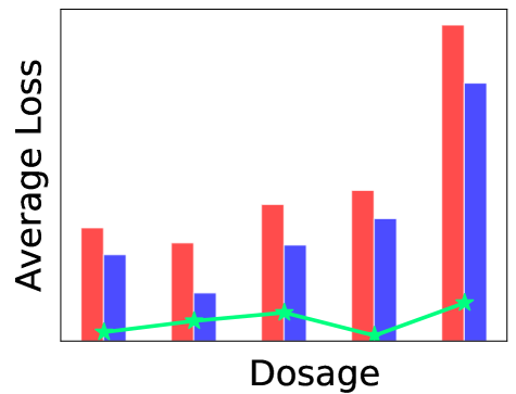
(a)

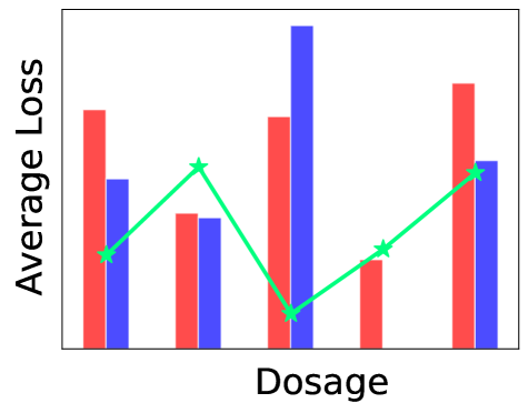
(b)

Figure 1: Losses on Counterfactuals

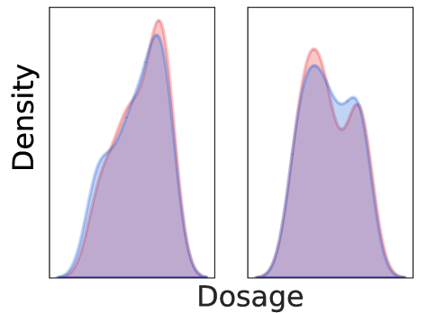
(a)

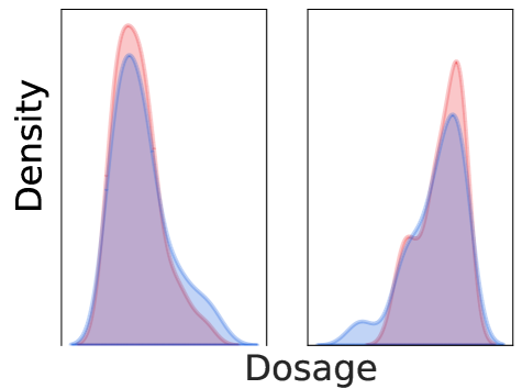
(b)

Figure 2: Training Dosage distribution

5.2 GIKS with Different Base Architectures

The model-agnostic nature of GIKS allows it to be integrated with various base architectures. While VCNet is chosen for its effectiveness with continuous treatments, we explore the potential of GIKS with other networks such as TARNet, DRNet, and TransTEE next. Our experiments, presented in Table 2, show that GIKS enhances the performance of all the base networks.

5.3 Why GIKS Works?

To see why our approach produces better counterfactual estimates, we conduct experiments using the IHDP dataset, and a synthetic dataset taken from  Nie et al. (2021), to answer the following questions:

• Are inferred counterfactuals using neighbors in $\Phi$ and $T$ space more accurate than those obtained from a baseline model that is trained solely on observational dataset $D$?

• For a given individual $\mathbf{x}$, do our augmented loss help reduce the divergence $D(P(\mathbf{x},t)||P(\mathbf{x})P(t))$ between training and test distribution?

We answer the first question by contrasting the performances of two models: (1) a baseline factual model trained solely on the observational dataset $D$ using factual loss $\mathcal{L}_{\text{factual}}$, and (2) our GIKS model trained using algorithm 1. Now, for GIKS to work, we need GP to produce counterfactual estimates that are more accurate than the factual model. To assess this, we compare the losses of the factual model with the losses of GP estimates obtained using Eq. 5 for training instances at randomly sampled new treatments. The results in Figure 1 demonstrate that GP produces more accurate counterfactual estimates than the baseline’s $\eta$ network, except for the middle bin $(0.4,0.6]$ in the synthetic dataset, which has limited instances. The line plot in Figure 1 shows the distribution of examples in each bin. By performing a one-sided paired $t$-test, we confirm that GP’s losses are statistically significantly lower than the factual losses with a $p$-value of 0 for both datasets, providing further confidence in GP’s higher accuracy.

To answer the second question, we compare the treatment distributions used to train the factual model and GIKS for different individuals in the dataset. Figure 2 presents the results for both datasets, showcasing the treatments at which losses were imposed during training for two arbitrarily chosen candidates and their 30 nearest neighbors. We observe that GIKS reduces the skew in the treatment distribution, leading to a lower divergence $D(P(\mathbf{x},t)||P(\mathbf{x})P(t))$. To further validate this observation, we compute the HSIC metric, which resulted in divergence values of 8.30 (0.94) for the factual model of synthetic (IHDP) and 4.9 (0.63) for GIKS of Synthetic (IHDP) dataset. These results, along with the previous findings, provide insights into the effectiveness of GIKS for counterfactual inference.

5.4 Ablation Study

Impact of the Three Losses on GIKS Performance

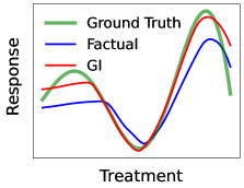
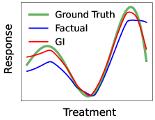
Figure 3: IHDP Individualised Dose-Response Function

Dataset	$\mathcal{L}_{\text{fct}}$	$+\lambda_{\text{GI}}\mathcal{L}_{\text{GI}}$	$\lambda_{\text{KS}}\mathcal{L}_{\text{KS}}$	GIKS
TCGA-0	0.18 (0.10)	0.17 (0.26)	0.17 (0.21)	0.15
TCGA-1	0.09 (0.08)	0.09 (0.62)	0.09 (0.63)	0.09
TCGA-2	0.17 (0.03)	0.17 (0.06)	0.16 (0.01)	0.12
IHDP	2.05 (0.00)	1.91 (0.32)	1.96 (0.10)	1.89
NEWS	1.09 (0.00)	1.08 (0.41)	1.08 (0.23)	1.07

Table 4: CF error for the models trained using different combinations of our loss components.

In this experiment, we analyze the impact of each of the three proposed losses in GIKS by measuring the CF error achieved for models that are trained on different combinations of GIKS losses until convergence. The results are summarized in Table 4. First, observe that neither GI, nor GP is superior over the other, and this lets us conclude that both our loss components have a non-trivial effect on the performance of GIKS. Second, the GI loss alone manages to provide gains over VCNet and complements the smoothness provided by the spline parameterization of the VCNet model. While VCNet focuses on smooth parameter variations of the $\eta$ network with $t$, our $\mathcal{L}_{\text{GI}}$ ensures that the predictions of the $\eta$ network also vary smoothly with $t$. These two methods work together to achieve a smooth ADRF at an instance level. We observe that $\mathcal{L}_{\text{GI}}$ helps in smoothing the predicted Dose-Response Function for treatments close to the observed treatments, as elucidated in Figure 3 for two training instances.

	CF error
NTK	1.925 (0.35)
Dot product	1.882 (0.43)
cosine	1.842

Table 5: GIKS performance using different kernels over $5$ seeds of IHDP dataset.

Kernel Exploration

We study the impact of different types of kernels on the performance of GIKS. We experimented with three kernels: cosine kernel $K(\Phi(\mathbf{x}),\Phi(\mathbf{x}^{\prime}))=\frac{\Phi(\mathbf{x})^{\top}\Phi(\mathbf{x}^{\prime})}{||\Phi(\mathbf{x})||||\Phi(\mathbf{x})||}$, dot product kernel $K(\Phi(\mathbf{x}),\Phi(\mathbf{x}^{\prime}))=\Phi(\mathbf{x})^{\top}\Phi(\mathbf{x}^{\prime})$, and finally NTK kernel $K(\Phi(\mathbf{x}_{i}),\Phi(\mathbf{x}_{j}))={\nabla_{\eta,\Phi}\eta(\Phi(\mathbf{x}_{i}),t_{i})}^{\top}\nabla_{\eta,\Phi}\eta(\Phi(\mathbf{x}_{j}),t_{j})$. Table 5 summarizes the results for the IHDP dataset averaged over $5$ seeds. We present the $p$-values of one-sided paired $t$-test with cosine kernel as the base within bracket. We observe that: (1) Cosine kernel performs better than Dot-product kernel, perhaps because Cosine is invariant to the scale of the embeddings. (2) Even though the NTK kernel defines a joint kernel over $\mathcal{X}$ and ${\mathcal{T}}$ space, unlike GIKS that used a two-stage kernel, computing the NTK Kernel is both computation and memory intensive.

Impact of Alternative $P(T)$

We experimented with alternative distributions for sampling new treatments during training: (1)Marginal treatment distribution, where we sample treatments from the empirical marginal treatment distribution in the observational dataset. (2)Inverse Propensity (IP) distribution, where we discretized the treatments into $10$ bins and trained a propensity model $\pi:\mathcal{X}\rightarrow[10]$ that predicts the treatment bin. Then we sample treatments from a bin chosen with a probability $P(\bullet\,|\,\mathbf{x})=\frac{1}{\pi(\bullet\,|\,\mathbf{x})}$. To make the results comparable, Table 6 presents the CF error tested on uniform distribution across these three training strategies. We also report $p$-values of the one-sided paired $t$-test with default sampling. We observe that GIKS performance is similar across all the sampling strategies, that is possibly because (1) For the IHDP and news dataset, their marginal treatment distribution is close to uniform (3) For IP sampling, the propensity model achieved an accuracy of $100\%$ in predicting the correct bin for both datasets. The inverted propensity scores gave negligible weight to the predicted bin and approximately equal weight to the other bins leading to close to uniform sampling.

	IHDP	NEWS
Marginal	1.902 (0.42)	1.086 (0.09)
IP	1.903 (0.41)	1.080 (0.36)
Uniform	1.891	1.079

Table 6: Sampling strategies for $P(T)$.

	TransTEE	VC+TR	VC+HSIC	GIKS
CF Error	0.42 $\pm$ 0.01	0.43 $\pm$ 0.01	0.43 $\pm$ 0.01	0.42 $\pm$ 0.01
Policy Err.	0.22 $\pm$ 0.03	0.19 $\pm$ 0.02	0.18 $\pm$ 0.00	0.17 $\pm$ 0.01
Rec. Acc.	0.59 $\pm$ 0.02	0.60 $\pm$ 0.02	0.62 $\pm$ 0.04	0.63 $\pm$ 0.01

Table 7: Performance of GIKS vs. baselines on recourse for image setting for skin lesion diagnosis. We report mean $\pm$ std. deviation averaged over $5$ seeds.

5.5 Case Study

We conducted two case studies illustrating the application of treatment effect estimation to Algorithmic Recourse where the goal is to predict the treatment that yields the best outcome. We present the skin lesion diagnosis experiment in this section and defer the insulin prediction experiment to regulate glucose levels to the appendix.

Algorithmic Recourse for Mobile Skin Lesion Diagnosis

We consider an application where users submit skin images to a diagnostic classifier designed for lesion detection. In the event of a user uploading a low-quality image, the classifier might yield an inaccurate diagnosis. Our objective is to guide users in adjusting their image capture settings to enhance diagnostic accuracy. We employed a commonly used skin lesion detection dataset, featuring seven labels, with the classifier predicting a distribution across these seven categories. Our goal in algorithmic recourse is to recommend image settings for which the classifier confidence — probability of the predicted class — is high. As part of the setting (treatment), we consider brightness level of the image. For training the model for counterfactual inference we created an observation dataset $D$, where each instance is a 3-tuple $(t_{i},\phi(\mathbf{x}_{i}),\rho_{i})$. Here, $\mathbf{x}_{i}$ is an initial image, $\phi(\mathbf{x}_{i})$ is its representation, $t_{i}$ denotes the treatment applied to produce post-treatment image $\mathbf{x}^{\prime}_{i}$, and $\rho_{i}$ reflects the classifier’s confidence on the treated image. We introduced selection bias by making the observed treatments depend on $\phi(\mathbf{x}_{i})$. Testing the classifier on a test set with treatments sampled uniformly from $[-0.5,0.5]$, we observed an accuracy of 44%. We evaluate the performance on VCNet architecture of baselines vs. GIKS using Recourse Accuracy which is defined as the accuracy achieved on the test dataset after treating the test images with predicted optimal dosages. We report the recourse performance comparing GIKS with other competing baselines in Table 9. We observed that GIKS achieves the highest recourse accuracy of $63\pm 0.02\%$. We also report dosage policy error which is the difference between the accuracy achievable at the best brightness setting, and the accuracy at the recommended setting by the trained model. Even on this metric, our model performs better.

6 Conclusion

We addressed estimating Individualized Continuous Treatment Effects from observational data, where treatments are confounded with covariates. Our method aims to reduce the mismatch between observed data distribution and the independence needed for counterfactual estimation by sampling new treatments for training instances. We devised two strategies for synthesizing pseudo targets and applying instance-specific counterfactual losses. Experiments on benchmark ICTE datasets showed statistically significant gains over other baselines. We also presented experimental results on two potential medical applications. Future work could include a more thorough investigation of these applications and extending our approach to cases where the overlap assumption is violated as recently highlighted in  (Jesson et al. 2022).

Appendix
(Continuous Treatment Effect Estimation Using Gradient Interpolation and Kernel Smoothing)

Appendix A Sim Glucose Dataset

In this section, we conduct experiments using a real-world glucose simulator to demonstrate the effectiveness of our approach in predicting the impact of insulin on the risk of low and high glucose levels in individuals with Type-1 Diabetes. We used an FDA-approved UVa/Padova Simulator (2008 version) to simulate the dose-response function $\mu$. Our goal is to predict the risks of pumping different dosages of insulin into patients with Type-1 diabetes and thereby design a control algorithm that avoids high risks.

The simulator models risk as a function of the following inputs obtained from a patient: (a) patient covariates, a $13$ dimensional vector that uniquely identifies each patient, (b) the amount of insulin pumped in the patient, (c) the amount of carbs consumed by the patient is her meal. The simulator first predicts the blood glucose levels which are then converted to Magni risk using the formula:

$$\text{risk}(b)=10\cdot(c_{0}\cdot\log(b)^{c_{1}}-c_{2})^{2}$$ (9)

where $b$ denotes the predicted blood glucose levels. Here, $c_{0}$ and $c_{1}$ are constants adjusted to assign lower risks to blood glucose values within the range $[70,180]$ and higher risks otherwise as a safe blood glucose limit is assumed to be in the range of $b\in[70,180]$. Therefore, the objective of any insulin control algorithm is to administer the appropriate insulin doses to maintain blood glucose levels within this safe range. Following prior work (Fox and Wiens 2019), each entry in our observational dataset consists of the covariates $\mathbf{x}$ captured as the measured blood glucose levels 2 hours prior to taking a meal, and the number of carbs consumed during the meal. Now, given a treatment $t$, that denotes the amount of insulin pumped into the blood, our response $y$ captures the maximum risk value over the next two hours of taking the meal.

In our main submission, we did not report results on the TransTEE baseline, which we present here:

	TransTEE	TransTEE (GIKS)	VCNet+TR	VCNet+HSIC	GIKS
CF Error	0.658 (0.223)	0.643 (0.350)	0.628 (0.482)	0.627 (0.500)	0.626
Dosage Policy Error	1.391 (0.628)	1.391 (0.628)	1.856 (0.209)	1.591 (0.427)	1.519

Table 8: Performance of GIKSvs. baselines for insulin treatment on VCNet. We averaged over $5$ seeds.

We observe that for this task, TransTEE architecture performs well on the Dosage policy Error. So, we tested the effectiveness of applying the GIKS losses on the TransTEE architecture and observed that GIKS maintains the performance on the policy error while improving the CF error.

Results on Skin-lesion diagnosis case study. We report the results on the TransTEE baseline for this case study also here:

	TransTEE	VCNet+TR	VCNet+HSIC	GIKS
CF Error	0.42 $\pm$ 0.01	0.43 $\pm$ 0.01	0.43 $\pm$ 0.01	0.42 $\pm$ 0.01
Dosage Policy Error	0.22 $\pm$ 0.03	0.19 $\pm$ 0.02	0.18 $\pm$ 0.00	0.17 $\pm$ 0.01
Recourse Accuracy	0.59 $\pm$ 0.02	0.60 $\pm$ 0.02	0.62 $\pm$ 0.04	0.63 $\pm$ 0.01

Table 9: Performance of GIKSvs. baselines on recourse for image setting for skin lesion diagnosis. We report mean $\pm$ std. deviation averaged over $5$ seeds.

In this experiment, we found that GIKS applied to the VCNet architecture performed the best in all the assessed metrics. We reported std. deviation here as the performance of GIKS was found to be non-overlapping with the baselines.

Appendix B Code / Datasets

We have uploaded the code for GIKS along with the Supplementary material.

Appendix C Limitations

A limitation of our approach is that we make the differentiability (A3) and overlap (A1) assumptions in the dataset without an explicit verification of whether they hold. However, one safe guard we implemented was to depend on the validation dataset for determining the contribution of additional losses arising out of these losses via the GP parameters and the weights assigned to the counterfactual losses ($\lambda_{\text{GI}},\lambda_{\text{KS}}$). In the worst case, we will not provide any gains beyond the baseline factual model. A second limitation is the running time associated with inferring counterfactual responses. While inferring GI based responses is cheap, inferring GP based responses requires a nearest neighbor search over the entire training dataset.

Appendix D Datasets Description

Here we discuss more details on the datasets that we used in our work.

TCGA (0–2) (Bica, Jordon, and van der Schaar 2020)

The TCGA dataset, obtained from The Cancer Genome Atlas project, consists of data on various types of cancer in $9659$ individuals. Each individual is characterized by $4000$ dimensions of gene expression covariates. These covariates are log-normalized and further normalized to have unit variance. The treatment variable represents the dosage of the drug taken by the patient, while the synthetic response models the risk of cancer recurrence. In our experiments, we use three versions of the TCGA dataset proposed in (Bica, Jordon, and van der Schaar 2020), referred to as TCGA(0), TCGA(1), and TCGA(2).

IHDP (Hill 2011)

was originally collected from the Infant Health Development Program and used for binary treatment effect estimation. In the dataset, treatments were assigned through a randomized experiment. It consists of $747$ subjects with $25$ covariates. For the continuous treatment effect (CTE) problem, the dataset was adapted in (Nie et al. 2021) by assigning synthetic treatments and targets.

News (Dua and Graff 2017)

was initially a binary treatment effect dataset but was adapted in (Bica, Jordon, and van der Schaar 2020) for continuous treatments and targets. The treatment variable in this dataset represents the amount of time a user spends reading a news article, while the synthetic response aims to resemble user satisfaction. The dataset consists of $3000$ randomly sampled articles from the New York Times, with $2858$ bag-of-words covariates.

For each of the datasets, we generate several versions of it by using different seeds following prior work. The dataset statistics were provided in Table 1 in the main paper.

Appendix E Synthetic Treatment and Response Generation

We adopt the dataset generation process from the prior methods and we quote the details of dataset generation here for completeness. (Schwab et al. 2020; Nie et al. 2021; Bica, Jordon, and van der Schaar 2020).

IHDP

For treatments in $[0,1]$, we generate responses as in (Nie et al. 2021). Specifically, for a given $\mathbf{x}$, we generate $y$ and $t$ as follows:

$$\tilde{t}\,|\,\mathbf{x} =\frac{2x_{1}}{1+x_{2}}+\frac{2\max(x_{3},x_{5},x_{6})}{0.2+\min(x_{3},x_{5},x_{6})}+2\tanh\left(\frac{5\sum_{i\in S_{\text{dis},2}}(x_{i}-c_{2})}{|S_{\text{dis},2}|}-4+\mathcal{N}(0,0.25)\right),$$ (10)

$$t=(1+\exp(-\tilde{t}))^{-1}$$ (11)

$$y\,|\,\mathbf{x},t =\frac{\sin(3\pi t)}{1.2-t}\cdot\tanh\left(\frac{5\sum_{i\in S_{\text{dis},1}}(x_{i}-c_{1})}{|S_{\text{dis},1}|}\right)+\frac{\exp(0.2(x_{1}-x_{6}))}{0.5+5\min(x_{2},x_{3},x_{5})}\big{)}+\mathcal{N}(0,0.25)$$ (12)

where $S_{\text{con}}=\{1,2,3,5,6\}$ is the index set of continuous covariates, $S_{\text{dis},1}=\{4,7,8,9,10,11,12,13,14,15\}$, $S_{\text{dis},2}=\{16,17,18,19,20,21,22,23,24,25\}$ and $S_{\text{dis},1}\bigcup S_{\text{dis},2}=[25]-S_{\text{con}}$.

Further $c_{1}=\mathbb{E}\left[\frac{\sum_{i\in S_{\text{dis},1}}x_{i}}{|S_{\text{dis},1}|}\right]$, $c_{2}=\mathbb{E}\left[\frac{\sum_{i\in S_{\text{dis},2}}x_{i}}{|S_{\text{dis},2}|}\right]$.

NEWS

First, we generate $v_{1}^{\prime},v_{2}^{\prime},v_{3}^{\prime}$ from $\mathcal{N}(0,1)$, and set $v_{i}=\frac{v_{i}^{\prime}}{\|v_{i}^{\prime}\|}$

$$t\,|\,\mathbf{x} =\text{Beta}\left(2,\left\|\frac{v_{3}^{\top}}{2v_{2}^{\top}\mathbf{x}}\right\|\right),y^{\prime}\,|\,\mathbf{x},t=\exp\left(\frac{v_{2}^{\top}\mathbf{x}}{v_{3}^{\top}\mathbf{x}}-0.3\right)$$ (13)

$$y\,|\,\mathbf{x},t =2(\max(-2,\min(2,y^{\prime}))+20v_{1}^{\top}\mathbf{x})(4(t-0.5)^{2}+\sin\left(\frac{\pi}{2}t\right)+\mathcal{N}(0,0.5)$$ (14)

TCGA(0-2)

First generate $v_{1}^{\prime},v_{2}^{\prime},v_{3}^{\prime}$ from $\mathcal{N}(0,1)$, and set $v_{i}=\frac{v_{i}^{\prime}}{\|v_{i}^{\prime}\|}$ Add noise $\epsilon\sim\mathcal{N}(0,0.2)$. Then, dosage $d\,|\,\mathbf{x},t\sim\text{Beta}(\Phi,t)$, where $\Phi$ (default as 2) is the dosage selection bias. $t_{t}=\frac{\Phi-1}{d^{*}}+2-\Phi$, with $d^{*}$ as optimal dosage for that treatment.

For TCGA (0), we generate $y$ and $d^{*}$ as $y\,|\,\mathbf{x},d=10(v_{1}^{\top}\mathbf{x}+12dv_{3}^{\top}\mathbf{x}-12d^{2}v_{3}^{\top}\mathbf{x}),d^{*}=\frac{v_{2}^{\top}\mathbf{x}}{2v_{3}^{\top}\mathbf{x}}$.

For TCGA(1), we generate $y$ and $d^{*}$ as follows: $y\,|\,\mathbf{x},d=10((v_{1})^{\top}\mathbf{x}+\sin(\pi(\frac{v_{2}^{\top}\mathbf{x}}{v_{3}^{\top}\mathbf{x}}d))),d^{*}=\frac{v_{3}^{\top}\mathbf{x}}{2v_{2}^{\top}\mathbf{x}}$.

For TCGA(2), $y\,|\,\mathbf{x},d=10(v_{1}^{\top}\mathbf{x}+12d(d-0.75\frac{v_{2}^{\top}\mathbf{x}}{v_{3}^{\top}\mathbf{x}})^{2}),d^{*}=0.25\frac{v_{2}^{\top}\mathbf{x}}{v_{3}^{\top}\mathbf{x}}\text{ if }\frac{v_{2}^{\top}\mathbf{x}}{v_{3}^{\top}\mathbf{x}}\geq 1,\text{ else }1$.

Appendix F Additional performance metrics

We present results on four additional metrics that are also reported in the counterfactual inference literature for assessing Average Treatment Effect, finding the dosage that yields the best outcome, etc. We report the mean and one standard deviation from it obtained across different seeds of the datasets.

Factual Error (RMSE)

Here, we report the root mean squared error between the gold factual targets in the test data and the predicted outcomes as

$$\sqrt{\frac{1}{N}\textstyle\sum_{i=1}^{N}(y_{i}(t_{i})-\widehat{y_{i}}(t_{i}))^{2}}.$$ (15)

This metric evaluates the predictive performance of the models on test instances using only their observed dosages.

Table 10: C Comparison of GIKS with baselines TARNet (Shalit, Johansson, and Sontag 2017), DRNet (Schwab et al. 2020), SciGAN (Bica, Jordon, and van der Schaar 2020), TransTEE (Zhang et al. 2022), VCNet+TR (Nie et al. 2021), and VCNet+HSIC (Bellot, Dhir, and Prando 2022) on the Factual error assessed on the test dataset. Factual Error represents the predictive performance specifically on the observed treatments applied to test instances. However, it is not a representative metric for the ICTE problem. ‘–’ indicates non-convergence.

	TARNet	DRNet	SciGAN	TransTEE	VCNet+TR	VCNet+HSIC	GIKS
TCGA-0	1.173 $\pm$ 0.177	1.189 $\pm$ 0.16	3.796 $\pm$ 0.719	0.2 $\pm$ 0.02	0.219 $\pm$ 0.006	0.205 $\pm$ 0.036	0.217 $\pm$ 0.003
TCGA-1	0.887 $\pm$ 0.025	0.92 $\pm$ 0.034	2.384 $\pm$ 0.283	0.199 $\pm$ 0.019	0.215 $\pm$ 0.005	0.205 $\pm$ 0.036	0.219 $\pm$ 0.005
TCGA-2	2.041 $\pm$ 0.047	2.073 $\pm$ 0.07	2.757 $\pm$ 1.352	0.205 $\pm$ 0.024	0.227 $\pm$ 0.004	0.239 $\pm$ 0.006	0.227 $\pm$ 0.005
IHDP	3.398 $\pm$ 0.289	2.978 $\pm$ 0.383	–	2.323 $\pm$ 0.257	2.55 $\pm$ 0.264	2.192 $\pm$ 0.337	2.22 $\pm$ 0.321
NEWS	1.207 $\pm$ 0.049	1.202 $\pm$ 0.042	–	1.356 $\pm$ 0.057	1.327 $\pm$ 0.047	1.14 $\pm$ 0.055	1.197 $\pm$ 0.039

Table 10 shows the results on factual error, where we observe a slight increase on some datasets. This is expected because our counterfactual losses prevent the overfitting of models to just the factual distribution using imposing losses on uniformly sampled counterfactuals with synthesized pseudo-targets. In summary, GIKS trades off some factual accuracy to effectively handle instances that are more likely to occur during the inference stage. TransTEE performs better for factual error because they use powerful transformers to fit the factual distribution.

Dosage Policy Error (DPE)

It is defined as

$$\frac{1}{N}\sum_{i=1}^{N}(y_{i}(t^{*})-y_{i}(\widehat{t}))^{2}$$ (16)

where $t^{*}$ is the ground truth treatment for the best possible outcome, and $\widehat{t}$ is the predicted best treatment. This metric is more relevant in medical datasets than in TCGA. The results are shown in Table 11.

	TARNet	DRNet	TransTEE	VCNet	GIKS
TCGA(0)	0.402 $\pm$ 0.193	0.523 $\pm$ 0.414	0.120 $\pm$ 0.075	0.117 $\pm$ 0.095	0.073 $\pm$ 0.037
TCGA(1)	0.446 $\pm$ 0.028	0.452 $\pm$ 0.023	0.009 $\pm$ 0.007	0.006 $\pm$ 0.001	0.004 $\pm$ 0.005
TCGA(2)	0.793 $\pm$ 0.063	0.819 $\pm$ 0.057	0.007 $\pm$ 0.007	0.005 $\pm$ 0.006	0.004 $\pm$ 0.007

Table 11: This table shows the Dosage Policy Error (DPE) for the TCGA(0-2) datasets. We see that GIKS outperforms the baselines for TCGA(0) and TCGA(2). for TCGA(1), we VCNet gives us the best performance in terms of DPE. These results show that counterfactual losses imposed by GIKS are indeed effective in determining the optimal dosages specific to each individual that can lie beyond the training distribution.

Average Mean Squared Error (AMSE)

This metric is defined as

$$\frac{1}{N}\sum_{i=1}^{N}\int_{0}^{1}(y_{i}(t^{\text{CF}})-\widehat{y_{i}}(t^{\text{CF}}))^{2}P(t^{\text{CF}})dt^{\text{CF}}$$ (17)

It assesses the error in the predicted responses integrated over treatments sampled from training propensity distribution $\pi$, and averaged across all the individuals in test data. The results are shown in the Table 12.

Appendix G AMSE Results

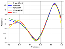
(a)

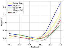
(b)

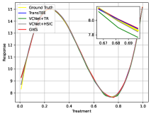
(c)

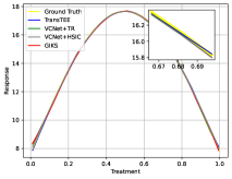
(d)

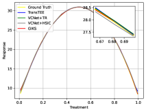
(e)

Figure 4: This Figure shows the ADRF curves for all the baselines and GIKS.

	TARNet	DRNet	TransTEE	VCNet	GIKS
TCGA(0)	5.422 $\pm$ 0.131	5.407 $\pm$ 0.183	0.0294 $\pm$ 0.009	0.039$\pm$0.012	0.028$\pm$0.0174
TCGA(1)	2.778$\pm$0.110	2.637$\pm$0.159	0.0267 $\pm$ 0.009	0.012$\pm$0.003	0.009$\pm$0.001
TCGA(2)	12.586$\pm$0.416	12.364$\pm$0.604	0.0498 $\pm$ 0.007	0.030$\pm$0.007	0.024$\pm$0.006
IHDP	3.477 $\pm$ 1.435	6.660 $\pm$ 0.460	0.951 $\pm$ 0.426	0.883 $\pm$ 0.487	0.519 $\pm$ 0.380
NEWS	0.195 $\pm$ 0.028	0.200 $\pm$ 0.026	0.018 $\pm$ 0.012	0.048 $\pm$ 0.021	0.034 $\pm$ 0.020

Table 12: This table shows the Average Mean Squared Error (AMSE) values meant for Average Treatment Effect assessment for baselines and GIKS. We observe the trend of these results also to be in alignment with the trend for CF Error. Except for NEWS, GIKS outperforms the baselines on all datasets.

We present the AMSE results for all the datasets in the table 12. For TCGA(0-2) we present the DPE in the table 11. We find that on AMSE, our results are consistent with the MISE metric reported in the main paper. On DPE we are the best on two out of three cases.

Appendix H ADRF curves

In the main paper, we showed the Dose Response Function for an individual on IHDP and TCGA(0) datasets. Here we show the average dose Response Function (ADRF) obtained for all the datasets in the Figure 3. For each of these curves, we obtain the ARDF function by averaging the responses of $30$ nearest neighbors in the $\Phi$ space.

For the NEWS dataset, the methods are not able to fit the ADRF curve perfectly because the training instances have an irreducible additive gaussian noise sampled from $\mathcal{N}(0,0.5)$ in their response $y$, as shown in the Eqn 14. This has not been an issue with other datasets since the scale of $y$ for them is much larger compared to $0.5$; while for NEWS, it is comparable. This leads to the irreducible noise in the dataset having a significant impact on the response variable and this makes the ground truth ADRF curve more irregular.

All curves predict the treatment effect very well for TCGA(0-2), hence the curves seem coincident. We provide a zoomed-in section of the graph for a small range of treatments to better illustrate that GIKS achieves a marginally better fit of the ground-truth ADRF compared to the baselines.

Appendix I Theoretical Analysis

The starting point for our theoretical analysis is Theorem 1 from Bellot, Dhir, and Prando (2022) that gives the generalization bound for the counterfactual prediction error. We quote the theorem here:

Theorem 1: (Generalization bound for the average counterfactual error). Assume that the unit expected loss functions $l_{h,\phi}(x,t)/B_{\phi}\in G$ for $B_{\phi}>0$ for all $x\in\mathcal{X}$ and $t\in\mathcal{T}$, where $G$ is a family of functions $g:\mathcal{R}\times\mathcal{T}\rightarrow\mathbb{R}$. Then,

$$\epsilon_{CF}\leq\epsilon_{F}+B_{\phi}\cdot\sup_{g\in G}\left|\int_{\mathcal{T}}\int_{\mathcal{R}}g(\mathbf{r},t)\cdot\left(p_{\phi}(\mathbf{r})p_{\phi}(t)-p_{\phi}(\mathbf{r},t)\right)d\mathbf{r}dt\right|$$ (18)

In this expression, $\epsilon_{CF}$ represents the error observed on samples from the counterfactual test distribution, while $\epsilon_{F}$ corresponds to the error on the training distribution. The key insight derived from this theorem is that the additional error during testing is bounded by the second term, which quantifies the dependence between $X$ and $T$. This term equals zero only when $X$ is independent of $T$. Consequently, reducing the counterfactual error is possible by augmenting samples that meet two criteria: (a) the augmented samples provide reliable supervision for $y$, and (b) the augmented dataset exhibits less dependence between $X$ and $T$ than the given training dataset.

In this section, we explore a simplified scenario where both $X$ and $T$ are real-valued ($X\in\mathbb{R}$ and $T\in\mathbb{R}$). The joint distribution between $X,T$ during test is $\mathcal{N}(0,\sigma^{2}I)$ where $I$ is the $2\times 2$ identity matrix, where as during training $X,T$ are correlated $\mathcal{N}(0,\begin{pmatrix}\sigma^{2}&\rho\\ \rho&\sigma^{2}\end{pmatrix})$ where $\rho$ controls the covariance between $X,T$. We assume that the potential outcome $\mu(x,t)$ is $\tau^{\prime}$-smooth in $\mathbf{x}$ and $\delta^{\prime}$-smooth in $t$. Additionally, for an observed sample $(x_{i},t_{i},y_{i})$, we aim to synthesize a pseudo-outcome $\hat{y}(x_{i},t^{\text{CF}}_{i})$ for a new treatment $t^{\text{CF}}_{i}\neq t_{i}$. Let us define the data augmentation with GIKS as successful if the error introduced in the pseudo-outcome is bounded by $\tau$, expressed as $|\hat{y}(x_{i},t^{\text{CF}}_{i})-\mu(x_{i},t^{\text{CF}}_{i})|\leq\tau$. We analyze the specific conditions under which GIKS can achieve this objective.

Because $\mu(x,t)$ is $\tau^{\prime}$ smooth in $x$, we have:

$$\frac{|\mu(x,t)-\mu(x^{\prime},t)|}{|x-x^{\prime}|}<\tau^{\prime}\implies|\mu(x,t)-\mu(x^{\prime},t)|<\tau^{\prime}|x-x^{\prime}|$$ (19)

By setting $\tau^{\prime}|x-x^{\prime}|<\tau$, we establish the condition $|x-x^{\prime}|<\frac{\tau}{\tau^{\prime}}$. This condition indicates that if GIKS interpolates the pseudo-outcome $\hat{y}(x_{i},t^{\text{CF}}_{i})$ from samples ${(x_{j},t_{j},y_{j})}$ in the training dataset, ensuring $t_{j}=t^{\text{CF}}_{i}$ and $|x-x_{j}|<\frac{\tau}{\tau^{\prime}}$, then the augmentation effectively meets the error tolerance criteria.

A similar analysis, using $\delta^{\prime}$ smoothness of $\mu$ with respect to the treatment, demonstrates that if GIKS interpolates the pseudo-outcomes using samples where $|t^{\text{CF}}_{i}-t_{j}|<\frac{\tau}{\delta^{\prime}}$, then the augmentation is successful.

Thus if the nearest neighbor dataset $D_{\text{NN}}(t^{\text{CF}}_{i})$ used for synthesizing pseudo-outcomes is obtained as $\{(x_{j},t_{j},y_{j})\text{ s.t. }|x-x_{j}|<\frac{\tau}{2\tau^{\prime}}\text{ and }|t^{\text{CF}}_{i}-t^{\prime}|<\frac{\tau}{2\delta^{\prime}}\}$, and if this set is non-empty, we can consider the augmentation successful. Note that, in our original algorithm, we do not filter instances in $D_{\text{NN}}(t^{\text{CF}}_{i})$ based on covariate distance, but we do drop high variance instances while training which can be thought of as dropping instances where success criterion is not met.

Next, we compute the probability with which the sample $(x_{i},t^{\text{CF}}_{i})$ will be added to the augmented set. This requires us to find at least one $(x_{j},t_{j})$ in $D$ that satisfies the proximity condition on $x_{i}$ and $t^{\text{CF}}_{i}$. The probability of this event can computed as:

$$P_{A}(t^{\text{CF}}_{i}|x_{i})\propto 1-\left(1-\int_{x\in[x_{i}-\frac{\tau}{2\tau^{\prime}},x_{i}+\frac{\tau}{2\tau^{\prime}}]}\int_{t\in[t^{\text{CF}}_{i}-\frac{\tau}{2\delta^{\prime}},t^{\text{CF}}_{i}+\frac{\tau}{2\delta^{\prime}}]}\mathcal{N}([x\;\;t];0,\begin{pmatrix}\sigma^{2}&\rho\\ \rho&\sigma^{2}\end{pmatrix})dt\;dx\right)^{N}$$ (20)

and this we approximate as:

$$P_{A}(t^{\text{CF}}|x_{i})\propto \min\left(1,N\int_{x\in[x_{i}-\frac{\tau}{2\tau^{\prime}},x_{i}+\frac{\tau}{2\tau^{\prime}}]}\int_{t\in[t^{\text{CF}}_{i}-\frac{\tau}{2\delta^{\prime}},t^{\text{CF}}_{i}+\frac{\tau}{2\delta^{\prime}}]}\mathcal{N}([x\;\;t];0,\begin{pmatrix}\sigma^{2}&\rho\\ \rho&\sigma^{2}\end{pmatrix})dt\;dx\right)$$ (21)

By overlap assumption (A1), the above probability is non-zero and as the size of the training dataset increases, $P_{A}(t^{\text{CF}}_{i}|x_{i})$ will be independent of $t^{\text{CF}}_{i}$ for most $x_{i}$, causing the treatment distribution to be independent of $X$ in the augmented data. In contrast, in the training set $P(T|x_{i})$ could be peaked if $\rho$ is large. We have depicted a pictorial overview of this analysis in the Figure 5.

We are working on deriving an expression for the distributional distance in Equation 18 for the above case and extending it to the general case.

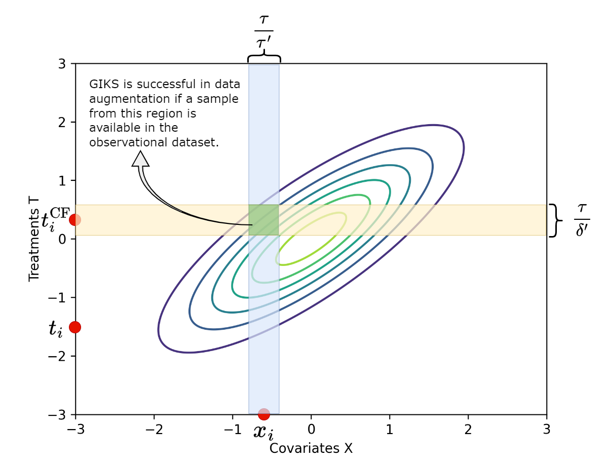
Figure 5: This figure depicts the analysis described in Section I. In the training dataset, the covariates X and treatments $T$ are jointly Gaussian with mean 0 and covariance $\begin{pmatrix}1&0.8\\ 0.8&1\end{pmatrix}$. The goal is to synthesize an outcome $\hat{y}(x_{i},t^{\text{CF}}_{i})$ such that the error in the synthesis is less than $\tau$. GIKS achieves this when the underlying observational dataset has at least one sample from the shaded green region in the middle. The shaded blue (yellow) regions in the figure represent the band of width $\frac{\tau}{\tau^{\prime}}$ ($\frac{\tau}{\delta^{\prime}}$) around $x_{i}$ ($t^{\text{CF}}_{i}$) that are considered in $D_{\text{NN}}(t^{\text{CF}}_{i})$.

I.1 GIKS addresses distribution mismatch

In this section, we aim to explain the performance of GIKS observed in the experiments by showing that the augmented samples effectively reduce the distribution mismatch between the training and test datasets while controlling the CF Error. To assess this, we compute the dependence between the covariate and treatment distributions ($D(P(\mathbf{x},T)||p(\mathbf{x})p(T))$) using the HSIC metric  (Bellot, Dhir, and Prando 2022), a kernel-based statistical independence test. The results are summarized in Table 13, where higher HSIC values indicate a stronger dependence between the $X$ and $T$ variables in the dataset.

Notably, our analysis reveals that the HSIC metric of the dataset augmented with our method is lower than that of the original dataset. This observation reinforces the effectiveness of our approach in mitigating the distribution mismatch between the training and test datasets. We also provide the corresponding $p$-values in brackets for the factual case with GIKS counterpart as the baseline, indicating statistically significant reductions in HSIC for three out of the five baseline cases. For TCGA-1 and TCGA-2, we observed large $p$-values because the factual model already exhibits strong performance in terms of the CF error, leaving limited room for improvement through our augmentation.

	CF Error		HSIC metric
	VCNet on Observational Data	VCNet on Augmented Data	VCNet on Observational Data	VCNet on Augmented Data
TCGA-0	0.19 (0.11)	0.15	2.13 (0.04)	0.57
TCGA-1	0.1 (0.08)	0.09	0.43 (0.27)	0.40
TCGA-2	0.17 (0.02)	0.13	0.41 (0.16)	0.37
IHDP	2.06 (0.0)	1.89	0.72 (0.0)	0.34
NEWS	1.09 (0.0)	1.08	0.36 (0.05)	0.35

Table 13: Comparison of the HSIC metric on the factual observational dataset and the Augmented dataset obtained by GIKS. We copy over the CF error from our main table for reference. We present the $p$ values within brackets for the factual case for the one-sided paired T test with GIKS as the baseline.

References

- Alaa and Van Der Schaar (2017) Alaa, A. M.; and Van Der Schaar, M. 2017. Bayesian inference of individualized treatment effects using multi-task gaussian processes. Advances in neural information processing systems, 30.
- Alvarez Melis and Jaakkola (2018) Alvarez Melis, D.; and Jaakkola, T. 2018. Towards Robust Interpretability with Self-Explaining Neural Networks. In Bengio, S.; Wallach, H.; Larochelle, H.; Grauman, K.; Cesa-Bianchi, N.; and Garnett, R., eds., Advances in Neural Information Processing Systems, volume 31. Curran Associates, Inc.
- Arjovsky et al. (2019) Arjovsky, M.; Bottou, L.; Gulrajani, I.; and Lopez-Paz, D. 2019. Invariant risk minimization. arXiv preprint arXiv:1907.02893.
- Bellot, Dhir, and Prando (2022) Bellot, A.; Dhir, A.; and Prando, G. 2022. Generalization bounds and algorithms for estimating conditional average treatment effect of dosage.
- Bica, Jordon, and van der Schaar (2020) Bica, I.; Jordon, J.; and van der Schaar, M. 2020. Estimating the effects of continuous-valued interventions using generative adversarial networks. Advances in Neural Information Processing Systems, 33: 16434–16445.
- Caliendo and Kopeinig (2008) Caliendo, M.; and Kopeinig, S. 2008. Some practical guidance for the implementation of propensity score matching. Journal of economic surveys, 22(1): 31–72.
- Dua and Graff (2017) Dua, D.; and Graff, C. 2017. UCI Machine Learning Repository.
- Fox and Wiens (2019) Fox, I.; and Wiens, J. 2019. Reinforcement learning for blood glucose control: Challenges and opportunities.
- Funk et al. (2011) Funk, M. J.; Westreich, D.; Wiesen, C.; Stürmer, T.; Brookhart, M. A.; and Davidian, M. 2011. Doubly robust estimation of causal effects. American journal of epidemiology, 173(7): 761–767.
- Hill (2011) Hill, J. L. 2011. Bayesian Nonparametric Modeling for Causal Inference. Journal of Computational and Graphical Statistics, 20(1): 217–240.
- Jacot, Gabriel, and Hongler (2018) Jacot, A.; Gabriel, F.; and Hongler, C. 2018. Neural tangent kernel: Convergence and generalization in neural networks. Advances in neural information processing systems, 31.
- Jesson et al. (2022) Jesson, A.; Douglas, A.; Manshausen, P.; Meinshausen, N.; Stier, P.; Gal, Y.; and Shalit, U. 2022. Scalable sensitivity and uncertainty analysis for causal-effect estimates of continuous-valued interventions. arXiv preprint arXiv:2204.10022.
- Johansson, Shalit, and Sontag (2016) Johansson, F.; Shalit, U.; and Sontag, D. 2016. Learning representations for counterfactual inference. In International conference on machine learning, 3020–3029. PMLR.
- Kallus (2020) Kallus, N. 2020. Deepmatch: Balancing deep covariate representations for causal inference using adversarial training. In International Conference on Machine Learning, 5067–5077. PMLR.
- Louizos et al. (2017) Louizos, C.; Shalit, U.; Mooij, J. M.; Sontag, D.; Zemel, R.; and Welling, M. 2017. Causal effect inference with deep latent-variable models. Advances in neural information processing systems, 30.
- Lu et al. (2020) Lu, D.; Tao, C.; Chen, J.; Li, F.; Guo, F.; and Carin, L. 2020. Reconsidering generative objectives for counterfactual reasoning. Advances in Neural Information Processing Systems, 33: 21539–21553.
- Nasery et al. (2021) Nasery, A.; Thakur, S.; Piratla, V.; De, A.; and Sarawagi, S. 2021. Training for the Future: A Simple Gradient Interpolation Loss to Generalize Along Time. Advances in Neural Information Processing Systems, 34: 19198–19209.
- Nie et al. (2021) Nie, L.; Ye, M.; Liu, Q.; and Nicolae, D. 2021. Vcnet and functional targeted regularization for learning causal effects of continuous treatments. arXiv preprint arXiv:2103.07861.
- Ozery-Flato, Thodoroff, and El-Hay (2018) Ozery-Flato, M.; Thodoroff, P.; and El-Hay, T. 2018. Adversarial Balancing for Causal Inference. ArXiv, abs/1810.07406.
- Pearl and Press (2000) Pearl, J.; and Press, C. U. 2000. Causality: Models, Reasoning, and Inference. Cambridge University Press. ISBN 9780521773621.
- Rissanen and Marttinen (2021) Rissanen, S.; and Marttinen, P. 2021. A critical look at the consistency of causal estimation with deep latent variable models. Advances in Neural Information Processing Systems, 34: 4207–4217.
- Robins, Rotnitzky, and Zhao (1994) Robins, J. M.; Rotnitzky, A.; and Zhao, L. P. 1994. Estimation of regression coefficients when some regressors are not always observed. Journal of the American statistical Association, 89(427): 846–866.
- Rubin (1973) Rubin, D. B. 1973. Matching to remove bias in observational studies. Biometrics, 159–183.
- Schwab et al. (2020) Schwab, P.; Linhardt, L.; Bauer, S.; Buhmann, J. M.; and Karlen, W. 2020. Learning counterfactual representations for estimating individual dose-response curves. In Proceedings of the AAAI Conference on Artificial Intelligence, volume 34, 5612–5619.
- Schwab, Linhardt, and Karlen (2018) Schwab, P.; Linhardt, L.; and Karlen, W. 2018. Perfect match: A simple method for learning representations for counterfactual inference with neural networks. arXiv preprint arXiv:1810.00656.
- Shalit, Johansson, and Sontag (2017) Shalit, U.; Johansson, F. D.; and Sontag, D. 2017. Estimating individual treatment effect: generalization bounds and algorithms. In International Conference on Machine Learning, 3076–3085. PMLR.
- Shi, Blei, and Veitch (2019) Shi, C.; Blei, D.; and Veitch, V. 2019. Adapting neural networks for the estimation of treatment effects. Advances in neural information processing systems, 32.
- Titsias (2009) Titsias, M. 2009. Variational learning of inducing variables in sparse Gaussian processes. In Artificial intelligence and statistics, 567–574. PMLR.
- Wang et al. (2022) Wang, X.; Lyu, S.; Wu, X.; Wu, T.; and Chen, H. 2022. Generalization bounds for estimating causal effects of continuous treatments. Advances in Neural Information Processing Systems, 35: 8605–8617.
- Yoon, Jordon, and Van Der Schaar (2018) Yoon, J.; Jordon, J.; and Van Der Schaar, M. 2018. GANITE: Estimation of individualized treatment effects using generative adversarial nets. In International Conference on Learning Representations.
- Zhang, Bellot, and Schaar (2020) Zhang, Y.; Bellot, A.; and Schaar, M. 2020. Learning overlapping representations for the estimation of individualized treatment effects. In International Conference on Artificial Intelligence and Statistics, 1005–1014. PMLR.
- Zhang et al. (2022) Zhang, Y.-F.; Zhang, H.; Lipton, Z. C.; Li, L. E.; and Xing, E. P. 2022. Exploring Transformer Backbones for Heterogeneous Treatment Effect Estimation.