DiffuserLite: Towards Real-time Diffusion Planning

Abstract

Diffusion planning has been recognized as an effective decision-making paradigm in various domains. The capability of conditionally generating high-quality long-horizon trajectories makes it a promising research direction. However, existing diffusion planning methods suffer from low decision-making frequencies due to the expensive iterative sampling cost. To address this issue, we introduce DiffuserLite, a super fast and lightweight diffusion planning framework. DiffuserLite employs a planning refinement process (PRP) to generate coarse-to-fine-grained trajectories, significantly reducing the modeling of redundant information and leading to notable increases in decision-making frequency. Our experimental results demonstrate that DiffuserLite achieves a decision-making frequency of $122$Hz ($112.7$x faster than previous mainstream frameworks) and reaches state-of-the-art performance on D4RL benchmarks. In addition, our neat DiffuserLite framework can serve as a flexible plugin to enhance decision frequency in other diffusion planning algorithms, providing a structural design reference for future works. More details and visualizations are available at project website.

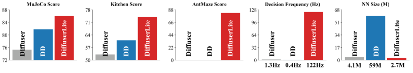
Figure 1: Performance overview. We present DiffuserLite, a lightweight framework that utilizes progressive refinement planning to reduce redundant information generation and achieve real-time diffusion planning. DiffuserLite significantly outperforms classical frameworks, Diffuser and DD, regarding scores, inference time, and model size on three popular D4RL benchmarks. It is worth noting that DiffuserLite achieves a decision-making frequency of $\bm{122}$Hz, which is $\bm{112.7}$ times higher than previous mainstream frameworks.

1 Introduction

Diffusion models (DMs) are powerful emerging generative models that demonstrate promising performance in many domains (Zhang et al., 2023; Ruiz et al., 2023; Liu et al., 2023a; Kawar et al., 2023). Motivated by their remarkable capability in complex distribution fitting and conditional sampling, in recent years, researchers have developed a series of works applying diffusion models in RL (Reinforcement Learning) (Zhu et al., 2023b). DMs play various roles in these decision-making tasks, such as acting as planners to make better decisions from a long-term perspective (Janner et al., 2022; Ajay et al., 2023; Dong et al., 2023; Ni et al., 2023; Du et al., 2023), serving as policies to support complex multimodal distributions (Pearce et al., 2023a; Wang et al., 2023; Chi et al., 2023), and working as data synthesizers to generate synthetic data for assisting RL training (Lu et al., 2023; Yu et al., 2023; He et al., 2023a), etc. Among these roles, diffusion planning is the most widely applied paradigm (Zhu et al., 2023b).

Unlike autoregressive planning in previous model-based RL approaches (Hafner et al., 2019; Thuruthel et al., 2019; Hansen et al., 2022), diffusion planning avoids severe compounding errors by directly generating the entire trajectory rather than one-step transition (Zhu et al., 2023b). Furthermore, its powerful conditional generation capability allows planning at the trajectory level without being limited to stepwise shortsightedness. The diffusion planning paradigm has achieved state-of-the-art performance in various offline decision-making tasks, including single-agent RL (Li et al., 2023), multi-agent RL (Zhu et al., 2023a), meta RL (Ni et al., 2023), and more.

One key issue diffusion planning faces is the expensive iterative sampling cost. As depicted in Figure 1, the decision-making frequencies (actions per second) of two prominent diffusion planning frameworks, Diffuser (Janner et al., 2022) and Decision Diffuser (DD) (Ajay et al., 2023), are recorded as $1.3$Hz and $0.4$Hz, respectively. Such decision frequencies fall short of meeting the requirements of numerous real-world applications, such as real-time robot control (Tai et al., 2018) and game AI (Pearce et al., 2023b). The slow decision speed of diffusion planning is primarily attributed to fitting a denoising process for a long-horizon trajectory distribution. This process requires a heavy neural network backbone and multiple forward passes for denoising. However, we have observed that the detailed information at the long horizon generated by current diffusion planning is redundant. As shown in Figure 2, a motivation example in Antmaze, the disparities between plans increase as the horizon grows, leading to poor consistency between plans in consecutive steps. In addition, agents often struggle to reach the planned distant state in practice. These facts indicate that while long-horizon planning helps improve foresight, details in distinct parts become increasingly redundant, and the closer details are more crucial. Ignoring modeling these redundant parts in the diffusion planning process will significantly reduce the complexity of the trajectory distribution to be fitted, making it possible to build a fast and lightweight diffusion planning framework.

Motivated by this, we propose to build a plan refinement process (PRP) to speed up diffusion planning. First, we perform “rough” planning, where jumpy planning is executed, only considering the states at intervals that are far apart and ignoring other individual states. Then, we refine a small portion of the plan, focusing on the steps closer to the current time. By doing so, we fill in the execution details between two states far apart, gradually refining the plan to the step level. This approach has three significant advantages. First, it reduces the length of the sequences generated by diffusion, simplifying the complexity of the probability distribution to be fitted. Second, it significantly reduces the search space of the plan, making it easier for the planner to find better trajectories. Additionally, since only the first action of each step is executed, rough planning of steps further away does not have a noticeable impact on performance.

Our proposed diffusion planning framework, which we call DiffuserLite, is simple, fast, and lightweight. Our experiments have demonstrated the effectiveness of PRP, significantly increasing decision-making frequency (action decided per second) while achieving state-of-the-art performance. Moreover, it can be easily adapted to other existing diffusion planning methods. In summary, our contributions are as follows:

• We introduce the plan refinement process (PRP) for coarse-to-fine-grained trajectory generation, reducing the modeling of redundant information.

• We introduce DiffuserLite, a lightweight diffusion planning framework, which significantly increases decision-making frequency by employing PRP.

• DiffuserLite is a simple and flexible plugin that can be easily combined with other diffusion planning algorithms.

• DiffuserLite achieves a super high decision-making frequency ($122$Hz, $112.7$x faster then previous mainstream frameworks) and state-of-the-art performance on multiple benchmarks in D4RL.

2 Preliminaries

Problem Setup: Consider a system governed by discrete-time dynamics $o_{t+1}=f(o_{t},a_{t})$ at state $o_{t}$ given an action $a_{t}$. A trajectory $\bm{x}=[x_{0},\cdots,x_{T-1}]$ can be a sequence of states $x_{t}=o_{t}$ or state-action pairs $x_{t}=(o_{t},a_{t})$, where $T$ is the planning horizon. Each trajectory can be mapped to a unique property $\bm{c}$. Diffusion planning aims to find a trajectory that exhibits a property that is closest to the target:

$$\bm{x}^{*}=\underset{\bm{x}}{\arg\min}~{}d(\mathcal{C}(\bm{x}),\bm{c}_{\text{target}})$$ (1)

where $d$ is a certain distance metric, $\mathcal{C}$ is a critic that maps a trajectory to the property it exhibits, and $c_{\text{target}}$ is the target property. An action $a_{t}$ to be executed is then extracted from the selected trajectory (state-action sequences) or predicted by inverse dynamics model $a_{t}=h(o_{t},o_{t+1})$ (state-only sequences). In the context of offline RL, it is a common choice to define the property as the corresponding cumulative reward $\mathcal{C}(\bm{x})=\sum_{t=0}^{T-1}r(o_{t},a_{t})$ in previous works (Janner et al., 2022; Ajay et al., 2023).

Diffusion Models assume an unknown trajectory distribution $q_{0}(\bm{x}_{0})$, DMs define a forward process $\{x_{s}\}_{s\in[0,S]}$ with $S>0$. Starting with $\bm{x}_{0}$, Kingma et al. (2021) proved that one can obtain any $\bm{x}_{s}$ by solving the following stochastic differential equation (SDE):

$${\rm d}\bm{x}_{s}=f(s)\bm{x}_{s}{\rm d}s+g(s){\rm d}\bm{w}_{s},~{}\bm{x}_{0}\sim q_{0}(\bm{x}_{0})$$ (2)

where $\bm{w}_{s}$ is the standard Wiener process, and $f(s)={\rm d}\log\alpha_{s}/{\rm d}s$, $g^{2}(s)={\rm d}\sigma_{s}^{2}/{\rm d}s-2\sigma_{s}^{2}{\rm d}\log\alpha_{s}/{\rm d}s$. Values of $\alpha_{s},\sigma_{s}\in\mathbb{R}^{+}$ depend on the noise schedule but keep the signal-to-noise-ratio (SNR) $\alpha^{2}_{s}/\sigma^{2}_{s}$ strictly decreasing (Kingma et al., 2021). While this SDE transforms $q_{0}(\bm{x}_{0})$ into a noise distribution $q_{S}(\bm{x}_{S})=\mathcal{N}(\bm{0},\bm{I})$, one can reconstruct trajectories from the noise by solving the reverse process of Equation 2. Song et al. (2021b) proved that solving its associated probability flow ODE can support faster sampling:

$$\frac{{\rm d}\bm{x}_{s}}{{\rm d}s}=f(s)\bm{x}_{s}-\frac{1}{2}g^{2}(s)\nabla_{\bm{x}}\log q_{s}(\bm{x}_{s}),~{}\bm{x}_{S}\sim q_{S}(\bm{x}_{S})$$ (3)

in which score function $\nabla_{\bm{x}}\log q_{s}(\bm{x}_{s})$ is the only unknown term and estimated by a neural network $-\bm{\epsilon}_{\theta}(\bm{x}_{s},s)/\sigma_{s}$ in practice. The parameter $\theta$ is optimized by minimizing the following objective:

$$\mathcal{L}(\theta)=\mathbb{E}_{q_{0}(\bm{x}_{0}),q(\bm{\epsilon}),s}[||\bm{\epsilon}_{\theta}(\bm{x}_{s},s)-\bm{\epsilon}||^{2}_{2}]$$ (4)

where $\bm{\epsilon}\sim q(\bm{\epsilon})=\mathcal{N}(\bm{0},\bm{I})$, $\bm{x}_{s}=\alpha_{s}\bm{x}_{0}+\sigma_{s}\bm{\epsilon}$. Various ODE solvers can be employed to solve Equation 3, such as the Euler solver (Atkinson, 1989), RK45 solver (Dormand & Prince, 1980), DPM solver (Lu et al., 2022), etc.

Conditional Sampling helps to generate trajectories exhibiting certain properties in a priori. There are two main approaches: classifier-guidance (CG) (Dhariwal & Nichol, 2021) and classifier-free-guidance (CFG) (Ho & Salimans, 2021). CG involves training an additional classifier $\log p_{\phi}(c|\bm{x}_{s},s)$ to predict the log probability that a noisy trajectory exhibits a given property. The gradients from this classifier are then used to guide the solver:

$$\tilde{\bm{\epsilon}_{\theta}}(\bm{x}_{s},s,c):=\bm{\epsilon}_{\theta}(\bm{x}_{s},s)-w\cdot\sigma_{s}\nabla_{\bm{x}_{s}}\log p_{\phi}(c|\bm{x}_{s},s)$$ (5)

CFG does not require training an additional classifier but uses a conditional noise predictor to guide the solver.

$$\tilde{\bm{\epsilon}_{\theta}}(\bm{x}_{s},s,\bm{c}):=w\cdot\bm{\epsilon}_{\theta}(\bm{x}_{s},s,\bm{c})+(1-w)\cdot\bm{\epsilon}_{\theta}(\bm{x}_{s},s)$$ (6)

Increasing the value of guidance strength $w$ leads to more property-aligned generation, but also decreases the legality (Dong et al., 2023).

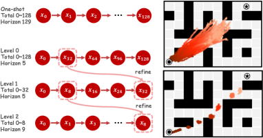
Figure 2: Comparison of one-shot planning (top) and PRP (down) on Antmaze. The former directly generates plans with a temporal horizon of $129$. The latter consists of three coarse to fine-grained levels with temporal horizons of $0$-$128$, $0$-$32$, and $0$-$8$, and temporal jumps of $32$, $8$, and $1$, respectively. The visualization in the figure illustrates the x-y coordinates of $100$ plans. It can be observed that one-shot planning exhibits a significant amount of redundant information and a large search space. In contrast, PRP demonstrates better plan consistency and a smaller search space.

3 Efficient Planning via Refinement

Diffuser (Janner et al., 2022) and DD (Ajay et al., 2023) are two pioneering frameworks, and a vast amount of diffusion planning research has been built upon them (Liang et al., 2023; Lee et al., 2023; Zhou et al., 2023). Although the design details differ, the two can be unified into a single paradigm. At each decision-making step, multiple candidate trajectories, starting from the current state, are conditionally sampled by the diffusion model. A critic is then used to select the optimal one that exhibits the closest property to the target. Finally, the action to be executed is extracted from it. However, this paradigm relies on multiple forwarding complex neural networks, resulting in extremely low decision-making frequencies (typically $1$-$10$Hz, or even less than $1$Hz), severely hindering its real-world deployment.

The fundamental reason can be the need for highly complex neural networks to fit the complex trajectory distributions (Zhu et al., 2023b). Although some works have explored using advanced ODE solvers to reduce the sampling steps to around $3$ (Dong et al., 2023; He et al., 2023c), the time consumption of network forwarding is still unacceptable. However, we notice that ignoring some redundant distant parts of the generated plan can be a possible solution to address the issue. As shown in Figure 2, the disparities between plans increase as the horizon grows, leading to poor consistency between the plans selected in consecutive steps. Besides, agents often struggle to actually reach the distant states given by a plan in practice. Both facts indicate that terms in distant parts of a plan become increasingly redundant, whereas the closer parts are more crucial.

In light of these findings, we aim to develop a progressive refinement planning (PRP) process. This process initially plans a rough trajectory consisting of only key points spaced at equal intervals and then progressively refines the first interval by generative interpolating. Specifically, our proposed PRP consists of $L$ planning levels. At each level $l\in\{0,1,\cdots,L-1\}$, starting from the known first term $x_{0}$, DMs plan rough trajectories $\bm{x}_{0:H_{l}:I_{l}}$ with temporal horizon $H_{l}$ and temporal jump $I_{l}$. Then, the planned first key point $x_{I_{l}}$ is passed to the next level as its terminal:

$$\bm{x}_{0:H_{l}:I_{l}}: =\left[x_{0},x_{I_{l}},x_{2I_{l}}\cdots,x_{H_{l}-1}\right]$$ (7)

$$\bm{x}_{0:H_{l+1}:I_{l+1}}: =\left[x_{0},x_{I_{l+1}},x_{2I_{l+1}},\cdots,x_{H_{l+1}-1}\right]$$

$$x_{I_{l}} =x_{H_{l+1}-1}$$

By this design, only the first planned intervals are refined in the next level, and the other redundant details are all ignored. The progressive refinement is conducted until the last level in which $I_{L-1}=1$ to extract an action. To support conditional sampling for each level, we define the property of a rough trajectory $\bm{x}_{0:H_{l}:I_{l}}$ as the property expectation over the distribution of all its completed trajectories $\mathcal{X}(\bm{x}_{0:H_{l}:I_{l}})$:

$$\mathcal{C}(\bm{x}_{0:H_{l}:I_{l}}):=\mathbb{E}_{\bm{x}\sim\mathcal{X}(\bm{x}_{0:H_{l}:I_{l}})}[\mathcal{C}(\bm{x})]$$ (8)

PRP ensures that long-term planning maintains foresight while alleviating the burden of modeling redundant information. As a result, it greatly contributes to reducing model size and improving planning efficiency:

Simplifying the fitted distribution of DMs. The absence of redundant details in PRP allows for a significant reduction in the complexity of the fitted distribution at each level. This reduction in complexity enables us to utilize a lighter neural network backbone, shorter network input sequence lengths, and a reduced number of denoising steps.

Reducing the plan-search space. Key points generated at former levels often sufficiently reflect the quality of the entire trajectory, which allows the planner to focus more on finding distant key points and planning actions for the immediate steps, reducing search space and complexity.

Algorithm 1 DiffuserLite Training

  Input: number of planning levels $L$, temporal horizon $H_{l}$, temporal jump $I_{l}$ and noise estimators $\bm{\epsilon}_{\theta_{l}}$ for each level $l\in\{0,1,\cdots,L-1\}$, dataset $\mathcal{D}=\{\bm{x}\}$, where $\bm{x}$ is the sequence of state-action pairs, critic $\mathcal{C}$, diffusion steps $T$, condition mask probability $1-p$;

  while not done do

     sample a batch of $(\bm{x},\mathcal{C}(\bm{x}))$ from dataset $\mathcal{D}$

     for $l=0$ to $L-1$ do

        extract $\bm{x}_{0,H_{l},1}$ and $\bm{x}_{0,H_{l},I_{l}}$ from $\bm{x}$

        $\hat{\mathcal{C}}({\bm{x}_{0,H_{l},I_{l}})}\leftarrow\mathcal{C}(\bm{x}_{0,H_{l},1})$

        sample $s_{l}\sim\text{Uniform}(T)$, $\bm{\epsilon}_{l}\sim\mathcal{N}(\bm{0},\bm{I})$

        first state of $\bm{\epsilon}_{l}\leftarrow$ first state of $\bm{x}_{0,H_{l},I_{l}}$

        if $l>0$ then

           last state of $\bm{\epsilon}_{l}\leftarrow$ last state of $\bm{x}_{0,H_{l},I_{l}}$

        end if

        $\bm{x}^{s}_{0:H_{l}:I_{l}}\leftarrow\alpha_{s}\bm{x}_{0:H_{l}:I_{l}}+\sigma_{s}\bm{\epsilon}_{l}$

        update $\theta_{l}$ by minimizing $||\bm{\epsilon}_{\theta_{l}}(\bm{x}^{s}_{0:H_{l}:I_{l}},s,\mathcal{C}(\bm{x}_{0:H_{l}:I_{l}}))-\bm{\epsilon}||^{2}$ with probability $p$ else $||\bm{\epsilon}_{\theta_{l}}(\bm{x}^{s}_{0:H_{l}:I_{l}},s))-\bm{\epsilon}||^{2}$

     end for

  end while

4 A Lite Architecture for Real-time Diffusion Planning

Employing PRP results in a new lightweight architecture for diffusion planning, which we refer to as DiffuserLite. DiffuserLite can reduce the complexity of the fit distribution and significantly increase the decision-making frequency, achieving $\sim 100$Hz on average for the need of real-time control. We present the architecture overview in LABEL:fig:3, provide pseudocode for both training and inference in Algorithm 1 and Algorithm 2, and discuss detailed design choices in this section.

Diffusion model for each level: We train $L$ diffusion models for all levels to generate state-only sequences. We employ DiT (Peebles & Xie, 2022) as the noise predictor backbone, instead of the more commonly used UNet (Ronneberger et al., 2015) due to the significantly reduced length of the generated sequences in each level (typically around $5$). This eliminates the need for $1$D convolution to extract local temporal features. To adapt the DiT backbone for temporal generation, we make minimal structural adjustments following (Dong et al., 2023). For conditional sampling, we utilize CFG instead of CG, as the slow gradient computation process of CG reduces the frequency of decision making. During the training phase, at each gradient step, we sample a batch of $H_{0}$-length trajectories, slice each of them into $L$ sub-trajectories $[\bm{x}_{0:H_{0}:1},\cdots,\bm{x}_{0:H_{L-1}:1}]$, evaluate their properties $\mathcal{C}(\bm{x}_{0,H_{l},1})$ as an estimation of $\mathcal{C}(\bm{x}_{0:H_{l}:I_{l}})$, and then slice the sub-trajectories into evenly spaced training samples $\bm{x}_{0:H_{l}:I_{l}}$ for training the diffusion models. During the inference phase, as shown in the upper half of LABEL:fig:3, the diffusion model at each level generates multiple candidate plans for the critic to select the optimal one.

Critic and property design: The Critic $\mathcal{C}$ in DiffuserLite plays two important roles: providing generation conditions during the diffusion training process and selecting the optimal plan from the candidates generated by the diffusion model during inference. In the context of Offline RL, both Diffuser and DD adopt the cumulative reward of a trajectory as the condition

$$\mathcal{C}(\bm{x})=\sum_{t=0}^{H-1}r(o_{t},a_{t}),$$ (9)

where $H$ is the temporal horizon. This design allows rewards from the offline RL dataset to be utilized as a ground-truth critic for acquiring generation conditions during training. During inference, an additional reward function needs to be trained to serve as the critic. The critic then helps select the plan that maximizes the cumulative reward, as depicted in the lower part of LABEL:fig:3. However, this design poses challenges in tasks with sparse rewards, as it can confuse diffusion models when distinguishing better-performing trajectories, especially for short-horizon plans. To address this challenge, we introduce an option to use the sum of discounted rewards and the value of the last state as an additional property design:

$$\mathcal{C}(\bm{x})=\sum_{t=0}^{H-2}\gamma^{t}r(o_{t},a_{t})+\gamma^{H-1}V(o_{H-1}),$$ (10)

where $V(o_{t})=\max\mathbb{E}_{\pi}[\sum_{\tau=t}^{\infty}\gamma^{\tau-t}r_{\tau}]$ represents the optimal value function (Sutton & Barto, 1998) and can be estimated by a neural network through various offline RL methods. This critic can be used the same way as the previous one during training and inference. In the context of other domains, properties can be flexibly designed as needed, as long as the critic $\mathcal{C}$ can evaluate trajectories of variable lengths. It is worth noting that diffusion planning works widely support this flexibility. In addition, it is even possible to skip the critic selection during inference, which is equivalent to using a uniform critic, as utilized in DD.

Action extraction: After obtaining the optimal trajectory from the last level through critic selection, we utilize an additional inverse dynamic model $a_{t}=h(o_{t},o_{t+1})$ to extract the action to be executed. This approach is suggested in (Ajay et al., 2023).

Further speedup with rectified flow: DiffuserLite aims to achieve real-time diffusion planning to support its application in real-world scenarios. Therefore, we introduce Rectified flow (Liu et al., 2023b) for further increasing the decision-making frequency. Rectified flow, an ODE on the time interval $[0,1]$, causalizes the paths of linear interpolation between two distributions. If we define the two distributions as trajectory distribution and standard Gaussian, we can directly replace the Diffusion ODE with rectified flow to achieve the same functionality. The most significant difference is that rectified flow learns a straight-line flow and can continuously straighten the ODE through reflow. This straightness property allows for consistent and stable gradients throughout the flow, enabling the generation of trajectories with very few sampling steps (in our experiments, we found that one-step sampling is sufficient to produce good results). We consider rectified flow an optional backbone for cases that prioritize decision frequency. In Appendix B, we offer comprehensive explanations of trajectory generation and training with rectified flow.

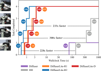
Figure 4: Runtime and performance comparison in Kitchen. The y-axis represents the number of completed tasks (maximum of $4$), and the x-axis represents the required wall-clock time. The numbers inside the circles represent the corresponding task success rates. All data are averaged over 250 rollouts. DiffuserLite demonstrates significant decision-speed advantages across all backbones. In particular, the R2 version shows a speed improvement of 200-300 times compared to DD. Additionally, DiffuserLite also exhibits significant advantages in task success rate.

5 Experiments

Table 1: The time consumption per step and frequency tested in D4RL. All results are obtained over 5 random seeds. The improved DiffuserLite can achieve an average decision frequency of about 100 Hz, which meets the requirements of real-time inference.

Environment	Metric	Diffuser	DD	DiffuserLite-D	DiffuserLite-R1	DiffuserLite-R2
MuJoCo	Runtime (s)	$0.665$	$2.142$	$0.015$	$0.013$	$0.005$
	Frequency (Hz)	$1.5$	$0.47$	$68.2$	$79.7$	$200.7$
Kitchen	Runtime (s)	$0.790$	$2.573$	$0.017$	$0.015$	$0.097$
	Frequency (Hz)	$1.3$	$0.4$	$58.7$	$66.0$	$103.2$
Antmaze	Runtime (s)	$0.791$	$2.591$	$0.027$	$0.015$	$0.098$
	Frequency (Hz)	$1.3$	$0.39$	$37.3$	$65.7$	$101.7$
Average Runtime (s)		$0.749$	$2.435$	$\bm{0.020}$	$\bm{0.014}$	$\bm{0.008}$

In this paper, we explore the performance of the DiffuserLite on a variety of decision-making tasks on D4RL benchmark (Fu et al., 2020). Through the experiments, we aim to answer the following research questions (RQs): 1) To what extent can DiffuserLite reduce the runtime cost? 2) What is the performance of DiffuserLite in offline RL tasks? 3) Can DiffuserLite be used as a flexible plugin in other diffusion planning algorithms? 4) What is the role of each components in the DiffuserLite?

5.1 Experimental Setup

Benchmarks: We evaluate the algorithm performance on three popular offline RL domains: Gym-MuJoCo (Brockman et al., 2016), Franka Kitchen (Gupta et al., 2020), and Antmaze (Fu et al., 2020) We train all models using publicly available D4RL datasets (see Section A.1 for further details about each benchmark domain).

Baselines: Our comparisons include the basic imitation learning algorithm BC, existing offline RL methods CQL (Kumar et al., 2020) and IQL (Kostrikov et al., 2022), as well as two pioneering diffusion planning frameworks, Diffuser (Janner et al., 2022) and DD (Ajay et al., 2023). Additionally, we compare with a state-of-the-art algorithm, HDMI (Li et al., 2023), which is improved based on DD. (Further details about each baseline and the sources of performance results for each baseline across the experiments are presented in Section A.2).

Backbones: As mentioned in Section 4, we implement three variations of DiffuserLite, based on different backbones: 1) diffusion model, 2) rectified flow, and 3) rectified flow with an additional reflow step. These variations will be used in subsequent experiments and indicated by the suffixes D, R1, and R2, respectively. All backbones utilize $3$ levels, with a total temporal horizon of $129$ in MuJoCo and Antmaze, and $49$ in Kitchen. For more details about the hyperparameters selection for DiffuserLite, please refer to Appendix C.

Computing Power: All runtime results across our experiments are obtained by running the code on a server equipped with an Intel(R) Xeon(R) Gold 6326 CPU @ 2.90GHz and an NVIDIA GeForce RTX3090.

5.2 Runtime Cost (RQ1)

The primary objective of DiffuserLite is to increase the decision-making frequency. Therefore, we first test the wall-clock runtime cost of DiffuserLite under three different backbones, compared to two pioneering frameworks Diffuser and DD, to determine the extent of the advantage gained. We present the test results in Table 1, which shows that the runtime cost of DiffuserLite with D, R1, and R2 backbones is only $1.23\%$, $0.89\%$, and $0.51\%$ of the average runtime cost of Diffuser and DD, respectively. The remarkable improvement in decision-making frequency has not harmed its performance. As shown in Figure 4, compared to the average success rates of Diffuser (purple line) and DD (grey line) on four Franka Kitchen sub-tasks, DiffuserLite improves them by $[41.5\%,56.2\%,55.3\%,8.7\%]$, respectively, while being $200\sim 300$ times faster. These improvements are attributed to ignoring redundant information in PRP, which reduces the complexity of the distribution that the backbone generative model needs to fit, allowing us to employ a light neural network backbone and use fewer sampling steps to conduct perfect-enough planning. Its success in Franka Kitchen, a realistic robot manipulation scenario, also reflects its potential application in real-world settings.

5.3 Performance (RQ2)

Table 2: The performance in D4RL in terms of normalized average returns. Results for DiffuserLite correspond to the mean and standard error over $5$ random seeds. We detail the sources for the performance of prior methods in Section A.2. Following Janner et al. (2022), we emphasize in bold scores within $5$ percent of the maximum per task ($\geq 0.95\cdot\text{max}$).

Dataset	Environment	BC	CQL	IQL	Diffuser	DD	HDMI	DiffuserLite-D	DiffuserLite-R1	DiffuserLite-R2
Medium-Expert	HalfCheetah	$55.2$	$\bm{91.6}$	$86.7$	$79.8$	$\bm{90.6}$	$\bm{92.1}$	$88.5\pm 0.4$	$\bm{90.8\pm 0.9}$	$84.0\pm 2.9$
	Hopper	$52.5$	$105.4$	$91.5$	$107.2$	$\bm{111.8}$	$\bm{113.5}$	$\bm{111.6\pm 0.2}$	$\bm{110.3\pm 0.3}$	$\bm{110.1\pm 0.5}$
	Walker2d	$\bm{107.5}$	$\bm{108.8}$	$\bm{109.6}$	$\bm{108.4}$	$\bm{108.8}$	$\bm{107.9}$	$\bm{107.1\pm 0.6}$	$\bm{106.4\pm 0.3}$	$\bm{106.1\pm 0.7}$
Medium	HalfCheetah	$42.6$	$44.0$	$\bm{47.4}$	$44.2$	$\bm{49.1}$	$\bm{48.0}$	$\bm{48.9\pm 1.1}$	$\bm{48.6\pm 0.7}$	$45.3\pm 0.5$
	Hopper	$52.9$	$58.5$	$66.3$	$58.5$	$79.3$	$76.4$	$\bm{100.9\pm 1.1}$	$\bm{99.5\pm 0.7}$	$\bm{96.8\pm 0.3}$
	Walker2d	$75.3$	$72.5$	$78.3$	$79.7$	$82.5$	$79.9$	$\bm{88.8\pm 0.6}$	$\bm{85.1\pm 0.5}$	$83.7\pm 1.0$
Medium-Replay	HalfCheetah	$36.6$	$\bm{45.5}$	$\bm{44.2}$	$42.2$	$39.3$	$\bm{44.9}$	$41.6\pm 0.4$	$42.9\pm 0.4$	$39.6\pm 0.4$
	Hopper	$18.1$	$95.0$	$94.7$	$\bm{96.8}$	$\bm{100.0}$	$\bm{99.6}$	$\bm{96.6\pm 0.3}$	$\bm{97.8\pm 1.3}$	$93.2\pm 0.7$
	Walker2d	$26.0$	$77.2$	$73.9$	$61.2$	$75.0$	$80.7$	$\bm{90.2\pm 0.5}$	$84.6\pm 1.7$	$78.2\pm 1.7$
Average		$51.9$	$77.6$	$77$	$75.3$	$\bm{81.8}$	$\bm{82.6}$	$\bm{86.0}$	$\bm{85.1}$	$\bm{81.9}$
Mixed	Kitchen	$51.5$	$52.4$	$51.0$	$50.0$	$65$	$69.2$	$\bm{73.6\pm 0.7}$	$\bm{71.9\pm 1.4}$	$64.8\pm 1.8$
Partial	Kitchen	$38.0$	$50.1$	$46.3$	$56.2$	$57$	$-$	$\bm{74.4\pm 0.6}$	$69.9\pm 0.7$	$\bm{71.4\pm 1.2}$
Average		$44.8$	$51.3$	$48.7$	$53.1$	$61.0$	$-$	$\bm{74.0}$	$\bm{70.9}$	$68.1$
Play	Antmaze-Medium	$0.0$	$65.8$	$65.8$	$0.0$	$0.0$	$-$	$78.0\pm 2.2$	$\bm{88.0\pm 2.2}$	$\bm{88.8\pm 3.2}$
	Antmaze-Large	$0.0$	$20.8$	$42.0$	$0.0$	$0.0$	$-$	$\bm{72.0\pm 6.2}$	$\bm{72.4\pm 2.3}$	$\bm{69.4\pm 6.5}$
Diverse	Antmaze-Medium	$0.8$	$67.3$	$73.8$	$0.0$	$0.0$	$-$	$\bm{92.4\pm 3.2}$	$\bm{89.2\pm 2.0}$	$\bm{87.6\pm 2.0}$
	Antmaze-Large	$0.0$	$20.5$	$30.3$	$0.0$	$0.0$	$-$	$68.0\pm 2.8$	$\bm{80.4\pm 5.1}$	$75.2\pm 3.5$
Average		$0.2$	$43.6$	$53.0$	$0.0$	$0.0$	$-$	$77.6$	$\bm{82.5}$	$\bm{80.3}$
Runtime per action (second)		$-$	$-$	$-$	$0.749$	$2.435$	$-$	$\bm{0.020}$	$\bm{0.014}$	$\bm{0.008}$

Then, we evaluate DiffuserLite on various popular domains in D4RL to test how well it can maintain its performance when significantly increasing the decision-making frequency. We present all test results in Table 2, and provide detailed descriptions of the sources of all baseline results in Section A.2. Results for DiffuserLite represent the mean and standard error over $5$ random seeds. We surprisingly find that DiffuserLite achieves significant performance improvements across all benchmarks while keeping high decision-making frequency. This advantage is particularly pronounced in Kitchen and Antmaze environments, indicating that the structure of DiffuserLite enables more accurate and efficient planning in long-horizon tasks, thus yielding greater benefits. In the MuJoCo environments, we observe that DiffuserLite does not exhibit a significant advantage over the baselines on “medium-expert” datasets but shows clear advantages on “medium” and “medium-replay” datasets. We attribute this to the PRP planning structure, which does not require one-shot generation of a consistent long trajectory, but explicitly demands stitching. This allows for better utilization of high-quality segments in low-quality datasets, leading to improved performance.

5.4 Flexible Plugin (RQ3)

Table 3: Integrate with DiffuserLite to accelerate a behavior-customizing diffusion planning algorithm. We refer to AlignDiff with DiffuserLite plugin as AlignDiff-Lite. A larger value of the area metric indicates a stronger alignment capability. AlignDiff-Lite greatly increases decision-making frequency, while only experiencing a small performance drop.

Metric	GC	AlignDiff	AlignDiff-Lite
MAE Area	$0.319\pm 0.005$	$0.621\pm 0.023$	$0.601\pm 0.018$ ($3.2\%\downarrow$)
Frequency (Hz)	$-$	$6.9$	$45.5$ ($560\%\uparrow$)

To test the capability of DiffuserLite as a flexible plugin to support other diffusion planning algorithms, we select AlignDiff (Dong et al., 2023) for non-reward-maximizing environments, and integrate it with the DiffuserLite plugin, referred to as AlignDiff-Lite. AlignDiff aims to customize the agent’s behavior to align with human preferences and introduces an MAE area metric to measure this alignment capability (refer to Section A.3 for more details), where a larger value indicates a stronger capability. So, we test the alignment capability of AlignDiff-Lite and present the results in Table 3. The results show that AlignDiff-Lite achieves a $560\%$ improvement in decision-making frequency compared to AlignDiff, while only experiencing a small performance drop of $3.2\%$. This indicates that integrating DiffuserLite has the potential to accelerate diffusion planning in various domains, empowering its applications.

5.5 Ablations (RQ4)

Has the last level (short horizon) of DiffuserLite already performed well in decision making? This is equivalent to the direct use of the shorter planning horizon. If it is true, key points generated by former levels may not have an impact, making PRP meaningless. To address this question, we conduct tests using a one-level DiffuserLite with the same temporal horizon as the last level of the default model, referred to as Lite w/ only last level. The results are presented in Table 4, column $2$. The notable performance drop demonstrates the importance of a long-enough planning horizon.

Can decision-making be effectively accomplished without progressive refinement planning (PRP)? To address this question, we conduct tests using a one-level DiffuserLite with the same temporal horizon as the default model, referred to as Lite w/o PRP. This model only supports one-shot generation at the inference phase. We also test a “smaller” DD with the same network parameters and sampling steps as DiffuserLite, to verify whether one can speed up DD by simply reducing the parameters, referred to as DD-small. The results are presented in Table 4, column $3$-$4$. The large standard deviation and the significant performance drop provide strong evidence for the limitations of one-shot generation planning, having difficulties in modeling the distribution of detailed long-horizon trajectories. However, DiffuserLite can maintain high performance with fast decision-making frequency due to its lite architecture and simplified fitted distribution.

How to choose between generation conditions with or without values? DiffuserLite offers two optional generation conditions, resulting in two different critics, as introduced in Section 4. To determine the suitability of these two approaches in different tasks, we conduct ablation experiments and present the results in Table 5. We find that in dense reward tasks, such as Hopper and HalfCheetah, the performance of both conditions is nearly identical. However, in sparse reward scenarios, such as Kitchen and Antmaze, the use of values demonstrates a significant advantage. We present a visual comparison in Antmaze in Figure 5, which shows $100$ generated plans. With a pure-rewards condition, it is difficult to discern the endpoint location, as the planner often desires to stop at a certain point on the map. However, when using values, the planner indicates a desire to move towards the endpoint. This suggests that sparse reward tasks are prone to confusing the conditional generative model, leading to poor planning. The introduction of value-assisted guidance can address this issue.

Table 4: Ablation tests conducted to examine the effectiveness of PRP. Lite w/ only last level and Lite w/o PRP are two ablated versions of DiffuserLite, while DD-small is a version of DD that uses the same network parameters and sampling steps as DiffuserLite. All results are obtained over $5$ seeds. The varying degrees of performance drop observed in each experiment highlight the importance of PRP.

Environment	Oracle	Lite w/	Lite w/o	DD
		only last level	PRP	small
Hopper-me	$111.6\pm 0.2$	$27.8\pm 10.2$	$96.6\pm 1.0$	$67.9\pm 24.7$
Hopper-m	$100.9\pm 1.1$	$19.4\pm 2.0$	$66.4\pm 20.2$	$16.7\pm 8.0$
Hopper-mr	$96.6\pm 0.3$	$2.0\pm 0.2$	$62.5\pm 31.3$	$1.0\pm 0.4$
Average	$103.1$	$16.4$ $(84.1\%\downarrow)$	$75.2$ $(27.1\%\downarrow)$	$28.5$ $(72.3\%\downarrow)$
Kitchen-m	$73.6\pm 0.7$	$48.2\pm 1.4$	$26.9\pm 1.0$	$0.0\pm 0.0$
Kitchen-p	$74.4\pm 0.6$	$38.6\pm 3.1$	$23.9\pm 0.5$	$1.8\pm 0.8$
Average	$74.0$	$43.4$ $(41.3\%\downarrow)$	$25.4$ $(65.7\%\downarrow)$	$0.8$ $(98.8\%\downarrow)$

Table 5: Performance of DiffuserLite using conditions with or without values. Present only average performance on varying-quality datasets, which are obtained over $5$ seeds.

Condition	Hopper	HalfCheetah	Kitchen	Antmaze
w/   Value	$103.6$	$60.7$	$74.0$	$77.6$
w/o Value	$103.1$	$59.7$	$54.1$	$19.7$

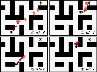
Figure 5: Visual comparison of DiffuserLite using conditions with (upper) or without (lower) values. It displays $100$ plans generated at the current state, where darker colors indicate closer proximity to the current state, and lighter colors indicate further. With the pure-rewards condition, we can observe that the planned states in lighter colors tend to cluster together at a certain point on the map, indicating the planner tries to stop at that non-endpoint. However, with the introduction of values, the planner can make correct long-term plans that lead to the endpoint.

6 Related Works

Diffusion models are a type of score-matching-based generative model (Song et al., 2021b). Two pioneering frameworks Janner et al. (2022) and Ajay et al. (2023) were the first to attempt using diffusion models for trajectory generation and planning in decision-making tasks. Based on these two frameworks, diffusion planning has been continuously improved and applied to various decision domains (Ni et al., 2023; Du et al., 2023; Zhu et al., 2023a; Dong et al., 2023; He et al., 2023b; Lee et al., 2023; Jiang et al., 2023). However, long-horizon estimation and prediction often suffer from potential exponentially increasing variance concerning the temporal horizon, called the “curse of horizon” (Ren et al., 2021). To address this, HDMI (Li et al., 2023) is the first algorithm that proposed a hierarchical decision framework to generate sub-goals at the upper level and reach goals at the lower level, achieving improvements in long-horizon tasks. However, HDMI is limited by cluster-based dataset pre-processing to obtain high-quality sub-goal data for upper training. Another concurrent work, HD-DA (Chen et al., 2024) introduces a similar hierarchical structure and allows the high-level diffusion model to automatically discover sub-goals from the dataset, achieving better results. However, the motivation behind DiffuserLite is completely different, which aims to increase the decision-making frequency of diffusion planning. Also, DiffuserLite allows for more hierarchy levels and refines only the first interval of the previous layer using PRP. Since HD-DA does not ignore redundant information, it fails to achieve a notable frequency increase. Compared to related works, DiffuserLite has more clean plugin design and undoubtedly contributes to increasing decision-making frequency and performance. We believe it can serve as a reference for the design of future diffusion planning frameworks.

7 Conclusion

In this paper, we introduce DiffuserLite, a super fast and lightweight diffusion planning framework that significantly increases decision-making frequency by employing the plan refinement process (PRP). PRP enables coarse-to-fine-grained trajectory generation, reducing the modeling of redundant information. Experimental results on various D4RL benchmarks demonstrate that DiffuserLite achieves a super-high decision-making frequency of $122$Hz ($112.7$x faster than previous mainstream frameworks) while maintaining SOTA performance. DiffuserLite provides three generative model backbones to adapt to different requirements and can be flexibly integrated into other diffusion planning algorithms as a plugin. However, DiffuserLite currently has limitations mainly caused by the classifier-free guidance (CFG). CFG sometimes requires adjusting the target condition, which becomes more cumbersome on the multi-level structure of DiffuserLite. In future works, it is worth considering designing better guidance mechanisms, devising an optimal temporal jump adjustment, or integrating all levels in one diffusion model to simplify the framework.

8 Acknowledgements

This paper presents work whose goal is to advance the field of Machine learning. There are many potential social consequences of our work, none of which we feel must be specifically highlighted here.

Appendix A Details of Experimental Setup

A.1 Test Domains

Gym-MuJoCo (Brockman et al., 2016) on D4RL consists of three popular offline RL locomotion tasks (Hopper, HalfCheetah, Walker2d). These tasks require controlling three Mujoco robots to achieve maximum movement speed while minimizing energy consumption under stable conditions. D4RL provides three different quality levels of offline datasets: “medium” containing demonstrations of “medium” level performance, “medium-replay” containing all recordings in the replay buffer observed during training until the policy reaches “medium” performance, and “medium-expert” which combines “medium” and “expert” level performance equally.

Franka Kitchen (Gupta et al., 2020) requires controlling a realistic 9-DoF Franka robot in a kitchen environment to complete several common household tasks. In offline RL testing, algorithms are often evaluated on “partial” and “mixed” datasets. The former contains demonstrations that partially solve all tasks and some that do not, while the latter contains no trajectories that completely solve the tasks. Therefore, these datasets place higher demands on the policy’s “stitching” ability. During testing, the robot’s task pool includes four sub-tasks, and the evaluation score is based on the percentage of tasks completed.

Antmaze (Fu et al., 2020) requires controlling the $8$-DoF “Ant” quadruped robot in MuJoCo to complete maze navigation tasks. In the offline dataset, the robot only receives a reward upon reaching the endpoint, and the dataset contains many trajectory segments that do not lead to the endpoint, making it a difficult decision task with sparse rewards and a long horizon. The success rate of reaching the endpoint is used as the evaluation score, and common model-free offline RL algorithms often struggle to achieve good performance.

A.2 Baselines

A.2.1 Runtime testing

• We run Diffuser using the official repository from the original paper with default hyperparameters.

• We run DD using the official repository from the original paper with default hyperparameters.

All runtime results are obtained on a server equipped with an Intel(R) Xeon(R) Gold 6326 CPU @ 2.90GHz and an NVIDIA GeForce RTX3090.

A.2.2 Reward-maximizing

• The performance of BC, CQL (Kumar et al., 2020) and IQL (Kostrikov et al., 2022) in Table 2 is reported in the D4RL (Fu et al. (2020), Table 2);

• The performance of Diffuser (Janner et al., 2022) in Table 2, MuJoCo, is reported in (Janner et al. (2022), Table 1); The performance in Kitchen is reported in (Chen et al. (2024), Table 2); And the performance in Antmaze is obtained by the official repository from the original paper with default hyperparameters.

• The performance of DD (Ajay et al., 2023) in Table 2, MuJoCo and Kitchen, is reported in (Ajay et al. (2023), Table 1); And the performance in Antmaze is reported in (Hong et al. (2023), Table 1);

• The performance of HDMI (Li et al., 2023) in Table 2 is reported in (Li et al. (2023), Table 3).

A.2.3 Behavior-customizing

• The performance of GC (goal conditioned BC) (Emmons et al., 2022) and AlignDiff (Dong et al., 2023) in Table 3 is reported in (Dong et al. (2023), Table 2).

A.3 Details of AlignDiff

AlignDiff (Dong et al., 2023) is a diffusion planning algorithm used for behavior-customizing. In our experiments, we integrate DiffuserLite as a plugin into AlignDiff, achieving a significant increase in decision-making frequency of approximately $560\%$ with minimal performance loss (around $3.2\%$). This demonstrates the flexibility and effectiveness of DiffuserLite serving as a plugin. In this section, we provide a detailed description of the problem setting for AlignDiff and the evaluation metric used to assess the algorithm’s performance, aiming to help the understanding of the experimental content.

Problem setting: AlignDiff considers a reward-free Markov Decision Process (MDP) denoted as $\mathcal{M}=\langle S,A,P,\bm{\alpha}\rangle$. Here, $S$ represents the set of states, $A$ represents the set of actions, $P:S\times A\times S\rightarrow[0,1]$ is the transition function, and $\bm{\alpha}=\{\alpha_{1},\cdots,\alpha_{k}\}$ represents a set of $k$ predefined attributes used to characterize the agent’s behaviors. Given a state-only trajectory $\tau^{l}=\{s_{0},\cdots,s_{l-1}\}$, it assumes the existence of an attribute strength function that maps the trajectory to a relative strength vector $\zeta^{\bm{\alpha}}(\tau^{l})=\bm{v}^{\bm{\alpha}}=[v^{\alpha_{1}},\cdots,v^{\alpha_{k}}]\in[0,1]^{k}$. Each element of the vector indicates the relative strength of the corresponding attribute. A value of $0$ for $v^{\alpha_{i}}$ implies the weakest manifestation of attribute $\alpha_{i}$, while a value of $1$ represents the strongest manifestation. Human preferences are formulated as a pair of vectors $(\bm{v}_{\text{targ}}^{\bm{\alpha}},\bm{m}^{\bm{\alpha}})$, where $\bm{v}_{\text{targ}}^{\bm{\alpha}}$ represents the target relative strengths, and $\bm{m}^{\bm{\alpha}}\in\{0,1\}^{k}$ is a binary mask indicating which attributes are of interest. The objective is to find a policy $a=\pi(s|\bm{v}_{\text{targ}}^{\bm{\alpha}},\bm{m}^{\bm{\alpha}})$ that minimizes the L1 norm $||(\bm{v}_{\text{targ}}^{\bm{\alpha}}-\zeta^{\bm{\alpha}}(\mathbb{E}_{\pi}[\tau^{l}]))\circ\bm{m}^{\bm{\alpha}}||_{1}$, where $\circ$ denotes the Hadamard product.

Area metric: To evaluate the algorithm’s performance, the authors suggest that one can conduct multiple trials to collect the mean absolute error (MAE) between the evaluated and target relative strengths. For each trial, we need to sample an initial state $s_{0}$, a target strengths $\bm{v}^{\bm{\alpha}}_{\text{targ}}$, and a mask $\bm{m}^{\bm{\alpha}}$, as conditions for the execution of each algorithm. Subsequently, the algorithm runs for $T$ steps, resulting in the exhibited relative strengths $\bm{v}^{\bm{\alpha}}$ evaluated by $\hat{\zeta}_{\theta}$. Then we can calculate the percentage of samples that fell below pre-designed thresholds to create an MAE curve. The area enclosed by the curve and the axes can be used to define an area metric. A larger metric value indicates better performance in matching. By integrating DiffuserLite, AlignDiff can maintain almost the same level of performance with only a $3.2\%$ decrease. The overall performance is nearly twice as good as the goal-conditioned behavior clone (GC) while achieving a significant increase in decision frequency of $560\%$.

Appendix B Details of Rectified Flow

Similar to DMs, rectified flow (Liu et al., 2023b) is also a probability flow-based generative model that learns a transfer from $q_{0}$ to $q_{1}$ through an ODE. In trajectory generation, we can define $q_{1}$ as the distribution of trajectories and $q_{0}$ as the standard Gaussian. The learned ODE can be represented as:

$${\rm d}\bm{x}_{s}=v(\bm{x}_{s},s)ds,\text{ initialized from }\bm{x}_{0}\sim q_{0},\text{ such that }\bm{x}_{1}\sim q_{1}$$ (11)

where $v:\mathbb{R}^{d}\times[0,1]\rightarrow\mathbb{R}^{d}$ is a velocity field, learned by minimizing a simple mean square objective:

$$\min_{v}\mathbb{E}_{(\bm{x}_{0},\bm{x}_{1})\sim\gamma}[\int_{0}^{1}||\frac{{\rm d}}{{\rm d}s}\bm{x}_{s}-v(\bm{x}_{s},s)||^{2}{\rm d}s],\text{ with }\bm{x}_{s}=(1-s)\bm{x}_{0}+s\bm{x}_{1}$$ (12)

where $\gamma$ is any coupling of $(q_{0},q_{1})$, and $v$ is parameterized as a deep neural network and Equation 12 is solved approximately with stochastic gradient methods. A key property of rectified flow is its ability to learn a straight flow, which means:

$$\textit{Straight flow: }\bm{x}_{s}=s\bm{x}_{s}+(1-s)\bm{x}_{0}=\bm{x}_{0}+sv(\bm{x}_{0},0),\forall s\in[0,1]$$ (13)

A straight flow can achieve perfect results with fewer sample steps (even a single step).

Reflow is an iterative procedure to straighten the learned flow without modifying the marginal distributions, hence allowing faster sampling at inference time. Assume we have an ODE model ${\rm d}\bm{x}_{s}=v_{k}(\bm{x}_{s},s){\rm d}s$ with velocity field $v_{k}$ at the $k$-th iteration of the reflow procedure; denote by $\bm{x}_{1}=\texttt{ODE}[v_{k}](\bm{x}_{0})$ the $\bm{x}_{s}$ we obtained at $t=1$ when following the $v_{k}$-ODE starting from $\bm{0}$. A reflow step turns $v_{k}$ into a new vector field $v_{k+1}$ that yields straighter ODEs while $\bm{x}_{1}^{\text{new}}=\texttt{ODE}[v_{k+1}](\bm{x}_{0})$ has the same distribution as $\bm{x}_{1}=\texttt{ODE}[v_{k}](\bm{x}_{0})$,

$$v_{k+1}=\mathop{\arg\min}\limits_{v}\mathbb{E}_{\bm{x}_{0}\sim{q_{0}}}[\int_{0}^{1}||(\bm{x}_{1}-\bm{x}_{0})-v(\bm{x}_{s},s)||^{2}{\rm d}s],\text{ with }\bm{x}_{1}=\texttt{ODE}[v_{k}](\bm{x}_{0})\text{ and }\bm{x}_{s}=s\bm{x}_{1}+(1-s)\bm{x}_{0},$$ (14)

where $v_{k+1}$ is learned using the same rectified flow objective Equation 12, but with the linear interpolation of $(\bm{x}_{0},\bm{x}_{1})$ pairs constructed from the previous $\texttt{ODE}[v_{k}]$. For conditional sampling, rectified flow also supports classifier-free guidance, in which we can train a conditional velocity field $v(\bm{x}_{s},s|\bm{c})$ and apply CFG by:

$$v^{w}(\bm{x}_{s},s|\bm{c})=wv(\bm{x}_{s},s|\bm{c})+(1-w)v(\bm{x}_{s},s),$$ (15)

where $w$ is the guidance strength. In this way, we can directly replace diffusion models with rectified flow as the backbone of DiffuserLite. In our experiments, we find that rectified flow achieves similar performance to the diffusion backbone when using the same number of sampling steps and neural network size. By further conducting a reflow procedure, the planning of the model becomes more stable under the same number of sampling steps (as evidenced by a decrease in the variance of experimental results). It is even possible to reduce the number of sampling steps to just one, resulting in only a small performance drop.

Appendix C Implementation Details

We introduce the implementation details of DiffuserLite in the section:

• We utilize DiT (Peebles & Xie, 2022) as the neural network backbone for all diffusion models and rectified flows, with an embedding dimension of $256$, $8$ attention heads, and $2$ DiT blocks. We progressively reduce the model size from DiT-S (Peebles & Xie, 2022) until the current size setting, and there is still no significant performance drop. This suggests that future works could even explore further reduction of network parameters to achieve faster decision speeds.

• Across all the experiments, we employ DiffuserLite with $3$ levels. In Kitchen, we utilize a planning horizon of $49$ with temporal jumps for each level set to $16$, $4$, and $1$, respectively. In MuJoCo and Antmaze, we use a planning horizon of $129$ with temporal jumps of $32$, $8$, and $1$ for each level, respectively.

• For diffusion models, we use cosine noise schedule (Nichol & Dhariwal, 2021) for $\alpha_{s}$ and $\sigma_{s}$ with diffusion steps $T=1000$. We employ DDIM (Song et al., 2021a) to sample trajectories. In MuJoCo and Kitchen, we use $3$ sampling steps, while in Antmaze, we use $5$ sampling steps.

• For rectified flows, we use the Euler solver with $3$ steps for all benchmarks. After one reflow procedure, we can further reduce it to $1$ step for MuJoCo and $2$ steps for Kitchen and Antmaze.

• All models utilize the AdamW optimizer (Loshchilov & Hutter, 2019) with a learning rate of $2e-4$ and weight decay of $1e-5$. We perform $500$K gradient updates with a batch size of $256$. We do not employ the exponential moving average (EMA) model, as used in (Janner et al., 2022; Ajay et al., 2023). We found that using the EMA model did not yield significant gains in our experiments. For reflow training, we first use the trained rectified flow to generate a $2$M dataset with $20$ sampling steps. Then we use the same optimizer, but with a learning rate of $2e-5$, to train the model for $200$K gradient steps.

• For conditional sampling, we tune the guidance strength $w$ within the range of $[0,1]$. In general, a higher guidance strength leads to better performance but may result in unrealistic plans and instability. On the other hand, a lower guidance strength provides more stability but may lead to a decrease in performance. In our implementation of DiffuserLite, we observe that the earlier levels are more closely related to decision-making. In contrast, the later levels only need to ensure reaching the key points provided by the previous levels. Therefore, we only apply conditional sampling to level $\bm{0}$, while the other levels are not guided.

• In MuJoCo, we only utilize the cumulative rewards as the generation condition. However, in Kitchen and Antmaze, we employ the discounted cumulative return and the value of the last generated state as the generation condition. The values are evaluated using a pre-trained IQL-value function (Kostrikov et al., 2022). We have found that this generation condition is beneficial for training models in reward-sparse environments, as it helps to prevent the model from becoming confused by suboptimal or poor trajectories.

• The inverse dynamic model is implemented as a 3-layer MLP. The first two layers consist of a Linear layer followed by a Mish activation (Misra, 2020) and a LayerNorm (Ba et al., 2016). And, the final layer is followed by a Tanh activation. This model utilizes the same optimizer as the diffusion models and is trained for $200$K gradient steps.

Appendix D Additional Experiment Results

D.1 Performance under different temporal horizon choices

The planning horizon is an essential parameter that influences the performance of planning algorithms. To investigate the performances of DiffuserLite under different temporal horizon choices, we test it using three temporal horizon choices: $49$, $129$, and $257$. The results are presented in Table 6. In Hopper environment, a longer planning horizon is required to avoid greedy and rapid jumps that may lead to falls. Consequently, the performance of DiffuserLite is slightly poorer under the $49$ temporal horizon compared to the other two choices ($129$ and $257$), where no significant performance differences are observed. For Kitchen environment, the total length of the episode ($280$ time steps) in the dataset poses a limitation. An excessively long planning horizon can confuse the model, as it may struggle to determine the appropriate actions to take after completing all tasks. As a result, the performance of DiffuserLite is poor under the $257$ temporal horizon, while no significant performance differences are observed under the $49$ and $129$ temporal horizons.

D.2 Visual comparison between one-shot generated plans and PRP

We visually compare the one-shot generation and PRP in Hopper, presenting the results in Figure 6. Regarding efficiency, PRP significantly reduces the length of sequences that need to be generated due to each level refining only the first jumpy interval of the previous level. This results in a noticeable increase in the forward speed of neural networks, especially for transformer-based backbone models like DiT (Peebles & Xie, 2022). Visually, we can more clearly perceive the difference in generated sequence lengths, and this advantage will further expand as the total planning horizon increases. In terms of quality, PRP narrows down the search space of planning, leading to better consistency among different plans, while the one-shot generated plans exhibit more significant divergence in the far horizon.

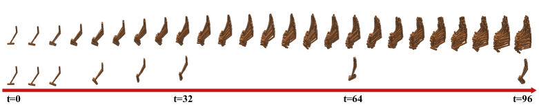
Figure 6: Visual comparison between one-shot generated plans (upper) and PRP (lower) in Hopper. The figure showcases $100$ diffusion-generated plans starting from the same initial state. The one-shot generated plans directly generate all states from $t=0$ to $t=96$, while PRP utilizes three levels with temporal horizons of $97$, $33$, and $9$, and temporal jumps of $32$, $8$, and $1$, respectively. For ease of observation, only Hopper motion every $4$ steps is displayed in the figure.

Table 6: Performance of DiffuserLite under three different temporal horizon choices. All results are obtained over $5$ seeds and the results of default choice are emphasized in bold scores.

Environment	Temporal Horizon - 1
	48	128	256
Hopper-me	$101.1\pm 0.5$	$\bm{111.6\pm 0.2}$	$110.0\pm 0.4$
Hopper-m	$96.6\pm 10.9$	$\bm{100.9\pm 1.1}$	$98.9\pm 0.4$
Hopper-mr	$74.5\pm 27.2$	$\bm{96.6\pm 0.3}$	$98.2\pm 2.1$
Average	$90.7$	$\bm{103.1}$	$102.4$
Kitchen-m	$\bm{73.6\pm 0.7}$	$72.7\pm 1.0$	$25.1\pm 0.2$
Kitchen-p	$\bm{74.4\pm 0.6}$	$75.0\pm 0.0$	$25.2\pm 0.4$
Average	$\bm{74.0}$	$73.9$	$25.2$

Algorithm 2 DiffuserLite Inference

  Input: number of planning levels $L$, temporal horizon $H_{l}$, temporal jump $I_{l}$ and noise estimators $\bm{\epsilon}_{\theta_{l}}$ for each level $l\in\{0,1,\cdots,L-1\}$, critic $\mathcal{C}$, inverse dynamic $h$, diffusion steps $T$, current state $o_{t}$;

  for $l=0$ to $L-1$ do

     sample $\bm{\epsilon}_{l}\sim\mathcal{N}(\bm{0},\bm{I})$.

     first state of $\bm{\epsilon}_{l}\leftarrow o_{t}$

     if $l>0$ then

        last state of $\bm{\epsilon}_{l}\leftarrow$ last state of $\bm{x}_{0:H_{l-1}:I_{l-1}}$

     end if

     obtain $\bm{x}_{0:H_{l}:I_{l}}$ by solving diffusion ODE with DDIM solver

  end for

  extract $o_{t},o_{t+1}$ from $\bm{x}_{0:H_{L-1}:1}$

  $a_{t}=h(o_{t},o_{t+1})$

References

- Ajay et al. (2023) Ajay, A., Du, Y., Gupta, A., Tenenbaum, J. B., Jaakkola, T. S., and Agrawal, P. Is conditional generative modeling all you need for decision making? In The Eleventh International Conference on Learning Representations, ICLR, 2023.
- Atkinson (1989) Atkinson, K. E. An Introduction to Numerical Analysis. John Wiley & Sons, 1989. URL http://www.worldcat.org/isbn/0471500232.
- Ba et al. (2016) Ba, L. J., Kiros, J. R., and Hinton, G. E. Layer normalization. arXiv preprint 1607.06450, ArXiv, 2016.
- Brockman et al. (2016) Brockman, G., Cheung, V., Pettersson, L., Schneider, J., Schulman, J., Tang, J., and Zaremba, W. Openai gym. In arXiv preprint 1606.01540, ArXiv, 2016.
- Chen et al. (2024) Chen, C., Deng, F., Kawaguchi, K., Gulcehre, C., and Ahn, S. Simple hierarchical planning with diffusion. In arXiv preprint 2401.02644, ArXiv, 2024.
- Chi et al. (2023) Chi, C., Feng, S., Du, Y., Xu, Z., Cousineau, E., Burchfiel, B., and Song, S. Diffusion policy: Visuomotor policy learning via action diffusion. In Proceedings of Robotics: Science and Systems, RSS, 2023.
- Dhariwal & Nichol (2021) Dhariwal, P. and Nichol, A. Q. Diffusion models beat GANs on image synthesis. In Advances in Neural Information Processing Systems, NIPS, 2021.
- Dong et al. (2023) Dong, Z., Yuan, Y., Hao, J., Ni, F., Mu, Y., Zheng, Y., Hu, Y., Lv, T., Fan, C., and Hu, Z. Aligndiff: Aligning diverse human preferences via behavior-customisable diffusion model. In arXiv preprint 2310.02054, ArXiv, 2023.
- Dormand & Prince (1980) Dormand, J. R. and Prince, P. A family of embedded runge-kutta formulae. Journal of Computational and Applied Mathematics, 1980.
- Du et al. (2023) Du, Y., Yang, S., Dai, B., Dai, H., Nachum, O., Tenenbaum, J. B., Schuurmans, D., and Abbeel, P. Learning universal policies via text-guided video generation. In Thirty-seventh Conference on Neural Information Processing Systems, NIPS, 2023.
- Emmons et al. (2022) Emmons, S., Eysenbach, B., Kostrikov, I., and Levine, S. Rvs: What is essential for offline RL via supervised learning? In International Conference on Learning Representations, ICLR, 2022.
- Fu et al. (2020) Fu, J., Kumar, A., Nachum, O., Tucker, G., and Levine, S. D4rl: Datasets for deep data-driven reinforcement learning. In arXiv preprint 2004.07219, ArXiv, 2020.
- Gupta et al. (2020) Gupta, A., Kumar, V., Lynch, C., Levine, S., and Hausman, K. Relay policy learning: Solving long-horizon tasks via imitation and reinforcement learning. In Proceedings of the Conference on Robot Learning, PMLR, 2020.
- Hafner et al. (2019) Hafner, D., Lillicrap, T., Fischer, I., Villegas, R., Ha, D., Lee, H., and Davidson, J. Learning latent dynamics for planning from pixels. In International Conference on Machine Learning, ICML, 2019.
- Hansen et al. (2022) Hansen, N., Wang, X., and Su, H. Temporal difference learning for model predictive control. In International Conference on Machine Learning, ICML, 2022.
- He et al. (2023a) He, H., Bai, C., Xu, K., Yang, Z., Zhang, W., Wang, D., Zhao, B., and Li, X. Diffusion model is an effective planner and data synthesizer for multi-task reinforcement learning. In Thirty-seventh Conference on Neural Information Processing Systems, NIPS, 2023a.
- He et al. (2023b) He, H., Bai, C., Xu, K., Yang, Z., Zhang, W., Wang, D., Zhao, B., and Li, X. Diffusion model is an effective planner and data synthesizer for multi-task reinforcement learning. arXiv preprint arXiv:2305.18459, 2023b.
- He et al. (2023c) He, L., Zhang, L., Tan, J., and Wang, X. Diffcps: Diffusion model based constrained policy search for offline reinforcement learning. In arXiv preprint 2310.05333, ArXiv, 2023c.
- Ho & Salimans (2021) Ho, J. and Salimans, T. Classifier-free diffusion guidance. In NeurIPS 2021 Workshop on Deep Generative Models and Downstream Applications, NIPS, 2021.
- Hong et al. (2023) Hong, M., Kang, M., and Oh, S. Diffused task-agnostic milestone planner. arXiv preprint 2312.03395, ArXiv, 2023.
- Janner et al. (2022) Janner, M., Du, Y., Tenenbaum, J. B., and Levine, S. Planning with diffusion for flexible behavior synthesis. In International Conference on Machine Learning, ICML, 2022.
- Jiang et al. (2023) Jiang, C., Cornman, A., Park, C., Sapp, B., Zhou, Y., Anguelov, D., et al. Motiondiffuser: Controllable multi-agent motion prediction using diffusion. In Proceedings of the IEEE/CVF Conference on Computer Vision and Pattern Recognition, pp. 9644–9653, 2023.
- Kawar et al. (2023) Kawar, B., Zada, S., Lang, O., Tov, O., Chang, H., Dekel, T., Mosseri, I., and Irani, M. Imagic: Text-based real image editing with diffusion models. In Proceedings of the IEEE/CVF Conference on Computer Vision and Pattern Recognition, CVPR, 2023.
- Kingma et al. (2021) Kingma, D. P., Salimans, T., Poole, B., and Ho, J. Variational diffusion models. In Advances in Neural Information Processing Systems, NIPS, 2021.
- Kostrikov et al. (2022) Kostrikov, I., Nair, A., and Levine, S. Offline reinforcement learning with implicit q-learning. In The Tenth International Conference on Learning Representations, ICLR, 2022.
- Kumar et al. (2020) Kumar, A., Zhou, A., Tucker, G., and Levine, S. Conservative q-learning for offline reinforcement learning. In Advances in Neural Information Processing Systems, NIPS, 2020.
- Lee et al. (2023) Lee, K., Kim, S., and Choi, J. Refining diffusion planner for reliable behavior synthesis by automatic detection of infeasible plans. In Advances in Neural Information Processing Systems, NIPS, 2023.
- Li et al. (2023) Li, W., Wang, X., Jin, B., and Zha, H. Hierarchical diffusion for offline decision making. In Proceedings of the 40th International Conference on Machine Learning, ICML, 2023.
- Liang et al. (2023) Liang, Z., Mu, Y., Ding, M., Ni, F., Tomizuka, M., and Luo, P. Adaptdiffuser: Diffusion models as adaptive self-evolving planners. In International Conference on Machine Learning, ICML, 2023.
- Liu et al. (2023a) Liu, H., Chen, Z., Yuan, Y., Mei, X., Liu, X., Mandic, D., Wang, W., and Plumbley, M. D. AudioLDM: Text-to-audio generation with latent diffusion models. In Proceedings of the 40th International Conference on Machine Learning, ICML, 2023a.
- Liu et al. (2023b) Liu, X., Gong, C., and qiang liu. Flow straight and fast: Learning to generate and transfer data with rectified flow. In The Eleventh International Conference on Learning Representations, ICLR, 2023b.
- Loshchilov & Hutter (2019) Loshchilov, I. and Hutter, F. Decoupled weight decay regularization. In 7th International Conference on Learning Representations, ICLR, 2019.
- Lu et al. (2022) Lu, C., Zhou, Y., Bao, F., Chen, J., Li, C., and Zhu, J. DPM-solver: A fast ODE solver for diffusion probabilistic model sampling in around 10 steps. In Advances in Neural Information Processing Systems, NIPS, 2022.
- Lu et al. (2023) Lu, C., Ball, P. J., and Parker-Holder, J. Synthetic experience replay. In Workshop on Reincarnating Reinforcement Learning at ICLR, 2023.
- Misra (2020) Misra, D. Mish: A self regularized non-monotonic activation function. In 31st British Machine Vision Conference, BMVC, 2020.
- Ni et al. (2023) Ni, F., Hao, J., Mu, Y., Yuan, Y., Zheng, Y., Wang, B., and Liang, Z. Metadiffuser: Diffusion model as conditional planner for offline meta-rl. International Conference on Machine Learning, ICML, 2023.
- Nichol & Dhariwal (2021) Nichol, A. Q. and Dhariwal, P. Improved denoising diffusion probabilistic models, 2021.
- Pearce et al. (2023a) Pearce, T., Rashid, T., Kanervisto, A., Bignell, D., Sun, M., Georgescu, R., Macua, S. V., Tan, S. Z., Momennejad, I., Hofmann, K., and Devlin, S. Imitating human behaviour with diffusion models. In The Eleventh International Conference on Learning Representations, ICLR, 2023a.
- Pearce et al. (2023b) Pearce, T., Rashid, T., Kanervisto, A., Bignell, D., Sun, M., Georgescu, R., Macua, S. V., Tan, S. Z., Momennejad, I., Hofmann, K., and Devlin, S. Imitating human behaviour with diffusion models. In The Eleventh International Conference on Learning Representations, ICLR, 2023b.
- Peebles & Xie (2022) Peebles, W. and Xie, S. Scalable diffusion models with transformers. arXiv preprint 2212.09748, ArXiv, 2022.
- Ren et al. (2021) Ren, T., Li, J., Dai, B., Du, S. S., and Sanghavi, S. Nearly horizon-free offline reinforcement learning. Advances in neural information processing systems, 34:15621–15634, 2021.
- Ronneberger et al. (2015) Ronneberger, O., Fischer, P., and Brox, T. U-net: Convolutional networks for biomedical image segmentation. arXiv preprint 1505.04597, ArXiv, 2015.
- Ruiz et al. (2023) Ruiz, N., Li, Y., Jampani, V., Pritch, Y., Rubinstein, M., and Aberman, K. Dreambooth: Fine tuning text-to-image diffusion models for subject-driven generation. In Proceedings of the IEEE/CVF Conference on Computer Vision and Pattern Recognition, CVPR, 2023.
- Song et al. (2021a) Song, J., Meng, C., and Ermon, S. Denoising diffusion implicit models. In 9th International Conference on Learning Representations, ICLR, 2021a.
- Song et al. (2021b) Song, Y., Sohl-Dickstein, J., Kingma, D. P., Kumar, A., Ermon, S., and Poole, B. Score-based generative modeling through stochastic differential equations. In International Conference on Learning Representations, ICLR, 2021b.
- Sutton & Barto (1998) Sutton, R. S. and Barto, A. G. Reinforcement learning: An introduction. IEEE Trans. Neural Networks, 1998.
- Tai et al. (2018) Tai, L., Zhang, J., Liu, M., Boedecker, J., and Burgard, W. A survey of deep network solutions for learning control in robotics: From reinforcement to imitation. In arXiv preprint 1612.07139, ArXiv, 2018.
- Thuruthel et al. (2019) Thuruthel, T. G., Falotico, E., Renda, F., and Laschi, C. Model-based reinforcement learning for closed-loop dynamic control of soft robotic manipulators. IEEE Transactions on Robotics, 2019.
- Wang et al. (2023) Wang, Z., Hunt, J. J., and Zhou, M. Diffusion policies as an expressive policy class for offline reinforcement learning. In The Eleventh International Conference on Learning Representations, ICLR, 2023.
- Yu et al. (2023) Yu, T., Xiao, T., Stone, A., Tompson, J., Brohan, A., Wang, S., Singh, J., Tan, C., M, D., Peralta, J., Ichter, B., Hausman, K., and Xia, F. Scaling robot learning with semantically imagined experience. In Proceedings of Robotics: Science and Systems, RSS, 2023.
- Zhang et al. (2023) Zhang, L., Rao, A., and Agrawala, M. Adding conditional control to text-to-image diffusion models. In Proceedings of the IEEE/CVF International Conference on Computer Vision, ICCV, 2023.
- Zhou et al. (2023) Zhou, S., Du, Y., Zhang, S., Xu, M., Shen, Y., Xiao, W., Yeung, D.-Y., and Gan, C. Adaptive online replanning with diffusion models. In arXiv preprint 2310.09629, ArXiv, 2023.
- Zhu et al. (2023a) Zhu, Z., Liu, M., Mao, L., Kang, B., Xu, M., Yu, Y., Ermon, S., and Zhang, W. Madiff: Offline multi-agent learning with diffusion models. In arXiv preprint 2305.17330, ArXiv, 2023a.
- Zhu et al. (2023b) Zhu, Z., Zhao, H., He, H., Zhong, Y., Zhang, S., Yu, Y., and Zhang, W. Diffusion models for reinforcement learning: A survey. In arXiv preprint 2311.01223, ArXiv, 2023b.