XXX

Experimental genuine quantum nonlocality in the triangle network

Abstract

In the last decade, it was understood that quantum networks involving several independent sources of entanglement which are distributed and measured by several parties allowed for completely novel forms of nonclassical quantum correlations, when entangled measurements are performed. Here, we experimentally obtain quantum correlations in a triangle network structure, and provide solid evidence of its nonlocality. Specifically, we first obtain the elegant distribution proposed in [1] by performing a six-photon experiment. Then, we justify its nonlocality based on machine learning tools to estimate the distance of the experimentally obtained correlation to the local set, and through the violation of a family of conjectured inequalities tailored for the triangle network.

Introduction

Bell theorem proved that quantum theory operational implications are irreconcilable with any Local Hidden Variable (LHV) model, or explanation. More precisely, two distant parties (call them Alice and Bob) measuring an appropriate entangled quantum system can observe fundamentally nonclassical space-like separated correlated events, called nonlocal correlations. Bell’s radical conclusion was later confirmed by a series of experiments [2, 3, 4, 5, 6], finally recognized by the Nobel committee in 2022. This milestone theorem had also a profound impact on our understanding of what quantum correlations are or allow for, both for foundational reasons and concrete applications [7, 8].

More recently, it was understood that beyond the standard Bell scenario in which several parties measure a unique quantum state to establish correlations between them, other more general approaches to nonlocality could be considered. In particular, quantum networks, in which several independent sources are distributed to the parties, were shown to display a new form of nonlocality [9, 10, 11, 12, 13, 14]. More precisely, there exists network nonlocal probability distributions, that are distributions obtained by local measurements on several independent quantum sources which have no explanation in terms of classical network LHV strategies. This manifests even without inputs, in particular in the triangle network of Fig. 1 [15, 16, 17, 18].

The concept of quantum network allowed new developments in quantum foundations such as several generalisation of the Bell theorem to exclude other alternatives to quantum theory, beyond LHV models [19, 21, 20, 22, 23, 24]. It also enabled new key applications to quantum correlations [25, 26], e.g. providing strong arguments in favor of the certifiability (self testing) of all pure quantum states [27], a long standing open question.

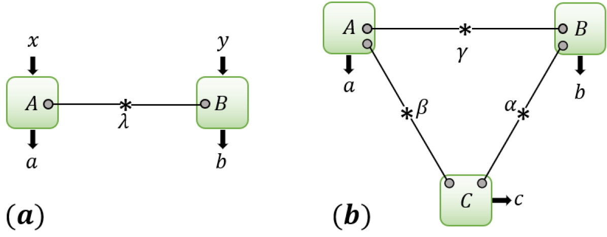
Figure 1: (a) Classical LHV strategy in a standard Bell scenario. The source (star) sample a random variable $\lambda$ and send its value to $A,B$. $A$ outputs $a$, a function of her input $x$ and the value of $\lambda$, $B$ does similarly. With an appropriate bipartite quantum state and local measurements, $A,B$ can obtain correlations with no LHV model explanation.
(b) Classical triangle network LHV strategy . The three sources (star) respectively sample independent random variables $\alpha,\beta,\gamma$ and send their values to $A,B,C$ according to the triangle causal structure. $A$ outputs $a$, a function of the values of $\beta,\gamma$ and $B,C$ do similarly. This allows them to share a probability distribution as in Eq. Network nonlocality in the triangle. In quantum triangle network strategies, the sources produce independent bipartite quantum states, allowing $A,B,C$ to share a probability distribution as in Eq. 2. The EJM distribution of Eq. 4 has a quantum model and is expected to have no classical triangle network LHV strategy explanation.

While well understood algorithms exist to analyse what probability distributions admit a LHV in the standard Bell scenario, characterising correlations in networks is much harder, the problem being not convex. Hence, most analytical proofs of network nonlocality are only valid in the prefect noiseless, infinite statistics case. Some numerical tools exist, such as the inflation method [28], but their numerical complexity make their practical use difficult [29]. More recently, machine learning heuristics were proposed, which construct explicit LHV models, and can find an approximately best LHV model to minimize a given objective function, such as an inequality or the distance to a target distribution [30, 31]. These heuristics are the most efficient approaches to understand whether a generic distribution has a local explanation or not, due to their performance in network scenarios. They have led to conjectures of nonlocality that have since been proven [32]. They are in practice the only tool to study noise robustness of distributions and nonlocality subject to realistic, experimental environments [33].

Very few experimental proofs of quantum network nonlocality where performed. The very first experiments considered the entanglement swapping scenario (or bilocal scenario), which were reported by Saunders et al [34] and Carvacho et al [35] in 2017. In 2019, a more stringent bilocal experiment was performed with several loopholes closed [36]. The experimental studies were also extended to the star networks with up to four branches [37, 38] and the triangle networks [39, 40]. However these experiments are all closely related to standard violation of Bell theorem in a scenario involving a single source and can be realized without entangled measurements. In particular, the last one implements the Fritz distribution [40], which can be viewed as a standard Bell test embedded in the triangle network, in which only one source needs to be entangled and the other two sources can be classically correlated. In the bilocal scenario, several attempt were performed to solve this problem. In particular, the correlations generated by the Elegant Joint Measurements (EJMs) (see Eq. 3 was studied in [1, 41, 42]). A new concept of full network nonlocality was proposed [43] and demonstrated in both bilocal [44] and star networks [45], which certifies all links of the network distribute nonlocal resources. Besides photonic system, Bäumer et al. also demonstrated network nonlocality in a superconducting quantum computer by using deterministic entangled measurements [46]. All these experiments try to obtain genuine network nonlocal correlations, that is nonlocal correlations obtained in a network which cannot be viewed as comming from some embedded standard Bell test in a network [15, 9].

Here, we go beyond the bilocal model and study the correlations generated in the triangle network. Different from previous experimental studies of triangle network, we consider entangled measurements at each node. Specifically, all the three parties are pairwise connected via a polarisation entangled photon source and at each party we perform an EJM. The generated correlation (see Eq. 4) is believed to be genuine to the triangle network, that is not related to standard Bell nonlocality [9]. We use two methods to demonstrate the nonlocality of the observed correlations, both based on a machine-learning-based heuristic program. The first is using the machine learning program to calculate the minimal distance between the observed correlation to the local hidden variable models. The other is observing the violation of a family of inequalities inspired by the machine learning program. Our results demonstrate that experimental observing this new form of nonlocality is possible with current technology.

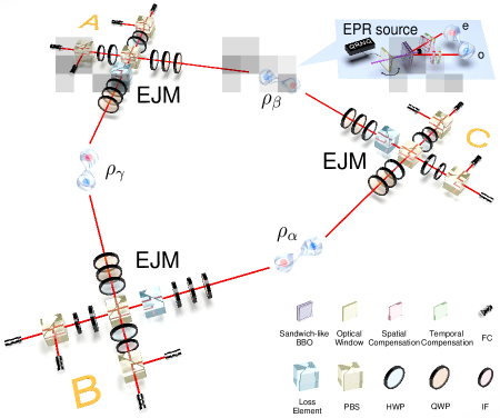
Figure 2: Sketch of the experimental setup. Three EPR sources distribute biphoton singlet state through a spontaneous parametric downconversion process. The EPR source is a sandwich-like BBO-HWP-BBO structure with 390-nm, 80-MHz, 140-fs ultraviolet pulse pumping. An optical window controlled by the QRNG randomizes the phase of the pump pulse before it is incident on the crystal. Each node of the network receives an ordinary photon (red sphere) and an extraordinary photon (blue sphere), which come from two different sources. At each node, the partially entangled projection is achieved through the polarization-dependent loss element and photonic Hong-Ou-Mandel interference, and the ideal EJM is simulated by switching the projection settings. FC fiber coupler, PBS polarization beam splitter, HWP half-wave plate, IF interference filter, QRNG quantum random number generator, BBO beta barium borate.

Results

Network nonlocality in the triangle

In the triangle network, with classical bipartite sources, the three parties are able to sample from probability distributions of the form

$$P(a,b,c)= \int d\alpha d\beta d\gamma P_{\alpha}(\alpha)P_{\beta}(\beta)P_{\gamma}(\gamma)$$

$$P_{A}(a|\beta,\gamma)P_{B}(b|\gamma,\alpha)P_{C}(c|\alpha,\beta),$$ (1)

where $P_{A}(a|\beta\gamma)$ denoted the response function of Alice given some values of the local hidden varaibles $\beta$ and $\gamma$ that she has access to, and similarly for Bob and Charlie, and with a slight abuse of notation $P_{\alpha}(\alpha)$ denotes the probability of $\alpha$ for source $\alpha$ and similarly for $\beta$, $\gamma$. Note that we are currently interested in the discrete outcome case, in particular where $a,b,c\in\{1,2,3,4\}$.

In contrast to the classical correlations, having access to bipartite quantum sources allows one to sample from distributions of the form

$$P(a,b,c)=\text{Tr}\left(\rho_{\alpha}\rho_{\beta}\rho_{\gamma}M_{A}^{a}M_{B}^{b}M_{C}^{c}\right),$$ (2)

where $\rho_{\alpha}$ is the density matrix of the quantum state distributed by source $\alpha$ and similarly for $\beta,\gamma$, and $\{M_{A}^{a}\}_{a}$ is a Positive Operator-Valued Measure such that $M_{A}^{a}\geq 0$ and $\sum_{a}M_{A}^{a}=\mathbb{I}$, and similarly for Bob and Charlie. Note that for example the source $\alpha$ distributes one part of its state to Bob and one to Charlie, so it is important to take into account the Hilbert space structure, i.e. one could write $\rho_{\alpha}\equiv\rho_{B2,C1}$ and $M_{B}^{b}=M_{B1,B2}^{b}$, etc., in order to account for the proper subspaces.

When a distribution $P$ has no classical explanation according Eq. Network nonlocality in the triangle, it is called triangle-nonlocal, or simply just nonlocal in the current context. Currently few distributions have been proven to be nonlocal in the triangle network, and several conjectures for nonlocality exist which have not been proven, yet have numeric evidence supporting it. Among these we focus on the Elegant distribution, introduced in Ref. [1], with supporting numeric and analytic studies for its nonlocality in Refs. [30, 31, 47]. To sample from the distribution the source should distribute singlets, and the parties should measure in the basis

$$\ket{\Phi_{i}}=\frac{\sqrt{3}+1}{2\sqrt{2}}\ket{\vec{m}_{i},-\vec{m}_{i}}+\frac{\sqrt{3}-1}{2\sqrt{2}}\ket{-\vec{m}_{i},\vec{m}_{i}},$$ (3)

where $i\in\{1,2,3,4\}$, $\vec{m_{i}}$ are vertices of a tetrahedron in the Bloch sphere, $\ket{\vec{m}_{i}}$ are the corresponding single qubit states, and $\langle\vec{m}_{i}|-\vec{m}_{i}\rangle=0$. The distribution obtained from these so-called EJMs is symmetric both under permutation of the parties and of the outcomes, and can thus be characterized by 3 parameters (or 2 when considering normaliztion),

$$P_{E}(a,b,c)=\begin{cases}\frac{25}{256}&a=b=c,\\ \frac{1}{256}&a=b\neq c\text{ or }b=c\neq a\text{ or }c=a\neq b,\\ \frac{5}{256}&a\neq b\neq c\neq a.\end{cases}$$ (4)

Though the nonlocality of this distribution is not yet proven, there is surmounting evidence that it is nonlocal, and in fact has a strong noise robustness with respect to specific noise models. Moreover, this distribution violates a recently conjectured Bell-type inequality, i.e. one that is conjectured to be satisfied by all LHV models. The inequality is robust and interpretable, capturing the fact that classical strategies can not be as strongly correlated in $(k,k,k)$-type outcomes as quantum distributions can, while maintaining symmetry [31].

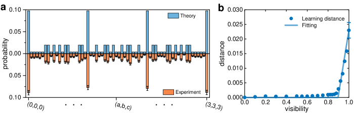
Figure 3: Experimental result. a The theoretical and experimental elegant distribution. The experimental distribution is obtained by normalizing the raw experimental data in all projection settings. b The effect of measurement visibility on the distance from the experimental distribution to the local set. There is a critical visibility, below which the distance approaches 0 and is almost constant, and above which the distance increases almost linearly with visibility. The error bars are deduced from the photon statistical error.

Optical triangle network

The triangle network is constructed from three optical Einstein-Podolsky-Rosen (EPR) sources, each of which is located on one of the three sides of the triangle. The source generates photon pairs through spontaneous parametric downconversion (SPDC) process, in a “sandwich-like” nonlinear crystals pumped by an ultrafast laser pulse. The EPR source generates polarization-entangled state $\ket{\psi^{-}}=(\ket{HV}-\ket{VH})/\sqrt{2}$, and the qubits are encoded in the polarization degree of freedom of the photons. Each node of the triangle network receives two photons from two different EPR sources. The experimental sketch is shown in Fig. 2.

An important condition is that the EPR sources should be independent of each other. To improve the independence of the sources, we split the pulse from the single laser into three and let them pump the three EPR sources in parallel so that the photon pairs are generated from independent crystals. Then we insert a tiltable optical window in each pumping path. The tilt angle of the optical windows, which can change the optical distance, are controlled by independent quantum random number generators. In this way, the randomly tilted window imposes a completely random phase for each pump beam, thus erasing the coherent information between them. Such a method has been used in previous studies of network nonlocality [34, 45].

The three nodes of the network all perform fixed EJM, thus there are no external inputs. The implementation of the ideal EJM requires two cascaded control operations [41]. Just like the common Bell state measurement, it is impossible to implement deterministic entangling operations with only linear optics. However, we can simulate the ideal EJM outputs statistically by projecting the input state onto each of the four EJM bases separately. Specifically, we construct four projection settings in the experiment, each corresponding to one of the EJM bases, switch these settings randomly during the experiment and finally combine the results obtained from these settings, as a result the statistical distribution obtained is the same as the ideal EJM. As shown in Eq. 3, the EJM bases are both partially entangled and have the same Schmidt coefficients. Our EJM basis projection device contains two parts. One is a partially entangled projection device that projects the input state into a partially entangled state with the same Schmidt coefficient as the EJM bases. This consists of a standard photonic polarization Bell state projection setup, and a customized polarization-dependent loss element that biases the Schmidt coefficients of the projected state to match the EJM bases. Another one is a basis transformer that enables the transformation between $\ket{H}/\ket{V}$ and the Schmidt bases $\ket{\vec{m}_{i}}/\ket{-\vec{m}_{i}}$ of EJM bases. This is achieved by three cascade wave plates mounted on motorized rotation stages. Switching between the four projection settings is accomplished only by rotating the cascade wave plates to the corresponding angles. (See more details in Methods.) Each node simulates the ideal EJM in this way, eventually normalizing the raw data we can obtain the elegant distribution.

Experimental results

We first characterize the experimental setup. Our EPR sources achieve both high brightness (0.2 MHz) and high collection efficiency (31%), and with quantum state tomography we find its fidelity (defined as $F=\bra{\psi^{-}}\rho\ket{\psi^{-}}$) to be $0.9769\pm 0.0001$, $0.9761\pm 0.0001$, and $0.9802\pm 0.0001$, respectively. Similarly, we analyze the measurement setup at each node with measurement tomography, obtaining a fidelity of $0.9352\pm 0.0017$, $0.9384\pm 0.0020$, and $0.9382\pm 0.0019$, respectively.

During the experiment, we perform 64 measurement settings (each node has 4 settings) to obtain an elegant distribution. To reduce the impact of laser power fluctuations on counting rates, we randomly switch the measurement settings every 10 minutes. Each setting is measured 27 times, and finally, we collect 3343 six-fold events in 288 hours. The optical windows randomly switch tilt angles every 20 milliseconds, which is much less than the time required to detect a six-fold event; thus, we can say that the quantum coherence between the three pump beams is destroyed on the time scale of the network. We plot the experimental elegant distribution $P_{\text{Exp}}$ against the theoretical distribution in Fig. 3(a).

To determine whether our experimental elegant distribution $P_{\text{Exp}}$ is compatible with a local model, we first input it to the neural network oracle. If $P_{\text{Exp}}$ is inside the local set, then the neural network returns the local model that reproduces $P_{\text{Exp}}$. If $P_{\text{Exp}}$ is outside the local set, then the neural network returns the local distribution $P_{\text{NN}}$ closest to it. The closest means the Euclidean distance between $P_{\text{NN}}$ and $P_{\text{Exp}}$, which is defined as $\sqrt{\sum_{a,b,c}^{3}\big{[}P_{\text{Exp}}(a,b,c)-P_{\text{NN}}(a,b,c)\big{]}^{2}}$, is minimal. By independently running the neural network 60 times, we find that the minimal distance of the local set from $P_{\text{Exp}}$ is $0.0230\pm 0.0027$, where the uncertainty is determined by running 50 Monte Carlo simulations of the measured data based on Poisson distributed photon statistics and calculating the minimal distance of each set of the simulated data by using the neural network. The uncertainty represents one standard deviation and contains both the photonic statistical error and the error induced by the neural network. To show that the experimental distribution is indeed outside the local set, we analyze how the measurement visibility (see Methods for more details) affects the distance to the local set. As the visibility continues to decrease, we expect the distance to decrease until it drops to 0 after some critical point, below which the noise distribution can be reproduced by the local model. Due to the limited numerical precision of the neural network and its training, it is not possible for it to return a local model that exactly replicates the noise distribution, so the distance will not be exactly 0 but rather a very small value. As shown in Fig. 3(b),we fit the points with visibility from 0.9 to 1 into a line. The line intersects the x-coordinate at about 0.89 which we treat as the critical visibility. Our experimental elegant distribution $P_{\text{Exp}}$, which corresponds to the point with visibility equal to 1, has a distance to the local set that is more than 8 standard deviations larger than the distance at the critical point, which predicts that $P_{\text{Exp}}$ is indeed outside the local set and exhibits high robustness.

In Ref. [31], the authors conjecture two families of inequalities, each depending on a parameter $w$, which captures the trade-off between the strong correlations and the strictness of the symmetry constraint. Our experimental distribution violates the one using a squared asymmetry penalty. In the original work, they identify $w\approx 0.16$ as the optimal $w$ value, when considering the theoretical distribution $P_{E}$. Though we violate the inequality for this value as well, we find that for other $w$ values the violation is much stronger (see Methods, Fig. 4). In particular at $w\approx 0.0922$ we achieve a violation of $0.00400\pm 0.00077$, which is 42% of the value that the theoretic elegant distribution achieves ($0.00957$), for the inequality

$$0.0922\,s_{111}(P)-0.9078\,\Delta(P)\leq 0.0264,$$ (5)

where

$$s_{111}(P)=P(a=b=c)=\sum_{k}P(k,k,k)$$ (6)

captures the strength of the correlations, while $\Delta$ gives a penalty for being non-symmetric by summing up the deviations from the mean of each of the 3 types of events ((1,1,1); (1,1,2); and (1,2,3) -type outcomes), via

$$\Delta(P)= \sum_{X\in\{111,112,123\}}\sum_{\{a,b,c\}\in\mathcal{I}_{X}}|M_{X}-P(a,b,c)|^{2},$$ (7)

$$M_{X}= \frac{1}{|\mathcal{I}_{X}|}\sum_{\{a,b,c\}\in\mathcal{I}_{X}}P(a,b,c),$$ (8)

where $\mathcal{I}_{X}$ is the index set of $X$-type outcomes (in particular $\mathcal{I}_{111}$ will contain 4 elements, $\mathcal{I}_{112}$ 36, and $\mathcal{I}_{123}$ 24 elements). For our experimental distribution, $s_{111}(P_{\text{Exp.}})\approx 0.334,\,\Delta(P_{\text{Exp.}})\approx 0.000409$, whereas for the theoretical distribution $s_{111}(P_{\text{E}})=\frac{100}{256}\approx 0.3906,\,\Delta(P_{\text{E}})=0$.

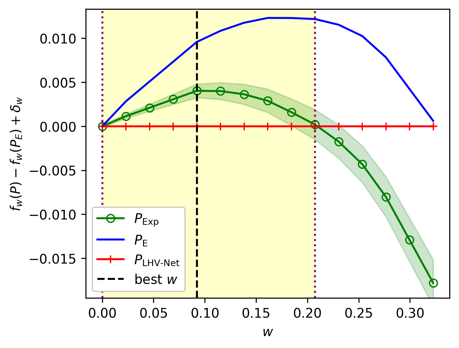
Figure 4: Violations of the conjectured inequality as a function of $w$, for the ideal EJM distribution (blue), the experimental results (green), and for classical strategies found by LHV-Net (red). Green band denotes one standard deviation, and yellow area displays $w$ values for which the inequality is violated by the experimental data. The strongest violation is observed at $w\approx 0.09$, reaching about 42% of the ideal distribution’s violation.

Discussion

Quantum nonlocality plays an important role in quantum physics foundations and for quantum information technologies. Moving beyond the standard Bell scenario, it was proven that the correlations generated in quantum networks which consist of independent entangled sources and entangled measurements can exhibit new forms of nonlocality, in some cases even no external inputs are required. Here, we experimentally study the elegant distribution generated in the triangle network, a striking example of network nonlocality which is genuine to networks, that is cannot be interpreted as coming from standard Bell nonlocality. We provide strong evidences that our experimentally observed distribution can not be explained with a LHV triangle network local model.

Note however that our experiment is subject to the common loopholes in the standard Bell experiments, namely the locality loophole and the fair sampling loophole. In addition, the network local model also opens a new source independence loophole. More precisely, in the triangle network, the three distributed quantum sources should be independent. However, just like the freedom of choice loophole in the standard Bell test, no argument can prove that this independence fully holds. This condition can only be made more stringent, but the associated independence loophole, explaining the obtained correlations through correlated sources (which can then be distributing a LHV model) can never be closed. In this work, we experiemntaly enhance the source independence by erasing the coherence information between the pump beams of the sources, similarly to what has been used in several previous studies.

Contrary to previous experiements of triangle network nonlocality implementing the Fritz distribution [40], the elegant distribution generated in our experiment is thought to be genuine to the triangle network, in the sense that it cannot be interpreted as reproducing a standard forms of Bell nonlocality embedded in the triangle scenario. In particular it relies on the use of entangled measurements at each party, while the Fritz’s model can be realized by only separable measurements.

Another feature that differentiates the elegant model to the standard Bell scenario is that the elegant distribution can be generated by fixed measurements without external inputs. Although in the experiment we didn’t achieve an ideal EJM, we only simulate the statistics of an ideal one by projecting onto each elegant basis separately, the distribution can be obtained in principle simultaneously. This is different from the situation in the standard Bell test, in which at least two non-commute observers need to be measured at each party to generate the nonlocal correlations. Note that this unideal realization may introduce the freedom of choice loophole like the standard Bell test. This loophole might closed in the future experiment with deterministic photon-photon gates, for example, by using cavity-QED system.

Methods

Neural network search for local hidden variable models

Since an analytic proof is not available for the nonlocality of the Elegant distribution, we use the best available numeric methods to reinforce that our experimental results could not have been obtained from a classical model according to Eq. Network nonlocality in the triangle. Specifically, we use the neural network-based ansatz developed in Ref. [30], (LHV-Net). In this, the authors show that modeling local hidden variable models with artificial neural networks is a reliable heuristic, reproducing benchmark results, as well as providing new conjectures, which have since been partially proven [32].

A feed-forward artificial neural network is a numeric model for any multivariate, multidimensional function. Its parameters can be fit (it can be trained), in order to minimize a differentiable objective function. The core idea of LHV-Net is to model each of the response functions in (Network nonlocality in the triangle) with neural networks. For example Alice’s neural network would take as inputs some $\beta_{i}$, $\gamma_{i}$, and output a normalized vector $P_{A}^{\text{NN}}(a|\beta_{i},\gamma_{i})\in\mathbb{R}^{4}$. Sampling over many ($M$) triples $(\alpha_{i},\beta_{i},\gamma_{i})\in[0,1]^{3}$, one arrives at a Monte Carlo estimate of (Network nonlocality in the triangle),

$$P_{\text{NN}}=\frac{1}{M}\sum_{i=1}^{M}P_{A}^{\text{NN}}(a|\beta_{i},\gamma_{i})P_{B}^{\text{NN}}(b|\gamma_{i},\alpha_{i})P_{C}^{\text{NN}}(c|\alpha_{i},\beta_{i}).$$ (9)

Importantly, each party’s neural network only has access to the respective hidden variables allowed by the triangle structure, thus any distribution given by LHV-Net is by construction local.

In order to train the neural network we first use the objective function $||P_{\text{Exp}}-P_{\text{NN}}||^{2}$, where $P_{\text{Exp}}$ is the experimentally obtained distribution. If the distribution could be explained by a classical (local hidden variable) model, we expect the neural network would find it and the resulting objective would reach zero. As portrayed in the Results section, the closest local model the neural network could find is $0.0230\pm 0.0027$, well above the zero value. In contrast, in Ref. [30], the authors find a distance of approximately $0.05$ for the $P_{E}$, the theoretical Elegant distribution. The fact that our experimental results are at about $50\%$ distance between the noiseless Elegant distribution and the local set gives us great confidence that such results could not have been obtained using a classical triangle network.

Finally, note that LHV-Net, together with analytic considerations, has been used to derive the inequalities stated in the Results section, by changing the objective function from a distance function to an inequality [31]. In detail, one can define the function

$$f_{w}(p)=w\cdot s_{111}(P)-(1-w)\Delta(P),$$ (10)

with $s_{111}(P)$ and $\Delta(P)$ defined in (6) and (7), respectively. Then one compares the maximum that this function takes over LHV models, and compares it to the value that $P_{E}$ achieves,

$$\delta_{w}:=f_{w}(P_{E})-\max_{P\in\mathcal{L}}f_{w}(P),$$ (11)

where $\mathcal{L}$ is the set of distributions admitting an LHV model. If $\delta_{w}>0$, then the inequality for that $w$ is a Bell inequality which certifies the nonlocality of $P_{E}$,

$$f_{w}(P)\leq f_{w}(P_{E})-\delta_{w}.$$ (12)

Using the numeric tools of LHV-Net, one can obtain an estimate of the $\delta_{w}$ values, as was done in Ref. [31]. In Fig. 4 we plot $f_{w}(P)-f_{w}(P_{E})+\delta_{w}$, which should be negative or 0 for all local distributions. From the results we deduce that the inequality which most strongly certifies our experimental distribution is for $w\approx 0.0922,\,\delta_{w}\approx 0.00957$, resulting in the inequality of Eq. (5). We identified this $w$ value by finding the largest ratio between the violation of $P_{\text{Exp.}}$ and $P_{E}$, which was 42%.

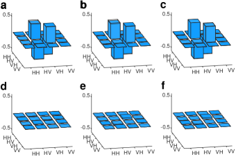
Figure 5: Tomographic results of the three EPR sources. a, b, and c are the real parts of $S_{\alpha}$, $S_{\beta}$, and $S_{\gamma}$ respectively. d, e, and f are the imaginary parts of $S_{\alpha}$, $S_{\beta}$, and $S_{\gamma}$ respectively.

EPR source

The production of entangled photons is based on the spontaneous parametric downconversion (SPDC) process pumped by ultraviolet pulses. The pump pulses with a central wavelength of 390 nm are obtained from the frequency doubling system, where the fundamental frequency laser pulses are generated by the mode-locked Ti:sapphire laser with a center wavelength of 780 nm, a duration of 140 fs, and a repetition rate of 80 MHz. The EPR source is a sandwich-like structure composed of a true-zero-order half-wave plate (THWP) between two beta barium borate (BBO) crystals. Both BBO crystals are 2 mm thick and are identically cut for beam-like Type-II phase matching. When the ultraviolet laser pulse is incident on the crystal, both BBO crystals probabilistically produce a pair of extraordinary (e) and ordinary (o) photons with horizontal and vertical polarizations, i.e., $\ket{HV}$. The photons generated by the first BBO, however, will have their polarization flipped by the middle THWP, resulting in a state $\ket{VH}$. Then after temporal and spatial compensation, the two SPDC processes become indistinguishable, and the two-photon state becomes a singlet $\ket{\psi^{-}}=(\ket{HV}-\ket{VH})/\sqrt{2}$.

In the experiment, we construct three EPR sources, each pumped with 340 mW ultraviolet pulses. When using a 3 nm spectrum filter for each side of the collection, each source has a counting rate of approximately 0.2 MHz, and the collection efficiency is approximately $31\%$. To characterize these EPR sources, we perform state tomography for each of them. The reconstructed density matrices are shown in Fig. 5, and the fidelity of the state $F=\bra{\psi^{-}}\rho\ket{\psi^{-}}$ is calculated to be $0.9769\pm 0.0001$, $0.9761\pm 0.0001$, and $0.9802\pm 0.0001$, respectively.

Source independence

The three sources are each pumped by three parallel pulses split from a single pulse. In each of the pumping paths, we insert a tiltable optical window, a 5 mm thick N-BK7 glass slice mounted on a motorized rotation stage, to impose an additional phase to the pulse. When the optical window deviates from the normal incidence angle by $0.6^{o}$, the pulse will have an additional optical distance of approximately 410 nm. During the experiment, three different quantum random number generators (QRNGs) control the tilt angle of the three optical windows. Each QRNG generates random numbers between 0 and 1, which are then mapped to angles with a resolution of $0.01^{o}$ between $0^{o}$ and $0.6^{o}$ to tilt the optical window, thereby applying random phase shifts between 0 and $2\pi$ to the pump beam. This process is repeated approximately every 20 ms, which is much faster than our six-fold counting rate of approximately $12$ per hour. Thus, the relative phase information of the three pump beams is effectively erased.

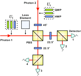
Figure 6: EJM basis projection device. The transmittance of the loss element to horizontal polarized photon is $T_{H}=1$, while to vertical polarized photon is $T_{V}=7-4\sqrt{3}$. Each detector is preceded by an interference filter not shown.

Elegant joint measurement

The EJM basis projection device is shown in Fig. 6. There is a standard Bell state projector consisting of a polarization beam splitter (PBS) with a $45^{o}$ half-wave plate (HWP) on the photon 2 path and two $22.5^{o}$ HWPs at each output of the PBS, the input state will be projected onto $(\ket{HV}+\ket{VH})/\sqrt{2}$ when the two output photons are located in the paths of detectors 1 and 3 or 2 and 4 respectively. The transformation made by the $45^{o}$ HWP can be absorbed into the unitary transformation. To match the Schmidt coefficients of the EJM bases, which are biased, we insert a polarization-dependent loss element in the path of photon 1 that is fully transmissive to $\ket{H}$ photon but has a transmittance of $7-4\sqrt{3}$ to $\ket{V}$ photon. By attenuating some of the vertical-polarized photons, the input state is projected toward a partially entangled state $\sqrt{\eta}(\frac{\sqrt{3}+1}{2\sqrt{2}}\ket{HV}+\frac{\sqrt{3}-1}{2\sqrt{2}}\ket{VH})$. Due to the introduction of the loss element, the projection efficiency becomes $\eta=2(2-\sqrt{3})$. The two quarter-wave plates (QWPs) and one HWP at each input act as a basis transformer, which performs the unitary $U_{i}$ for each photon where $U_{i}\ket{\vec{m_{i}}}=\ket{H}$ and $U_{i}\ket{-\vec{m_{i}}}=\ket{V}$, so that the $\ket{H}/\ket{V}$ bases of the Bell state projector and the Schmidt bases $\ket{\vec{m}_{i}}/\ket{-\vec{m}_{i}}$ of the EJM basis can be converted. These wave plates are mounted on motorized rotation stages and can be rotated to specific angles to realize the conversion of any four sets of Schmidt bases of the EJM. Overall, the setup can project the input state toward any of the EJM bases $\sqrt{\eta}(\frac{\sqrt{3}+1}{2\sqrt{2}}\ket{\vec{m}_{i},-\vec{m}_{i}}+\frac{\sqrt{3}-1}{2\sqrt{2}}\ket{-\vec{m}_{i},\vec{m}_{i}})$, $i=1,2,3,4$. Note that the projection efficiency is the same for each projection setting, and the experimental results do not need to be renormalized for efficiency.

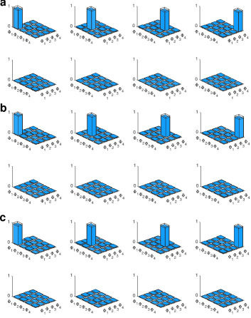
Figure 7: Tomographic results of EJM on three nodes. a, b, and c contain the reconstructed POVM elements on nodes A,B, and C, respectively, which are shown in EJM bases $\{\Phi_{1},\Phi_{2},\Phi_{3},\Phi_{4}\}$. In each subfigure, the top four are the real parts of the reconstruction matrices and the bottom four are the corresponding imaginary parts.

By means of the measurement tomography, we obtain the reconstructed matrices of the measurements at the three nodes with fidelity of $0.9352\pm 0.0017$, $0.9384\pm 0.0020$, and $0.9382\pm 0.0019$. The results are shown in Fig. 7. Since the measurement setup is mainly affected by white noise, the original projectors became a series of Positive Operator-Valued Measure (POVM) elements in the experiment.

Measurement visibility

The measurement visibility is determined by the intensity of white noise. Considering that our experimental measurement process suffers from more white noise, that is the POVM elements at nodes $A$, $B$ and $C$ become $\nu E^{A}_{i}+\frac{1-\nu}{4}I^{A}$, $\nu E^{B}_{j}+\frac{1-\nu}{4}I^{B}$, and $\nu E^{C}_{k}+\frac{1-\nu}{4}I^{C}$, where $i,j,k\in\{0,1,2,3\}$ depend on the measurement output, and $\sum_{i=0}^{3}E^{A}_{i}=I^{A}$, $\sum_{j=0}^{3}E^{B}_{j}=I^{B}$, $\sum_{k=0}^{3}E^{C}_{k}=I^{C}$. The measurement visibility $\nu$ is between 0 and 1, $\nu=1$ denotes our experimental measurement process, and $\nu=0$ indicates that the measurement output is completely random. Based on this, we can calculate the noise distribution $P_{\nu}(i,j,k)$ at arbitrary measurement visibility using the following equation:

$$\centering P_{\nu}(i,j,k)\@add@centering =\mathrm{Tr}\big{[}\rho(\nu E^{A}_{i}+\frac{1-\nu}{4}I^{A})(\nu E^{B}_{j}+\frac{1-\nu}{4}I^{B})(\nu E^{C}_{k}+\frac{1-\nu}{4}I^{C})\big{]}$$

$$=\nu^{3}\mathrm{Tr}\big{[}\rho E^{A}_{i}E^{B}_{j}E^{C}_{k}\big{]}+\nu^{2}\frac{1-\nu}{4}(\mathrm{Tr}\big{[}\rho E^{A}_{i}E^{B}_{j}I^{C})\big{]}+\mathrm{Tr}\big{[}\rho E^{A}_{i}I^{B}E^{C}_{k})\big{]}+\mathrm{Tr}\big{[}\rho I^{A}E^{B}_{j}E^{C}_{k})\big{]})$$

$$\quad\ +\nu(\frac{1-\nu}{4})^{2}(\mathrm{Tr}\big{[}\rho E^{A}_{i}I^{B}I^{C})\big{]}+\mathrm{Tr}\big{[}\rho I^{A}E^{B}_{j}I^{C})\big{]}+\mathrm{Tr}\big{[}\rho I^{A}I^{B}E^{C}_{k})\big{]})+(\frac{1-\nu}{4})^{3}\mathrm{Tr}\big{[}\rho I^{A}I^{B}I^{C})\big{]}$$

$$=\nu^{3}P_{\text{Exp}}(i,j,k)+\nu^{2}\frac{1-\nu}{4}(\sum_{k^{\prime}=0}^{3}P_{\text{Exp}}(i,j,k^{\prime})+\sum_{j^{\prime}=0}^{3}P_{\text{Exp}}(i,j^{\prime},k)+\sum_{i^{\prime}=0}^{3}P_{\text{Exp}}(i^{\prime},j,k))$$

$$\quad\ +\nu(\frac{1-\nu}{4})^{2}(\sum_{j^{\prime},k^{\prime}=0}^{3}P_{\text{Exp}}(i,j^{\prime},k^{\prime})+\sum_{i^{\prime},k^{\prime}=0}^{3}P_{\text{Exp}}(i^{\prime},j,k^{\prime})+\sum_{i^{\prime},j^{\prime}=0}^{3}P_{\text{Exp}}(i^{\prime},j^{\prime},k))+(\frac{1-\nu}{4})^{3}$$ (13)

where $P_{\text{Exp}}$ is the experimental elegant distribution. Feeding it into a neural network, we can learn how the measurement visibility $\nu$ affects the distance from the distribution to the local set.

Supplementary materials

Experimental details

Fig. 8 shows the raw data of the six-fold coincidence events for the 64 measurement settings. Each output c of node C corresponds to a panel. The vertical axis of each panel corresponds to the output a of node A and the horizontal axis corresponds to the output b of node B. By normalizing the 64 raw data, we can get the experimental elegant distribution $P_{\text{Exp}}(a,b,c)$.

Fig. 9 shows the detailed experimental setup, which consists of four parts from top to bottom: the preparation and distribution of the ultraviolet pulses, the EPR sources, the fiber distribution, and the measurement processes. The ultrafast laser pulses generated by the mode-locked Ti:sapphire laser (with a central wavelength of 780 nm, a pulse duration of 140 fs, and a repetition rate of 80 MHz) are first passed through a frequency doubler. The output ultraviolet laser is split into three beams averagely by using a series of HWPs and PBSs, The relative phases between the beams are erased by inserting randomly rotated optical windows before they hit on the sandwich-like BBO crystals. Then the produced downcoversion photons are distributed to the three nodes by optical fibers, each of which receives one ordinary photon and one extraordinary photon from two different sources. In the measurement device, both photons pass through three cascaded wave plates, the extraodinary photon also passes through a polarization-dependent loss element. Then the two photons are overlapped on the central PBS for HOM interference. Then the two photons are measured in $|\pm\rangle$ basis, where $|\pm\rangle=(|0\rangle\pm|1\rangle)/\sqrt{2}$. When both output ports detect one photon and have the same polarization, the projection device succeeds. When all three projection devices succeed, we record a six-fold coincidence event.

Figure 8: Six-fold coincidence counts corresponding to different measurement outputs.

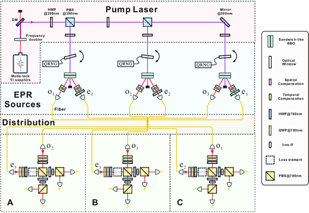
Figure 9: The detailed experimental setup.

References

- [1] Gisin, N. Entanglement 25 Years after Quantum Teleportation: Testing Joint Measurements in Quantum Networks. Entropy 21, 325 (2019).
- [2] Freedman, S. J. & Clauser, J. F. Experimental Test of Local Hidden-Variable Theories. Phys. Rev. Lett. 28, 938 (1972).
- [3] Aspect, A., Grangier, P. & Roger, G. Experimental Realization of Einstein-Podolsky-Rosen-Bohm Gedankenexperiment: A New Violation of Bell’s Inequalities. Phys. Rev. Lett. 49, 91 (1982).
- [4] Hensen, B. et al. Loophole-free Bell inequality violation using electron spins separated by 1.3 kilometres. Nature 526, 682 (2015).
- [5] Giustina, M. et al. Significant-Loophole-Free Test of Bell’s Theorem with Entangled Photons. Phys. Rev. Lett. 115, 250401 (2015).
- [6] Shalm, L. K. et al. Strong Loophole-Free Test of Local Realism. Phys. Rev. Lett. 115, 250402 (2015).
- [7] Barrett, J., Hardy, L. H. & Kent, A. No Signaling and Quantum Key Distribution. Phys. Rev. Lett. 95, 010503 (2005).
- [8] Pironio, S. et al. Random numbers certified by Bell’s theorem. Nature 464, 1021 (2010).
- [9] Tavakoli, A., Pozas-Kerstjens, A., Luo, M.-X. & Renou, M.-O. Bell nonlocality in networks. Rep. Prog. Phys. 85, 056001 (2022).
- [10] Branciard, C., Gisin, N. & Pironio, S. Characterizing the Nonlocal Correlations Created via Entanglement Swapping. Phys. Rev. Lett. 104, 170401 (2010).
- [11] Branciard, C. et al. Bilocal versus nonbilocal correlations in entanglement-swapping experiments. Phys. Rev. A 85, 032119 (2012).
- [12] Tavakoli, A. et al. Nonlocal correlations in the star-network configuration. Phys. Rev. A 90, 062109 (2014).
- [13] Chaves, R. Polynomial Bell Inequalities. Phys. Rev. Lett. 116, 010402 (2016).
- [14] Rosset, D. et al. Nonlinear Bell Inequalities Tailored for Quantum Networks. Phys. Rev. Lett. 116, 010403 (2016).
- [15] Renou, M.-O. et al. Genuine Quantum Nonlocality in the Triangle Network. Phys. Rev. Lett. 123, 140401 (2019).
- [16] M.-O. Renou, S. Beigi Nonlocality for Generic Networks Phys. Rev. Lett. 128, 060401 (2022)
- [17] M.-O. Renou, S. Beigi Network Nonlocality via Rigidity of Token-Counting and Color-Matching Phys. Rev. A 105, 022408 (2022)
- [18] Alejandro Pozas-Kerstjens, Nicolas Gisin, Marc-Olivier Renou Proofs of network quantum nonlocality in continuous families of distributions Phys. Rev. Lett. 130, 090201 (2023)
- [19] M. Weilenmann, R. Colbeck Self-Testing of Physical Theories, or, Is Quantum Theory Optimal with Respect to Some Information-Processing Task? Phys. Rev. Lett. 125, 060406 (2020)
- [20] Renou, M.-O. et al. Quantum theory based on real numbers can be experimentally falsified. Nature 600, 625 (2021).
- [21] Li, Z.-D. et al. Testing real quantum theory in an optical quantum network . Phys. Rev. Lett. 128, 040402 (2022).
- [22] Coiteux-Roy, X., Wolfe, E. & Renou, M.-O. No Bipartite-Nonlocal Causal Theory Can Explain Nature’s Correlations. Phys. Rev. Lett. 127, 200401 (2021).
- [23] Coiteux-Roy, X., Wolfe, E. & Renou, M.-O. Any physical theory of nature must be soundlessly multipartite nonlocal. Phys. Rev. A 104, 052207 (2021).
- [24] Cao, H et al. Experimental Demonstration that No Tripartite-Nonlocal Causal Theory Explains Nature’s Correlations Phys. Rev. Lett. 129, 150402 (2022)
- [25] M.-O. Renou, J. Kaniewski, N. Brunner Self-Testing Entangled Measurements in Quantum Networks Phys. Rev. Lett. 121, 250507 (2018)
- [26] Sekatski, P., Boreiri, S. & Brunner, N. Partial Self-Testing and Randomness Certification in the Triangle Network. Phys. Rev. Lett. 131, 100201 (2023).
- [27] Šupić, I. et al. Quantum networks self-test all entangled states. Nat. Phys. 19, 670 (2023).
- [28] E. Wolfe, R.W. Spekkens, T. Fritz The Inflation Technique for Causal Inference with Latent Variables J. Causal Inference 7(2) (2019)
- [29] E-C. Boghiu, E. Wolfe, A. Pozas-Kerstjens Inflation: a python library for classical and quantum causal compatibility Quantum, 7, 996 (2023)
- [30] Kriváchy, T. et al. A neural network oracle for quantum nonlocality problems in networks. npj Quantum Information 6, 70 (2020).
- [31] Bäumer, E., Gitton, V., Kriváchy, T., Gisin, N., & Renner, R. In preparation. (2024)
- [32] Pozas-Kerstjens, A., Gisin, N., & Renou, M.-O. Proofs of Network Quantum Nonlocality in Continuous Families of Distributions Phys. Rev. Lett. 130, 090201 (2023).
- [33] Abiuso, P., Kriváchy, T., et al. Single-photon nonlocality in quantum networks. Phys. Rev. Research 4, L012041 (2022).
- [34] Saunders, D. J., Bennet, A. J., Branciard, C. & Pryde, G. J. Experimental demonstration of nonbilocal quantum correlations. Sci. Adv. 3, e1602743 (2017).
- [35] Carvacho, G. et al. Experimental violation of local causality in a quantum network. Nat. Commun. 8, 1–6 (2017).
- [36] Sun, Q.-C. et al. Experimental demonstration of non-bilocality with truly independent sources and strict locality constraints. Nat. Photonics 13, 687–691 (2019).
- [37] Poderini, D. et al. Experimental violation of n-locality in a star quantum network. Nat. Commun. 11, 1–8 (2020).
- [38] Zhang, C. et al. Experimental observation of quantum nonlocality in general networks with different topologies. Fundamental Research 1, 22–26 (2021).
- [39] Suprano, A. et al. Experimental genuine tripartite nonlocality in a quantum triangle network. PRX Quantum 3, 030342 (2022).
- [40] Polino, E. et al. Experimental nonclassicality in a causal network without assuming freedom of choice. Nat. Commun. 14, 909 (2023).
- [41] Tavakoli, A., Gisin, N.& Branciard C. Bilocal Bell Inequalities Violated by the Quantum Elegant Joint Measurement. Phys. Rev. Lett. 126, 220401 (2021).
- [42] Huang, C.-X. et al. Entanglement Swapping and Quantum Correlations via Symmetric Joint Measurements. Phys. Rev. Lett. 129, 030502 (2022).
- [43] Pozas-Kerstjens, A., Gisin, N.& Tavakoli, A. Full Network Nonlocality. Phys. Rev. Lett. 128, 010403 (2022).
- [44] Gu, X.-M. et al. Experimental Full Network Nonlocality with Independent Sources and Strict Locality Constraints. Phys. Rev. Lett. 130, 190201 (2023).
- [45] Wang, N.-N. et al. Certification of non-classicality in all links of a photonic star network without assuming quantum mechanics. Nat. Commun. 14, 2153 (2023).
- [46] Bäumer, E., Gisin, N.& Tavakoli, A. Demonstrating the power of quantum computers, certification of highly entangled measurements and scalable quantum nonlocality. npj Quantum Inf. 7, 117 (2021).
- [47] da Silva, J.M., & Parisio, F. Numerically assisted determination of local models in network scenarios Phys. Rev. A 108, 052602 (2023).