Nonlinear electroosmosis of traveling wave-charged capillaries

Abstract

Traveling wave charges lying on the insulating walls of an electrolyte-filled capillary, give rise to oscillatory modes which vanish when averaged over the period of oscillation. In this paper we show that they also give rise to a zero velocity mode which does not vanish. The latter is a nonlinear effect caused by continuous symmetry-breaking and the commensurate fluid velocity varies quadratically with respect to the electric field generated by the charge distribution, in contrast to the linear field dependence present in conventional electroosmosis formulations. As the effect becomes more pronounced by reducing the characteristic lengthscale of the system, it can be employed for unidirectional transport of electrolytes in small capillaries. Certain results from the literature are recovered as special cases of our formulation. The hydrodynamic theory developed here is based on a semi-infinite space, on a finite channel and on cylindrical capillary configurations. General relations derived, expressing the zero mode velocity in terms of the electric potential only, are independent of the boundary conditions imposed on the charge and potential and can thus be adopted to suit alternative experimental conditions.

1 Introduction

Microfluidic devices can be classified according to their degree of configurability (Paratore et al., 2022, Box 2). In the static state, the geometry of the device is set once and for all at the manufacturing level. In the configurable state, the user can format the device only to specific predefined states. And, in the reconfigurable state the device can be rearranged at will in real time. As discussed in (Paratore et al., 2022), traveling wave electroosmosis can be considered to belong to the third class (reconfigurable) by shaping complex flow patterns using a suitable array of electrodes. Among its applications, this concept can be employed as a diagnostic personalized tool employing very low voltages ($1.5$ V, as was also predicted by Cahill et al. (2004)) and tunable frequencies, with low power consumption and cost-effective manufacturing based on recent metal-oxide-semiconductor technologies (Yen et al., 2019).

When an electrolyte solution comes in contact with an insulating wall, a charge layer forms adjacent to the wall that brings the electrolyte into equilibrium. Mathematically, this is a boundary-layer problem for Gauss equation, whereby the highest order derivative is multiplied by a very small parameter (the Debye length, which characterizes the size of the charge layer). If in addition one applies an external electric field $\mathbf{E}$ parallel to the wall, a body force $\rho\mathbf{E}$ is then exerted on the electrolyte with bulk charge distribution $\rho$. The charges next to the wall will be set into motion and since the electrolyte is viscous, it will drag the electrolyte along with it with a velocity $-\epsilon E\zeta/\eta$, where $\epsilon$ is the dielectric constant, $E$ is the amplitude of the applied electric field, $\eta$ is the dynamic viscosity of the electrolyte, and $\zeta$ is the value of the equilibrium potential at the wall (Probstein, 1994, §6.5). This is the physical effect of electroosmosis which has been employed in experiments for mixing and solute transport (Stroock et al., 2000). Although this is a relatively old subject, it is apparent that new effects were developed and new observations made in recent years. For instance, Zhao et al. (2020) showed that the aforementioned effect can be employed in force measurements of electrolyte solutions by atomic force microscopy. New behavior such as the attraction of field lines towards a surface charge discontinuity led to macroscopic effects in the bulk electric field was shown by Yariv (2004); Khair & Squires (2008). Moreover, under the application of a external field, induced-charge electro-osmotic flow has been found to develop over polarizable surfaces (Squires & Bazant, 2004). Some hydrodynamic results from Happel & Brenner (1965) were also be adopted to model electroosmosis in curvilinear coordinate systems (Mao et al., 2014).

Traveling wave electroosmosis is a special electrokinetic effect whereby a body force is exerted on the bulk charges of an electrolyte due to a traveling wave electric field (or voltage) excitation on the capillary walls. Since the liquid is viscous, it is dragged along with the charges, thus providing control over its movement. Liquid pumping with traveling wave wall charges was introduced in the seminal, but largely overlooked, work of Ehrlich & Melcher (1982) who showed numerically that an electrolyte separated by an electrode array with a thick dielectric layer, will move unidirectionally parallel to the charged wall for small field amplitude or frequency, and also noticed backward pumping in the large parameter regime. A renewed interest has led to a series of experiments (Ramos et al., 2005; García-Sánchez et al., 2006) where identical electrodes, in contact with the electrolyte, subject to a traveling wave potential, gave rise to unidirectional flow which could be inverted at high voltage amplitudes. The ideal and optimal configuration seems to require symmetrical electrode arrays with respect to the channel center and with no phase lag between them (Yeh et al., 2011). (Cahill et al., 2004; Mortensen et al., 2005) determined experimentally and numerically the resulting velocity distribution and proposed some theoretical models. In the former paper it was found that the experimentally determined velocity was significantly lower compared to its theoretical counterpart (same conclusions as those reached by Ehrlich & Melcher (1982)), and in the latter, theory gave rise to zero velocity averaged over time, in contrast to numerical predictions which showed unidirectional liquid motion in the same reference. The present paper follows the same basic approximation as in (Cahill et al., 2004; Mortensen et al., 2005), that is, a perturbed charge distribution over a uniform basic state, but it departs from these references in all other aspects as these are described below.

In this paper we develop a hydrodynamic theory for the unidirectional motion of an electrolyte when the bounding walls (of a semi-infinite space, channel or cylindrical capillary) are insulating and carry a traveling wave charge distribution $\sigma$. A possible experimental set-up can, for instance, be the one considered in Ehrlich & Melcher (1982, Fig.1), whereby the electrolyte is separated with an insulating rigid layer from an electrode array that imposes a traveling wave of electric potential. Here, the boundary condition at the wall satisfied by the electric potential in the bulk is of Neumann-type, that is, the electric field satisfies a jump condition at the wall where the charge distribution is known. The practically important conclusion reached is the presence of an electrolyte velocity component parallel to the capillary walls that does not vanish after averaging over the period of oscillation, it is quadratic with respect to the amplitude of the electric field and becomes prominent in small-size configurations, which can thus be used for unidirectional electrolyte transport. The theory is nonlinear, as it depends on the quadratic nonlinearity introduced by the electric body force in the Navier-Stokes equations or the corresponding torque in the vorticity equation. We attribute the presence of the zero mode to continuous broken symmetries as discussed in detail below. Certain results from the literature are recovered as special cases of our formulation and we resolve certain paradoxes that appeared before. We derive general formulas expressing the zero mode velocity field in terms of the (known) electric potential, which can thus be calculated by simple quadrature, see equations (18), (30) and (42). Likewise, the average zero mode velocity over the channel width or cylinder cross-section can also be calculated by simple quadrature, see equations (32) and (44), respectively and these formulas are general as they are independent of the specific boundary conditions satisfied by the electric potential. They can thus be adopted to experimental conditions, such as those involving specified traveling wave voltages on the capillary walls (Dirichlet boundary conditions) (Cahill et al., 2004; Mortensen et al., 2005), and adjusted to configurations where the electrolyte is in contact with the electrodes (Ramos et al., 2005; García-Sánchez et al., 2006).

When a theoretical estimate is needed, the literature employs the semi-infinite space configuration, almost exclusively. Here, departing from this convention we also develop the theory for the more physically realistic cases of unidirectional electrolyte motion in a rectangular channel or cylindrical capillary.

Section 2 provides a qualitative justification for the presence of the zero mode velocity. Within the approximation adopted in this paper, the electric body force does not vanish after averaging over the period of oscillations (as it does when the Debye-Hückel approximation is invoked) and gives rise to a reduction of the full Navier-Stokes equations (1) into an essentially one-dimensional form for the horizontal velocity component $u(z)$ in (2), see figure 1 for an explanation of the coordinate system. Note that for uniform wall charges ($q=0$) or time-independent realizations $(\omega=0)$, the effect does not exist. It comes into existence only when both spatial and temporal charge variations are imposed on the channel walls (this conclusion may require adjustment when boundary conditions different to the ones employed here are imposed).

Section 3 introduces the governing equations of a nonlinear formulation of the electroosmosis problem when the electrolyte is driven by traveling wave charge distributions on the channel walls (or driven by traveling wave wall electric potentials). The effect is due to an electric body force (or torque) appearing through a quadratic nonlinearity in the Navier-Stokes equations. The flow structure consists of oscillating vortices but in contrast to conventional electroosmosis (Levich, 1962, §94), the flow velocity is not linear but quadratic with respect to the resulting electric field. Averaged over the period of oscillation the oscillating vortex velocity field vanishes. However, the quadratic nonlinearity introduced by the electric body force, also gives rise to a velocity component parallel to the channel walls that is a zero or massless or soft or Goldstone mode (Goldstone, 1961). This mode does not vanish when is averaged over the period of oscillation and leads to unidirectional fluid motion whose direction depends on the orientation of the wall traveling charge distribution wave vector. The existence of a zero mode is associated with broken continuous symmetries (Negele & Orland, 1988) and its presence here is not surprising as it is well known that it arises in problems involving quadratic nonlinearities, such as the Kuramoto-Sivashinskii equation cf. (Malomed, 1992; Kirkinis & O’Malley Jr., 2014), and references therein.

In general, the reason for the presence of the zero mode velocity is related to the invariance of the equations of motion (see for instance the vorticity equation (9)) under $SO(2)$ rotations in the $x$-$z$ plane (in the channel case) or $x$-$r$ plane (in the cylindrical capillary case), and the presence of mean-field solutions that can be parameterized by the elements of the invariance group. Quadratic fluctuations of these mean field solutions give rise to a longitudinal mode that costs finite energy to change their magnitude, and to a zero mode costing no energy in the long wavelength limit. See (Negele & Orland, 1988, p. 214-219) for a detailed discussion.

The approximation involved here is not of the Debye-Hückel type and proceeds by considering the evolution of perturbations of the number density of each species away from a basic state. Conditions for the validity of such an approximation can be established only on an a-posteriori basis, which is discussed in section 7. It thus can be seen that the Debye-Hückel approximation is a special case of the one considered here, see Appendix A for a discussion.

In section 4, we consider the electrolyte filling the semi-infinite space $z>0$, driven by a traveling wave charge distribution at the wall $z=0$ and varying spatially with wavenumber $q$. The zero mode velocity at $z=\infty$ (customarilly refered to in the literature as the “slip velocity”) displays a peak in the $\omega\sim D\kappa^{2}$ vicinity (where $D$ is the bulk charge species common diffusion coefficient) and in the absence of the spatial charge variation ($q=0$) we recover the results of Ehrlich & Melcher (1982) for the pumping of a liquid by a wall traveling wave charge distribution in a semi-infinite space. This limit however, is not associated with a vector quantity which, upon reversal, would also reverse the direction of the zero mode velocity, and thus it is unclear what is the mechanism that drives the flow in this case. We show that this (long wavelength) limit is singular and that the commensurate zero mode velocity field is non-unique. In addition, we show that the discrepancy between a “capacitor model” (leading to zero average velocities) and numerical simulations of the full model (leading to non-zero average velocities) (Mortensen et al., 2005), can be explained by our formulation.

Although the semi-infinite space formulation of the electroosmosis problem is useful, conclusions arising from it may be separated from those of realistic configurations, such as flow in a finite channel or a capillary. Thus, in section 5 we consider traveling charge distributions on both walls of a channel giving rise to a zero mode velocity field. This is a plug-like flow separated by the walls with thin boundary layers of thickness equal to the Debye length (if this is the dominant small length scale multiplying the highest order derivatives. A more general statement is made with respect to the imaginary part of a wave number determining charge evolution, see equations (11) and (12) and figure 2). The zero mode velocity averaged over the channel width is finite and displays a peak at frequencies of the order of $\omega\sim D\kappa^{2}$. As in the semi-infinite space, the $q\rightarrow 0$ limit is singular and the boundary value problem with $q=0$ does not have a solution. The flow velocity increases by reducing the channel size, reaching a steady value. In section 6 we reconsider the nonlinear electroosmosis problem but now in a cylindrical capillary whose wall carry traveling wave charges. We reach similar conclusions to the channel case regarding the presence of the zero mode and its various limits.

We justify the perturbative charge approximation in section 7 showing that it is superior to corresponding Debye-Hückel-type approximations. We conclude in section 7.1 with estimates of the effect.

2 Zero mode

In the presence of an electric field $\mathbf{E}=-\nabla\phi$ with electric potential $\phi$, there will be a body force exerted on the charge distribution $\rho$ of a liquid electrolyte. The Navier-Stokes equations become

$$\partial_{t}\mathbf{v}=-\nabla\mathcal{P}+\eta\nabla^{2}\mathbf{v}-\rho\nabla\phi\quad\textrm{and}\quad\nabla\cdot\mathbf{v}=0,$$ (1)

where we’ve set the liquid mass density to equal $1$, $\mathcal{P}$ is the hydrodynamic pressure and $\eta$ is the dynamic viscosity of the liquid. In this paper we follow the notation of (Landau & Lifshitz, 1987, §24) regarding the oscillatory motion of a viscous liquid where the fields will be taken to be complex. Below we will show that with a traveling wave charge $\sigma(x,t)\sim e^{i(qx-\omega t)}+c.c.$ on the capillary walls, the charge distribution $\rho$ and potential $\phi$ will acquire the same dependence $\sim e^{i(qx-\omega t)}$, that is, $\rho=\rho(z)e^{i(qx-\omega t)}+c.c.$ and $\phi=\phi(z)e^{i(qx-\omega t)}+c.c.$, where $c.c.$ denotes the conjugate of a complex number or field. Substituting into (1) and averaging over the period of oscillation leads to a single equation for the longitudinal velocity component $u$

$$\eta\partial_{z}^{2}u(z)=\frac{iq}{4}\left(\rho^{*}(z)\phi(z)-\rho(z)\phi^{*}(z)\right),$$ (2)

see Fig. 1 for the Cartesian coordinate system, and a $*$ denotes the conjugate of a complex number. The fields $\rho$ and $\phi$ are known, see for instance Eq. (14) and (15) for the semi-infinite space case. The velocity field $u(z)$ provides a unidirectional mechanism for the transport of an electrolyte. Each one of $\rho$ and $\phi$ are proportional to the amplitude of the wall charge distribution $\sigma\sim E$ and thus the velocity field is quadratic with respect to the corresponding electric field. This behavior can be contrasted with conventional electroosmosis due to an applied electric field $E$ parallel to a charged wall, giving rise to a velocity field $u(z)\sim E\zeta$ where $\zeta$ is the “zeta” potential, generated by mechanisms unrelated to $E$, cf. (Levich, 1962, §94). Note that if one invokes the Debye-Hückel approximation, the right-hand side of (2) vanishes.

We derive general formulas expressing the zero mode velocity field $u(z)$ in terms of the (known) electric potential which can thus be calculated by simple quadrature, see equations (18), (30) and (42). The average velocity over the channel width or cylinder cross-section can also be calculated by simple quadrature, see equations (32) and (44), respectively.

In this paper we analyze the velocity structure of this zero mode. In the semiinfinite domain (section 4) we calculate the frequency-dependence of the zero velocity mode at large distances from a wall, what is customarily refered to as the ‘slip velocity’ in the literature, and recover the results of (Ehrlich & Melcher, 1982) as a special case of our formalism. A more physically realistic configuration, that of an electrolyte in a channel (section 5) with traveling wave charges on its walls, gives rise to a nonzero zero mode that is additionally averaged over the channel width and is directed parallel to the channel walls. Likewise, flow of an electrolyte in a cylindrical capillary (where (39) is the counterpart of (2) in cylindrical polar coordinates), with traveling wave charges on the walls averaged over the cylinder cross-section, gives rise to a commensurate non-vanishing zero velocity mode in the direction of the central axis.

In all cases considered, we employ a known charge distribution lying on the walls. This construction can be easily reformulated with a known potential instead of known charges/electric field on the walls, since the main formulas we derive here expressing the zero mode velocity are general and independent of the specific form of the charge distribution or electric potential.

3 Governing equations of nonlinear electroosmosis of nonuniformly charged capillaries

Consider the application of traveling-wave charges on an insulating wall of the form

$$\sigma(x,t)=\sigma_{0}e^{i(qx-\omega t)}$$ (3)

with real frequency $\omega$ and real wave-vector $\mathbf{q}=q\hat{\mathbf{x}}$. We consider a $1:1$ electrolyte where each species has a charge distribution $c^{\pm}=c^{\infty}+\delta c^{\pm}$ containing a perturbation $\delta c^{\pm}$ superposed on a uniform charge distribution $c^{\infty}$. Thus the bulk charge distribution is $\rho=\delta c^{+}-\delta c^{-}$ while the salt distribution is $s\sim 2c^{\infty}$, to leading order. The validity of this approximation can only be examined a-posteriori, cf. section 7. Since

$$\nabla^{2}\phi=-\frac{\rho}{\epsilon},$$ (4)

the evolution of charge distribution

$$\partial_{t}\rho=D\left[\nabla^{2}\rho+\frac{e}{k_{B}T}\nabla\cdot\left(s\nabla\phi\right)\right]-\mathbf{v}\cdot\nabla\rho,$$ (5)

(where $\mathbf{v}$ is the electrolyte velocity, $D$ is the charge diffusion coefficient (assumed to have the same value for both species), $e$ is the proton charge and $k_{B}T$ the thermal energy), reduces to

$$\partial_{t}\rho=D\left[\nabla^{2}\rho-\kappa^{2}\rho\right]-\partial_{x}\rho\partial_{z}\psi+\partial_{z}\rho\partial_{x}\psi,$$ (6)

where we introduced the streamfunction $\psi=\psi(x,z,t)$ for a two-dimensional incompressible liquid

$$\mathbf{v}=(u,0,w)=\left(\frac{\partial\psi}{\partial z},0,-\frac{\partial\psi}{\partial x}\right),$$ (7)

and

$$\kappa=\left[\frac{2ec^{\infty}}{\epsilon k_{B}T}\right]^{\frac{1}{2}}$$ (8)

is the inverse Debye length. Thus, the above approximation is not limited to small Debye lengths. How it relates to its classical Debye-Hückel counterpart (where $\rho=-\epsilon\kappa^{2}\phi$ everywhere), is discussed in Appendix A. Even in the absence of the last two (nonlinear advective) terms, Eq. (6) leads to a non-equilibrium charge distribution $\rho$, where the charge changes both in time and in space, in contrast to the essentially equilibrium route taken in the literature, cf. (Probstein, 1994). Eq. (6) is not new and has been derived earlier, for instance, in (Cahill et al., 2004; Mortensen et al., 2005) following the older results of (Ehrlich & Melcher, 1982).

Finally, the streamfunction $\psi$ satisfies

$$\partial_{t}\nabla^{2}\psi=\eta\nabla^{4}\psi+\partial_{x}\rho\partial_{z}\phi-\partial_{z}\rho\partial_{x}\phi,$$ (9)

(temporarily we’ve set the electrolyte mass density to equal $1$) with $\psi(x,0,t)=0=\partial_{z}\psi(x,0,t)$ (the no-slip boundary condition) assuming temporarilly that the solid boundary is identified with the plane $z=0$. If the flow extends to infinity then its velocity is considered to have a finite value there.

All results of the present section depend on the (weakly) nonlinear character of the nonlinear torque (last two terms) in Eq. (9). Although, in general, the commensurate velocity field vanishes when averaged over the period of oscillation of the applied electric field, there are circumstances where this is not so. This is due to the presence of a zero mode that arises due to constructive interference of the charge and potential excitations arising in (9). The nonlinear effect described in (9) vanishes if the charge and the potential do not vary in the direction parallel to the wall (the $x$-direction).

The notation used in (9) implies that $\rho$ and $\phi$ are real fields. In the subsequent discussion we will employ the same notation to denote complex fields from now on.

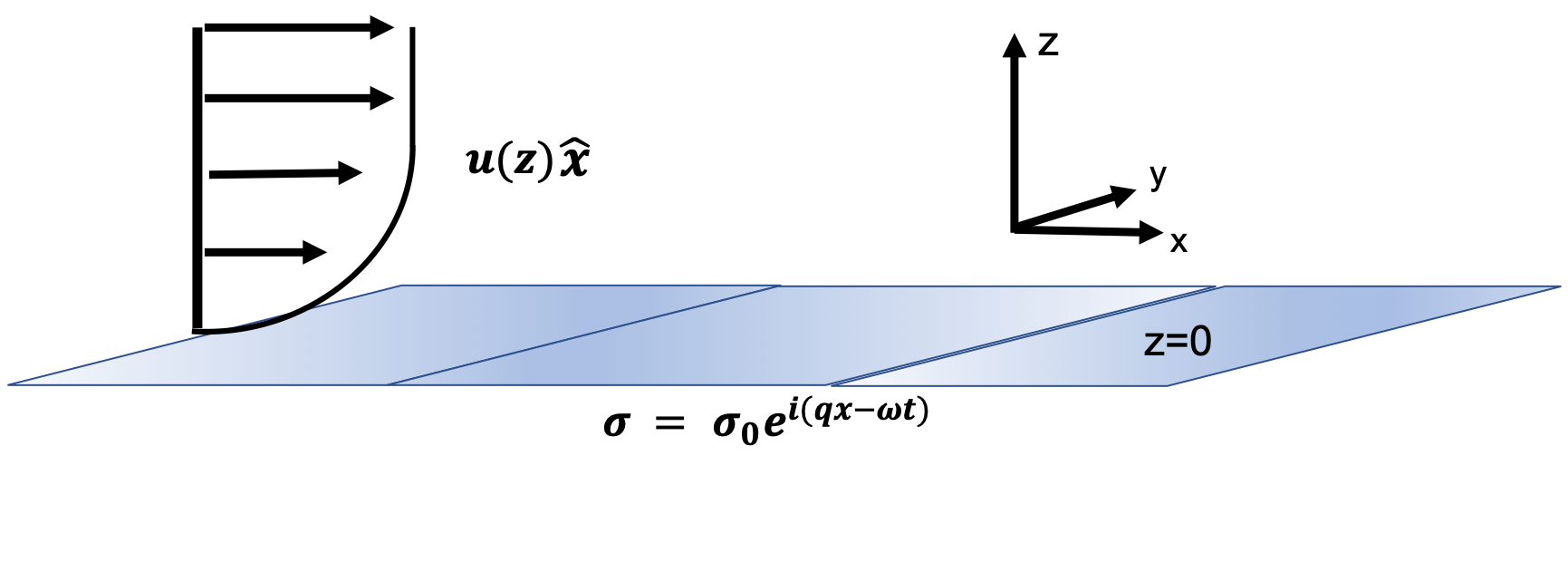
Figure 1: Nonlinear electroosmosis: Wall traveling wave charges give rise to a nonlinear body force and torque (see (9)) in a $1:1$ electrolyte lying in the semi-infinite space $z>0$, breaking the continuous $SO(2)$ symmetry of the system and leading to the appearance of a zero mode and a commensurate unidirectional fluid velocity in the $\hat{\mathbf{x}}$ direction, parallel to the channel walls, that is quadratic with respect to the associated electric field and that does not vanish after averaging over the charge period of oscillation.

4 Traveling wave nonlinear electroosmosis in a semi-infinite space

We consider the configuration displayed in Fig. 1. Traveling wave surface charges are applied on the wall $z=0$ bounding an $1:1$ electrolyte lying in the semi-infinite space $z>0$. The boundary conditions satisfied by the charge $\rho$ and potential $\phi$ at a solid surface simplify significantly. Since $\partial_{z}\phi(x,z=0)=-\frac{\sigma(x)}{\epsilon}$ (assuming the charged channel wall lies at $z=0$ and the vector normal to the wall ($\hat{\mathbf{z}}$) points in the $+z$ direction, into the electrolyte), the zero current condition $\mathbf{j}\cdot\hat{\mathbf{z}}=D\left[\nabla\rho+\frac{e}{k_{B}T}s\nabla\phi\right]\cdot\hat{\mathbf{z}}=0$ at the same wall leads to the requirement that $\partial_{z}\rho=\kappa^{2}\sigma(x)$. Thus, in summary, the boundary conditions satisfied by the potential and by the bulk charge are

$$\partial_{z}\phi(x,z=0,t)=-\frac{\sigma(x,t)}{\epsilon},\quad\partial_{z}\rho(x,z=0,t)=\kappa^{2}\sigma(x,t).$$ (10)

Assuming $\rho=\rho(z)e^{i(qx-\omega t)}$, Eq. (6) reduces to $\rho_{zz}+\left[i\omega/D-\kappa^{2}-q^{2}\right]\rho=0$ (in the low Péclet number limit) subject to $\rho_{z}=\kappa^{2}\sigma_{0}$ at $z=0$ and $\rho=0$ at infinity. To avoid clutter, we have introduced the notation $\rho_{z}\equiv\partial_{z}\rho$ etc.

The charge distribution reads

$$\rho(x,z,t)=-\frac{i\sigma_{0}\kappa^{2}}{P}e^{i(Pz+qx-\omega t)},$$ (11)

where

$$P\equiv P_{1}+iP_{2}=\sqrt{p^{2}-q^{2}-\kappa^{2}},\quad i\omega=Dp^{2},\quad p=\frac{1+i}{\Delta},\quad\Delta=\sqrt{\frac{2D}{\omega}}.$$ (12)

Quantity	Value	Definition
$\omega\;(\textrm{rad}\cdot\textrm{sec}^{-1})$	$10^{2}-10^{5}$	wall traveling wave charge frequency
$\Delta=\sqrt{\frac{2D}{\omega}}\;(\textrm{cm})$		charge penetration depth (cf. (12))
$q\;(\textrm{cm}^{-1})$	$0-10^{5}$	wall charge variation wavenumber
$\kappa\;(\textrm{cm}^{-1})$	$10^{2}-10^{5}$	inverse Debye length
$Q=\sqrt{q^{2}+\kappa^{2}}\;(\textrm{cm}^{-1})$
$p=\frac{1+i}{\Delta}\;(\textrm{cm}^{-1})$		charge oscillating complex wave number (cf. (12))
$P=\sqrt{p^{2}-q^{2}-\kappa^{2}}\;(\textrm{cm}^{-1})$		charge complex wave number (cf. (12))
$\eta$ ($\textrm{g}\>\textrm{cm}^{-1}\textrm{sec}^{-1}$)	$10^{-2}$	electrolyte dynamic viscosity
$\nu$ ($\textrm{cm}^{2}\textrm{sec}^{-1}$)	$10^{-2}$	electrolyte kinematic viscosity
$2h$ (cm)	$1-10^{-3}$	channel width
$a$ (cm)	$1-10^{-3}$	capillary radius
$u$ (cm/sec)	$0.1$	horizontal (zero mode) velocity component
$D\;(\textrm{cm}^{2}\textrm{sec}^{-1})$	$10^{-5}$	Diffusion coefficient for electrolyte charges
$\sigma,\sigma_{0}\;(\textrm{C/m}^{2})$		wall charge distribution
$E$ (V/m)	$10^{5}$	Electric field
$\epsilon$ (F/m)	$7\times 10^{-10}$	Dielectric constant
$\phi$		electric potential: $\mathbf{E}=-\nabla\phi$
$\psi$		streamfunction, cf. (7)
$\rho,s$		bulk charge and salt distribution
$\mathcal{P}$		hydrodynamic pressure

Table 1: Definitions of wavenumbers and parameter values. $\rho,q,Q,\sigma$ and $\kappa$ as in (Ajdari, 1995). $p$ and $\Delta$ correspond to the $k$ and $\delta$ of (Landau & Lifshitz, 1987, §24).

The notation employed in Eq. (12) for penetration depth $\Delta$ and complex wavenumber $p$ is analogous to (Landau & Lifshitz, 1987, p.84). These quantities here however refer to the wavelike form of the charge distribution away from a charged boundary, rather than the wavelike form of the velocity field away from a no-slip wall. Thus, in the absence of charge modulation ($q=0$) and double layer ($\kappa=0$) the charge diffuses away from the wall with penetration depth $\Delta$ (the inverse of the imaginary part of $p$) and oscillates with period $2\pi/\Delta$ away from the wall (the real part of $p$). This picture is also present when $\kappa$ and $q$ are non-zero. The penetration depth is now determined by the inverse of the imaginary part of $P$ (taken here to be positive) and there is an oscillation whose wavevector is the real part of $P$. In other words, if $P_{1}$ and $P_{2}$ denote the real and imaginary parts of $P$ in (12) ($P=P_{1}+iP_{2}$), where $P_{i}$ are real and $P_{2}>0$ then

$$P_{1,2}=\frac{1}{\sqrt{2}}\sqrt{\sqrt{\left(\kappa^{2}+q^{2}\right)^{2}+\frac{\omega^{2}}{\mathit{D}^{2}}}\mp(\kappa^{2}+q^{2})},$$ (13)

where the minus/plus sign corresponds to the real/imaginary part of $P$. Thus, the penetration depth is not determined by $2\pi/\kappa$ but by the length scale $2\pi/P_{2}>0$. With this notation, the charge distribution has the form

$$\rho(x,z,t)=-\frac{i\sigma_{0}\kappa^{2}}{P}e^{-P_{2}z}e^{i(P_{1}z+qx-\omega t)}.$$ (14)

Thus, in addition to the exponential decay away from the wall, the charge is modulated by a plane wave whose wavevector is not parallel to the surface charge distribution wave-vector (it is not parallel to the $x$-axis) in Eq. (3) but lies in the direction $q\hat{\mathbf{x}}+P_{1}\hat{\mathbf{z}}$.

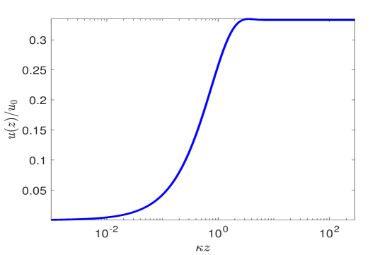
Figure 2: Depiction of the boundary layer of thickness (= penetration depth, see Eq. (12)) of $O(P_{2}^{-1})\sim\kappa^{-1}$ for large $\kappa$ employing (18). Beyond the boundary layer the liquid velocity rapidly acquires a constant value Following (Ehrlich & Melcher, 1982), the velocity has been scaled by $u_{0}=\frac{1}{2}\frac{\epsilon E^{2}}{\eta\kappa}$, and frequency by $D\kappa^{2}$, where $E=\frac{\sigma_{0}}{\epsilon}$ is the amplitude of the induced electric field due to the interfacial charge distribution $\sigma_{0}$, $\kappa^{-1},D,\eta$ are the Debye length, charge diffusion coefficient and liquid viscosity, respectively. Here we have taken $q=10^{3}\textrm{ cm}^{-1}$, $\kappa=10^{5}\textrm{ cm}^{-1}$ $D=10^{-5}\textrm{ cm}^{2}/$sec and $\omega=D\kappa^{2}$.

Similarly, assuming $\phi=\phi(z)e^{i(qx-\omega t)}$, Eq. (4) reduces to $\phi_{zz}-q^{2}\phi=\frac{i\sigma_{0}\kappa^{2}}{\epsilon P}e^{iPz},$ subject to the boundary condition (10) with surface charge (3) and $\phi=0$ at infinity (the alternative boundary condition of zero electric field at infinity leads to an identical result). Thus, the potential distribution reads

$$\phi(x,z,t)=\frac{\sigma_{0}}{\epsilon}\left(1+\frac{\kappa^{2}}{P^{2}+q^{2}}\right)\frac{e^{-qz}}{q}e^{i(qx-\omega t)}+\frac{1}{\epsilon(P^{2}+q^{2})}\rho,$$ (15)

with $\rho$ given by (14) and we assumed that $q>0$.

Note that with the Debye-Hückel approximation ($\rho=-\epsilon\kappa^{2}\phi$, everywhere), the first term on the right hand side (the term myltiplying $e^{-qz}$) vanishes, $P$ is real and the electric body force arising in the Navier-Stokes equations (2) vanishes identically, see Appendix A for a discussion of this point.

It is now clear that the nonlinear torque (last two terms in (9)) involves the harmonics $e^{\pm i\theta}$ and $e^{\pm 2i\theta}$ where $\theta=qx-\omega t$ and the commensurate streamfunction $\psi$ satisfying (9) will also be composed of the same harmonics. Thus, the velocity vanishes when averaged over the period $2\pi/\omega$ of oscillations.

There is however a part of the nonlinear torque in (9) that is time-independent and does not vanish when averaged over the period of oscillations. This is caused by constructive interference of the various harmonics expressing the charge and potential distribution in (14) and (15), respectively and gives rise to unidirectional pumping of liquid, its direction determined by the propagation direction of the charge distribution lying on the walls. We now investigate this zero mode.

Let $\psi=\psi(z)$, and thus the velocity $\mathbf{v}=u(z)\hat{\mathbf{x}}$ (where both $\psi$ and $u$ are real fields), cf. Fig. 1. In Appendix B we show that after averaging over the period of oscillation, the vorticity equation (9) reduces to

$$\partial_{z}u(z)=\frac{i\epsilon q}{4\eta}\left(\phi^{*}\phi_{z}-\phi\phi_{z}^{*}\right),$$ (16)

where a star denotes the complex conjugate of (15). It is clear that the complex exponentials $e^{i(qx-\omega t)}$ have canceled-out. This is the central formula of this paper. (We also verify the validity of this expression by starting directly from the Navier-Stokes equations which after averaging over the period of oscillation reduce to (2), see Appendix C).

It is thus easy to determine the horizontal velocity component $u(z)$. Employing the complex form of the field $\phi$ in (15) we solve (16) subject to the boundary conditions

$$u(z=0)=0,\quad u(z=\infty)=\textrm{finite}.$$ (17)

With these boundary conditions the zero mode velocity $u(z)$ from (16) with (15) becomes symbolically

$$u(z)=\frac{i\epsilon q}{4\eta}\int_{0}^{z}\left(\phi^{*}\phi_{z}-\phi\phi_{z}^{*}\right)dz.$$ (18)

The zero mode (18) inherits the boundary-layer structure of the field $\phi$ as displayed in Fig. 2. A boundary layer of thickness $O(P_{2}^{-1})\sim\kappa^{-1}$ for large $\kappa$ separates the no-slip region at the wall to the constant value acquired by the velocity away from the wall.

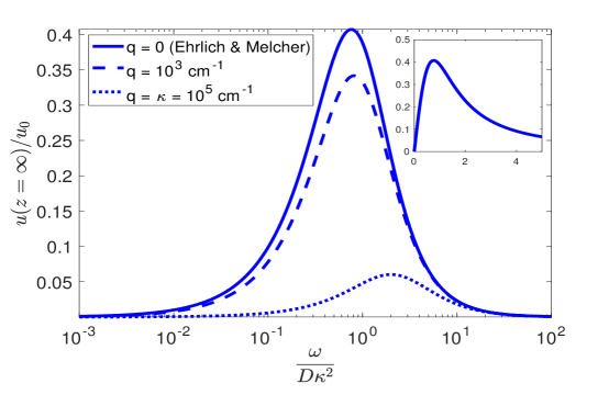
Figure 3: Horizontal zero-mode velocity $u(z)$ evaluated at $z=\infty$, from Eq. (18) as a function of the frequency of the traveling wave wall charge. The continuous curve depicts the zero mode with infinite wall charge wavelength modulation $q=0$, recovering the result of (Ehrlich & Melcher, 1982, Eq. (34)), which is reproduced in the inset in linear axes (Ehrlich & Melcher, 1982, Fig. 3). Following (Ehrlich & Melcher, 1982), the velocity has been scaled by $u_{0}=\frac{1}{2}\frac{\epsilon E^{2}}{\eta\kappa}$, and frequency by $D\kappa^{2}$, where $E=\frac{\sigma_{0}}{\epsilon}$ is the amplitude of the induced electric field due to the interfacial charge distribution $\sigma_{0}$, $\kappa^{-1},D,\eta$ are the Debye length, charge diffusion coefficient and liquid viscosity, respectively. Here we have taken $\kappa=10^{5}\textrm{ cm}^{-1}$ and $D=10^{-5}\textrm{ cm}^{2}/$sec.

In the present semi-infinite space formulation, the observable of interest is the value taken by the electrolyte velocity zero mode (18) at $z=\infty$. It reads

$$u(\infty)=\frac{\kappa^{3}\left(R^{3}\sin\!4\Theta-R\left(R^{2}-\kappa^{2}+q^{2}\right)\sin\!2\Theta-q\left(2R^{2}-\kappa^{2}\right)\cos\!\Theta+2R^{2}q\cos\!3\Theta\right)}{2R^{2}(R^{2}q^{2}\sin\!3\Theta-(R^{4}+5R^{2}q^{2}+q^{4})\sin\!\Theta-2Rq(R^{2}+q^{2})(1-\cos\!2\Theta))}$$ (19)

where, following (Ehrlich & Melcher, 1982), the horizontal velocity $u$ was scaled by $u_{0}=\frac{1}{2}\frac{\epsilon E^{2}}{\eta\kappa}$, where $E=\frac{\sigma_{0}}{\epsilon}$ is the electric field amplitude due to the interfacial charge distribution $\sigma_{0}$ (and for simplicity we chose the sign $q>0$). Here $R$ and $\Theta$ are the amplitude and phase of the complex wavenumber $P=Re^{i\Theta}$ defined in (12) and given explicitly by

$$R={\left(\left(\kappa^{2}+q^{2}\right)^{2}+\frac{\omega^{2}}{\mathit{D}^{2}}\right)}^{\frac{1}{4}},\quad\Theta=-\frac{1}{2}\arctan\!\left(\frac{\omega}{\mathit{D}\left(\kappa^{2}+q^{2}\right)}\right)+\frac{\pi}{2}.$$ (20)

To increase clarity, we will follow the notation of (Ehrlich & Melcher, 1982) by introducing the timescale (in their notation)

$$t_{e}\equiv\frac{\epsilon k_{B}T}{2c^{\infty}eD}=\frac{1}{D\kappa^{2}},$$ (21)

where $\kappa$ was defined in (8). With this notation, the amplitude and phase in (20) become

$$R=\sqrt{\kappa^{2}+q^{2}}\left[1+\left(\frac{\omega t_{e}}{1+\left(\frac{q}{\kappa}\right)^{2}}\right)^{2}\right]^{\frac{1}{4}},\quad\Theta=-\frac{1}{2}\arctan\left(\frac{\omega t_{e}}{1+\left(\frac{q}{\kappa}\right)^{2}}\right)+\frac{\pi}{2}.$$ (22)

A special case of the above formalism that has appeared before in the literature, can be recovered by substituting (22) into (19) and setting $q=0$. We thus arrive at

$$u(\infty)=\frac{\omega t_{e}}{\left(\omega^{2}t_{e}^{2}+1\right)^{\frac{5}{4}}}\cos\!\left(\frac{\arctan\left(\omega t_{e}\right)}{2}\right),$$ (23)

which is Eq. (34) of (Ehrlich & Melcher, 1982) and $t_{e}$ was defined in (21). In Fig. 3 we display the zero mode (19) with (22) for various values of the wall charge modulation wavevector $q$. The continuous curve denotes the $q=0$ mode which recovers Fig. 3 of (Ehrlich & Melcher, 1982) in logarithmic axes and in the inset in linear axes.

Although Eq. (23) has an appealing form, it is misleading, as it is unclear what the mechanism is that drives the flow in the electrolyte. The $q=0$ limit, upon which (23) depends, does not distinguish a vector quantity which, upon reversal, will drive the electrolyte in the opposite direction. We thus proceed to analyze this paradox.

When the sign of $q$ is unspecified the charge and potential expressions in (14) and (15), respectively, remain unchanged by effecting the replacement $q\rightarrow|q|$. Substituting these two relations into (16) and taking the limit of small $q$ leads to the conclusion that

$$u(z)\sim\frac{q}{|q|},\quad\textrm{as}\quad q\rightarrow 0.$$ (24)

To be more specific, the zero mode velocity (19) at $z=\infty$ is replaced by a very long expression, which, in the limit of small $q$ reduces to

$$u(\infty)\sim\frac{q}{|q|}\kappa^{3}\frac{R^{2}\sin 4\Theta-(R^{2}-\kappa^{2})\sin 2\Theta}{2R^{5}\sin\Theta},\quad\textrm{as}\quad q\rightarrow 0,$$ (25)

where $R$ and $\Theta$ are given by (20) by setting $q=0$. The meaning of the $q=0$ solution in (23) is now clear. It is a singular limit in that the solution $u$ is discontinuous at $q=0$, two solutions exist at $q=0$, and thus the solution is non-unique. (23) is one of the two solutions as $q=0$ is approached from positive $q$ values. This could have been anticipated from the form of the potential (15) which becomes infinite at $q=0$. Another way to see this is to start from first principles and pursue the solution of the boundary value problem for $q=0$. Then, the potential $\phi$ cannot satisfy both boundary conditions, while the absence of $x$-dependence in the electric body force or torque in (9) points to the absence of a driving mechanism. Note that the foregoing discussion implies that a uniform distribution of surface charges lying on the bounding wall does not give rise to a zero mode velocity and to a unidirectional liquid pumping.

In general, the flow velocity is proportional to $q$ whose sign reversal leads the electrolyte to move in the opposite direction as would be expected from symmetry arguments. Under spatial inversion $(x,z)\rightarrow(-x,-z)$, the electric field $(-\phi_{x},-\phi_{z})$ changes sign and the same is true for the velocity (as long as $q$ also changes sign). This can be seen directly from Eq. (16).

It is worthwhile to note that the wavenumber $P$ and charge and analogous expressions for the potential distributions (14) and (15) (satisfying fixed potential boundary conditions) have appeared before in (Mortensen et al., 2005) (their equations (18b) and (18a) and (20), respectively), where an insulator at $z\in(-d,0)$ separates an electrolyte (at $z>0$) and a conductor (at $z<-d$). Therein, it was shown that certain approximations leading to the “capacitor model” gave rise to a vanishing time-average electrolyte velocity, and this disagreed with the predictions obtained by solving the full system numerically showing the presence of a non-zero pumping velocity in the same reference. This discrepancy can be explained by substituting their equations (24) and (25) into our (16) and (18) (which are independent of charge and potential boundary conditions), leading the electrolyte velocity to vanish. The approximations employed in (Mortensen et al., 2005) have discarded the (corresponding) last term in the potential expression (15). Its presence would lead to constructive interference of the various harmonics and to the pressence of a zero velocity mode, thus agreeing with their full numerical simulations.

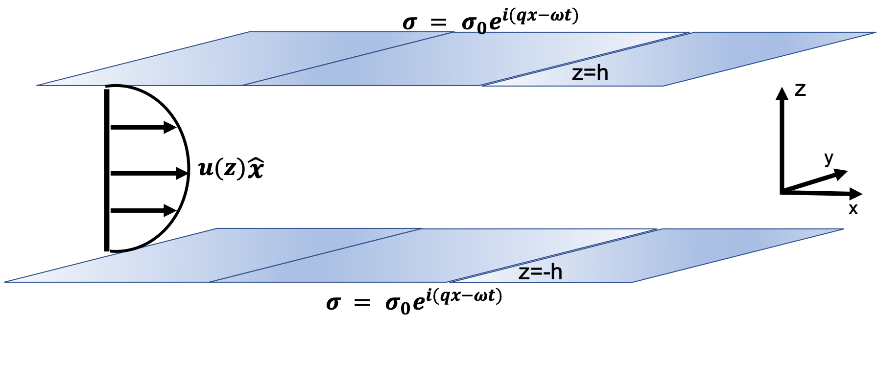
Figure 4: Nonlinear electroosmosis: Traveling wave surface charges give rise to a nonlinear body force and torque (see (9)) in a $1:1$ electrolyte in a rectangular channel of width $2h$ breaking the continuous $SO(2)$ symmetry of the system and leading to the appearance of a zero mode and a commensurate unidirectional fluid velocity in the $\hat{\mathbf{x}}$ direction, parallel to the channel walls that is quadratic with respect to the associated electric field and that does not vanish after averaging over the charge period of oscillation.

5 Traveling wave nonlinear electroosmosis in a channel of width $2h$

Instead of the nonlinear electroosmosis taking place in a semi-infinite space as developed in section 4, it is more physically realistic to consider the configuration displayed in Fig. 4. Traveling wave surface charges are applied on the channel walls at $z=\pm h$ enclosing an $1:1$ electrolyte. The boundary conditions satisfied by the potential $\phi$ and by the charge $\rho$ are

$$\partial_{z}\phi(x,z=\pm h,t)=\pm\frac{\sigma^{\pm}(x,t)}{\epsilon},\quad\partial_{z}\rho(x,z=\pm h,t)=\mp\kappa^{2}\sigma^{\pm}(x,t),$$ (26)

with $\sigma^{\pm}=\sigma_{0}e^{i(qx-\omega t)}$. Assuming $\rho=\rho(z)e^{i(qx-\omega t)}$ and subject to the boundary condition (26) with surface charge (3) the equations to solve are identical to those of the semi-infinite space. Thus, the charge distribution reads

$$\rho(x,z,t)=-\frac{\sigma_{0}\kappa^{2}\cos Pz}{P\sin Ph}e^{i(qx-\omega t)},$$ (27)

where $P$ is the complex wavenumber displayed in (12). Note that this form of bulk charge distribution does not violate electroneutrality. The denominator of expression (27) is composed of hyperbolic functions of large argument (since $P$ is complex) so, close to the center of the channel ($z=0$) the charge is effectively zero, cf. (Ajdari, 1995, Eq. (4)) for the corresponding case of a steady periodic wall charge distribution.

Similarly, assuming $\phi=\phi(z)e^{i(qx-\omega t)}$ and subject to the boundary condition (26) with surface charge (3), the potential distribution reads

$$\phi(x,z,t)=\frac{\sigma_{0}}{\epsilon}\left(1+\frac{\kappa^{2}}{P^{2}+q^{2}}\right)\frac{\cosh qz}{q\sinh qh}e^{i(qx-\omega t)}+\frac{1}{\epsilon(P^{2}+q^{2})}\rho,$$ (28)

with $\rho$ given by (27).

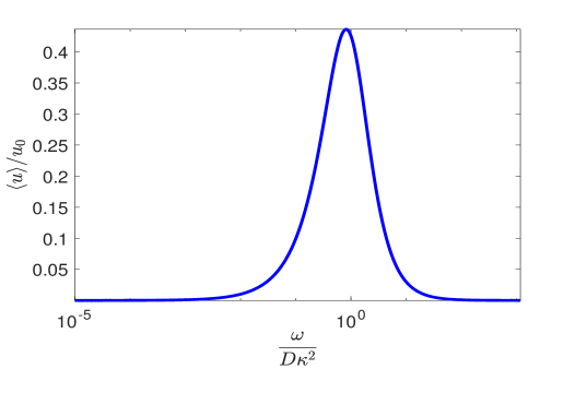
Figure 5: Zero mode velocity (31), averaged over the channel width $2h$. Following (Ehrlich & Melcher, 1982), the velocity has been scaled by $u_{0}=\frac{1}{2}\frac{\epsilon E^{2}}{\eta\kappa}$, and frequency by $D\kappa^{2}$, where $E=\frac{\sigma_{0}}{\epsilon}$ is the amplitude of the induced electric field due to the interfacial charge distribution $\sigma_{0}$, $\kappa^{-1},D,\eta$ are the Debye length, charge diffusion coefficient and liquid viscosity, respectively. Here we have taken $q=10^{3}\textrm{ cm}^{-1}$, $\kappa=10^{4}\textrm{ cm}^{-1}$ $D=10^{-5}\textrm{ cm}^{2}/$sec, $h=10^{-3}$ cm and $\omega=D\kappa^{2}$.

The zero mode velocity in the channel again satisfies the integrated momentum Eq. (16). Employing the complex form of the field $\phi$ in (28) we thus solve (16) subject to the no-slip boundary conditions

$$u(z=\pm h)=0.$$ (29)

The zero mode velocity $u(z)$ from (16) with (28) becomes symbolically

$$u(z)=\frac{i\epsilon q}{4\eta}\int_{h}^{z}\left(\phi^{*}\phi_{z}-\phi\phi_{z}^{*}\right)dz$$ (30)

(the constant of integration vanishes since $\phi$ is an even function of $z$ with respect to the origin $z=0$). Following the same steps as in the semiinfinite space of section 4, leads to a long and uninformative expression for $u(z)$. This is essentially a plug-like flow with very thin boundary layers of thickness $\sim\kappa^{-1}$ located at $z=\pm h$. The meaningful observable here is the average value of the zero mode over the width of the channel

$$\langle u\rangle=\frac{1}{2h}\int_{-h}^{h}{u(z)}dz.$$ (31)

Following (Ehrlich & Melcher, 1982), we will scale the velocity by $u_{0}=\frac{1}{2}\frac{\epsilon E^{2}}{\eta\kappa}$, where $E=\frac{\sigma_{0}}{\epsilon}$ is the amplitude of the electric field due to the interfacial charge distribution $\sigma_{0}$. In figure 5 we display the zero mode velocity averaged over the channel width (31) versus the frequency of charge oscillation $\omega$ scaled by the frequency $D\kappa^{2}$, where $D$ is the diffusion coefficient of the charge distribution. As it stands, (31) is a double integral and could be awkward to evaluate, especially in cylindrical polars (see section 6). It can be significantly simplified by changing the order of integration and carrying-out one of the integrations. It can thus be written as a single integral in the form

$$\langle u\rangle=-\frac{1}{2h}\frac{i\epsilon q}{4\eta}\int_{-h}^{h}\left(\phi^{*}\phi_{z}-\phi\phi_{z}^{*}\right)zdz,$$ (32)

where the parity of $\phi$ with respect to the origin $z=0$ was taken into account.

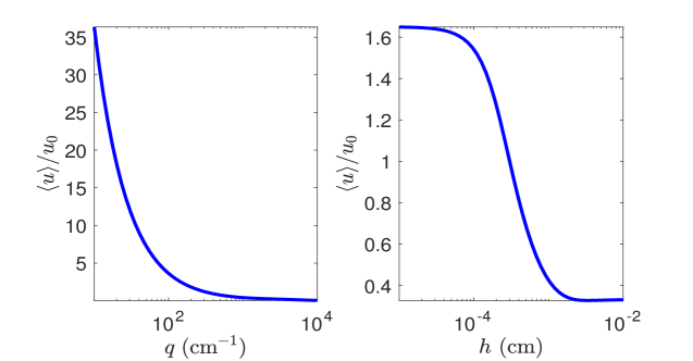
Figure 6: Left panel: Variation of the zero mode (31), averaged over the channel width, with wavevector $q$ of the wall charge modulation ($h=10^{-3}\textrm{ cm}$), which displays the diverging character of the velocity as $q\rightarrow 0$, discussed in Eq. (33). Right panel: Variation of the zero mode velocity (31), (averaged over the channel width), with the half-width of the channel $h$, ($q=10^{3}\textrm{ cm}^{-1}$), displaying the constant character of the velocity as $h\rightarrow 0$, discussed in Eq. (34). Following (Ehrlich & Melcher, 1982), the velocity has been scaled by $u_{0}=\frac{1}{2}\frac{\epsilon E^{2}}{\eta\kappa}$, and frequency by $D\kappa^{2}$, where $E=\frac{\sigma_{0}}{\epsilon}$ is the amplitude of the induced electric field due to the interfacial charge distribution $\sigma_{0}$, $\kappa^{-1},D,\eta$ are the Debye length, charge diffusion coefficient and liquid viscosity, respectively. Here we have taken, $\kappa=10^{4}\textrm{ cm}^{-1}$ $D=10^{-5}\textrm{ cm}^{2}/$sec, $h=10^{-3}$ cm and $\omega=D\kappa^{2}$.

Two limits are of interest. First taking the limit of small $q$ we obtain from (31)

$$\langle u\rangle\sim\frac{1}{q},\quad\textrm{as}\quad q\rightarrow 0.$$ (33)

This is a singular limit and in fact, the boundary value problem has no solution when $q=0$ since the electric potential cannot satisfy both boundary conditions (and in addition, since the fields become independent of $x$ in this limit, leads the torque in (9) or the electric body force in the Navier-Stokes equations to vanish). Left panel of figure 6 displays the variation of the channel width-averaged zero mode (31) with the charge variation wavevector $q$. It is evident that the divergence (33) is present. This conclusion is reminiscent of (Cahill et al., 2004, Fig. 6(a)), although their boundary conditions are different to ours and their theoretical formulation is based on a semi-infinite space.

Second, the question arises, how the averaged (zero mode) velocity (31) depends on the width of the channel. In this case asymptotic expansions show that

$$\langle u\rangle\sim\textrm{constant}\quad\textrm{as}\quad h\rightarrow 0.$$ (34)

The right panel of figure 6 displayes this asymptotic behavior of the average velocity as $h\rightarrow 0$.

6 Traveling wave nonlinear electroosmosis in a cylindrical capillary

A still more physically realistic configuration is displayed in Fig. 4. Traveling wave surface charges $\sigma=\sigma_{0}e^{i(qx-\omega t)}$ are applied to the wall of a capillary with circular cross-section of radius $a$, enclosing an $1:1$ electrolyte. The boundary conditions satisfied by the potential $\phi$ and by the charge $\rho$ are

$$\partial_{r}\phi(x,r=a,t)=\frac{\sigma(x,t)}{\epsilon},\quad\partial_{r}\rho(x,r=a,t)=-\kappa^{2}\sigma(x,t),$$ (35)

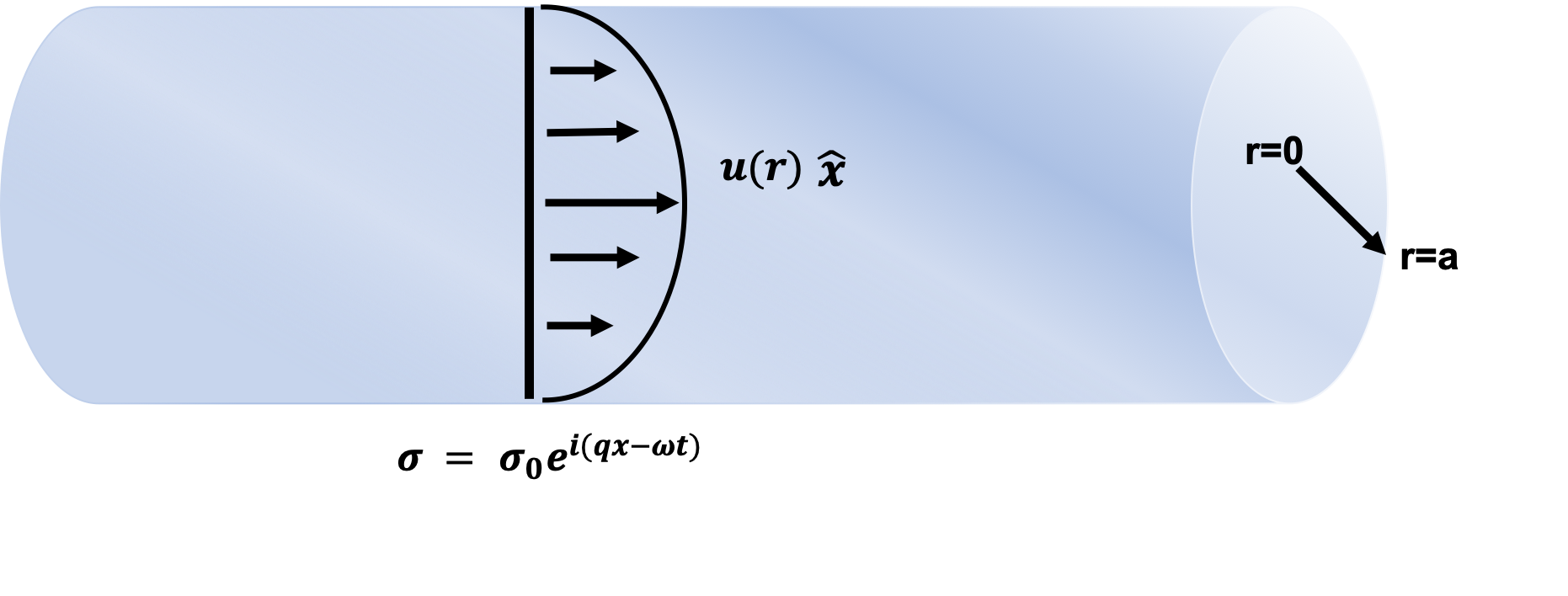
Figure 7: Nonlinear electroosmosis: Traveling wave surface charges give rise to a nonlinear body force and torque (see (9)) in a $1:1$ electrolyte in a cylindrical capillary of radius $a$ breaking the continuous $SO(2)$ symmetry of the system and leading to the appearance of a zero mode and a commensurate unidirectional fluid velocity in the $\hat{\mathbf{x}}$ direction, along the capillary center axis, that is quadratic with respect to the associated electric field and that does not vanish after averaging over the charge period of oscillation.

and we take the axis of the cylinder to lie in the $x$- direction as displayed in Fig. 7. Assuming $\rho=\rho(r)e^{i(qx-\omega t)}$ and $\phi=\phi(r)e^{i(qx-\omega t)}$, the evolution equation for the charge and Gauss law reduce to

$$\rho_{rr}+\frac{1}{r}\rho_{r}+\left[\frac{i\omega}{D}-q^{2}-\kappa^{2}\right]\rho=0,\quad\textrm{and}\quad\phi_{rr}+\frac{1}{r}\phi_{r}-q^{2}\phi=-\frac{\rho}{\epsilon},$$ (36)

respectively. With boundary conditions (35), we obtain

$$\rho(x,r,t)=-\frac{\sigma_{0}\kappa^{2}J_{0}(Pr)}{PJ_{1}(Pa)}e^{i(qx-\omega t)},$$ (37)

where $P$ is (again) the complex wavenumber displayed in (12) and $J_{0}$ and $J_{1}$ are Bessel functions of the first kind. As in the case of the channel, Eq. (37) does not violate electroneutrality, see the discussion below (27). Likewise, subject to the boundary condition (35), the potential distribution reads

$$\phi(x,r,t)=\frac{\sigma_{0}}{\epsilon}\left(1+\frac{\kappa^{2}}{P^{2}+q^{2}}\right)\frac{I_{0}(qr)}{qI_{1}(qa)}e^{i(qx-\omega t)}+\frac{1}{\epsilon(P^{2}+q^{2})}\rho,$$ (38)

with $\rho$ given by (37) and $I_{0}$ and $I_{1}$ are modified Bessel functions of the first kind (Bessel functions of imaginary argument).

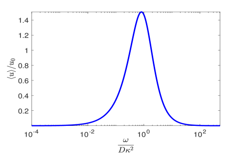
Figure 8: Nonlinear electroosmosis in a cylinder, cf. Fig. 7, with traveling wave charge distribution. Zero mode (43), averaged over the cross-sectional area of the cylinder of radius $a$. Following (Ehrlich & Melcher, 1982), the velocity has been scaled by $u_{0}=\frac{1}{2}\frac{\epsilon E^{2}}{\eta\kappa}$, and frequency by $D\kappa^{2}$, where $E=\frac{\sigma_{0}}{\epsilon}$ is the amplitude of the induced electric field due to the interfacial charge distribution $\sigma_{0}$ and $\kappa^{-1},D,\eta$ are the Debye length, charge diffusion coefficient and liquid viscosity, respectively. Same parameter values as the left panel of Fig. 5 and cylinder radius $a=10^{-3}$ cm.

As before, the velocity field consists of terms that vanish after averaging over the period of oscillation of the fields. The exception is the zero-mode velocity, satisfying an equation analogous to (16). Starting from the Navier-Stokes equations (where only the time-independent terms are retained) and considering the velocity field to have the form $\mathbf{v}=u(r)\hat{\mathbf{x}}$ (as displayed in Fig. 7), we obtain

$$u_{rr}+\frac{1}{r}u_{r}+\frac{iq}{4\eta}(\rho\phi^{*}-\rho^{*}\phi)=0.$$ (39)

Using the second of (36) and performing one integration we arrive at

$$\partial_{r}u(r)=\frac{i\epsilon q}{4\eta}\left(\phi^{*}\phi_{r}-\phi\phi_{r}^{*}\right)$$ (40)

which is the cylindrical counterpart of (16). Employing the complex form of the field $\phi$ in (38) we thus solve (40) subject to the no-slip boundary condition

$$u(r=a)=0.$$ (41)

The zero mode velocity $u(r)$ from (40) with (38) becomes symbolically

$$u(r)=\frac{i\epsilon q}{4\eta}\int_{a}^{r}\left(\phi^{*}\phi_{r}-\phi\phi_{r}^{*}\right)dr,$$ (42)

which is the cylindrical counterpart of (18) and (30) (the constant of integration is zero to maintain $\partial_{r}u|_{r=0}=0$. Otherwise the flow would have a cusp (discontinuous derivative of $u$) at $r=0$). The same steps followed in the semi-infinite space problem of section 4, lead to a long expression for $u(r)$ which is a plug-like flow with very thin boundary layers of thickness $\sim\kappa^{-1}$ located at the cylinder wall $r=a$. The meaningful observable here is the average value of the zero mode over the capillary cross-sectional area, leading to the definition

$$\langle u\rangle=\frac{1}{\pi a^{2}}\int_{0}^{a}{u(r)}2\pi rdr,$$ (43)

where $u(r)$ is given by (42). This latter expression involves indefinite integrals of Bessel function pairs which, in general, cannot be calculated in closed form (for exceptions, see for instance (Erdélyi et al., 1953, 1955; Luke, 1962)). We circumvent this complication by exchanging the order of integration in the double integral appearing in Eq. (43). Thus, (43) can be written as a single integral

$$\langle u\rangle=\frac{-2}{a^{2}}\int_{0}^{a}\left(\phi^{*}\phi_{r}-\phi\phi_{r}^{*}\right)r^{2}dr,$$ (44)

and is calculated numerically by simple quadrature. As we have done earlier, following (Ehrlich & Melcher, 1982), we scale the velocity by $u_{0}=\frac{1}{2}\frac{\epsilon E^{2}}{\eta\kappa}$, where $E=\frac{\sigma_{0}}{\epsilon}$ is the amplitude of the electric field due to the interfacial charge distribution $\sigma_{0}$. In figure 8 we display the zero mode velocity averaged over the channel width (44) versus the frequency of charge oscillation $\omega$ scaled by the frequency $D\kappa^{2}$, where $D$ is the diffusion coefficient of the charge distribution.

7 Validity of the charge perturbation approximation

It is instructive to examine the conditions under which the reduction of the charge evolution equation (6) and associated boundary condition was possible. The requirement is that $\rho\ll 2c^{\infty}$.

For the semi-infinite space, Eq. (14) and (20) lead to the requirement

$$Re\left\{\frac{\sigma_{0}\kappa^{2}}{P}\right\}<\frac{\sigma_{0}\kappa^{2}}{R}\equiv\frac{\epsilon E\kappa^{2}}{\left[(\kappa^{2}+q^{2})^{2}+\left(\frac{\omega}{D}\right)^{2}\right]^{\frac{1}{4}}}\ll 2c^{\infty},$$ (45)

and this is analogous (but not identical) to the criterion reported by (Ehrlich & Melcher, 1982, below their Fig. 5) for the $q=0$ case. This condition then poses an upper bound on the electric field amplitude in such a semi-infinite space.

Eq. (45) can be reexpressed more clearly by eliminating $c^{\infty}$ in favor of $\kappa$ through (8)

$$f(\kappa,E)\equiv\frac{eE}{k_{B}T\left[(\kappa^{2}+q^{2})^{2}+\left(\frac{\omega}{D}\right)^{2}\right]^{1/4}}\ll 1.$$ (46)

In the left two panels of figure 9 we plot contours of the function $f(\kappa,E)$ in (46) for the constant values $f=1,0.1,0.01$ and $0.001$ for $q=10^{3}\;\textrm{cm}^{-1}$, and $D=10^{-9}\;\textrm{m}^{2}/\textrm{sec}$ at room temperature. It is thus seen that the range of validity of the approximation increases as the frequency $\omega$ (or the ratio $\omega/D$) increases: Left-most panel: $\omega=10^{2}$ rad/sec. Middle panel: $\omega=10^{5}$ rad/sec.

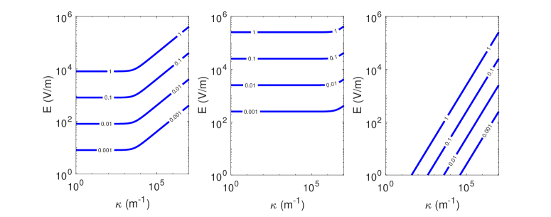
Figure 9: Validity of the charge perturbation approximation is established when $f(\kappa,E)\ll 1$ (cf. Eq. (46)). Leftmost panels: contour plot of the function $f(\kappa,E)$ in (46) for the constant values $f=1,0.1,0.01$ and $0.001$ for $q=10^{3}\;\textrm{cm}^{-1}$, and $D=10^{-9}\;\textrm{m}^{2}/\textrm{sec}$ at room temperature. It is thus seen that the range of validity of the approximation increases as the frequency $\omega$ (or the ratio $\omega/D$) increases: Left-most panel: $\omega=10^{2}$ rad/sec. Middle panel: $\omega=10^{5}$ rad/sec. Rightmost panel: contour plot of the function $\frac{eE}{\kappa k_{B}T}$ in (47) (the large $\kappa$ limit of $f(\kappa,E)$) at room temperature. The condition (47) resembles the corresponding requirement for the validity of the Debye-Hückel approximation (see discussion in the text).

In the small Debye length limit Eq. (45) becomes $\sigma_{0}\kappa\ll 2c^{\infty}$. Eliminating $c^{\infty}$ (or taking the large $\kappa$ limit in (46)) we obtain the following bound

$$\frac{eE}{\kappa k_{B}T}\ll 1.$$ (47)

This is analogous to the Debye-Hückel approximation where $e\phi\ll k_{B}T$ (Melcher, 1981, p. 10.22), if the characteristic length-scale of the system is the Debye length. In the right-most panel of figure 9 we plot contours of the function $\frac{eE}{\kappa k_{B}T}$ at room temperature. Clearly the range of validity of the approximation leading to the bound (46) and displayed in the two leftmost panels of figure 9, is superior.

7.1 Estimates

The foregoing discussion demonstrates that the zero mode velocity is much larger in channels and capillaries in comparison to its semi-infinite space counterpart. For instance, figures 5 and 8 show that there are frequency intervals where the scaled velocity is of order one. Of course, when the remaining parameters are also varied, can lead to even higher scaled velocities. For the sake of simplicity we will assume that the parameters are so chosen as to make the scaled velocity of $O(1)$. Thus, an estimate of the dimensional zero-mode velocity in a channel or cylindrical capillary is

$$u\sim u_{0}=\frac{1}{2}\frac{\epsilon E^{2}}{\eta\kappa}.$$ (48)

Employing standard parameter values for water $\epsilon=7\times 10^{-10}$ F/m, $\eta=0.001$ kg/m sec, $\kappa=10^{6}\textrm{ m}^{-1}$ and $E=10^{5}$ V/m we obtain the estimate

$$u\sim 3.5\textrm{ mm/sec}.$$ (49)

This estimate is of the same order of magnitude as the numerical results of (Ehrlich & Melcher, 1982) and can be considered as an upper bound of recent experimental measurements (Yen et al., 2019).

8 Discussion

In this paper we considered the effect of the nonlinear electric body force induced by wall traveling wave charges and exerted on an electrolyte. Although, in general, the flow patterns vanish after averaging over the period of oscillation, constructive interference leads to the appearance of a zero mode velocity, that is, a flow velocity field that is time-independent and whose direction depends on the wall charge modulation wavevector $\mathbf{q}$. In this sense, this nonlinear effect can drive an electrolyte in a semiinfinite space or in a channel with parallel walls, without invoking an asymmetric geometrical configuration, eg. a conically shaped capillary cf. (Kamsma et al., 2023). We showed that the $q\rightarrow 0$ limit is singular as it is not associated with a specific direction of a driving mechanism.

There is great efficiency present in the zero mode nonlinear electroosmosis mechanism in comparison to pumping through pressure gradients. In the latter, the velocity decreases as the size of the channel decreases. Here, the velocity increases until it reaches a steady limit (cf. Fig. 6 and Eq. (34)). In addition there is great flexibility as the conditions set by our approximation on the electric field amplitude can be very modest as the discussion in section 7 demonstrates.

In the work of Ehrlich & Melcher (1982) it was shown that the “small field” theory overestimates the velocity obtained by full numerical simulations (see Fig. 8 in Ehrlich & Melcher (1982)). We’ve seen here that a judicious choice of the wall charge wavenumber $q$ can give rise to a decrease in the zero-mode velocity magnitude. In addition the theoretical results of Ehrlich & Melcher (1982) are based on the semi-infinite space theory. We have shown here that results of such a semi-infinite space analysis may differ in character and magnitude from the channel and cylindrical capillary theory and in particular, they are very much pronounced in the two latter cases compared to the semi-infinite space results.

What we have not addressed is the effect of the flow on the charge distribution, that is the role played by the (nonlinear) advection terms that appear in the charge distribution evolution equation (6). We anticipate that inclusion of these nonlinear terms into our formalism, will give rise to a number of additional effects such as a back flow or velocity reversal in certain spatial domains. A corresponding numerical investigation of some of these effects can be traced back to the work of Ehrlich & Melcher (1982).

In this paper we employed boundary conditions the electric potential has to satisfy that are of von Neumann-type (it is the surface charge specified on the walls and this fixes the normal derivative of the potential on the boundary). The same analysis can easily be duplicated with Dirichlet boundary conditions where it is the electric potential that is fixed on the bounding walls. The two results are qualitatively different with respect to variations of the wavenumber $q$, but both give rise to a zero velocity mode.

Setting $\omega=0$ and repeating gives $\rho=-\epsilon\kappa^{2}\phi$ and the nonlinear torque vanishes identically. Then, with $\cos qx$ wall charge, electroosmosis exists only by applying an external field, thus recovering the results of (Ajdari, 1995).

Some comments regarding the status of this paper, within a literature as vast as the one of electroosmosis, are at place here. Most works of electroosmosis consider the semi-infinite space formulation, which, although useful, is not sometimes representative of a real physical situation. Here we consider this semi-infinite space case and how it contrasts to the nonlinear electroosmosis problem in a channel and in a cylindrical capillary. The zero mode velocity obtained in the two latter cases is more pronounced compared to their semi-infinite domain counterpart. Further, we have considered a minimal but clear presentation that makes connections with the oscillating viscous liquids literature as this is described in a standard reference of fluid mechanics (Landau & Lifshitz, 1987, p.89), and we follow its notation and its philosophy as far as this is possible, in order to assist the reader. As commented by Levich (1962), there is a need to describe effects in physicochemical hydrodynamics in a manner approachable by physicists and neglect, at least at first reading, the vast and diverse circumstances that “tend to burden it (the subject) with details that have no direct bearing on the essentials of the situation” (Levich, 1962, p. 231). We thus follow this philosophy in this paper. It should be easy to adopt this formulation to problems that would employ alternative boundary conditions such as fixed potentials on the capillary wall. The main formulas describing the zero mode in the symbolic form (30) and (42) and the reduced integrated form of the Navier-Stokes equations in (16) and (40) will remain unchanged.

Appendix A Approximation leading to Eq. (6)

We briefly interject here to discuss the effect of the approximation that leads to the form (6) for the evolution of the charge distribution. Dropping the time-dependence and nonlinear terms, shows that the relation between charge and potential in the bulk of the liquid is

$$\nabla^{2}(\rho+\epsilon\kappa^{2}\phi)=0.$$ (50)

On the other hand, the small potential (Debye-Hückel) approximation employed in the vast majority of the literature leads to the following potential-charge relation in the bulk of the liquid

$$\rho+\epsilon\kappa^{2}\phi=0,$$ (51)

where both (50) and (51) satisfy the boundary condition $\rho+\epsilon\kappa^{2}\phi=0$. (51) can be considered as a special case of (50). The two cases differ by a harmonic function which can have significant effects on whether the field can satisfy certain boundary conditions.

Appendix B Simplification of the nonlinear torque in (9)

In this Appendix we reduce the fourth order vorticity equation (9) to the first order (16).

Let

$$2\rho=\rho(z)e^{i\theta}+\rho^{*}(z)e^{-i\theta},\quad 2\phi=\phi(z)e^{i\theta}+\phi^{*}(z)e^{-i\theta},\quad 2\rho_{x}=iq\left(\rho(z)e^{i\theta}-\rho^{*}(z)e^{-i\theta}\right),$$ (52)

etc., with a slight abuse of notation, where $\theta=qx-\omega t$. Thus, the nonlinear term in $\eta\partial_{z}^{3}u(z)=\rho_{z}\phi_{x}-\rho_{x}\phi_{z}$ becomes

$$4(\rho_{z}\phi_{x}-\rho_{x}\phi_{z}) =iq\left(\phi\rho_{z}^{*}-\phi^{*}\rho_{z}+\phi_{z}\rho^{*}-\rho\phi_{z}^{*}\right)$$ (53)

$$=i\epsilon q\left(\phi_{zzz}\phi^{*}-\phi\phi_{zzz}^{*}+\phi_{z}^{*}\phi_{zz}-\phi_{z}\phi_{zz}^{*}\right)$$ (54)

$$=i\epsilon q\left(\phi^{*}\phi_{z}-\phi\phi_{z}^{*}\right)_{zz}$$ (55)

where we replaced $\rho$ by $\epsilon(q^{2}\phi-\phi_{zz})$. In summary, $4\eta\partial_{z}^{3}u(z)=i\epsilon q\left(\phi^{*}\phi_{z}-\phi\phi_{z}^{*}\right)_{zz}$ or

$$u^{\prime}(z)=\frac{i\epsilon q}{4\eta}\left(\phi^{*}\phi_{z}-\phi\phi_{z}^{*}\right).$$ (56)

The two constants of integration drop out. The first is the pressure gradient in the $x$-direction of the momentum equation (which is zero), and the second by considering no-slip boundary conditions at the channel walls $z=\pm h$.

Appendix C Equivalence of (56) to the Navier-Stokes equations

Equation (56) was derived by integrating twice the vorticity equation for the zero mode. Below we show how (56) can directly be derived from the Navier-Stokes equations.

There is no pressure gradient in the $x$-direction, $\mathcal{P}_{x}=0$, otherwise it would give rise to a commensurate pressure-driven flow. Thus, the $x$-component of the Navier-Stokes equation is simply

$$\eta u_{zz}=\rho\phi_{x}$$ (57)

where the right-hand side implies that the observables are real. With the same notation as in (52) and replacing $\rho$ by $\epsilon(q^{2}\phi-\phi_{zz})$ we obtain

$$4\rho\phi_{x}=i\epsilon q^{3}(\phi^{2}-(\phi^{*})^{2})-i\epsilon q(\phi\phi_{zz}-\phi^{*}\phi_{zz}+\phi\phi^{*}_{zz}-\phi^{*}\phi_{zz}^{*})=i\epsilon q(\phi^{*}\phi_{z}-\phi\phi_{z}^{*})_{z}$$ (58)

and in the last step we integrated over the period of oscillation. Thus, substituting into (57) leads to (56).

It is also easy to show that the $z$-component of the Navier-Stokes equations leads to the pressure expression

$$4\mathcal{P}=\epsilon(q^{2}|\phi|^{2}-|\phi_{z}|^{2})$$ (59)

after averaging over the period of oscillation. Thus the hydrodynamic pressure $\mathcal{P}$ only depends on the vertical coordinate $z$, leading $\mathcal{P}_{x}$ to vanish, as required by (57).

Acknowledgments
This work was supported by the US National Science Foundation through the Northwestern University MRSEC grant number DMR-2308691.

Declaration of Interests
The authors report no conflict of interest.

References

- Ajdari (1995) Ajdari, A. 1995 Electro-osmosis on inhomogeneously charged surfaces. Physical Review Letters 75 (4), 755.
- Cahill et al. (2004) Cahill, B.P., Heyderman, L.J., Gobrecht, J. & Stemmer, A. 2004 Electro-osmotic streaming on application of traveling-wave electric fields. Physical Review E 70 (3), 036305.
- Ehrlich & Melcher (1982) Ehrlich, R.M. & Melcher, J.R. 1982 Bipolar model for traveling-wave induced nonequilibrium double-layer streaming in insulating liquids. The Physics of Fluids 25 (10), 1785–1793.
- Erdélyi et al. (1953) Erdélyi, A., Magnus, W., Oberhettinger, F. & Tricomi, F. G. 1953 Higher Transcendental Functions. Vol. II. New York-Toronto-London: McGraw-Hill Book Company, Inc.
- Erdélyi et al. (1955) Erdélyi, A., Magnus, W., Oberhettinger, F. & Tricomi, F. G. 1955 Higher Transcendental Functions. Vol. III. New York-Toronto-London: McGraw-Hill Book Company, Inc.
- García-Sánchez et al. (2006) García-Sánchez, P., Ramos, A., Green, N. G. & Morgan, H. 2006 Experiments on AC electrokinetic pumping of liquids using arrays of microelectrodes. IEEE Transactions on Dielectrics and Electrical Insulation 13 (3), 670–677.
- Goldstone (1961) Goldstone, J. 1961 Field theories with superconductor solutions. Il Nuovo Cimento 19 (1), 154–164.
- Happel & Brenner (1965) Happel, J. & Brenner, H. 1965 Low Reynolds number hydrodynamics with special applications to particulate media. Englewood Cliffs, N.J.: Prentice-Hall Inc.
- Kamsma et al. (2023) Kamsma, T.M., Boon, W.Q., Spitoni, C. & van Roij, R. 2023 Unveiling the capabilities of bipolar conical channels in neuromorphic iontronics. Faraday Discussions 246, 125–140.
- Khair & Squires (2008) Khair, A.S. & Squires, T.M. 2008 Surprising consequences of ion conservation in electro-osmosis over a surface charge discontinuity. Journal of Fluid Mechanics 615, 323–334.
- Kirkinis & O’Malley Jr. (2014) Kirkinis, E. & O’Malley Jr., R.E. 2014 Amplitude modulation of the Swift-Hohenberg and Kuramoto-Sivashinsky equations. Journal of Mathematical Physics 55 (12), 123510.
- Landau & Lifshitz (1987) Landau, L. D. & Lifshitz, E. M. 1987 Fluid Mechanics. Course of Theoretical Physics, Vol. 6. Pergamon Press Ltd., London-Paris.
- Levich (1962) Levich, V.G. 1962 Physicochemical Hydrodynamics. Prentice Hall, Englewood Cliffs, NJ.
- Luke (1962) Luke, Y.L. 1962 Integrals of Bessel Functions. New York: McGraw-Hill Book Co., Inc.
- Malomed (1992) Malomed, B.A. 1992 Patterns produced by a short-wave instability in the presence of a zero mode. Physical Review A 45 (2), 1009.
- Mao et al. (2014) Mao, M., Sherwood, J.D. & Ghosal, S. 2014 Electro-osmotic flow through a nanopore. Journal of Fluid Mechanics 749, 167–183.
- Melcher (1981) Melcher, J.R. 1981 Continuum electromechanics. MIT press, Cambridge, MA.
- Mortensen et al. (2005) Mortensen, N.A., Olesen, L.H., Belmon, L. & Bruus, H. 2005 Electrohydrodynamics of binary electrolytes driven by modulated surface potentials. Physical Review E 71 (5), 056306.
- Negele & Orland (1988) Negele, J.W. & Orland, H. 1988 Quantum many-particle systems, Frontiers in Physics, vol. 68. Redwood City, CA: Addison-Wesley Publishing Company Advanced Book Program.
- Paratore et al. (2022) Paratore, F., Bacheva, V., Bercovici, M. & Kaigala, G.V. 2022 Reconfigurable microfluidics. Nature Reviews Chemistry 6 (1), 70–80.
- Probstein (1994) Probstein, R. F. 1994 Physicochemical Hydrodynamics: An Introduction. John Wiley & Sons.
- Ramos et al. (2005) Ramos, A., Morgan, H., Green, N.G., González, A. & Castellanos, A. 2005 Pumping of liquids with traveling-wave electroosmosis. Journal of Applied Physics 97 (8).
- Squires & Bazant (2004) Squires, T. M. & Bazant, M. Z. 2004 Induced-charge electro-osmosis. Journal of Fluid Mechanics 509, 217–252.
- Stroock et al. (2000) Stroock, A.D., Weck, M., Chiu, D.T., Huck, W.T.S., Kenis, P.J.A., Ismagilov, R.F. & Whitesides, G.M. 2000 Patterning electro-osmotic flow with patterned surface charge. Physical Review Letters 84 (15), 3314.
- Yariv (2004) Yariv, E. 2004 Electro-osmotic flow near a surface charge discontinuity. Journal of Fluid Mechanics 521, 181–189.
- Yeh et al. (2011) Yeh, H.-C., Yang, R.-J. & Luo, W.-J. 2011 Analysis of traveling-wave electro-osmotic pumping with double-sided electrode arrays. Physical Review E 83 (5), 056326.
- Yen et al. (2019) Yen, P.-W., Lin, S.-C., Huang, Y.-C., Huang, Y.-J., Tung, Y.-C., Lu, S.-S. & Lin, C.-T. 2019 A low-power CMOS microfluidic pump based on travelling-wave electroosmosis for diluted serum pumping. Scientific Reports 9 (1), 14794.
- Zhao et al. (2020) Zhao, C., Zhang, W., van den Ende, D. & Mugele, F. 2020 Electroviscous effects on the squeezing flow of thin electrolyte solution films. Journal of Fluid Mechanics 888, A29.