Photoevaporation from Inner Protoplanetary Disks Confronted with Observations

Abstract

The decades-long explorations on the dispersal of protoplanetary disks involve many debates about photoevaporation versus magnetized wind launching mechanisms. This letter argues that the observed winds originating from the inner disk ($R\lesssim 0.3~{}\mathrm{AU}$) cannot be explained by the photoevaporative mechanism. Energy conservation requires the presumed photoevaporative winds to be heated to $\gtrsim 10^{5}~{}{\rm\,K}$ when launched from inner disks. However, due to efficient thermal accommodation with dust grains and cooling processes at high densities, X-ray irradiation at energies above $1~{}{\rm\,keV}$ cannot efficiently launch winds in the first place because of its high penetration. Some studies claiming X-ray wind launching have oversimplified the thermochemical couplings. Furthermore, heating the gas to escape velocity will over-ionize it, suppressing the species responsible for observed forbidden lines (e.g., [O i] $6300~{}\mathrm{\AA}$). Confirmed by semi-analytic integrations of thermochemical fluid structures, such high ionizations contradict the observed emission of neutral and singly-ionized atoms from the winds originating from the inner disks.

1 Introduction

As the birthplaces of planets, protoplanetary disks (PPDs) undergo dispersal through various processes, including planet formation, accretion onto the central protostar, and outflowing in winds. The latter two processes compete with planet formation, limiting the available time and mass for it (Pascucci et al., 2023). Photoevaporation occurs in the absence of magnetic fields, where high-energy photons heat the gas and unbind it from the star (e.g. Alexander et al., 2006a; Gorti & Hollenbach, 2009; Owen et al., 2010; Wang & Goodman, 2017). These winds only carry off their own share of angular momenta and are not directly related to disk accretion. On the other hand, magnetized winds can exert torque on the disk and drive accretion. Two types of magnetized winds have been identified: magnetocentrifugal winds and magneto-thermal winds; modeling suggests that the latter type prevails in PPDs (Bai et al., 2016). Numerical studies of magnetized winds and associated accretions desire the consistent inclusion of physical processes related to non-ideal magnetohydrodynamics (MHD) (e.g. Wardle & Königl, 1993; Bai & Goodman, 2009; Xu & Bai, 2016; Bai, 2017; Wang et al., 2019). With proper treatments of radiation and subsequent non-equilibrium thermochemistry, “hybrid” winds putting photoevaporations on the tops of magnetized outflows were found in Wang et al. (2019), yet the foundations were still the magnetized winds.

Forbidden line emissions from atoms and ions (e.g., [O i] $6300~{}\mathrm{\AA}$, and [Ne ii] $12.8~{}{\rm\,\mu m}$) have been used as prospective indicators of PPD winds. Researchers have proposed expected observables and synthetic observations accordingly, based on the photoevaporative wind models (e.g. Alexander et al., 2006b; Alexander, 2008; Ercolano & Owen, 2016), as well as the magnetized wind models (Nemer et al., 2020). Emerging observations with high spatial and spectral resolution indicate that the broad component of [O i] $6300~{}\mathrm{\AA}$ emission come from regions with relatively high densities of neutral materials (Banzatti et al., 2019; Fang et al., 2023a) and considerable adjacency to the central star ($R\lesssim 0.3~{}\mathrm{AU}$ for a solar-mass star, Fang et al. 2023b). These results support the magnetized wind models as they are sufficient to provide adequate physical conditions without being limited by the depths of gravitational potential wells. However, arguments from the photoevaporation side also emerge, claiming that photoevaporative winds are also able to explain what has been observed (e.g. Rab et al., 2023, R23 hereafter). This letter focuses on the discussion about why photoevaporation is insufficient to launch outflows and produce the [O i] emission lines from the inner disk, thus emphasizing the necessity of the magnetized mechanisms in the study of PPD evolution.

2 Energetics of the Outflows

In this section, we assume instantaneous injection of radiation energy for simplicity and a more realistic scenario will be discussed in §4.

In general, the gases have to be heated sufficiently to escape from the stellar potential well. Although some early works declared that photoevaporative winds can still be launched with $c_{s}^{2}<GM_{*}/2R$ ($M_{*}$ is the stellar mass, $R$ is the cylindrical radius coordinate), any detailed inspections will indicate that this is unphysical. As a reference, the wind mass-loss rates $\dot{M}$ is approximately related to the wind parameters (here $\mu$ is the mean molecular mass, $v_{\rm w}$ is the wind speed, and $n$ is the total number density of hydrogen nuclei),

$$\begin{split}\dot{M}&\sim 0.4\times 10^{-9}~{}M_{\odot}~{}\mathrm{yr}^{-1}\\ &\times\left(\frac{n}{10^{7}~{}{\rm\,cm}^{-3}}\right)\left(\frac{\mu}{m_{p}}\right)\left(\frac{R}{\mathrm{AU}}\right)^{2}\left(\frac{v_{\rm w}}{5~{}{\rm\,km}~{}\mathrm{s}^{-1}}\right).\end{split}$$ (1)

2.1 Depths of potential wells

Under the hydrodynamic conditions (Appendix A), the velocities of fluid particles are thermalized, and the thermal energy has to be greater than the potential well depth to escape. Considering the fact that the gas in an protoplanetary disk orbits the central star at velocities very close to the local Keplerian speed $v_{\rm\,K}$, the effective depth of the potential well satisfy ($\varepsilon_{k}$ is the specific kinetic energy),

$$\begin{split}|\phi|&\simeq|\Phi+\varepsilon_{k}|\simeq\left|-\frac{GM_{*}}{R}+\frac{v_{\rm\,K}^{2}}{2}\right|=\frac{GM_{*}}{2R}\\ &\simeq 4.6~{}{\rm\,eV}~{}m_{p}^{-1}\times\left(\frac{R}{\mathrm{AU}}\right)^{-1}\left(\frac{M_{*}}{M_{\odot}}\right).\end{split}$$ (2)

Even if significant flaring raises the altitude of the wind base, one can easily prove that,

$$|\phi|_{\theta}=\left|-\frac{GM_{*}}{R/\cos\theta}+\frac{v_{\rm\,K}^{2}}{2}\cos^{3}\theta\right|=|\phi|\cos\theta(1+\sin^{2}\theta),$$ (3)

where $\theta$ is the flaring angle (the angle between the vector from the star to the wind base and the equatorial plane). The factor $f_{\theta}\equiv\cos\theta(1+\sin^{2}\theta)$ satisfy $f_{\theta}\in(7/8,\ 4\sqrt{6}/9)$ when $\theta\in[0,\pi/3]$, and decreases to $f_{\theta}<0.5$ only when $\theta>1.3$. Disk flaring does not make the potential well shallower, because the steady-state specific kinetic energy also decreses at higher altitudes.

The energy constraints on the heated outflows have two limit cases: isentropic (or most equivalently, adiabatic), and isothermal. On one limit, if an isentropic parcel of heated gas wants to escape from the surface of a protoplanetary disk at $R=1~{}\mathrm{AU}$, the specific thermal energy of the gas must be at least $\varepsilon_{g}>|\phi|=4.6~{}{\rm\,eV}/m_{p}$. Considering fully ionized hydrogen plasma, this is equivalent to $\gtrsim 2.3~{}{\rm\,eV}$ energy per particle due to equipartition of energy, which is equivalent to $3k_{\rm B}T/2\gtrsim 2.3~{}{\rm\,eV}$, or $T\gtrsim 1.8\times 10^{4}~{}{\rm\,K}$. This temperature significantly suppresses the ratio of neutral oxygen down to $\sim 10^{-2}$ even in absence of photoionization (see discussions in §3), leading to the insufficiency of neutral oxygen atoms. When coming to the inner sub-au region as indicated by Fang et al. (2023b), high temperatures at least $T\gtrsim 1.8\times 10^{5}~{}{\rm\,K}$ are required. At such temperatures, $x_{\mathrm{O}}$ will be suppressed down to $x_{\mathrm{O}}\lesssim 3\times 10^{-6}$. Note also that the discussions are about fully ionized plasma with small $\mu$. In case of neutral or even molecular gas discussed in R23, the situation will become even worse.

The other limit is an isothermal outflow, which often results from efficient heating and thermal transfer. While the escape of adiabatic gas requires $|\phi|\lesssim k_{B}T/\mu$, isothermal coronae always launch outflows (e.g. Parker, 1958). The key to estimate isothermal wind mass-loss rates is the mass density at the sonic critical point $\rho_{s}$ using the isothermal sound speed $c_{s}$ and the mass density at the wind base $\rho_{b}$,

$$\dfrac{\rho_{s}}{\rho_{b}}\sim\exp\left(-\frac{|\phi_{b}|}{c_{s}^{2}}\right)\simeq\exp\left(-\frac{GM_{*}}{r_{b}c_{s}^{2}}\right)$$ (4)

The sonic critical radius roughly reads $r_{s}\sim GM_{*}/(2c_{s}^{2})\simeq 5~{}\mathrm{AU}$ for gas at $10^{4}~{}{\rm\,K}$ escaping from a solar-mass star. The mass-loss rate is related to $\rho_{s}$ by,

$$\rho_{s}\simeq\frac{\dot{M}}{4\pi r_{s}^{2}c_{s}}\simeq 10^{-18}~{}{\rm\,g}~{}{\rm\,cm}^{-3}\times\left(\dfrac{\dot{M}}{10^{-9}~{}M_{\odot}~{}\mathrm{yr}^{-1}}\right).$$ (5)

Using eq. (4), one gets $n_{\mathrm{H},b}=10^{10\sim 11}~{}{\rm\,cm}^{-3}$ for $r_{b}\sim 1~{}\mathrm{AU}$, or $n_{\mathrm{H},b}\sim 10^{21}~{}{\rm\,cm}^{-3}$ for $r_{b}\sim 0.3~{}\mathrm{AU}$. While the former is on the high end of the possible range, the latter is far beyond any realistic PPD gases.

2.2 Penetration of the X-ray energy

This subsection focuses on the issues regarding the X-ray photons $h\nu>1~{}{\rm\,keV}$, while more comprehensive analyses using semi-analytic solutions for a wider range of parameters are presented in §4. The X-ray ionization cross sections multiplied by elemental abundances of hydrogen and oxygen roughly read (see also Draine, 2011)

$$\begin{split}&\sigma_{\mathrm{H},i}\sim 1.6\times 10^{-23}~{}{\rm\,cm}^{2}\times\left(\frac{h\nu}{{\rm\,keV}}\right)^{-3},\\ &\sigma_{\mathrm{O},i}X_{\mathrm{O}}\sim 3.3\times 10^{-23}~{}{\rm\,cm}^{2}\times\left(\frac{X_{\mathrm{O}}}{3\times 10^{-4}}\right)\left(\frac{h\nu}{{\rm\,keV}}\right)^{-3}.\end{split}$$ (6)

The penetration of X-ray photons in neutral materials, measured by the column density of neutral hydrogen, is approximately,

$$N_{\mathrm{H}}\simeq(\sigma_{\mathrm{O},i}X_{\mathrm{O}}+\sigma_{\mathrm{H},i})^{-1}\simeq 2\times 10^{22}~{}{\rm\,cm}^{-2}\times\left(\frac{h\nu}{{\rm\,keV}}\right)^{3}.$$ (7)

Considering the density profile of a Gaussian disk, $\rho=\rho_{0}\exp(-z^{2}/2h^{2})$ ($\rho_{0}$ is the mid-plane density), and assume that the materials inside the disk are all neutral. At altitude $z$, the vertical column density of neutral hydrogen to infinity reads,

$$N_{\mathrm{H}}(z)=\frac{\rho_{0}h}{m_{p}}\sqrt{\frac{\pi}{2}}\;{\rm erfc}\left(\frac{z}{2^{1/2}h}\right).$$ (8)

As the density of neutral hydrogen increases rapidly when approaching the disk mid-plane, the locations where the high-energy photons get absorbed roughly satisfy $n_{\mathrm{H}}h\sim N_{\mathrm{H}}$. Given the temperature profile of a typical PPD,

$$T=T_{1}\left(\frac{R}{0.3~{}\mathrm{AU}}\right)^{-1/2}\simeq 511~{}{\rm\,K}\times\left(\frac{R}{0.3~{}\mathrm{AU}}\right)^{-1/2},$$ (9)

the absorption location then roughly has the number density of hydrogen nuclei (note that the hydrogen atom in molecules can also absorb X-ray via photoionization),

$$\begin{split}n_{\mathrm{H}}&\sim\frac{N_{\mathrm{H}}}{h}\sim 9\times 10^{10}~{}{\rm\,cm}^{-3}\times\left(\frac{N_{\mathrm{H}}}{10^{22}~{}{\rm\,cm}^{-2}}\right)\left(\frac{M_{*}}{M_{\odot}}\right)^{1/2}\\ &\ \left(\frac{\mu}{2.35~{}m_{p}}\right)^{1/2}\times\left(\frac{R}{0.3~{}\mathrm{AU}}\right)^{-5/4}\left(\frac{T_{1}}{511~{}{\rm\,K}}\right)^{-1/2}.\end{split}$$ (10)

Such high densities clearly indicate that the absorption location is below the disk surface.

2.3 Equilibrium with dust cooling

In the previous subsection we have discussed the absorption location of X-ray. How important is the heating there? The gas-dust thermal accommodation per gas particle per unit time is approximately ($\sigma_{\rm dust}$ is the geometric cross section of the dust grains, and $T_{\rm dust}$ is the dust temperature that may be different from the gas temperature $T$; see e.g., Goldsmith 2001),

$$\lambda_{\rm dust}\simeq\left(\frac{8k_{\rm B}T}{\pi\mu}\right)^{1/2}n_{\rm dust}\sigma_{\rm dust}\times 2k_{\rm B}(T-T_{\rm dust}).$$ (11)

The $n_{\rm dust}\sigma_{\rm dust}$ in the equation above can be estimated by $n_{\rm dust}\sigma_{\rm dust}\sim(\sigma_{\rm dust}/\mathrm{H})n$, where the “dust cross section per hydrogen nucleus” parameter typically takes $(\sigma_{\rm dust}/\mathrm{H})\sim 8\times 10^{-22}~{}{\rm\,cm}^{2}$ (corresponding to a dust-to-gas mass ratio $\sim 10^{-2}$; see e.g., Wang et al. 2019).

The cooling by dust grains should be compared to the effects of X-ray photoionization heating. Because the dust temperature $T_{\rm dust}$ is not affected by the irradiation (Appendix B), the X-ray heating ($\gamma_{\rm X}$) and cooling rates per atom are roughly,

$$\begin{split}\gamma_{\rm X}&\lesssim h\nu(X_{\mathrm{O}}\zeta_{\mathrm{O}}+\zeta_{\mathrm{H}})\sim 4\times 10^{-19}~{}{\rm\,erg}~{}\mathrm{s}^{-1}\\ &\times\left(\frac{L_{X}}{2\times 10^{30}~{}{\rm\,erg}~{}\mathrm{s}^{-1}}\right)\left(\frac{R}{0.3~{}\mathrm{AU}}\right)^{-2}\left(\frac{h\nu}{{\rm\,keV}}\right)^{-3},\\ \lambda_{\rm dust}&\sim 4\times 10^{-19}~{}{\rm\,erg}~{}\mathrm{s}^{-1}\times\left(\frac{T}{511~{}{\rm\,K}}\right)^{1/2}\left(\frac{\mu}{0.5~{}m_{p}}\right)^{-1/2}\\ &\times\left(\frac{n}{10^{11}~{}{\rm\,cm}^{-3}}\right)\left(\frac{\sigma_{\rm dust}/\mathrm{H}}{10^{-21}~{}{\rm\,cm}^{2}}\right)\left(\frac{T-T_{\rm dust}}{30~{}{\rm\,K}}\right).\end{split}$$ (12)

Here, the photoionization rate of oxygen, $\zeta_{\mathrm{O}}$, can be obtained with $\zeta_{\mathrm{O}}\simeq L_{X}\sigma_{\mathrm{O},i}/(4\pi R^{2}h\nu)$, and one shall use $\sigma_{\mathrm{H}}$ for $\zeta_{\mathrm{H}}$. In order to stand on the safe side, the expression of $\gamma_{\rm X}$ overestimates the X-ray heating by assuming that the “surplus energy” ($h\nu-I$) fully goes into the thermal energy of the gas. A more realistic description should include secondary ionization processes due to the collision between energetic electrons and other neutral atoms, which will further reduce $\gamma_{\rm X}$ drastically. Raising the gas temperature only by $T-T_{\rm dust}\sim 30~{}{\rm\,K}$, which is far from being sufficient to launch outflows (§2.1), the dust-gas thermal accommodation (appearing to be “dust cooling”) will fully offset the maximum possible heating by X-ray. We also note that, if the cooling by atoms and molecules are included (e.g. Wang & Goodman, 2017), the X-ray heating will become even more difficult. By roughly equating $\gamma_{\rm X}$ and $\lambda_{\rm dust}$, the terminal temperature of the gas at photon energy $h\nu$ can be roughly estimated as,

$$(T_{\rm term}-T_{\rm dust})\sim 10^{2}~{}{\rm\,K}\times\left(\frac{R}{0.3~{}\mathrm{AU}}\right)^{-4/3}\left(\frac{h\nu}{{\rm\,keV}}\right)^{-2}.$$ (13)

The physical picture of this result is clear: the lower the photon energy is, the shallower the radiation can penetrate, the weaker the dust cooling is, and the higher the temperature can reach. Nevertheless, $T_{\rm term}\sim 10^{2}~{}{\rm\,K}\sim 10^{-2}~{}{\rm\,eV}/k_{\rm B}$ is still far from sufficient to launch photoevaporative winds from $R=0.3~{}\mathrm{AU}$.

So far, we have discussed the situation at $R\simeq 0.3~{}\mathrm{AU}$. If we go further away from the protostar, that is, $R\simeq 1~{}\mathrm{AU}$, where $T\simeq 280{\rm\,K}$ and the X-ray heating is weaker, then the terminal temperature $T_{\rm term}$ will be even lower than the $R\simeq 0.3~{}\mathrm{AU}$ case.

3 Thermochemical Conditions

The emission of the [O i] $6300~{}\mathrm{\AA}$ line requires neutral oxygen atoms existing at relatively high temperatures ($\gtrsim 5000~{}{\rm\,K}$, but not too hot–otherwise oxygen will be ionized thermally). How much neutral oxygen is needed? For TW Hya, Fang et al. (2023b) reported the luminosity on the emission line $L_{6300}\sim 1.5\times 10^{-5}L_{\odot}\sim 5.8\times 10^{28}~{}{\rm\,erg}~{}\mathrm{s}^{-1}$. Given the Einstein $A$ coefficient $A\simeq 5.63\times 10^{-3}~{}\mathrm{s}^{-1}$ (Kramida et al., 2022) of this transition from ${}^{1}D_{2}$ to ${}^{3}P_{2}$, the collisional excitation (subscript “ex”) and de-excitation (“de”) rates are approximately (see also Draine 2011; $T_{4}\equiv T/10^{4}~{}{\rm\,K}$)

$$\begin{split}&k_{\rm de}=4.1\times 10^{-9}~{}{\rm\,cm}^{3}~{}\mathrm{s}^{-1}\times\left(\frac{T_{4}^{0.93}}{1+0.605T_{4}^{1.105}}\right),\\ &k_{\rm{ex}}=k_{\rm de}\frac{g_{u}}{g_{l}}\exp\left(-\frac{hc/\lambda}{k_{\rm B}T}\right).\end{split}$$ (14)

The population fraction of the upper ${}^{1}D_{2}$ state can be estimated by,

$$n_{\mathrm{O}}x_{u}(g_{u}k_{\rm de}n_{e}+A)=g_{l}n_{\mathrm{O}}x_{l}k_{\rm{ex}}n_{e},$$ (15)

The volume of a sphere with $R=0.5~{}\mathrm{AU}$ is $1.8\times 10^{39}~{}{\rm\,cm}^{3}$, which sets the lower limits of the emissivity, $\varepsilon\gtrsim 3\times 10^{-11}~{}{\rm\,erg}~{}{\rm\,cm}^{-3}~{}\mathrm{s}^{-1}$. Considering the typical value of elemental abundance of oxygen as $X_{\mathrm{O}}\sim 3\times 10^{-4}$, such a high emissivity will require oxygen to be predominantly neutral inside the wind if the electrons with density $n_{e}\gtrsim 10^{6}~{}{\rm\,cm}^{-3}$ all come from the ionization of hydrogen, and $T\gtrsim 10^{4}~{}{\rm\,K}$.

3.1 Photoionization

One of the most important destroyers of neutral oxygen is high-energy photons. The “standard” X-ray luminosity used in R23 is $L_{X}=2\times 10^{30}~{}{\rm\,erg}~{}\mathrm{s}^{-1}$ (also adopted in Wang & Goodman 2017; Wang et al. 2019). A photoevaporative wind must be relatively transparent to X-rays, otherwise the X-rays will not reach the disk surface to launch the wind. Constrained by the observations, the wind velocity is at the order of $v_{\rm w}\sim 5~{}{\rm\,km}~{}\mathrm{s}^{-1}$ (as adopted by R23), leading to the following estimate of the attenuation length of neutral oxygen abundances,

$$\begin{split}&\lambda_{\mathrm{O},i}\sim\zeta_{\mathrm{O}}^{-1}v_{\rm w}\sim 0.062~{}\mathrm{AU}\times\left(\frac{L_{X}}{2\times 10^{30}~{}{\rm\,erg}~{}\mathrm{s}^{-1}}\right)^{-1}\\ &\quad\times\left(\frac{v_{\rm w}}{5~{}{\rm\,km}~{}\mathrm{s}^{-1}}\right)\left(\frac{R}{0.3~{}\mathrm{AU}}\right)^{2}\left(\frac{h\nu}{{\rm\,keV}}\right)^{4}.\end{split}$$ (16)

In other words, the abundance of neutral oxygen will decrease by one decade every $(\ln\,10)\times\lambda_{\mathrm{O},i}\sim 0.14~{}\mathrm{AU}$ as the gas traverses the wind. Only a few times $0.1~{}\mathrm{AU}$ above the wind base, the neutral fraction of oxygen becomes negligible.

3.2 Collisional ionization and recombination

In view of the short attentuation length for ionizing photons, ionization equilibrium should establish quickly; hence a lower bound to the ionization fraction can be obtained by balancing collisional ionization against recombination. Taking the recombination rate coefficient for the reaction ${\rm O}\;\textsc{ii}+e^{-}\rightarrow{\rm O}\;\textsc{i}$, and the corresponding collisional ionization rate ${\rm O}\;\textsc{i}+e^{-}\rightarrow 2e^{-}+{\rm O}\;\textsc{ii}$ (e.g. Draine, 2011), we have (subscript “ci” for collisional ionization),

$$\begin{split}\alpha_{\mathrm{O}}&\simeq 3.2\times 10^{-13}~{}{\rm\,cm}^{3}~{}\mathrm{s}^{-1}T_{4}^{-0.66},\\ k_{\mathrm{O},{\rm ci}}&\simeq 8.7\times 10^{-9}~{}{\rm\,cm}^{3}~{}\mathrm{s}^{-1}T_{4}^{1/2}\exp\left(-\dfrac{15.80}{T_{4}}\right).\end{split}$$ (17)

The ionization condition of oxygen is bound by the electron abundance, constrained by the ionization balance of hydrogen,

$$\begin{split}\alpha_{\mathrm{H}}&=2.5\times 10^{-13}~{}{\rm\,cm}^{3}~{}\mathrm{s}^{-1}T_{4}^{-0.75},\\ k_{\mathrm{H},{\rm ci}}&=6.4\times 10^{-9}~{}{\rm\,cm}^{3}~{}\mathrm{s}^{-1}T_{4}^{1/2}\exp\left(-\dfrac{15.78}{T_{4}}\right).\end{split}$$ (18)

At high temperatures, ($T\gg 228~{}{\rm\,K}$, see e.g., Draine 2011) the charge exchange $\mathrm{O}^{+}+\mathrm{H}\leftrightarrow\mathrm{O}+\mathrm{H}^{+}$ is negligible. Using $n_{\mathrm{H}}=n(\mathrm{H})+n(\mathrm{H}^{+})$, we first solve the ionization balance of hydrogen, using $x_{e}\equiv n_{e}n_{\mathrm{H}}$ and $n(\mathrm{H})=(1-x_{e})n_{\mathrm{H}}$ (the negative branch of solution is ignored):

$$\alpha_{\mathrm{H}}n_{\mathrm{H}}^{2}x_{e}^{2}-\zeta_{\mathrm{H}}n_{\mathrm{H}}(1-x_{e})-k_{\rm H,ci}n_{\mathrm{H}}^{2}x_{e}(1-x_{e})=0\ .$$ (19)

Solutions to eq. (19) are presented in the left panel of Figure 1.

Given the electron number density $n_{e}$, the ionization balance of oxygen reads (where $x_{\mathrm{O}}$ is the fraction of neutral oxygen),

$$\alpha_{\mathrm{O}}n_{e}n_{\mathrm{O}}(1-x_{\mathrm{O}})-\zeta_{\mathrm{O}}n_{\mathrm{O}}x_{\mathrm{O}}-k_{\mathrm{O},{\rm ci}}n_{e}n_{\mathrm{O}}x_{\mathrm{O}}=0\ .$$ (20)

The results with non-zero photoionization rate $\zeta_{\mathrm{O}}$ are illustrated by the right panel of Figure 1. When $T\gtrsim 3\times 10^{4}~{}{\rm\,K}$, the neutral fraction of oxygen drops to $x_{\mathrm{O}}<10^{-3}$. As was discussed in §2.1, the specific thermal energy corresponding to this temperature is far from sufficient to drive outflows even from $R=1~{}\mathrm{AU}$, let alone $R=0.3~{}\mathrm{AU}$ or $0.1~{}\mathrm{AU}$. The neutral fraction will drop even further down to $x_{\mathrm{O}}\sim 10^{-5}$ with $n_{e}\sim 10^{2}~{}{\rm\,cm}^{-3}$ at $T\sim 3\times 10^{4}~{}{\rm\,K}$. Such low abundance of neutral oxygen is far from adequate to yield the observed [O i] $6300~{}\mathrm{\AA}$ emission luminosity.

,

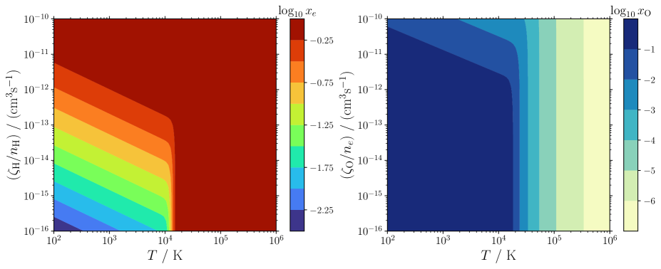
Figure 1: Contour plots for the ionized fraction of hydrogen (left) and neutral fraction of oxygen (right), as functions of $(T/{\rm\,K})$ and $(\zeta_{\mathrm{O}}/n_{\mathrm{H}})/\left({\rm\,cm}^{3}~{}\mathrm{s}^{-1}\right)$ (§3.2).

3.3 Is a higher neutral fraction possible?

From Figure 1, one can infer that the only hope of obtaining significant fractions of neutral oxygen is to stand on the lower-left corner, i.e. with low temperatures ($T$) and weak ionization-electron ratio ($\zeta_{\mathrm{O}}/n_{e}$). However, attempts in this domain will inevitably bog down to the following multilemma.

One way to lower $\zeta_{\mathrm{O}}/n_{e}$ is to have small $\zeta_{\mathrm{O}}$, which means either small $L_{\rm X}$ or strong attenuation of X-ray. Both possibilities will inhibit photoevaporative winds, as this wind launching mechanism requires intensive radiative heating. Another way to lower $\zeta_{\mathrm{O}}/n_{e}$ is to have greater $n_{e}$. Then here comes another problem: where do the electrons come from?

• If they come mainly from the photoionization of hydrogen (including secondary ionization by electrons or recombination photons in the X-ray ionization cascades), then the photon flux should be large enough to ionize oxygen to a greater extent–remember $\sigma_{\mathrm{O},i}$ is significantly greater than $\sigma_{\mathrm{H},i}$ for X-ray photons ($\sim 10^{4}$ times at $h\nu=1~{}{\rm\,keV}$), due to the interactions with inner shell electrons.

• If they are produced via collisional ionization, then the temperature should be high enough to significantly ionize hydrogen–this will also lead to significant ionization of oxygen, as their ionization energy values are almost the same.

All in all, in winds driven by photoevaporation, it is impossible to achieve desired thermochemical conditions, which are necessary to yield the observed luminosity of the [O i] $6300~{}\mathrm{\AA}$ emission within $R=1~{}\mathrm{AU}$.

4 Semi-analytic Constraints

The analyses in §2 focus on the energetics of the whole wind, without placing significant emphasis on the motion of the fluid itself. This approach may have a limitation: the localized injection of energy may not fully account for the changes in circumstances that occur when gases move outward. This section integrates mechanical and thermochemical equations with a global approach, guided by the typical geometry of disk photoevaporation depicted in Figure 4. The formulations of these equations are elaborated in Appendix C. It is worth noting that the complete set of physical processes involved in the photoionized gas exceeds the capabilities of analytic solutions. Therefore, if any simplifications need to be made, we choose to err on the side of caution.

4.1 Ionized Corona Solutions

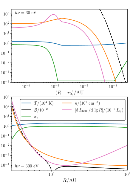
Figure 2: Example solutions for a bound model (upper panel; note that its horizontal axis is $R-r_{0}$) and an unbound model (lower panel), showing the hydrostatic and thermochemical profiles (distinguished by colors). The [O i] emissions are presented in the luminosity per logarithm radius. Both models have the same key parameters ($M_{*}=M_{\odot}$, $r_{0}=0.3~{}\mathrm{AU}$, $n_{0}=10^{9}~{}{\rm\,cm}^{-3}$, $L_{\rm XUV}=10^{-3}\;L_{\odot}$), with one exception: the bound model has XUV photon energy $h\nu=30~{}{\rm\,eV}$, while the unbound model has $h\nu=300~{}{\rm\,eV}$. The Bernoulli parameters (Appendix C.2) are presented in dashed lines when negative and in solid lines when positive.

Two solutions with typical selections of physical parameters are presented in Figure 2 showing an unbound solution with XUV (X-ray and extreme ultraviolet) photon energy $h\nu=300~{}{\rm\,eV}$, and a bound solution with $h\nu=30~{}{\rm\,eV}$. The unbound model exhibits a sign transition in the Bernoulli parameter $\mathcal{B}$ at $R\sim 1~{}\mathrm{AU}$ (eq. C7), at which the mass density already drops by a factor $\lesssim 10^{-5}$ compared to $n_{0}$. The sound speed at that location, corresponding to the temperature $T\sim 2\times 10^{4}~{}{\rm\,K}$, is around $\sim 12~{}{\rm\,km}~{}\mathrm{s}^{-1}$, yet the low mass density leads to a negligible mass-loss rate $\dot{M}\lesssim 10^{-12}~{}M_{\odot}~{}\mathrm{yr}^{-1}$. The other model is bound because the energy injection by the $h\nu=30~{}{\rm\,eV}$ photons is insufficient for the gas to escape. For both models, we also calculate the radial distribution of [O i] $6300~{}\mathrm{\AA}$ emissions via calculating the neutral fraction of oxygen (eq. 20). Both models have most of their [O i] emission concentrated near the center ($r\lesssim 0.5~{}\mathrm{AU}$), and the unbound model appears to be able to yield sufficient [O i] emission within the $R\lesssim 1~{}\mathrm{AU}$ spatial range ($\sim 10^{-5}\;L_{\odot}$ for the unbound model, and $\sim 10^{-6}\;L_{\odot}$ for the bound model). Nevertheless, their mass-loss rates are tiny or even vanishing, with our simplifications over-estimating the $\dot{M}$. Such low $\dot{M}$ values make the physical scenario drastically different from Owen et al. (2010, 2012); Ercolano & Owen (2016); Rab et al. (2023). This contradiction clearly indicates that the proper mechanism explaining adequate disk dispersal with proper [O i] emission can not rely solely on photoevaporation.

4.2 The Dilemma: Outflow versus Luminosity

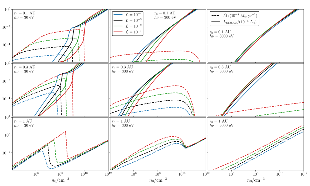
Figure 3: Photoevaporative mass-loss rates ($\dot{M}$) and [O i] $6300~{}\mathrm{\AA}$ luminosities within $R<1~{}\mathrm{AU}$ ($L_{\rm 6300,AU}$) with different physical parameters: inner boundary radius $r_{0}$, inner boundary hydrogen nuclei number density $n_{0}$, XUV luminosity $\mathcal{L}\equiv L_{\rm XUV}/L_{\odot}$, and XUV photon energy $h\nu$. Different $\mathcal{L}$ are distinguished by colors in each panel as noted; different line shapes show different physical quantities: dashed lines for $\dot{M}/(10^{-8}~{}M_{\odot}~{}\mathrm{yr}^{-1})$, and solid lines for $L_{\rm 6300,AU}/(10^{-5}~{}L_{\odot})$. Various selections of inner radius $r_{0}$ and XUV photon energy $h\nu$ are presented in different panels. Note that $L_{6300,\mathrm{AU}}$ vanishes for models with $r_{0}=1~{}\mathrm{AU}$.

Other possible values of physical parameter are explored in Figure 3, showing the mass-loss rates ($\dot{M}$) and the [O i] luminosities within the innermost $1~{}\mathrm{AU}$ ($L_{6300,\mathrm{AU}}$) for various XUV luminosities, XUV photon energies, and the radii and the mass densities at the inner radial boundaries. Figure 3 reveals that almost all models with $n_{0}<10^{10}~{}{\rm\,cm}^{-3}$ give insufficient mass-loss rates even with excessive, unphysical XUV luminosities (up to $10^{-1}~{}L_{\odot}$). In fact, such a high density ($n_{0}\sim 10^{10}~{}{\rm\,cm}^{-3}$) at the wind base is very unlikely. Lifting dense gas to the disk surface requires significant heating below the disk surfaces, which is almost impossible due to the photoevaporative wind geometry. In addition, for $h\nu\gtrsim 300~{}{\rm\,eV}$ photons, the coronal gas near $r_{0}$ is predominantly neutral (e.g., Figure 2), and excessively high $n_{0}$ will cause considerable absorption at $r\gtrsim 0.3~{}\mathrm{AU}$ (see also eq. 7). Numerical simulations have also confirmed that the wind should never be so dense (e.g. Wang & Goodman, 2017). Even when the wind is driven by the non-ideal magnetohydrodynamic mechanisms and is relatively slow and dense, the wind-base density is still typically $n_{0}\lesssim 10^{8}~{}{\rm\,cm}^{-3}$ (e.g. Bai 2017; Wang et al. 2019). Therefore, the gas should never be as dense as $n_{0}\gtrsim 10^{10}~{}{\rm\,cm}^{-3}$ at the beginning of the flux tube in the disk corona or even near the disk surface, and the mass-loss rates should be insufficient (i.e., $\ll 10^{-8}~{}M_{\odot}~{}\mathrm{yr}^{-1}$) in the first place. Such results are also consistent with the estimations in §2.1.

One may notice a dilemma emerging from the models presented in Figure 3: a photoevaporative disk cannot produce sufficient [O i] emissions within $\sim 1~{}\mathrm{AU}$ while maintaining adequate mass-loss rates. The models with $r_{0}=1~{}\mathrm{AU}$ and $h\nu\gtrsim 300{\rm\,eV}$ seem to resolve such a dilemma, yet Fang et al. (2023b) have already indicated that the [O i] emission is concentrated within the innermost sub-au region. Such a dilemma confirms the arguments in §2, §3, and especially §3.3. Photoionization must make its choice between the energy injection and the neutral fraction: an unbound model with adequate mass-loss rates always has high ionized fractions and low emissivities from neutral oxygen, and vice versa. It is worth noting that these models have underestimated the cooling processes. Incorporating these complexities will further bound the gas or reduce the mass-loss rates, confirming the dilemma with higher confidence.

5 Discussion and Summary

After calculating the conditions required by the observed [O i] $6300~{}\mathrm{\AA}$ emission, this letter concludes that X-ray photoevaporation can not be the proper mechanism of PPD wind launching from the innermost sub-au regions. X-ray alone provides insufficient heating for wind launching, which is further restricted by cooling mechanisms, especially the dust-gas thermal accommodation. Even if a wind is launched, the temperatures as well as the X-ray photoionization required to unbind the gas from the star gravitationally will also destruct neutral oxygen atoms overwhelmingly.

One may find it curious that, with all the arguments presented in this section, why in the first place were the winds “launched” in some previous works, such as R23 and Ercolano & Owen (2016)? The biggest issue is the detachment of thermodynamics from hydrodynamics, using a simple mapping of gas temperature $T$ onto the ionization parameter $\xi\equiv F_{X}/n_{\mathrm{H}}$ (Owen et al., 2010). This is, nevertheless, an inconsistent way of dealing with the co-evolution of thermochemistry and hydrodynamics. Significant heating almost stops due to the lack of neutral materials inside the photoionized wind. Meanwhile, the adiabatic expansion due to outward motion will cause a drop in gas temperature. Quantifying these processes with a simple $\xi$ will lead to unrealistic outcomes.

Analyses of scalings are helpful in revealing the underlying physics. When a wind fluid element is sufficiently far away from the wind base, its density scales as $n\propto r^{-2}$, where $r$ is its radial location. At that place, the unattenuated radiation flux also scales as $F\propto r^{-2}$. These scalings yield $\xi\equiv F/n\propto r^{0}$, i.e. the ionization parameter is insensitive to the distance. The $\xi-T$ mapping technique thus yields largely constant temperature in the winds. According to the Parker wind theory, systems with an adiabatic index $\gamma\equiv\mathrm{d}\ln P/\mathrm{d}\ln\rho<3/2$ always launch winds, let alone this roughly isothermal condition (Parker, 1958; Meyer-Vernet, 2007). Consequently, the $\xi-T$ mapping scheme, by effectively setting $\gamma\simeq 1$, leads to a scenario in which the winds will always be launched no matter what photon energy or luminosity one uses. This is unrealistic, as in reality, there should be no winds when the photon energy is too low or when the luminosity is insufficient. Even when the system manages to achieve constant temperature, the physical parameters required to launch winds with $\sim 10^{-9}~{}M_{\odot}~{}\mathrm{yr}^{-1}$ mass-loss rates are still mostly unphysical from the $R\lesssim 0.3~{}\mathrm{AU}$ part of the disk (see also §2.1, §4.2).

Another consideration can help us quantify the severity of the mistake that the $\xi-T$ mapping makes. When converting thermal energy to mechanical energy, the Carnot theorem gives the upper limit of efficiency,

$$\eta<1-\frac{T_{\rm low}}{T_{\rm high}},$$ (21)

where $T_{\rm low}$ and $T_{\rm high}$ are the low-end and high-end of the mechanism. To escape from $R=0.3~{}\mathrm{AU}$, we can take $T_{\rm high}\sim 6\times 10^{4}~{}{\rm\,K}$. When the gas expands towards the vacuum, as a disk wind eventually does, $T_{\rm low}\ll T_{\rm high}$, and thus $\eta\sim 1$. The disk wind system converts the thermal energy into mechanical energy with high efficiencies. The $\xi-T$ mapping approach, in contrast, maintains largely invariant gas temperature while increasing the mechanical energy of the system until it’s roughly equivalent to the gas thermal energy. In such an approach, the total radiation-injected energy is actually double-counted, leading to unrealistic consequences.

In addition, the $\xi-T$ mapping cannot properly represent the cooling processes. Most radiative coolings are two-body processes, with $\Lambda\propto n^{2}$, a totally different scaling from a simple $\xi$. On the other hand, higher density results in stronger recombination and attenuation of the photodissociation and photoionization radiation fluxes, which could potentially destroy the coolants and limit the cooling. The density and radiation flux intensity undergo drastical variation near the wind base, and therefore require detailed treatments to the cooling processes.

In conclusion, consistent co-evolution of non-equilibrium thermochemistry and dynamics (hydrodynamics and MHD) is a necessity in physically modeling the outflows of PPDs and plausibly explain the observed features of disk wind indicators.

Y. Lin and L. Wang acknowledge the computing resources provided by the Kavli Institute for Astronomy and Astrophysics in Peking University. We thank our collegues for helpful discussions: Gregory Herczeg, Xiao Hu, Haifeng Yang, Xinyu Zheng.

Appendix A Mean free path of particles and hydrodynamics

One should prove that the hydrodynamics is applicable to the problem, and the escape of atoms as particles should not be relevant, to justify the arguments based on hydrodynamics. Even if a fraction of gas particles are sufficiently energetic to escape, the mean-free-path of these particles can be estimated (the subscripts “nn”, “nc”, and “cc” indicate neutral-neutral, neutral-charged, and charged-charged collisions, and $r_{\rm n}$ is the size of the neutral particles; see also Draine 2011),

$$\begin{split}&\lambda_{\rm nn}\simeq 5\times 10^{-6}~{}\mathrm{AU}\times\left(\frac{n}{10^{7}~{}{\rm\,cm}^{-3}}\right)^{-1}\left(\dfrac{r_{\rm n}}{\mathrm{\AA}}\right)^{-2},\\ &\lambda_{\rm nc}\lesssim 5\times 10^{-7}~{}\mathrm{AU}\times\left(\frac{n}{10^{7}~{}{\rm\,cm}^{-3}}\right)^{-1},\\ &\lambda_{\rm cc}\simeq 3\times 10^{-9}~{}\mathrm{AU}\times\left(\frac{T}{10^{4}~{}{\rm\,K}}\right)^{2}\left(\frac{n_{e}}{10^{7}~{}{\rm\,cm}^{-3}}\right)^{-1}.\end{split}$$ (A1)

These lengths are tiny compared to the physical scales, which disable the physical picture that the “high-energy tail” of the Maxwell distribution could escape, and assure the applicability of hydrodynamics.

Appendix B The Impact of X-ray on Dust Temperatures

Is the assumption that “$T_{\rm dust}$ is unaffected by the X-ray irradiation” reasonable? We note that the dust grains without irradiaion are in thermodynamic equilibria with the diffuse infrared radiation (originating from the central star) within the disk (Chiang & Goldreich, 1997). For dust grain sizes no smaller than the infrared wavelengths, the Stefan-Boltzmann law constraints the deviation from the equilibrium temperature, leading to the following estimates of the timescale that dust temperatures converges to the equilibrium temperature $T_{\rm dust,0}$ (the subscript “sb” is for the Stefan-Boltzmann law):

$$\begin{split}\lambda_{\rm sb}&\sim 4\pi a_{\rm dust}^{2}\sigma_{B}(T_{\rm dust}^{4}-T_{\rm dust,0}^{4})\\ &\sim 0.5~{}{\rm\,erg}~{}\mathrm{s}^{-1}\times\left(\frac{a_{\rm dust}}{1~{}{\rm\,\mu m}}\right)^{2}\\ &\quad\times\left(\frac{T_{\rm dust,0}}{511~{}{\rm\,K}}\right)^{4}\left[\left(\frac{T_{\rm dust,0}}{T_{\rm dust}}\right)^{4}-1\right].\end{split}$$ (B1)

The maximum amount of heating that this dust grain is “responsible of” can be estimated by,

$$\begin{split}\gamma_{\rm dust}&\sim\left(\frac{\pi a_{\rm dust}^{2}}{\sigma_{\rm dust}/\mathrm{H}}\right)\gamma_{\rm X}\\ &\sim 3\times 10^{13}\gamma_{\rm X}\ \left(\frac{a_{\rm dust}}{{\rm\,\mu m}}\right)^{2}\left(\frac{\sigma_{\rm dust}/\mathrm{H}}{10^{-21}~{}{\rm\,cm}^{2}}\right)^{-1}.\end{split}$$ (B2)

The factor $3\times 10^{13}$ may seem a tremendous number. However, the product with $\gamma_{\rm X}$ is still dwarfed by the $\lambda_{\rm sb}$, which can eventually cause a temperature raise by $(T_{\rm dust,0}-T_{\rm dust})\sim 3\times 10^{-3}~{}{\rm\,K}$. When we consider smaller dust grains, the stiffer dependence of dust emissivity on temperature (roughly $\propto T^{6}$, see also §22 in Draine 2011). In other words, due to the stiff thermal balance between dusts and diffuse radiation fields in the disks, $T_{\rm dust}$ is not raised by the X-ray irradiation.

Appendix C Semi-analytic Solutions of the Irradiated Disk Corona

C.1 Formulations of the Coronal hydrostatic

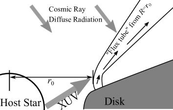
Figure 4: Schematic setups for the semi-analytic models (§4), showing an XUV irradiated “flux tube” originating from $R=r_{0}$.

When there are no outflows, hydrostatic models properly describe the structures of the heated disk corona. Even with outflows, fluids are still in hydrostatic below the wind base. Figure 4 illustrates that the fluid geometry can be described by fluid “flux tubes”, which have approximately the same solid angle at different radii, for both the static fluids stalled above a point of the disk surface, and the wind launched from a point on the disk. The guiding equations can be written for the hydrostatic with thermochemistry and radiation in one dimension in spherical geometry,

$$\begin{split}&0=\partial_{R}p+\frac{GM_{*}m_{\mathrm{H}}n}{R^{2}}\ ,\\ &p=n(1+x_{e})k_{\rm B}T\ ,\\ &0=\alpha_{\mathrm{H}}x_{e}^{2}-\frac{F\sigma_{\mathrm{H},i}}{n}(1-x_{e})-k_{\rm H,ci}x_{e}(1-x_{e})\ ,\\ &0=\frac{F\sigma_{\mathrm{H},i}}{n}(1-x_{e})(h\nu-I_{\mathrm{H}})-\Lambda\ ,\\ &0=\partial_{R}\ln F+\left[\frac{2}{R}+n\sigma_{\mathrm{H},i}(1-x_{e})\right].\end{split}$$ (C1)

Here, $M_{*}$ is the mass of the host star, and $F$ is the photon number flux of the XUV photons. Eqs. (C1) are solved in their dimensionless forms with the following dimensionless transforms (where we use $n_{0}\equiv 1/(\sigma_{\rm pi}r_{0})$ for the reference number density, and $k_{0}\equiv 10^{-8}~{}{\rm\,cm}^{3}~{}\mathrm{s}^{-1}$ for the fiducial rate coefficient),

$$\begin{split}&\zeta\equiv\frac{R}{r_{0}},\ \varrho\equiv\frac{n}{n_{0}},\ \varpi\equiv\frac{pr_{0}}{GM_{*}m_{\mathrm{H}}n_{0}},\ \Theta\equiv\frac{k_{\rm B}T}{I_{\mathrm{H}}},\\ &\varphi\equiv\frac{F\sigma_{\mathrm{H},i}}{n_{0}k_{0}},\ \epsilon\equiv\frac{h\nu}{I_{\mathrm{H}}},\ \Gamma\equiv\frac{I_{\mathrm{H}}r_{0}}{GM_{*}m_{\mathrm{H}}}.\end{split}$$ (C2)

The collisional ionization and recombination rates are reduced to dimensionless functions (see also eqs. 18),

$$\begin{split}&k_{\rm H,ci}\equiv k_{0}\kappa(\Theta)\ ,\ \kappa(\Theta)\simeq 2.3\ \Theta^{1/2}\mathrm{e}^{-1/\Theta}\ ;\\ &\alpha_{\mathrm{H}}\equiv k_{0}A(\Theta)\ ,\ A(\Theta)\simeq 3.2\times 10^{-6}\ \Theta^{-0.75}\ .\end{split}$$ (C3)

The cooling term is decomposed into three components: collisional ionization cooling ($\Lambda_{\rm ci}$), recombination cooling ($\Lambda_{\rm rec}$), and Lyman $\alpha$ cooling ($\Lambda_{\text{Ly}\alpha}$). These terms are also reduced into their dimensionless forms (see also Draine 2011, Murray-Clay et al. 2009),

$$\begin{split}\Lambda_{\rm rec}&\equiv\lambda_{\rm rec}(\Theta)x_{e}^{2}\times I_{\mathrm{H}}k_{0}\ ,\\ \Lambda_{\text{Ly}\alpha}&=\lambda_{\text{Ly}\alpha}(\Theta)x_{e}(1-x_{e})\times I_{\mathrm{H}}k_{0}\ ,\\ \Lambda_{\rm ci}&=\kappa(\Theta)x_{e}(1-x_{e})\times I_{\mathrm{H}}k_{0}\ ;\\ \lambda_{\text{Ly}\alpha}(\Theta)&\simeq\frac{3.44}{1+1.26\Theta^{1/2}}\exp\left(-\frac{3}{4\Theta}\right)\ ,\\ \lambda_{\rm rec}(\Theta)&\simeq(0.569-0.0416\ln\Theta)\;\Theta\;A(\Theta)\ .\end{split}$$ (C4)

The total cooling is decomposed into $\Lambda=\Lambda_{\rm ci}+\Lambda_{\rm rec}+\beta\Lambda_{\text{Ly}\alpha}$, where the $\beta$ factor is the escape probability of cooling Ly$\alpha$ photons. It is also noted that the set of cooling processes involved is far from being complete. By setting a default $\beta\rightarrow 0$ and ignoring all other cooling processes, the gases become less bound, making them easier to escape and putting us on the safe side by exaggerating the effect oppositing to our conclusions.

With such transforms, the dimensional eqs. (C1) are recast into the dimensionless form,

$$\begin{split}\partial_{\zeta}\varphi&=-[2\zeta^{-1}+\varrho(1-x_{e})]\varphi\ ,\\ \partial_{\zeta}\varpi&=-\zeta^{-2}\varrho\ ,\\ 0&=\varphi\varrho^{-1}(1-x_{e})+\kappa(\Theta)x_{e}(1-x_{e})-A(\Theta)x_{e}^{2}\ ,\\ 0&=\varphi\varrho^{-1}(1-x_{e})(\epsilon-1)-\lambda_{\rm rec}(\Theta)x_{e}^{2}\\ &\qquad-[\kappa(\Theta)+\beta\lambda_{\text{Ly}\alpha}(\Theta)]x_{e}(1-x_{e})\ ,\\ \varpi&=\Gamma(1+x_{e})\varrho\Theta\ .\end{split}$$ (C5)

Two extra constraints are desired when solving the algebraic part of these equations. First, the carbon element should be predominantly ionized by the FUV photons (with $h\nu>11.2~{}{\rm\,eV}$) from the central star and the diffuse interstellar radiation fields. A lower bound $x_{e,\mathrm{min}}=X_{\mathrm{C}}$ should be imposed, and we choose $X_{\mathrm{C}}=1.4\times 10^{-4}$. Second, the optical and infrared radiation from the host star also imposes a lower limit on the gas temperature,

$$T_{\mathrm{min}}\simeq T_{\rm eq}=886~{}{\rm\,K}\times\left(\dfrac{L_{*}}{L_{\odot}}\right)^{1/4}\left(\dfrac{R}{0.1~{}\mathrm{AU}}\right)^{-1/2}.$$ (C6)

Here $T_{\rm eq}$ is the equilibrium temperature of black bodies. We choose the bolometric luminosity $L_{*}=L_{\odot}$ in this work, and determine the lower bound for $T$ (and for $\Theta$ subsequently) according to the distance to the star. Meanwhile, the ionization by cosmic ray can also be non-negligible when the density is sufficiently low, and we include an extra $\zeta_{\rm CR}=10^{-17}~{}\mathrm{s}^{-1}$ as another ionization source in addition to the central star irradiation.

C.2 Properties of the Solutions

The eqs. (C5) can be solved with semi-analytic methods by selecting a set of physical parameters and inner boundary conditions at $r_{0}$. The solutions can be roughly categorized into three types:

• Gravitationally bound. When the injected irradiation has tiny thermochemical impacts, the situation is similar to an externally gravitated polytrope: all gases are gravitationally bound and yield no outflows, the system will have a surface (at which the gas density and pressure vanish) at a finite radius.

• Pressure bound. When the gas pressure converges to a constant values (“terminal pressure”) at infinite distances (similar to isothermal atmospheres gravitated by the central star), and such constant value is lower than the ISM pressure ($\sim 4\times 10^{-13}~{}{\rm dyn~{}cm}^{-2}$ for both warm and cool neutral media; see Draine 2011).

• Unbound. When the terminal pressure is greater than the surroundings.

In the unbound case, one should in principle connect a steady-state hydrodynamic solution to a hydrostatic solution at a specific point (often called “wind base”). Nevertheless, such problems are always underdefinite when connecting a hydrostatic solution to hydrodynamic solutions analytically (e.g. Wang & Dai, 2018), and the hydrodynamic part is always numerically stiff and less trustworthy. Therefore, we estimate the most important parameter for outflows–the mass-loss rates–by $\dot{M}=4\pi r_{s}^{2}c_{s}\rho_{s}$, in which $r_{s}$, $c_{s}$, and $\rho_{s}$ are the radius, sound speed, and mass density at the sonic critical radius where the radial outflow becomes supersonic. Since the actual mass density at the critical radius is certainly less than the hydrostatic estimation because of gas acceleration, this simplification is over-estimating the mass-loss. Such $\dot{M}$ is an extrapolation of a flux tube to the full $4\pi$ solid angle, which also lead to an over-estimation due to the geometry (see also Figure 4).

For a perfectly isothermal Parker wind (Parker, 1958), $r_{s}$ is located at $r_{s}=GM_{*}/2c_{s}^{2}$. The models described by eqs. (C5) have variable temperatures. We thus define a dimensionless Bernoulli parameter,

$$\mathcal{B}\equiv\gamma\varpi/(\gamma-1)-\varrho/\zeta$$ (C7)

here $\gamma$ is the adiabatic index and $\gamma=5/3$ in all relevant cases in this work. When a solution is gravitationally bound, its $\mathcal{B}$ is always negative. The unbound solutions, in contrast, have transition points from negative $\mathcal{B}$ to positive $\mathcal{B}$, and we approximate the sonic critical point and associated physical quantities by this transition. Note that there are also cases whose $\mathcal{B}$ becomes positive but pressure converges to very low values at large radii.

References

- Alexander (2008) Alexander, R. D. 2008, MNRAS, 391, L64
- Alexander et al. (2006a) Alexander, R. D., Clarke, C. J., & Pringle, J. E. 2006a, MNRAS, 369, 216
- Alexander et al. (2006b) —. 2006b, MNRAS, 369, 229
- Bai (2017) Bai, X.-N. 2017, ApJ, 845, 75
- Bai & Goodman (2009) Bai, X.-N., & Goodman, J. 2009, ApJ, 701, 737
- Bai et al. (2016) Bai, X.-N., Ye, J., Goodman, J., & Yuan, F. 2016, ApJ, 818, 152
- Banzatti et al. (2019) Banzatti, A., Pascucci, I., Edwards, S., et al. 2019, ApJ, 870, 76
- Chiang & Goldreich (1997) Chiang, E. I., & Goldreich, P. 1997, ApJ, 490, 368
- Draine (2011) Draine, B. T. 2011, Physics of the Interstellar and Intergalactic Medium (Princeton University Press)
- Ercolano & Owen (2016) Ercolano, B., & Owen, J. E. 2016, MNRAS, 460, 3472
- Fang et al. (2023a) Fang, M., Pascucci, I., Edwards, S., et al. 2023a, ApJ, 945, 112
- Fang et al. (2023b) Fang, M., Wang, L., Herczeg, G. J., et al. 2023b, Nature Astronomy, 7, 905
- Goldsmith (2001) Goldsmith, P. F. 2001, ApJ, 557, 736
- Gorti & Hollenbach (2009) Gorti, U., & Hollenbach, D. 2009, ApJ, 690, 1539
- Kramida et al. (2022) Kramida, A., Yu. Ralchenko, Reader, J., & and NIST ASD Team. 2022, National Institute of Standards and Technology, Gaithersburg, MD. https://physics.nist.gov/asd
- Meyer-Vernet (2007) Meyer-Vernet, N. 2007, Basics of the Solar Wind (Cambridge University Press, Cambridge)
- Murray-Clay et al. (2009) Murray-Clay, R. A., Chiang, E. I., & Murray, N. 2009, ApJ, 693, 23
- Nemer et al. (2020) Nemer, A., Goodman, J., & Wang, L. 2020, ApJ, 904, L27
- Owen et al. (2012) Owen, J. E., Clarke, C. J., & Ercolano, B. 2012, MNRAS, 422, 1880
- Owen et al. (2010) Owen, J. E., Ercolano, B., Clarke, C. J., & Alexander, R. D. 2010, MNRAS, 401, 1415
- Parker (1958) Parker, E. N. 1958, ApJ, 128, 664
- Pascucci et al. (2023) Pascucci, I., Cabrit, S., Edwards, S., et al. 2023, in Astronomical Society of the Pacific Conference Series, Vol. 534, Protostars and Planets VII, ed. S. Inutsuka, Y. Aikawa, T. Muto, K. Tomida, & M. Tamura, 567
- Rab et al. (2023) Rab, C., Weber, M. L., Picogna, G., Ercolano, B., & Owen, J. E. 2023, ApJ, 955, L11, (R23)
- Wang et al. (2019) Wang, L., Bai, X.-N., & Goodman, J. 2019, ApJ, 874, 90
- Wang & Dai (2018) Wang, L., & Dai, F. 2018, ApJ, 860, 175
- Wang & Goodman (2017) Wang, L., & Goodman, J. 2017, ApJ, 847, 11
- Wardle & Königl (1993) Wardle, M., & Königl, A. 1993, ApJ, 410, 218
- Xu & Bai (2016) Xu, R., & Bai, X.-N. 2016, ApJ, 819, 68