Off-diagonal estimates of partial Bergman kernels on $S^{1}$-symmetric Kรคhler manifolds

Ood Shabtai shabtai@imj-prg.fr
Partially supported by the DFG funded project SFB/TRR 191 (Project-ID 281071066-TRR 191), and the ANR-DFG project QuaSiDy (Project-ID ANR-21-CE40-0016).
Abstract

We establish local asymptotic estimates of partial Bergman kernels on closed, $S^{1}$-symmetric Kรคhler manifolds. The main result concerns the scaling asymptotics of partial Bergman kernels at generic off-diagonal points in which they are not negligible. The case of the two-dimensional sphere is discussed in detail.

1 Introduction

Let $(M,\omega)$ be a connected closed Kรคhler manifold of complex dimension $n$. Assume that $L\to M$ is a holomorphic Hermitian line bundle such that the curvature of its Chern connection equals $-i\omega$. The space of holomorphic sections of $L^{\otimes k}$ is a finite-dimensional complex vector space $\mathcal{H}_{k}$, equipped with a natural inner product $\langle\cdot,\cdot\rangle$. The latter is obtained by integrating the fiberwise Hermitian product of $L^{\otimes k}$ with respect to the Liouville measure $\mu=\frac{\lvert\omega^{\wedge n}\rvert}{n!}$.

Assume that $\varphi:S^{1}\times M\to M$ is a holomorphic Hamiltonian $S^{1}$-action. Thus, there exists a smooth function $H:M\to\mathbb{R}$ such that $\varphi$ is the flow of its Hamiltonian vector field $X_{H}$. The โ€quantum counterpartโ€ of $H$ is the Hermitian operator $\hat{H}_{k}\in\operatorname{End}(\mathcal{H}_{k})$ specified by111Since $X_{H}$ generates a holomorphic circle action, $\hat{H}_{k}$ preserves holomorphic sections.

$$\hat{H}_{k}=\mathcal{M}_{H}-\frac{i}{k}\nabla^{\otimes k}_{X_{H}},$$

where $\nabla:C^{\infty}(M,L)\to C^{\infty}(M,T^{*}M\otimes L)$ is the Chern connection, and $\mathcal{M}_{H}$ is the operator of multiplication by $H$.

Fix a regular value $E\in H(M)$, and consider the spectral projection

ฮ k,E=๐Ÿ™[E,โˆž)โ€‹(H^k).subscriptฮ ๐‘˜๐ธsubscript1๐ธsubscript^๐ป๐‘˜\Pi_{k,E}=\mathbbm{1}_{[E,\infty)}(\hat{H}_{k}).

The Schwartz kernel of ฮ k,Esubscriptฮ ๐‘˜๐ธ\Pi_{k,E}, which we also denote by ฮ k,Esubscriptฮ ๐‘˜๐ธ\Pi_{k,E} (by an abuse of notation), is termed a partial Bergman kernel222The projection ฮ k,Esubscriptฮ ๐‘˜๐ธ\Pi_{k,E} is a spectral projection, hence the partial Bergman kernel ฮ k,Esubscriptฮ ๐‘˜๐ธ\Pi_{k,E} is sometimes called a spectral partial Bergman kernel. ([27, 28, 1, 7, 21, 22, 9, 10]). This terminology references the โ€fullโ€ Bergman kernel, which is the Schwartz kernel of the orthogonal projection ฮ k:L2โ€‹(M,LโŠ—k)โ†’โ„‹k:subscriptฮ ๐‘˜โ†’superscript๐ฟ2๐‘€superscript๐ฟtensor-productabsent๐‘˜subscriptโ„‹๐‘˜\Pi_{k}:L^{2}(M,L^{\otimes k})\to\mathcal{H}_{k}. The main goal of the present article is to study the asymptotic behaviour of the partial Bergman kernel ฮ k,Esubscriptฮ ๐‘˜๐ธ\Pi_{k,E} as $k\to\infty$. We focus on the behaviour away from the diagonal $\Delta_{M}\subset M\times M$, since the asymptotic properties of ฮ k,Esubscriptฮ ๐‘˜๐ธ\Pi_{k,E} on $\Delta_{M}$ are already understood quite well. Specifically, it is shown (among other things) in [27, 28] that

ฮ k,Eโ€‹(z,z)={ฮ kโ€‹(z,z)+๐’ชโ€‹(kโˆ’โˆž)ifย โ€‹Hโ€‹(z)>E,ฮ kโ€‹(z,z)โ€‹(12+๐’ชโ€‹(kโˆ’12))ifย โ€‹Hโ€‹(z)=E,๐’ชโ€‹(kโˆ’โˆž)ifย โ€‹Hโ€‹(z)<E.subscriptฮ ๐‘˜๐ธ๐‘ง๐‘งcasessubscriptฮ ๐‘˜๐‘ง๐‘ง๐’ชsuperscript๐‘˜ifย ๐ป๐‘ง๐ธsubscriptฮ ๐‘˜๐‘ง๐‘ง12๐’ชsuperscript๐‘˜12ifย ๐ป๐‘ง๐ธ๐’ชsuperscript๐‘˜ifย ๐ป๐‘ง๐ธ\Pi_{k,E}(z,z)=\left\{\begin{array}[]{ll}\Pi_{k}(z,z)+\mathcal{O}(k^{-\infty})&\text{if }H(z)>E,\\ \Pi_{k}(z,z)(\frac{1}{2}+\mathcal{O}(k^{-\frac{1}{2}}))&\text{if }H(z)=E,\\ \mathcal{O}(k^{-\infty})&\text{if }H(z)<E.\end{array}\right. (1)

In this work, we formulate statements analogous to (1), but for ฮ k,Eโ€‹(z,w)subscriptฮ ๐‘˜๐ธ๐‘ง๐‘ค\Pi_{k,E}(z,w), where zโ‰ w๐‘ง๐‘คz\neq w. Notably, ฮ k,Esubscriptฮ ๐‘˜๐ธ\Pi_{k,E} will be shown to โ€concentrateโ€ about the set

$$\{(z,z)\ |\ H(z)\geq E\}\cup\{(z,\varphi(t,z))\ |\ H(z)=E,\ t\in S^{1}\}\subset M\times M.$$

It is instructive to compare this type of behaviour with that of the Bergman kernel ฮ ksubscriptฮ ๐‘˜\Pi_{k} (or more generally, the kernels of Toeplitz operators333That is, operators of the form ฮ kโ€‹โ„ณF:โ„‹kโ†’โ„‹k:subscriptฮ ๐‘˜subscriptโ„ณ๐นโ†’subscriptโ„‹๐‘˜subscriptโ„‹๐‘˜\Pi_{k}\mathcal{M}_{F}:\mathcal{H}_{k}\to\mathcal{H}_{k}, where $F\in C^{\infty}(M)$.). The latter โ€concenratesโ€ on $\Delta_{M}$, and additionally, it admits a full, uniform asymptotic expansion. We refer the reader to Sect. 6 for some further details in this context. The properties of ฮ ksubscriptฮ ๐‘˜\Pi_{k} have been studied thoroughly (e.g., [18, 3, 2, 8, 4, 26]), and have found many applications in various fields of mathematics; they also underlie the results presented here.

Perhaps most notably, Theorem 4 of [27] describes the leading-order scaling asymptotics of ฮ k,Eโ€‹(z,z)subscriptฮ ๐‘˜๐ธ๐‘ง๐‘ง\Pi_{k,E}(z,z) in a $\frac{C}{\sqrt{k}}$-neighborhood of $H^{-1}(E)$. The main result of the present paper (Theorem 1.6) addresses the leading-order scaling asymptotics of ฮ k,Esubscriptฮ ๐‘˜๐ธ\Pi_{k,E} away from the diagonal.

Finally, we refer the reader to [27] for a concise review of various properties of $S^{1}$-symmetric Kรคhler manifolds which are relevant in our context. There is some overlap between the present paper and [27]; however, to the best of our knowledge, the off-diagonal asymptotic behaviour of partial Bergman kernels corresponding to spectral projections of quantum observables has yet to be described in the research literature. A treatment of the on-diagonal asymptotic properties of partial Bergman kernels of the same type considered here, but without an assumption of $S^{1}$-symmetry, may be found in [28].

1.1 Main results

The local behaviour of ฮ k,Esubscriptฮ ๐‘˜๐ธ\Pi_{k,E} away from $H^{-1}(E)\times H^{-1}(E)$ is straightforward to derive (up to an error of order $\mathcal{O}(k^{-\infty})$) using existing tools from the theory of Toeplitz operators ([4]), and does not require the assumption that $M$ is equipped with a holomorphic Hamiltonian $S^{1}$-action. In order to formulate the statements concisely, we use the following terminology (see also Sect. 3).

Definition 1.1 ([4]).

We say that a sequence $A_{k}\in\operatorname{End}(\mathcal{H}_{k})$ is negligible at $(z,w)\in M\times M$ if there exists a neighborhood $\mathcal{N}\subset M\times M$ of $(z,w)$ such that

$$\sup_{\mathcal{N}}\left|A_{k}\right|=\mathcal{O}(k^{-\infty}).$$

Here (by an abuse of notation), AkโˆˆCโˆžโ€‹(Mร—M,LโŠ—kโŠ (Lโˆ—)โŠ—k)subscript๐ด๐‘˜superscript๐ถ๐‘€๐‘€โŠ superscript๐ฟtensor-productabsent๐‘˜superscriptsuperscript๐ฟtensor-productabsent๐‘˜A_{k}\in C^{\infty}\left(M\times M,L^{\otimes k}\boxtimes(L^{*})^{\otimes k}\right) denotes the Schwartz kernel of $A_{k}\in\operatorname{End}(\mathcal{H}_{k})$, and its point-wise norm is defined using the Hermitian metric on LโŠ—kโŠ (Lโˆ—)โŠ—kโŠ superscript๐ฟtensor-productabsent๐‘˜superscriptsuperscript๐ฟtensor-productabsent๐‘˜L^{\otimes k}\boxtimes(L^{*})^{\otimes k} which is induced from that of $L$.

Theorem 1.2.

Let $F\in C^{\infty}(M)$, and denote F^k=ฮ kโ€‹(โ„ณFโˆ’ikโ€‹โˆ‡XFโŠ—k)โ€‹ฮ ksubscript^๐น๐‘˜subscriptฮ ๐‘˜subscriptโ„ณ๐น๐‘–๐‘˜subscriptsuperscriptโˆ‡tensor-productabsent๐‘˜subscript๐‘‹๐นsubscriptฮ ๐‘˜\hat{F}_{k}=\Pi_{k}\left(\mathcal{M}_{F}-\frac{i}{k}\nabla^{\otimes k}_{X_{F}}\right)\Pi_{k}. Fix $E\in\left[\min F,\max F\right]$, not necessarily a regular value. Let $z,w\in M$. There exists a neighborhood $\mathcal{N}\subset M\times M$ of $(z,w)$ such that the following holds.

  1. 1.

    If $F(z)>E$ or $F(w)>E$, then ๐Ÿ™[E,โˆž)โ€‹(F^k)โˆ’ฮ k=๐Ÿ™(โˆ’โˆž,E)โ€‹(F^k)subscript1๐ธsubscript^๐น๐‘˜subscriptฮ ๐‘˜subscript1๐ธsubscript^๐น๐‘˜\mathbbm{1}_{[E,\infty)}(\hat{F}_{k})-\Pi_{k}=\mathbbm{1}_{(-\infty,E)}(\hat{F}_{k}) is negligible at $(z,w)$.

  2. 2.

    If $F(z)<E$ or $F(w)<E$, then $\mathbbm{1}_{[E,\infty)}(\hat{F}_{k})$ is negligible at $(z,w)$.

Remark 1.3.

In particular, if zโ‰ w๐‘ง๐‘คz\neq w and $z\not\in F^{-1}(E)$ or $w\not\in F^{-1}(E)$, then $\mathbbm{1}_{[E,\infty)}(\hat{F}_{k})$ is negligible at $(z,w)$.

Remark 1.4.

In some cases (e.g., the settings of Lemma 4.6), the negligibility estimates provided by Theorem 1.2 can be improved, using suitable estimates of the Bergman kernel ([19]), to exponential decay estimates (cf. [27], Theorem 3). Similarly, in some cases (e.g., the settings of Corollary 4.9), exponential decay estimates are valid for Schwartz kernels of orthogonal projections onto single eigenspaces (cf. [27], Theorem 1).

We note that Theorem 1.2 implies that the ranges of spectral projections corresponding to disjoint classical domains are โ€orthogonal up to a negligible errorโ€. More precisely,

Corollary 1.5.

Let $F,G\in C^{\infty}(M)$. Assume that $E_{1}\in\left(\min F,\max F\right)$, that $E_{2}\in\left(\min G,\max G\right)$, and that $\{F\geq E_{1}\}\cap\{G\geq E_{2}\}=\emptyset$. Then

$$\|\mathbbm{1}_{[E_{1},\infty)}(\hat{F}_{k})\mathbbm{1}_{[E_{2},\infty)}(\hat{G}_{k})\|_{\operatorname{op}}=\mathcal{O}(k^{-\infty}).$$

Consequently, the algebras generated by the pairs $\mathbbm{1}_{[E_{1},\infty)}(\hat{F}_{k}),\ \mathbbm{1}_{[E_{2},\infty)}(\hat{G}_{k})$ are โ€asymptotically trivialโ€ (cf. [24]).

The main result of the present article describes the scaling asymptotics of ฮ k,Esubscriptฮ ๐‘˜๐ธ\Pi_{k,E} near $z_{0},w_{0}\in H^{-1}(E)$, z0โ‰ w0subscript๐‘ง0subscript๐‘ค0z_{0}\neq w_{0}. Throughout, we fix the normalization $\min H=0$ (note that $H$ is defined up to a constant). There exists $N\geq 1$ and an open dense subset $M_{N}\subset M$ such that for all $z\in M_{N}$, the stabilizer group of $z$ is the finite subgroup $S^{1}_{N}\subset S^{1}$ of order $N$. Accordingly, the spectrum of $\hat{H}_{k}$ equals444The case $N>1$ is reduced, in Lemma 4.4, to the case $N=1$, which is covered by [12]. $H(M)\cap\frac{N}{k}\mathbb{Z}$. Let $\{\psi_{a}\}_{a\in\mathbb{R}}$ denote the gradient flow of $H$, and $\varphi_{t}(z)=\varphi(t,z)$ (where $t\in S^{1}=\mathbb{R}/2\pi\mathbb{Z}$).

Theorem 1.6.

Let $\mathcal{O}_{z_{0}}\subset M$ denote the $S^{1}$-orbit of $z_{0}\in H^{-1}(E)$. Choose a local non-vanishing invariant section sinvsubscript๐‘ invs_{\operatorname{inv}} of $L$ in a neighborhood of $\mathcal{O}_{z_{0}}$. Denote

ฮ k,Eโ€‹(z,w)=๐’ฆk,Eโ€‹(z,w)โ€‹Skโ€‹(z,w),subscriptฮ ๐‘˜๐ธ๐‘ง๐‘คsubscript๐’ฆ๐‘˜๐ธ๐‘ง๐‘คsubscript๐‘†๐‘˜๐‘ง๐‘ค\Pi_{k,E}(z,w)=\mathcal{K}_{k,E}(z,w)S_{k}(z,w),

where $S_{k}(z,w)=\sigma^{\otimes k}(z)\otimes(\sigma^{*}(w))^{\otimes k}$, with ฯƒ=sinv|sinv|๐œŽsubscript๐‘ invsubscript๐‘ inv\sigma=\frac{s_{\operatorname{inv}}}{\lvert s_{\operatorname{inv}}\rvert}.

  1. 1.

    If $w_{0}\not\in\mathcal{O}_{z_{0}}$, then ฮ k,Esubscriptฮ ๐‘˜๐ธ\Pi_{k,E} is negligible at $(z_{0},w_{0})$.

  2. 2.

    If $z_{0}\in M_{N}$ and $t\in S^{1}$ satisfies ฯ†tโ€‹(z0)โ‰ z0subscript๐œ‘๐‘กsubscript๐‘ง0subscript๐‘ง0\varphi_{t}(z_{0})\neq z_{0}, then

    $$\left(\frac{2\pi}{k}\right)^{n}\mathcal{K}_{k,E}\left(\psi_{\frac{a}{\sqrt{k}}}(z_{0}),\psi_{\frac{b}{\sqrt{k}}}\circ\varphi_{t}(z_{0})\right)=\\ e^{-\frac{(a^{2}+b^{2})\|X_{H}(z_{0})\|^{2}}{2}}e^{-iN\lceil\frac{kE}{N}\rceil t}\frac{N\left(1-i\cot\left(\frac{Nt}{2}\right)\right)}{2\|X_{H}(z_{0})\|\sqrt{\pi k}}+C_{k}(a,b,t).$$

    Here,

    $$C_{k}(a,b,t)=\frac{C_{k,1}(a,b,t)}{k}+\frac{C_{k,2}(a,b,t)}{k^{\frac{3}{2}}},$$

    where $C_{k,1}(a,b,t)$, $C_{k,2}(a,b,t)$ satisfy that for any bounded $B\subset\mathbb{R}$ and closed interval $\mathcal{I}\subset S^{1}\setminus S^{1}_{N}$ there exist $c_{B,\mathcal{I},1},c_{B,\mathcal{I},2}>0$ such that

    $$|C_{k,1}(a,b,t)|\leq(|a|+|b|)c_{B,\mathcal{I},1},\ |C_{k,2}(a,b,t)|\leq c_{B,\mathcal{I},2}$$

    for all $a,b\in B,\ t\in\mathcal{I}$.

Let $V_{k}(t)=e^{ikt\hat{H}_{k}}$ denote the quantum evolution defined by $\hat{H}_{k}$. The proof of Theorem 1.6 is essentially an adaptation of the arguments used in [23]; it relies on basic methods from the theory of Fourier series, applied in the context of the unitary representation $V_{k}:S^{1}\to\operatorname{End}(\mathcal{H}_{k})$. A key role is played by the periodic Hilbert transform ([15]), which is a classical singular integral operator on $L^{2}(S^{1})$. We also use an estimate of the Schwartz kernels of projections onto single eigenspaces of $\hat{H}_{k}$ (the so-called equivariant Bergman kernels). The estimate is obtained by essentially the same method that was used in [27] to describe the on-diagonal scaling asymptotics of equivariant Bergman kernels.

Theorem 1.7.

Let $\lambda_{k}$ be an eigenvalue of $\hat{H}_{k}$ such that $\left|\lambda_{k}-E\right|=\mathcal{O}(k^{-1})$. Let ฮ k,ฮปkeqsubscriptsuperscriptฮ eq๐‘˜subscript๐œ†๐‘˜\Pi^{\operatorname{eq}}_{k,\lambda_{k}} be the orthogonal projection onto the corresponding eigenspace of $\hat{H}_{k}$. Fix $z_{0},w_{0}\in M$, and denote

ฮ k,ฮปkeqโ€‹(z,w)=๐’ฆk,ฮปkeqโ€‹(z,w)โ€‹Skโ€‹(z,w),superscriptsubscriptฮ ๐‘˜subscript๐œ†๐‘˜eq๐‘ง๐‘คsubscriptsuperscript๐’ฆeq๐‘˜subscript๐œ†๐‘˜๐‘ง๐‘คsubscript๐‘†๐‘˜๐‘ง๐‘ค\Pi_{k,\lambda_{k}}^{\operatorname{eq}}(z,w)=\mathcal{K}^{\operatorname{eq}}_{k,\lambda_{k}}(z,w)S_{k}(z,w),

where $S_{k}(z,w)$ is as specified in Theorem 1.6.

  1. 1.

    If Hโ€‹(z0)โ‰ E๐ปsubscript๐‘ง0๐ธH(z_{0})\neq E or Hโ€‹(w0)โ‰ E๐ปsubscript๐‘ค0๐ธH(w_{0})\neq E or $w_{0}\not\in\mathcal{O}_{z_{0}}$, then ฮ k,ฮปkeqsubscriptsuperscriptฮ eq๐‘˜subscript๐œ†๐‘˜\Pi^{\operatorname{eq}}_{k,\lambda_{k}} is negligible at $(z_{0},w_{0})$.

  2. 2.

    If $z_{0}\in M_{N}$, then

    $$\left(\frac{2\pi}{k}\right)^{n}\mathcal{K}^{\operatorname{eq}}_{k,\lambda_{k}}\left(\psi_{\frac{a}{\sqrt{k}}}(z_{0}),\psi_{\frac{b}{\sqrt{k}}}\circ\varphi_{t}(z_{0})\right)=\\ e^{-\frac{(a^{2}+b^{2})\|X_{H}(z_{0})\|^{2}}{2}}e^{-ik\lambda_{k}t}\frac{N}{\|X_{H}(z_{0})\|\sqrt{\pi k}}+C^{\operatorname{eq}}_{k}(a,b,t).$$

    Here,

    $$C^{\operatorname{eq}}_{k}(a,b,t)=\frac{C^{\operatorname{eq}}_{k,1}(a,b,t)}{k}+\frac{C^{\operatorname{eq}}_{k,2}(a,b,t)}{k^{\frac{3}{2}}},$$

    where $C^{\operatorname{eq}}_{k,1}(a,b,t)$, $C^{\operatorname{eq}}_{k,2}(a,b,t)$ satisfy that for any bounded $B\subset\mathbb{R}$ and closed interval $\mathcal{I}\subset S^{1}$ there exist $c^{\operatorname{eq}}_{B,\mathcal{I},1},c^{\operatorname{eq}}_{B,\mathcal{I},2}>0$ such that

    $$|C^{\operatorname{eq}}_{k,1}(a,b,t)|\leq(|a|+|b|)c^{\operatorname{eq}}_{B,\mathcal{I},1},\ |C^{\operatorname{eq}}_{k,2}(a,b,t)|\leq c^{\operatorname{eq}}_{B,\mathcal{I},2}$$

    for all $a,b\in B,\ t\in\mathcal{I}$.

2 Rotation of the two-dimensional sphere

In this section, we illustrate the results of Sect. 1.1 in the example of the action of $S^{1}$, by rotations, on the two-dimensional sphere. The latter is identified (via the stereographic projection from the north pole) with the complex projective line $\mathbb{C}P^{1}$ and equipped with the Fubini-Study form such that the total area equals $2\pi$. For conciseness, we focus on the case $N=1$, and $a=b=0$.

The Hamiltonian vector field of the function

$$H([z])=\frac{|z_{0}|^{2}}{|z_{0}|^{2}+|z_{1}|^{2}},\ z=(z_{0},z_{1})\in\mathbb{C}^{2}\setminus\{0\},$$

is specified (on {[z0:z1]โˆˆโ„‚P1|z1โ‰ 0}\{[z_{0}:z_{1}]\in\mathbb{C}P^{1}\ |\ z_{1}\neq 0\}) by

$$X_{H}([\zeta:1])=i\left(\zeta\partial_{\zeta}-\bar{\zeta}\partial_{\bar{\zeta}}\right),$$

and it generates the Hamiltonian flow

$$\varphi_{t}([z])=[U_{t}z],\ U_{t}=\left(\begin{array}[]{cc}e^{it}&0\\ 0&1\end{array}\right).$$

Clearly, $\varphi:S^{1}\times\mathbb{C}P^{1}\to\mathbb{C}P^{1}$ is a holomorphic circle action.

Remark 2.1.

On $S^{2}=\{x\in\mathbb{R}^{3}\ |\ |x|=1\}$, it holds that

$$H(x_{1},x_{2},x_{3})=\frac{1}{2}(x_{3}+1),$$

and $\varphi_{t}$ is the rotation by angle $t$ about the $x_{3}$ axis.

Let $L=\mathcal{O}(1)$ be the dual of the tautological line bundle on $\mathbb{C}P^{1}$. Then $L$ is a prequantum line bundle, and we let $\mathcal{H}_{k}=H^{0}(\mathbb{C}P^{1},L^{\otimes k})$ be the space of holomorphic sections of $L^{\otimes k}$. The quantum counterpart of $H$ is given by (5)

H^k=ฮ kโ€‹โ„ณHโˆ’12โ€‹kโ€‹ฮ”โ€‹Hโ€‹ฮ k,subscript^๐ป๐‘˜subscriptฮ ๐‘˜subscriptโ„ณ๐ป12๐‘˜ฮ”๐ปsubscriptฮ ๐‘˜\hat{H}_{k}=\Pi_{k}\mathcal{M}_{H-\frac{1}{2k}\Delta H}\Pi_{k},

and in our case, $\Delta H=-4H+2$, which means that

H^k=k+2kโ€‹ฮ kโ€‹โ„ณHโ€‹ฮ kโˆ’1kโ€‹Idโ„‹k.subscript^๐ป๐‘˜๐‘˜2๐‘˜subscriptฮ ๐‘˜subscriptโ„ณ๐ปsubscriptฮ ๐‘˜1๐‘˜subscriptIdsubscriptโ„‹๐‘˜\hat{H}_{k}=\frac{k+2}{k}\Pi_{k}\mathcal{M}_{H}\Pi_{k}-\frac{1}{k}\operatorname{Id}_{\mathcal{H}_{k}}.

As is common, we identify $\mathcal{H}_{k}$ with the space of bivariate homogeneous polynomials of degree $k$, denoted by $\mathbb{C}_{k}[z_{0},z_{1}]$, and equipped with a suitable inner product so that the set {sk,l|l=0,1,โ€ฆ,k}conditional-setsubscript๐‘ ๐‘˜๐‘™๐‘™01โ€ฆ๐‘˜\{s_{k,l}\ |\ l=0,1,...,k\}, where

sk,l=(k+1)โ€‹(kl)2โ€‹ฯ€โ€‹z0lโ€‹z1kโˆ’l,subscript๐‘ ๐‘˜๐‘™๐‘˜1binomial๐‘˜๐‘™2๐œ‹superscriptsubscript๐‘ง0๐‘™superscriptsubscript๐‘ง1๐‘˜๐‘™s_{k,l}=\sqrt{\frac{(k+1)\binom{k}{l}}{2\pi}}z_{0}^{l}z_{1}^{k-l}, (2)

forms an orthonormal basis of $\mathcal{H}_{k}$. In fact, this is an eigenbasis of $\hat{H}_{k}$ (cf. [16], Example 5.2.4), with

H^kโ€‹(sk,l)=ฮปk,lโ€‹sk,l,ฮปk,l=lk.formulae-sequencesubscript^๐ป๐‘˜subscript๐‘ ๐‘˜๐‘™subscript๐œ†๐‘˜๐‘™subscript๐‘ ๐‘˜๐‘™subscript๐œ†๐‘˜๐‘™๐‘™๐‘˜\hat{H}_{k}(s_{k,l})=\lambda_{k,l}s_{k,l},\ \lambda_{k,l}=\frac{l}{k}.

In particular, sinv=s1,0subscript๐‘ invsubscript๐‘ 10s_{\operatorname{inv}}=s_{1,0} is an invariant section of $L\to\mathbb{C}P^{1}$.

We can estimate the leading order of sk,lsubscript๐‘ ๐‘˜๐‘™s_{k,l} using only basic tools, as follows. Note that $H([z])=E$ if and only if $[z]=\left[\sqrt{\frac{E}{1-E}}e^{i\theta}:1\right]$ for some $\theta\in[0,2\pi]$.

Lemma 2.2.

As in Theorems 1.6, 1.7, consider the local normalized section ฯƒ=sinv|sinv|๐œŽsubscript๐‘ invsubscript๐‘ inv\sigma=\frac{s_{\operatorname{inv}}}{|s_{\operatorname{inv}}|} on {[z0:z1]โˆˆโ„‚P1|z1โ‰ 0}\{[z_{0}:z_{1}]\in\mathbb{C}P^{1}\ |\ z_{1}\neq 0\}, and write

sk,lโ€‹([z])=ฮบk,lโ€‹([z])โ€‹ฯƒโ€‹([z])โŠ—k.subscript๐‘ ๐‘˜๐‘™delimited-[]๐‘งsubscript๐œ…๐‘˜๐‘™delimited-[]๐‘ง๐œŽsuperscriptdelimited-[]๐‘งtensor-productabsent๐‘˜s_{k,l}([z])=\kappa_{k,l}([z])\sigma([z])^{\otimes k}.

Let $E\in(0,1)$ and $\left|\frac{l_{k}}{k}-E\right|=\mathcal{O}(k^{-1})$. Then, applying Stirlingโ€™s approximation formula, we see that

ฮบk,lkโ€‹([z])={๐’ชโ€‹(kโˆ’โˆž)ifย โ€‹Hโ€‹([z])โ‰ E,k14(2โ€‹ฯ€)34โ€‹eiโ€‹lkโ€‹ฮธ(Eโ€‹(1โˆ’E))14+๐’ชโ€‹(kโˆ’34)ifย [z]=[E1โˆ’Eeiโ€‹ฮธ:1].\kappa_{k,l_{k}}([z])=\left\{\begin{array}[]{ll}\mathcal{O}(k^{-\infty})&\text{if }H([z])\neq E,\\ \frac{k^{\frac{1}{4}}}{(2\pi)^{\frac{3}{4}}}\frac{e^{il_{k}\theta}}{(E(1-E))^{\frac{1}{4}}}+\mathcal{O}(k^{-\frac{3}{4}})&\text{if }[z]=\left[\sqrt{\frac{E}{1-E}}e^{i\theta}:1\right].\end{array}\right.
Proof.

Stirlingโ€™s approximation formula produces

$${k\choose l_{k}}=\frac{1}{\sqrt{2\pi}}\sqrt{\frac{k}{l_{k}(k-l_{k})}}\frac{k^{k}}{l_{k}^{l_{k}}(k-l_{k})^{k-l_{k}}}(1+\mathcal{O}(k^{-1})).$$

Thus, the pointwise norm of sk,lksubscript๐‘ ๐‘˜subscript๐‘™๐‘˜s_{k,l_{k}} is given by

$$\big{|}s_{k,l_{k}}([\zeta:1])\big{|}_{[\zeta:1]}^{2}=\\ \frac{k+1}{(2\pi)^{\frac{3}{2}}}\sqrt{\frac{k}{l_{k}(k-l_{k})}}\left(\left(\left(\frac{k}{l_{k}}-1\right)|\zeta|^{2}\right)^{\frac{l_{k}}{k}}\frac{1}{1-\frac{l_{k}}{k}}\frac{1}{1+|\zeta|^{2}}\right)^{k}(1+\mathcal{O}(k^{-1})).$$

Now, note that

$$\left(\left(\frac{k}{l_{k}}-1\right)|\zeta|^{2}\right)^{\frac{l_{k}}{k}}\frac{1}{1-\frac{l_{k}}{k}}\frac{1}{1+|\zeta|^{2}}=\\ \left(\left(\frac{1}{E}-1\right)|\zeta|^{2}\right)^{E}\frac{1}{1-E}\frac{1}{1+|\zeta|^{2}}+\mathcal{O}(k^{-1}).$$

We readily verify that

$$a(E,\zeta)=\left(\left(\frac{1}{E}-1\right)|\zeta|^{2}\right)^{E}\frac{1}{1-E}\frac{1}{1+|\zeta|^{2}}=1$$

if and only if $|\zeta|^{2}=\frac{E}{1-E}$, that is, if and only if $H([\zeta:1])=E$, and otherwise $0\leq a(E,\zeta)<1$. Thus,

$$|\kappa_{k,l_{k}}([z])|=\big{|}s_{k,l_{k}}([\zeta:1])\big{|}_{[\zeta:1]}=\mathcal{O}(k^{-\infty})$$

whenever Hโ€‹([z])โ‰ E๐ปdelimited-[]๐‘ง๐ธH([z])\neq E.

Assume that $H([\zeta:1])=E$, so that $\zeta=\sqrt{\frac{E}{1-E}}e^{i\theta}$ for some $\theta\in[0,2\pi]$. Then

$$\kappa_{k,l_{k}}([\zeta:1])=\sqrt{\frac{k+1}{2\pi}}\sqrt{{k\choose l_{k}}E^{l_{k}}(1-E)^{k-l_{k}}}e^{il_{k}\theta},$$

where

$${k\choose l_{k}}E^{l_{k}}(1-E)^{k-l_{k}}=\\ \frac{1}{\sqrt{2\pi}}\sqrt{\frac{k}{l_{k}(k-l_{k})}}\left(\frac{kE}{l_{k}}\right)^{l_{k}}\left(\frac{k(1-E)}{k-l_{k}}\right)^{k-l_{k}}\left(1+\mathcal{O}(k^{-1})\right),$$

and it is readily verified that

$$\sqrt{\frac{k}{l_{k}(k-l_{k})}}=\frac{1}{\sqrt{kE(1-E)}}+\mathcal{O}(k^{-\frac{3}{2}}).$$

Writing $\frac{l_{k}}{k}=E+\frac{c_{k}}{k}$ with $c_{k}=\mathcal{O}(1)$, we obtain

$$b_{k}=\left(\frac{k}{l_{k}}E\right)^{l_{k}}\left(\frac{k}{k-l_{k}}(1-E)\right)^{k-l_{k}}=\left(1-\frac{c_{k}}{l_{k}}\right)^{l_{k}}\left(1+\frac{c_{k}}{k-l_{k}}\right)^{k-l_{k}}.$$

If $c_{k}=0$, then $b_{k}=1$. If ckโ‰ 0subscript๐‘๐‘˜0c_{k}\neq 0, noting that $\left|e-\left(1+\frac{1}{x}\right)^{x}\right|=\mathcal{O}(x^{-1})$ as $x\to\infty$, we conclude that $b_{k}=1+\mathcal{O}(k^{-1})$. Thus,

$${k\choose l_{k}}E^{l_{k}}(1-E)^{k-l_{k}}=\frac{1}{\sqrt{2\pi}}\frac{1}{\sqrt{kE(1-E)}}(1+\mathcal{O}(k^{-1})),$$

which implies that

$$\kappa_{k,l_{k}}([z])=\frac{k^{\frac{1}{4}}}{(2\pi)^{\frac{3}{4}}}\frac{e^{il_{k}\theta}}{(E(1-E))^{\frac{1}{4}}}+\mathcal{O}(k^{-\frac{3}{4}}).$$

โˆŽ

The equivariant Bergman kernel corresponding to the eigenvalue $\frac{l}{k}$ of $\hat{H}_{k}$ is specified by

ฮ k,leqโ€‹([z],[w])=sk,lโ€‹([z])โŠ—sk,lโˆ—โ€‹([w]).subscriptsuperscriptฮ eq๐‘˜๐‘™delimited-[]๐‘งdelimited-[]๐‘คtensor-productsubscript๐‘ ๐‘˜๐‘™delimited-[]๐‘งsuperscriptsubscript๐‘ ๐‘˜๐‘™delimited-[]๐‘ค\Pi^{\operatorname{eq}}_{k,l}([z],[w])=s_{k,l}([z])\otimes s_{k,l}^{*}([w]). (3)

Hence, Lemma 2.2 provides an estimate of ฮ k,leqsubscriptsuperscriptฮ eq๐‘˜๐‘™\Pi^{\operatorname{eq}}_{k,l} which can be used to verify Theorem 1.7 (one could similarly verify the cases $N>1$ or aโ‰ 0๐‘Ž0a\neq 0 or bโ‰ 0๐‘0b\neq 0).

Corollary 2.3.

As in Theorem 1.7, let $S_{k}([z],[w])=\sigma([z])^{\otimes k}\otimes(\sigma^{*}([w]))^{\otimes k}$, and write

ฮ k,lkeqโ€‹([z],[w])=๐’ฆk,lkeqโ€‹([z],[w])โ€‹Skโ€‹([z],[w]).subscriptsuperscriptฮ eq๐‘˜subscript๐‘™๐‘˜delimited-[]๐‘งdelimited-[]๐‘คsuperscriptsubscript๐’ฆ๐‘˜subscript๐‘™๐‘˜eqdelimited-[]๐‘งdelimited-[]๐‘คsubscript๐‘†๐‘˜delimited-[]๐‘งdelimited-[]๐‘ค\Pi^{\operatorname{eq}}_{k,l_{k}}([z],[w])=\mathcal{K}_{k,l_{k}}^{\operatorname{eq}}([z],[w])S_{k}([z],[w]).

If we substitute the estimate of Lemma 2.2 in (3), then

$$\displaystyle\mathcal{K}^{\operatorname{eq}}_{k,l_{k}}([z],[w])=$$
{๐’ชโ€‹(kโˆ’โˆž)ifย โ€‹Hโ€‹([z])โ‰ Eโ€‹ย orย โ€‹Hโ€‹([w])โ‰ E,k12(2โ€‹ฯ€)32โ€‹eโˆ’iโ€‹lkโ€‹t0Eโ€‹(1โˆ’E)+๐’ชโ€‹(kโˆ’12)ifย [z]=[E1โˆ’Eeiโ€‹ฮธ:1],[w]=[Ut0z].\displaystyle\left\{\begin{array}[]{ll}\mathcal{O}(k^{-\infty})&\text{if }H([z])\neq E\text{ or }H([w])\neq E,\\ \frac{k^{\frac{1}{2}}}{(2\pi)^{\frac{3}{2}}}\frac{e^{-il_{k}t_{0}}}{\sqrt{E(1-E)}}+\mathcal{O}(k^{-\frac{1}{2}})&\text{if }[z]=\left[\sqrt{\frac{E}{1-E}}e^{i\theta}:1\right],\ [w]=[U_{t_{0}}z].\end{array}\right.

Clearly, the case Hโ€‹([z])โ‰ E๐ปdelimited-[]๐‘ง๐ธH([z])\neq E or Hโ€‹([w])โ‰ E๐ปdelimited-[]๐‘ค๐ธH([w])\neq E is in accordance with Theorem 1.7. Otherwise, $\zeta=\sqrt{\frac{E}{1-E}}e^{i\theta}$ for some $\theta\in[0,2\pi]$, hence

$$\|X_{H}([\zeta:1])\|^{2}=\frac{2|\zeta|^{2}}{(1+|\zeta|^{2})^{2}}=2E(1-E).$$

Thus, Theorem 1.7 produces the estimate

$$\mathcal{K}^{\operatorname{eq}}_{k,l_{k}}([z],[U_{t_{0}}z])=\frac{k}{2\pi}\frac{e^{-il_{k}t_{0}}}{\sqrt{2E(1-E)}\sqrt{\pi k}}+\mathcal{O}(k^{-\frac{1}{2}}),$$

which, as expected, is identical to the estimate coming from Lemma 2.2.

Refer to caption
Refer to caption
Figure 1: A plot of $\left|\mathcal{K}^{\operatorname{eq}}_{80,0.5}([1:1],[\zeta:1])\right|$. The circle $\{|\zeta|=1\}=\{H=0.5\}$ is the orbit of $[1:1]$.

The partial Bergman kernel associated with a regular value $E\in(0,1)$ of $H$ is specified by (noting the identification $\mathcal{H}_{k}\simeq\mathbb{C}_{k}[z_{0},z_{1}]$)

ฮ k,E=k+12โ€‹ฯ€โ€‹โˆ‘lkโ‰ฅE(kl)โ€‹(z0โ€‹wยฏ0)lโ€‹(z1โ€‹wยฏ1)kโˆ’l.subscriptฮ ๐‘˜๐ธ๐‘˜12๐œ‹subscript๐‘™๐‘˜๐ธbinomial๐‘˜๐‘™superscriptsubscript๐‘ง0subscriptยฏ๐‘ค0๐‘™superscriptsubscript๐‘ง1subscriptยฏ๐‘ค1๐‘˜๐‘™\Pi_{k,E}=\frac{k+1}{2\pi}\sum_{\frac{l}{k}\geq E}{k\choose l}(z_{0}\bar{w}_{0})^{l}(z_{1}\bar{w}_{1})^{k-l}.

This partial binomial sum is difficult to estimate directly. Denote

ฮ k,Eโ€‹([z],[w])=๐’ฆk,Eโ€‹([z],[w])โ€‹Skโ€‹([z],[w]).subscriptฮ ๐‘˜๐ธdelimited-[]๐‘งdelimited-[]๐‘คsubscript๐’ฆ๐‘˜๐ธdelimited-[]๐‘งdelimited-[]๐‘คsubscript๐‘†๐‘˜delimited-[]๐‘งdelimited-[]๐‘ค\Pi_{k,E}([z],[w])=\mathcal{K}_{k,E}([z],[w])S_{k}([z],[w]).

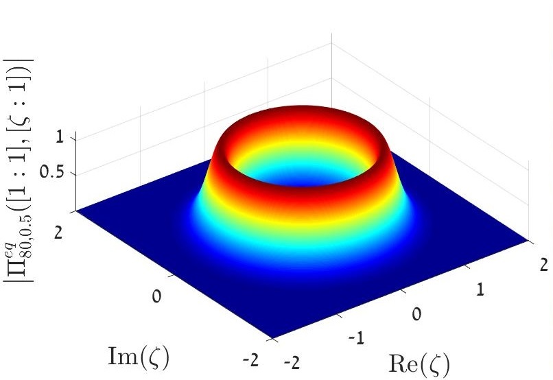
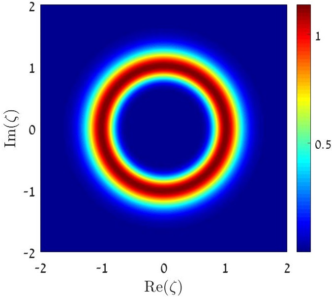
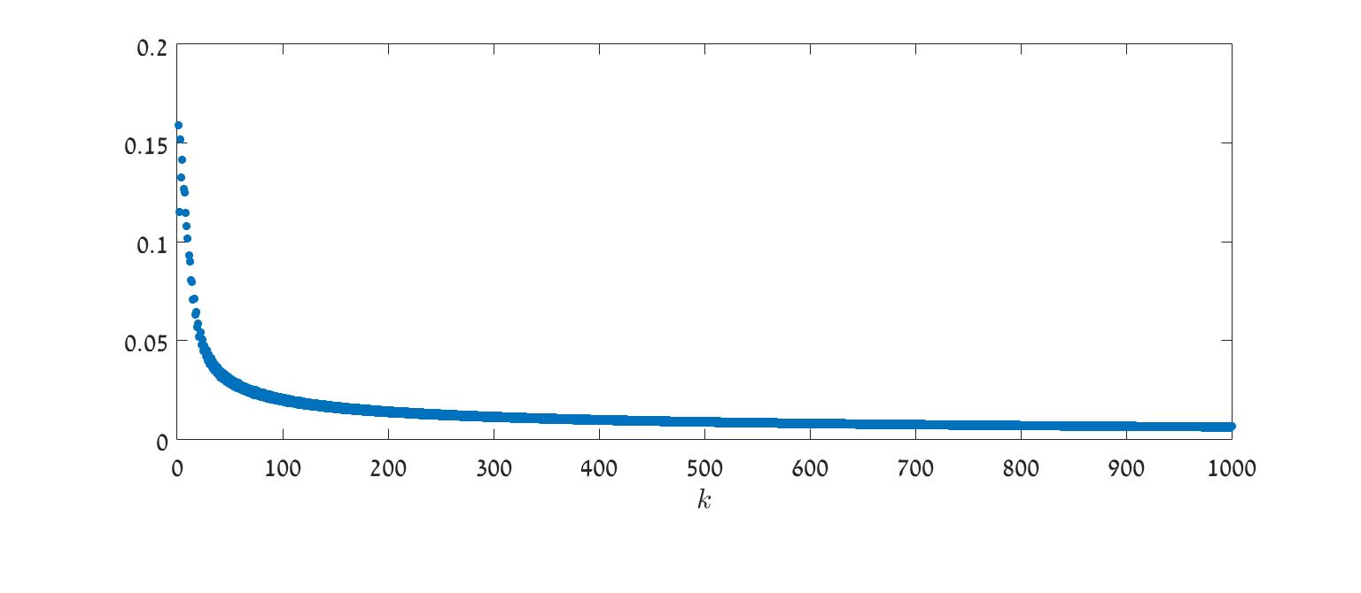
The following image illustrates the behaviour of $\mathcal{K}_{k,E}([z],[w])$ (as expected, the image appears to be in accordance with the estimate provided by Theorem 1.6).
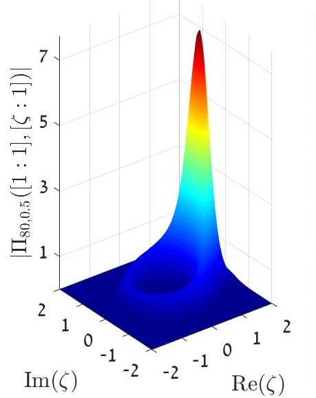
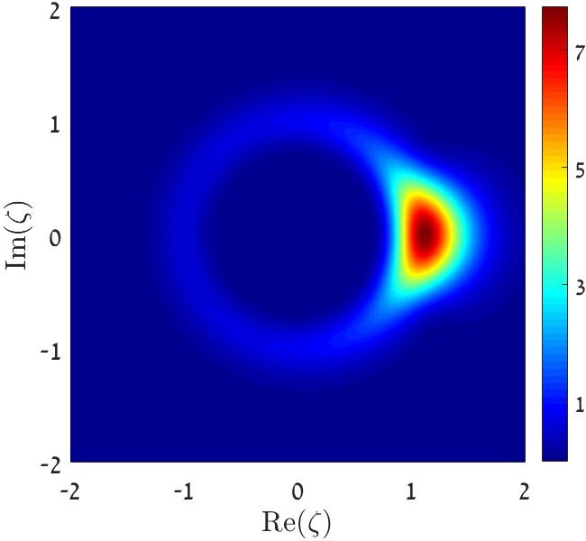
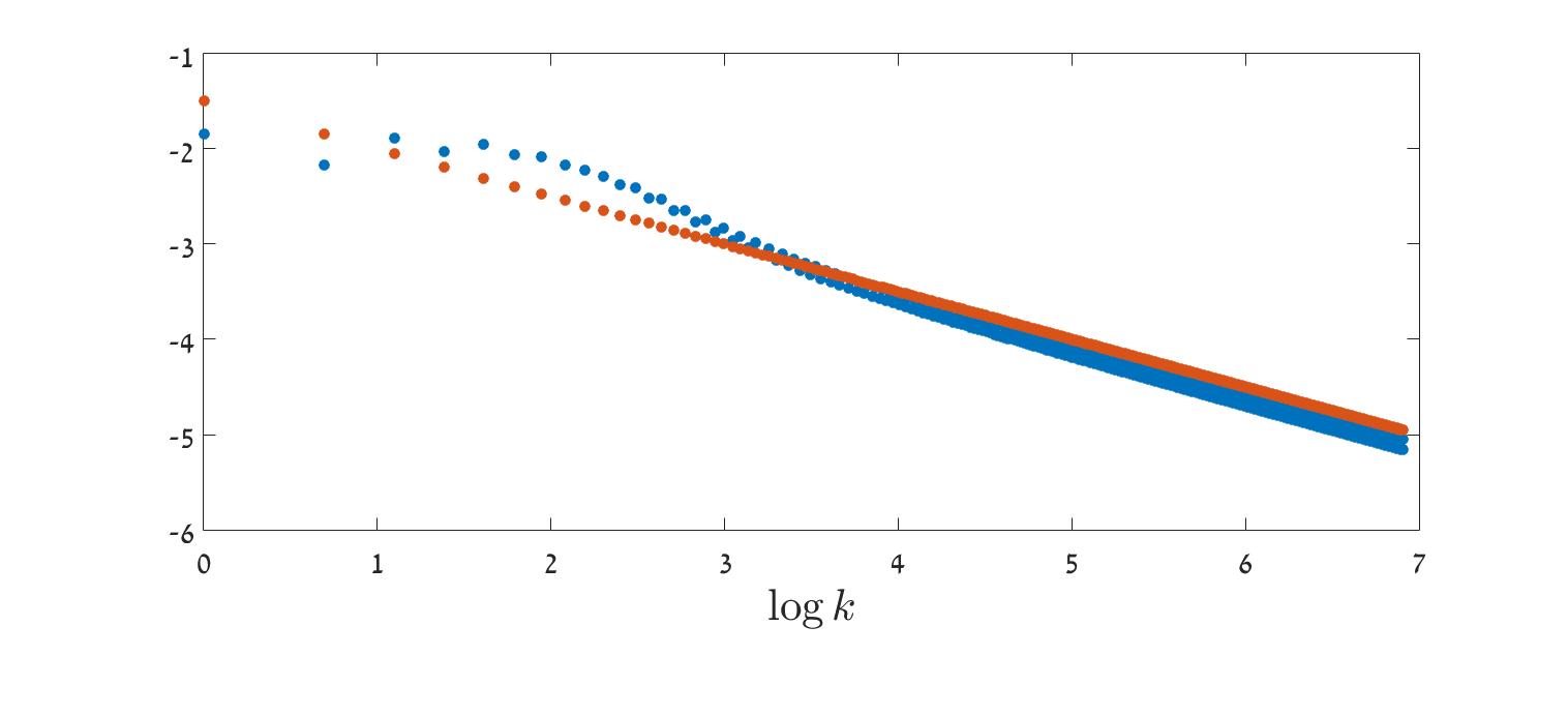
Refer to caption
Refer to caption
Figure 2: A plot of $\left|\mathcal{K}_{80,0.5}([1:1],[\zeta:1])\right|$. The circle $\{|\zeta|=1\}=\{H=0.5\}$ is the orbit of $[1:1]$, and $\zeta=1$ corresponds to the point $([1:1],[1:1])$ on the diagonal $\Delta_{\mathbb{C}P^{1}}\subset\mathbb{C}P^{1}\times\mathbb{C}P^{1}$.

Consider $[z]\in H^{-1}(E)$, and denote

$$\text{Er}_{k}(t_{0},E,[z])=\left|\mathcal{K}_{k,E}([z],[U_{t_{0}}z])-\mathcal{K}_{k,E,\text{approx}}([z],[U_{t_{0}}z])\right|,$$

where

$$\mathcal{K}_{k,E,\text{approx}}([z],[U_{t_{0}}z])=\frac{k}{4\pi}\frac{e^{-i\lceil kE\rceil t_{0}}}{\sqrt{2E(1-E)}\sqrt{\pi k}}\left(1-i\cot\left(\frac{t_{0}}{2}\right)\right)$$

is the leading term in the estimate of Theorem 1.6. The next images illustrate the behaviour of the error as $k$ grows.

Refer to caption
Refer to caption
Figure 3: A plot of $\text{Er}_{k}\left(\frac{\pi}{2},\frac{1}{2},[1:1]\right)$ as a function of $k$ (top), and (bottom) a plot of $\log\text{Er}_{k}\left(\frac{\pi}{2},\frac{1}{2},[1:1]\right)$ (in blue) and $-1.5-0.5\log(k)$ (in red) as functions of $\log(k)$. The slope of $-0.5$ is in accordance with the fact that the sub-leading term in the estimate provided by Theorem 1.6 is (in this case) of order $k^{-0.5}$.

3 The microsupport of partial Bergman kernels

3.1 Definition and basic properties

The notion of microsupport of an admissible sequence of holomorphic sections is specified in [4], as follows. Let (sk)kโˆˆโ„•subscriptsubscript๐‘ ๐‘˜๐‘˜โ„•(s_{k})_{k\in\mathbb{N}} denote a sequence such that skโˆˆโ„‹ksubscript๐‘ ๐‘˜subscriptโ„‹๐‘˜s_{k}\in\mathcal{H}_{k}. We say that (sk)kโˆˆโ„•subscriptsubscript๐‘ ๐‘˜๐‘˜โ„•(s_{k})_{k\in\mathbb{N}} is admissible if there exists $N>0$ such that โ€–skโ€–=๐’ชโ€‹(kN)normsubscript๐‘ ๐‘˜๐’ชsuperscript๐‘˜๐‘\|s_{k}\|=\mathcal{O}(k^{N}). An admissible sequence (sk)kโˆˆโ„•subscriptsubscript๐‘ ๐‘˜๐‘˜โ„•(s_{k})_{k\in\mathbb{N}} is called negligible at $z_{0}\in M$ if there exists a neighborhood $V$ of $z_{0}$ such that supzโˆˆV|skโ€‹(z)|z=๐’ชโ€‹(kโˆ’โˆž)subscriptsupremum๐‘ง๐‘‰subscriptsubscript๐‘ ๐‘˜๐‘ง๐‘ง๐’ชsuperscript๐‘˜\sup_{z\in V}|s_{k}(z)|_{z}=\mathcal{O}(k^{-\infty}), where $|\cdot|_{z}$ is the norm on $L^{\otimes k}_{z}$ induced by the Hermitian product.

Definition 3.1.

The microsupport of an admissible sequence (sk)kโˆˆโ„•subscriptsubscript๐‘ ๐‘˜๐‘˜โ„•(s_{k})_{k\in\mathbb{N}} is the set MSโก(sk)โŠ‚MMSsubscript๐‘ ๐‘˜๐‘€\operatorname{MS}(s_{k})\subset M specified by

MSโก(sk)=Mโˆ–{zโˆˆM|(sk)kโˆˆโ„•โ€‹ย is negligible atย โ€‹z}.MSsubscript๐‘ ๐‘˜๐‘€conditional-set๐‘ง๐‘€subscriptsubscript๐‘ ๐‘˜๐‘˜โ„•ย is negligible atย ๐‘ง\operatorname{MS}(s_{k})=M\setminus\{z\in M\ |\ (s_{k})_{k\in\mathbb{N}}\text{ is negligible at }z\}.

The notion of microsupport is also applicable to sequences $(T_{k})_{k\in\mathbb{N}}$ with $T_{k}\in\operatorname{End}(\mathcal{H}_{k})$. To this end, equip $M\times M$ with the symplectic form $\pi_{1}^{*}\omega-\pi_{2}^{*}\omega$, where $\pi_{1},\pi_{2}$ are the natural projections on the left and right factors. Then $\operatorname{MS}(T_{k})\subset M\times M$ is defined to be the microsupport of the sequence of Schwartz kernels of $T_{k}$, which are holomorphic sections of LโŠ—kโŠ (Lโˆ—)โŠ—kโ†’Mร—Mโ†’โŠ superscript๐ฟtensor-productabsent๐‘˜superscriptsuperscript๐ฟtensor-productabsent๐‘˜๐‘€๐‘€L^{\otimes k}\boxtimes(L^{*})^{\otimes k}\to M\times M.

Example 3.2.

([4]) Assume that Tk=ฮ kโ€‹โ„ณGkโ€‹ฮ ksubscript๐‘‡๐‘˜subscriptฮ ๐‘˜subscriptโ„ณsubscript๐บ๐‘˜subscriptฮ ๐‘˜T_{k}=\Pi_{k}\mathcal{M}_{G_{k}}\Pi_{k}, where $G_{k}\in C^{\infty}(M)$ admits the expansion $G_{k}=\sum_{l=0}^{\infty}g_{l}k^{-l}$ in the $C^{\infty}$ topology. Then $\operatorname{MS}(T_{k})\subset\Delta_{M}$, where $\Delta_{M}\subset M\times M$ is the diagonal. Viewed as a subset of $M$,

$$\operatorname{MS}(T_{k})=\overline{\cup_{l\geq 0}\operatorname{supp}(g_{l})}.$$ (4)

3.2 Proof of Theorem 1.2

The operator $\hat{F}_{k}$ admits the representation ([25], [16], Proposition 8.1.3)

F^k=ฮ kโ€‹โ„ณFโˆ’12โ€‹kโ€‹ฮ”โ€‹Fโ€‹ฮ k,subscript^๐น๐‘˜subscriptฮ ๐‘˜subscriptโ„ณ๐น12๐‘˜ฮ”๐นsubscriptฮ ๐‘˜\hat{F}_{k}=\Pi_{k}\mathcal{M}_{F-\frac{1}{2k}\Delta F}\Pi_{k}, (5)

where $\Delta$ is the Laplacian defined by the Kรคhler metric of $M$.

Lemma 3.3.

Let $\varepsilon>0$. Let $\psi_{\varepsilon}:\mathbb{R}\to[0,1]$ be a smooth function such that $\psi_{\varepsilon}(t)=0$ for all $t\leq E-\varepsilon$, $\psi_{\varepsilon}(t)=1$ for all $t\geq E$. Write $\hat{\Psi}_{k,\varepsilon}=\psi_{\varepsilon}\big{(}\hat{F_{k}}\big{)}$. Then $\operatorname{MS}(\hat{\Psi}_{k,\varepsilon})\subset\{F\geq E-\varepsilon\}$.

Proof.

There exists ([4], Proposition 12) $\Psi_{k,\varepsilon}\in C^{\infty}(M)$, admitting an expansion

$$\Psi_{k,\varepsilon}=\sum_{l=0}^{\infty}k^{-l}\psi_{l,\varepsilon}$$

in the $C^{\infty}$ topology, such that ฯˆฮตโ€‹(F^k)=ฮ kโ€‹โ„ณฮจk,ฮตโ€‹ฮ k+๐’ชโ€‹(kโˆ’โˆž)subscript๐œ“๐œ€subscript^๐น๐‘˜subscriptฮ ๐‘˜subscriptโ„ณsubscriptฮจ๐‘˜๐œ€subscriptฮ ๐‘˜๐’ชsuperscript๐‘˜\psi_{\varepsilon}(\hat{F}_{k})=\Pi_{k}\mathcal{M}_{\Psi_{k,\varepsilon}}\Pi_{k}+\mathcal{O}(k^{-\infty}). If $F(z)<E-\varepsilon$, then $\psi_{\varepsilon}$ vanishes in a neighborhood of $F(z)$, hence (using [4], p27) there exists a neighborhood $V$ of $z$ such that $\psi_{l,\varepsilon}\big{|}_{V}\equiv 0$ for all $l\geq 0$. Thus, in light of (4), $z\not\in\operatorname{MS}\big{(}\psi_{\varepsilon}(\hat{F}_{k})\big{)}$. โˆŽ

The first item of Theorem 1.2 now readily follows.

Corollary 3.4.

The microsupport of $\mathbbm{1}_{[E,\infty)}(\hat{F}_{k})$ satisfies

$$\operatorname{MS}(\mathbbm{1}_{[E,\infty)}(\hat{F}_{k}))\subset\{F\geq E\}\times\{F\geq E\}.$$

The same holds for $\mathbbm{1}_{(E,\infty)}(\hat{F}_{k})$.

Proof.

We prove for $A_{k}=\mathbbm{1}_{[E,\infty)}(\hat{F}_{k})$, but the proof for $\mathbbm{1}_{(E,\infty)}(\hat{F}_{k})$ is identical. Let $\psi_{\varepsilon}$ be as in Lemma 3.3, and write $\hat{\Psi}_{k,\varepsilon}=\psi_{\varepsilon}(\hat{F}_{k})$. Then

$$A_{k}=\hat{\Psi}_{k,\varepsilon}A_{k}=A_{k}\hat{\Psi}_{k,\varepsilon},$$

hence (using [4], p24)

$\displaystyle\operatorname{MS}(A_{k})=\operatorname{MS}(\hat{\Psi}_{k,\varepsilon}A_{k})$
$\displaystyle\subset\{(z_{1},z_{3})\ |\ \exists z_{2}\in M\ \text{such that }(z_{1},z_{2})\in\operatorname{MS}(\hat{\Psi}_{k,\varepsilon})\text{ and }(z_{2},z_{3})\in\operatorname{MS}(A_{k})\}$
$\displaystyle\subset\operatorname{MS}(\hat{\Psi}_{k,\varepsilon})\times M,$

where by a slight abuse of notation, in the second line $\operatorname{MS}(\hat{\Psi}_{k,\varepsilon})$ is viewed as a subset of $M\times M$, and in the third line it is viewed as a subset of $M$. Repeating this argument,

$$\operatorname{MS}(A_{k})=\operatorname{MS}(A_{k}\hat{\Psi}_{k,\varepsilon})\subset M\times\operatorname{MS}(\hat{\Psi}_{k,\varepsilon}),$$

therefore (noting Lemma 3.3)

$\displaystyle\operatorname{MS}(A_{k})\subset\left(\operatorname{MS}(\hat{\Psi}_{k,\varepsilon})\times M\right)\cap\left(M\times\operatorname{MS}(\hat{\Psi}_{k,\varepsilon})\right)$
$\displaystyle=\operatorname{MS}(\hat{\Psi}_{k,\varepsilon})\times\operatorname{MS}(\hat{\Psi}_{k,\varepsilon})\subset\{F\geq E-\varepsilon\}\times\{F\geq E-\varepsilon\}.$

Since $\varepsilon>0$ is arbitrary, we obtain the required. โˆŽ

The second item of Theorem 1.2 immediately follows from Corollary 3.4.

Corollary 3.5.

Replacing $F$ with $G=-F$ and $E$ with $-E$, if $G(z)<-E$ or $G(w)<-E$ then there exists a neighborhood $\mathcal{N}\subset M\times M$ of $(z,w)$ such that

$$\sup_{\mathcal{N}}\left|\mathbbm{1}_{(-E,\infty)}(\hat{G}_{k})\right|=\mathcal{O}(k^{-\infty}),$$

where

๐Ÿ™(โˆ’E,โˆž)โ€‹(G^k)=ฮ kโˆ’๐Ÿ™(โˆ’โˆž,โˆ’E]โ€‹(G^k)=ฮ kโˆ’๐Ÿ™[E,โˆž)โ€‹(F^k),subscript1๐ธsubscript^๐บ๐‘˜subscriptฮ ๐‘˜subscript1๐ธsubscript^๐บ๐‘˜subscriptฮ ๐‘˜subscript1๐ธsubscript^๐น๐‘˜\displaystyle\mathbbm{1}_{(-E,\infty)}(\hat{G}_{k})=\Pi_{k}-\mathbbm{1}_{(-\infty,-E]}(\hat{G}_{k})=\Pi_{k}-\mathbbm{1}_{[E,\infty)}(\hat{F}_{k}),

that is, sup๐’ฉ|ฮ kโˆ’๐Ÿ™[E,โˆž)โ€‹(F^k)|=๐’ชโ€‹(kโˆ’โˆž)subscriptsupremum๐’ฉsubscriptฮ ๐‘˜subscript1๐ธsubscript^๐น๐‘˜๐’ชsuperscript๐‘˜\sup_{\mathcal{N}}\left|\Pi_{k}-\mathbbm{1}_{[E,\infty)}(\hat{F}_{k})\right|=\mathcal{O}(k^{-\infty}).

Finally,

Lemma 3.6.

Corollary 3.4 implies Corollary 1.5.

Proof.

We keep the notations used in the formulation of Corollary 1.5, and also write

ฮ k,1=๐Ÿ™[E1,โˆž)โ€‹(F^k),ฮ k,2=๐Ÿ™[E2,โˆž)โ€‹(G^k).formulae-sequencesubscriptฮ ๐‘˜1subscript1subscript๐ธ1subscript^๐น๐‘˜subscriptฮ ๐‘˜2subscript1subscript๐ธ2subscript^๐บ๐‘˜\Pi_{k,1}=\mathbbm{1}_{[E_{1},\infty)}(\hat{F}_{k}),\ \Pi_{k,2}=\mathbbm{1}_{[E_{2},\infty)}(\hat{G}_{k}).

Then using Corollary 3.4,

MSโก(ฮ k,1โ€‹ฮ k,2)MSsubscriptฮ ๐‘˜1subscriptฮ ๐‘˜2\displaystyle\operatorname{MS}\left(\Pi_{k,1}\Pi_{k,2}\right)
โŠ‚{(z1,z3)|โˆƒz2โˆˆMโ€‹ย such thatย โ€‹(z1,z2)โˆˆMSโก(ฮ k,1)โ€‹ย andย โ€‹(z2,z3)โˆˆMSโก(ฮ k,2)}absentconditional-setsubscript๐‘ง1subscript๐‘ง3subscript๐‘ง2๐‘€ย such thatย subscript๐‘ง1subscript๐‘ง2MSsubscriptฮ ๐‘˜1ย andย subscript๐‘ง2subscript๐‘ง3MSsubscriptฮ ๐‘˜2\displaystyle\subset\{(z_{1},z_{3})\ |\ \exists z_{2}\in M\text{ such that }(z_{1},z_{2})\in\operatorname{MS}(\Pi_{k,1})\text{ and }(z_{2},z_{3})\in\operatorname{MS}\left(\Pi_{k,2}\right)\}
$\displaystyle\subset\{(z_{1},z_{3})\ |\ \exists z_{2}\in M\text{ such that }z_{2}\in\{F\geq E_{1}\}\cap\{G\geq E_{2}\}\}=\emptyset.$

Thus ฮ k,1โ€‹ฮ k,2subscriptฮ ๐‘˜1subscriptฮ ๐‘˜2\Pi_{k,1}\Pi_{k,2} is a negligible sequence, which implies ([4], Remark 5) that โ€–ฮ k,1โ€‹ฮ k,2โ€–op=๐’ชโ€‹(kโˆ’โˆž)subscriptnormsubscriptฮ ๐‘˜1subscriptฮ ๐‘˜2op๐’ชsuperscript๐‘˜\|\Pi_{k,1}\Pi_{k,2}\|_{\operatorname{op}}=\mathcal{O}(k^{-\infty}).โˆŽ

The proof of the first part of the first item of Theorem 1.7 is essentially identical to that of Theorem 1.2. Namely,

Lemma 3.7.

Let $\lambda_{k}$ be a sequence of eigenvalues of $\hat{F}_{k}$ with $|\lambda_{k}-E|=\mathcal{O}(k^{-1})$, where $E\in F(M)$. Let ฮ k,ฮปk,Fsubscriptฮ ๐‘˜subscript๐œ†๐‘˜๐น\Pi_{k,\lambda_{k},F} be the orthogonal projection onto the eigenspace associated with $\lambda_{k}$. Then MSโก(ฮ k,ฮปk,F)โŠ‚{F=E}ร—{F=E}MSsubscriptฮ ๐‘˜subscript๐œ†๐‘˜๐น๐น๐ธ๐น๐ธ\operatorname{MS}(\Pi_{k,\lambda_{k},F})\subset\{F=E\}\times\{F=E\}.

Proof.

Given $\varepsilon>0$ we consider a smooth function $\psi_{\varepsilon}:\mathbb{R}\to[0,1]$ such that $\psi_{\varepsilon}(t)=1$ whenever $|t-E|<\frac{\varepsilon}{2}$ and $\psi_{\varepsilon}(t)=0$ whenever $|t-E|\geq\varepsilon$. Write $\hat{\Psi}_{k,\varepsilon}=\psi_{\varepsilon}(\hat{F}_{k})$, and note that exactly as in Lemma 3.3,

$$\operatorname{MS}(\hat{\Psi}_{k,\varepsilon})\subset\{|F-E|\leq\varepsilon\}\times\{|F-E|\leq\varepsilon\}.$$

For every sufficiently large $k$, it holds that ฮจ^k,ฮตโ€‹ฮ k,ฮปk,F=ฮ k,ฮปk,Fโ€‹ฮจ^k,ฮต=ฮ k,ฮปk,Fsubscript^ฮจ๐‘˜๐œ€subscriptฮ ๐‘˜subscript๐œ†๐‘˜๐นsubscriptฮ ๐‘˜subscript๐œ†๐‘˜๐นsubscript^ฮจ๐‘˜๐œ€subscriptฮ ๐‘˜subscript๐œ†๐‘˜๐น\hat{\Psi}_{k,\varepsilon}\Pi_{k,\lambda_{k},F}=\Pi_{k,\lambda_{k},F}\hat{\Psi}_{k,\varepsilon}=\Pi_{k,\lambda_{k},F}. Thus, exactly as in Corollary 3.4, we obtain that

MSโก(ฮ k,ฮปk,F)โŠ‚MSโก(ฮจ^k,ฮต)ร—MSโก(ฯˆฮตโ€‹(F^k))โŠ‚{|Fโˆ’E|โ‰คฮต}ร—{|Fโˆ’E|โ‰คฮต}.MSsubscriptฮ ๐‘˜subscript๐œ†๐‘˜๐นMSsubscript^ฮจ๐‘˜๐œ€MSsubscript๐œ“๐œ€subscript^๐น๐‘˜๐น๐ธ๐œ€๐น๐ธ๐œ€\operatorname{MS}(\Pi_{k,\lambda_{k},F})\subset\operatorname{MS}(\hat{\Psi}_{k,\varepsilon})\times\operatorname{MS}(\psi_{\varepsilon}(\hat{F}_{k}))\subset\{|F-E|\leq\varepsilon\}\times\{|F-E|\leq\varepsilon\}.

Since $\varepsilon$ is arbitrary, MSโก(ฮ k,ฮปk)โŠ‚{F=E}ร—{F=E}MSsubscriptฮ ๐‘˜subscript๐œ†๐‘˜๐น๐ธ๐น๐ธ\operatorname{MS}(\Pi_{k,\lambda_{k}})\subset\{F=E\}\times\{F=E\}. โˆŽ

4 Fourier theory and partial Bergman kernels

4.1 The Cauchy-Szegรถ projection on the circle

Let $\mathbb{R}/2\pi\mathbb{Z}=S^{1}\subset\mathbb{C}$ denote the unit circle. Let $\hat{g}(p)=\langle g,e_{p}\rangle_{L^{2}(S^{1})}$ denote the $p$-th Fourier coefficient of $g\in L^{1}(S^{1})$, where $p\in\mathbb{Z}$ and $e_{p}(t)=e^{ipt}$. The Cauchy-Szegรถ projection ฮ S1:L2โ€‹(S1)โ†’H2โ€‹(S1):subscriptฮ superscript๐‘†1โ†’superscript๐ฟ2superscript๐‘†1superscript๐ป2superscript๐‘†1\Pi_{S^{1}}:L^{2}(S^{1})\to H^{2}(S^{1}) is the orthogonal projection on the Hardy space

$$H^{2}(S^{1})=\left\{g\in L^{2}(S^{1})\ |\ \hat{g}(p)=0\ \forall p<0\right\},$$

and it admits the formula

ฮ S1โ€‹(g)โ€‹(t)=limrโ†’1โˆ’12โ€‹ฯ€โ€‹โˆซโˆ’ฯ€ฯ€gโ€‹(tโˆ’s)1โˆ’rโ€‹eiโ€‹sโ€‹๐‘‘s.subscriptฮ superscript๐‘†1๐‘”๐‘กsubscriptโ†’๐‘Ÿsuperscript112๐œ‹superscriptsubscript๐œ‹๐œ‹๐‘”๐‘ก๐‘ 1๐‘Ÿsuperscript๐‘’๐‘–๐‘ differential-d๐‘ \Pi_{S^{1}}(g)(t)=\lim_{r\to 1^{-}}\frac{1}{2\pi}\int_{-\pi}^{\pi}\frac{g(t-s)}{1-re^{is}}ds.

The periodic Hilbert transform $\mathcal{H}_{S^{1}}:L^{2}(S^{1})\to L^{2}(S^{1})$ is specified by $\mathcal{H}_{S^{1}}(e_{p})=-i\operatorname{sgn}(p)e_{p}$, or equivalently

โ„‹S1โ€‹(g)โ€‹(t)=limฮตโ†’0+12โ€‹ฯ€โ€‹โˆซฮตโ‰ค|tโˆ’s|โ‰คฯ€gโ€‹(s)โ€‹cotโก(tโˆ’s2)โ€‹๐‘‘s.subscriptโ„‹superscript๐‘†1๐‘”๐‘กsubscriptโ†’๐œ€superscript012๐œ‹subscript๐œ€๐‘ก๐‘ ๐œ‹๐‘”๐‘ ๐‘ก๐‘ 2differential-d๐‘ \mathcal{H}_{S^{1}}(g)(t)=\lim_{\varepsilon\to 0^{+}}\frac{1}{2\pi}\int_{\varepsilon\leq|t-s|\leq\pi}g(s)\cot\left(\frac{t-s}{2}\right)ds.
Corollary 4.1.

The Cauchy-Szegรถ projection acts by $e_{p}(t)\mapsto\mathbbm{1}_{[0,\infty)}(p)e_{p}(t)$, hence it can be expressed in terms of the periodic Hilbert transform, as follows:

ฮ S1โ€‹(g)=12โ€‹(iโ€‹โ„‹S1โ€‹(g)+g+g^โ€‹(0)).subscriptฮ superscript๐‘†1๐‘”12๐‘–subscriptโ„‹superscript๐‘†1๐‘”๐‘”^๐‘”0\Pi_{S^{1}}(g)=\frac{1}{2}\left(i\mathcal{H}_{S^{1}}(g)+g+\hat{g}(0)\right).

4.2 Spectral projections and unitary representations of $S^{1}$

Let $\mathcal{H}$ denote a finite dimensional complex Hilbert space, and write $\dim\mathcal{H}=d$. Let $A\in\operatorname{End}(\mathcal{H})$ be a Hermitian operator. Denote

$$U_{A}(t)=e^{itA},$$

and assume that $t\mapsto U_{A}(t)$ is $2\pi$-periodic.

Let $v_{1},...,v_{d}$ be an orthonormal eigenbasis of $A$ such that $Av_{m}=p_{m}v_{m}$, with $p_{1}\leq p_{2}\leq...\leq p_{d}$. Then $p_{m}\in\mathbb{Z}$, and we can write

$$A=\sum_{m=1}^{d}p_{m}v_{m}\otimes v_{m}^{*},\ U_{A}(t)=\sum_{m=1}^{d}e^{itp_{m}}v_{m}\otimes v_{m}^{*},$$

where $v_{m}^{*}$ is the dual vector of $v_{m}$.

Corollary 4.2.

The spectral projection ฮ A=๐Ÿ™[0,โˆž)โ€‹(A)subscriptฮ ๐ดsubscript10๐ด\Pi_{A}=\mathbbm{1}_{[0,\infty)}(A) can be written in the following form:

ฮ A=(ฮ S1โ€‹(UA))โ€‹(0)=limrโ†’1โˆ’12โ€‹ฯ€โ€‹โˆซโˆ’ฯ€ฯ€UAโ€‹(s)1โˆ’rโ€‹eiโ€‹sโ€‹๐‘‘s.subscriptฮ ๐ดsubscriptฮ superscript๐‘†1subscript๐‘ˆ๐ด0subscriptโ†’๐‘Ÿsuperscript112๐œ‹superscriptsubscript๐œ‹๐œ‹subscript๐‘ˆ๐ด๐‘ 1๐‘Ÿsuperscript๐‘’๐‘–๐‘ differential-d๐‘ \Pi_{A}=\left(\Pi_{S^{1}}(U_{A})\right)(0)=\lim_{r\to 1^{-}}\frac{1}{2\pi}\int_{-\pi}^{\pi}\frac{U_{A}(s)}{1-re^{is}}ds.

In terms of the Hilbert transform,

ฮ A=12โ€‹(iโ€‹โ„‹S1โ€‹(UA)โ€‹(0)+Idโ„‹+U^Aโ€‹(0)),subscriptฮ ๐ด12๐‘–subscriptโ„‹superscript๐‘†1subscript๐‘ˆ๐ด0subscriptIdโ„‹subscript^๐‘ˆ๐ด0\Pi_{A}=\frac{1}{2}\left(i\mathcal{H}_{S^{1}}(U_{A})(0)+\operatorname{Id}_{\mathcal{H}}+\widehat{U}_{A}(0)\right), (6)

where

$$\widehat{U}_{A}(0)=\frac{1}{2\pi}\int_{-\pi}^{\pi}U_{A}(t)dt$$

and

$$\mathcal{H}_{S^{1}}(U_{A})(0)=\frac{1}{2\pi}\int_{0}^{\pi}\left(U_{A}(-t)-U_{A}(t)\right)\cot\left(\frac{t}{2}\right)dt.$$

More generally, given $p,p_{0}\in\mathbb{Z}$ and $g\in L^{2}(S^{1})$, recall that

$$\widehat{e_{-p_{0}}g}(p)=\langle e_{-p_{0}}g,e_{p}\rangle_{L^{2}(S^{1})}=\langle g,e_{p+p_{0}}\rangle_{L^{2}(S^{1})}=\hat{g}(p+p_{0}).$$

This relation allows us to extend formula (6) to ฮ A,E=๐Ÿ™[E,โˆž)โ€‹(A)subscriptฮ ๐ด๐ธsubscript1๐ธ๐ด\Pi_{A,E}=\mathbbm{1}_{[E,\infty)}(A), $E\in\mathbb{R}$.

Corollary 4.3.

Let $E\in\mathbb{R}$. Denote $U_{A,E}=e_{-\lceil E\rceil}U_{A}$. Then

ฮ A,E=(ฮ S1โ€‹(UA,E))โ€‹(0)=12โ€‹(iโ€‹โ„‹S1โ€‹(UA,E)โ€‹(0)+Idโ„‹+U^A,Eโ€‹(0)),subscriptฮ ๐ด๐ธsubscriptฮ superscript๐‘†1subscript๐‘ˆ๐ด๐ธ012๐‘–subscriptโ„‹superscript๐‘†1subscript๐‘ˆ๐ด๐ธ0subscriptIdโ„‹subscript^๐‘ˆ๐ด๐ธ0\Pi_{A,E}=\left(\Pi_{S^{1}}(U_{A,E})\right)(0)=\frac{1}{2}\left(i\mathcal{H}_{S^{1}}(U_{A,E})(0)+\operatorname{Id}_{\mathcal{H}}+\widehat{U}_{A,E}(0)\right), (7)

where

$$\widehat{U}_{A,E}(0)=\frac{1}{2\pi}\int_{-\pi}^{\pi}U_{A,E}(t)dt=\frac{1}{2\pi}\int_{-\pi}^{\pi}U_{A}(t)e^{-i\lceil E\rceil t}dt$$

and

$$\mathcal{H}_{S^{1}}(U_{A,E})(0)=\frac{1}{2\pi}\int_{0}^{\pi}\left(U_{A}(-t)e^{i\lceil E\rceil t}-U_{A}(t)e^{-i\lceil E\rceil t}\right)\cot\left(\frac{t}{2}\right)dt.$$

4.3 Proof of Theorems 1.6, 1.7

The proof of Theorem 1.6 relies on formula (7), which is also applicable to the Schwartz kernels of the operators involved. Thus, we obtain a representation of ฮ k,Eโ€‹(z,w)subscriptฮ ๐‘˜๐ธ๐‘ง๐‘ค\Pi_{k,E}(z,w) in terms of the Bergman kernel and the Schwartz kernel of the quantum propagator defined by $\hat{H}_{k}$. The well-known asymptotic properties of the Bergman kernel, with the help of the stationary phase lemma, produce the desired estimate. Notably, we can assume without loss of generality that the circle action is effective (Lemma 4.4), and then the third term in (7) is the equivariant Bergman projection associated with the eigenvalue $\frac{\lceil kE\rceil}{k}$ of $\hat{H}_{k}$. Accordingly, the proof of Theorem 1.6 relies on the second item of Theorem 1.7. The latter is established by similar arguments, namely, the stationary phase lemma is used together with the integral representation of equivariant Bergman kernels as โ€Fourier coefficientsโ€ of the full Bergman kernel.

Recall that there exists $N\geq 1$ and an open dense subset $M_{N}\subset M$ such that the stabilizer group of every $z\in M_{N}$ is the subgroup $S^{1}_{N}\subset S^{1}$ of order $N$. We assume throughout that $N=1$ (i.e., that the circle action is effective); this is justified by the following lemma.

Lemma 4.4.

It suffices to prove Theorems 1.6, 1.7 in the case $N=1$.

Proof.

Assume that $N>1$. If $t\in S^{1}_{N}$, then $\varphi_{t}|_{M_{N}}=\operatorname{Id}$, hence by continuity $\varphi_{t}=\operatorname{Id}$. It follows that $t\mapsto\varphi_{N,t}=\varphi_{\frac{t}{N}}$, $t\in\mathbb{R}/2\pi\mathbb{Z}$, is an effective holomorphic circle action, generated by the Hamiltonian $H_{N}=\frac{1}{N}H$. Writing $\hat{H}_{N,k}=\frac{1}{N}\hat{H}_{k}$,

ฮ k,E=๐Ÿ™[E,โˆž)โ€‹(H^k)=๐Ÿ™[EN,โˆž)โ€‹(H^N,k).subscriptฮ ๐‘˜๐ธsubscript1๐ธsubscript^๐ป๐‘˜subscript1๐ธ๐‘subscript^๐ป๐‘๐‘˜\Pi_{k,E}=\mathbbm{1}_{[E,\infty)}(\hat{H}_{k})=\mathbbm{1}_{[\frac{E}{N},\infty)}\left(\hat{H}_{N,k}\right).

Thus, the case $N>1$ is reduced to the case $N=1$. Similarly,

ฮ k,ฮปkeq=๐Ÿ™{ฮปk}โ€‹(H^k)=๐Ÿ™{ฮปkN}โ€‹(H^N,k).subscriptsuperscriptฮ eq๐‘˜subscript๐œ†๐‘˜subscript1subscript๐œ†๐‘˜subscript^๐ป๐‘˜subscript1subscript๐œ†๐‘˜๐‘subscript^๐ป๐‘๐‘˜\Pi^{\operatorname{eq}}_{k,\lambda_{k}}=\mathbbm{1}_{\{\lambda_{k}\}}(\hat{H}_{k})=\mathbbm{1}_{\{\frac{\lambda_{k}}{N}\}}(\hat{H}_{N,k}).

โˆŽ

Recall that $E\in H(M)$ is a regular value of $H$, and assume that $z\in H^{-1}(E)$. Denote $V_{k}(t)=e^{ikt\hat{H}_{k}}$, and consider the map

$$V_{k}(z,w):S^{1}\to L_{z}^{\otimes k}\otimes(L_{w}^{*})^{\otimes k}$$

specified by $t\mapsto V_{k}(t)(z,w)$, where the latter is the Schwartz kernel of $V_{k}(t)$. Denote $E_{k}=\frac{\lceil kE\rceil}{k}$ and $V_{k,E_{k}}(t)(z,w)=e^{-ikE_{k}t}V_{k}(t)(z,w)$. According to (7),

ฮ k,Eโ€‹(z,w)=12โ€‹(iโ€‹โ„‹S1โ€‹(Vk,Ekโ€‹(z,w))โ€‹(0)+ฮ kโ€‹(z,w)+Vk,Ekโ€‹(z,w)^โ€‹(0)),subscriptฮ ๐‘˜๐ธ๐‘ง๐‘ค12๐‘–subscriptโ„‹superscript๐‘†1subscript๐‘‰๐‘˜subscript๐ธ๐‘˜๐‘ง๐‘ค0subscriptฮ ๐‘˜๐‘ง๐‘ค^subscript๐‘‰๐‘˜subscript๐ธ๐‘˜๐‘ง๐‘ค0\Pi_{k,E}(z,w)=\frac{1}{2}\left(i\mathcal{H}_{S^{1}}\left(V_{k,E_{k}}(z,w)\right)(0)+\Pi_{k}(z,w)+\widehat{V_{k,E_{k}}(z,w)}(0)\right), (8)

where

Vk,Ekโ€‹(z,w)^โ€‹(0)=12โ€‹ฯ€โ€‹โˆซ02โ€‹ฯ€Vk,Ekโ€‹(t)โ€‹(z,w)โ€‹๐‘‘t=ฮ k,Ekeqโ€‹(z,w)^subscript๐‘‰๐‘˜subscript๐ธ๐‘˜๐‘ง๐‘ค012๐œ‹superscriptsubscript02๐œ‹subscript๐‘‰๐‘˜subscript๐ธ๐‘˜๐‘ก๐‘ง๐‘คdifferential-d๐‘กsubscriptsuperscriptฮ eq๐‘˜subscript๐ธ๐‘˜๐‘ง๐‘ค\widehat{V_{k,E_{k}}(z,w)}(0)=\frac{1}{2\pi}\int_{0}^{2\pi}V_{k,E_{k}}(t)(z,w)dt=\Pi^{\operatorname{eq}}_{k,E_{k}}(z,w)

is the equivariant Bergman kernel associated with the eigenvalue $E_{k}$ of $\hat{H}_{k}$. The Schwartz kernel of $V_{k,E_{k}}(t)$ admits the following useful formula.

Lemma 4.5.

The Schwartz kernel of $V_{k,E_{k}}(t)$ is specified by

Vk,Ekโ€‹(t)โ€‹(z,w)=ck,Ekโ€‹(z,t)โ€‹๐’ฏk,tโ€‹(ฮ kโ€‹(ฯ†tโ€‹(z),w)),subscript๐‘‰๐‘˜subscript๐ธ๐‘˜๐‘ก๐‘ง๐‘คsubscript๐‘๐‘˜subscript๐ธ๐‘˜๐‘ง๐‘กsubscript๐’ฏ๐‘˜๐‘กsubscriptฮ ๐‘˜subscript๐œ‘๐‘ก๐‘ง๐‘คV_{k,E_{k}}(t)(z,w)=c_{k,E_{k}}(z,t)\mathcal{T}_{k,t}\left(\Pi_{k}(\varphi_{t}(z),w)\right),

where $\mathcal{T}_{k,t}:L^{\otimes k}_{\varphi_{t}(z)}\otimes(L^{*})^{\otimes k}_{w}\to L^{\otimes k}_{z}\otimes(L^{*})^{\otimes k}_{w}$ is the parallel transport along the curve $t^{\prime}\mapsto\left(\varphi_{t-t^{\prime}}(z),w\right)$, $t^{\prime}\in[0,t]$, and $c_{k,E_{k}}(z,t)=e^{ik(H(z)-E_{k})t}=e^{ik(E-E_{k})t}$.

Proof.

As shown in [16], Proposition 8.2.1, the action of $V_{k}(t)$ is specified by

Vkโ€‹(t)โ€‹sโ€‹(z)=eiโ€‹kโ€‹tโ€‹Hโ€‹(z)โ€‹ฯ„k,tโ€‹sโ€‹(ฯ†tโ€‹(z)),sโˆˆโ„‹k,formulae-sequencesubscript๐‘‰๐‘˜๐‘ก๐‘ ๐‘งsuperscript๐‘’๐‘–๐‘˜๐‘ก๐ป๐‘งsubscript๐œ๐‘˜๐‘ก๐‘ subscript๐œ‘๐‘ก๐‘ง๐‘ subscriptโ„‹๐‘˜V_{k}(t)s(z)=e^{iktH(z)}\tau_{k,t}s(\varphi_{t}(z)),\ s\in\mathcal{H}_{k},

where $\tau_{k,t}:L^{\otimes k}_{\varphi_{t}(z)}\to L^{\otimes k}_{z}$ is the parallel transport along the curve $t^{\prime}\mapsto\varphi_{t-t^{\prime}}(z)$, $t^{\prime}\in[0,t]$. Thus, considering any orthonormal basis s1,โ€ฆ,sdksubscript๐‘ 1โ€ฆsubscript๐‘ subscript๐‘‘๐‘˜s_{1},...,s_{d_{k}} of $\mathcal{H}_{k}$, we find that the Schwartz kernel of $V_{k}(t)$ is given by

$\displaystyle V_{k}(t)(z,w)$ =โˆ‘m=1dk(Vkโ€‹(t)โ€‹sm)โ€‹(z)โŠ—smโˆ—โ€‹(w)absentsuperscriptsubscript๐‘š1subscript๐‘‘๐‘˜tensor-productsubscript๐‘‰๐‘˜๐‘กsubscript๐‘ ๐‘š๐‘งsuperscriptsubscript๐‘ ๐‘š๐‘ค\displaystyle=\sum_{m=1}^{d_{k}}\left(V_{k}(t)s_{m}\right)(z)\otimes s_{m}^{*}(w)
=eiโ€‹kโ€‹tโ€‹Hโ€‹(z)โ€‹โˆ‘m=1dk(ฯ„k,tโ€‹sm)โ€‹(ฯ†tโ€‹(z))โŠ—smโˆ—โ€‹(w)absentsuperscript๐‘’๐‘–๐‘˜๐‘ก๐ป๐‘งsuperscriptsubscript๐‘š1subscript๐‘‘๐‘˜tensor-productsubscript๐œ๐‘˜๐‘กsubscript๐‘ ๐‘šsubscript๐œ‘๐‘ก๐‘งsuperscriptsubscript๐‘ ๐‘š๐‘ค\displaystyle=e^{iktH(z)}\sum_{m=1}^{d_{k}}\left(\tau_{k,t}s_{m}\right)(\varphi_{t}(z))\otimes s_{m}^{*}(w)
=eiโ€‹kโ€‹tโ€‹Hโ€‹(z)โ€‹(ฯ„k,tโŠ—Id)โ€‹(โˆ‘m=1dksmโ€‹(ฯ†tโ€‹(z))โŠ—smโˆ—โ€‹(w))absentsuperscript๐‘’๐‘–๐‘˜๐‘ก๐ป๐‘งtensor-productsubscript๐œ๐‘˜๐‘กIdsuperscriptsubscript๐‘š1subscript๐‘‘๐‘˜tensor-productsubscript๐‘ ๐‘šsubscript๐œ‘๐‘ก๐‘งsuperscriptsubscript๐‘ ๐‘š๐‘ค\displaystyle=e^{iktH(z)}\left(\tau_{k,t}\otimes\operatorname{Id}\right)\left(\sum_{m=1}^{d_{k}}s_{m}(\varphi_{t}(z))\otimes s_{m}^{*}(w)\right)
=eiโ€‹kโ€‹tโ€‹Hโ€‹(z)โ€‹๐’ฏk,tโ€‹(ฮ kโ€‹(ฯ†tโ€‹(z),w)).absentsuperscript๐‘’๐‘–๐‘˜๐‘ก๐ป๐‘งsubscript๐’ฏ๐‘˜๐‘กsubscriptฮ ๐‘˜subscript๐œ‘๐‘ก๐‘ง๐‘ค\displaystyle=e^{iktH(z)}\mathcal{T}_{k,t}\left(\Pi_{k}(\varphi_{t}(z),w)\right).

Multiplying both sides by $e^{-ikE_{k}t}$, we obtain the required. โˆŽ

The microsupport MSโก(ฮ k)MSsubscriptฮ ๐‘˜\operatorname{MS}(\Pi_{k}) of ฮ ksubscriptฮ ๐‘˜\Pi_{k} equals the diagonal $\Delta_{M}\subset M\times M$. In particular, this implies (see [4], Proposition 8, or [19], Theorem 1) that for every $\varepsilon>0$ and $N>0$ there exists $C_{\varepsilon,N}>0$ such that for every $z,w\in M$, if $\operatorname{dist}(z,w)\geq\varepsilon$ then

|ฮ kโ€‹(z,w)|<Cฮต,Nโ€‹kโˆ’N,subscriptฮ ๐‘˜๐‘ง๐‘คsubscript๐ถ๐œ€๐‘superscript๐‘˜๐‘\lvert\Pi_{k}(z,w)\rvert<C_{\varepsilon,N}k^{-N}, (9)

and that for every vector field $Y$ on $M\times M$ there exists $C_{Y,\varepsilon,N}$ such that for every $z,w\in M$, if $\operatorname{dist}(z,w)\geq\varepsilon$ then

|(โˆ‡~k)Yโ€‹ฮ kโ€‹(z,w)|<CY,ฮต,Nโ€‹kโˆ’N.subscriptsubscript~โˆ‡๐‘˜๐‘Œsubscriptฮ ๐‘˜๐‘ง๐‘คsubscript๐ถ๐‘Œ๐œ€๐‘superscript๐‘˜๐‘\lvert(\tilde{\nabla}_{k})_{Y}\Pi_{k}(z,w)\rvert<C_{Y,\varepsilon,N}k^{-N}. (10)

Here, $\tilde{\nabla}_{k}$ is the connection on LโŠ—kโŠ (Lโˆ—)โŠ—kโŠ superscript๐ฟtensor-productabsent๐‘˜superscriptsuperscript๐ฟtensor-productabsent๐‘˜L^{\otimes k}\boxtimes(L^{*})^{\otimes k} induced by $\nabla$. The first part of Theorem 1.6 readily follows from these estimates.

Lemma 4.6.

If $z\in M$ and $w\in M\setminus\mathcal{O}_{z}$, then (z,w)โˆ‰MSโก(ฮ k,E)๐‘ง๐‘คMSsubscriptฮ ๐‘˜๐ธ(z,w)\not\in\operatorname{MS}(\Pi_{k,E}).

Proof.

Let $\mathcal{N}_{0}\subset M\times M$ denote a neighborhood of $(z,w)$ such that for every $(z^{\prime},w^{\prime})\in\mathcal{N}_{0}$ and $t\in[-\pi,\pi]$,

$$\operatorname{dist}(\varphi_{t}(z^{\prime}),w^{\prime})>\frac{\varepsilon}{2}$$

for some $\varepsilon>0$. We wish to prove that

sup๐’ฉ0|ฮ k,E|=๐’ชโ€‹(kโˆ’โˆž),subscriptsupremumsubscript๐’ฉ0subscriptฮ ๐‘˜๐ธ๐’ชsuperscript๐‘˜\sup_{\mathcal{N}_{0}}\lvert\Pi_{k,E}\rvert=\mathcal{O}(k^{-\infty}),

which would mean (by definition) that (z,w)โˆ‰MSโก(ฮ k,E)๐‘ง๐‘คMSsubscriptฮ ๐‘˜๐ธ(z,w)\not\in\operatorname{MS}(\Pi_{k,E}). Let

$$\mathcal{N}=\{(\varphi_{t}(z^{\prime}),w^{\prime})\ |\ (z^{\prime},w^{\prime})\in\mathcal{N}_{0},\ t\in[-\pi,\pi]\}.$$

Looking at the representation (8) in light of (9), we immediately note that the second term satisfies

sup๐’ฉ0|ฮ k|=๐’ชโ€‹(kโˆ’โˆž).subscriptsupremumsubscript๐’ฉ0subscriptฮ ๐‘˜๐’ชsuperscript๐‘˜\sup_{\mathcal{N}_{0}}|\Pi_{k}|=\mathcal{O}(k^{-\infty}).

Similarly, estimate (9) implies that the term Vk,Ekโ€‹(zโ€ฒ,wโ€ฒ)^โ€‹(0)=ฮ k,Ekeqโ€‹(zโ€ฒ,wโ€ฒ)^subscript๐‘‰๐‘˜subscript๐ธ๐‘˜superscript๐‘งโ€ฒsuperscript๐‘คโ€ฒ0subscriptsuperscriptฮ eq๐‘˜subscript๐ธ๐‘˜superscript๐‘งโ€ฒsuperscript๐‘คโ€ฒ\widehat{V_{k,E_{k}}(z^{\prime},w^{\prime})}(0)=\Pi^{\operatorname{eq}}_{k,E_{k}}(z^{\prime},w^{\prime}), which is the equivariant Bergman kernel associated with the eigenvalue $E_{k}$, satisfies

sup(zโ€ฒ,wโ€ฒ)โˆˆ๐’ฉ0|ฮ k,Ekeqโ€‹(zโ€ฒ,wโ€ฒ)|โ‰คsup๐’ฉ012โ€‹ฯ€โ€‹โˆซโˆ’ฯ€ฯ€|ฮ kโ€‹(ฯ†tโ€‹(zโ€ฒ),wโ€ฒ)|โ€‹๐‘‘t=๐’ชโ€‹(kโˆ’โˆž).subscriptsupremumsuperscript๐‘งโ€ฒsuperscript๐‘คโ€ฒsubscript๐’ฉ0subscriptsuperscriptฮ eq๐‘˜subscript๐ธ๐‘˜superscript๐‘งโ€ฒsuperscript๐‘คโ€ฒsubscriptsupremumsubscript๐’ฉ012๐œ‹superscriptsubscript๐œ‹๐œ‹subscriptฮ ๐‘˜subscript๐œ‘๐‘กsuperscript๐‘งโ€ฒsuperscript๐‘คโ€ฒdifferential-d๐‘ก๐’ชsuperscript๐‘˜\sup_{(z^{\prime},w^{\prime})\in\mathcal{N}_{0}}\left|\Pi^{\operatorname{eq}}_{k,E_{k}}(z^{\prime},w^{\prime})\right|\leq\sup_{\mathcal{N}_{0}}\frac{1}{2\pi}\int_{-\pi}^{\pi}\left|\Pi_{k}\left(\varphi_{t}(z^{\prime}),w^{\prime}\right)\right|dt=\mathcal{O}(k^{-\infty}). (11)

Finally, consider the first term in (8). Let $V^{\prime}_{k,E_{k}}(u)(z^{\prime},w^{\prime})=\frac{d}{dt}\big{(}V_{k}(z^{\prime},w^{\prime})\big{)}(u)$. Note that Vk,Ekโ€‹(0)โ€‹(zโ€ฒ,wโ€ฒ)=ฮ kโ€‹(zโ€ฒ,wโ€ฒ)subscript๐‘‰๐‘˜subscript๐ธ๐‘˜0superscript๐‘งโ€ฒsuperscript๐‘คโ€ฒsubscriptฮ ๐‘˜superscript๐‘งโ€ฒsuperscript๐‘คโ€ฒV_{k,E_{k}}(0)(z^{\prime},w^{\prime})=\Pi_{k}(z^{\prime},w^{\prime}). If $t\in(0,\pi)$, then by the mean-value theorem,

|Vk,Ekโ€‹(t)โ€‹(zโ€ฒ,wโ€ฒ)โˆ’ฮ kโ€‹(zโ€ฒ,wโ€ฒ)|โ‰คtโ€‹supuโˆˆ[0,t]|Vk,Ekโ€ฒโ€‹(u)โ€‹(zโ€ฒ,wโ€ฒ)|,subscript๐‘‰๐‘˜subscript๐ธ๐‘˜๐‘กsuperscript๐‘งโ€ฒsuperscript๐‘คโ€ฒsubscriptฮ ๐‘˜superscript๐‘งโ€ฒsuperscript๐‘คโ€ฒ๐‘กsubscriptsupremum๐‘ข0๐‘กsuperscriptsubscript๐‘‰๐‘˜subscript๐ธ๐‘˜โ€ฒ๐‘ขsuperscript๐‘งโ€ฒsuperscript๐‘คโ€ฒ|V_{k,E_{k}}(t)(z^{\prime},w^{\prime})-\Pi_{k}(z^{\prime},w^{\prime})|\leq t\sup_{u\in[0,t]}\left|V_{k,E_{k}}^{\prime}(u)(z^{\prime},w^{\prime})\right|,

where (in light of Lemma 4.5)

Vk,Ekโ€ฒโ€‹(u)โ€‹(zโ€ฒ,wโ€ฒ)=ck,Ekโ€‹(u)โ€‹๐’ฏk,uโ€‹(iโ€‹kโ€‹(Eโˆ’Ek)โ€‹ฮ kโ€‹(ฯ†uโ€‹(zโ€ฒ),wโ€ฒ)+(โˆ‡~k)YHโ€‹(ฮ k)โ€‹(ฯ†uโ€‹(zโ€ฒ),wโ€ฒ)),subscriptsuperscript๐‘‰โ€ฒ๐‘˜subscript๐ธ๐‘˜๐‘ขsuperscript๐‘งโ€ฒsuperscript๐‘คโ€ฒsubscript๐‘๐‘˜subscript๐ธ๐‘˜๐‘ขsubscript๐’ฏ๐‘˜๐‘ข๐‘–๐‘˜๐ธsubscript๐ธ๐‘˜subscriptฮ ๐‘˜subscript๐œ‘๐‘ขsuperscript๐‘งโ€ฒsuperscript๐‘คโ€ฒsubscriptsubscript~โˆ‡๐‘˜subscript๐‘Œ๐ปsubscriptฮ ๐‘˜subscript๐œ‘๐‘ขsuperscript๐‘งโ€ฒsuperscript๐‘คโ€ฒV^{\prime}_{k,E_{k}}(u)(z^{\prime},w^{\prime})=\\ c_{k,E_{k}}(u)\mathcal{T}_{k,u}\left(ik(E-E_{k})\Pi_{k}(\varphi_{u}(z^{\prime}),w^{\prime})+(\tilde{\nabla}_{k})_{Y_{H}}(\Pi_{k})(\varphi_{u}(z^{\prime}),w^{\prime})\right),

with $Y_{H}=(X_{H},0)$.

Applying (9) and (10), we see that

$\displaystyle\left|V^{\prime}_{k,E_{k}}(u)(z^{\prime},w^{\prime})\right|$ โ‰คkโ€‹|Eโˆ’Ek|โ€‹|ฮ kโ€‹(ฯ†uโ€‹(zโ€ฒ),wโ€ฒ)|+|(โˆ‡~k)YHโ€‹ฮ kโ€‹(ฯ†uโ€‹(zโ€ฒ),wโ€ฒ)|absent๐‘˜๐ธsubscript๐ธ๐‘˜subscriptฮ ๐‘˜subscript๐œ‘๐‘ขsuperscript๐‘งโ€ฒsuperscript๐‘คโ€ฒsubscriptsubscript~โˆ‡๐‘˜subscript๐‘Œ๐ปsubscriptฮ ๐‘˜subscript๐œ‘๐‘ขsuperscript๐‘งโ€ฒsuperscript๐‘คโ€ฒ\displaystyle\leq k|E-E_{k}||\Pi_{k}(\varphi_{u}(z^{\prime}),w^{\prime})|+|(\tilde{\nabla}_{k})_{Y_{H}}\Pi_{k}(\varphi_{u}(z^{\prime}),w^{\prime})| (12)
โ‰คsup๐’ฉ|ฮ k|+sup๐’ฉ|(โˆ‡~k)YHโ€‹ฮ k|=๐’ชโ€‹(kโˆ’โˆž).absentsubscriptsupremum๐’ฉsubscriptฮ ๐‘˜subscriptsupremum๐’ฉsubscriptsubscript~โˆ‡๐‘˜subscript๐‘Œ๐ปsubscriptฮ ๐‘˜๐’ชsuperscript๐‘˜\displaystyle\leq\sup_{\mathcal{N}}|\Pi_{k}|+\sup_{\mathcal{N}}|(\tilde{\nabla}_{k})_{Y_{H}}\Pi_{k}|=\mathcal{O}(k^{-\infty}).

Thus,

sup๐’ฉ0ร—(0,ฯ€)1tโ€‹|Vk,Ekโ€‹(t)โ€‹(zโ€ฒ,wโ€ฒ)โˆ’ฮ kโ€‹(zโ€ฒ,wโ€ฒ)|=๐’ชโ€‹(kโˆ’โˆž),subscriptsupremumsubscript๐’ฉ00๐œ‹1๐‘กsubscript๐‘‰๐‘˜subscript๐ธ๐‘˜๐‘กsuperscript๐‘งโ€ฒsuperscript๐‘คโ€ฒsubscriptฮ ๐‘˜superscript๐‘งโ€ฒsuperscript๐‘คโ€ฒ๐’ชsuperscript๐‘˜\sup_{\mathcal{N}_{0}\times(0,\pi)}\frac{1}{t}\left|V_{k,E_{k}}(t)(z^{\prime},w^{\prime})-\Pi_{k}(z^{\prime},w^{\prime})\right|=\mathcal{O}(k^{-\infty}),

which implies (since if $t\approx 0$, then $\cot\left(\frac{t}{2}\right)\approx\frac{2}{t}$) that

$$\sup_{\mathcal{N}_{0}}\left|\mathcal{H}_{S^{1}}(V_{k,E_{k}}(z^{\prime},w^{\prime}))(0)\right|=\mathcal{O}(k^{-\infty}).$$

โˆŽ

We proceed with the proof of the second item of Theorem 1.6, relying on formula (8). Fix $a,b\in\mathbb{R}$. The behaviour of the third term in (8) is specified in Theorem 1.7, hence in what follows we focus on $\mathcal{H}_{S^{1}}\left(V_{k,E_{k}}(z_{a_{k},0},z_{b_{k},t_{0}})\right)(0)$, where we denote $a_{k}=\frac{a}{\sqrt{k}}$, $b_{k}=\frac{b}{\sqrt{k}}$, and for any $\alpha\in\mathbb{R}$, $t\in S^{1}$,

$$z_{\alpha}=\psi_{\alpha}(z_{0}),\ z_{\alpha,t}=\varphi_{t}(z_{\alpha}).$$
Lemma 4.7.

Fix $z_{0}\in H^{-1}(E)\cap M_{1}$. Let $\mathcal{I}\subset S^{1}\setminus\{0\}$ be a closed interval. Then for every fixed $\delta>0$ small enough, if $t_{0}\in\mathcal{I}$ then

$$\displaystyle\mathcal{H}_{S^{1}}(V_{k,E_{k}}(z_{a_{k}},z_{b_{k},t_{0}}))(0)=$$
$$\displaystyle-\frac{1}{2\pi}\int_{t_{0}-\delta}^{t_{0}+\delta}V_{k,E_{k}}(t)(z_{a_{k}},z_{b_{k},t_{0}})\cot\left(\frac{t}{2}\right)dt+r_{k}(a,b,t_{0}).$$

Here, $r_{k}(a,b,t_{0})=\mathcal{O}(k^{-\infty})$ uniformly, in the following sense: for every bounded set $B\subset\mathbb{R}$ and $N>0$, there exists $c_{B,N}>0$ such that $|r_{k}(a,b,t_{0})|\leq c_{B,N}k^{-N}$ for every $a,b\in B$, $t_{0}\in\mathcal{I}$.

Proof.

Assume that $\mathcal{I}=[t^{\prime},t^{\prime\prime}]\subset(0,2\pi)$. Let $\delta>0$ be small enough so that

$$\left([0,\delta]\cup[2\pi-\delta,2\pi]\right)\cap[t^{\prime}-\delta,t^{\prime\prime}+\delta]=\emptyset.$$

There exists $\varepsilon>0$ such that for every $t\in[0,2\pi]$ and $t_{0}\in\mathcal{I}$, if $|t-t_{0}|\geq\delta$ then $\operatorname{dist}(z_{0,t},z_{0,t_{0}})>\varepsilon$. Let $B\subset\mathbb{R}$ be bounded. There exists $k_{0}\in\mathbb{N}$ such that for every $k\geq k_{0}$, for every $a,b\in B$ and for every $t\in[0,2\pi]$, $t_{0}\in\mathcal{I}$ such that $|t-t_{0}|\geq\delta$, it holds that

$$\operatorname{dist}(z_{a_{k},t},z_{b_{k},t_{0}})>\frac{\varepsilon}{2}.$$ (13)

Thus, the mean-value theorem together with a suitable version of estimate (12) imply that

$$\sup_{(0,\delta]}\left|\left(V_{k,E_{k}}(t)(z_{a_{k}},z_{b_{k},t_{0}})-V_{k,E_{k}}(-t)(z_{a_{k}},z_{b_{k},t_{0}})\right)\cot\left(\frac{t}{2}\right)\right|=\mathcal{O}(k^{-\infty}),$$

and (in light of (13), (10)) the estimate is uniform for $a,b\in B$ and $t_{0}\in\mathcal{I}$. Thus,

$$\int_{0}^{\pi}\left(V_{k,E_{k}}(t)(z_{a_{k}},z_{b_{k},t_{0}})-V_{k,E_{k}}(-t)(z_{a_{k}},z_{b_{k},t_{0}})\right)\cot\left(\frac{t}{2}\right)dt=\\ \int_{\delta}^{\pi}\left(V_{k,E_{k}}(t)(z_{a_{k}},z_{b_{k},t_{0}})-V_{k,E_{k}}(-t)(z_{a_{k}},z_{b_{k},t_{0}})\right)\cot\left(\frac{t}{2}\right)dt+\mathcal{O}(k^{-\infty})\\ =\int_{\delta}^{2\pi-\delta}V_{k,E_{k}}(t)(z_{a_{k}},z_{b_{k},t_{0}})\cot\left(\frac{t}{2}\right)dt+\mathcal{O}(k^{-\infty}),$$

where (in light of (13), (9)) the remainder estimate is uniform for $a,b\in B$ and $t_{0}\in\mathcal{I}$. Finally,

$$\int_{\delta}^{t_{0}-\delta}V_{k,E_{k}}(t)(z_{a_{k}},z_{b_{k},t_{0}})\cot\left(\frac{t}{2}\right)dt=\mathcal{O}(k^{-\infty}),$$

and again, by (13), (9), the estimate is uniform for $a,b\in B$, $t_{0}\in\mathcal{I}$. Similarly for the integration over $[t_{0}+\delta,2\pi-\delta]$. โˆŽ

Corollary 4.8.

Let $S_{k}(z,w)=\sigma(z)^{\otimes k}\otimes(\sigma^{*}_{\operatorname{inv}}(w))^{\otimes k}$, where ฯƒ=sinv|sinv|๐œŽsubscript๐‘ invsubscript๐‘ inv\sigma=\frac{s_{\operatorname{inv}}}{|s_{\operatorname{inv}}|}, with sinvsubscript๐‘ invs_{\operatorname{inv}} a local non-vanishing invariant section of $L$ in a neighborhood of $\mathcal{O}_{z_{0}}$. Note that $\|X_{H}\|$ is constant in $\mathcal{O}_{z_{0}}$. In light of the previous lemma and (17), we conclude that

$$\displaystyle-\left(\frac{2\pi}{k}\right)^{n}\mathcal{H}_{S^{1}}(V_{k,E_{k}}(z_{a_{k}},z_{b_{k},t_{0}}))(0)=$$
$$\displaystyle\left(e^{-\frac{(a^{2}+b^{2})}{2}\|X_{H}(z_{0})\|^{2}}e^{-ikE_{k}t_{0}}\frac{\cot\left(\frac{t_{0}}{2}\right)}{\|X_{H}(z_{0})\|\sqrt{\pi k}}+C_{k}(a,b,t_{0})\right)S_{k}(z_{a_{k}},z_{b_{k},t_{0}}).$$

Here, $C_{k}(a,b,t_{0})=\frac{C^{v}_{k}(a,b,t_{0})}{2\pi}$, where $C_{k}^{v}(a,b,t)$ is as specified in Corollary 5.2, with $v(t)=\cot\left(\frac{t}{2}\right)$.

In order to complete the proof of Theorem 1.6, it remains to establish the off-diagonal estimate for the equivariant Bergman kernel ฮ k,Eksubscriptฮ ๐‘˜subscript๐ธ๐‘˜\Pi_{k,E_{k}}, as formulated in Theorem 1.7. Hence, we now turn to address the proof of the latter. Assume that $\lambda_{k}$ is an eigenvalue of $\hat{H}_{k}$ such that $\lvert\lambda_{k}-E\rvert=\mathcal{O}(k^{-1})$. Let

ฮ k,ฮปkeq=12โ€‹ฯ€โ€‹โˆซ02โ€‹ฯ€Vkโ€‹(t)โ€‹eโˆ’iโ€‹kโ€‹ฮปkโ€‹tโ€‹๐‘‘tsubscriptsuperscriptฮ eq๐‘˜subscript๐œ†๐‘˜12๐œ‹superscriptsubscript02๐œ‹subscript๐‘‰๐‘˜๐‘กsuperscript๐‘’๐‘–๐‘˜subscript๐œ†๐‘˜๐‘กdifferential-d๐‘ก\Pi^{\operatorname{eq}}_{k,\lambda_{k}}=\frac{1}{2\pi}\int_{0}^{2\pi}V_{k}(t)e^{-ik\lambda_{k}t}dt

denote the orthogonal projection on the eigenspace associated with $\lambda_{k}$.

Corollary 4.9.

Estimate (11) in the proof of Lemma 4.6 is also valid for ฮ k,ฮปkeqsubscriptsuperscriptฮ eq๐‘˜subscript๐œ†๐‘˜\Pi^{\operatorname{eq}}_{k,\lambda_{k}}. Namely, if $z\in M$ and $w\in M\setminus\mathcal{O}_{z}$, then (z,w)โˆ‰MSโก(ฮ k,ฮปkeq)๐‘ง๐‘คMSsubscriptsuperscriptฮ eq๐‘˜subscript๐œ†๐‘˜(z,w)\not\in\operatorname{MS}(\Pi^{\operatorname{eq}}_{k,\lambda_{k}}). Together with Lemma 3.7, we obtain the first item of Theorem 1.7.

Corollary 4.10.

Let $z_{0}\in H^{-1}(E)\cap M_{1}$ and $\mathcal{I}\subset S^{1}$ be a closed interval. The same argument as in the proof of Lemma 4.7 implies that for every fixed $\delta>0$ small enough, if $t_{0}\in\mathcal{I}$ then

ฮ k,ฮปkeqโ€‹(zak,zbk,t0)=โˆซt0โˆ’ฮดt0+ฮดVkโ€‹(t)โ€‹(zak,zbk,t0)โ€‹eโˆ’iโ€‹kโ€‹ฮปkโ€‹tโ€‹๐‘‘t+rkeqโ€‹(a,b,t0).subscriptsuperscriptฮ eq๐‘˜subscript๐œ†๐‘˜subscript๐‘งsubscript๐‘Ž๐‘˜subscript๐‘งsubscript๐‘๐‘˜subscript๐‘ก0superscriptsubscriptsubscript๐‘ก0๐›ฟsubscript๐‘ก0๐›ฟsubscript๐‘‰๐‘˜๐‘กsubscript๐‘งsubscript๐‘Ž๐‘˜subscript๐‘งsubscript๐‘๐‘˜subscript๐‘ก0superscript๐‘’๐‘–๐‘˜subscript๐œ†๐‘˜๐‘กdifferential-d๐‘กsubscriptsuperscript๐‘Ÿeq๐‘˜๐‘Ž๐‘subscript๐‘ก0\Pi^{\operatorname{eq}}_{k,\lambda_{k}}(z_{a_{k}},z_{b_{k},t_{0}})=\int_{t_{0}-\delta}^{t_{0}+\delta}V_{k}(t)(z_{a_{k}},z_{b_{k},t_{0}})e^{-ik\lambda_{k}t}dt+r^{\operatorname{eq}}_{k}(a,b,t_{0}).

Here, $r^{\operatorname{eq}}_{k}(a,b,t_{0})=\mathcal{O}(k^{-\infty})$ uniformly, as before: for every $B\subset\mathbb{R}$ bounded and $N>0$, there exists $c_{B,N}>0$ such that $|r^{\operatorname{eq}}_{k}(a,b,t_{0})|\leq c_{B,N}k^{-N}$ for every $a,b\in B$, $t_{0}\in\mathcal{I}$.

Thus, by (17),

(2โ€‹ฯ€k)nโ€‹ฮ k,ฮปkeqโ€‹(zak,zbk,t0)=superscript2๐œ‹๐‘˜๐‘›subscriptsuperscriptฮ eq๐‘˜subscript๐œ†๐‘˜subscript๐‘งsubscript๐‘Ž๐‘˜subscript๐‘งsubscript๐‘๐‘˜subscript๐‘ก0absent\displaystyle\left(\frac{2\pi}{k}\right)^{n}\Pi^{\operatorname{eq}}_{k,\lambda_{k}}(z_{a_{k}},z_{b_{k},t_{0}})=
$$\displaystyle\left(e^{-\frac{(a^{2}+b^{2})}{2}\|X_{H}(z_{0})\|^{2}}e^{-ik\lambda_{k}t_{0}}\frac{1}{\|X_{H}(z_{0})\|\sqrt{\pi k}}+C^{\operatorname{eq}}_{k}(a,b,t_{0})\right)S_{k}(z_{a_{k}},z_{b_{k},t_{0}}),$$

where $C_{k}^{\operatorname{eq}}(a,b,t_{0})=\frac{C^{v}_{k}(a,b,t_{0})}{2\pi}$, with $C_{k}^{v}(a,b,t)$ as specified in Corollary 5.2, for $v=1$ (also, $S_{k}(z,w)$ is as specified in Corollary 4.8).

5 Estimates of integrals involving the Bergman kernel

We begin by noting that ฮ ksubscriptฮ ๐‘˜\Pi_{k} admits the representation ([4], [16], Theorem 7.2.1, [14], Theorem 4.11)

ฮ kโ€‹(z,w)=(k2โ€‹ฯ€)nโ€‹uโ€‹(z,w,k)โ€‹โ„ฐโŠ—kโ€‹(z,w)+Rkโ€‹(z,w),subscriptฮ ๐‘˜๐‘ง๐‘คsuperscript๐‘˜2๐œ‹๐‘›๐‘ข๐‘ง๐‘ค๐‘˜superscriptโ„ฐtensor-productabsent๐‘˜๐‘ง๐‘คsubscript๐‘…๐‘˜๐‘ง๐‘ค\Pi_{k}(z,w)=\left(\frac{k}{2\pi}\right)^{n}u(z,w,k)\mathcal{E}^{\otimes k}(z,w)+R_{k}(z,w), (14)

where โ„ฐโˆˆCโˆžโ€‹(Mร—M,LโŠ Lโˆ—)โ„ฐsuperscript๐ถ๐‘€๐‘€โŠ ๐ฟsuperscript๐ฟ\mathcal{E}\in C^{\infty}(M\times M,L\boxtimes L^{*}), $u(\cdot,\cdot,k)\in C^{\infty}(M\times M)$ is real valued, and $R_{k}$ have the following properties.

  • โ€ข

    The section $\mathcal{E}$ satisfies $|\mathcal{E}(z,w)|<1$ for zโ‰ w๐‘ง๐‘คz\neq w, and555Here, we use the Hermitian metric to make the identification $L_{z}\otimes L^{*}_{z}\simeq\mathbb{C}$. $\mathcal{E}(z,z)=1$.

  • โ€ข

    The function $u(\cdot,\cdot,k)$ is real-valued, and $u(\cdot,\cdot,k)\sim\sum_{l=0}^{\infty}k^{-l}u_{l}(\cdot,\cdot)$ in the $C^{\infty}$-topology666This means that for every $N\geq 0$, the function $u(\cdot,\cdot,k)-\sum_{l=0}^{N}k^{-l}u_{l}(\cdot,\cdot)$ and all its derivatives are uniformly $\mathcal{O}(k^{-(N+1)})$., with $u_{0}(z,z)\equiv 1$.

  • โ€ข

    Rk=๐’ชโ€‹(kโˆ’โˆž)subscript๐‘…๐‘˜๐’ชsuperscript๐‘˜R_{k}=\mathcal{O}(k^{-\infty}) uniformly in $(z,w)$.

Recall that $\{\varphi_{t}\}_{t\in[0,2\pi]}$ and $\{\psi_{a}\}_{a\in\mathbb{R}}$ denote the Hamiltonian flow and gradient flow associated with $H$. The two flows commute, and define a $\mathbb{C}^{*}$-action on $M$ (the gradient flow also consists of biholomorphisms). As before, given $z_{0}\in M$, if $\alpha\in\mathbb{R}$ and $t\in S^{1}$, then we denote

$$z_{\alpha}=\psi_{\alpha}(z_{0}),\ z_{\alpha,t}=\varphi_{t}(z_{\alpha}).$$
Lemma 5.1.

Fix $z_{0}\in M$. Let sinvsubscript๐‘ invs_{\operatorname{inv}} be a a local invariant holomorphic section of $L$ in a neighborhood of $\mathcal{O}_{z_{0}}$. Let $S(z,w)=\sigma(z)\otimes\sigma^{*}(w)$, where ฯƒ=sinv|sinv|๐œŽsubscript๐‘ invsubscript๐‘ inv\sigma=\frac{s_{\operatorname{inv}}}{\lvert s_{\operatorname{inv}}\rvert}. For $\delta>0$ small enough, define

$$g_{z_{0}}:(-\delta,\delta)\times(-\delta,\delta)\times(-\delta,\delta)\times S^{1}\to\mathbb{C}$$

by

$$\mathcal{E}(z_{a,t+t^{\prime}},z_{b,t^{\prime}})=e^{ig_{z_{0}}(t,a,b,t^{\prime})}S(z_{a,t+t^{\prime}},z_{b,t^{\prime}}).$$ (15)

Let $t_{0}\in S^{1}$. Then

$\displaystyle g_{z_{0}}(0,t_{0})=0,$
$\displaystyle\partial_{t}g_{z_{0}}(0,t_{0})=H(z_{0}),\partial_{a}g_{z_{0}}(0,t_{0})=\partial_{b}g_{z_{0}}(0,t_{0})=0,$
$\displaystyle\partial_{t}^{2}g_{z_{0}}(0,t_{0})=\partial_{a}^{2}g_{z_{0}}(0,t_{0})=\partial_{b}^{2}g_{z_{0}}(0,t_{0})=-\partial_{a}\partial_{b}g_{z_{0}}(0,t_{0})=\frac{i}{2}\|X_{H}\|^{2},$
$\displaystyle\partial_{a}\partial_{t}g_{z_{0}}(0,t_{0})=\partial_{b}\partial_{t}g_{z_{0}}(0,t_{0})=\frac{1}{2}\|X_{H}\|^{2}.$
Proof.

First, $\mathcal{E}(\varphi_{t_{0}}(z_{0}),\varphi_{t_{0}}(z_{0}))=S(\varphi_{t_{0}}(z_{0}),\varphi_{t_{0}}(z_{0}))$, hence $g_{z_{0}}(0,t_{0})=0$.

Let $\tilde{\nabla}$ denote the connection on LโŠ Lโˆ—โ†’Mร—Mโ†’โŠ ๐ฟsuperscript๐ฟ๐‘€๐‘€L\boxtimes L^{*}\to M\times M induced from $\nabla$. Then

$$\tilde{\nabla}_{(X_{H},0)}\mathcal{E}(z_{a,t+t_{0}},z_{b,t_{0}})=\\ i\partial_{t}g_{z_{0}}(t,a,b,t_{0})\mathcal{E}(z_{a,t+t_{0}},z_{b,t_{0}})\\ +e^{ig_{z_{0}}(t,a,b,t_{0})}\tilde{\nabla}_{(X_{H},0)}S(z_{a,t+t_{0}},z_{b,t_{0}})\\ =i\left(\partial_{t}g_{z_{0}}(t,a,b,t_{0})-H(z_{a})\right)\mathcal{E}(z_{a,t+t_{0}},z_{b,t_{0}}),$$

where we used the invariance of sinvsubscript๐‘ invs_{\operatorname{inv}}, and the fact that $\varphi_{t_{0}}$ preserves level sets of $H$.

Let $\alpha_{\mathcal{E}}$ be the 1-form defined in a neighborhood of the diagonal $\Delta_{M}\subset M\times M$ by the equation

$$\tilde{\nabla}\mathcal{E}=-i\alpha_{\mathcal{E}}\otimes\mathcal{E}.$$ (16)

Then

$$i\left(\partial_{t}g_{z_{0}}(t,a,b,t_{0})-H(z_{a})\right)=-i\alpha_{\mathcal{E}}(X_{H},0)(z_{a,t+t_{0}},z_{b,t_{0}}),$$

that is,

$$\partial_{t}g_{z_{0}}(t,a,b,t_{0})=H(z_{a})-\alpha_{\mathcal{E}}(X_{H},0)(z_{a,t+t_{0}},z_{b,t_{0}}).$$

However, $\alpha_{\mathcal{E}}$ vanishes on $\Delta_{M}$ ([16], Lemma 7.1.3), hence $\partial_{t}g_{z_{0}}(0,t_{0})=H(z_{0})$. Similarly (noting that $\nabla_{\operatorname{grad}H}\sigma=0$),

$$\displaystyle\partial_{a}g_{z_{0}}(t,a,b,t_{0})=-\alpha_{\mathcal{E}}(\operatorname{grad}H,0)(z_{a,t+t_{0}},z_{b,t_{0}}),$$
$$\displaystyle\partial_{b}g_{z_{0}}(t,a,b,t_{0})=-\alpha_{\mathcal{E}}(0,\operatorname{grad}H)(z_{a,t+t_{0}},z_{b,t_{0}}),$$

and since $\alpha_{\mathcal{E}}$ vanishes on $\Delta_{M}$, we obtain $\partial_{a}g_{z_{0}}(0,t_{0})=\partial_{b}g_{z_{0}}(0,t_{0})=0$.

Next, we note that

$\displaystyle\partial_{t}^{2}g_{z_{0}}=-\mathcal{L}_{(X_{H},0)}\alpha_{\mathcal{E}}(X_{H},0),\ \partial_{a}^{2}g_{z_{0}}=-\mathcal{L}_{(\operatorname{grad}H,0)}\alpha_{\mathcal{E}}(\operatorname{grad}H,0),$
$\displaystyle\partial_{b}^{2}g_{z_{0}}=-\mathcal{L}_{(0,\operatorname{grad}H)}\alpha_{\mathcal{E}}(0,\operatorname{grad}H),\partial_{a}\partial_{b}g_{z_{0}}=-\mathcal{L}_{(\operatorname{grad}H,0)}\alpha_{\mathcal{E}}(0,\operatorname{grad}H),$
$\displaystyle\partial_{t}\partial_{a}g_{z_{0}}=-\mathcal{L}_{(X_{H},0)}\alpha_{\mathcal{E}}(\operatorname{grad}H,0),\ \partial_{t}\partial_{b}g_{z_{0}}=-\mathcal{L}_{(X_{H},0)}\alpha_{\mathcal{E}}(0,\operatorname{grad}H).$

Now, as shown in [16], Lemma 7.1.3, there exists a smooth section $B_{\mathcal{E}}$ of the bundle $T^{*}(M\times M)\otimes T^{*}(M\times M)\otimes\mathbb{C}\to\Delta_{M}$ such that for vector fields $X,Y$ on $M\times M$,

$$\mathcal{L}_{X}(\alpha_{\mathcal{E}}(Y))=B_{\mathcal{E}}(Y,Y)=\tilde{\omega}(q(Y_{H}),Y_{H})$$

on $\Delta_{M}$. Here, $q$ is the projection from $T_{(w,w)}(M\times M)\otimes\mathbb{C}$ onto $T_{(w,w)}^{0,1}(M\times M)$ with kernel $T_{(w,w)}\Delta_{M}\otimes\mathbb{C}$, and $\tilde{\omega}=\pi_{1}^{*}\omega-\pi_{2}^{*}\omega$ is the Kรคhler form on $M\times M$. We can compute $q(X,0)$ and $q(0,X)$ explicitly, and obtain

$$q(X,0)=\frac{1}{2}\left(X+ijX,-X+ijX\right),\ q(0,X)=\frac{1}{2}\left(-X+ijX,X+ijX\right)$$

where $j$ is the complex structure on $M$. Thus, a straightforward computation produces

$\displaystyle\partial^{2}_{t}g_{z_{0}}(0,t_{0})=-\tilde{\omega}(q(X_{H},0),(X_{H},0))=-\frac{1}{2}\omega(ijX_{H},X_{H})=\frac{i}{2}\|X_{H}\|^{2},$

and noting that $\operatorname{grad}H=-jX_{H}$,

$$\partial_{t}\partial_{a}g_{z_{0}}(0,t_{0})=-\tilde{\omega}(q(X_{H},0),(\operatorname{grad}H,0))=-\frac{1}{2}\omega(X_{H},-jX_{H})=\frac{1}{2}\|X_{H}\|.$$

The rest of the cases are computed in the same way. โˆŽ

Using Lemma 5.1, we can apply the stationary phase approximation in order to estimate integrals (along $S^{1}$-trajectories) which involve the Bergman kernel. In light of Lemma 4.4, we assume that $N=1$ (i.e., there exists an open dense $M_{1}\subset M$ such that the stabilizer group of every $z\in M_{1}$ is trivial).

Corollary 5.2.

Let $\lambda_{k}$ be an eigenvalue of $\hat{H}_{k}$ such that $|\lambda_{k}-E|=\mathcal{O}(k^{-1})$, where $E\in H(M)$ is a regular value. Fix $z_{0}\in H^{-1}(E)\cap M_{1}$. Let $\mathcal{I}\subset S^{1}$ be a closed interval. Let $v$ be a smooth function, compactly supported in a neighborhood of $\mathcal{I}$, such that v|โ„โ‰ 0evaluated-at๐‘ฃโ„0v|_{\mathcal{I}}\neq 0. Fix $a,b\in\mathbb{R}$. For $\delta>0$ small enough and $t_{0}\in\mathcal{I}$, denote

$$I_{k,\delta}^{v,\lambda_{k}}(\alpha,\beta,t_{0})=\left(\frac{2\pi}{k}\right)^{n}\int_{t_{0}-\delta}^{t_{0}+\delta}v(t)V_{k,\lambda_{k}}(t)(z_{\alpha},z_{\beta,t_{0}})dt,$$

where $V_{k,\lambda_{k}}(t)=e^{-ik\lambda_{k}t}V_{k}(t)$. Write $a_{k}=\frac{a}{\sqrt{k}}$, $b_{k}=\frac{b}{\sqrt{k}}$. Then

$$\begin{gathered}I^{v,\lambda_{k}}_{k,\delta}\left(a_{k},b_{k},t_{0}\right)=\mathcal{K}^{v,\lambda_{k}}_{k}(a,b,t_{0})S_{k}(z_{a_{k}},z_{b_{k},t_{0}}),\end{gathered}$$ (17)

with $S_{k}$ as specified in Theorem 1.6, and

$$\begin{gathered}\mathcal{K}^{v,\lambda_{k}}_{k}(a,b,t_{0})=\\ e^{-\frac{(a^{2}+b^{2})\|X_{H}(z_{0})\|^{2}}{2}}e^{-ik\lambda_{k}t_{0}}\frac{2v(t_{0})}{\|X_{H}(z_{0})\|}\sqrt{\frac{\pi}{k}}+C_{k}^{v}(a,b,t_{0}).\end{gathered}$$

Here,

$$C^{v}_{k}(a,b,t)=\frac{C^{v}_{k,1}(a,b,t)}{k}+\frac{C^{v}_{k,2}(a,b,t)}{k^{\frac{3}{2}}},$$

where $C^{v}_{k,1}(a,b,t)$, $C^{v}_{k,2}(a,b,t)$ satisfy that for any bounded set $B\subset\mathbb{R}$ there exist $c^{v}_{B,1},c^{v}_{B,2}>0$ such that

$$|C^{v}_{k,1}(a,b,t)|\leq(|a|+|b|)c^{v}_{B,1},\ |C^{v}_{k,2}(a,b,t)|\leq c^{v}_{B,2}$$

for all $a,b\in B$ and $t\in\mathcal{I}$.

Proof.

According to Lemma 4.5,

Vk,ฮปkโ€‹(t)โ€‹(zฮฑ,zฮฒ,t0)=ck,ฮปkโ€‹(zฮฑ,t)โ€‹๐’ฏk,tโ€‹ฮ kโ€‹(zฮฑ,t,zฮฒ,t0),subscript๐‘‰๐‘˜subscript๐œ†๐‘˜๐‘กsubscript๐‘ง๐›ผsubscript๐‘ง๐›ฝsubscript๐‘ก0subscript๐‘๐‘˜subscript๐œ†๐‘˜subscript๐‘ง๐›ผ๐‘กsubscript๐’ฏ๐‘˜๐‘กsubscriptฮ ๐‘˜subscript๐‘ง๐›ผ๐‘กsubscript๐‘ง๐›ฝsubscript๐‘ก0V_{k,\lambda_{k}}(t)(z_{\alpha},z_{\beta,t_{0}})=c_{k,\lambda_{k}}(z_{\alpha},t)\mathcal{T}_{k,t}\Pi_{k}(z_{\alpha,t},z_{\beta,t_{0}}),

where $c_{k,\lambda_{k}}(z,t)=e^{ik(H(z)-\lambda_{k})t}$. Then using (14),

๐’ฏk,tโ€‹ฮ kโ€‹(zฮฑ,t,zฮฒ,t0)=subscript๐’ฏ๐‘˜๐‘กsubscriptฮ ๐‘˜subscript๐‘ง๐›ผ๐‘กsubscript๐‘ง๐›ฝsubscript๐‘ก0absent\displaystyle\mathcal{T}_{k,t}\Pi_{k}(z_{\alpha,t},z_{\beta,t_{0}})=
$$\displaystyle\left(\frac{k}{2\pi}\right)^{n}u(z_{\alpha,t},z_{\beta,t_{0}},k)\mathcal{T}_{k,t}\left(\mathcal{E}^{\otimes k}(z_{\alpha,t},z_{\beta,t_{0}})\right).$$

The invariance of sinvsubscript๐‘ invs_{\operatorname{inv}} implies that $\mathcal{T}_{k,t}S_{k}(\varphi_{t}(z),w)=e^{-ikH(z)t}S_{k}(z,w)$. Thus, in the notations of Lemma 5.1,

$$\mathcal{T}_{k,t}\left(\mathcal{E}^{\otimes k}(z_{\alpha,t},z_{\beta,t_{0}})\right)=e^{ik(g_{z_{0}}(t-t_{0},\alpha,\beta,t_{0})-H(z_{\alpha})t)}S_{k}(z_{\alpha},z_{\beta,t_{0}}).$$

Hence,

$$I^{v,\lambda_{k}}_{k,\delta}(a_{k},b_{k},t_{0})=\left(\int_{t_{0}-\delta}^{t_{0}+\delta}\tilde{v}_{k}(t,a_{k},b_{k},t_{0})e^{ikg_{z_{0}}(t-t_{0},a_{k},b_{k},t_{0})}dt\right)S_{k}(z_{a_{k}},z_{b_{k},t_{0}}),$$

with

$$\tilde{v}_{k}(t,\alpha,\beta,t_{0})=v(t)e^{-ik\lambda_{k}t}u(z_{\alpha,t},z_{\beta,t_{0}},k).$$

Next, applying a change of variables,

$$\displaystyle\int_{t_{0}-\delta}^{t_{0}+\delta}\tilde{v}_{k}(t,a_{k},b_{k},t_{0})e^{ikg_{z_{0}}(t-t_{0},a_{k},b_{k},t_{0})}dt$$
$$\displaystyle=e^{-ik\lambda_{k}t_{0}}\int_{-\delta}^{\delta}v_{k}(t,a_{k},b_{k},t_{0})e^{ikf_{z_{0}}(t,a_{k},b_{k},t_{0})}dt,$$

where (noting that $H(z_{0})=E$)

$\displaystyle v_{k}(t,\alpha,\beta,t_{0})=v(t+t_{0})e^{ik(E-\lambda_{k})t}u(z_{\alpha,t+t_{0}},z_{\beta,t_{0}},k),$
$\displaystyle f_{z_{0}}(t,\alpha,\beta,t^{\prime})=g_{z_{0}}(t,\alpha,\beta,t^{\prime})-Et.$

Now, $\partial_{t}f_{z_{0}}(0,t_{0})=0$ and โˆ‚t2fz0โ€‹(0,t0)โ‰ 0superscriptsubscript๐‘ก2subscript๐‘“subscript๐‘ง00subscript๐‘ก00\partial_{t}^{2}f_{z_{0}}(0,t_{0})\neq 0 by Lemma 5.1, and we can assume without loss of generality that $t=0$ is the unique such point in $(-\delta,\delta)$. Also, the derivatives of $v_{k}$ are bounded as $k\to\infty$ (since $|E-\lambda_{k}|=\mathcal{O}(k^{-1})$). Hence, we can apply the stationary phase lemma for a complex valued phase ([13], Theorem 7.7.12), and obtain

$\displaystyle\int_{-\delta}^{\delta}v_{k}(t,a_{k},b_{k},t_{0})e^{ikf_{z_{0}}(t,a_{k},b_{k},t_{0})}dt$
$\displaystyle=\left(\frac{2\pi i}{k\left(\partial_{t}^{2}f_{z_{0}}\right)^{0}(a_{k},b_{k},t_{0})}\right)^{\frac{1}{2}}e^{ikf_{z_{0}}^{0}(a_{k},b_{k},t_{0})}v_{k}^{0}(a_{k},b_{k},t_{0})+\mathcal{O}(k^{-\frac{3}{2}}).$

Here, for a function $F(t,a,b,t^{\prime})$, the notation $F^{0}(a,b,t^{\prime})$ stands for a function of $a,b,t^{\prime}$ only which belongs to the same residue class as $F$ modulo the ideal generated by $\partial_{t}F$ (i.e., $F-F^{0}=G\partial_{t}F$ for some function $G$). Also, the square root is defined such that its real part is non-negative. Finally, the $\mathcal{O}(k^{-\frac{3}{2}})$ estimate is uniform for $a,b$ in bounded sets and $t_{0}\in\mathcal{I}$.

The derivatives of $v_{k}^{0}$ are bounded as $k\to\infty$, hence (using Taylorโ€™s theorem)

$\displaystyle v_{k}^{0}(a_{k},b_{k},t_{0})$ $\displaystyle=v_{k}^{0}(0,t_{0})+\frac{c_{0}(k,a,b,t_{0})}{\sqrt{k}}$
$\displaystyle=v_{k}(0,t_{0})+\frac{c_{0}(k,a,b,t_{0})}{\sqrt{k}}$
$\displaystyle=v(t_{0})+\frac{c_{0}(k,a,b,t_{0})}{\sqrt{k}}+\mathcal{O}(k^{-1})$

for some $c_{0}(k,a,b,t_{0})$ satisfying that for every bounded set $B\subset\mathbb{R}$ there exists $c_{0,B}>0$ such that $|c_{0}(k,a,b,t_{0})|\leq(|a|+|b|)c_{0,B}$ for all $a,b\in B$, $t_{0}\in\mathcal{I}$. Also, the $\mathcal{O}(k^{-1})$ estimate is uniform for $a,b\in B$ and $t_{0}\in\mathcal{I}$.

Similarly,

$\displaystyle\left(\frac{2\pi i}{k\left(\partial_{t}^{2}f_{z_{0}}\right)^{0}(a_{k},b_{k},t_{0})}\right)^{\frac{1}{2}}=\left(\frac{2\pi i}{k\left(\partial_{t}^{2}f_{z_{0}}\right)^{0}(0,t_{0})}\right)^{\frac{1}{2}}+\frac{c_{1}(k,a,b,t_{0})}{k}$
$\displaystyle=\frac{2}{\|X_{H}\|}\sqrt{\frac{\pi}{k}}+\frac{c_{1}(k,a,b,t_{0})}{k}.$

Again, $c_{1}(k,a,b,t_{0})$ satisfies that for every bounded set $B\subset\mathbb{R}$ there exists $c_{1,B}>0$ such that $|c_{1}(k,a,b,t_{0})|\leq(|a|+|b|)c_{1,B}$ for all $a,b\in B$, $t_{0}\in\mathcal{I}$.

Finally, we may choose (see [13], 7.7.16, and the succeeding paragraph)

$$f^{0}_{z_{0}}(a,b,t^{\prime})=f_{z_{0}}(0,a,b,t^{\prime})-q(0,a,b,t^{\prime})T(a,b,t^{\prime})^{2},$$

where $T$ such that $T(0,t_{0})=0$ for every $t_{0}\in\mathcal{I}$, and $q$ is some smooth function. It follows that

$\displaystyle f^{0}_{z_{0}}(0,t_{0})=f_{z_{0}}(0,t_{0})=0,$
$\displaystyle\partial_{a}f^{0}_{z_{0}}(0,t_{0})=\partial_{a}f_{z_{0}}(0,t_{0})=0=\partial_{b}f_{z_{0}}(0,t_{0})=\partial_{b}f^{0}_{z_{0}}(0,t_{0}).$

Also,

$\displaystyle\partial_{a}^{2}f^{0}_{z_{0}}(0,t_{0})=\partial_{a}^{2}f_{z_{0}}(0,t_{0})-2q(0,t_{0})(\partial_{a}T(0,t_{0}))^{2},$
$\displaystyle\partial_{a}\partial_{b}f^{0}_{z_{0}}(0,t_{0})=\partial_{a}\partial_{b}f_{z_{0}}(0,t_{0})-2q(0,t_{0})\partial_{b}T(0,t_{0})\partial_{a}T(0,t_{0}),$
$\displaystyle\partial_{b}^{2}f^{0}_{z_{0}}(0,t_{0})=\partial_{b}^{2}f_{z_{0}}(0,t_{0})-2q(0,t_{0})(\partial_{b}T(0,t_{0}))^{2},$

with

$\displaystyle 2q(0,t_{0})=\partial_{t}^{2}f_{z_{0}}(0,t_{0}),$
$\displaystyle\partial_{a}T(0,t_{0})=-\frac{\partial_{a}\partial_{t}f_{z_{0}}(0,t_{0})}{\partial_{t}^{2}f_{z_{0}}(0,t_{0})},\ \partial_{b}T(0,t_{0})=-\frac{\partial_{b}\partial_{t}f_{z_{0}}(0,t_{0})}{\partial_{t}^{2}f_{z_{0}}(0,t_{0})}.$

Thus, noting Lemma 5.1, a straightforward computation produces

$\displaystyle f^{0}_{z_{0}}(a_{k},b_{k},t_{0})$ $\displaystyle=f^{0}_{z_{0}}(0,t_{0})+a_{k}\partial_{a}f^{0}_{z_{0}}(0,t_{0})+b_{k}\partial_{b}f^{0}_{z_{0}}(0,t_{0})$
$\displaystyle+\frac{a_{k}^{2}}{2}\partial_{a}^{2}f^{0}_{z_{0}}(0,t_{0})+a_{k}b_{k}\partial_{a}\partial_{b}f^{0}_{z_{0}}(0,t_{0})$
$\displaystyle+\frac{b_{k}^{2}}{2}\partial_{b}^{2}f^{0}_{z_{0}}(0,t_{0})+\frac{c_{2}(k,a,b,t_{0})}{k^{\frac{3}{2}}}$
$\displaystyle=\frac{i}{2k}(a^{2}+b^{2})\|X_{H}\|^{2}+\frac{c_{2}(k,a,b,t_{0})}{k^{\frac{3}{2}}}.$

As before, $c_{2}(k,a,b,t_{0})$ satisfies that for every bounded set $B\subset\mathbb{R}$ there exists $c_{2,B}>0$ such that $|c_{2}(k,a,b,t_{0})|\leq(|a|+|b|)c_{2,B}$ for all $a,b\in B$, $t_{0}\in\mathcal{I}$. Putting everything together, we obtain the required. โˆŽ

6 Concluding remarks

The spectral projections addressed in Theorem 1.6 (the main result of this work) are analogues of so-called Melrose-Uhlmann projections [11], which are defined in the framework of pseudodifferential quantization. Melrose-Uhlmann projections on $S^{1}$-symmetric manifolds are closely related to the quantization of symplectic cuts ([17, 11]). More generally, they are instances of operators whose Schwartz kernels are distributions of Melrose-Uhlmann type ([20]); these are distributions associated with (suitable) pairs of intersecting Lagrangian submanifolds, and they admit a symbol calculus. It would be interesting to study whether an analogous theory exists in the framework of geometric quantization.

Finally, we note that our study of partial Bergman kernels has two obvious shortcomings. First, the main result (Theorem 1.6) only addresses the case of Hamiltonians generating holomorphic circle actions; we except that more robust methods would make it possible to establish a version of Theorem 1.6 which is valid in greater generality (cf. [28]). Second, the results presented in this work are all local; it would be desirable to obtain a uniform description of partial Bergman kernels (it is not obvious that such a description exists), as has been done for Schwartz kernels of Toeplitz operators and of quantum propagators ([5, 6]).

Acknowledgements

This research has been supported by the DFG funded project SFB/TRR 191 (Project-ID 281071066-TRR 191) โ€Symplectic Structures in Geometry, Algebra and Dynamicsโ€, and the ANR-DFG project QuaSiDy (Project-ID ANR-21-CE40-0016) โ€Quantization, Singularities, and Holomorphic Dynamicsโ€ . I wish to express my sincere gratitude to the ANR and to the DFG.

I wish to thank X. Ma and G. Marinescu for many helpful discussions and for their valuable comments on an earlier version of this work. I also wish to thank L. Charles, C.-Y. Hsiao, N. Savale and A. Uribe for interesting and useful discussions on the topics addressed in this work.

References

  • [1] R. Berman, Bergman kernels and equilibrium measures for line bundles over projective manifolds, Am. J. Math. 131, 1485-1524 (2009)
  • [2] R. Berman, B. Berndtsson, J. Sjรถstrand, A direct approach to Bergman kernel asymptotics for positive line bundles, Ark. Mat. 46 (2), 197-217 (2008)
  • [3] D. Catlin, The Bergman kernel and a theorem of Tian, in: Analysis and Geometry in Several Complex Variables (Katata, 1997), Trends Math., Boston : Birkhรคuser Boston, 1-23, 1999.
  • [4] L. Charles, Berezin-Toeplitz Operators, a Semi-Classical Approach, Commun. Math. Phys. 239, 1-28 (2003)
  • [5] L. Charles, Quasimodes and Bohr-Sommerfeld conditions for the Toeplitz operators. Comm. Partial Differential Equations 28, 1527-1566 (2003)
  • [6] L. Charles, Y. Le Floch, Quantum propagation for Berezin-Toeplitz operators, arXiv:2009.05279 (2020)
  • [7] D. Coman, G. Marinescu, On the first order asymptotics of partial Bergman kernels, Ann. Fac. Sci. Toulouse Math. 26(6), 1193-1210 (2017)
  • [8] X. Dai, K. Liu, X. Ma, On the asymptotic expansion of Bergman kernel, J. Diff. Geom. 72 (1), 1-41 (2006)
  • [9] S. Finski, Semiclassical Ohsawa-Takegoshi extension theorem and asymptotics of the orthogonal Bergman kernel, arXiv:2109.06851
  • [10] S. Finski, The asymptotics of the optimal holomorphic extensions of holomorphic jets along submanifolds, arXiv:2207.02761
  • [11] V. Guillemin, E. Lerman, Melrose-Uhlmann projectors, the metaplectic representation and symplectic cuts, J. Diff. Geom 61, 365-396 (2002)
  • [12] V. Guillemin, S. Sternberg, Geometric quantization and multiplicities of group representations, Invent. Math. 67, no. 3, 515538 (1982)
  • [13] L. Hรถrmander, The Analysis of Linear Partial Differential Operators I: Distribution Theory and Fourier Analysis, Classics in Mathematics, Springer Berlin Heidelberg, 2003.
  • [14] C.-Y. Hsiao, G. Marinescu, Asymptotics of spectral function of lower energy forms and Bergman kernel of semi-positive and big line bundles, Commun. Anal. Geom. 22, 1-108 (2014)
  • [15] F. W. King, Hilbert Transforms, volume 125 of Encyclopedia of Mathematics and its Applications, Cambridge University Press, 2009.
  • [16] Y. Le Floch, A Brief Introduction to Berezin-Toeplitz Operators on Compact Kรคhler Manifolds, CRM Short Courses, Springer International Publishing, 2014.
  • [17] E. Lerman, Symplectic cuts, Math. Res. Lett. 2, 247-258 (1995)
  • [18] X. Ma, G. Marinescu, Holomorphic Morse inequalities and Bergman kernels, Progress in Mathematics, vol. 254, Birkhรคuser Boston Inc, Boston, 2007.
  • [19] X. Ma, G. Marinescu, Exponential estimate for the asymptotics of Bergman kernels, Math. Ann. 362, no. 3-4, 1327-1347 (2015)
  • [20] R.B. Melrose, G. Uhlmann, Lagrangian intersections and the Cauchy problem, Comm. Pure Appl. Math. 32, 483-519 (1979)
  • [21] F. Pokorny, M. Singer, Toric partial density functions and stability of toric varieties, Math. Ann. 358 (3-4), 879-923 (2014)
  • [22] J. Ross, M. Singer, Asymptotics of partial density functions for divisors, J. Geom. Anal. 27(3), 1803-1854 (2017)
  • [23] O. Shabtai, Commutators of spectral projections of spin operators, J. Lie Theory 31(3), 599-624 (2020)
  • [24] O. Shabtai, On polynomials in spectral projections of spin operators, Lett. Math. Phys 111, 119 (2021)
  • [25] G.M. Tuynman, Quantization: Towards a comparison between methods. J. Math. Phys. 28(12), 2829-2840 (1987)
  • [26] S. Zelditch, Szรซgo kernels and a theorem of Tian, Int. Math. Res. Not 6, 317-331 (1998)
  • [27] S. Zelditch, P. Zhou, Interface asymptotics of partial Bergman kernels on $S^{1}$-symmetric Kรคhler manifolds, J. Symplectic Geom 17 (3), 793-856 (2019)
  • [28] S. Zeditch, P. Zhou, Central limit theorem for spectral partial Bergman kernels. Geom. Topol. 23(4), 1961-2004 (2019)

Ood Shabtai

Universitรฉ Paris Citรฉ
CNRS, IMJ-PRG, Bรขtiment Sophie Germain, UFR de Mathรฉmatiques Case 7012, 75205 Paris CEDEX 13
France
E-mail address: shabtai@imj-prg.fr

AND

Universitรฉ de Lille
Laboratoire de Mathรฉmatiques Paul Painlevรฉ
CNRS U.M.R. 8524
59655 Villeneuve dโ€™Ascq CEDEX
France