Analytical Framework for Effective Degrees of Freedom in Near-Field XL-MIMO

Abstract

In this paper, we develop an effective degrees of freedom (EDoF) performance analysis framework specifically tailored for near-field XL-MIMO systems. We explore five representative distinct XL-MIMO hardware designs, including uniform planar array (UPA)-based with point antennas, two-dimensional (2D) continuous aperture (CAP) plane-based, UPA-based with patch antennas, uniform linear array (ULA)-based, and one-dimensional (1D) CAP line segment-based XL-MIMO systems. Our analysis encompasses two near-field channel models: the scalar and dyadic Green’s function-based channel models. More importantly, when applying the scalar Green’s function-based channel, we derive EDoF expressions in the closed-form, characterizing the impacts of the physical size of the transceiver, the transmitting distance, and the carrier frequency. In our numerical results, we evaluate and compare the EDoF performance across all examined XL-MIMO designs, confirming the accuracy of our proposed closed-form expressions. Furthermore, we observe that with an increasing number of antennas, the EDoF performance for both UPA-based and ULA-based systems approaches that of 2D CAP plane and 1D CAP line segment-based systems, respectively. Moreover, we unveil that the EDoF performance for near-field XL-MIMO systems is predominantly determined by the array aperture size rather than the sheer number of antennas.

I Introduction

The rapid development of wireless communication has sparked considerable research interest in beyond fifth-generation (B5G) and sixth-generation (6G) wireless communication networks. Compared to existing 5G networks, 6G networks are anticipated to exhibit dramatically enhanced communication capabilities, such as a 100-fold increase in peak data rate (reaching the Tb/s level), a tenfold reduction in latency, and an end-to-end reliability requirement of $99.99999\%$ [1, 2, 3]. To attain the aforementioned communication capabilities and satisfy various stringent communication demands, a variety of promising technologies have been widely studied, such as extremely large-scale multiple-input multiple-output (XL-MIMO) [4, 5, 6, 7, 8], reconfigurable intelligent surfaces (RIS) [9, 10, 11, 12], and artificial intelligence (AI)-aided intelligent networks [13, 14]. Among these technologies, XL-MIMO is regarded as an evolutionary paradigm in MIMO technology, which embraces an extraordinarily large number of antennas and supremely large array aperture, thereby facilitating effective communications [4, 5].

The fundamental idea of XL-MIMO is to densely deploy an extremely large number of antennas, e.g. thousands of antennas, within a constrained space in a compact configuration. In practice, XL-MIMO can be classified into three main categories: uniform linear array (ULA)-based, uniform planar array (UPA)-based, and continuous aperture (CAP)-based designs. Specifically, the ULA-based design exhibits one-dimensional (1D) array characteristics similar to those of conventional massive MIMO systems [15, 16], but with a significantly higher number of antennas, such as 512 antennas or even thousands. As for the UPA-based design, typically involving a rectangular or square plane array with thousands of antennas, exhibits two-dimensional (2D) array characteristics. Two prevalent forms of the antenna element are commonly considered in the literature: sizeless point antennas [17] and patch antennas with a certain physical size [18]. In contrast, the CAP-based design represents a novel scheme characterized by an approximately continuous array aperture. This design, facilitated by meta-materials, achieves an extremely dense deployment of an approximately infinite number of antennas [19]. Different from other XL-MIMO designs, the CAP-based XL-MIMO design leverages spatially-continuous electromagnetic (EM) characteristics that requires integral-based signal processing and performance analysis techniques. These general XL-MIMO configurations have sparked extensive research efforts. Note that one distinguishing characteristic in XL-MIMO systems is the consideration of near-field characteristics, aided by spherical waves, in contrast to the planar wave EM characteristics considered in conventional far-field based massive MIMO systems [4, 20, 21]. In fact, the EM spherical wave characteristics can be described by the Green’s function-based channel model [22, 4]. Based on the spherical wave characteristics, numerous studies have focused on near-field XL-MIMO systems: near-field channel modeling [23, 24, 25], near-field channel estimation [26, 27], near-field beamforming [28, 29], and near-field resource allocation [30, 31].

To thoroughly highlight the advantages of near-field XL-MIMO systems, it is imperative to study their performance limits. By doing so, a holistic understanding of the capabilities and potential advantages offered by XL-MIMO in near-field applications can be achieved. One well-investigated performance metric in near-field XL-MIMO systems is the effective degrees of freedom (EDoF) [32, 33, 34, 35, 36]. In [32], the authors introduced four DoF-related metrics applicable to both discrete and continuous near-field XL-MIMO systems. More specifically, the definitions, calculations, and comparisons for these DoF-related metrics were established to evaluate and comprehend the DoF performance capabilities inherent in near-field XL-MIMO systems. Among these DoF-related metrics discussed in [32], a novel DoF concept, called EDoF (so-called $\mathrm{EDoF}_{2}$ in [32]), has garnered significant research interest due to its tractable and intuitive computation expressions. Note that EDoF was originally proposed in [37] based on theoretical foundations laid out in [38]. This concept can be viewed as an approximate mathematical solution for determining the number of dominant sub-channels in these systems.

The EDoF performance analysis for different XL-MIMO designs has been implemented. For 1D XL-MIMO designs, the authors in [34] proposed an EDoF analysis framework for ULA-based and 1D CAP line segment-based XL-MIMO systems, utilizing the scalar Green’s function-based channel. Building upon this framework, the authors in [35] derived closed-form EDoF expressions for both the ULA-based and 1D CAP line segment-based XL-MIMO systems over the scalar Green’s function-based channel. Subsequently, they compared the EDoF performance between these two XL-MIMO designs. As for the 2D XL-MIMO design, the authors in [33] investigated the EDoF performance for UPA-based XL-MIMO systems with point antennas, exploring both scalar and dyadic Green’s function-based channels. The findings in [33] revealed that employing the dyadic Green’s function-based channel could potentially discover more inherent EDoF compared with the scalar Green’s function-based channel. This improvement can be attributed to the inclusion of triple polarization effects in the dyadic channel model. Further expanding the research scope, the authors in [36] proposed an EDoF performance analysis framework for 2D CAP plane-based XL-MIMO systems. This framework leveraged the asymptotic analysis technique and the EDoF performance was compared between 2D CAP plane-based XL-MIMO systems and UPA-based XL-MIMO systems with point antennas.

The existing research on EDoF performance analysis has been conducted separately, focusing solely on one or two specific XL-MIMO hardware designs. However, it is vital to comprehensively exploit and compare the EDoF performance for all promising XL-MIMO designs to provide insightful guidelines for evaluating EDoF performance for XL-MIMO [4]. Additionally, analyzing the EDoF performance for 2D XL-MIMO systems poses significant computational complexity due to the involvement of solving octuple integrals. Therefore, the derivation of EDoF closed-form expressions becomes essential to facilitate efficient performance analysis of XL-MIMO systems. Note that the existing EDoF closed-form expressions tailored for 1D XL-MIMO systems involve the computation of quadruple integrals [35]. In contrast, deriving similar expressions for 2D XL-MIMO systems poses significantly greater computational hurdles, primarily due to the complexity introduced by octuple integrals. Motivated by the above observations, we study the EDoF performance for near-field XL-MIMO systems in this paper. The main contributions are given as follows.

• We investigate the EDoF performance analysis framework for evaluating the performance of five representative XL-MIMO designs: UPA-based with point antennas, 2D CAP plane-based, UPA-based with patch antennas, ULA-based, and 1D CAP line segment-based XL-MIMO systems over two channel models, the scalar and dyadic Green’s function-based channel models.

• For the scalar Green’s function-based channel, we derive novel closed-form EDoF performance expressions for XL-MIMO systems. More importantly, extensive simulations are performed to validate the accuracy of our derived closed-form results and highlight important system design insights.

• We comprehensively explore and compare the EDoF performance for all studied XL-MIMO designs. Our observations reveal that the EDoF performance for discrete XL-MIMO designs, i.e., UPA and ULA-based XL-MIMO designs, approaches that of respective continuous XL-MIMO designs, i.e., 2D CAP plane and 1D CAP line segment-based XL-MIMO designs. More importantly, the EDoF performance can be improved by incorporating multiple polarization and by increasing the physical sizes of the transceiver. More importantly, the EDoF performance primarily depends on the physical size of the array physical size rather than the sheer number of antennas.

The rest of this paper is organized as follows. In Section II, we study the EDoF performance for UPA-based XL-MIMO systems with point antennas. Then, Section III develops an EDoF performance analysis framework for 2D CAP-based XL-MIMO systems. More significantly, novel EDoF closed-form expressions are derived over the scalar Green’s function-based channels. In Section IV, we study the EDoF performance for UPA-based with patch antennas, ULA-based, and 1D CAP line segment-based XL-MIMO systems. In Section V, we provide extensive simulation results to evaluate, compare, and discuss the EDoF performance for all considered XL-MIMO designs. Finally, a brief conclusion is drawn in Section VI.

Notation: $\mathbb{R}$ and $\mathbb{C}$ denote the set of real and complex, respectively. We denote the column vector and matrix by boldface lowercase letters $\mathbf{x}$ and boldface uppercase letters $\mathbf{X}$, respectively. $\left(\cdot\right)^{*}$, $\left(\cdot\right)^{T}$, and $\left(\cdot\right)^{H}$ denote conjugate, transpose, and conjugate transpose, respectively. $\mathrm{mod}\left(\cdot,\cdot\right)$ is the modulus operation and $\lfloor\cdot\rfloor$ truncates the argument. The trace operator and the definitions are denoted by $\mathrm{tr}\left\{\cdot\right\}$ and $\triangleq$, respectively. $\mathbf{I}_{n}$ is the $n\times n$ identity matrix. ${\nabla_{\bf{a}}}$ is the first-order partial derivative operator with respect to $\bf{a}$.

II UPA-Based XL-MIMO with Point Antennas

II-A System Model

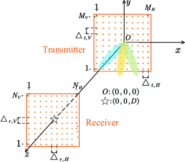
Figure 1: A UPA-based XL-MIMO system with each antenna element being a sizeless point antenna.

We first study the UPA-based XL-MIMO system with sizeless point antennas [26, 17]. As illustrated in Fig. 1, one transmitter and one receiver equipped with UPA-based XL-MIMO with point antennas are considered. The transmitter is located in the $x-y$ plane with its center being the origin. The number of transmitting antennas per row, the number of transmitting antennas per column, the horizontal side-length, and the vertical side-length of the transmitter are defined as $M_{H}$, $M_{V}$, $L_{t,H}$ and $L_{t,V}$, respectively. Thus, the horizontal and vertical antenna spacing for the transmitter can be denoted as $\Delta_{t,H}=L_{t,H}/M_{H}$ and $\Delta_{t,V}=L_{t,V}/M_{V}$, respectively. Also, the total number of transmitting antennas is $M=M_{V}M_{H}$. Inspired by [39], let $m\in\left\{1,\dots,M\right\}$ denote the antenna index row-by-row counted from the bottom left of the transmitter. Thus, the horizontal and vertical indices of the $m$-th transmitting antenna can be denoted as $i\left(m\right)=\mathrm{mod}\left(m-1,M_{H}\right)$ and $j\left(m\right)=\lfloor\left(m-1\right)/M_{H}\rfloor$, respectively. We denote the position of the $m$-th transmitting antenna by $\mathbf{r}_{t,m}=[-\frac{L_{t,H}}{2}+i\left(m\right)\Delta_{t,H},-\frac{L_{t,V}}{2}+j\left(m\right)\Delta_{t,V},0]^{T}\in\mathbb{R}^{3}$.

Meanwhile, for the receiver, let $N_{H}$ and $N_{V}$ denote the number of receiving antennas per row and per column, respectively. Thus, the receiver is equipped with a total of $N=N_{V}N_{H}$ antennas. $L_{r,H}$ and $L_{r,V}$ are the horizontal and vertical side-lengths of the receiver, respectively. Also, the horizontal and vertical antenna spacing for the receiver are $\Delta_{r,H}=L_{r,H}/N_{H}$ and $\Delta_{r,V}=L_{r,V}/N_{V}$, respectively. Note that the center of the receiver is located on the $z$ axis with $D$ being the distance between the centers of the transmitter and the receiver. Thus, the position of the $n$-th receiving antenna is defined as $\mathbf{r}_{r,n}=[-\frac{L_{r,H}}{2}+t\left(n\right)\Delta_{r,H},-\frac{L_{r,V}}{2}+k\left(n\right)\Delta_{r,V},D]^{T}\in\mathbb{R}^{3}$, where $t\left(n\right)=\mathrm{mod}\left(n-1,N_{H}\right)$ and $k\left(n\right)=\lfloor\left(n-1\right)/N_{H}\rfloor$ are the horizontal and vertical indices of the $n$-th receiving antenna, respectively, with $n\in\left\{1,\dots,N\right\}$.

II-B Channel Model

In this paper, we investigate two types of Green’s function-based channel models: scalar Green’s function-based and dyadic Green’s function-based channel models [4, 33], which are efficient to describe near-field EM wave characteristics.

II-B1 Scalar Green’s Function-Based Channel Model

For this channel model, the channel matrix between the transmitter and the receiver $\mathbf{H}_{S}\in\mathbb{C}^{N\times M}$ is generated based on the scalar Green’s function. Note that the scalar Green’s function between an arbitrary receiving point $\mathbf{r}\in\mathbb{R}^{3}$ and an arbitrary transmitting point $\mathbf{s}\in\mathbb{R}^{3}$ can be denoted as [33, 35]

$$G\left(\mathbf{r},\mathbf{s}\right)=\frac{1}{4\pi}\frac{\exp\left(-j\kappa_{0}\left|\mathbf{r}-\mathbf{s}\right|\right)}{\left|\mathbf{r}-\mathbf{s}\right|}$$ (1)

with $\kappa_{0}=2\pi/\lambda$ and $\lambda$ being the wavenumber and the wavelength, respectively. Based on (1), the channel between the $n$-th receiving antenna and $m$-th transmitting antenna $\left[\mathbf{H}_{S}\right]_{nm}=G_{nm}$ is generated by the scalar Green’s function as

$$G_{nm}=G\left(\mathbf{r}_{r,n},\mathbf{r}_{t,m}\right)=\frac{1}{4\pi}\frac{\exp\mathrm{(}-j\kappa_{0}\left|\mathbf{r}_{r,n}-\mathbf{r}_{t,m}\right|)}{\left|\mathbf{r}_{r,n}-\mathbf{r}_{t,m}\right|}.$$ (2)

II-B2 Dyadic Green’s Function-Based Channel Model

According to [33, 8], the polarization effect should be considered in near-field XL-MIMO systems and the introduction of multiple polarization can benefit the system performance. Thus, the dyadic Green’s function-based channel model is also investigated, where the multi-polarization effect is modeled. The dyadic Green’s function between a receiving point $\mathbf{r}\in\mathbb{R}^{3}$ and a transmitting point $\mathbf{s}\in\mathbb{R}^{3}$ as $\mathbf{G}\left(\mathbf{r},\mathbf{s}\right)\in\mathbb{C}^{3\times 3}$ is given as

$$\mathbf{G}\left(\mathbf{r},\mathbf{s}\right) =\frac{1}{4\pi}\left(\mathbf{I}_{3}+\frac{\nabla_{\mathbf{r}}\nabla_{\mathbf{r}}^{H}}{\kappa_{0}^{2}}\right)\frac{\exp\left(-j\kappa_{0}\left|\mathbf{r}-\mathbf{s}\right|\right)}{\left|\mathbf{r}-\mathbf{s}\right|}=\left(\mathbf{I}_{3}+\frac{\nabla_{\mathbf{r}}\nabla_{\mathbf{r}}^{H}}{\kappa_{0}^{2}}\right)G\left(\mathbf{r},\mathbf{s}\right)$$

$$=\left(1+\frac{j}{\kappa_{0}\left|\mathbf{r}-\mathbf{s}\right|}-\frac{1}{\kappa_{0}^{2}\left|\mathbf{r}-\mathbf{s}\right|^{2}}\right)\mathbf{I}_{3}G\left(\mathbf{r},\mathbf{s}\right)+\left(\frac{3}{\kappa_{0}^{2}\left|\mathbf{r}-\mathbf{s}\right|^{2}}-\frac{3j}{\kappa_{0}\left|\mathbf{r}-\mathbf{s}\right|}-1\right)\vec{\mathbf{a}}_{rs}\vec{\mathbf{a}}_{rs}G\left(\mathbf{r},\mathbf{s}\right),$$ (3)

where $\vec{\mathbf{a}}_{rs}=\left(\mathbf{r}-\mathbf{s}\right)/\left|\mathbf{r}-\mathbf{s}\right|$ is a unit direction vector. It is worth noting that the dyadic Green’s function, denoted as $\mathbf{G}\in\mathbb{C}^{3\times 3}$, can be expressed in a matrix form

$$\mathbf{G}=\left[\begin{matrix}G^{xx}&G^{xy}&G^{xz}\\ G^{yx}&G^{yy}&G^{yz}\\ G^{zx}&G^{zy}&G^{zz}\\ \end{matrix}\right],$$ (4)

where $G^{pq}\in\mathbb{C}$ is the scalar Green’s function between the polarization direction $p$ of the receiving point and the polarization direction $q$ of the transmitting point with $p,q\in\left\{x,y,z\right\}$.

According to (II-B2), the dyadic Green’s function between the $n$-th receiving antenna and the $m$-th transmitting antenna can be represented as

$$\mathbf{G}\left(\mathbf{r}_{r,n},\mathbf{r}_{t,m}\right)\!=\!\frac{1}{4\pi}\left(\mathbf{I}_{3}+\frac{\nabla_{\mathbf{r}_{r,n}}\nabla_{\mathbf{r}_{r,n}}^{H}}{\kappa_{0}^{2}}\right)G\left(\mathbf{r}_{r,n},\mathbf{r}_{t,m}\right),$$ (5)

where $G\left(\mathbf{r}_{r,n},\mathbf{r}_{t,m}\right)$ is given in (2). Based on (II-B2) and (4), the dyadic Green’s function-based channel matrix between the transmitter and the receiver can be denoted as

$$\mathbf{H}_{D}=\left[\begin{matrix}\mathbf{H}^{xx}&\mathbf{H}^{xy}&\mathbf{H}^{xz}\\ \mathbf{H}^{yx}&\mathbf{H}^{yy}&\mathbf{H}^{yz}\\ \mathbf{H}^{zx}&\mathbf{H}^{zy}&\mathbf{H}^{zz}\\ \end{matrix}\right]\in\mathbb{C}^{3N\times 3M},$$ (6)

where $\mathbf{H}^{pq}\in\mathbb{C}^{N\times M}$ is the Green’s function-based channel between the $p$ polarization direction of the receiver with $N$ antennas and the $q$ polarization direction of the transmitter with $M$ antennas. Note that the $(n,m)$-th element of $\mathbf{H}^{pq}$ is the $(p,q)$-th element of $\mathbf{G}\left(\mathbf{r}_{r,n},\mathbf{r}_{t,m}\right)$, i.e., $\left[\mathbf{H}^{pq}\right]_{nm}=G_{nm}^{pq}$.

II-C EDoF Performance Analysis

In this subsection, we analyze the EDoF performance for the UPA-based XL-MIMO system with point antennas over the scalar or dyadic Green’s function-based channels, which can provide the basis for the analysis framework for other XL-MIMO designs. Similar results have also been derived in [33], so we introduce them in a brief manner. More importantly, we compute EDoF expressions over the scalar Green’s function-based channel in the closed-form.

II-C1 Scalar Green’s function-based Channel

Based on the channel as shown in (2), we can obtain the scalar Green’s function-based channel correlation matrix $\mathbf{R}_{S}=\mathbf{H}_{S}^{H}\mathbf{H}_{S}\in\mathbb{C}^{M\times M}$. Then, the EDoF $\varepsilon_{S}$ is approximately calculated as

$$\varepsilon_{S}=\frac{\mathrm{tr}^{2}\left(\mathbf{R}_{S}\right)}{\left\|\mathbf{R}_{S}\right\|_{\mathrm{F}}^{2}}.$$ (7)

Proof:

The derivation of (7) is given in Appendix B. ∎

Terms in (7) can be expanded as

$$\begin{cases}\mathrm{tr}\left(\mathbf{R}_{S}\right)=\sum_{m=1}^{M}{\sum_{n=1}^{N}{\left[\mathbf{R}_{S}\right]_{mm}^{2}}}=\sum_{m=1}^{M}{\sum_{n=1}^{N}{\left|G_{nm}\right|^{2}}}\\ \left\|\mathbf{R}_{S}\right\|_{\mathrm{F}}^{2}=\sum_{m_{1}=1}^{M}{\sum_{m_{2}=1}^{N}{\left[\mathbf{R}_{S}\right]_{m_{1}m_{2}}^{2}}}=\sum_{m_{1}=1}^{M}{\sum_{m_{2}=1}^{N}{\left|\sum_{n=1}^{N}{G_{nm_{1}}^{*}G_{nm_{2}}}\right|^{2}}},\\ \end{cases}$$ (8)

where $\left[\mathbf{R}_{S}\right]_{m_{1}m_{2}}=\sum_{n=1}^{N}{G_{nm_{1}}^{*}G_{nm_{2}}}$ is the $m_{1}m_{2}$-th element of $\mathbf{R}_{S}$ with $m_{1},m_{2}\in\left\{1,\dots,M\right\}$. As shown in (8), $\mathrm{tr}\left(\mathbf{R}_{S}\right)$ is the overall channel power of the system. Based on (8), (7) can be computed in the closed-form as in the following theorem.

Theorem 1.

For the UPA-based XL-MIMO system over the scalar Green’s function-based channel, the EDoF in (7) can be computed in closed-form as

$$\varepsilon_{S}=\frac{D^{4}\left|\sum_{m=1}^{M}{\sum_{n=1}^{N}{\frac{1}{D^{2}+(-\frac{L_{r,H}}{2}+t(n)\Delta_{r,H}+\frac{L_{t,H}}{2}-i(m)\Delta_{t,H})^{2}+(-\frac{L_{r,V}}{2}+\Delta_{r,V}k\left(n\right)+\frac{L_{t,V}}{2}-j\left(m\right)\Delta_{t,V})^{2}}}}\right|^{2}}{\sum_{m_{1}=1}^{M}{\sum_{m_{2}=1}^{M}{\left|\sum_{n=1}^{N}{e^{-j\frac{\kappa_{0}}{D}[\Delta_{t,H}(i(m_{1})-i(m_{2}))(-\frac{L_{r,H}}{2}+t(n)\Delta_{r,H})+(-\frac{L_{r,V}}{2}+\Delta_{r,V}k(n))(j(m_{1})-j(m_{2}))\Delta_{t,V}]}}\right|^{2}}}}.$$ (9)

Proof:

The proof of Theorem 1 is given in Appendix C. ∎

II-C2 Dyadic Green’s function-based Channel

Similar to that of the scalar Green’s function, the EDoF for the UPA-based XL-MIMO system over the dyadic Green’s function-based channel can be approximately computed as

$$\varepsilon_{D}=\frac{\mathrm{tr}^{2}\left(\mathbf{R}_{D}\right)}{\left\|\mathbf{R}_{D}\right\|_{\mathrm{F}}^{2}},$$ (10)

where $\mathbf{R}_{D}=\mathbf{H}_{D}^{H}\mathbf{H}_{D}\in\mathbb{C}^{3M\times 3M}$ is the dyadic Green’s function-based channel correlation matrix.

Remark 1.

The channel in (6) embraces full triple polarization, constructed by the $x,y,z$ polarization directions of the transceiver. The double and single polarized channel can also be obtained from (6). Unless otherwise specified, the channel with double polarization includes $x$ and $y$ polarization of the transceiver, i.e.,

$$\mathbf{H}_{D,2}=\left[\begin{matrix}\mathbf{H}^{xx}&\mathbf{H}^{xy}\\ \mathbf{H}^{yx}&\mathbf{H}^{yy}\\ \end{matrix}\right]\in\mathbb{C}^{2N\times 2M}.$$ (11)

For the single polarized channel, only $x$ polarization direction of the transceiver is impinged, i.e., $\mathbf{H}_{D,1}=\left[\mathbf{H}^{xx}\right]\in\mathbb{C}^{N\times M}$. When only the single polarization is considered, the dyadic Green’s function-based channel is boiled down into the scalar Green’s function-based channel except with some additional coefficients. Note that the EDoF for the UPA-based XL-MIMO system over the double or single polarized channel can be derived by substituting the double polarized channel $\mathbf{H}_{D,2}$ and the single polarized channel $\mathbf{H}_{D,1}$ into (10).

III 2D CAP Plane-Based XL-MIMO

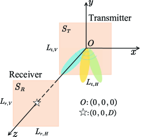
Figure 2: A 2D CAP plane-based XL-MIMO system.

III-A System Model

In this section, we study the 2D CAP plane-based XL-MIMO system as illustrated in Fig. III, where a single transmitter and a single receiver are considered. Note that the transmitter is located on the $x-y$ plane with its center being the origin. The receiver is parallel to the transmitter with its center located in $(0,0,D)$. For the transmitter, the horizontal and the vertical side-lengths are $L_{t,H}$ and $L_{t,V}$, respectively. The horizontal and vertical side-lengths for the receiver are $L_{r,H}$ and $L_{r,V}$, respectively. Let $S_{T}$ and $S_{R}$ denote the transmitting and receiving regions, respectively. We also study the scalar and dyadic Green’s function-based channels for the 2D CAP plane-based XL-MIMO system are also studied. Note that the CAP plane has the continuous aperture. For a certain transmitting point $\mathbf{r}_{t}\in\mathbb{R}^{3}$ in a continuous transmitting region $S_{T}$ and a certain receiving point $\mathbf{r}_{r}\in\mathbb{R}^{3}$ in a continuous receiving region $S_{R}$, the scalar Green’s function-based channel $G\left(\mathbf{r}_{r},\mathbf{r}_{t}\right)$ and dyadic Green’s function-based channel $\mathbf{G}\left(\mathbf{r}_{r},\mathbf{r}_{t}\right)\in\mathbb{C}^{3\times 3}$ are

$$G\left(\mathbf{r}_{r},\mathbf{r}_{t}\right) =\frac{1}{4\pi}\frac{\exp\left(-j\kappa_{0}\left|\mathbf{r}_{r}-\mathbf{r}_{t}\right|\right)}{\left|\mathbf{r}_{r}-\mathbf{r}_{t}\right|},$$ (12)

$$\mathbf{G}\left(\mathbf{r}_{r},\mathbf{r}_{t}\right) =\frac{1}{4\pi}\left(\mathbf{I}_{3}+\frac{\nabla_{\mathbf{r}_{r}}\nabla_{\mathbf{r}_{r}}^{H}}{\kappa_{0}^{2}}\right)G\left(\mathbf{r}_{r},\mathbf{r}_{t}\right).$$ (13)

Remark 2.

Similar to the scenario with the UPA-based XL-MIMO system, the double and single polarized channels for the 2D CAP plane-based XL-MIMO system can be built over the $x,y$ polarization directions and only the $x$ polarization direction, respectively. The double and single polarized channel can be derived from the full polarized channel defined in (13), by extracting $x,y$ polarized components and only $x$ polarized component from $\mathbf{G}\left(\mathbf{r}_{r},\mathbf{r}_{t}\right)$, respectively.

III-B EDoF Performance Analysis

The EDoF performance for the 2D CAP plane-based XL-MIMO system over the scalar or dyadic Green’s function-based channel is studied.

III-B1 Scalar Green’s function-based Channel

According to the methods in [35, 34, 36], we first define the auto-correlation kernel to describe the correlation characteristic for two arbitrary transmitting points $\mathbf{r}_{t}\in S_{T}$ and $\mathbf{r}_{t^{\prime}}\in S_{T}$ as

$$K(\mathbf{r}_{t},\mathbf{r}_{t^{\prime}})=\int_{S_{R}}{G^{*}\left(\mathbf{r}_{r},\mathbf{r}_{t}\right)G\left(\mathbf{r}_{r},\mathbf{r}_{t^{\prime}}\right)}d\mathbf{r}_{r}.$$ (14)

With the aid of the asymptotic analysis by letting $M\rightarrow\infty$, $N\rightarrow\infty$ to (7) with an invariant physical size, we can derive the EDoF for the 2D CAP plane-based XL-MIMO system over the scalar Green’s function-based channel as follows.

Corollary 1.

The EDoF for the 2D CAP plane-based XL-MIMO system over the scalar Green’s function-based channel can be calculated as

$$\varPsi_{S}=\frac{\left(\int_{S_{T}}{\int_{S_{R}}{\left|G\left(\mathbf{r}_{r},\mathbf{r}_{t}\right)\right|^{2}}d\mathbf{r}_{r}}d\mathbf{r}_{t}\right)^{2}}{\int_{S_{T}}{\int_{S_{T}}{\left|K(\mathbf{r}_{t},\mathbf{r}_{t^{\prime}})\right|^{2}}d}\mathbf{r}_{t}d\mathbf{r}_{t^{\prime}}}.$$ (15)

Proof:

The proof is provided in Appendix D. ∎

Remark 3.

Note that $\int_{S_{T}}{\int_{S_{R}}{\left|G\left(\mathbf{r}_{r},\mathbf{r}_{t}\right)\right|^{2}}d\mathbf{r}_{r}}d\mathbf{r}_{t}$ and ${\int_{S_{T}}{\int_{S_{T}}{\left|K(\mathbf{r}_{t},\mathbf{r}_{t^{\prime}})\right|^{2}}d}\mathbf{r}_{t}d\mathbf{r}_{t^{\prime}}}$ denote the overall channel gain across the transmitting and receiving regions and the overall power of the correlation kernel function $K(\mathbf{r}_{t},\mathbf{r}_{t^{\prime}})$ across the transmitting region.

When considering the scalar Green’s function-based channel, the EDoF for the 2D CAP plane-based XL-MIMO system can be computed in closed-form as in the following theorem.

Theorem 2.

The EDoF for the 2D CAP plane-based XL-MIMO system over the scalar Green’s function-based channel can be approximately calculated in closed-form as

$$\varPsi_{S,\mathrm{c}}=\frac{\gamma^{2}}{\xi},$$ (16)

where $\gamma$ is given as

$$\gamma =\mu_{0}\frac{2L_{t,H}L_{r,H}}{L_{H,\max}}T\left(\frac{\left|L_{t,H}-L_{r,H}\right|}{2}\right)+\mu_{0}\left(L_{t,H}+L_{r,H}\right)T\left(\frac{L_{t,H}+L_{r,H}}{2}\right)$$

$$-\mu_{0}\left(L_{t,H}+L_{r,H}\right)T\left(\frac{\left|L_{t,H}-L_{r,H}\right|}{2}\right)-2\mu_{0}Q\left(\frac{L_{t,H}+L_{r,H}}{2}\right)+2\mu_{0}Q\left(\frac{\left|L_{t,H}-L_{r,H}\right|}{2}\right)$$ (17)

with $\mu_{0}=\left(1/4\pi\right)^{2}$ and $L_{H,\max}=\max\left\{L_{t,H},L_{r,H}\right\}$. Note that $T\left(x\right)$ is

$$T\left(x\right) =\frac{2L_{t,V}L_{r,V}}{D}\mathrm{arc}\tan\frac{x}{D}+x\ln\left(\frac{\mu_{1}+4x^{2}}{\mu_{2}+4x^{2}}\right)$$ (18)

$$+\sqrt{\mu_{1}}\mathrm{arc}\tan\frac{2x}{\sqrt{\mu_{1}}}-\sqrt{\mu_{2}}\mathrm{arc}\tan\frac{2x}{\sqrt{\mu_{2}}},$$

where $\mu_{1}=\left(L_{t,V}-L_{r,V}\right)^{2}+4D^{2}$ and $\mu_{2}=\left(L_{t,V}+L_{r,V}\right)^{2}+4D^{2}$. As for $Q\left(x\right)$, we have

$$Q\left(x\right) =L_{t,V}L_{r,V}\ln\left(D^{2}+x^{2}\right)+\frac{4x^{2}+\mu_{1}}{8}\ln\left(\mu_{1}+4x^{2}\right)$$ (19)

$$-\frac{4x^{2}+\mu_{2}}{8}\ln\left(\mu_{2}+4x^{2}\right).$$

As for $\xi$, we have

$$\xi =\frac{4\mu_{3}\varphi L_{t,H}^{2}L_{t,V}^{2}}{D^{2}\left(4D^{2}+L_{t,H}^{2}\right)}+\frac{2\mu_{3}\varphi L_{t,H}L_{t,V}^{2}}{D^{3}}\mathrm{arc}\tan\frac{L_{t,H}}{2D}$$ (20)

$$+\frac{16\mu_{3}\varphi L_{t,V}^{2}}{4D^{2}+L_{t,H}^{2}}-\frac{4\mu_{3}\varphi L_{t,V}^{2}}{D^{2}}$$

where $\mu_{3}=\left(\mu_{0}L_{r,V}L_{r,H}\right)^{2}$ and $\varphi$ is the phase-related coefficient, which is computed as

$$\varphi\!=\!\frac{1}{N_{s}^{2}M_{s}^{2}}\sum_{o=1}^{M_{s}}{\sum_{u=1}^{M_{s}}{|\!\!\sum_{k^{\prime}=1}^{N_{s}}\!{\exp\left(j\kappa_{0}d_{k^{\prime}o}\right)\exp\left(-j\kappa_{0}d_{k^{\prime}u}^{\prime}\right)}|^{2}}},$$ (21)

where $d_{k^{\prime}o}=\left|\mathbf{r}_{r,k^{\prime}}-\mathbf{r}_{t,o}\right|$ and $d_{k^{\prime}u}^{\prime}=\left|\mathbf{r}_{r,k^{\prime}}-\mathbf{r}_{t^{\prime},u}\right|$ are the distances between the $k^{\prime}$-th uniformly sampled receiving point and the $o$-th or $u$-th uniformly sampled transmitting points, respectively, with $\mathbf{r}_{r,k^{\prime}}\in S_{R}$, $\left\{\mathbf{r}_{t,o},\mathbf{r}_{t^{\prime},u}\right\}\in S_{T}$, $\left\{o,u\right\}=\left\{1,\dots,M_{s}\right\}$, $k^{\prime}=\left\{1,\dots,N_{s}\right\}$. $M_{s}$ is the number of uniformly sampled transmitting points, and $N_{s}$ is the number of uniformly sampled receiving points.

Proof:

The detailed proof is provided in Appendix E. ∎

Remark 4.

As observed in Theorem 2, the EDoF performance for 2D CAP plane-based XL-MIMO systems is determined by the physical size of the transceiver, transmitting distance, and carrier frequency (or the wavenumber). Meanwhile, as shown in (2), the overall channel gain $\int_{S_{T}}{\int_{S_{R}}{\left|G\left(\mathbf{r}_{r},\mathbf{r}_{t}\right)\right|^{2}}d\mathbf{r}_{r}}d\mathbf{r}_{t}$ depends only on the physical size and transmitting distance.

III-B2 Dyadic Green’s function-based Channel

To compute the EDoF performance for the 2D CAP plane-based XL-MIMO system over the dyadic Green’s function-based channel, we define the polarized auto-correlation kernel function over a specific polarization direction pair $\left\{p,q\right\}\in\left\{1,2,3\right\}$ as

$$\hat{K}(\mathbf{r}_{t},\mathbf{r}_{t^{\prime}},p,q)\!=\!\sum_{l=1}^{3}{\int_{S_{R}}{\!}\!\left[G^{lp}\left(\mathbf{r}_{r},\mathbf{r}_{t}\right)\right]^{*}G^{lq}\left(\mathbf{r}_{r},\mathbf{r}_{t^{\prime}}\right)d\mathbf{r}_{r}},$$ (22)

where the polarization subscripts are represented, for simplicity, as $x\rightarrow 1$, $y\rightarrow 2$, and $z\rightarrow 3$, respectively. Besides, $G^{lp}\left(\mathbf{r}_{r},\mathbf{r}_{t}\right)$ denotes the $(l,p)$-th element of $\mathbf{G}\left(\mathbf{r}_{r},\mathbf{r}_{t}\right)$ as given in (13). Based on the asymptotic analysis by letting $M\rightarrow\infty$, $N\rightarrow\infty$ to (10) with an invariant physical size, we derive the EDoF for the 2D CAP plane-based XL-MIMO over the dyadic Green’s function-based channel as in the following corollary.

Corollary 2.

The EDoF for the 2D CAP plane-based XL-MIMO system over the dyadic Green’s function-based channel can be calculated as

$$\varPsi_{D}=\frac{\left(\sum_{l=1}^{3}{\sum_{p=1}^{3}{\int_{S_{T}}{\int_{S_{R}}{\left|G^{lp}\left(\mathbf{r}_{r},\mathbf{r}_{t}\right)\right|^{2}d\mathbf{r}_{r}}d\mathbf{r}_{t}}}}\right)^{2}}{\sum_{p=1}^{3}{\sum_{q=1}^{3}{\int_{S_{T}}{\int_{S_{T}}{\left|\hat{K}(\mathbf{r}_{t},\mathbf{r}_{t^{\prime}},p,q)\right|}^{2}d}\mathbf{r}_{t}d\mathbf{r}_{t^{\prime}}}}}.$$ (23)

Proof:

The detailed proof can be found in [36] and is therefore omitted. ∎

Remark 5.

Note that the EDoF computation in Corollary 2 includes full triple polarization. However, for the double or single polarized channel as discussed in Remark 1, the EDoF performance can also be studied based on the analysis framework in Corollary 2. It is worth noticing that the EDoF performance analysis framework in Corollary 2 holds for the channel with arbitrary numbers of polarization. We can compute the EDoF for the 2D CAP plane-based over the channel with arbitrary numbers of polarization as

$$\varPsi_{D}=\frac{\left(\sum_{l=1}^{N_{p}}{\sum_{p=1}^{N_{p}}{\int_{S_{T}}{\int_{S_{R}}{\left|G^{lp}\left(\mathbf{r}_{r},\mathbf{r}_{t}\right)\right|^{2}d\mathbf{r}_{r}}d\mathbf{r}_{t}}}}\right)^{2}}{\sum_{p=1}^{N_{p}}{\sum_{q=1}^{N_{p}}{\int_{S_{T}}{\int_{S_{T}}{\left|\hat{K}(\mathbf{r}_{t},\mathbf{r}_{t^{\prime}},p,q)\right|^{2}}d}\mathbf{r}_{t}d\mathbf{r}_{t^{\prime}}}}},$$ (24)

where $\hat{K}(\mathbf{r}_{t},\mathbf{r}_{t^{\prime}},p,q)\!=\!\sum_{l=1}^{N_{p}}{\int_{S_{R}}{\!}\!\left[G^{lp}\left(\mathbf{r}_{r},\mathbf{r}_{t}\right)\right]^{*}G^{lq}\left(\mathbf{r}_{r},\mathbf{r}_{t^{\prime}}\right)d\mathbf{r}_{r}}$ and $N_{p}=\left\{1,2,3\right\}$ is the number of channel polarization. When $N_{p}=1$, (24) converts to (15) over the scalar Green’s function-based channel.

IV Other XL-MIMO Hardware Designs

In this section, we introduce the EDoF performance analysis framework for other XL-MIMO hardware designs, UPA-based XL-MIMO with patch antennas and 1D XL-MIMO designs.

IV-A UPA-Based XL-MIMO with Patch Antennas

The UPA-based XL-MIMO investigated in Section II views each antenna element as a sizeless point antenna. Another practical UPA-based XL-MIMO design is to regard each antenna element as a patch antenna with a certain size and continuous aperture in each antenna element [4, 18], as illustrated in Fig. IV. For this UPA-based XL-MIMO design with patch antennas, across each antenna element, the EM wave should be captured with the aid of exact integrals due to the continuous characteristic for each element. We assume that the physical sizes of the transmitting and receiving patch antenna element can be denoted as $A_{t,H}\times A_{t,V}$ and $A_{r,H}\times A_{r,V}$, respectively, where $A_{t,H}$, $A_{t,V}$, $A_{r,H}$, and $A_{r,V}$ denote the horizontal or vertical element side-length of the transmitting antenna element and the horizontal or vertical element side length of the receiving antenna element, respectively. Other parameter definitions are similar to those of the UPA-based XL-MIMO system in Section II. Moreover, we denote the transmitting region and the receiving region as $V_{T}=\left\{V_{T,m}:m=1,\dots,M\right\}$ and $V_{R}=\left\{V_{R,n}:n=1,\dots,N\right\}$, where $V_{T,m}$ and $V_{R,n}$ are the regions of the $m$-th transmitting patch antenna and the $n$-th receiving patch antenna, respectively, defined as

$$V_{T,m}=\{(x_{t}^{m},y_{t}^{m},0)\in\mathbb{R}^{3}:\{\mathbf{r}_{t,m}\left(1\right)-\frac{A_{t,H}}{2}\leqslant x_{t}^{m}\leqslant\mathbf{r}_{t,m}\left(1\right)+\frac{A_{t,H}}{2};\mathbf{r}_{t,m}\left(2\right)-\frac{A_{t,V}}{2}\leqslant y_{t}^{m}\leqslant\mathbf{r}_{t,m}\left(2\right)+\frac{A_{t,V}}{2}\}\}$$

$$V_{R,n}=\{(x_{r}^{n},y_{r}^{n},D)\in\mathbb{R}^{2}:\{\mathbf{r}_{r,n}\left(1\right)-\frac{A_{r,H}}{2}\leqslant x_{r}^{n}\leqslant\mathbf{r}_{r,n}\left(1\right)+\frac{A_{r,H}}{2};\mathbf{r}_{r,n}\left(2\right)-\frac{A_{r,V}}{2}\leqslant y_{r}^{n}\leqslant\mathbf{r}_{r,n}\left(2\right)+\frac{A_{r,V}}{2}\}\}$$ (25)

with $\mathbf{r}_{t,m}$ and $\mathbf{r}_{r,n}$ being the coordinates of centers of the $m$-th transmitting and the $n$-th receiving patch antennas, respectively. Note that $\mathbf{r}_{t,m}$ and $\mathbf{r}_{r,n}$ are also the coordinates of the $m$-th transmitting and the $n$-th receiving point antennas, respectively, as defined in Section II.

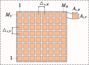
Figure 3: An illustration of the transmitter equipped with UPA-based XL-MIMO with patch antennas.

When computing the UPA-based XL-MIMO system with patch antennas, as discussed above, exact integrals across each patch antenna element should be computed. The auto-correlation kernel function $K(\mathbf{r}_{t},\mathbf{r}_{t^{\prime}})$ can be derived from (14), by considering ${V_{T}}$ and $V_{R}$, as

$$K(\mathbf{r}_{t},\mathbf{r}_{t^{\prime}})=\int_{V_{R}}{G^{*}\left(\mathbf{r}_{r},\mathbf{r}_{t}\right)G\left(\mathbf{r}_{r},\mathbf{r}_{t^{\prime}}\right)}d\mathbf{r}_{r}=\sum_{n=1}^{N}{[\int_{V_{R,n}}{G^{*}(\mathbf{r}_{r}^{n},\mathbf{r}_{t})G(\mathbf{r}_{r}^{n},\mathbf{r}_{t^{\prime}})}d\mathbf{r}_{r}^{n}]},$$ (26)

where $\mathbf{r}_{r}^{n}=(x_{r}^{n},y_{r}^{n},D)\in V_{R,n}$ and $G(\mathbf{r}_{r}^{n},\mathbf{r}_{t})$ can be derived as in (12). Based on the above definitions and motivated by Corollary 1, we derive the EDoF analysis framework for the UPA-based XL-MIMO system with patch antennas over the scalar Green’s function-based channel in the following.

Corollary 3.

For the UPA-based XL-MIMO system with patch antennas over the scalar Green’s function-based channel, the EDoF $\psi_{S}$ can be computed as

$$\psi_{S}=\frac{\left(\int_{V_{T}}{\int_{V_{R}}{\left|G\left(\mathbf{r}_{r},\mathbf{r}_{t}\right)\right|^{2}}d\mathbf{r}_{r}}d\mathbf{r}_{t}\right)^{2}}{\int_{V_{T}}{\int_{V_{T}}{\left|K(\mathbf{r}_{t},\mathbf{r}_{t^{\prime}})\right|^{2}}d}\mathbf{r}_{t}d\mathbf{r}_{t^{\prime}}}.$$ (27)

Note that (27) can be further written as

$$\psi_{S}=\frac{\left\{\sum_{n=1}^{N}{\sum_{m=1}^{M}{\left[\int_{V_{T,m}}{\int_{V_{R,n}}{\left|G\left(\mathbf{r}_{r}^{n},\mathbf{r}_{t}^{m}\right)\right|^{2}}}d\mathbf{r}_{r}^{n}d\mathbf{r}_{t}^{m}\right]}}\right\}^{2}}{\sum_{m_{1}=1}^{M}{\sum_{m_{2}=1}^{M}{\int_{V_{T,m_{1}}}{\int_{V_{T,m_{2}}}{\left|\sum_{n=1}^{N}{\left[\int_{V_{R,n}}{G^{*}\left(\mathbf{r}_{r}^{n},\mathbf{r}_{t}^{m_{1}}\right)G\left(\mathbf{r}_{r}^{n},\mathbf{r}_{t^{\prime}}^{m_{2}}\right)}d\mathbf{r}_{r}^{n}\right]}\right|^{2}}}d\mathbf{r}_{t}^{m_{1}}d\mathbf{r}_{t^{\prime}}^{m_{2}}}}}$$ (28)

Proof:

This corollary can be easily derived by substituting $V_{T}$ and $V_{R}$ into (15). ∎

Similarly, based on (22), the polarized auto-correlation kernel function for the UPA-based XL-MIMO system with patch antennas can be defined as

$$\hat{K}(\mathbf{r}_{t},\mathbf{r}_{t^{\prime}},p,q)\!=\!\sum_{l=1}^{3}{\int_{V_{R}}{\!}\![G^{lp}(\mathbf{r}_{r},\mathbf{r}_{t})]^{*}G^{lq}(\mathbf{r}_{r},\mathbf{r}_{t^{\prime}})d\mathbf{r}_{r}}=\sum_{n=1}^{N}{\sum_{l=1}^{3}{[\int_{V_{R,n}}{\!}\![G^{lp}(\mathbf{r}_{r}^{n},\mathbf{r}_{t})]^{*}G^{lq}(\mathbf{r}_{r}^{n},\mathbf{r}_{t^{\prime}})d\mathbf{r}_{r}^{n}]}}.$$ (29)

Thus, we can derive the EDoF performance over the dyadic Green’s function-based channel as in the following corollary.

Corollary 4.

For the UPA-based XL-MIMO system with patch antennas over the dyadic Green’s function-based channel, the EDoF $\psi_{D}$ can be computed as

$$\psi_{D}=\frac{\left(\sum_{l=1}^{3}{\sum_{p=1}^{3}{\int_{V_{T}}{\int_{V_{R}}{\left|G^{lp}\left(\mathbf{r}_{r},\mathbf{r}_{t}\right)\right|^{2}d\mathbf{r}_{r}}d\mathbf{r}_{t}}}}\right)^{2}}{\sum_{p=1}^{3}{\sum_{q=1}^{3}{\int_{V_{T}}{\int_{V_{T}}{\left|\hat{K}(\mathbf{r}_{t},\mathbf{r}_{t^{\prime}},p,q)\right|^{2}}d}\mathbf{r}_{t}d\mathbf{r}_{t^{\prime}}}}}.$$ (30)

Besides, (30) can be further expanded as

$$\psi_{D}=\frac{\left(\sum\nolimits_{n=1}^{N}{\sum\nolimits_{m=1}^{M}{\sum\nolimits_{l=1}^{3}{\sum\nolimits_{p=1}^{3}{\left[\int_{V_{T,m}}{\int_{V_{R,n}}{\left|G^{lp}\left(\mathbf{r}_{r}^{n},\mathbf{r}_{t}^{m}\right)\right|^{2}}}d\mathbf{r}_{r}^{n}d\mathbf{r}_{t}^{m}\right]}}}}\right)^{2}}{\sum\nolimits_{m_{1}=1}^{M}{\sum\nolimits_{m_{2}=1}^{M}{\sum\nolimits_{p=1}^{3}{\sum\nolimits_{q=1}^{3}{\int_{V_{T,m_{1}}}{\int_{V_{T,m_{2}}}{\left|\sum\nolimits_{n=1}^{N}{\sum\nolimits_{l=1}^{3}{\left[\int_{V_{R,n}}{\!}\!\left[G^{lp}\left(\mathbf{r}_{r}^{n},\mathbf{r}_{t}^{m_{1}}\right)\right]^{*}G^{lq}\left(\mathbf{r}_{r}^{n},\mathbf{r}_{t^{\prime}}^{m_{2}}\right)d\mathbf{r}_{r}^{n}\right]}}\right|^{2}d\mathbf{r}_{t}^{m_{1}}d\mathbf{r}_{t^{\prime}}^{m_{2}}}}}}}}}.$$ (31)

Proof:

We can easily prove this corollary by substituting $V_{T}$ and $V_{R}$ into (23). ∎

Remark 6.

From a mathematical perspective, Corollary 3 and Corollary 4 provide an important unified analytical framework due to the flexible configuration of the patch antenna element. When the side-lengths of each patch antenna element be infinitesimal, that is $A_{\left\{t,r\right\},\left\{V,H\right\}}\rightarrow 0$, or assuming that only the center of each patch antenna element is impinged for transmitting/receiving EM wave, that is $V_{T,m}=\mathbf{r}_{t,m}$ and $V_{R,n}=\mathbf{r}_{r,n}$, Corollary 3 and Corollary 4 are equivalent to (7) and (10) for UPA-based XL-MIMO systems with point antennas, respectively. Moreover, when the side-lengths of each patch antenna element equal to the antenna spacing in the respective directions, that is $A_{t,\left\{H,V\right\}}=\Delta_{t,\left\{H,V\right\}}$ and $A_{r,\left\{H,V\right\}}=\Delta_{r,\left\{H,V\right\}}$, the array aperture for the UPA-based XL-MIMO with patch antennas would be continuous, and thus, Corollary 3 and Corollary 4 would covert to Corollary 1 and Corollary 2 for 2D CAP plane-based XL-MIMO, respectively.

IV-B 1D XL-MIMO Hardware Designs

The above investigated XL-MIMO hardware designs are all of the 2D characteristics. In this part, we investigate 1D XL-MIMO hardware designs, ULA-based XL-MIMO, and 1D CAP line segment-based XL-MIMO, and derive their respective EDoF performance analysis framework.

IV-B1 ULA-Based XL-MIMO

Under this hardware design, we assume that the transmitter equipped with ULA-based XL-MIMO is located on the $y$-axis with its centering coordinate being $(0,0,0)$. The side-length and the number of antennas for the transmitter can be denoted as $L_{t}$ and $M$, respectively. Besides, the receiver equipped with the ULA-based XL-MIMO embraces the side-length of $L_{r}$ and $N$ antennas. Note that the coordinates of the $m$-th transmitting antenna or $n$-th receiving antenna can be denoted as $\mathbf{r}_{t,m}=[0,-\frac{L_{t,V}}{2}+\left(m-1\right)\Delta_{t},0]^{T}\in\mathbb{R}^{3}$ and $\mathbf{r}_{r,n}=[0,-\frac{L_{r,V}}{2}+\left(n-1\right)\Delta_{r},D]^{T}\in\mathbb{R}^{3}$, respectively, where $\Delta_{t}=L_{t}/M$ and $\Delta_{r}=L_{r}/N$ are the antenna spacing for the transmitter and the receiver, respectively, with $m=1,\dots,M$ and $n=1,\dots,N$.

Similar to the UPA-based XL-MIMO system with point antennas, we can also compute the EDoF performance for the ULA-based XL-MIMO system over the scalar and dyadic Green’s function-based channel same as in (7) and (10), respectively, where applied channel matrices are derived by substituting the parameters of the ULA-based XL-MIMO system into (2) and (5), respectively. Note that, when considering the scalar Green’s function-based channel, we can compute the EDoF in closed-form as in the following theorem.

Theorem 3.

The EDoF over the scalar Green’s function-based channel can be computed in the closed-form as

$$\varepsilon_{S}\!=\!\frac{D^{4}|\sum_{m=1}^{M}{\sum_{n=1}^{N}{\frac{1}{D^{2}+[-\frac{L_{r}}{2}+\left(n-1\right)\Delta_{r}+\frac{L_{t}}{2}-(m-1)\Delta_{t}]^{2}}}}|^{2}}{\sum_{m_{1}=1}^{M}\!{\sum_{m_{2}=1}^{M}{|\sum_{n=1}^{N}\!{e^{-j\frac{\kappa_{0}}{D}[(-\frac{L_{r}}{2}+(n-1)\Delta_{r})(m_{1}-m_{2})\Delta_{t}]}}|^{2}}}}.$$ (32)

Proof:

The proof can be easily derived based on the similar method to that of Theorem 1. ∎

IV-B2 1D CAP Line Segment-Based XL-MIMO

For this design, unlike 2D CAP planes considered in Section III, we study 1D line segments with the continuous array aperture. The transmitter with the side-length of $L_{t}$ is located on the $y$ axis with its center being $(0,0,0)$. And the receiver with the side-length of $L_{r}$ is parallel to the transmitter with its center being $(0,0,D)$. Note that the EDoF performance for this design over the scalar and dyadic Green’s function-based channel can be formulated similarly to that of the 2D CAP plane-based XL-MIMO system as shown in Corollary 1 and Corollary 2, respectively, by substituting the transmitting and receiving regions of this design into these corollaries. More importantly, over the scalar Green’s function-based channel, the EDoF can also be computed in closed-form as in the following theorem.

Theorem 4.

We can compute the EDoF over the scalar Green’s function-based channel in closed-form as

$$\varPsi_{S,\mathrm{c}}=\frac{\left\{2L_{t}L_{r}-D^{2}\ln\left[\frac{\left(L_{t}+L_{r}\right)^{2}+4D^{2}}{\left(L_{t}-L_{r}\right)^{2}+4D^{2}}\right]\right\}^{2}}{\varphi\left(L_{t}L_{r}\right)^{2}},$$ (33)

where $\varphi$ is similar to the definition in (21).

Proof:

We can easily obtain this theorem based on a similar method to that of Theorem 2. ∎

Remark 7.

The capacity performance $C$ for all investigated XL-MIMO designs can be directly derived based on the studied EDoF expressions in this paper as $C=\mathrm{EDoF}\cdot\log_{2}(1+\frac{\alpha P}{\mathrm{EDoF}^{2}N_{0}})$ [37], where $\alpha$ is the overall channel gain, $P$ is the transmitting power, and $N_{0}$ is the noise power. Note that $\alpha$ can denoted as the square root of the numerator of the respective EDoF expression.

V Numerical Results

In this paper, we study the EDoF performance for XL-MIMO systems over the scalar and dyadic Green’s function-based channels. Unless otherwise specified, for the UPA-based and 2D CAP plane-based XL-MIMO system, we consider the square plane, that is $L_{t,V}=L_{t,H}$ and $L_{r,V}=L_{r,H}$. Besides, we consider that the numbers of antennas per side of the UPA are equal, that is $M_{V}=M_{H}$ and $N_{V}=N_{H}$. The carrier frequency considered in this paper is $30\,\text{GHz}$.

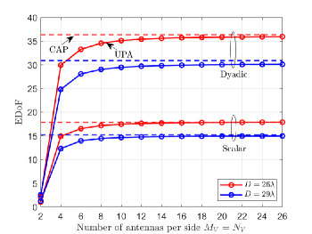
Figure 4: EDoF performance for UPA-based with point antennas and 2D CAP plane-based XL-MIMO system with $L_{t,V}=L_{r,V}=10\lambda$ over the dyadic and scalar Green’s function-based channels.

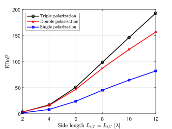
Figure 5: EDoF performance for 2D CAP plane-based XL-MIMO system against the side-length over Green’s function-based channels with different numbers of polarization with $D=6\lambda$.

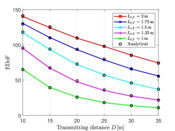
Figure 6: EDoF performance for the 2D CAP square plane-based XL-MIMO system against $D$ with different values of $L_{t,V}=L_{r,V}$ over the scalar Green’s function-based channel.

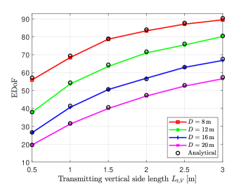
Figure 7: EDoF performance for the 2D CAP rectangle plane-based XL-MIMO system against different values of $L_{t,V}$ with $L_{t,H}=L_{r,H}=1\,\mathrm{m}$ and $L_{r,V}=1.5\,\mathrm{m}$ over the scalar Green’s function-based channel.

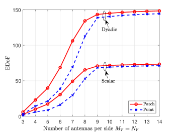
Figure 8: EDoF performance for the UPA-based XL-MIMO system with point or patch antenna elements against the number of antennas per side $M_{V}=N_{V}$ with $L_{t,V}=L_{r,V}=10\lambda$, $D=10\lambda$, and $A_{r,\left\{H,V\right\}}=A_{t,\left\{H,V\right\}}=\lambda/2$ over both the dyadic and scalar Green’s function-based channels.

In Fig. 4, we compare the EDoF performance between the UPA-based XL-MIMO system with point antennas and the 2D CAP plane-based XL-MIMO system over both the dyadic and scalar Green’s function-based channels. We can observe that as the number of antennas of the UPA increases, the EDoF performance for the UPA-based system approaches that of the CAP-based system over both the dyadic and scalar Green’s function-based channels. This observation indicates that the physical size of the XL-MIMO system imposes restrictive constraints on the EDoF performance. It is vital to observe that increasing the number of antennas in a fixed physical size may not always benefit the EDoF performance, but lead to an approximately saturated value. Besides, the dyadic Green’s function-based channel can significantly enhance the EDoF performance compared with that of the scalar Green’s function channel due to the consideration of full polarization, e.g. about $104\%$ EDoF improvement for $D=26\lambda$, highlighting the importance of utilizing the dyadic Green’s function-based channel to fully exploit the EDoF performance of XL-MIMO.

Fig. 5 evaluates the effects of polarization in channels. We consider the EDoF performance for the 2D CAP plane-based XL-MIMO system as a function of the side-length over channels with different numbers of polarization. We can observe that the triple and double polarized channels can enhance the EDoF performance compared with that of the single polarized channel, i.e., scalar Green’s function-based channel. Furthermore, with the increase of the side-length, the EDoF performance improvement for the triple polarized channel compared with that of the double and single polarized channels becomes larger, e.g. $23.2\%$ and $135.5\%$ improvement for $L_{t,V}=12\lambda$ as well as $8.6\%$ and $113.4\%$ improvement for $L_{t,V}=6\lambda$, respectively. More importantly, we observe that when the side-length is small, the EDoF performance of the triple polarized channel closely approaches the EDoF performance of the double polarized channel. This phenomenon is due to the fact that when the transmitting distance is comparable to the physical size of the system, the effect of $z$ polarization vanishes. In other words, for an XL-MIMO system with a fixed physical size, the effect of $z$ polarization would diminish and eventually vanish with the increase of the transmitting distance $D$.

Fig. 6 investigates the EDoF performance for the 2D CAP square plane-based XL-MIMO system over the scalar Green’s function-based channel. We observe that the EDoF performance benefits from the increase of the side-length or the decrease of the transmitting distance. More importantly, it can be found that markers “$\circ$” generated by the EDoF closed-form results as described in Theorem 2 match well with the curves generated by the simulation results, which validates our derived EDoF closed-form results for the 2D CAP plane-based XL-MIMO system in Theorem 2 over different values of the side-lengths and transmitting distances. In Fig. 7, we provide further validation of the EDoF closed-form results in Theorem 2. We consider the 2D CAP rectangle plane-based XL-MIMO system with transmitting rectangle planes of different shapes over the scalar Green’s function-based channel. As observed, the EDoF closed-form results, denoted by “$\circ$”, match well with the simulation results denoted by the curves, confirming the accuracy of our derived EDoF closed-form results in rectangle plane-based scenarios with varying side-lengths. Moreover, with the increase of $L_{t,V}$, the EDoF performance increases with diminishing returns, due to the performance constraint introduced by the limited physical size of the receiver, e.g. $22.3\%$ and $2.7\%$ EDoF improvement for $L_{t,V}=1\,\mathrm{m}$ compared with $L_{t,V}=0.5\,\mathrm{m}$ and $L_{t,V}=3\,\mathrm{m}$ compared with $L_{t,V}=2.5\,\mathrm{m}$, respectively, for $D=8\,\mathrm{m}$.

Fig. 8 compares the EDoF performance for the UPA-based system with point antennas and that of the UPA-based system with patch antennas. Note that the design with patch antennas can achieve better EDoF performance than the design with point antennas when the antennas are deployed in a non-dense manner, i.e., when $M_{V}=N_{V}$ are small. When the antennas are deployed non-densely, the EDoF performance for the UPA-based has not yet reached its saturated values. In such a case, patch antennas with a certain element size can efficiently capture EM waves across their element regions, resulting in better EDoF performance compared to point antennas. For instance, for the case with $M_{V}=N_{V}=7$, the scenario with patch antennas can achieve $53.7\%$ and $66.5\%$ EDoF performance improvement over the dyadic and scalar Green’s function-based channels, respectively, compared with the scenario with point antennas. However, as the number of antennas further increases, the performance gaps between the patch antenna scenario and the point antenna scenario reduce, since both the scenarios with patch antennas and point antennas would eventually reach approximately equal saturated EDoF values, limited by the physical sizes of the transmitter and the receiver.

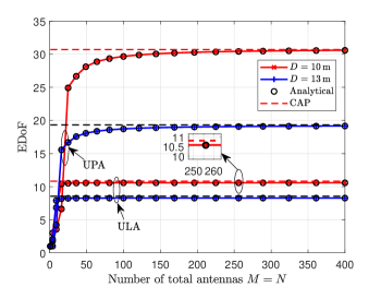
Figure 9: EDoF performance for the square UPA-based XL-MIMO system with $L_{t,V}=L_{r,V}=\sqrt{2}/2\,\mathrm{m}$ and $M_{H,V}=N_{H,V}$, and the ULA-based XL-MIMO system with $L_{t}=L_{r}=1\,\mathrm{m}$ and $M=N$ against the total number of antennas $M=N$ over the scalar Green’s function-based channel.

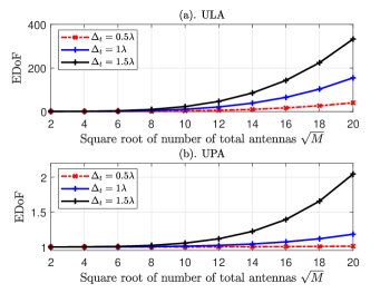
Figure 10: EDoF performance for the UPA-based XL-MIMO system with $M_{H,V}=N_{H,V}=\sqrt{M}$ and ULA-based XL-MIMO system with $M=N$ against $\sqrt{M}$ over different antenna spacing.

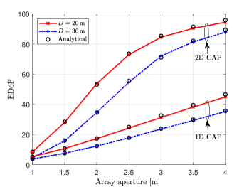
Figure 11: EDoF performance for 2D CAP plane-based and 1D CAP line segment-based XL-MIMO systems with the same array aperture size over the scalar Green’s function-based channel over different values of the array aperture size.

In Fig. 9 and Fig. 10, we compare the EDoF performance between the UPA-based XL-MIMO system with point antennas and the ULA-based XL-MIMO system over the scalar Green’s function-based channel. To ensure fairness in the comparison, it is important to establish appropriate criteria [4]. The first potential criteria is to compare the EDoF performance for the UPA-based and ULA-based systems with the same array aperture. For the ULA-based system utilizing a 1D array, the array aperture for the transmitter/receiver is the respective side-length. For the UPA-based system, which employs a 2D array, the array aperture for the transmitter/receiver is their respective length of the diagonal of the array. As observed in Fig. 9, with the same array aperture size, the UPA-based system can achieve remarkably superior EDoF performance compared with the ULA-based XL-MIMO. Indeed, with the same array aperture size, 2D spatial resources can be effectively utilized to enhance the EDoF performance. We also validate the EDoF closed-form results for the UPA-based and ULA-based XL-MIMO systems in Theorem 1 and Theorem 3, respectively. Moreover, as the number of antennas increases, the EDOF performance for both the UPA-based and ULA-based systems approaches to that of respective CAP-based systems.

Another comparison criteria is to consider the UPA-based and ULA-based with the same number of antennas. In Fig. 10, we compare the EDoF performance for the UPA-based and ULA-based systems with the same total numbers of antennas, i.e., same $M=N$, over different values of antenna spacing. We assume that $\Delta_{t,\left\{H,V\right\}}=\Delta_{r,\left\{H,V\right\}}=\Delta_{t}=\Delta_{r}$. Under this setting, the physical size of the transceiver can be adjusted according to the variations in the number of antennas. We observe from Fig. 10 that the ULA-based system can achieve significantly superior EDoF performance compared with the UPA-based system. This phenomenon is attributed to the much larger array aperture size for the ULA-based system compared with that of the UPA-based system, e.g. $6\,\mathrm{m}$ and $0.42\,\mathrm{m}$ array aperture for the ULA-based and UPA-based system with $\Delta_{t}=1.5\lambda$, respectively. Due to the 2D antenna deployment characteristic, the array aperture for the UPA-based system remains relatively small, even with a large number of antennas, such as $M=400$.

As can be observed from the above, as the number of antennas increases, the EDoF performance for discrete XL-MIMO designs, i.e., UPA-based and ULA-based designs, approaches that of their respective continuous XL-MIMO designs, i.e., 2D CAP plane-based and 1D CAP line segment-based designs, respectively. Thus, it is interesting to compare the EDoF performance between 2D CAP plane-based and 1D CAP line segment-based systems to bring a comprehensive vision of the EDoF performance of all XL-MIMO designs. It can be observed from Fig. 11 that with the same aperture size, the 2D CAP plane-based system can achieve higher EDoF performance compared to the 1D CAP line segment-based system, e.g. $109.9\%$ EDoF performance enhancement with the array aperture of $4\,\mathrm{m}$ and $D=20\,\mathrm{m}$. Moreover, we can validate the EDoF closed-form results for both the 2D CAP system and 1D CAP system derived in Theorem 2 and Theorem 4, respectively. Based on the above findings, we demonstrate that the EDoF performance is primarily constrained and determined by the physical size (array aperture) rather than the number of antennas. From the goal of higher EDoF performance, the plane-based system or the line segment-based system is advocated when designing the system with a certain length of array aperture or with a certain number of antennas. To achieve higher EDoF performance, it is recommended to apply either the plane-based system or the line segment-based system, depending on the specific requirements of the system design, such as the specific length of the array aperture or the specific number of antennas.

VI Conclusions

In this paper, we presented a comprehensive investigation of the EDoF performance analysis framework for near-field XL-MIMO systems. We studied both the discrete XL-MIMO designs, i.e., UPA-based XL-MIMO designs with point or patch antennas and ULA-based XL-MIMO design, and the continuous XL-MIMO designs, i.e. 2D CAP plane-based XL-MIMO design and 1D CAP line segment-based XL-MIMO design. Notably, scalar and dyadic Green’s function-based near-field channel models were considered. When applying the scalar channels, we derived the closed-form EDoF expressions. In numerical results, we thoroughly evaluated and compared the EDoF performance for all studied scenarios. The accuracy of the proposed closed-form results was validated through extensive simulation results. More significantly, we observed that the consideration of multiple polarization and the increase of array aperture could benefit the EDoF performance. In particular, the EDoF is constrained by the array aperture size and thus showcases saturated values as the number of antennas increases.

Appendix A Useful Results

In this appendix, we provide some useful basics, which will be applied for the computation of EDoF closed-form expressions later. For a real-valued number $x$, by applying the first-order Taylor expansion, we have

$$\sqrt{x+1}\approx 1+\frac{x}{2}.$$ (34)

Besides, we have

$$\mathrm{arc}\tan x\approx x.$$ (35)

Moreover, for two variables $x$ and $y$ approaching $0$, we have

$$x^{2}+y^{2}\approx\frac{\left(x+y\right)}{2}^{2}$$ (36)

Then, we list the indefinite integral expressions used in the following. With a constant $a$, we have

$$\int{\frac{x}{x^{2}+a^{2}}dx} =\frac{1}{2}\ln\left(x^{2}+a^{2}\right),$$ (37)

$$\int{\frac{1}{x^{2}+a^{2}}dx} =\frac{1}{a}\mathrm{arc}\tan\frac{x}{a}\,\,a>0,$$ (38)

$$\int{\ln\left(a^{2}+x^{2}\right)dx} =x\ln\left(a^{2}+x^{2}\right)-2x+2a\mathrm{arc}\tan\frac{x}{a},$$ (39)

$$\int{x\ln\left(a^{2}+x^{2}\right)dx} =\frac{x^{2}+a^{2}}{2}\ln\left(a^{2}+x^{2}\right)-\frac{1}{2}x^{2}.$$ (40)

Moreover, with constants $a$ and $b$, we have

$$\int{\frac{a}{\left(b+y^{2}\right)^{2}}}dy =\frac{ay}{2b\left(y^{2}+b\right)}+\frac{a}{2b\sqrt{b}}\mathrm{arc}\tan\left(\frac{y}{\sqrt{b}}\right),$$ (41)

$$\int{\frac{ay}{\left(b+y^{2}\right)^{2}}dy} =-\frac{a}{2\left(b+y^{2}\right)}.$$ (42)

Appendix B Proof of (7)

Note that EDoF studied in this paper is an intuitive concept, which is introduced in [37] based on the theory in [38]. In the low-SNR regime, the system capacity can be approximately computed as $C=\mathrm{EDoF}\cdot[\log_{2}(\frac{E_{b}}{N_{0}})-\log_{2}(\frac{E_{b}}{N_{0}}_{\min})]$, where ${E_{b}}/{N_{0}}$ is the SNR per bit and $[{E_{b}}/{N_{0}}]_{\min}$ is the minimum bit SNR for reliable communication. As such, $\mathrm{EDoF}$ can be computed as $\mathrm{EDoF}=\mathrm{tr}^{2}\left(\mathbf{R}\right)/\left\|\mathbf{R}\right\|_{\mathrm{F}}^{2}$ in the low-SNR regime, where $\mathbf{R}$ is the channel correlation matrix, which is in detail proven in [35, Appendix A].

More importantly, the EDoF concept defined as (7) is an approximately mathematical solution of the number of dominant sub-channels. This definition is not directly related to the number of dominant sub-channels, which is so-called $\mathrm{EDoF}_{1}$ in [32]. Note that the singular values of the channel matrix based on the spherical wave characteristics can be denoted by $\sigma_{1}\approx\sigma_{2}\approx\dots\approx\sigma_{\mathrm{EDoF}_{1}}\gg\sigma_{\mathrm{EDoF}_{1}+1}>\dots>\sigma_{\mathrm{DoF}}$ from large to small. As observed, the singular values are approximately equal before a particular threshold $\mathrm{EDoF}_{1}$ and then drop rapidly until $\mathrm{DoF}$, which is the number of total singular values. Interestingly, various experiments [32, 35] have verified that the EDoF expressions computed as (7) is a mathematical approximation of ${\mathrm{EDoF}_{1}}$ under the spherical wave based near field channel, which can be found in [32, Fig. 3] and [35, Fig. 4].

Appendix C Proof of Theorem 1

Note that $\left[\mathbf{R}_{S}\right]_{m_{1}m_{2}}=\sum_{n=1}^{N}{\frac{\exp\left(j\kappa_{0}\left(d_{nm_{1}}-d_{nm_{2}}\right)\right)}{(4\pi)^{2}d_{nm_{1}}d_{nm_{2}}}}$, where $d_{nm_{1}}=\left|\mathbf{r}_{r,n}-\mathbf{r}_{t,m_{1}}\right|$ and $d_{nm_{2}}=\left|\mathbf{r}_{r,n}-\mathbf{r}_{t,m_{2}}\right|$ are the distances between the $n$-th receiving antenna and the ${m_{1},m_{2}}$-th transmitting antenna, respectively. By applying the coordinates of the receiving and transmitting antennas defined in Section II-A and the first-order Taylor expansion as (34), we can denote $d_{nm_{1}}$ as

$$d_{nm_{1}} =\sqrt{D^{2}+(-\frac{L_{r,H}}{2}+t\left(n\right)\Delta_{r,H}+\frac{L_{t,H}}{2}-i\left(m\right)\Delta_{t,H})^{2}+(-\frac{L_{r,V}}{2}+k\left(n\right)\Delta_{r,V}+\frac{L_{t,V}}{2}-j\left(m\right)\Delta_{t,V})^{2}}$$

$$\approx D+\small{\frac{(-\frac{L_{r,H}}{2}+t\left(n\right)\Delta_{r,H}+\frac{L_{t,H}}{2}-i\left(m\right)\Delta_{t,H})^{2}+(-\frac{L_{r,V}}{2}+k\left(n\right)\Delta_{r,V}+\frac{L_{t,V}}{2}-j\left(m\right)\Delta_{t,V})^{2}}{2D}}.$$ (43)

By substituting (C) into (8), we can compute the EDoF for the UPA-based XL-MIMO system over the scalar channel in the closed-form as Theorem 1.

Appendix D Proof Corollary 3

By applying the asymptotic analysis for (8) by letting $M,N\rightarrow\infty$, $\mathrm{tr}\left(\mathbf{R}_{S}\right)$, and $\left\|\mathbf{R}_{S}\right\|_{\mathrm{F}}^{2}$ can be represented as

$$\begin{cases}\mathrm{tr}\left(\mathbf{R}_{S}\right)\rightarrow\frac{N_{H}N_{V}M_{H}M_{V}}{L_{r,H}L_{r,V}L_{t,H}L_{t,V}}\int_{S_{T}}{\int_{S_{R}}{\left|G\left(\mathbf{r}_{r},\mathbf{r}_{t}\right)\right|^{2}}d\mathbf{r}_{r}}d\mathbf{r}_{t}\\ \left\|\mathbf{R}_{S}\right\|_{\mathrm{F}}^{2}\rightarrow\left(\frac{N_{H}N_{V}M_{H}M_{V}}{L_{r,H}L_{r,V}L_{t,H}L_{t,V}}\right)^{2}\int_{S_{T}}{\int_{S_{T}}{\left|K(\mathbf{r}_{t},\mathbf{r}_{t^{\prime}})\right|^{2}}d}\mathbf{r}_{t}d\mathbf{r}_{t^{\prime}}\\ \end{cases}$$ (44)

according to the asymptotic representation $d\mathbf{r}_{r}=dx_{r}dy_{r}\rightarrow\frac{L_{r,H}L_{r,V}}{N_{H}N_{V}}$, $d\mathbf{r}_{t}=dx_{t}dy_{t}\rightarrow\frac{L_{t,H}L_{t,V}}{M_{H}M_{V}}$, and $d\mathbf{r}_{t^{\prime}}=dx_{t^{\prime}}dy_{t^{\prime}}\rightarrow\frac{L_{t,H}L_{t,V}}{M_{H}M_{V}}$ [34]. Based on the above asymptotic terms, we can derive the EDoF expressions for the CAP-based XL-MIMO system over the scalar Green’s function-based channel as shown in (15).

Appendix E Proof Theorem 2

We provide the detailed proof steps to compute the EDoF for the 2D CAP plane-based XL-MIMO system over the scalar Green’s function-based channel in a closed-form. Firstly, we start from the computation of $\gamma$. Note that we define $\gamma=\int_{S_{R}}{\int_{S_{T}}{|G(\mathbf{r}_{r},\mathbf{r}_{t})|^{2}d\mathbf{r}_{t}d\mathbf{r}_{r}}}$ as the channel power gain of the 2D CAP plane-based XL-MIMO system over the scalar Green’s function-based channel. Based on the probability theory, we can denote $\gamma$ as

$$\gamma =\int_{S_{R}}{\int_{S_{T}}{|G(\mathbf{r}_{r},\mathbf{r}_{t})|^{2}d\mathbf{r}_{t}d\mathbf{r}_{r}}}=\mu_{0}\int_{-\frac{L_{t,H}}{2}}^{\frac{L_{t,H}}{2}}{\int_{-\frac{L_{t,V}}{2}}^{\frac{L_{t,V}}{2}}{\int_{-\frac{L_{r,H}}{2}}^{\frac{L_{r,H}}{2}}{\int_{-\frac{L_{r,V}}{2}}^{\frac{L_{r,V}}{2}}{\frac{dx_{r}dy_{r}dx_{t}dy_{t}}{D^{2}+\left(x_{r}-x_{t}\right)^{2}+\left(y_{r}-y_{t}\right)^{2}}}}}}$$

$$=\mu_{0}L_{t,H}L_{r,H}L_{t,V}L_{r,V}\int_{0}^{\frac{L_{t,H}+L_{r,H}}{2}}{\int_{0}^{\frac{L_{t,V}+L_{r,V}}{2}}{\frac{f\left(x\right)g\left(y\right)dxdy}{D^{2}+x^{2}+y^{2}}}},$$ (45)

where $f\left(x\right)$ and $g\left(y\right)$ are the probability density functions (PDFs) of $x\triangleq\left|x_{t}-x_{r}\right|\in[0,\frac{L_{t,H}+L_{r,H}}{2}]$ and $y\triangleq\left|y_{t}-y_{r}\right|\in[0,\frac{L_{t,V}+L_{r,V}}{2}]$, respectively. As for the computation of PDFs, we take $f\left(x\right)$ as an example. Based on the value ranges of $x_{t}$ and $x_{r}$, we can compute the probability distribution function $F\left(x\right)$ based on the area ratio between the aimed region and the total value region. For the scenario with $L_{t,H}\geqslant L_{r,H}$, when $0\leqslant x\leqslant\frac{L_{t,H}-L_{r,H}}{2}$, we have $F\left(x\right)=\frac{2x\cdot L_{r,H}}{L_{t,H}L_{r,H}}=\frac{2x}{L_{t,H}}$. When $\frac{L_{t,H}-L_{r,H}}{2}\leqslant x\leqslant\frac{L_{t,H}+L_{r,H}}{2}$, we have $F\left(x\right)=[L_{t,H}L_{r,H}-2\times\frac{1}{2}(\frac{L_{t,H}+L_{r,H}}{2}-x)^{2}]/{L_{t,H}L_{r,H}}=1-{(x-\frac{L_{t,H}+L_{r,H}}{2})^{2}}/{L_{t,H}L_{r,H}}.$ For the scenario with $L_{r,H}\geqslant L_{t,H}$, similarly, we can derive

$$F\left(x\right)=\begin{cases}\frac{2x}{L_{r,H}},\,0\leqslant x\leqslant\frac{L_{r,H}-L_{t,H}}{2}\\ 1-\frac{\left(x-\frac{L_{t,H}+L_{r,H}}{2}\right)^{2}}{L_{t,H}L_{r,H}},\,\frac{L_{r,H}-L_{t,H}}{2}\leqslant x\leqslant\frac{L_{t,H}+L_{r,H}}{2}.\\ \end{cases}$$ (46)

In summary, we have $f\left(x\right)=F^{\prime}\left(x\right)$ as

$$f\left(x\right)=\begin{cases}\frac{2}{L_{H,\max}}\,\,,0\leqslant x\leqslant\frac{\left|L_{t,H}-L_{r,H}\right|}{2}\\ \frac{L_{t,H}+L_{r,H}-2x}{L_{t,H}L_{r,H}},\,\,\frac{\left|L_{t,H}-L_{r,H}\right|}{2}\leqslant x\leqslant\frac{L_{t,H}+L_{r,H}}{2}.\\ \end{cases}$$ (47)

Similarly, we can derive $g\left(y\right)$ as

$$g\left(y\right)=\begin{cases}\frac{2}{L_{V,\max}}\,\,,0\leqslant y\leqslant\frac{\left|L_{t,V}-L_{r,V}\right|}{2}\\ \frac{L_{t,V}+L_{r,V}-2y}{L_{t,V}L_{r,V}},\,\,\frac{\left|L_{t,V}-L_{r,V}\right|}{2}\leqslant y\leqslant\frac{L_{t,V}+L_{r,V}}{2},\\ \end{cases}$$ (48)

where $L_{V,\max}=\max\left\{L_{t,V},L_{r,V}\right\}$. Then, we define

$$\gamma_{1} =L_{t,V}L_{r,V}\int_{0}^{\frac{L_{t,V}+L_{r,V}}{2}}{\frac{g\left(y\right)}{D^{2}+x^{2}+y^{2}}dy}$$ (49)

$$=L_{t,V}L_{r,V}\left(\gamma_{11}+\gamma_{12}\right),$$

where

$$\gamma_{11}=\int_{0}^{\frac{\left|L_{t,V}-L_{r,V}\right|}{2}}{\frac{1}{D^{2}+x^{2}+y^{2}}\frac{2}{L_{V,\max}}dy}$$ (50)

and

$$\gamma_{12}\!=\!\!\int_{\frac{\left|L_{t,V}-L_{r,V}\right|}{2}}^{\frac{L_{t,V}+L_{r,V}}{2}}{\frac{1}{D^{2}+x^{2}+y^{2}}\frac{L_{t,V}+L_{r,V}-2y}{L_{t,V}L_{r,V}}dy}.$$ (51)

For $\gamma_{11}$, we have

$$\gamma_{11}\overset{\left(a\right)}{=} \frac{2}{L_{V,\max}}\frac{1}{\sqrt{D^{2}+x^{2}}}\left.\mathrm{arc}\tan\frac{y}{\sqrt{D^{2}+x^{2}}}\right|_{0}^{\frac{\left|L_{t,V}-L_{r,V}\right|}{2}}$$ (52)

$$=\frac{2}{L_{V,\max}}\frac{1}{\sqrt{D^{2}+x^{2}}}\mathrm{arc}\tan\frac{\left|L_{t,V}-L_{r,V}\right|}{2\sqrt{D^{2}+x^{2}}},$$

where $(a)$ follows (38) by letting $a^{2}=D^{2}+x^{2}$. As for $\gamma_{12}$, based on (37) and (38) by letting $a^{2}=D^{2}+x^{2}$, we can compute $\gamma_{12}$ as

$$\gamma_{12}=\frac{L_{t,V}+L_{r,V}}{L_{t,V}L_{r,V}}\frac{1}{\sqrt{D^{2}+x^{2}}}\left.\mathrm{arc}\tan\frac{y}{\sqrt{D^{2}+x^{2}}}\right|_{\frac{\left|L_{t,V}-L_{r,V}\right|}{2}}^{\frac{L_{t,V}+L_{r,V}}{2}}-\frac{1}{L_{t,V}L_{r,V}}\left.\ln\left(y^{2}+D^{2}+x^{2}\right)\right|_{\frac{\left|L_{t,V}-L_{r,V}\right|}{2}}^{\frac{L_{t,V}+L_{r,V}}{2}}$$

$$\!=\!\frac{L_{t,V}+L_{r,V}}{L_{t,V}L_{r,V}}\frac{1}{\sqrt{D^{2}+x^{2}}}\!\left(\mathrm{arc}\tan\frac{L_{t,V}+L_{r,V}}{2\sqrt{D^{2}+x^{2}}}\!-\!\mathrm{arc}\tan\frac{\left|L_{t,V}-L_{r,V}\right|}{2\sqrt{D^{2}+x^{2}}}\right)\!\!-\!\frac{1}{L_{t,V}L_{r,V}}\ln\left(\frac{\mu_{1}+4x^{2}}{\mu_{2}+4x^{2}}\right),$$ (53)

where $\mu_{1}=\left(L_{t,V}-L_{r,V}\right)^{2}+4D^{2}$ and $\mu_{2}=\left(L_{t,V}+L_{r,V}\right)^{2}+4D^{2}$. Then, by substituting (52) and (E) into (49) and applying (35), we have

$$\gamma_{1}\!=\!\frac{2L_{t,V}L_{r,V}}{D^{2}+x^{2}}\!+\!\ln(\frac{\mu_{1}+4x^{2}}{\mu_{2}+4x^{2}}).$$ (54)

Then, based on $\gamma_{1}$, we can denote $\gamma=\frac{1}{\left(4\pi\right)^{2}}L_{t,H}L_{r,H}\int_{x}{\gamma_{1}f\left(x\right)dx}$ as

$$\gamma=\frac{1}{\left(4\pi\right)^{2}}L_{t,H}L_{r,H}\int_{0}^{\frac{\left|L_{t,H}-L_{r,H}\right|}{2}}{\gamma_{1}\frac{2}{L_{H,\max}}dx}+\frac{1}{\left(4\pi\right)^{2}}L_{t,H}L_{r,H}\int_{\frac{\left|L_{t,H}-L_{r,H}\right|}{2}}^{\frac{L_{t,H}+L_{r,H}}{2}}{\gamma_{1}\frac{L_{t,H}+L_{r,H}-2x}{L_{t,H}L_{r,H}}dx}.$$ (55)

To compute (55), we define $T\left(x\right)\triangleq\int{\gamma_{1}}dx$ and $Q\left(x\right)\triangleq\int{\gamma_{1}}xdx$. Relying on (38) and (39), we can derive $T\left(x\right)$ as given in (18), where

$$\int{\ln(\mu_{1}+4x^{2})}dx=\small{\frac{1}{2}}\int{\ln(\mu_{1}+(2x)^{2})}d2x=x\ln(\mu_{1}+4x^{2})-2x+\sqrt{\mu_{1}}\mathrm{arc}\tan\frac{2x}{\sqrt{\mu_{1}}}.$$ (56)

Then, based on (37) and (40), we can compute $Q\left(x\right)$ as given in (19), where

$$\int{x\ln(\mu_{1}+4x^{2})dx}=\frac{1}{4}\int{2x\ln[\mu_{1}+(2x)^{2}]d2x}=\frac{1}{2}x^{2}\ln(\mu_{1}+4x^{2})-\frac{1}{2}x^{2}+\frac{1}{8}\mu_{1}\ln(\mu_{1}+4x^{2}).$$ (57)

Thus, by substituting (54) into (55) and applying (18) and (19), we can compute $\gamma$ as the form shown in (2).

Then, we focus on the computation of the denominator $\xi$ in detail. By substituting the coordinates into (14), we can represent the auto-correlation kernel function $K(\mathbf{r}_{t},\mathbf{r}_{t^{\prime}})$ as

$$K(\mathbf{r}_{t},\mathbf{r}_{t^{\prime}})\overset{\left(a\right)}{\approx}\int_{x_{r}}{\int_{y_{r}}{\frac{\exp(j\kappa_{0}\sqrt{(x_{t}-x_{r})^{2}+(y_{t}-y_{r})^{2}+D^{2}})\exp(-j\kappa_{0}\sqrt{(x_{t}-x_{r})^{2}+(y_{t}-y_{r})^{2}+D^{2}})}{\left(4\pi\right)^{2}[D^{2}+(\frac{y_{t}+y_{t^{\prime}}}{2})^{2}+(\frac{x_{t}+x_{t^{\prime}}}{2})^{2}]}dx_{r}}}dy_{r}$$

$$\overset{\left(b\right)}{\approx}\frac{L_{r,H}L_{r,V}\exp(j\kappa_{0}\sqrt{(x_{t}-x_{r})^{2}+(y_{t}-y_{r})^{2}+D^{2}})\exp(-j\kappa_{0}\sqrt{(x_{t}-x_{r})^{2}+(y_{t}-y_{r})^{2}+D^{2}})}{\left(4\pi\right)^{2}[D^{2}+(\frac{y_{t}+y_{t^{\prime}}}{2})^{2}+(\frac{x_{t}+x_{t^{\prime}}}{2})^{2}]},$$ (58)

where step $(a)$ is implemented based on the approximation as

$$\sqrt{[D^{2}+(x_{t}-x_{r})^{2}+(y_{t}-y_{r})^{2}][D^{2}+(x_{t^{\prime}}-x_{r})^{2}+(y_{t^{\prime}}-y_{r})^{2}]}$$

$$=D^{2}\sqrt{\begin{array}[]{l}1+\frac{\left(x_{t^{\prime}}-x_{r}\right)^{2}}{D^{2}}+\frac{\left(x_{t}-x_{r}\right)^{2}}{D^{2}}+\frac{\left(y_{t^{\prime}}-y_{r}\right)^{2}}{D^{2}}+\frac{\left(y_{t}-y_{r}\right)^{2}}{D^{2}}+\frac{\left(y_{t}-y_{r}\right)^{2}\left(x_{t^{\prime}}-x_{r}\right)^{2}}{D^{4}}\\ +\frac{\left(y_{t}-y_{r}\right)^{2}\left(y_{t^{\prime}}-y_{r}\right)^{2}}{D^{4}}+\frac{\left(x_{t}-x_{r}\right)^{2}\left(x_{t^{\prime}}-x_{r}\right)^{2}}{D^{4}}+\frac{\left(x_{t}-x_{r}\right)^{2}\left(y_{t^{\prime}}-y_{r}\right)^{2}}{D^{4}}\\ \end{array}}\overset{\left(c\right)}{\approx}D^{2}\sqrt{1+\frac{\left(x_{t^{\prime}}+x_{t}\right)^{2}}{2D^{2}}+\frac{\left(y_{t^{\prime}}+y_{t}\right)^{2}}{2D^{2}}}$$ (61)

$$\overset{\left(d\right)}{\approx}D^{2}+(\frac{x_{t}+x_{t^{\prime}}}{2})^{2}+(\frac{y_{t}+y_{t^{\prime}}}{2})^{2}.$$ (62)

Note that step $(c)$ in (E) neglects $1/D^{4}$-related components and applies (36). Besides, step $(c)$ in (E) follows from (34). Moreover, in step $(b)$ of (E), we assume to neglect the effects of $\exp(\cdot)$-related components on the computation of the integral. Then, by substituting (E) into ${\int_{S_{T}}{\int_{S_{T}}{\left|K(\mathbf{r}_{t},\mathbf{r}_{t^{\prime}})\right|^{2}}d}\mathbf{r}_{t}d\mathbf{r}_{t^{\prime}}}$, we can represent the denominator of (15) as

$$\int_{S_{T}}{\int_{S_{T}}{\left|K(\mathbf{r}_{t},\mathbf{r}_{t^{\prime}})\right|^{2}}d}\mathbf{r}_{t}d\mathbf{r}_{t^{\prime}}=\underset{M_{s}\rightarrow\infty}{\lim}\underset{N_{s}\rightarrow\infty}{\lim}\varphi\times\underset{\zeta}{\underbrace{\int_{S_{T}}{\int_{S_{T}}{|\frac{L_{r,H}L_{r,V}}{\left(4\pi\right)^{2}[D^{2}+(\frac{y_{t}+y_{t^{\prime}}}{2})^{2}+(\frac{x_{t}+x_{t^{\prime}}}{2})^{2}]}|^{2}}d}\mathbf{r}_{t}d\mathbf{r}_{t^{\prime}}}}.\vspace*{-1cm}$$ (63)

Note that it is very challenging to directly compute ${\int_{S_{T}}{\int_{S_{T}}{\left|K(\mathbf{r}_{t},\mathbf{r}_{t^{\prime}})\right|^{2}}d}\mathbf{r}_{t}d\mathbf{r}_{t^{\prime}}}$ with the effect of $\exp(\cdot)$-related components due to the strong mutual relationship between each integrated functions. Thus, we impose an assumption to extract the $\exp(\cdot)$-related components and approximately compute them separately from other components as (63), where $\varphi=\frac{1}{N_{s}^{2}M_{s}^{2}}\sum_{o=1}^{M_{s}}{\sum_{u=1}^{M_{s}}{|\sum_{k^{\prime}=1}^{N_{s}}{\exp(j\kappa_{0}d_{k^{\prime}o})\exp(-j\kappa_{0}d_{k^{\prime}u}^{\prime})}|^{2}}}$ is the approximated $\exp(\cdot)$-related component. Besides, $d_{k^{\prime}o}=\left|\mathbf{r}_{r,k^{\prime}}-\mathbf{r}_{t,o}\right|$ and $d_{k^{\prime}u}^{\prime}=\left|\mathbf{r}_{r,k^{\prime}}-\mathbf{r}_{t^{\prime},u}\right|$ are the distances between $k^{\prime}$-th uniformly random sampled receiving point and the $o$-th or $u$-th uniformly random sampled transmitting point, with $\mathbf{r}_{r,k^{\prime}}\in S_{R}$, $\left\{\mathbf{r}_{t,o},\mathbf{r}_{t^{\prime},u}\right\}\in S_{T}$, $\left\{o,u\right\}=\left\{1,\dots,M_{s}\right\}$, and $k^{\prime}=\left\{1,\dots,N_{s}\right\}$.

Furthermore, we focus on the computation of $\zeta$ in (63). Inspired by [35], we let $y\triangleq\frac{\left|y_{t}+y_{t^{\prime}}\right|}{2}$ and $x\triangleq\frac{\left|x_{t}+x_{t^{\prime}}\right|}{2}$, and thus, we can denote $\zeta$ as

$$\zeta=\int_{x}{\int_{y}{\frac{\mu_{3}j\left(x\right)w\left(y\right)S_{x}S_{y}}{\left(D^{2}+x^{2}+y^{2}\right)^{2}}}}dxdy,$$ (64)

where $S_{x}=L_{t,H}^{2}$ is the area of the integration region of $x$, $S_{y}=L_{t,V}^{2}$ is the area of the integration region of $y$, $j(x)$ is the PDF of $x$, $w(y)$ is the PDF of $y$, and $\mu_{3}=\mu_{0}L_{r,H}^{2}L_{r,V}^{2}$. Based on the similar method above, we can derive $j(x)$ and $w(y)$ as

$$\left\{\begin{array}[]{c}j\left(x\right)=\frac{4L_{t,H}-8x}{L_{t,H}^{2}},0\leqslant x\leqslant\frac{L_{t,H}}{2}\\ w\left(y\right)=\frac{4L_{t,V}-8y}{L_{t,V}^{2}},0\leqslant y\leqslant\frac{L_{t,V}}{2}.\\ \end{array}\right.$$ (65)

By substituting $j(x)$ and $w(y)$ into (64), we can compute

$$\zeta =\int_{0}^{\frac{L_{t,H}}{2}}{\mu_{3}\left(4L_{t,H}-8x\right)\underset{g}{\underbrace{{L_{t,V}^{2}}/{\left(D^{2}+x^{2}\right)^{2}}}}}dx\overset{\left(a\right)}{=}\frac{4\mu_{3}L_{t,H}^{2}L_{t,V}^{2}}{D^{2}(4D^{2}+L_{t,H}^{2})}+\frac{2\mu_{3}L_{t,H}L_{t,V}^{2}}{D^{3}}\mathrm{arc}\tan\frac{L_{t,H}}{2D}$$ (66)

$$+\frac{4\mu_{3}L_{t,V}^{2}}{(4D^{2}+L_{t,H}^{2})}-\frac{4\mu_{3}L_{t,V}^{2}}{D^{2}},$$

where step $(a)$ is implemented based on (41) and (42). As for $g$, we have

$$g=\int_{0}^{\frac{L_{t,V}}{2}}{\left(4L_{t,V}-8y\right)\frac{1}{\left(D^{2}+x^{2}+y^{2}\right)^{2}}dy}={\int_{0}^{\frac{L_{t,V}}{2}}{\frac{4L_{t,V}}{\left(D^{2}+x^{2}+y^{2}\right)^{2}}dy}}-{\int_{0}^{\frac{L_{t,V}}{2}}{\frac{8y}{\left(D^{2}+x^{2}+y^{2}\right)^{2}}dy}}$$ (67)

$$\overset{\left(b\right)}{\approx}\left.\left[\frac{4L_{t,V}y}{2\left(D^{2}+x^{2}\right)\left(y^{2}+D^{2}+x^{2}\right)}+\frac{4L_{t,V}y}{2\left(D^{2}+x^{2}\right)^{2}}\right]\right|_{0}^{\frac{L_{t,V}}{2}}+\left.\frac{4}{\left(D^{2}+x^{2}+y^{2}\right)}\right|_{0}^{\frac{L_{t,V}}{2}}=\frac{L_{t,V}^{2}}{\left(D^{2}+x^{2}\right)^{2}}$$

where step $(b)$ follows from (41), (42) and applies (35) to approximate $\mathrm{arc}(\cdot)$-related component.

In summary, we can approximately compute (63) in novel closed-form as (20) and complete the proof of Theorem 2.

References

• [1] X. You, C.-X. Wang, J. Huang, X. Gao, Z. Zhang, M. Wang, Y. Huang, C. Zhang, Y. Jiang, J. Wang et al., “Towards 6G wireless communication networks: Vision, enabling technologies, and new paradigm shifts,” Sci. China Inf. Sci., vol. 64, pp. 1–74, Jan. 2021.
• [2] H. Tataria, M. Shafi, A. F. Molisch, M. Dohler, H. Sjöland, and F. Tufvesson, “6G wireless systems: Vision, requirements, challenges, insights, and opportunities,” Proc. IEEE, vol. 109, no. 7, pp. 1166–1199, Jul. 2021.
• [3] J. Zhang, E. Björnson, M. Matthaiou, D. W. K. Ng, H. Yang, and D. J. Love, “Prospective multiple antenna technologies for beyond 5G,” IEEE J. Sel. Areas Commun., vol. 38, no. 8, pp. 1637–1660, Jun. 2020.
• [4] Z. Wang, J. Zhang, H. Du, D. Niyato, S. Cui, B. Ai, M. Debbah, K. B. Letaief, and H. V. Poor, “A tutorial on extremely large-scale MIMO for 6G: Fundamentals, signal processing, and applications,” IEEE Commun. Surveys Tuts., to appear, 2024.
• [5] H. Lu, Y. Zeng, C. You, Y. Han, J. Zhang, Z. Wang, Z. Dong, S. Jin, C.-X. Wang, T. Jiang, X. You, and R. Zhang, “A tutorial on near-field XL-MIMO communications towards 6G,” arXiv:2310.11044, 2023.
• [6] M. Cui, Z. Wu, Y. Lu, X. Wei, and L. Dai, “Near-field communications for 6G: Fundamentals, challenges, potentials, and future directions,” IEEE Commun. Mag., vol. 61, no. 1, pp. 40–46, Jan. 2023.
• [7] T. Gong, I. Vinieratou, R. Ji, C. Huang, G. C. Alexandropoulos, L. Wei, Z. Zhang, M. Debbah, H. V. Poor, and C. Yuen, “Holographic MIMO communications: Theoretical foundations, enabling technologies, and future directions,” IEEE Commun. Surveys Tuts., to appear, 2023.
• [8] Z. Wang, J. Zhang, H. Du, W. E. I. Sha, B. Ai, D. Niyato, and M. Debbah, “Extremely Large-Scale MIMO: Fundamentals, Challenges, Solutions, and Future Directions,” IEEE Wireless Commun., to appear, 2024.
• [9] Q. Wu and R. Zhang, “Intelligent reflecting surface enhanced wireless network via joint active and passive beamforming,” IEEE Trans. Wireless Commun., vol. 18, no. 11, pp. 5394–5409, Nov. 2019.
• [10] H. Du, J. Wang, D. Niyato, J. Kang, Z. Xiong, J. Zhang, and X. Shen, “Semantic communications for wireless sensing: Ris-aided encoding and self-supervised decoding,” IEEE J. Sel. Areas Commun., to appear, 2024.
• [11] E. Shi, J. Zhang, H. Du, B. Ai, C. Yuen, D. Niyato, K. B. Letaief, Xuemin, and Shen, “RIS-aided cell-free massive MIMO systems for 6G: Fundamentals, system design, and applications,” arXiv:2310.00263, 2023.
• [12] Z. Xie, W. Yi, X. Wu, Y. Liu, and A. Nallanathan, “STAR-RIS aided NOMA in multicell networks: A general analytical framework with gamma distributed channel modeling,” IEEE Trans. Commun., vol. 70, no. 8, pp. 5629–5644, Aug. 2022.
• [13] H. Du, J. Wang, D. Niyato, J. Kang, Z. Xiong, and D. I. Kim, “AI-generated incentive mechanism and full-duplex semantic communications for information sharing,” IEEE J. Sel. Areas Commun., 2023.
• [14] X. Hou, J. Wang, C. Jiang, X. Zhang, Y. Ren, and M. Debbah, “UAV-enabled covert federated learning,” IEEE Trans. Wireless Commun., vol. 22, no. 10, pp. 6793–6809, Oct. 2023.
• [15] E. Björnson and L. Sanguinetti, “Making cell-free massive MIMO competitive with MMSE processing and centralized implementation,” IEEE Trans. Wireless Commun., vol. 19, no. 1, pp. 77–90, Jan. 2019.
• [16] S. Chen, J. Zhang, E. Björnson, J. Zhang, and B. Ai, “Structured massive access for scalable cell-free massive MIMO systems,” IEEE J. Sel. Areas Commun, vol. 39, no. 4, pp. 1086–1100, Aug. 2021.
• [17] R. Deng, B. Di, H. Zhang, and L. Song, “HDMA: Holographic-pattern division multiple access,” IEEE J. Sel. Areas Comm., vol. 40, no. 4, pp. 1317–1332, Apr. 2022.
• [18] L. Wei, C. Huang, G. C. Alexandropoulos, Z. Yang, J. Yang, W. E. I. Sha, Z. Zhang, M. Debbah, and C. Yuen, “Tri-polarized holographic MIMO surfaces for near-field communications: Channel modeling and precoding design,” IEEE Trans. Wireless Commun., vol. 22, no. 12, pp. 8828–8842, Dec. 2023.
• [19] Z. Zhang and L. Dai, “Pattern-division multiplexing for multi-user continuous-aperture MIMO,” IEEE J. Sel. Areas Commun., vol. 41, no. 8, pp. 2350–2366, Aug. 2023.
• [20] Y. Liu, C. Ouyang, Z. Wang, J. Xu, X. Mu, and A. L. Swindlehurst, “Near-field communications: A comprehensive survey,” arXiv:2401.05900, 2024.
• [21] Y. Liu, Z. Wang, J. Xu, C. Ouyang, X. Mu, and R. Schober, “Near-field communications: A tutorial review,” IEEE Open J. Commun. Soc., vol. 4, pp. 1999–2049, Aug. 2023.
• [22] H. F. Arnoldus, “Representation of the near-field, middle-field, and far-field electromagnetic green¡¯s functions in reciprocal space,” JOSA B, vol. 18, no. 4, pp. 547–555, 2001.
• [23] A. Pizzo, L. Sanguinetti, and T. L. Marzetta, “Fourier plane-wave series expansion for holographic MIMO communications,” IEEE Trans. Wireless Commun., vol. 21, no. 9, pp. 6890–6905, Mar. 2022.
• [24] P. Ramezani and E. Björnson, “Near-field beamforming and multiplexing using extremely large aperture arrays,” arXiv:2209.03082, 2022.
• [25] H. Lu and Y. Zeng, “Near-field modeling and performance analysis for multi-user extremely large-scale MIMO communication,” IEEE Commun. Lett., vol. 26, no. 2, pp. 277–281, Nov. 2022.
• [26] M. Cui and L. Dai, “Channel estimation for extremely large-scale MIMO: Far-field or near-field?” IEEE Trans. Commun., vol. 70, no. 4, pp. 2663–2677, Apr. 2022.
• [27] Y. Lu and L. Dai, “Near-field channel estimation in mixed LoS/NLoS environments for extremely large-scale MIMO systems,” IEEE Trans. Commun., vol. 71, no. 6, pp. 3694–3707, Jun. 2023.
• [28] Z. Wu, M. Cui, and L. Dai, “Enabling more users to benefit from near-field communications: From linear to circular array,” IEEE Trans. Wireless Commun., to appear, 2024.
• [29] H. Zhang, N. Shlezinger, F. Guidi, D. Dardari, and Y. C. Eldar, “6G wireless communications: From far-field beam steering to near-field beam focusing,” IEEE Commun. Mag., vol. 61, no. 4, pp. 72–77, Apr. 2023.
• [30] C. You, Y. Zhang, C. Wu, Y. Zeng, B. Zheng, L. Chen, L. Dai, and A. L. Swindlehurst, “Near-field beam management for extremely large-scale array communications,” arXiv:2306.16206, 2023.
• [31] Z. Liu, J. Zhang, Z. Liu, H. Du, Z. Wang, D. Niyato, M. Guizani, and B. Ai, “Cell-free XL-MIMO meets multi-agent reinforcement learning: Architectures, challenges, and future directions,” IEEE Wireless Commun., to appear, 2024.
• [32] C. Ouyang, Y. Liu, X. Zhang, and L. Hanzo, “Near-field communications: A degree-of-freedom perspective,” arXiv:2308.00362, 2023.
• [33] S. S. A. Yuan, Z. He, X. Chen, C. Huang, and W. E. I. Sha, “Electromagnetic effective degree of freedom of an MIMO system in free space,” IEEE Antennas Wireless Propagat. Lett., vol. 21, no. 3, pp. 446–450, Mar. 2022.
• [34] Y. Jiang and F. Gao, “Electromagnetic channel model for near field MIMO systems in the half space,” IEEE Commun. Lett., vol. 27, no. 2, pp. 706–710, Feb. 2023.
• [35] Z. Xie, Y. Liu, J. Xu, X. Wu, and A. Nallanathan, “Performance analysis for near-field MIMO: Discrete and continuous aperture antennas,” arXiv:2304.06141, 2023.
• [36] Z. Wang, J. Zhang, W. Yi, D. Niyato, H. Xiao, and B. Ai, “Effective Degree of Freedom for Near-Field Plane-Based XL-MIMO with Tri-Polarization,” submitted, 2023.
• [37] T. Muharemovic, A. Sabharwal, and B. Aazhang, “Antenna packing in low-power systems: Communication limits and array design,” IEEE Trans. Inf. Theory, vol. 54, no. 1, pp. 429–440, Jan. 2008.
• [38] S. Verdu, “Spectral efficiency in the wideband regime,” IEEE Trans. Inf. Theory, vol. 48, no. 6, pp. 1319–1343, Jun. 2002.
• [39] Ö. T. Demir, E. Björnson, and L. Sanguinetti, “Channel modeling and channel estimation for holographic massive MIMO with planar arrays,” IEEE Wireless Commun. Lett., vol. 11, no. 5, pp. 997–1001, May 2022.