On inertial iterated Tikhonov methods for solving ill-posed problems

Abstract

In this manuscript we propose and analyze an implicit two-point type method (or inertial method) for obtaining stable approximate solutions to linear ill-posed operator equations. The method is based on the iterated Tikhonov (iT) scheme. We establish convergence for exact data, and stability and semi-convergence for noisy data. Regarding numerical experiments we consider: i) a 2D Inverse Potential Problem, ii) an Image Deblurring Problem; the computational efficiency of the method is compared with standard implementations of the iT method.

Keywords. Ill-posed problems; Two-point methods; Inertial methods; Iterated Tikhonov method.

AMS Classification: 65J20, 47J06.

This manuscript is dedicated to Professor Johann Baumeister (Oberzeitldorn, Bavaria, 7. March 1944) on the occasion of his 80th birthday and in recognition of his valuable contributions to Inverse Problems, Control Theory, Numerical Analysis and Variational Calculus.

He is the author of one of the first books on Inverse Problems [5], published by Vieweg & Sohn in 1987, which influenced a whole generation of mathematicians. A zealous adviser, his door has always been open to his students, welcoming them with attention and patience.

Johann Baumeister is currently Emeritus Professor at the Department of Mathematics of the Johann-Wolfgang von Goethe Universität, Frankfurt am Main, Germany.

1 Introduction

Problems of interest

In a typical inverse problem setting [5, 32, 42], let $X$ and $Y$ be Hilbert spaces, and consider the problem of determining an unknown quantity $x\in X$ from given data $y\in Y$, i.e. an unknown quantity of interest $x$ (which cannot be directly measured) has to be identified, based on information obtained from some set of measured data $y$.

A relevant point is that, in practice, the exact data $y\in Y$ is unavailable. Instead, only approximate measured data $y^{\delta}\in Y$ satisfying

$$\|y^{\delta}-y\|\ \leq\ \delta\,,$$ (1)

is accessible. Here, the known $\delta>0$ represents the level of noise (or uncertainty in the measurements). The available noisy data $y^{\delta}\in Y$ are obtained by indirect measurements of $x\in X$; a process represented by the model

$$A\,x\ =\ y^{\delta},$$ (2)

where $A:X\to Y$, is a bounded linear ill-posed operator, whose inverse $A^{-1}:Y\to X$ either does not exist, or is not continuous.

Standard iterations

We recall two families of iterative methods for obtaining stable approximate solutions to the linear ill-posed operator equation (2), namely (I) the family of explicit iterative methods defined by

$$x_{k+1}^{\delta}\ =\ x_{k}^{\delta}-\gamma_{k}A^{*}(Ax_{k}^{\delta}-y^{\delta})\,,\ k=0,1,\dots\,;$$

(II) the family of implicit iterative methods

$$x_{k+1}^{\delta}\ =\ x_{k}^{\delta}-\lambda_{k}A^{*}(Ax_{k+1}^{\delta}-y^{\delta})\,,\ k=0,1,\dots$$

Here $A^{*}:Y\to X$ is the adjoint operator to $A$. The iterations start at a given initial guess $x_{0}\in X$ (which may incorporate a priori information about the exact solution of $Ax=y$).

Both families of methods, defined by choices of $\gamma_{k}$ and $\lambda_{k}$, can be interpreted as iterative schemes for solving the normal equation $A^{*}Ax=A^{*}y^{\delta}$, which is the optimally condition for the least square problem $\min_{x}\|Ax-y^{\delta}\|^{2}$ [5].

In the explicit schemes, step computations are not expensive and the parameters $\gamma_{k}$ play the role of step size control. Appropriate choices of $\gamma_{k}$ lead to different methods, e.g., the Landweber iteration [33], the steepest descent method [45], the minimal error method [17] or generalizations of these methods [34]. Explicit iterative type methods are extensively discussed in the inverse problems literature. Their regularization properties are well established for both linear and nonlinear operator equations [5, 17, 32, 29]. It is well known in particular that the above mentioned Landweber, steepest descent and minimal error methods present slow convergence rates [17, 29].

On the other hand, each step of the implicit methods (also known as iterated Tikhonov (iT) methods [24, 11] or proximal point (PP) methods [36, 43]) corresponds to computing $x_{k+1}^{\delta}:=\operatorname{arg\,min}_{x}\big{\{}\lambda_{k}\|Ax-y^{\delta}\|^{2}+\|x-x_{k}^{\delta}\|^{2}\big{\}}$. The parameters $\lambda_{k}$ are appropriately chosen Lagrange multipliers [11]. Here, the computation of the iterative step is more demanding than in the explicit type methods, since $x_{k+1}^{\delta}$ is obtained by solving the linear system $(\lambda_{k}A^{*}A+I)x=x_{k}^{\delta}+\lambda_{k}A^{*}y^{\delta}$ at each step. However, the iT type methods require less iterations than the explicit methods, to compute an approximate solution of similar quality [17, 29].

The literature on iT type methods is extensive. Various aspects are investigated, including regularization properties [16, 22, 31, 29], convergence rates [24, 44], a posteriori strategies for choosing the Lagrange multipliers [11], and a cyclic version of the iT method [14].

Two-point iterations

Two-point iteration schemes can be interpreted as a generalization of the above explicit/implicit methods. In 1983 Nesterov discussed in [38] a strategy to accelerate the convergence of explicit methods (I), where the computation of $x_{k+1}^{\delta}$ depends on the last two iterates $x_{k}^{\delta}$ and $x_{k-1}^{\delta}$. In the notation of (2) the Nesterov accelerated forward-backward scheme reads

$$x_{k+1}^{\delta}\ =\ w_{k}^{\delta}-\gamma A^{*}(Aw_{k}^{\delta}-y^{\delta})\,,\quad{\rm where}\quad w_{k}^{\delta}\ =\ x_{k}^{\delta}+\ \alpha_{k}(x_{k}^{\delta}-x_{k-1}^{\delta})\,,\ k\geq 0\,.$$ (3)

Here $x_{0}^{\delta}\in X$ is an initial guess, $x_{-1}^{\delta}=x_{0}^{\delta}$, $\alpha_{k}=(k-1)/(k-1+\alpha)$ with $\alpha\geq 3$, and $\gamma$ is a scaling parameter. The calculation of $x_{k}$ and $w_{k}$ is explicit, and as expensive to compute as the step of the (explicit) Landweber method. This explicit two-point iteration scheme improves the theoretical rate of convergence for the functional values $\|Ax_{k}-y^{\delta}\|^{2}$ from the standard ${\cal O}(1/k)$ to ${\cal O}(1/k^{2})$ [38]; in 2016, Attouch and Peypouquet [4] where able to improve this rate to $o(1/k^{2})$ for $\alpha>3$.

Explicit two-point schemes are successfully considered in the context of Iterative Shrinkage-Thresholding Algorithms (ISTAs); among the resulting explicit two-point methods we mention the Fast ISTA (or FISTA), considered in 2009 by Beck and Teboulle [7], and the Two-Step ISTA (or TwIST) proposed in 2007 by Bioucas-Dias and Figueiredo [10]. These methods are designed for solving linear inverse problems arising in image processing and image restoration (a large amount of inertial schemes for optimization and inverse problems is available in the literature; we refer to the monograph of Chambolle and Pock [12], the book of Beck [6] and the references therein).

More recently, the Nesterov accelerated scheme was considered as an alternative for obtaining stable solutions to ill-posed operator equations. In 2017, Neubauer considered the Nesterov scheme with a stopping rule (the discrepancy principle) and proved convergence rates under standard source conditions [39]. In 2021 Kindermann revisited the Nesterov scheme for linear ill-posed problems [30] and proved that this explicit two-point method is an optimal-order iterative regularization method. In 2017 Hubmer and Ramlau [26] considered the Nesterov scheme (with discrepancy principle) for nonlinear ill-posed problems (under the Scherzer condition [17, Eq. (11.6)]). Convergence for exact data is proven as well as semi-convergence in the noisy data case. The same authors considered in [27] the Nesterov scheme for nonlinear ill-posed problems with a locally convex residual functional.

The implicit two-point iterative schemes are known in the optimization literature under the name of inertial proximal methods and have been well analyzed by many authors over the last two decades (see, e.g., [1, 4, 40, 37]). To the best of our knowledge, implicit two-point type methods have not yet been considered in the inverse problems literature, and this manuscript represents an attempt to do so.

The inertial iterated Tikhonov method

In this article we propose and analyze an implicit two-point iteration scheme that can be interpreted as a generalization of the iT method; our iteration relates to the inertial method proposed in 2001 by Alvarez and Attouch [2]. We propose this implicit two-point method as a viable alternative for computing stable approximate solutions to the ill-posed operator equation (2), and investigate its numerical efficiency.

The method under consideration consists in choosing appropriate non-negative sequences $(\alpha_{k})$, $(\lambda_{k})$, and defining at each iterative step the extrapolation $w_{k}^{\delta}:=x_{k}^{\delta}+\alpha_{k}(x_{k}^{\delta}-x_{k-1}^{\delta})$; the next iterate $x_{k+1}$ is defined by

$$x_{k+1}^{\delta}\ :=\ \operatorname{arg\,min}_{x}\big{\{}\lambda_{k}\|Ax-y^{\delta}\|^{2}+\|x-w_{k}^{\delta}\|^{2}\big{\}}\,,\ k=0,1,\dots$$ (4)

where $x_{-1}=x_{0}\in X$ are given. For obvious reasons we refer to this implicit two-point method as inertial iterated Tikhonov (iniT) method.

The outline of the manuscript is as follows: In Section 2 we introduce and analyze the inertial iterated Tikhonov (iniT) method, proving convergence for exact data in Section 2.2, and presenting stability and semi-convergence results in Section 2.3. In Section 3 the iniT method is tested in a two-dimensional Inverse Potential Problem and an Image Deblurring Problem. Section 4 is devoted to final remarks an conclusions.

2 The iteration

In this section we introduce and analyze the inertial iterated Tikhonov (iniT) method considered in this manuscript. In Section 2.1 the iniT method is presented and some basic inequalities are established. Convergence for exact data is proven in Section 2.2. Stability and semi-convergence results are proven in Section 2.3.

2.1 Description of method

We begin by addressing the exact data case $y^{\delta}=y$. Define the quadratic (square residual) functional $f:X\ni x\to f(x):=\frac{1}{2}\|Ax-y\|^{2}\in\mathbb{R}^{+}$.

Denoting the current iterate by $x_{k}\in X$, for $k\geq 0$, the step of the proposed iniT method consists in two parts: first compute the extrapolation point $w_{k}\in X$,

$$w_{k}\ :=\ x_{k}+\alpha_{k}\,(x_{k}-x_{k-1})\,;$$ (5a)

in the sequel, the next iterate $$x_{k+1}\in X$$ is defined as the solution of

$$\lambda_{k}\nabla f(x_{k+1})+x_{k+1}-w_{k}\ =\ 0\,.$$ (5b)

Notice that (5b) is equivalent to $\lambda_{k}\nabla f(x_{k+1})+(x_{k+1}-x_{k})-\alpha_{k}(x_{k}-x_{k-1})=0$, i.e. (5b) corresponds to an inertial proximal point update (compare with the iterative step of the inertial proximal method in [2, Equation (${\cal A}_{1}$)]).

Here $x_{0}\in X$ plays the role of an initial guess and $x_{-1}:=x_{0}$. Moreover, $(\alpha_{k})\in[0,\alpha)$ for some $\alpha\in(0,1)$, and $(\lambda_{k})\in\mathbb{R}^{+}$ are given sequences. Notice that, if $\alpha_{k}\equiv 0$ then (5b) corresponds to the standard iT iteration for exact data, i.e. $x_{k+1}$ is defined as the solution of $\lambda_{k}\nabla f(x_{k+1})+x_{k+1}-x_{k}=0$.

It is straightforward to see that (5b) is equivalent to $G_{k}\,x_{k+1}=\lambda_{k}A^{*}y+w_{k}$, where $G_{k}:=(\lambda_{k}A^{*}A+I):X\to X$ is a positive definite operator with spectrum contained in the interval $[1,1+\lambda_{k}\|A\|^{2}]$. Consequently, the iterate $x_{k+1}$ is uniquely defined by (5b).

In what follows we present the iniT method in algorithmic form

$[0]$ choose an initial guess $x_{0}\in X$;  set $x_{-1}:=x_{0}$;  $k:=0$; $[1]$ choose $\alpha\in[0,1)$  and  $(\lambda_{k})_{k\geq 0}\in\mathbb{R}^{+}$; $[2]$ while  $\|Ax_{k}-y\|>0$  do $[2.1]$ choose $\alpha_{k}\in[0,\alpha]$; $[2.2]$ $w_{k}:=x_{k}+\alpha_{k}(x_{k}-x_{k-1})$; $[2.3]$ compute $x_{k+1}\in X$ as the solution of $\lambda_{k}\nabla f(x_{k+1})+x_{k+1}-w_{k}\ =\ 0$; $[2.4]$ $k:=k+1$; end while

Algorithm 1: Inertial iterated Tikhonov method (iniT) in the exact data case.

Remark 2.1.

In Algorithm 1, if $Ax_{k_{0}}=y$ for some $k_{0}\in\mathbb{N}$, the iteration stops after computing $x_{-1},x_{0},\dots,x_{k_{0}}$  and  $w_{0},\dots,w_{k_{0}-1}$. Notice that Algorithm 1 generates (infinite) sequences $(x_{k})_{k\in\mathbb{N}}$ and $(w_{k})_{k\in\mathbb{N}}$ if and only if $Ax_{k}\not=y$, for all $k\in\mathbb{N}$.

The remaining of this subsection is devoted to investigating preliminary properties of the sequences $(x_{k})$, $(w_{k})$ generated by Algorithm 1 (see Lemma 2.2 and Proposition 2.5).

Lemma 2.2.

Let $(x_{k})$, $(w_{k})$ be sequences generated by Algorithm 1. Given $x\in X$, it holds

$$\|w_{k}-x\|^{2}\,=\,(1+\alpha_{k})\|x_{k}-x\|^{2}-\alpha_{k}\|x_{k-1}-x\|^{2}+\alpha_{k}(1+\alpha_{k})\|x_{k}-x_{k-1}\|^{2},\ k=0,1,\dots$$ (6)

Proof.

From (5a) follows

$$x_{k}\ =\ (1+\alpha_{k})^{-1}w_{k}+\alpha_{k}(1+\alpha_{k})^{-1}x_{k-1}\,,\ k=0,1,\dots$$ (7)

Consequently,

$$w_{k}-x_{k-1}\ =\ (1+\alpha_{k})(x_{k}-x_{k-1})\,,\ k=0,1,\dots$$ (8)

Arguing with (7), together with the identity $(1+\alpha_{k})^{-1}+\alpha_{k}(1+\alpha_{k})^{-1}=1$ and the strong convexity of the functional $\|\cdot\|^{2}$, we obtain

$$\|x_{k}-x\|^{2} = \|(1+\alpha_{k})^{-1}(w_{k}-x)+\alpha_{k}(1+\alpha_{k})^{-1}(x_{k-1}-x)\|^{2}$$

$$= (1+\alpha_{k})^{-1}\|w_{k}-x\|^{2}+\alpha_{k}(1+\alpha_{k})^{-1}\|x_{k-1}-x\|^{2}$$

$$-\,\alpha_{k}(1+\alpha_{k})^{-2}\|w_{k}-x_{k-1}\|^{2}\,,$$

for $k\geq 0$. To complete the proof, it is enough to substitute (8) in the last identity. ∎

Assumption 2.3.

Given $\alpha\in[0,1)$ and a convergent series $\sum_{k}\theta_{k}$ of nonnegative terms, let

$$\alpha_{0}=\alpha\quad{\rm and}\quad\alpha_{k}:=\left\{\begin{array}[]{cl}\min\left\{\dfrac{\theta_{k}}{\|x_{k}-x_{k-1}\|^{2}},\theta_{k},\alpha\right\}&,\ {\rm if}\ \|x_{k}-x_{k-1}\|>0\\[8.61108pt] 0&,\ {\rm otherwise}\end{array}\right.\,,\ k\geq 1\,.$$

Remark 2.4.

Assumption 2.3 implies the summability of the series $\sum_{k\geq 0}\alpha_{k}\|x_{k}-x_{k-1}\|^{2}$.

To prove the next proposition, an auxiliary result is needed (see Appendix A). In order to apply this result, the summability of the above mentioned series is required.

Proposition 2.5.

Let $(x_{k})$, $(w_{k})$ be sequences generated by Algorithm 1, with $(\lambda_{k})$, $(\alpha_{k})$ defined as in Steps [1] and [2.1] respectively. The following assertions hold true

(a) If $x^{*}\in X$ is a solution of $Ax=y$ then

$$\|w_{k}-x^{*}\|^{2}-\|x_{k+1}-x^{*}\|^{2}=\|\lambda_{k}A^{*}(Ax_{k+1}-y)\|^{2}+2\lambda_{k}\|Ax_{k+1}-y\|^{2}\,,\ k=0,1,\dots$$

Additionally, if $(\alpha_{k})$ satisfies Assumption 2.3, it holds

(b) The sequences $(x_{k})$ and $(w_{k})$ are bounded.

(c) The series

$$\textstyle\sum\limits_{k=0}^{\infty}\lambda_{k}\|Ax_{k+1}-y\|^{2},\ \ \textstyle\sum\limits_{k=0}^{\infty}\|\lambda_{k}A^{*}(Ax_{k+1}-y)\|^{2},\ \ \textstyle\sum\limits_{k=0}^{\infty}\|x_{k+1}-w_{k}\|^{2},\ \ \textstyle\sum\limits_{k=0}^{\infty}\|x_{k+1}-x_{k}\|^{2}$$ (9)

are summable.

Proof.

From (5b) follows

$$\|w_{k}-x\|^{2}-\|x_{k+1}-x\|^{2} = \|w_{k}-x_{k+1}\|^{2}+2\langle w_{k}-x_{k+1},x_{k+1}-x\rangle$$

$$= \|\lambda_{k}A^{*}(Ax_{k+1}-y)\|^{2}+2\lambda_{k}\langle Ax_{k+1}-y,Ax_{k+1}-Ax\rangle\,,$$

for $x\in X$ and $k\geq 0$. Assertion (a) is a direct consequence of this equation with $x=x^{*}$.

Assertion (b): Define $\varphi_{k}:=\|x_{k}-x^{*}\|^{2}$, for $k\geq-1$,  and  $\eta_{k}:=\alpha_{k}\|x_{k}-x_{k-1}\|^{2}$, for $k\geq 0$. It follows from Assertion (a) and (6) with $x=x^{*}$ that

$$\varphi_{k+1}-\varphi_{k}+\|\lambda_{k}A^{*}(Ax_{k+1}-y)\|^{2}+2\lambda_{k}\|Ax_{k+1}-y\|^{2}\ =\\ \alpha_{k}(\varphi_{k}-\varphi_{k-1})+\alpha_{k}(1+\alpha_{k})\|x_{k}-x_{k-1}\|^{2},\ k\geq 0\,.$$ (10)

Arguing with (10) and the fact that $\alpha_{k}\leq\alpha<1$, we obtain

$$\varphi_{k+1}-\varphi_{k}\ <\ \alpha_{k}(\varphi_{k}-\varphi_{k-1})+2\eta_{k}\,,\ k\geq 0\,.$$ (11)

Now, the summability of $\sum_{k\geq 0}\eta_{k}$ (see Remark 2.4) together with (11), allow us to apply Lemma A.1 to the sequences $(\alpha_{k})$, $(\varphi_{k})$, $(\eta_{k})$. This lemma guarantees the existence of $\bar{\varphi}\in\mathbb{R}$ s.t. $\varphi_{k}\to\bar{\varphi}$ as $k\to\infty$. Consequently, the boundedness of $(x_{k})$ follows. The boundedness of $(w_{k})$ follows from the one of $(x_{k})$, together with (5a) and the fact that $\alpha_{k}\in[0,\alpha]$.

Assertion (c): We verify the summability of the four series in (9). From (10) follows

$\|\lambda_{k}A^{*}(Ax_{k+1}-y)\|^{2}+2\lambda_{k}\|Ax_{k+1}-y\|^{2}\ <\ \alpha_{k}\varphi_{k}+(\varphi_{k}-\varphi_{k+1})+2\eta_{k}\,,\ k\geq 0\,.$

Adding up this inequality for $k=0,\ldots,l$ we obtain

$$\displaystyle\textstyle\sum\limits_{k=0}^{l}\|\lambda_{k}A^{*}(Ax_{k+1}-y)\|^{2}+2\textstyle\sum\limits_{k=0}^{l}\lambda_{k}\|Ax_{k+1}-y\|^{2} < \textstyle\sum\limits_{k=0}^{l}\alpha_{k}\varphi_{k}+(\varphi_{0}-\varphi_{l+1})+2\textstyle\sum\limits_{k=0}^{l}\eta_{k}$$ (12)

$$\leq M\textstyle\sum\limits_{k=0}^{l}\theta_{k}+\varphi_{0}+2\textstyle\sum\limits_{k=0}^{l}\eta_{k}\,,$$

where $(\theta_{k})$ is the sequence in Assumption 2.3 and $M=\sup_{k}\varphi_{k}$ (since $\varphi_{k}\to\bar{\varphi}$ as $k\to\infty$, it holds $M<\infty$). Taking the limit $l\to\infty$ in (12) we obtain the summability of the first two series in (9).

The summability of $\sum_{k}\|x_{k+1}-w_{k}\|^{2}$, the third series in (9), is a consequence of (5b) and the fact that $\sum_{k}\|\lambda_{k}A^{*}(Ax_{k+1}-y)\|^{2}<\infty$ (the second series in (9)).

Since $\alpha_{k}<1$, we argue with (5a) to estimate

$\|x_{k+1}-x_{k}\|^{2}\,=\,\|x_{k+1}-w_{k}+\alpha_{k}(x_{k}-x_{k-1})\|^{2}\,\leq\,2\|x_{k+1}-w_{k}\|^{2}+2\|x_{k}-x_{k-1}\|^{2},\ k\geq 0\,.$

Summing up this inequality we obtain

$\displaystyle\textstyle\sum\limits_{k\geq 0}\|x_{k+1}-x_{k}\|^{2}\ \leq\ 2\textstyle\sum\limits_{k\geq 0}\|x_{k+1}-w_{k}\|^{2}+2\textstyle\sum\limits_{k\geq 0}\eta_{k}\ <\ \infty\,,$

establishing the summability of the last series in (9). ∎

2.2 The exact data case

In what follows we prove a (strong) convergence result for the iniT method (Algorithm 1) in the case of exact data.

Remark 2.6.

It is well known that problem $Ax=y$ admits an $x_{0}$-minimal norm solution [17], i.e. there exists an element $x^{\dagger}\in X$ satisfying $\|x^{\dagger}-x_{0}\|=\inf\{\|x-x_{0}\|;\ Ax=y\}$; notice that $x^{\dagger}$ is the only solution of (2) with this property.

Remark 2.7.

It holds $x_{k}-x_{k-1}\in Rg(A^{*})$, for all $k\in\mathbb{N}$. Indeed, for $k=0$ it holds $x_{0}-x_{-1}=0=A^{*}(0)$; assume that $x_{j}-x_{j-1}\in Rg(A^{*})$ holds true for $j=0,\dots,k$; it follows from (5a) and (5b) that $x_{k+1}-x_{k}=\alpha_{k}(x_{k}-x_{k-1})-\lambda_{k}A^{*}(Ax_{k+1}-y)\in Rg(A^{*})$.

Theorem 2.8 (Convergence for exact data).

Let $(x_{k})$, $(w_{k})$ be sequences generated by Algorithm 1, with $(\lambda_{k})$, $(\alpha_{k})$ defined as in Steps [1] and [2.1] respectively. Moreover, assume that:

(A1)  The sequence $(\alpha_{k})$ satisfies Assumption 2.3;

(A2)  $(\alpha_{k})$ is monotone non-increasing and $\alpha<\frac{1}{2}$ (see Step [1] of Algorithm 1);

(A3)  $\lambda_{k}\geq\lambda>0$, for $k\geq 0$.

Then either the sequence $(x_{k})$ stops after a finite number $k_{0}\in\mathbb{N}$ of steps (in this case it holds $Ax_{k_{0}}=y$), or it converges strongly to $x^{\dagger}$ the $x_{0}$-minimal norm solution of $Ax=y$.

Proof.

We have to consider two cases.

Case I:  $A{x}_{k_{0}}=y$ for some $k_{0}\in\mathbb{N}$.
In this case, as observed in Remark 2.1, the sequence $(x_{k})$ generated by Algorithm 1 reads $x_{-1},x_{0},\dots,x_{k_{0}}$, and it holds $Ax_{k_{0}}=y$.

Case II:  $A{x}_{k}\neq y$, for every $k\geq 0$.
Notice that, in this case, the sequence $\big{(}\|Ax_{k}-y\|\big{)}\in\mathbb{R}$ is strictly positive. Moreover, it follows from Assumption (A3) together with Proposition 2.5 (c) that $\lim_{k}\|Ax_{k}-y\|=0$. Therefore, there exists a strictly monotone increasing sequence $(l_{j})\in\mathbb{N}$ satisfying

$$\|A{x}_{l_{j}}-y\|\leq\|A{x}_{k}-y\|\,\,\,\,\mbox{for}\,\,\,0\leq k\leq l_{j}.$$ (13)

Next, given $k>0$ and $z\in X$, we estimate

$$\|w_{k}-z\|^{2}-\|x_{k+1}-z\|^{2} \!= \!-\|x_{k+1}-w_{k}\|^{2}-2\langle x_{k+1}-w_{k},w_{k}-z\rangle$$

$$\!\!\!\leq -2\langle x_{k+1}-w_{k},w_{k}-z\rangle$$

$$\!\!\!= 2\langle\lambda_{k}A^{*}(Ax_{k+1}-y),w_{k}-z\rangle$$

$$\!\!\!= 2\lambda_{k}\langle Ax_{k+1}-y,A(w_{k}-x_{k+1})+(Ax_{k+1}-y)+(y-Az)\rangle$$

$$\!\!\!\leq 2\langle\lambda_{k}A^{*}(Ax_{k+1}-y),w_{k}-x_{k+1}\rangle\ +\ 2\lambda_{k}\|Ax_{k+1}-y\|^{2}$$

$$+\ 2\lambda_{k}\|Ax_{k+1}-y\|\ \|Az-y\|$$

$$\!\!\!\leq \|\lambda_{k}A^{*}(Ax_{k+1}-y)\|^{2}+\|w_{k}-x_{k+1}\|^{2}+2\lambda_{k}\|Ax_{k+1}-y\|^{2}$$

$$+\ 2\lambda_{k}\|Ax_{k+1}-y\|\ \|Az-y\|.$$

Taking $z=x_{l_{j}}$ in the last inequality and arguing with (13), we obtain

$$\|w_{k}-x_{l_{j}}\|^{2}-\|x_{k+1}-x_{l_{j}}\|^{2}\ \leq\\ \|\lambda_{k}A^{*}(Ax_{k+1}-y)\|^{2}+\|w_{k}-x_{k+1}\|^{2}+4\lambda_{k}\|Ax_{k+1}-y\|^{2}\ =:\ \mu_{k}\,,$$ (14)

for $0\leq k\leq l_{j}-1$. On the other hand, we conclude from (6) (with $x=x_{l_{j}}$) that

$$\|w_{k}-x_{l_{j}}\|^{2}\ \geq\ \|x_{k}-x_{l_{j}}\|^{2}+\alpha_{k}\big{(}\|x_{k}-x_{l_{j}}\|^{2}-\|x_{k-1}-x_{l_{j}}\|^{2}\big{)}\,,\ k\geq 0\,.$$ (15)

Now, combining (15) with (14), and arguing with Assumption (A2), we conclude that

$$\|x_{k}-x_{l_{j}}\|^{2}-\|x_{k+1}-x_{l_{j}}\|^{2} \leq \alpha_{k}\big{(}\|x_{k-1}-x_{l_{j}}\|^{2}-\|x_{k}-x_{l_{j}}\|^{2}\big{)}+\mu_{k}$$ (16)

$$\leq \alpha_{k-1}\|x_{k-1}-x_{l_{j}}\|^{2}-\alpha_{k}\|x_{k}-x_{l_{j}}\|^{2}+\mu_{k}\,,$$

for $0\leq k\leq l_{j}-1$.

Let $0\leq m\leq l_{j}-1$. Adding up (16) for $k=m,\ldots,l_{j}-1$ gives us

$$\|x_{m}-x_{l_{j}}\|^{2}-\|x_{l_{j}}-x_{l_{j}}\|^{2}\ \leq\ \alpha_{m-1}\|x_{m-1}-x_{l_{j}}\|^{2}-\alpha_{l_{j}-1}\|x_{l_{j}-1}-x_{l_{j}}\|^{2}+\textstyle\sum\limits_{k=m}^{l_{j}-1}\mu_{k}\,,$$

from where we derive

$$\|x_{m}-x_{l_{j}}\|^{2} \leq \alpha_{m-1}\|x_{m-1}-x_{l_{j}}\|^{2}+\textstyle\sum\limits_{k=m}^{l_{j}-1}\mu_{k}$$

$$\leq 2\alpha_{m-1}\big{(}\|x_{m-1}-x_{m}\|^{2}+\|x_{m}-x_{l_{j}}\|^{2}\big{)}+\textstyle\sum\limits_{k=m}^{l_{j}}\mu_{k}$$

$$\leq 2\textstyle\sum\limits_{k=m}^{l_{j}}\alpha_{k-1}\|x_{k-1}-x_{k}\|^{2}+2\alpha_{m-1}\|x_{m}-x_{l_{j}}\|^{2}+\textstyle\sum\limits_{k=m}^{l_{j}}\mu_{k}\,.$$

Consequently, whenever $m<l_{j}$, it holds

$$(1-2\alpha_{m-1})\|x_{m}-x_{l_{j}}\|^{2}\ \leq\ 2\textstyle\sum\limits_{k=m}^{l_{j}}\alpha_{k-1}\|x_{k}-x_{k-1}\|^{2}+\textstyle\sum\limits_{k=m}^{l_{j}}\mu_{k}\,.$$

Now, defining $\beta:=(1-2\alpha_{0})^{-1}$, we argue with Assumption (A2) to conclude that

$$\|x_{m}-x_{l_{j}}\|^{2} \leq 2\beta\textstyle\sum\limits_{k=m}^{\infty}\alpha_{k-1}\|x_{k}-x_{k-1}\|^{2}+\beta\textstyle\sum\limits_{k=m}^{\infty}\mu_{k}$$ (17)

$$\leq \beta\textstyle\sum\limits_{k=m}^{\infty}\|x_{k}-x_{k-1}\|^{2}+\beta\textstyle\sum\limits_{k=m}^{\infty}\mu_{k}\,,\ m<l_{j}$$

(notice that $\beta>0$ due to Assumption (A2)).

Notice that Assumption (A1) together with Proposition 2.5 (c) guarantee the summability of both series $\sum_{k}\mu_{k}$ and $\sum_{k}\|x_{k}-x_{k-1}\|^{2}$. Therefore, defining $s_{m}:=\beta\sum_{k\geq m}\|x_{k}-x_{k-1}\|^{2}+\beta\sum_{k\geq m}\mu_{k}$, for $m\in\mathbb{N}$, we have $s_{m}\to 0$ as $m\to\infty$.

Now let $n>m$ be given. Choosing $l_{j}>n$ and arguing with (17) we estimate

$$\|x_{n}-x_{m}\|\ \leq\ \|x_{n}-x_{l_{j}}\|+\|x_{l_{j}}-x_{m}\|\ \leq\ \sqrt{s_{n}}+\sqrt{s_{m}}\ \leq\ 2\sqrt{s_{m}}\,.$$

Since $\lim_{m}s_{m}=0$, this inequality allow us to conclude that $(x_{k})$ is a Cauchy sequence.

Consequently, $(x_{k})$ converges to some $\overline{x}\in X$. In order to prove that $\overline{x}$ is a solution of $Ax=y$, it suffices to verify that $\|Ax_{k}-y\|\to 0$ as $k\to\infty$. This fact, however, is a consequence of Proposition 2.5 (c) (see first series in (9)) together with Assumption (A3).

It follows from Remark 2.7 that $x_{k+1}-x_{k}\in Rg(A^{\ast})\subset\mathcal{N}(A)^{\perp}$. An inductive argument allow us to conclude that $\overline{x}\in x_{0}+\mathcal{N}({A})^{\perp}$. Thus, from Remark 2.6 follows $\overline{x}=x^{\dagger}$. ∎

2.3 The noise data case

In what follows we address the noisy data case $\delta>0$. We begin by defining the quadratic (square residual) functional $f^{\delta}:X\ni x\to f^{\delta}(x):=\frac{1}{2}\|Ax-y^{\delta}\|^{2}\in\mathbb{R}^{+}$. The iniT method in the case noisy data case reads:

$[0]$ choose an initial guess $x_{0}^{\delta}\in X$;  set $x_{-1}^{\delta}:=x_{0}^{\delta}$;  $k:=0$; $[1]$ choose $\tau>1$,  $\alpha\in[0,1)$  and  $(\lambda_{k})_{k\geq 0}\in\mathbb{R}^{+}$; $[2]$ while  $\|Ax_{k}^{\delta}-y^{\delta}\|>\tau\delta$  do $[2.1]$ choose $\alpha_{k}^{\delta}\in[0,\alpha]$; $[2.2]$ $w_{k}^{\delta}:=x_{k}^{\delta}+\alpha_{k}^{\delta}(x_{k}^{\delta}-x_{k-1}^{\delta})$; $[2.3]$ compute $x_{k+1}^{\delta}\in X$ as the solution of $\lambda_{k}\nabla f^{\delta}(x_{k+1}^{\delta})+x_{k+1}^{\delta}-w_{k}^{\delta}\ =\ 0$; $[2.4]$ $k:=k+1$; end while $[3]$ $k^{*}=k$;

Algorithm 2: Inertial iterated Tikhonov method (iniT) in the noisy data case.

The stopping criterion used in Algorithm 2 is based on the discrepancy principle, i.e. the iteration is stopped at step $k^{*}=k^{*}(\delta,y^{\delta})$ satisfying

$$k^{*}:=\min\{k\in\mathbb{N}\ ;\ \|Ax_{k}^{\delta}-y^{\delta}\|\leq\tau\delta\},$$

where $\tau>1$. Notice that Algorithm 2 generate sequences $(x_{k}^{\delta})_{k=-1}^{k^{*}}$ and $(w_{k}^{\delta})_{k=0}^{k^{*}-1}$. In Proposition 2.14 we prove that, under appropriate assumptions, the stopping index $k^{*}$ in Step [3] is finite.

In Lemma 2.9 the residuals $\|Aw_{k}^{\delta}-y^{\delta}\|$ and $\|Ax_{k+1}^{\delta}-y^{\delta}\|$ are compared; and in Lemma 2.10 the distances $\|w_{k}^{\delta}-x^{*}\|$ and $\|x_{k+1}^{\delta}-x^{*}\|$ are compared (here $x^{*}\in X$ is a solution of $Ax=y$).

Lemma 2.9.

Let $(x_{k}^{\delta})$, $(w_{k}^{\delta})$ be sequences generated by Algorithm 2. The following assertions hold true

(a) $\|Aw_{k}^{\delta}-y^{\delta}\|^{2}-\|Ax_{k+1}^{\delta}-y^{\delta}\|^{2}=\|Aw_{k}^{\delta}-Ax_{k+1}^{\delta}\|^{2}+2\langle A(w_{k}^{\delta}-x_{k+1}^{\delta}),Ax_{k+1}^{\delta}-y^{\delta}\rangle$, for $k=0,\dots,k^{*}-1$;

(b) $\|Ax_{k+1}^{\delta}-y^{\delta}\|\leq\|Aw_{k}^{\delta}-y^{\delta}\|$, for $k=0,\dots,k^{*}-1$.

Proof.

For $k\leq k^{*}$ it follows from Step [2.3] of Algorithm 2 that

$$\|Aw_{k}^{\delta}-y^{\delta}\|^{2}-\|Ax_{k+1}^{\delta}-y^{\delta}\|^{2}\ =\ \|Aw_{k}^{\delta}-Ax_{k+1}^{\delta}\|^{2}+2\langle A(w_{k}^{\delta}-x_{k+1}^{\delta}),Ax_{k+1}^{\delta}-y^{\delta}\rangle\\ \geq\ \langle w_{k}^{\delta}-x_{k+1}^{\delta},A^{*}(Ax_{k+1}^{\delta}-y^{\delta})\rangle\ =\ \lambda_{k}\|A^{*}(Ax_{k+1}^{\delta}-y^{\delta})\|^{2}\ \geq\ 0\,,$$

proving assertions (a) and (b). ∎

Lemma 2.10.

Let $(x_{k}^{\delta})$, $(w_{k}^{\delta})$ be sequences generated by Algorithm 2. If $x^{*}\in X$ is a solution of $Ax=y$ then

$$\|w_{k}^{\delta}-x^{*}\|^{2}-\|x_{k+1}^{\delta}-x^{*}\|^{2}\ \geq\ \|\lambda_{k}A^{*}(Ax_{k+1}^{\delta}-y^{\delta})\|^{2}+2\lambda_{k}\|Ax_{k+1}^{\delta}-y^{\delta}\|\Big{[}\|Ax_{k+1}^{\delta}-y^{\delta}\|-\delta\Big{]},$$

for $k=0,\dots,k^{*}-1$.

Proof.

Let $0\leq k\leq k^{*}-1$. From Step [2.3] of Algorithm 2 and (1) follow

$$\|w_{k}^{\delta}-x^{*}\|^{2}\!\!\! \!\!\!-\!\!\! \!\!\!\|x_{k+1}^{\delta}-x^{*}\|^{2}=\|w_{k}^{\delta}-x_{k+1}^{\delta}\|^{2}+2\langle w_{k}^{\delta}-x_{k+1}^{\delta},x_{k+1}^{\delta}-x^{*}\rangle$$

$$= \|\lambda_{k}A^{*}(Ax_{k+1}^{\delta}-y^{\delta})\|^{2}+2\lambda_{k}\langle Ax_{k+1}^{\delta}-y^{\delta},Ax_{k+1}^{\delta}-y+y^{\delta}-y^{\delta}\rangle$$

$$= \|\lambda_{k}A^{*}(Ax_{k+1}^{\delta}-y^{\delta})\|^{2}+2\lambda_{k}\|Ax_{k+1}^{\delta}-y^{\delta}\|^{2}+2\lambda_{k}\langle Ax_{k+1}^{\delta}-y^{\delta},y^{\delta}-y\rangle$$

$$\geq \|\lambda_{k}A^{*}(Ax_{k+1}^{\delta}-y^{\delta})\|^{2}+2\lambda_{k}\|Ax_{k+1}^{\delta}-y^{\delta}\|\big{[}\|Ax_{k+1}^{\delta}-y^{\delta}\|-\delta\big{]}\,,$$

proving the assertion. ∎

The next assumption considers a particular choice of the inertial parameter $\alpha_{k}^{\delta}$ in Step [2.1] of Algorithm 2. It plays a key role in the forthcoming analysis (see Proposition 2.14 and Theorems 2.15 and 2.16).

Assumption 2.11.

Given $\alpha\in[0,1)$, define $\alpha_{k}^{\delta}$ in Step [2.1] of Algorithm 2 by:

$$\alpha_{0}^{\delta}=\alpha\quad{\it and}\quad\alpha^{\delta}_{k}\ :=\ \left\{\begin{array}[]{cl}\min\left\{\dfrac{\theta_{k}}{\|x_{k}^{\delta}-x_{k-1}^{\delta}\|^{2}},\ \theta_{k},\ \alpha\right\}&,\ {\rm if}\ \|x_{k}^{\delta}-x_{k-1}^{\delta}\|>0\\[8.61108pt] 0&,\ {\rm otherwise}\end{array}\right.$$ (18)

for $k\geq 1$. Here $(\theta_{k})$ is a nonnegative sequence such that $\sum_{k}\theta_{k}<\infty$.

In the sequel we state and prove the main results of this section, namely stability (Theorem 2.15) and regularization (Theorem 2.16). First, however, in the next two remarks we extend to the noisy data case some results discussed in Lemma 2.2 and Proposition 2.5.

Remark 2.12.

Arguing as in Lemma 2.2 we prove that the sequences $(x_{k}^{\delta})$, $(w_{k}^{\delta})$ generated by Algorithm 2 (with $(\alpha_{k}^{\delta})$ defined as in Step [2.1] of this algorithm) satisfy

$$\|w_{k}^{\delta}-x\|^{2}\ =\ (1+\alpha_{k}^{\delta})\|x_{k}^{\delta}-x\|^{2}-\alpha_{k}^{\delta}\|x_{k-1}^{\delta}-x\|^{2}+\alpha_{k}^{\delta}(1+\alpha_{k}^{\delta})\|x_{k}^{\delta}-x_{k-1}^{\delta}\|^{2},$$ (19)

for $x\in X$, and $k=0,\dots,k^{*}$.

Remark 2.13.

If the inertial parameters $\alpha_{k}^{\delta}$ satisfy Assumption 2.11, then the sequences $(x_{k}^{\delta})$, $(w_{k}^{\delta})$ generated by Algorithm 2 are bounded.

If $k^{*}$ in Step [3] of Algorithm 2 is finite, the statement is obvious. Otherwise, define the (infinite) sequences $\varphi_{k}^{\delta}:=\|x_{k}^{\delta}-x^{*}\|^{2}$, for $k\geq-1$, and $\eta_{k}^{\delta}:=\alpha_{k}^{\delta}\|x_{k}^{\delta}-x_{k-1}^{\delta}\|^{2}$, for $k\geq 0$ (here $x^{*}\in X$ is a solution of $Ax=y$). Arguing as in the proof of Proposition 2.5 (b), we apply Lemma A.1 to the sequences $(\alpha_{k}^{\delta})$, $(\varphi_{k}^{\delta})$ and $(\eta_{k}^{\delta})$ to conclude that $\varphi_{k}^{\delta}$ converges strongly. The boundedness of $(x_{k}^{\delta})$ follows from this fact. The boundedness of $(w_{k}^{\delta})$ follows from the one of $(x_{k}^{\delta})$ and the fact that $\|w_{k}^{\delta}\|=\|x_{k}^{\delta}+\alpha_{k}^{\delta}(x_{k}^{\delta}-x_{k-1}^{\delta})\|$ for $k\geq 0$.

Proposition 2.14.

Let $(x_{k}^{\delta})$, $(w_{k}^{\delta})$ be sequences generated by Algorithm 2, and $\alpha_{k}^{\delta}$ satisfy Assumption 2.11. If $\sum_{k}\lambda_{k}=\infty$, then the stopping index $k^{*}$ defined in Step [3] is finite. Moreover, if $\lambda_{k}\geq\lambda>0$ it holds

$$k^{*}\leq\big{[}2\lambda\tau\delta^{2}(\tau-1)\big{]}^{-1}\Big{(}\|x_{0}-x^{*}\|^{2}+M^{\delta}{\textstyle\sum_{k}}\,\alpha_{k}^{\delta}+2{\textstyle\sum_{k}}\,\theta_{k}\Big{)},$$

where $x^{*}\in X$ is a solution of $Ax=y$, $M^{\delta}:=\sup_{k}\|x_{k}^{\delta}-x^{*}\|^{2}$, and $(\theta_{k})$ is the sequence in Assumption 2.11.

Proof.

Assume by contradiction that $k^{*}$ is not finite. It follows from Lemma 2.10 that

$$2\lambda_{k}\tau\delta^{2}(\tau-1)\ \leq\ 2\lambda_{k}\|Ax_{k+1}^{\delta}-y^{\delta}\|\Big{[}\|Ax_{k+1}^{\delta}-y^{\delta}\|-\delta\Big{]}\ \leq\ \|w_{k}^{\delta}-x^{*}\|^{2}-\|x_{k+1}^{\delta}-x^{*}\|^{2},$$

for $k\geq 0$. From this inequality and (19) with $x=x^{*}$ we obtain

$$2\lambda_{k}\tau\delta^{2}(\tau-1) \leq (1+\alpha_{k}^{\delta})\,\|x_{k}^{\delta}-x^{*}\|^{2}+\alpha_{k}^{\delta}(1+\alpha_{k}^{\delta})\,\|x^{\delta}_{k}-x^{\delta}_{k-1}\|^{2}-\|x_{k+1}^{\delta}-x^{*}\|^{2}$$ (20)

$$\leq \|x_{k}^{\delta}-x^{*}\|^{2}-\|x_{k+1}^{\delta}-x^{*}\|^{2}+\alpha_{k}^{\delta}\,\|x^{\delta}_{k}-x^{*}\|^{2}+2\alpha_{k}^{\delta}\,\|x^{\delta}_{k}-x^{\delta}_{k-1}\|^{2}$$

$$\leq \|x_{k}^{\delta}-x^{*}\|^{2}-\|x_{k+1}^{\delta}-x^{*}\|^{2}+\alpha_{k}^{\delta}\,M^{\delta}+2\theta_{k}\,,$$

for $k\geq 0$ (to obtain the second inequality we used the fact $\alpha_{k}^{\delta}\leq\alpha<1$). Adding up (20) for $k=0,\cdots,l$ we obtain

$$2\tau(\tau-1)\delta^{2}\textstyle\sum\limits_{k=0}^{l}\lambda_{k}\ \leq\ \|x_{0}^{\delta}-x^{*}\|^{2}+M^{\delta}\textstyle\sum\limits_{k=0}^{l}\alpha_{k}^{\delta}+2\textstyle\sum\limits_{k=0}^{l}\theta_{k}\,.$$ (21)

Notice that the right hand side of (21) is bounded due to Assumption 2.11. Consequently, due to the assumption $\sum_{k}\lambda_{k}=\infty$, inequality (21) leads to a contradiction when $l\to\infty$, proving that $k^{*}$ is finite.

To prove the second assertion, it is enough to take $l=k^{*}$ in (21) and argue with the additionally assumption $\lambda_{k}\geq\lambda>0$. ∎

Theorem 2.15 (Stability).

Let $(\delta^{j})_{j}$ be a zero sequence, and $(y^{\delta^{j}})_{j}$ be a corresponding sequence of noisy data satisfying (1) for some $y\in Rg(A)$. For each $j\in\mathbb{N}$, let $(x_{l}^{\delta^{j}})_{l=-1}^{k^{*}_{j}}$ and $(w_{l}^{\delta^{j}})_{l=0}^{k^{*}_{j}-1}$ be sequences generated by Algorithm 2, with $(\alpha_{l}^{\delta^{j}})_{l=0}^{k^{*}_{j}}$ satisfying Assumption 2.11 (here $k^{*}_{j}=k^{*}(\delta^{j},y^{\delta^{j}})$ are the corresponding stopping indices defined in Step [3]). Moreover, let $(x_{k})$, $(w_{k})$ be the sequences generated by Algorithm 1 (with $(\alpha_{k})$ satisfying Assumption 2.3). Then, either the sequences $(x_{k})$, $(w_{k})$ are not finite and

$$\lim_{j\to\infty}x_{k}^{\delta^{j}}=x_{k}\,,\ \ \ \lim_{j\to\infty}w_{k}^{\delta^{j}}=w_{k}\,,\ for\ k=0,1,\dots$$ (22)

or the sequences $(x_{k})=(x_{k})_{k=-1}^{k_{0}}$, $(w_{k})=(w_{k})_{k=0}^{k_{0}-1}$ are finite and it holds

$$\lim_{j\to\infty}x_{k}^{\delta^{j}}=x_{k}\,,\ 0\leq k\leq k_{0}\ \ \ \mbox{and}\ \ \ \lim_{j\to\infty}w_{k}^{\delta^{j}}=w_{k}\,,\ 0\leq k\leq k_{0}-1\,,$$ (23)

for some $k_{0}\in\mathbb{N}$ (in this case, $x_{k_{0}}\in X$ is a solution of $Ax=y$).

Proof.

We present here a proof by induction. Notice that $w_{0}^{\delta^{j}}=w_{0}=x_{0}=x_{0}^{\delta^{j}}$ and $\alpha_{0}^{\delta^{j}}=\alpha_{0}=\alpha$, for all $j\in\mathbb{N}$. Thus, (22) holds for $k=0$. Next, assume the existence of $(x_{l})_{l\leq k}$ and $(w_{l})_{l\leq k}$ generated by Algorithm 1 (with $(\alpha_{l})_{l\leq k}$ satisfying Assumption 2.3) such that $\lim_{j}x_{l}^{\delta^{j}}=x_{l}$ and $\lim_{j}w_{l}^{\delta^{j}}=w_{l}$, for $l=0,\dots,k$.

Define $x_{k+1}:=(\lambda_{k}A^{*}A+I)^{-1}(w_{k}+\lambda_{k}A^{*}y)$ as in Step [2.2] of Algorithm 1. Thus, from Step [2.3] of Algorithm 2 follows

$$x_{k+1}^{\delta^{j}}-x_{k+1} \!\!\!= \!\!\!w_{k}^{\delta^{j}}-\lambda_{k}A^{*}(Ax_{k+1}^{\delta^{j}}-y^{\delta^{j}})-\big{[}w_{k}-\lambda_{k}A^{*}(Ax_{k+1}-y)\big{]}$$

$$\!\!\!= \!\!\!w_{k}^{\delta^{j}}-w_{k}-\lambda_{k}A^{*}A(x_{k+1}^{\delta^{j}}-x_{k+1})+\lambda_{k}A^{*}(y^{\delta^{j}}-y)\,.$$

Consequently, $\|(I+\lambda_{k}A^{*}A)(x_{k+1}^{\delta^{j}}-x_{k+1})\|\leq\|w_{k}^{\delta^{j}}-w_{k}\|+\|A\|\lambda_{k}\delta^{j}$. This inequality together with the inductive hypothesis and the fact that $\lim_{j}\delta^{j}=0$, allow us to estimate

$$\lim_{j\to\infty}\|(I+\lambda_{k}A^{*}A)(x_{k+1}^{\delta^{j}}-x_{k+1})\|\ \leq\ \lim_{j\to\infty}\|w_{k}^{\delta^{j}}-w_{k}\|+\|A\|\lambda_{k}\lim_{j\to\infty}\delta^{j}\ =\ 0\,.$$ (24)

Since $\|(I+\lambda_{k}A^{*}A)\|\geq 1$, we conclude from (24) that $\lim_{j}\|x_{k+1}^{\delta^{j}}-x_{k+1}\|=0$.

At this point, we have to consider two complementary cases:

Case 1.  $\|Ax_{k+1}-y\|=0$.  In this case, Algorithm 1 stops (see Remark 2.1). Consequently, (23) holds true with $k_{0}=k+1$ (it is immediate to see that $Ax_{k_{0}}=y$).

Case 2.  $\|Ax_{k+1}-y\|>0$.  In this case we must consider two scenarios:

(2a) $x_{k+1}\not=x_{k}$. Choose $\alpha_{k+1}$ in agreement with Assumption 2.3, i.e.

$$\alpha_{k+1}\ :=\ \min\big{\{}\theta_{k+1}\|x_{k+1}-x_{k}\|^{-2},\theta_{k+1},\alpha\big{\}}>0,$$ (25)

and define $w_{k+1}$ as in Step [2.1] of Algorithm 1, i.e. $w_{k+1}:=x_{k+1}+\alpha_{k+1}(x_{k+1}-x_{k})$. Since $x_{k}^{\delta^{j}}\to x_{k}$ and $x_{k+1}^{\delta^{j}}\to x_{k+1}$ as $j\to\infty$, it follows from Assumption 2.11 and (25) that $\alpha^{\delta^{j}}_{k+1}\to\alpha_{k+1}$ as $j\to\infty$. Consequently,

$$\lim_{j\to\infty}w_{k+1}^{\delta^{j}}\ =\ \lim_{j\to\infty}\big{(}x_{k+1}^{\delta^{j}}+\alpha_{k+1}^{\delta^{j}}(x_{k+1}^{\delta^{j}}-x_{k}^{\delta^{j}})\big{)}\ =\ x_{k+1}+\alpha_{k+1}(x_{k+1}-x_{k})\ =\ w_{k+1}\,.$$ (26)

(2b) $x_{k+1}=x_{k}$. Choose $\alpha_{k+1}:=0$, in agreement with Assumption 2.3, and define $w_{k+1}$ as in Step [2.1] of Algorithm 1, i.e. $w_{k+1}:=x_{k+1}+\alpha_{k+1}(x_{k+1}-x_{k})=x_{k+1}$. Since $\lim_{j}x_{k}^{\delta^{j}}=x_{k}$, $\lim_{j}x_{k+1}^{\delta^{j}}=x_{k+1}$, and $(\alpha_{k+1}^{\delta^{j}})_{j}$ is bounded (see Assumption 2.11), it follows from Step [2.2] of Algorithm 2 that

$$\lim_{j\to\infty}w_{k+1}^{\delta^{j}}\ =\ \lim_{j\to\infty}\big{(}x_{k+1}^{\delta^{j}}+\alpha_{k+1}^{\delta^{j}}(x_{k+1}^{\delta^{j}}-x_{k}^{\delta^{j}})\big{)}\ =\ x_{k+1}\ =\ w_{k+1}\,.$$ (27)

Thus, it follows from (26) and (27) that, in Case 2, $w_{k+1}^{\delta^{j}}\to w_{k+1}$ as $j\to\infty$. This completes the inductive proof. Consequently, in Case 2, the assertions in (22) hold true. ∎

Theorem 2.16 (Semi-convergence).

Let $(\delta^{j})_{j}$ be a zero sequence, $(y^{\delta^{j}})_{j}$ be a corresponding sequence of noisy data satisfying (1) for some $y\in Rg(A)$, and assume that (A1), (A2) and (A3) in Theorem 2.8 hold. For each $j\in\mathbb{N}$, let $(x_{l}^{\delta^{j}})_{l=-1}^{k^{*}_{j}}$ and $(w_{l}^{\delta^{j}})_{l=0}^{k^{*}_{j}-1}$ be sequences generated Algorithm 2, with $(\alpha_{l}^{\delta^{j}})_{l=0}^{k^{*}_{j}}$ satisfying Assumption 2.11 (here $k^{*}_{j}=k^{*}(\delta^{j},y^{j})$ are the corresponding stopping indices defined in Step [3] of Algorithm 2).
Then, the sequence $(x_{k^{*}_{j}}^{\delta^{j}})_{j}$ converges strongly to $x^{\dagger}$, the $x_{0}$-minimal norm solution of $Ax=y$.

Proof.

It suffices to prove that every subsequence of $(x_{k^{*}_{j}}^{\delta^{j}})_{j}$ has itself a subsequence converging strongly to $x^{\dagger}$. In what follows, we denote a subsequence of $(x_{k^{*}_{j}}^{\delta^{j}})_{j}$ again by $(x_{k^{*}_{j}}^{\delta^{j}})_{j}$.

Let $(x_{k})$, $(w_{k})$ be sequences generated by Algorithm 1 with exact data $y$ and $(\alpha_{k})$ as in the theorem assumptions. Two cases are considered:

Case 1.  The corresponding subsequence $(k^{*}_{j})_{j}\in\mathbb{N}$ has a finite accumulation point.
In this case, we can extract a subsequence $(k^{*}_{j_{m}})$ of $(k^{*}_{j})$ such that $k^{*}_{j_{m}}=n$, for some $n\in\mathbb{N}$ and all indices $j_{m}$. Applying Theorem 2.15 to $(\delta^{j_{m}})$ and $(y^{\delta^{j_{m}}})$, we conclude that $x_{k^{*}_{j_{m}}}^{\delta^{j_{m}}}=x_{n}^{\delta^{j_{m}}}\to x_{n}$, as $j_{m}\to\infty$. We claim that $Ax_{n}=y$. Indeed, notice that $\|Ax_{n}-y\|=\lim_{j_{m}\to\infty}\|Ax_{n}^{\delta^{j_{m}}}-y\|\leq\lim_{j_{m}\to\infty}\big{(}\|Ax_{n}^{\delta^{j_{m}}}-y^{\delta^{j_{m}}}\|+\|y^{\delta^{j_{m}}}-y\|\big{)}\leq\lim_{j_{m}\to\infty}(\tau+1)\delta^{j_{m}}=0$.

Case 2.  The corresponding subsequence $(k^{*}_{j})_{j}$ has no finite accumulation point.
In this case we can extract a monotone strictly increasing subsequence, again denoted by $(k^{*}_{j})_{j}$, such that $k^{*}_{j}\to\infty$ as $j\to\infty$.

Take $\varepsilon>0$. From Theorem 2.8 follows the existence of $K_{1}=K_{1}(\varepsilon)\in\mathbb{N}$ such that

$$\|x_{k}-x^{\dagger}\|\ <\ \textstyle\frac{1}{3}\varepsilon\,,\ k\geq K_{1}\,.$$ (28)

Since $\sum_{k}\theta_{k}$ is finite (see Assumption 2.11), there exists $K_{2}=K_{2}(\varepsilon)\in\mathbb{N}$ such that

$$\textstyle\sum\limits_{k\geq K_{2}}\theta_{k}\ \leq\ \frac{1}{3}\varepsilon\,.$$ (29)

Define $K=K(\varepsilon):=\max\{K_{1},K_{2}\}$. Due to the monotonicity of the subsequence $(k^{*}_{j})_{j}$, there exists $J_{1}\in\mathbb{N}$ such that $k^{*}_{j}\geq K$ for $j\geq J_{1}$.

Theorem 2.15 applied to the subsequences $(\delta^{j})_{j}$, $(y^{\delta^{j}})_{j}$ (corresponding to the subsequence $(k^{*}_{j})_{j}$) implies the existence of $J_{2}\in\mathbb{N}$ s.t.

$$\|x_{K}^{\delta^{j}}-x_{K}\|\ \leq\ \textstyle\frac{1}{3}\varepsilon\,,\ j>J_{2}\,.$$ (30)

Set $J:=\max\{J_{1},J_{2}\}$. From Lemma 2.10 (with $x^{*}=x^{\dagger}$) and Step [2.2] of Algorithm 2 follow

$$\|x_{k+1}^{\delta^{j}}-x^{\dagger}\|\ \leq\ \|w_{k}^{\delta^{j}}-x^{\dagger}\|\ \leq\ \|x_{k}^{\delta^{j}}-x^{\dagger}\|+\alpha_{k}^{\delta^{j}}\|x_{k}^{\delta^{j}}-x_{k-1}^{\delta^{j}}\|\,,$$

for $j\geq J$ and $k=0,\dots,k^{*}_{j}-1$. Consequently,

$$\|x_{k+1}^{\delta^{j}}-x^{\dagger}\|-\|x_{k}^{\delta^{j}}-x^{\dagger}\|\ \leq\ \sqrt{\alpha}_{k}^{\delta^{j}}\,\sqrt{\alpha}_{k}^{\delta^{j}}\|x_{k}^{\delta^{j}}-x_{k-1}^{\delta^{j}}\|\ \leq\ \textstyle\frac{1}{2}\alpha_{k}^{\delta^{j}}+\frac{1}{2}\alpha_{k}^{\delta^{j}}\|x_{k}^{\delta^{j}}-x_{k-1}^{\delta^{j}}\|^{2},$$ (31)

for $j\geq J$ and $k=0,\dots,k^{*}_{j}-1$. Now, adding (31) for $k=K,\dots,k^{*}_{j}-1$ we obtain

$$\|x_{k^{*}_{j}}^{\delta^{j}}-x^{\dagger}\|\ \leq\ \|x_{K}^{\delta^{j}}-x^{\dagger}\|\ +\ \textstyle\frac{1}{2}\textstyle\sum\limits_{k=K}^{k^{*}_{j}-1}\alpha_{k}^{\delta^{j}}\ +\ \frac{1}{2}\textstyle\sum\limits_{k=K}^{k^{*}_{j}-1}\alpha_{k}^{\delta^{j}}\|x_{k}^{\delta^{j}}-x_{k-1}^{\delta^{j}}\|^{2},\ j\geq J\,.$$

Thus, arguing with Assumption 2.11, together with (28), (29) and (30), we obtain

$$\|x_{k^{*}_{j}}^{\delta^{j}}-x^{\dagger}\| \leq \|x_{K}^{\delta^{j}}-x^{\dagger}\|\ +\ \textstyle\frac{1}{2}\textstyle\sum\limits_{k=K}^{k^{*}_{j}-1}\theta_{k}\ +\ \frac{1}{2}\textstyle\sum\limits_{k=K}^{k^{*}_{j}-1}\theta_{k}$$

$$\leq \|x_{K}^{\delta^{j}}-x_{K}\|\ +\ \|x_{K}-x^{\dagger}\|\ +\ \textstyle\sum\limits_{k\geq K}\theta_{k}\,,$$

$$\leq \textstyle\frac{1}{3}\varepsilon+\frac{1}{3}\varepsilon+\frac{1}{3}\varepsilon\,,\ j\geq J\,.$$

Repeating the above argument for $\varepsilon=1,\frac{1}{2},\frac{1}{3},\dots$ we are able to generate a sequence of indices $j_{1}<j_{2}<j_{3}\dots$ such that

$$\|x_{k^{*}_{j_{m}}}^{\delta^{j_{m}}}-x^{\dagger}\|\ \leq\ \frac{1}{m}\,,\ m\in\mathbb{N}\,.$$

This concludes Case 2, and completes the proof of the theorem. ∎

3 Numerical experiments

In this section the Inverse Potential Problem [18, 13, 25, 46] and the Image Deblurring Problem [9, 8] are used to test the numerical efficiency of the iniT method. All computations are performed using MATLAB^® R2017a, running on an Intel^® Core^TM i9-10900 CPU.

3.1 The Inverse Potential Problem

The underlying forward problem is as follows. Let $\Omega\subset\mathbb{R}^{2}$ be bounded with Lipschitz boundary. For a given source $x\in L_{2}(\Omega)$, consider the elliptic boundary value problem (BVP) of finding $u$ such that

$$-\Delta u\,=\,x\,,\ {\rm in}\ \Omega\,,\quad u\,=\,0\,,\ {\rm on}\ \partial\Omega.$$ (32)

weakly.

The corresponding inverse problem is the Inverse Potential Problem (IPP). It consists of recovering an $L_{2}$–function $x$, from measurements of the Neumann trace of its corresponding potential $u\in H^{1}(\Omega)$ on the boundary of $\Omega$, i.e. we aim to recover $x\in L_{2}(\Omega)$ from the available data $y:=u_{\nu}|_{\partial\Omega}\in H^{-1/2}(\partial\Omega)$.

For issues related to ’redundant data’ and ’identifiability’ in IPP we refer the reader to [13] and the references therein. Generalizations of this linear inverse problem lead to distinct applications, e.g., Inverse Gravimetry [28, 46], EEG [15], and EMG [47].

The linear direct problem is modeled by the operator $A:L_{2}(\Omega)\to H^{-1/2}(\partial\Omega)$, which is defined by $Ax:=u_{\nu}|_{\partial\Omega}$, where $u\in H_{0}^{1}(\Omega)$ is the unique weak solution of (32) (for the solution theory of this particular BVP we refer the reader to [19, 25]). Using this notation, the IPP can be modeled in the form (2), where the available noisy data $y^{\delta}\in H^{-1/2}(\partial\Omega)$ satisfies (1).

Discretization of the direct problem

The discretization of the BVP (32) relies on finite element techniques. Assume that $x\in L^{2}(\Omega)$ is piecewise constant, i.e., $x=\sum_{i=1}^{N}x_{i}\chi_{i}$, where $\chi_{i}(\cdot)$ is the characteristic function of the element $K_{i}\subset\Omega$. Those elements define a partition of $\Omega$ in the sense that $K_{i}\cap K_{j}=\emptyset$ for $i\neq j$, and $\bar{\Omega}=\cup_{i=1}^{N}\bar{K}_{i}$. As a preprocessing step, we determine $\gamma_{i}=(u_{i})_{\nu}|_{\partial\Omega}$ for $i=1,\dots,N$, where

$$-\Delta u_{i}\,=\,\chi_{i}\,\ {\rm in}\ \Omega\,,\quad u_{i}\,=\,0\,\ {\rm on}\ \partial\Omega\,.$$ (33)

Then, $\gamma=\sum_{i=1}^{N}x_{i}\gamma_{i}$.

Of course, solving (33) exactly is not feasible, and a further discretization step is necessary. Discretizing $\Omega$ into triangular finite elements of maximum length $h\ll\operatorname{diameter}K_{i}$ for $i=1,\dots,N$, and using a primal-hybrid finite element discretization [41, 3, 35], we compute $\gamma_{i}^{h}$ as an approximation of $\gamma_{i}$.

Experiments with noisy data (IPP)

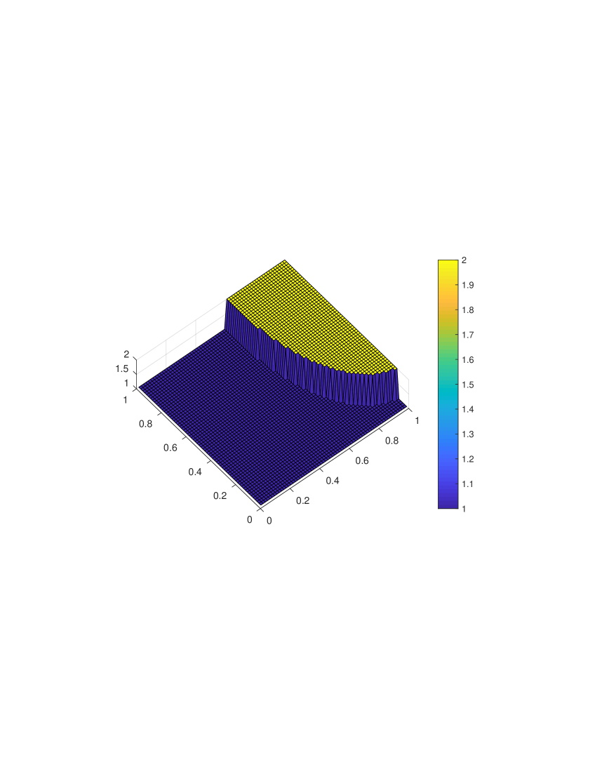
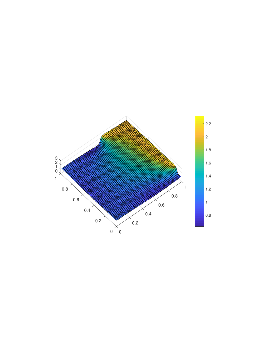
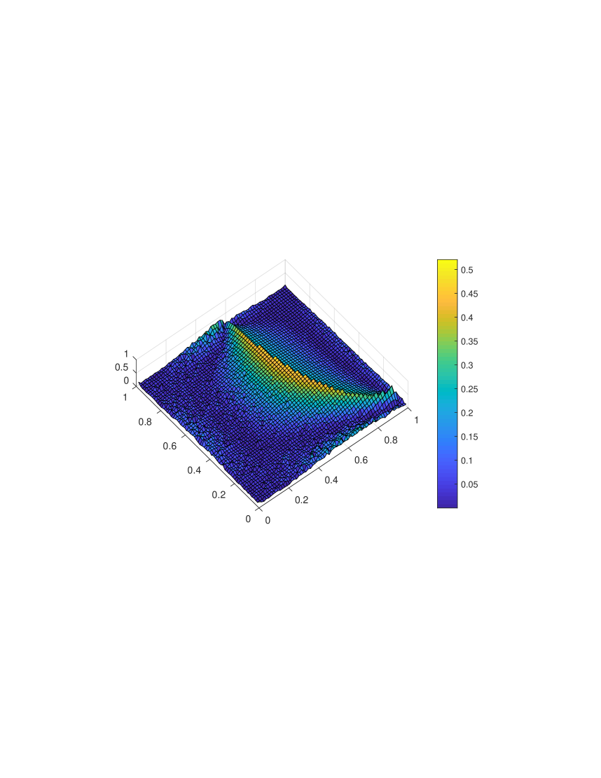
Figure 1: IPP Noise level $0.1\%$. Results obtained by the iniT method (the stopping criterion is reached at $k^{*}(\delta)=17$ steps). (TOP) Ground truth $x^{\star}$; (CENTER) Approximate solution $x_{17}^{\delta}$; (BOTTOM) Relative iteration error $|x_{17}^{\delta}-x^{\star}|/|x^{\star}|$.

The numerical experiments discussed in this section follow [11, 13]. Here, $\Omega=(0,1)\times(0,1)$ and the unknown ground truth $x^{\star}$ is assumed to be an $L_{2}$–function (see Figure 1). The iniT method is compared with the iT method. The setup of our numerical experiments is detailed as follows:

— Solve problem (32) with $x=x^{\star}$, and compute the exact data $y$.

— Add $0.1\%$ and $5\%$ of uniformly distributed random noise to the exact data, generating

the noisy data $y^{\delta}$.

— Use the constant function $x_{0}=1.5$ as initial guess for the iT and iniT methods.

— Employ the discrepancy principle with $\tau=1.5$ as the stopping criteria for the iT and

iniT methods.

— $\lambda_{k}=(\frac{2}{3})^{k}$ for both methods.

— Choose $\alpha_{k}^{\delta}$ as in Assumption 2.11 for the iniT method with

$\theta_{k}=(1/k)^{1.1}$.

— Compute $x_{k+1}^{\delta}$ in Step [2.3] of Algorithm 2; in each iteration $k=1,\dots k^{*}(\delta)$ the Conju-

gate Gradient (CG) method [20, 23], MATLAB routine with tolerance $10^{-6}$, is used to

compute the step  $s_{k}^{\delta}:=x_{k+1}^{\delta}-x_{k}^{\delta}$.

— In the iT method, obtain $x_{k+1}^{\delta}$ by solving $(\lambda_{k}A^{*}A+I)(x-x_{k}^{\delta})=\lambda_{k}A^{*}(y^{\delta}-Ax_{k}^{\delta})$ using

the MATLAB CG-routine with tolerance $10^{-6}$.

Numerical test 1 ($\mathbf{0.1\%}$ noise): The iniT method and the iT method are implemented for solving the IPP under the above described setup, reaching the stopping criteria after 17 and 19 steps respectively.

In Figure 1 the results obtained by the iniT method are presented. The stopping criterion is reached after $k^{*}(\delta)=17$ steps. The top figure shows the exact solution, the center figure displays the approximate solution $x_{17}^{\delta}$; the relative iteration error $|x_{17}^{\delta}-x^{\star}|/|x^{\star}|$ is depicted at the bottom figure. Note that the quality of the reconstruction is not as good close to the discontinuity curve of $x^{\star}$, improving farther from it.

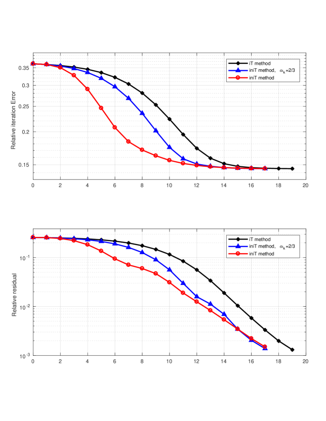
Figure 2: IPP Noise level $0.1\%$. Comparison between iT and iniT methods. (TOP) Relative iteration error; (BOTTOM) Relative residual.

The progress of the corresponding relative iteration error $\|x_{k}^{\delta}-x^{\star}\|/\|x^{\star}\|$ and relative residual $\|Ax_{k}^{\delta}-y^{\delta}\|/\|y^{\delta}\|$ are depicted in Figure 2. In each of the subplots, we display the iT method in black, and the iniT method in red. Note the presence of a third curve, in blue. That corresponds to fixing $\alpha_{k}=2/3$ constant, a choice not covered by our theory (see Numerical tests 3 below for further discussion). In Table 1 the number of CG-steps evaluated at each iteration of the methods in Figure 2 is compared.

	Iteration number
	​1	​2	​3	​4	​5	​6	​7	​8	​9	​​10	​​11	​​12	​​13	​​14	​​15	​​16	​​17	​​18	​​19
iT	​3	​3	​3	​3	​3	​4	​4	​5	​5	​​6	​​6	​​7	​​8	​​9	​​11	​​12	​​14	​​16	​​18
iniT ($\alpha_{k}=\frac{2}{3}$)	​3	​3	​3	​3	​3	​4	​4	​5	​5	​​6	​​6	​​7	​​8	​​9	​​10	​​12	​​13
iniT	​​3	​​3	​​3	​​3	​​3	​​4	​​4	​​5	​​5	​​6	​​6	​​7	​​8	​​9	​​11	​​13	​​14

Table 1: Noise level $0.1\%$. Number of CG-steps required to compute $x_{k}^{\delta}$ in each step of the methods presented in Figure 2.

The accumulated number of CG-steps of these methods read:

 

iT – 140 CG-steps   iniT ($\alpha_{k}=\frac{2}{3}$) – 104 CG-steps   iniT – 107 CG-steps

 

Notice that the iT method require $30\%$ more CG-steps than the iniT method.

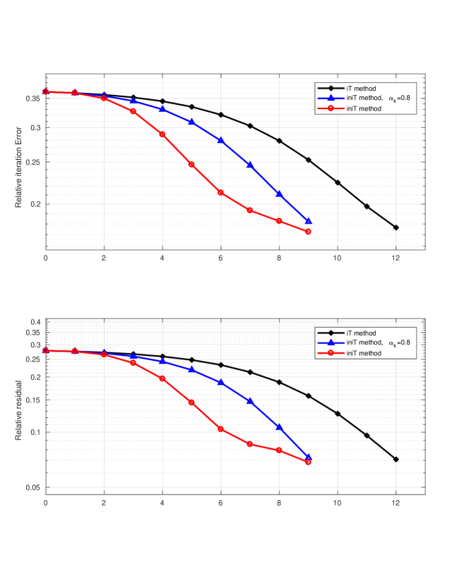
Figure 3: IPP Noise level $5.0\%$. Comparison between iT and iniT methods. (TOP) Relative iteration error; (BOTTOM) Relative residual.

Numerical test 2 ($\mathbf{5.0\%}$ noise): Similarly to the previous case, we present in Figure 3 how the iniT and iT methods perform under a $\mathbf{5.0\%}$ noise level. The stopping criteria are reached after 9 and 12 steps respectively. The subplot display the corresponding relative iteration error (top) and relative residual (bottom). The curves in black and red correspond to the iT and iniT methods. The blue curve corresponds to a constant $\alpha_{k}=2/3$ case, not covered by the theory (see Numerical tests 3 for further discussion). In Table 2 the number of CG-steps needed in each iteration of the methods presented in Figure 3 is compared.

	Iteration number
	1	2	3	4	5	6	7	8	9	10	11	12
iT	3	3	3	3	3	4	4	5	5	6	7	7
iniT ($\alpha_{k}=0.8$)	3	3	3	3	3	4	4	5	5
iniT	3	3	3	3	4	4	4	5	5

Table 2: Noise level $5.0\%$. Number of CG-steps required to compute $x_{k}^{\delta}$ in each step of the methods presented in Figure 3.

The accumulated number of CG-steps of these methods read:

 

iT – 53 CG-steps   iniT ($\alpha_{k}=0.8$) – 33 CG-steps   iniT – 34 CG-steps

 

Notice that the iT method require $56\%$ more CG-steps than the iniT method.

Numerical test 3 (experimenting with constant $\mathbf{\alpha_{k}^{\delta}}$): Observing the choice of the scaling parameters in Nesterov’s accelerated forward-backward scheme (3), a natural question arises: “How does the iniT method performs if one chooses $\alpha_{k}^{\delta}$ constant in Algorithm 2?”

Differently from the explicit two-point type methods (which include Nesterov’s scheme), in the implicit two-point methods (or inertial methods) one must assume that $\sum_{k}\alpha_{k}<\infty$ and $\sum_{k}\alpha_{k}\|x_{k}-x_{k-1}\|^{2}<\infty$. Indeed, these hypothesis are needed in the proof of the convergence Theorem 2.8 (they are used to obtain (9)). As a matter of fact, the summability of the series $\sum_{k}\alpha_{k}\|x_{k}-x_{k-1}\|^{2}$ is quintessential in our analysis: it is used to prove boundedness of the sequence $(x_{k})$ (see Proposition 2.5 (b)).

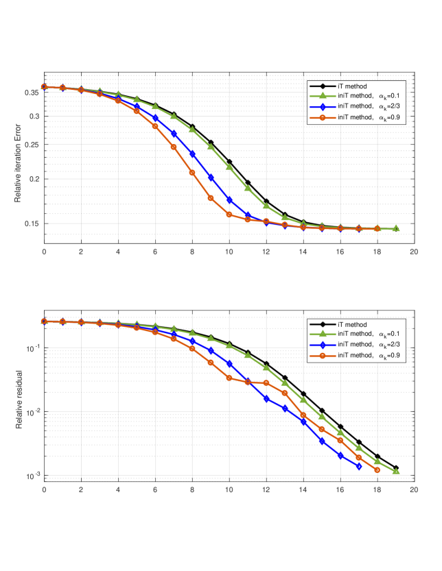
Figure 4: IPP Noise level $0.1\%$. Comparison between iT method and iniT method with constant $\alpha_{k}$. (TOP) Relative iteration error; (BOTTOM) Relative residual.

Thus, choosing $\alpha_{k}^{\delta}$ constant may not lead to bounded iterations. Nevertheless, we implemented the iniT method for different (constant) values of $\alpha_{k}^{\delta}$, ranging in the interval (0,1). In Figures 4 and 5 we revisit the noise level scenarios of $0.1\%$ and $5.0\%$ respectively.

For the noise level of $0.1\%$, the best result was obtained for $\alpha_{k}^{\delta}=2/3$, while $\alpha_{k}^{\delta}=8/10$ was the best choice for the noise level of $5.0\%$. For comparison purposes, the iniT method results with these optimal choices of (constant) $\alpha_{k}^{\delta}$ are presented in Figures 2 and 3 respectively (blue curves). Notice that:

— For (constant) $\alpha_{k}^{\delta}$ close to zero, the iniT method performs similarly as the iT method;

— For (constant) $\alpha_{k}^{\delta}$ close to one, the iniT method becomes unstable;

— The iniT method with constant choice $\alpha_{k}^{\delta}=2/3$ performs similarly as the iniT

method with $\alpha_{k}^{\delta}$ satisfying Assumption 2.11.

Numerical test 4 (comparison with explicit two-point type methods): The Nesterov’s scheme (3) and the FISTA method [7] are two well known methods for solving linear systems of the form (2). Another natural question that arises is: “How does the iniT method performance compare with performance of these established explicit two-point methods?”

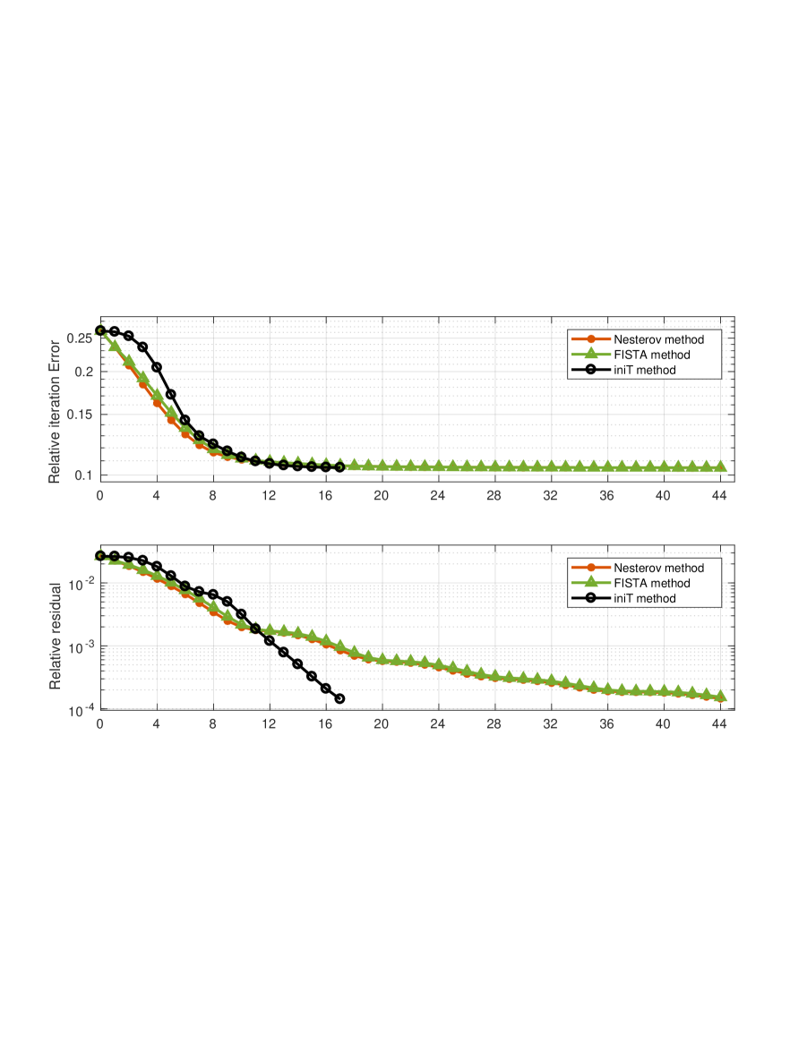
Figure 6: IPP Noise level $0.1\%$. Comparison between iniT, Nesterov and FISTA methods. (TOP) Relative iteration error; (BOTTOM) Relative residual.

To answer this question we revisit the $0.1\%$ noise scenario. In Figure 6 the iniT method (implicit), the Nesterov and the FISTA methods (both explicit) are implemented for solving the IPP. In the Nesterov and FISTA methods we use $\gamma=\|A^{*}A\|^{-1/2}$. Moreover, in the Nesterov method we set (the frequently used value) $\alpha=3.0$.

Due to the distinct nature (implicit/explicit) of these methods, the numerical effort cannot be compared by simply computing the number of iterations necessary to reach the stopping criterion. Instead, we compute the execution time of these methods:

 

iniT – 1.40 seconds   Nesterov – 6.61 seconds   FISTA – 6.76 seconds

 

3.2 The Image Deblurring Problem

The here considered Image Deblurring Problem (IDP) is an ill-posed inverse problem modeled by a finite-dimensional linear system of the form (2). In this problem $x^{\star}\in X=R^{n}$ are the pixel values of a true image, while $y\in Y=X$ represents the pixel values of the observed (blurred) image. In real situations, blurred (noisy) data $y^{\delta}\in Y$ satisfying (1) are available and the noise level $\delta>0$ is not always known.

In this setting the matrix $A$ in (2) describes the blurring process, which is modeled by a space invariant point spread function (PSF). In the continuous model, the blurring phenomena is modeled by a convolution operator and $A$ corresponds to an integral operator of the first kind [21, 17]. In our model, the discrete convolution is evaluated by means of the Fast Fourier Transform (FFT) algorithm. We added to the exact data, i.e. the true image convoluted with the PSF, a normally distributed noise with zero mean and suitable variance.

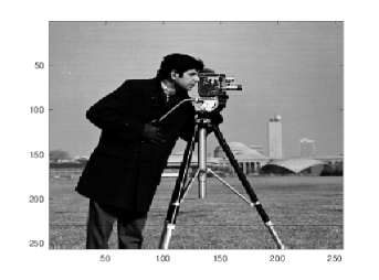
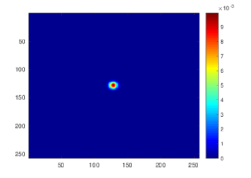
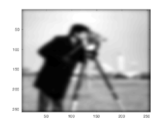
Figure 7: IDP. Setup: (LEFT) True image; (CENTER) PSF; (RIGHT) Blurred image.

In our numerical implementations we follow [11] in the experimental setup, see Figure 7: (LEFT) True image $x^{\star}\in R^{n}$, with $n=2^{16}$ (Cameraman image $256\times 256$); (CENTER) PSF is the rotationally symmetric Gaussian low-pass filter of dimension $[257\times 257]$ and standard deviation $\sigma=4$; (RIGHT) Blurred image $y=Ax\in R^{n}$.

Experiments with noisy data (IDP)

The iniT and the iT method are compared. The setup of our experiments is as follows:

— Exact data $y=Ax^{\star}=PSF*x^{\star}$ is computed.

— Noise of $0.1\%$ and $1\%$ is added to $y$, generating the noisy data $y^{\delta}$.

— The constant function $x_{0}=0$ is used as initial guess for the iT and iniT methods.

— The discrepancy principle, with $\tau=1.1$, is used as stopping criterion for all methods.

— $\lambda_{k}=(\frac{2}{3})^{k}$ in both methods.

— Choose $\alpha_{k}^{\delta}$ as in Assumption 2.11 for the iniT method with

$\theta_{k}=(1/k)^{1.1}$.

— In both iniT and iT methods the computation of $x_{k+1}^{\delta}$ is performed explicitly (in the

frequency domain the convolution corresponds to a multiplication).

Numerical test 5 (high/low noise): The iniT method and the iT method are implemented for solving the IDP under the above described setup. Two distinct levels of noise are considered, namely $\delta=0.1\%$ and $\delta=1.0\%$.

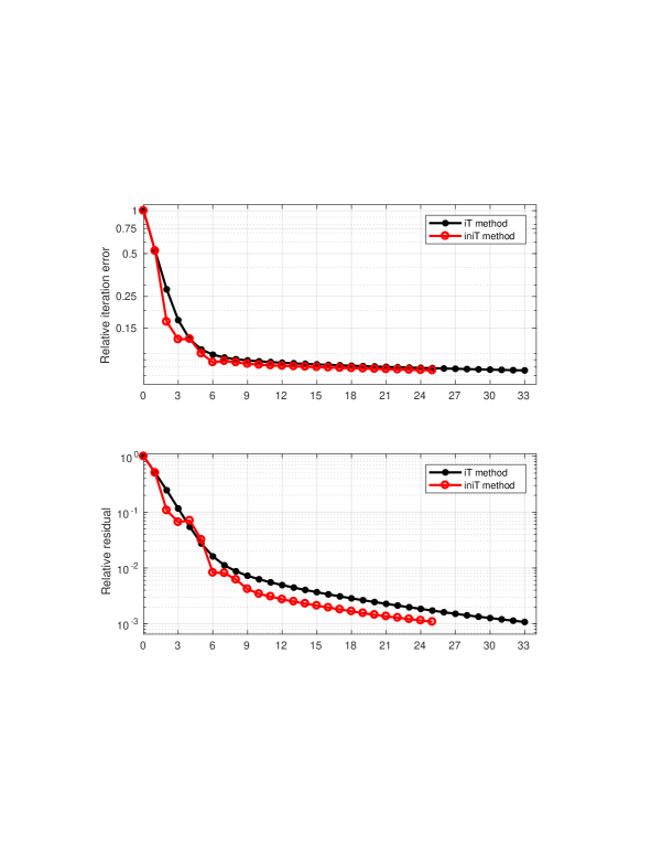
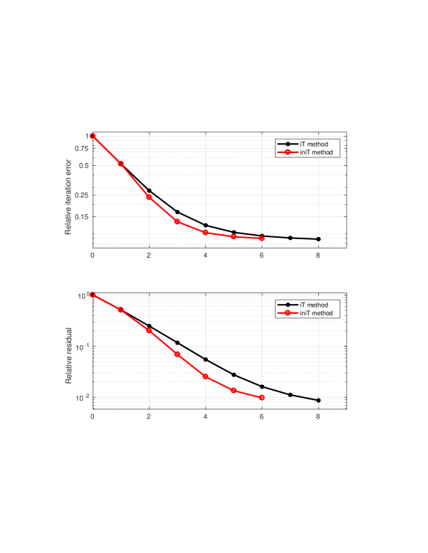
Figure 8: IDP. Relative iteration error and relative residual: (LEFT) $\delta=0.1\%$; (RIGHT) $\delta=1.0\%$.

In the $\delta=0.1\%$ noise scenario, the stopping criteria are reached after 25 and 33 steps respectively. For $\delta=1.0\%$, the stopping criteria are reached after 6 and 8 steps respectively. The progress of the corresponding relative iteration error and relative residual for both methods are presented in Figure 8. It is worth noticing that the iniT method applied to this example displays similar computational savings as discussed in Section 3.1.

4 Final remarks and conclusions

In this manuscript we propose and analyze an implicit two-point type iteration, namely the inertial iterated Tikhonov (iniT) method, as an alternative for obtaining stable approximate solutions to linear ill-posed operator equations.

The main results discussed in this notes are: boundedness of the sequences $(x_{k})$ and $(w_{k})$ generated by the iniT method (Proposition 2.5, convergence for exact data (Theorem 2.8), stability and semi-convergence for noisy data (Theorems 2.15 and 2.16 respectively).

We faced an unexpected challenge in our analysis, namely the derivation of a monotonicity result for the iteration error (i.e. $\|x_{k+1}-x^{\star}\|\leq\|x_{k}-x^{\star}\|$, where $x^{\star}$ is a solution of $Ax=y$). This is a standard result in the analysis of iterative regularization methods [17, 29], and is used to establish boundedness and convergence of $(x_{k})$. Due to the structure of the inertial iteration (5), we are only able to prove (under the current assumptions) that $\|x_{k+1}-x^{\star}\|\leq\|w_{k}-x^{\star}\|$ (see Proposition 2.5 (a)). Notice that, in order to establish the boundedness of $(x_{k})$ in Proposition 2.5 (b), we had to resort to Lemma A.1, which follows from a result by Alvarez and Attouch [2, Theorem 2.1].

The proof of the convergence result in Theorem 2.8 uses a novel strategy. The classical proof is based on a telescopic-sum argument coupled with the above mentioned monotonicity inequality. Since the monotonicity of $\|x_{k+1}-x^{\star}\|$ is not available, we used an additional assumption on $(\alpha_{k})$ (see Assumption (A2) in Theorem 2.8) in order to apply an alternative telescopic-sum argument (see (16)).

The lack of a monotonicity result also influences the verification of the stability and semi-convergence results (Theorems 2.15 and 2.16 respectively). The proofs presented here rely on properties of the sequences $(\alpha_{k}^{\delta^{j}})_{k}$ and $(\alpha_{k}^{\delta^{j}}\|x_{k}^{\delta^{j}}-x_{k-1}^{\delta^{j}}\|^{2})_{k}$.

The choice of $\theta_{k}$ in Assumptions 2.3 and 2.11 plays a key role in the numerical performance of the iniT method. In our experiments, we tried $\theta_{k}=(1/k)^{p}$ for distinct choices of $p>1$. The best results were obtained for values of $p$ close to one.

Our numerical results demonstrate that the iniT method outperforms the standard iT method (for the same choice of Lagrange multipliers $\lambda_{k}$):
$\bullet$ IPP: iniT requires $10\%$ to $20\%$ less CG-steps than iT to reach the stopping criterion.
$\bullet$ IDP: iniT requires approximately $25\%$ less iterations than iT to reach the stopping criterion.

Our numerical experiments cover two of the most relevant families of inverse problems, namely ’PDE models’ and ’integral operators models’ [5, 17, 21, 32, 42]. The benefits of the proposed iniT method, as compared to the iT method, are readily evident in all the experiments discussed. Our numerical results indicate that iniT is a competitive method for solving other highly ill-posed linear problems within these two families of problems.

Appendix A

In what follows we address a result, which is needed for the proof of Proposition 2.5. This result corresponds to a (small) part of the proof of [2, Theorem 2.1]. For the convenience of the reader, we present here a sketch of the proof.

Lemma A.1.

Let $(\alpha_{k})_{k\geq 0}\in[0,\alpha]$, with $\alpha\in(0,1)$. Moreover, let $(\varphi_{k})_{k\geq-1}$, $(\eta_{k})_{k\geq 0}$ be sequences of non-negative real numbers s.t. $\varphi_{k+1}-\varphi_{k}<\alpha_{k}(\varphi_{k}-\varphi_{k-1})+2\eta_{k}$, for $\ k\geq 0$,  and  $\sum_{k\geq 0}\eta_{k}<\infty$. There exists $\bar{\varphi}\in\mathbb{R}$ such that $\displaystyle\lim_{k\to\infty}\varphi_{k}=\bar{\varphi}$.

Proof.

Define $\gamma_{k}:=\varphi_{k}-\varphi_{k-1}$, for $k\geq 0$. Thus, it follows from the assumptions

$$\gamma_{k+1}<\alpha_{k}\gamma_{k}+2\eta_{k}\ \leq\ \alpha\gamma_{k}+2\eta_{k}\ \leq\ \alpha[\gamma_{k}]_{+}+2\eta_{k}\,,\ k\geq 0\,,$$

where $[t]_{+}:=\max\{t,0\}$, $t\in\mathbb{R}$. Consequently,  $[\gamma_{k+1}]_{+}\leq\alpha[\gamma_{k}]_{+}+2\eta_{k}\,,\ k\geq 0$. A recursive use of this inequality yields $[\gamma_{k+1}]_{+}\leq\alpha^{k+1}[\gamma_{0}]_{+}+2\sum_{j=0}^{k}\alpha^{j}\eta_{k-j}$, for $k\geq 0$. Therefore,

$$\textstyle\sum\limits_{k=0}^{\infty}[\gamma_{k+1}]_{+}\ \leq\ \displaystyle\frac{\alpha}{1-\alpha}[\gamma_{0}]_{+}\ +\ \frac{2}{1-\alpha}\textstyle\sum\limits_{k=0}^{\infty}\eta_{k}\,.$$

Since $\sum_{k\geq 0}\eta_{k}$ is summable, the right hand side is finite.

Define $\zeta_{k}:=\varphi_{k}-\sum_{j=1}^{k}[\gamma_{j}]_{+}$, for $k\geq 1$. Notice that $(\zeta_{k})$ is bounded from below. Moreover, $(\zeta_{k})$ is monotone non-increasing. Indeed,

$$\zeta_{k+1}\ =\ \varphi_{k+1}-[\gamma_{k+1}]_{+}-\textstyle\sum\limits_{j=1}^{k}[\gamma_{j}]_{+}\ \leq\ \varphi_{k+1}-(\varphi_{k+1}-\varphi_{k})-\textstyle\sum\limits_{j=1}^{k}[\gamma_{j}]_{+}\ =\ \zeta_{k}\,,\ k\geq 1\,.$$

Consequently, $(\zeta_{k})$ converges and we conclude $\lim_{k}\varphi_{k}=\sum_{j\geq 1}[\gamma_{j}]_{+}+\lim_{k}\zeta_{k}=:\bar{\varphi}$. ∎

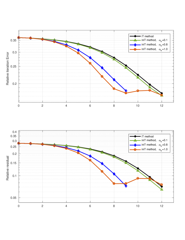
Figure 5: IPP Noise level $5.0\%$. Comparison between iT method and iniT method with constant $\alpha_{k}$. (TOP) Relative iteration error; (BOTTOM) Relative residual.

References

- [1] F. Alvarez, Weak convergence of a relaxed and inertial hybrid projection-proximal point algorithm for maximal monotone operators in Hilbert space, SIAM J. Optim. 14 (2003), no. 3, 773–782.
- [2] F. Alvarez and H. Attouch, An inertial proximal method for maximal monotone operators via discretization of a nonlinear oscillator with damping, Set-Valued Anal. 9 (2001), no. 1-2, 3–11.
- [3] R. Araya, C. Harder, D. Paredes, and F. Valentin, Multiscale hybrid-mixed method, SIAM Journal on Numerical Analysis 51 (2013), no. 6, 3505–3531.
- [4] H. Attouch and J. Peypouquet, The rate of convergence of Nesterov’s accelerated forward-backward method is actually faster than , SIAM J. Optim. 26 (2016), no. 3, 1824–1834.
- [5] J. Baumeister, Stable Solution of Inverse Problems, Advanced Lectures in Mathematics, Friedr. Vieweg & Sohn, Braunschweig, 1987. MR 889048
- [6] A. Beck, First-order methods in optimization, MOS-SIAM Series on Optimization, vol. 25, 2017.
- [7] A. Beck and M. Teboulle, A fast iterative shrinkage-thresholding algorithm for linear inverse problems, SIAM J. Imaging Sci. 2 (2009), no. 1, 183–202.
- [8] M. Bertero, Image deblurring with Poisson data: from cells to galaxies, Inverse Problems 25 (2009), no. 12, 123006.
- [9] M. Bertero and P. Boccacci, Introduction to inverse problems in imaging, Advanced Lectures in Mathematics, IOP Publishing, Bristol, 1998.
- [10] J.M. Bioucas-Dias and M.A. Figueiredo, A new TwIST: two-step iterative shrinkage/thresholding algorithms for image restoration, IEEE Trans. Image Process. 16 (2007), no. 12, 2992–3004.
- [11] R. Boiger, A. Leitão, and B.F. Svaiter, Range-relaxed criteria for choosing the Lagrange multipliers in nonstationary iterated Tikhonov method, IMA Journal of Numerical Analysis 40 (2020), no. 1, 606–627.
- [12] A. Chambolle and T. Pock, An introduction to continuous optimization for imaging, Acta Numer. 25 (2016), 161–319.
- [13] A. De Cezaro, A. Leitão, and X.-C. Tai, On multiple level-set regularization methods for inverse problems, Inverse Problems 25 (2009), 035004.
- [14] A. De Cezaro, J. Baumeister, and A. Leitão, Modified iterated Tikhonov methods for solving systems of nonlinear ill-posed equations, Inverse Probl. Imaging 5 (2011), no. 1, 1–17.
- [15] A. El Badia and M. Farah, Identification of dipole sources in an elliptic equation from boundary measurements: application to the inverse EEG problem, J. Inverse Ill-Posed Probl. 14 (2006), no. 4, 331–353.
- [16] H.W. Engl, On the choice of the regularization parameter for iterated Tikhonov regularization of ill-posed problems, J. Approx. Theory 49 (1987), no. 1, 55–63.
- [17] H.W. Engl, M. Hanke, and A. Neubauer, Regularization of Inverse Problems, Kluwer Academic Publishers, Dordrecht, 1996.
- [18] F. Frühauf, O. Scherzer, and A. Leitão, Analysis of Regularization Methods for the Solution of Ill-Posed Problems Involving Discontinuous Operators, SIAM J. Numer. Anal. 43 (2005), 767–786.
- [19] D. Gilbarg and N.S. Trudinger, Elliptic partial differential equations of second order, Grundlehren der mathematischen Wissenschaften, Springer, Berlin, 1998.
- [20] G.H. Golub and C.F. Van Loan, Matrix computations, fourth ed., Johns Hopkins Studies in the Mathematical Sciences, Johns Hopkins University Press, Baltimore, MD, 2013.
- [21] C. W. Groetsch, The Theory of Tikhonov Regularization for Fredholm Equations of the First Kind, Research Notes in Mathematics, vol. 105, Pitman (Advanced Publishing Program), Boston, MA, 1984.
- [22] C. W. Groetsch and O. Scherzer, Non-stationary iterated Tikhonov-Morozov method and third-order differential equations for the evaluation of unbounded operators, Math. Methods Appl. Sci. 23 (2000), no. 15, 1287–1300.
- [23] W. Hackbusch, Iterative Lösung großer schwachbesetzter Gleichungssysteme, Leitfäden der Angewandten Mathematik und Mechanik [Guides to Applied Mathematics and Mechanics], vol. 69, B. G. Teubner, Stuttgart, 1991, Teubner Studienbücher Mathematik. [Teubner Mathematical Textbooks].
- [24] M. Hanke and C. W. Groetsch, Nonstationary Iterated Tikhonov Regularization, J. Optim. Theory Appl. 98 (1998), no. 1, 37–53.
- [25] F. Hettlich and W. Rundell, Iterative methods for the reconstruction of an inverse potential problem, Inverse Problems 12 (1996), no. 3, 251–266.
- [26] S. Hubmer and R. Ramlau, Convergence analysis of a two-point gradient method for nonlinear ill-posed problems, Inverse Problems 33 (2017), no. 9, 095004, 30.
- [27] , Nesterov’s accelerated gradient method for nonlinear ill-posed problems with a locally convex residual functional, Inverse Problems 34 (2018), no. 9, 095003, 30.
- [28] Victor Isakov, Inverse Problems for Partial Differential Equations, second ed., Applied Mathematical Sciences, vol. 127, Springer, New York, 2006.
- [29] B. Kaltenbacher, A. Neubauer, and O. Scherzer, Iterative Regularization Methods for Nonlinear Ill-Posed Problems, Radon Series on Computational and Applied Mathematics, vol. 6, Walter de Gruyter GmbH & Co. KG, Berlin, 2008.
- [30] S. Kindermann, Optimal-order convergence of Nesterov acceleration for linear ill-posed problems, Inverse Problems 37 (2021), no. 6, Paper No. 065002, 21.
- [31] S. Kindermann and A. Neubauer, On the convergence of the quasioptimality criterion for (iterated) Tikhonov regularization, Inverse Probl. Imaging 2 (2008), no. 2, 291–299.
- [32] A. Kirsch, An Introduction to the Mathematical Theory of Inverse Problems, Applied Mathematical Sciences, vol. 120, Springer-Verlag, New York, 1996.
- [33] L. Landweber, An iteration formula for Fredholm integral equations of the first kind, Amer. J. Math. 73 (1951), 615–624.
- [34] A. Leitão and B.F. Svaiter, On a family of gradient type projection methods for nonlinear ill-posed problems, Numerical Functional Analysis and Optimization 39 (2018), no. 11, 1153–1180.
- [35] A.L. Madureira and M. Sarkis, Hybrid Localized Spectral Decomposition for Multiscale Problems, SIAM J. Numer. Anal. 59 (2021), no. 2, 829–863.
- [36] B. Martinet, Régularisation d’inéquations variationnelles par approximations successives, Rev. Française Informat. Recherche Opérationnelle 4 (1970), no. Sér. R-3, 154–158.
- [37] A. Moudafi and M. Oliny, Convergence of a splitting inertial proximal method for monotone operators, J. Comput. Appl. Math. 155 (2003), no. 2, 447–454.
- [38] Y.E. Nesterov, A method for solving the convex programming problem with convergence rate , Dokl. Akad. Nauk SSSR 269 (1983), no. 3, 543–547.
- [39] A. Neubauer, On Nesterov acceleration for Landweber iteration of linear ill-posed problems, J. Inverse Ill-Posed Probl. 25 (2017), no. 3, 381–390.
- [40] P. Ochs, Y. Chen, T. Brox, and T. Pock, iPiano: inertial proximal algorithm for nonconvex optimization, SIAM J. Imaging Sci. 7 (2014), no. 2, 1388–1419.
- [41] P.A. Raviart and J.M. Thomas, Primal Hybrid Finite Element Methods for 2nd Order Elliptic Equations, Mathematics of Computation 31 (1977), no. 138, 391+.
- [42] A. Rieder, Keine Probleme mit inversen Problemen, Friedr. Vieweg & Sohn, Braunschweig, 2003, Eine Einführung in ihre stabile Lösung. [An introduction to their stable solution].
- [43] R.T. Rockafellar, Monotone operators and the proximal point algorithm, SIAM J. Control Optim. 14 (1976), no. 5, 877–898.
- [44] O. Scherzer, Convergence rates of iterated Tikhonov regularized solutions of nonlinear ill-posed problems, Numer. Math. 66 (1993), no. 2, 259–279.
- [45] , A convergence analysis of a method of steepest descent and a two-step algorithm for nonlinear ill-posed problems, Numer. Funct. Anal. Optim. 17 (1996), no. 1-2, 197–214.
- [46] K. van den Doel, U. M. Ascher, and A. Leitão, Multiple Level Sets for Piecewise Constant Surface Reconstruction in Highly Ill-Posed Problems, Journal of Scientific Computing 43 (2010), no. 1, 44–66.
- [47] Kees van den Doel, Uri M. Ascher, and Dinesh K. Pai, Computed myography: three-dimensional reconstruction of motor functions from surface EMG data, Inverse Problems 24 (2008), no. 6, 065010, 17.