Regularized Q-Learning with Linear Function Approximation

Abstract

Several successful reinforcement learning algorithms make use of regularization to promote multi-modal policies that exhibit enhanced exploration and robustness. With functional approximation, the convergence properties of some of these algorithms (e.g. soft Q-learning) are not well understood. In this paper, we consider a single-loop algorithm for minimizing the projected Bellman error with finite time convergence guarantees in the case of linear function approximation. The algorithm operates on two scales: a slower scale for updating the target network of the state-action values, and a faster scale for approximating the Bellman backups in the subspace of the span of basis vectors. We show that, under certain assumptions, the proposed algorithm converges to a stationary point in the presence of Markovian noise. In addition, we provide a performance guarantee for the policies derived from the proposed algorithm.

Linear function approximation, Q-learning, reinforcement learning.

1 Introduction

Numerous reinforcement learning algorithms have achieved remarkable success by employing some form of regularization [1, 2]. The specific choice of regularization choices induces a specific trade-off between exploration and exploitation. For example, negative Shannon entropy regularization has been successfully employed in [3, 2]. In that case, the learned policies are robust to perturbations in both the dynamics and the reward function [4]. Regularization can also be used to impose sparsity of learned policies (e.g., Tsallis entropy [5, 6, 7]). This approach maintains a multi-modal policy form but restricts the support to only optimal and near-optimal actions, thereby mitigating the impact of detrimental actions. Recent studies [8, 7] develop the framework for analyzing regularized Markov Decision Processes (MDPs) with a broad class of regularizers. The regularized MDPs are proven to exhibit robustness in scenarios where the reward function is uncertain [9], and they boast a faster convergence rate during policy optimization [10, 11, 12, 13]. In this study, we investigate the convergence properties of an off-policy algorithm tailored for approximating the optimal value function in MDPs equipped with strongly convex regularizers, within the context of linear function approximation.

Q-learning, as presented in [14], is a model-free, off-policy reinforcement learning algorithm. While it has demonstrated convergence in tabular settings [15], its convergence performance degrades with larger discount factors. Recently, a novel variant termed ‘relative Q-learning’ was introduced in [16]; it is designed to provide uniform bounds on sample complexity, regardless of the discount factor. However, the convergence of Q-learning with linear function approximation has not been formally established except under restrictive assumptions, such as an exceedingly small discount factor [17, 18]. Generally, the function obtained by applying the Bellman operator to a function within the span of predefined features cannot be expressed as a linear combination of these features [19]. The Bellman operator exhibits contraction properties with respect to the $\ell_{\infty}$-norm, and the projection onto the span of predefined features is non-expansive with respect to the $\ell_{2}$-norm. However, when these operators are composed to form the projected Bellman operator, the resulting operator does not necessarily retain the contraction property with respect to any norm. As a consequence, divergence may occur during the iteration process [20]. A substantial body of work has been devoted to developing variants of the Q-learning algorithm to overcome this issue. [21, 22] demonstrate convergence by employing ridge regularization on the approximator (also referred to as the main network); however, these approaches solve an MDP with a decreased discount factor instead of the original problem. [23] demonstrated asymptotic convergence, and further extended the framework to a linear function approximation scheme subject to specific conditions on the features. Introducing a target network, which is a delayed copy of the main network, has been shown to effectively stabilize the off-policy learning process in deep reinforcement learning [24]. Within Coupled Q-learning [25], the target network undergoes updates at a slower rate instead of copying the main network. Although the convergence of the aforementioned methods is established, the quality of the convergent points is ensured only with a sufficiently low discount factor. Zap Zero algorithm [26] approximates the Newton-Raphon flow without matrix inversion and is guaranteed to converge to the optimal solution under mild assumptions. Greedy Gradient Q-learning (Greedy-GQ) with linear function approximation is a provably convergent algorithm under mild assumptions [27]. The algorithm utilizes gradient descent and seeks to minimize the Mean-Square Projected Bellman Error (MSPBE), which is non-convex in general. The finite-time convergence guarantees to the stationary points were established recently in [28, 29, 30, 31]. Recent work [32] demonstrates that employing a target network, in conjunction with the truncation operator on Bellman backup values, effectively confines the estimated value function within a desirable neighbor of the optimal value function.

1.1 Our Contributions

We have developed an algorithm with finite-time guarantees for learning the solution to a broad class of regularized Markov Decision Processes (MDPs) using linear function approximation. Our contributions are as follows:

• We introduce a smooth truncation operator that is applied to the Bellman backup in regularized MDPs, preserving the smoothness of the regularized Bellman operator.

• We propose a bi-level formulation for regularized Q-learning with target (upper level) and main (lower level) solution (or network), respectively. In this approach, the lower-level problem is to find the projected Bellman backup for the target network – this is a strongly convex problem. The upper-level problem aims to determine the optimal target network parameter $\theta^{*}$ that minimizes the non-convex Mean-Square Projected Bellman Error (MSPBE), denoted as $J(\theta)$, which incorporates a smooth truncation operator. This formulation serves as a foundation for the development of the proposed algorithm.

• We develop a single-loop algorithm to learn the solution of the proposed bi-level formulation in the presence of Markovian noise. Notably, we demonstrate that the algorithm converges to a stationary point at a rate $T^{-1}\sum_{t=0}^{T-1}\mathbb{E}\|\nabla J(\theta^{t})\|=\mathcal{O}(T^{-1/4})$. Moreover, we establish finite-time performance guarantees for the learned policies. These guarantees reveal that, compared to the optimal policy, the expected performance gap of policies obtained in $T>0$ iterations is $\mathcal{O}(T^{-1/4})$, augmented by the function approximation error and the error introduced by the smooth truncation operator.

• We carry out numerical experiments to illustrate the impact of errors introduced by the smooth truncation operator on the solution quality. Additionally, our evaluation of policies derived from the proposed algorithms reveals superior performance compared to existing methods in most scenarios.

1.2 Related Work

A large number of studies have been done on variants of the Q-learning algorithm within the framework of function approximation. In this subsection, we briefly discuss some works that are most closely related to our work.

The stability of Q-learning and its related variants, particularly in the context of function approximation, has long been a focus of research [33, 34]. Numerous techniques have been proposed to address these stability concerns, including the target network [24], double estimator [35], fitted value iteration [36], gradient-based approaches [27], and stochastic Newton-Raphson [37], among others. Furthermore, ensuring the convergence of these variant algorithms remains a more significant challenge in the field of reinforcement learning, even when employing linear function approximation [32, 33].

Zap Q-learning [38, 37] and its variant, Zap Zero [26], mimic the classical Newton-Raphson algorithm. These algorithms guarantee asymptotic convergence under mild assumptions, though they come with substantial computational costs due to matrix inversion or its approximation process.

Greedy-GQ [27], inspired by the success of TDC in off-policy evaluation [19], employs a two-timescale gradient-based approach to minimize the MSPBE, and its asymptotic convergence to a stationary point is established over i.i.d. sampled data. Recent work [30] provides a finite-time guarantee for the convergence of Greedy-GQ under Markovian noise with a rate of $\mathcal{O}(T^{-1/3}\log T)$, and it has been improved to $\mathcal{O}(T^{-1/2}\log T)$ in [29], albeit without providing guarantees for the boundedness of the iterates. Subsequent work [31] further improves the result to $\mathcal{O}(T^{-1/2})$ with the use of a mini-batch gradient. It should be noted that the criteria they employ, in terms of rate, diverge from ours, given their consideration of the square of the gradient’s norm. While our approach bears similarities to Greedy-GQ in its formulation, the objectives differ. Greedy-GQ’s lower-level problem seeks to approximate the TD error, whereas our method focuses on maintaining a main network to approximate Bellman backups within the span of the basis. Moreover, we utilize the truncation and projection operators to ensure the boundedness of the iterates without compromising the convergence rate.

Employing ridge regularization in Q-learning allows for convergence guarantees with linear function approximation, without imposing stringent assumptions [21, 22]. However, this approach diverges from addressing the original problem, as it inherently reduces the discount factor. In contrast, our work views the regularized MDP as the original problem in which it is the policy, not the value function, that is regularized. Our proposed updates the main network in the same manner as in Coupled Q-learning [25], while the target network in Coupled Q-learning is updated toward the fixed point of the composed operator constructed by combining the ”un-normalized” orthogonal projection and the Bellman operator. Consequently, unlike our algorithm which focuses on minimizing a specific objective function, Coupled Q-Learning does not target the minimization of any particular objective. While Coupled Q-learning converges asymptotically without stringent assumptions, its estimated value function proves meaningful only with a low discount factor.

Over-parameterized neural networks serve as non-linear function approximators and have found extensive applications in various reinforcement learning algorithms. These include TD-learning [39], the policy gradient method [40], and Q-learning [41, 42]. Furthermore, recent studies have established finite-sample bounds for these algorithms [43, 44, 45]. However, over-parameterization typically necessitates a neural network with a sufficiently large width, a scenario in which the functions in the considered function class are nearly linear around the initialization point [46]. In contrast, the linear function approximation employed in this study generally operates under the ‘under-parameterized’ framework, which can not only lower computational costs in practice but also yield deeper insights into under-parameterized cases. More importantly, neural network-based estimations are less interpretable compared to those using linear function approximation. In the latter case, feature selection is usually driven by an understanding of the model and specific interests.

2 Preliminaries

In this section, we present the preliminaries for regularized Q-learning. We denote the dot product as $\langle\cdot,\cdot\rangle$. The $\ell_{2}$ and $\ell_{\infty}$ norms are denoted by $\|\cdot\|$ and $\|\cdot\|_{\infty}$, respectively.

2.1 Regularized Markov Decision Process

We consider an infinite-horizon regularized Markov Decision Processes (MDPs) with finite action space. An MDP can be described as a tuple $\mathcal{M}\triangleq\left(\mathcal{S},\mathcal{A},P,\mu_{0},R,\gamma\right)$, where $\mathcal{S}$ denotes the state space and $\mathcal{A}$ denotes the action space. $P$ is the dynamics: $P(s^{\prime}\mid s,a)$ is the transition probability from state $s$ to $s^{\prime}$ by taking action $a$. $\mu_{0}$ is the initial distribution of the state. The reward function, $R:\mathcal{S}\times\mathcal{A}\rightarrow\mathbb{R}$, is bounded in absolute value by $R_{\max}\geq 0$ for all $(s,a)\in\mathcal{S}\times\mathcal{A}$. $\gamma\in(0,1)$ is the discount factor. A policy $\pi:\mathcal{S}\rightarrow\Delta(\mathcal{A})$ is defined as a mapping from the state space $\mathcal{S}$ to the probability distribution over the action space $\mathcal{A}$. For discrete time $t\geq 0$, the trajectory, starting from an initial state $s_{0}\sim\mu_{0}(\cdot)$, generated by the policy $\pi$ in the MDP $\mathcal{M}$ can be represented as a set of transition tuples $\left\{s_{t},a_{t},s_{t}^{\prime}\right\}_{t\geq 0}$, where $a_{t}\sim\pi(\cdot\mid s_{t})$, $s_{t}^{\prime}\sim P(\cdot\mid s_{t},a_{t})$, and $s_{t+1}=s_{t}^{\prime},\forall t\geq 0$.

Let $G:\Delta(\mathcal{A})\rightarrow\mathbb{R}$ be a strongly convex bounded function, where there exists a constant $B>0$ such that $|G(p)|\leq B$ for all $p\in\Delta(\mathcal{A})$. Then the convex conjugate of $G^{*}:\mathbb{R}^{|\mathcal{A}|}\rightarrow\mathbb{R}$ is given by

$$G^{*}(q)=\max_{p\in\Delta(\mathcal{A})}\left\langle p,q\right\rangle-G(p),\quad\forall q\in\mathbb{R}^{|\mathcal{A}|}.$$

One commonly used choice of $G$ is negative Shannon entropy; in that case $G(p)=\left\langle p,\log p\right\rangle$, and the convex conjugate is $G^{*}(q)=\log\left(\left\langle\exp(q),\boldsymbol{1}\right\rangle\right)$, where $\boldsymbol{1}$ is the vector of ones. Another example is a specific form of negative Tsallis entropy, $G(p)=\frac{1}{2}(\left\|p\right\|^{2}-1)$, which leads to a sparse MDP [5]. For the sake of clarity, we define $G_{\tau}\triangleq\tau\cdot G$, where $\tau>0$ is a positive coefficient that determines the degree of regularization applied. Consequently, the convex conjugate of $G_{\tau}$ is

$$G_{\tau}^{*}(q)=\max_{p\in\Delta(\mathcal{A})}\left\langle p,q\right\rangle-G_{\tau}(p)=\tau\cdot G^{*}(q/\tau),\quad\forall q\in\mathbb{R}^{|\mathcal{A}|}.$$

Unlike the unregularized MDP, the objective of a regularized MDP $\mathcal{M}_{\tau}$ is to maximize not only the expected cumulative reward but also include a policy regularization term [7]. The regularized state-action value function under a given policy $\pi$, starting from a specific state-action pair $(s,a)$, is defined as

$$Q_{\pi,\tau}(s,a)=R(s,a)\\ +\mathbb{E}\bigg{[}\sum_{t=1}^{\infty}\gamma^{t}\big{(}R\left(s_{t},a_{t}\right)-G_{\tau}(\pi(\cdot\mid s_{t}))\big{)}\bigg{|}s_{0}=s,a_{0}=a,P,\pi\bigg{]}.$$

In a similar manner, the regularized state value function can be defined as

$$V_{\pi,\tau}(s)= \mathbb{E}\left[\sum_{t=0}^{\infty}\gamma^{t}\left(R\left(s_{t},a_{t}\right)-G_{\tau}(\pi(\cdot\mid s_{t}))\right)\bigg{|}s_{0}=s,P,\pi\right]$$

$$= \mathbb{E}_{a\sim\pi(\cdot\mid s)}\left[Q_{\pi,\tau}(s,a)\right]-G_{\tau}\left(\pi\left(\cdot\mid s\right)\right);$$ (1)

this quantity represents the expected cumulative sum of rewards and regularization terms, commencing from state $s$ and adhering to policy $\pi$ subsequently, within the MDP $\mathcal{M}_{\tau}$ governed by dynamics $P$.

Some properties of regularized MDPs are stated in the following proposition. For a detailed analysis, see [8].

Proposition 2.1

Let $G$ be a strongly convex function bounded by $B>0$ and $\tau>0$ be a coefficient associated with $G$. The following hold:

1. The gradient of the convex conjugate with respect to the input $q$ is $\nabla G_{\tau}^{*}(q)=\arg\max_{p\in\Delta(\mathcal{A})}\left\langle p,q\right\rangle-G_{\tau}(p),\forall q\in\mathbb{R}^{|\mathcal{A}|}$. $\nabla G_{\tau}^{*}$ is $\frac{L_{G}}{\tau}$-Lipschitz, i.e., there exists a constant $L_{G}>0$ such that $\left\|\nabla G_{\tau}^{*}(q_{1})-\nabla G_{\tau}^{*}(q_{2})\right\|\leq\frac{L_{G}}{\tau}\left\|q_{1}-q_{2}\right\|,\forall q_{1},q_{2}\in\mathbb{R}^{|\mathcal{A}|}$.

2. The conjugate function is bounded: $|G^{*}_{\tau}\left(q\right)-\max_{i}q_{(i)}|\leq\tau B,\forall q\in\mathbb{R}^{|\mathcal{A}|}$, where $q_{(i)}$ is the $i$-th element of the vector $q$.

3. For any policy $\pi$, the regularized value functions $V_{\pi,\tau}$ and $Q_{\pi,\tau}$ satisfy regularized Bellman equation, for all $(s,a)\in\mathcal{S}\times\mathcal{A}$:

   $$Q_{\pi,\tau}(s,a)=R(s,a)+\gamma\mathbb{E}_{s^{\prime}\sim P\left(\cdot\mid s,a\right)}\left[V_{\pi,\tau}\left(s^{\prime}\right)\right].$$

4. The optimal state value function $V^{*}_{\tau}(s)=\max_{\pi}V_{\pi,\tau}(s)=G^{*}_{\tau}\left(Q^{*}_{\tau}\left(s,\cdot\right)\right),\forall s\in\mathcal{S}$, where $Q^{*}_{\tau}(\cdot,\cdot)$ is the optimal state-action value function and, for all $(s,a)\in\mathcal{S}\times\mathcal{A}$, it satisfies

   $$Q^{*}_{\tau}(s,a)= R(s,a)+\gamma\mathbb{E}_{s^{\prime}\sim P\left(\cdot\mid s,a\right)}\left[V^{*}_{\tau}\left(s^{\prime}\right)\right].$$

   This equation is commonly referred to as the optimal regularized Bellman equation.

5. The optimal policy $\pi^{*}_{\tau}(\cdot\mid s)=\nabla G^{*}_{\tau}\left(Q^{*}_{\tau}\left(s,\cdot\right)\right)$, for all $s\in\mathcal{S}$.

Given properties in Proposition 2.1, we define the regularized Bellman operator $\mathcal{B}_{\tau}$ as, for an arbitrary mapping $X:\mathcal{S}\times\mathcal{A}\rightarrow\mathbb{R}$:

$$\mathcal{B}_{\tau}X(s,a)\triangleq R(s,a)+\gamma\mathbb{E}_{s^{\prime}\sim P(\cdot\mid s,a)}\left[G^{*}_{\tau}\left(X\left(s^{\prime},\cdot\right)\right)\right],$$

and it is $\gamma$-contraction in $\ell_{\infty}$-norm [8]. Observe that the optimal state-action value function $Q^{*}_{\tau}$ is the unique fixed point of the optimal regularized Bellman operator: $Q^{*}_{\tau}=\mathcal{B}_{\tau}Q^{*}_{\tau}$. This fixed point can be derived through value iteration.

2.2 Linear Function Approximation

In environments with large state spaces, such as continuous spaces, maintaining a lookup table to store and process values for all possible state-action pairs is impractical. Function approximation techniques are prevalent as they offer an effective solution to this problem by allowing agents to approximate the values using significantly fewer parameters. In this study, we focus on leveraging linear function approximation which approximates the value functions linearly in the given basis vectors. The basis vectors $\phi_{i}\in\mathbb{R}^{|\mathcal{S}||\mathcal{A}|}$, $i=1,2,\dots,d$ are, without loss of generality, linearly independent. We denote $\phi(s,a)=\left[\phi_{1}(s,a),\phi_{2}(s,a),\dots,\phi_{d}(s,a)\right]^{\top}\in\mathbb{R}^{d}$ for all $(s,a)$ and let $\Phi\in\mathbb{R}^{|\mathcal{S}||\mathcal{A}|\times d}$ defined by $\Phi=\left[\phi(s_{1},a_{1}),\dots,\phi(s_{|\mathcal{S}|},a_{|\mathcal{A}|})\right]^{\top}$. We approximate state-action function as $\hat{Q}_{\theta}\triangleq\Phi\theta$, where $\theta\in\mathbb{R}^{d}$ is the parameter vector. We also use $\hat{Q}_{\theta}(s,\cdot)=\phi(s,\cdot)^{\top}\theta$ to denote the vector of the approximated state-action values of all actions given the state $s\in\mathcal{S}$, where $\phi(s,\cdot)=\left[\phi(s,a_{1}),\dots,\phi(s,a_{|\mathcal{A}|})\right]$. Suppose $\mu$ is a distribution that exhibits full support across the state-action space, let $D_{\mu}\in\mathbb{R}^{|\mathcal{S}||\mathcal{A}|\times|\mathcal{S}||\mathcal{A}|}$ be a diagonal matrix with the distribution $\mu$ on its diagonal. Furthermore, we define the weighted $\ell_{2}$-norm with respect to the distribution $\mu$ as $\|x\|_{D_{\mu}}\triangleq\sqrt{x^{\top}D_{\mu}x}$. Let $\Pi_{D_{\mu}}$ be the projection operator which maps a vector onto the span of the basis functions with respect to the norm $\|\cdot\|_{D_{\mu}}$; it is given by $\Pi_{D_{\mu}}=\Phi\left(\Phi^{\top}D_{\mu}\Phi\right)^{-1}\Phi^{\top}D_{\mu}$ under the assumption that $\Phi^{\top}D_{\mu}\Phi$ is a positive definite matrix.

Within the framework of linear function approximation, the primary objective of value function estimation is to determine an optimal parameter $\theta^{*}$ that satisfies the regularized projected Bellman equation: $\hat{Q}_{\theta^{*}}=\Pi_{D_{\mu}}\mathcal{B}_{\tau}\hat{Q}_{\theta^{*}}$, where $\mu$ is given. While the projection operator $\Pi_{D_{\mu}}$ is known to be a weighted $\ell_{2}$ non-expansive mapping, it is important to note that the composite operator $\Pi_{D_{\mu}}\mathcal{B}_{\tau}$ does not generally exhibit contraction properties with respect to any norm [32].

3 Problem Formulation

3.1 Smooth Truncation Operator

Motivated by the stabilization of using the truncation operator within linear function approximation as highlighted in [32], we explore a smooth variant of this operator. This adaptation maintains the smoothness of Bellman backups in regularized MDPs and is particularly advantageous for gradient-based algorithms, which are our primary focus. For a threshold $\delta>0$, we define the smooth truncation operator $\mathcal{K}$ as

$$\mathcal{K}_{\delta}(x)\triangleq\delta\cdot\tanh\left(\frac{x}{\delta}\right),\quad\forall x\in\mathbb{R},$$

where $\tanh$ is the hyperbolic tangent function; the particular choice of the operator is not essential – alternative choices are feasible. Consequently, $\mathcal{K}_{\delta}$ maps any value in $\mathbb{R}$ to the interval $(-\delta,\delta)$. We define $\hat{G}_{\tau,\delta}$ as the composite operator formed by applying the smooth truncation operator $\mathcal{K}_{\delta}$ to the convex conjugate $G_{\tau}^{*}$ of the regularizer, i.e.

$$\hat{G}_{\tau,\delta}(q)=\mathcal{K}_{\delta}\left(G_{\tau}^{*}\left(q\right)\right),\forall q\in\mathbb{R}^{|\mathcal{A}|}.$$

In addition, we let $\mathcal{B}_{\tau,\delta}$ be the smooth truncated optimal regularized Bellman operator which is given as, for an arbitrary mapping $X:\mathcal{S}\times\mathcal{A}\rightarrow\mathbb{R}$:

$$\mathcal{B}_{\tau,\delta}X(s,a)\triangleq R(s,a)+\gamma\mathbb{E}_{s^{\prime}\sim P(\cdot\mid s,a)}\left[\hat{G}_{\tau,\delta}\left(X\left(s^{\prime},\cdot\right)\right)\right],$$

which preserves the property of $\gamma$-contraction in $\ell_{\infty}$-norm.

In contrast to the hard truncation operator $\lceil x\rceil_{\delta}\triangleq\max\{\min\{x,\delta\},-\delta\}$, $\mathcal{K}_{\delta}$ is differentiable everywhere on $\mathbb{R}$, with the gradient given by

$$\nabla\mathcal{K}_{\delta}(x)=1-\tanh^{2}\left(\frac{x}{\delta}\right)=1-\frac{\mathcal{K}^{2}_{\delta}(x)}{\delta^{2}},$$

which equals $1$ at $x=0$ and approaches $0$ as $|x|\to\infty$. It is evident that $|\mathcal{K}_{\delta}(x)|\leq|\lceil x\rceil_{\delta}|\leq|x|$ for all $x\in\mathbb{R}$. This property can be beneficial in mitigating the overestimation issue. However, there is a trade-off involving the gap between $\mathcal{K}_{\delta}(x)$ and $x$ when $x$ is away from the origin. On the other hand, as the value of $|\frac{x}{\delta}|$ decreases, $\mathcal{K}_{\delta}(x)$ approaches closer to $x$. Therefore, we have the inequality

$$\left|x-\mathcal{K}_{\delta}(x)\right|\leq\left|y-\mathcal{K}_{\delta}(y)\right|\text{ if }|x|\leq|y|\in\mathbb{R}.$$ (2)

Further investigation of the threshold $\delta$ is presented in Section 6.

3.2 Bi-level Formulation

Before presenting the problem formulation, we outline some assumptions that are crucial for our analysis. Let $\pi_{\mathrm{bhv}}$ be the behavioral policy used to collect data in regularized MDP $\mathcal{M}_{\tau}$ and we adopt the following assumption.

Assumption 3.1

The behavioral policy $\pi_{\mathrm{bhv}}$ satisfies $\pi_{\mathrm{bhv}}(a\mid s)>0$ for all $(s,a)$, and the Markov chain induced by it is irreducible and aperiodic. Then there exist constants $\kappa>0$ and $\rho\in(0,1)$ such that

$$\sup_{s_{0}\in\mathcal{S}}d_{TV}\left(\mathbb{P}\left(\left(s_{t},a_{t}\right)\in\cdot\mid s_{0},\pi_{\mathrm{bhv}},P\right),\mu_{\mathrm{bhv}}\right)\leq\kappa\rho^{t},\quad\forall t,$$

where $d_{TV}$ is the total-variation distance and $\mu_{\mathrm{bhv}}$ is the stationary distribution of state-action pairs.

Assumption 3.1 guarantees the ergodicity of the Markov chain, which in turn ensures that it converges to its stationary distribution at a geometric rate. Furthermore, Let $\mathcal{D}$ be the stationary distribution of the transition tuples induced by $\pi_{\mathrm{bhv}}$. Consequently, $\mathcal{D}=\mu_{\mathrm{bhv}}\otimes P$, where $\otimes$ denotes the tensor product between two distributions. We use the term $\mathcal{D}$ to also refer to the marginal distribution of state-action pairs, i.e., $\mathcal{D}(s,a)=\mu_{\mathrm{bhv}}(s,a)$ for all $(s,a)\in\mathcal{S}\times\mathcal{A}$, with a slight abuse of notation.

Additionally, the following standard (e.g., see [47, 48, 30]) assumption is adopted in our work. It can be ensured by normalizing the features.

Assumption 3.2

$\left\|\phi(s,a)\right\|_{2}\leq 1,\forall(s,a)\in\mathcal{S}\times\mathcal{A}$.

In this study, our primary focus is the estimation of state-action value functions, which we achieve by minimizing the Mean Squared Projected Bellman Error (MSPBE) through the application of smooth truncation operator:

$$J(\theta)=\frac{1}{2}\mathbb{E}_{\mathcal{D}}\left(\Pi\mathcal{B}_{\tau,\delta}\hat{Q}_{\theta}(s,a)-\hat{Q}_{\theta}(s,a)\right)^{2}.$$

Calculating the projected Bellman backup $\Pi\mathcal{B}_{\tau,\delta}\hat{Q}_{\theta}(s,a)$ presents significant challenges. This has motivated the development of the bi-level optimization formulation detailed below:

$$\quad\min_{\theta\in\mathbb{R}^{d}}J\left(\theta\right) \triangleq f\left(\theta,\omega^{*}(\theta)\right)$$ (3)

$$\triangleq\frac{1}{2}\mathbb{E}_{\mathcal{D}}\left(\phi(s,a)^{\top}\omega^{*}\left(\theta\right)-\phi(s,a)^{\top}\theta\right)^{2}$$

$$\textit{s.t.}\quad\omega^{*}\left(\theta\right) \in\arg\min_{\omega\in\mathbb{R}^{d}}g(\theta,\omega),$$

where the lower-level objective is

$$g(\theta,\omega)\triangleq\frac{1}{2}\mathbb{E}_{\mathcal{D}}\left(\phi(s,a)^{\top}\omega-R(s,a)-\gamma\hat{G}_{\tau,\delta}(\hat{Q}_{\theta}\left(s^{\prime},\cdot\right))\right)^{2}.$$

In this context, $\omega$ represents the parameters of the main network, and $\theta$ represents the parameters of the target network.

In prior successful algorithms [49, 24, 50], the target network serves as a delayed replica of the main network, stabilizing the learning process and reducing overestimation. To achieve this, the target network’s parameters are updated less frequently or using smaller step sizes compared to the main network, enabling the target network to offer a slower-moving target for state-action value function estimates. The goal of updating the target deviates from simply mimicking the main network. Instead, the target network is updated with the objective of minimizing the MSPBE with smooth truncation. A key distinction in our application of the smooth truncation operator, compared to the approach in [32], lies in its implementation. We apply it to the state value function, whereas [32] employs it on the state-action value function. As a result, the policies corresponding to $Q\in\mathbb{R}^{|\mathcal{S}||\mathcal{A}|}$ remain unchanged in the regularized MDP. We define the regularized policy $\pi_{\theta}$ corresponding to the approximated regularized state-action value function $\hat{Q}_{\theta}$ as

$$\pi_{\theta}(\cdot\mid s)\triangleq\nabla G^{*}_{\tau}\left(\hat{Q}_{\theta}\left(s,\cdot\right)\right),\quad\forall s\in\mathcal{S}.$$ (4)

The strong convexity of $g(\theta,\omega)$ in $\omega$ is established in the following proposition, which can be proved by using Taylor’s expansion.

Proposition 3.3

Under Assumption 3.1, there exists a constant $\lambda_{g}>0$ that lower bounds the eigenvalue of $\Sigma\triangleq\mathbb{E}_{\mathcal{D}}[\phi(s,a)\phi(s,a)^{\top}]$. Consequently, $g(\theta,\omega)$ is strongly convex in $\omega$ for any $\theta\in\mathbb{R}^{d}$, and with modulus $\lambda_{g}/2$. That is, for any $\omega_{1},\omega_{2}\in\mathbb{R}^{d}$, $\theta\in\mathbb{R}^{d}$,

$$g(\theta,\omega_{1})\geq g(\theta,\omega_{2})+\left\langle\nabla_{\omega}g(\theta,\omega_{2}),\omega_{1}-\omega_{2}\right\rangle+\frac{\lambda_{g}}{2}\|\omega_{1}-\omega_{2}\|^{2}.$$

The lower-level problem’s objective function aims to identify $\omega^{*}(\theta)$, an optimal weight of the approximation of the Bellman backup for a target network parameterized by $\theta$, within the subspace spanned by the basis functions. It is given by

$$\!\!\!\omega^{*}(\theta)=\Sigma^{-1}\mathbb{E}_{\mathcal{D}}\!\left[\phi(s,a)\left(\!R(s,a)+\gamma\hat{G}_{\tau,\delta}(\hat{Q}_{\theta}\left(s^{\prime},\cdot\right))\right)\right].$$ (5)

Under Assumption 3.1 and 3.2, the $\ell_{2}$-norm of $\omega^{*}(\theta)$ is bounded by $(R_{\max}+\gamma\delta)/\lambda_{g}$. In this case, the optimal value, $g(\theta,\omega^{*}(\theta))$, from the lower-level problem characterizes the square of the approximation error with respect to $\hat{Q}_{\theta}$ under the distribution $\mathcal{D}$. This error represents the component of $\mathcal{B}_{\tau,\delta}\hat{Q}_{\theta}$ that is not captured within the span of the basis functions. $\hat{Q}_{\omega^{*}(\theta)}=\Phi\omega^{*}(\theta)$ represents the projection of $\mathcal{B}_{\tau,\delta}\hat{Q}_{\theta}$ onto the space spanned by the basis functions with respect to the norm $\|\cdot\|_{D_{\mu_{\mathrm{bhv}}}}$, i.e. $\hat{Q}_{\omega^{*}(\theta)}=\Pi_{D_{\mu_{\mathrm{bhv}}}}\mathcal{B}_{\tau,\delta}\hat{Q}_{\theta}$. To simplify the presentation, we adopt a shorthand notation by using $\Pi$ to represent $\Pi_{D_{\mu_{\mathrm{bhv}}}}$ throughout the rest of this paper, albeit with a slight abuse of notation.

The optimization problem (3) can be solved by a gradient-based approach. The gradient of $J(\theta)$ can be derived by using the chain rule as

$$\nabla J(\theta)$$

$$= \nabla_{\theta}f(\theta,\omega^{*}(\theta))$$

$$-\nabla^{2}_{\theta\omega}g(\theta,\omega^{*}(\theta))\left[\nabla^{2}_{\omega\omega}g(\theta,\omega^{*}(\theta))\right]^{-1}\nabla_{\omega}f(\theta,\omega^{*}(\theta))$$

$$= \hat{\Sigma}_{\tau,\delta,\theta}\left(\omega^{*}(\theta)-\theta\right),$$ (6)

where

$$\hat{\Sigma}_{\tau,\delta,\theta}\triangleq$$

$$\mathbb{E}_{\mathcal{D}}\!\!\left[\!\left(\!\!\gamma z\left(s^{\prime};\tau,\delta,\theta\right)\!\sum_{a^{\prime}\in\mathcal{A}}\!\!\!\pi_{\theta}\left(a^{\prime}\mid s^{\prime}\right)\phi\left(s^{\prime},a^{\prime}\right)-\phi(s,a)\!\!\right)\!\phi(s,a)^{\top}\!\right],$$ (7)

and

$$z\left(s;\tau,\delta,\theta\right)\triangleq 1-\frac{1}{\delta^{2}}\hat{G}^{2}_{\tau,\delta}(\hat{Q}_{\theta}(s,\cdot)),\quad\forall s\in\mathcal{S}.$$ (8)

Observe that the range of $z$ is $(0,1)$. The following assumption is important in our analysis.

Assumption 3.4

For $\theta\in\mathbb{R}^{d}$, the matrix $\hat{\Sigma}_{\tau,\delta,\theta}$ is non-singular. Therefore, there exists a constant $\sigma_{\min}>0$ that lower bounds the smallest singular value of it for all $\theta\in\mathbb{R}^{d}$.

As the threshold $\delta$ approaches infinity, the smooth truncation operator $\mathcal{K}_{\delta}$ becomes equivalent to the identity function. Under these conditions, it is clear that $z\left(s;\tau,\delta,\theta\right)$ approaches $1$ for every $s\in\mathcal{S}$ given a finite value of $\theta$. Consequently, Assumption 3.4 is as strong as similar assumptions in [27, 51, 37, 23, 18, 52, 31]. Nonetheless, when $\delta$ has a finite value, Assumption 3.4 is weaker, especially for a small value of $\delta$.

It is computationally expensive to calculate $\nabla J(\theta)$ during implementation. Alternatively, we can employ a two-timescale algorithm to simultaneously update the parameters $\theta$ and $\omega$, each operating on a different timescale. For the upper-level problem, the surrogate gradient $\bar{\nabla}_{\theta}f(\theta,\omega)$ is used with $\omega^{*}(\theta)$ replaced by $\omega$ in (3.2), defining the surrogate gradient as

$$\bar{\nabla}_{\theta}f(\theta,\omega)=\hat{\Sigma}_{\tau,\delta,\theta}\left(\omega-\theta\right).$$ (9)

In addition, the surrogate gradient can be readily sampled under a stochastic setting, similar to the gradient of the lower-level objective function, which is given by

$$\nabla_{\omega}g(\theta,\omega)=\\ \mathbb{E}_{\mathcal{D}}\Big{[}\phi(s,a)\Big{(}\phi(s,a)^{\top}\omega-R(s,a)-\gamma\hat{G}_{\tau,\delta}(\hat{Q}_{\theta}\left(s^{\prime},\cdot\right))\Big{)}\Big{]}.$$

One of the approaches for solving bi-level optimization problems is two-timescale algorithm. It simultaneously updates both the lower-level and upper-level solutions, with convergence guaranteed by employing a faster timescale for the lower-level solution and a slower timescale for the upper-level solution [53, 54, 55]. Within this framework, the target network, $\hat{Q}_{\theta}$, is updated at a slower pace compared to the main network, $\hat{Q}_{\omega}$, in our problem.

4 The Proposed Algorithm

Algorithm 1 Single-loop Regularized Q-learning

1:  Input: Constant $T$, step sizes $\alpha,\beta$, initial parameters $\omega^{0},\theta^{0}$, behavioral policy $\pi_{\mathrm{bhv}}$.

2:  Sample Initial State: $s_{0}\sim\mu_{0}(\cdot)$.

3:  for $t=0,\dots,T-1$ do

4:     Sample Action and Subsequent State:

4:       $a_{t}\sim\pi_{\mathrm{bhv}}(\cdot\mid s_{t}),s_{t}^{\prime}\sim P(\cdot\mid s_{t},a_{t})$.

5:     Estimate Lower-Level Gradient:

5:       compute $h_{g}^{t}$ by performing (10a).

6:     Update Lower-Level Parameter: perform (11a).

7:     Estimate Upper-Level Gradient:

7:       compute $h_{f}^{t}$ by performing (10b).

8:     Update Upper-Level Parameter: perform (11b).

9:     Update State: $s_{t+1}=s_{t}^{\prime}$.

10:  end for

In this section, we introduce a gradient-based single-loop algorithm that extends the two-timescale stochastic approximation (TTSA) approach, as outlined in [55]. Our focus is on estimating the value functions of the regularized MDP with linear function approximation. We explore this problem within a framework characterized by Markovian noise, noting that our results can also be extended to settings with i.i.d. noise. We use $(s_{t},a_{t},s_{t}^{\prime})$ to represent the $t$-th transition on the Markov chain induced by $\pi_{\mathrm{bhv}}$ on MDP $\mathcal{M}_{\tau}$. The action $a_{t}$ is sampled from $\pi_{\mathrm{bhv}}(\cdot\mid s_{t})$ and the next state $s_{t+1}=s_{t}^{\prime}$, which is drawn from $P(\cdot\mid s_{t},a_{t})$. The stochastic gradient of the lower-level problem and the stochastic surrogate gradient of the upper-level problem are represented by

$$h_{g}^{t}\triangleq\phi(s_{t},a_{t})\left(\phi(s_{t},a_{t})^{\top}\omega^{t}-R(s_{t},a_{t})-\gamma\hat{G}_{\tau,\delta}(\hat{Q}_{\theta^{t}}\left(s^{\prime}_{t},\cdot\right))\right)$$ (10a)

and

$$h_{f}^{t}\triangleq\bigg{(}\gamma z\left(s^{\prime};\tau,\delta,\theta\right)\sum_{a^{\prime}\in\mathcal{A}} \pi_{\theta^{t}}\left(a^{\prime}\mid s^{\prime}_{t}\right)\phi(s_{t}^{\prime},a^{\prime})-\phi(s_{t},a_{t})\bigg{)}$$

$$\times\phi(s_{t},a_{t})^{\top}\left(\omega^{t+1}-\theta^{t}\right),$$ (10b)

respectively. Recall the definition of $\pi_{\theta}$ in (4), which represents the optimal policy derived from the state-action value estimation of the target network, $\hat{Q}_{\theta}$. The parameters are updated with the step sizes $\alpha$ and $\beta$ in the following sense:

$$\omega^{t+1} =\mathcal{P}\left(\omega^{t}-\beta h_{g}^{t}\right),$$ (11a)

$$\theta^{t+1} =\begin{cases}\theta^{t}-\frac{\alpha}{\|\theta^{t}-\omega^{t+1}\|}h_{f}^{t}\quad&\text{if }\theta^{t}\neq\omega^{t+1},\\ \theta^{t}\quad&\text{otherwise,}\end{cases}$$ (11b)

where $\mathcal{P}$ denotes the projection onto $\ell_{2}$-balls with a radius of $(R_{\max}+\gamma\delta)/\lambda_{g}$. This value ensures that the optimal point $\omega^{*}(\theta^{t})$ of the lower-level problem lies within the specified ball. Utilizing the projection $\mathcal{P}$ constrains the main network, preventing it from taking overly large steps in the incorrect direction [48, 56, 52].

The update rule for the upper-level problem in Algorithm 1 sets it apart from existing two-timescale algorithms for off-policy value function estimation [27, 25, 28, 52, 31]. Specifically, it normalizes the stochastic gradient by dividing it by the difference between the weights of the main and target networks. Further analysis is provided in Section 5. See the two-timescale regularized Q-learning with adaptive stepsize in Algorithm 1.

5 Finite-Time Guarantees

In this section, we present the finite-time convergence guarantee for Algorithm 1 and the performance bound of the derived policies.

5.1 Convergence Analysis

Many current gradient-based algorithms depend on the objective function’s smooth property, a characteristic not present in problem (3). We address this by considering a relaxed version of smoothness.

Lemma 5.1

(Relaxation of smoothness.) Suppose Assumptions 3.1, 3.2 hold, for all $\theta_{1},\theta_{2}\in\mathbb{R}^{d}$, then

$$\left\|\nabla J\left(\theta_{1}\right)-\nabla J\left(\theta_{2}\right)\right\|\leq\left(L_{0}+L_{1}\left\|\omega^{*}\left(\theta_{2}\right)-\theta_{2}\right\|\right)\left\|\theta_{1}-\theta_{2}\right\|,$$

where $L_{0}=4/\lambda_{g}$ and $L_{1}=L_{G}|\mathcal{A}|/\tau+2/\delta$. Moreover, the following holds:

$$J\left(\theta_{1}\right)-J\left(\theta_{2}\right) -\left\langle\nabla J\left(\theta_{2}\right),\theta_{1}-\theta_{2}\right\rangle$$

$$\ \ \ \leq\frac{L_{0}+L_{1}\left\|\omega^{*}\left(\theta_{2}\right)-\theta_{2}\right\|}{2}\left\|\theta_{1}-\theta_{2}\right\|^{2}.$$

We refer the readers to Appendix 10.1 for detailed proof. A similar property termed $(L_{0},L_{1})$-smoothness is incorporated into the optimization algorithm, enhancing the speed of resolution, as demonstrated in [57, 58]. By employing the smooth truncation operator to impose bounds and integrating the projection operation as illustrated in equation (11a), we ensure that the $\ell_{2}$-norm of the stochastic gradient of the lower-level problem is constrained.

Lemma 5.2

Under Assumption 3.2, we have

$$\left\|h_{g}^{t}\right\|\leq\frac{2\left(R_{\max}+\delta\right)}{\lambda_{g}},\ \text{for }t=0,1,\dots,T-1.$$

The detailed proof can be found in Appendix 10.2.

We present the finite-time convergence guarantees of Algorithm 1 in the following theorem.

Theorem 5.3

Suppose Assumptions 3.1, 3.2 and 3.4 hold. Let $\alpha=\alpha_{0}T^{-3/4},\beta=\beta_{0}T^{-1/2}$ and $\alpha<\frac{\sigma_{\min}^{2}}{2(L_{1}+\sigma_{\min})}$, where $\alpha_{0},\beta_{0}$ are positive constants. Then, Algorithm 1 yields

$$\frac{1}{T}\sum_{t=0}^{T-1}\mathbb{E}\left\|\omega^{*}(\theta^{t})-\omega^{t+1}\right\|=\mathcal{O}\left(T^{-1/4}\right)$$ (12a)

and

$$\frac{1}{T}\sum_{t=0}^{T-1}\mathbb{E}\left\|\bar{\nabla}f\left(\theta^{t},\omega^{t+1}\right)\right\|=\mathcal{O}\left(T^{-1/4}\right).$$ (12b)

Consequently, the average $\ell_{2}$-norm of the gradient of the objective function satisfies

$$\frac{1}{T}\sum_{t=0}^{T-1}\mathbb{E}\left\|\nabla J\left(\theta^{t}\right)\right\|=\mathcal{O}\left(T^{-1/4}\right).$$ (13)

The detailed proof can be found in Appendix 9.1.

Observe that the bounds outlined in Theorem 5.3 are expressed in terms of $\ell_{2}$ norms. This is different from the conventional use of squared $\ell_{2}$ norms prevalent in the majority of two-timescale convergent algorithms, as demonstrated in [55, 52, 31, 28, 59, 29, 30]. The primary reason for this distinction lies in the normalization of the gradient employed in update (11b), which is common in the optimization techniques like normalized or clipped gradient-based algorithms. However, it can be inferred that the norm scaling at an order of $T^{-1/4}$ is roughly equivalent to the squared norm scaling at an order of $T^{-1/2}$, albeit with a slight discrepancy.

Remark 5.4

The rates in (12a) and (13) have components that are inversely proportional to the square of $\lambda_{g}$, the lower bound of the eigenvalue of $\Sigma$. This suggests that a larger $\lambda_{g}$ leads to faster convergence of the lower-level problem, thereby enhancing the convergence of the upper-level problem. Additionally, a high value of $\lambda_{g}$, along with a large coefficient $\tau$, augments the smoothness of the objective function, as established in Lemma 5.1. Furthermore, the rates in (12b) and (13) include components inversely proportional to $\sigma_{\min}$, the lower bound of the singular value of the matrix $\Sigma_{\tau,\delta,\theta}$. Increased smoothness in $J$, together with a large $\sigma_{\min}$, allows for a greater step size $\alpha$. This, in practice, accelerates convergence. The effect of the threshold $\delta$ on the rates in Theorem 5.3 is more complex, and we defer the discussion to Section 6.

Remark 5.5

The convergence rate of Algorithm 1 is constrained by the convergence rate (12a) of its lower-level problem. In a nested loop algorithm framework, where the lower-level problem is optimally solved in each iteration, we have $\omega^{t+1}=\omega^{*}(\theta^{t})$ and $\bar{\nabla}f(\theta^{t},\omega^{t+1})=\nabla J(\theta^{t})$. As a result, the bound defined in $\eqref{eq: J_grad}$ can be achieved as $\mathcal{O}(T^{-1/2})$ by choosing a step size $\alpha=\alpha_{0}T^{-1/2}$, where $T$ denotes the total number of iterations for updating the target network $\hat{Q}_{\theta^{t}}$.

We also demonstrate that the target network converges to the main network.

Corollary 5.6

The target network $\hat{Q}_{\theta^{t}}$ converges to the main network $\hat{Q}_{\omega^{t}}$ at a rate given by

$$\frac{1}{T}\sum_{t=0}^{T-1}\mathbb{E}\left\|\theta^{t}-\omega^{t}\right\|=\mathcal{O}\left(T^{-1/4}\right).$$

The detailed proof is in Appendix 11.1.

5.2 Performance Analysis

In this subsection, we analyze the difference between the estimated state-action value function $\hat{Q}_{\theta}$ and the optimal value function $Q^{*}_{\tau}$ in $\mathcal{M}_{\tau}$. Additionally, we compare the performance of policies derived from Algorithm 1 against the optimal policies $\pi^{*}_{\tau}$.

The approximation error in our linear function approximation setting is defined as

$$\mathcal{E}_{\mathrm{approx}}\triangleq\sup_{\theta\in\mathbb{R}^{d}}\left\|\Pi\mathcal{B}_{\tau,\delta}\hat{Q}_{\theta}-\mathcal{B}_{\tau,\delta}\hat{Q}_{\theta}\right\|_{\infty}.$$ (14)

This error quantifies the representational power of the linear approximation architecture [47]. With additional information about the problems we are targeting, the space containing $\theta$ to be considered can be narrowed. Consequently, this leads to a further reduction in the approximation error. Also, we define

$$\delta_{0}\triangleq\frac{R_{\max}+\tau B}{1-\gamma},$$

which serves as an upper bound for all state value functions in $\mathcal{M}_{\tau}$.

The performance of a policy $\pi$ is measured by $\mathbb{E}_{s\sim\mu_{0}}\left[V_{\pi,\tau}(s)\right]$ in regularized MDP $\mathcal{M}_{\tau}$, recall the definition of $V_{\pi,\tau}$ in (2.1). This expression quantifies the expected cumulative rewards and regularization terms starting from the initial state. Consequently, $\mathbb{E}_{s\sim\mu_{0}}\left[V_{\tau}^{*}(s)-V_{\pi_{\theta^{t}},\tau}(s)\right]$ captures the expected improvement achievable when transitioning from policy $\pi_{\theta^{t}}$ to the optimal policy $\pi_{\tau}^{*}$. To quantify this disparity in performance, we employ the $\ell_{\infty}$-norm which offers uniform upper bounds on the expected improvements. In the following theorem, we present the finite-time bound characterizing the difference between the estimated value function and the optimal value functions, and the performance guarantee for the sequence of policies $\left\{\pi_{\theta^{t}}\right\}_{t=0}^{T-1}$ produced by Algorithm 1.

Theorem 5.7

Suppose Assumptions 3.1, 3.2 and 3.4 hold. Then Algorithm 1 yields

$$\frac{1-\gamma}{T} \sum_{t=0}^{T-1}\mathbb{E}\left\|Q^{*}_{\tau}-\hat{Q}_{\theta^{t}}\right\|_{\infty}$$

$$\leq \frac{1}{\sigma_{\min}T}\sum_{t=0}^{T-1}\mathbb{E}\left\|\nabla J\left(\theta^{t}\right)\right\|+\mathcal{E}_{\mathrm{approx}}+\gamma\left(\delta_{0}-\mathcal{K}_{\delta}\left(\delta_{0}\right)\right),$$ (15)

and

$$\frac{1-\gamma}{2T} \sum_{t=0}^{T-1}\mathbb{E}\left\|V_{\tau}^{*}-V_{\pi_{\theta^{t}},\tau}\right\|_{\infty}$$

$$\leq \frac{1}{\sigma_{\min}T}\sum_{t=0}^{T-1}\mathbb{E}\left\|\nabla J\left(\theta^{t}\right)\right\|+\mathcal{E}_{\mathrm{approx}}+\gamma\left(\delta_{0}-\mathcal{K}_{\delta}\left(\delta_{0}\right)\right),$$ (16)

The detailed proof can be found in Appendix 9.2.

The first term in (5.7) can be bounded by leveraging Theorem 5.3. The term $\mathcal{E}_{\mathrm{approx}}$ is generally non-removable, a characteristic echoed in much of the literature on RL with linear function approximation [60, 25, 32]. The last term arises from the application of the smooth truncation operator $\mathcal{K}_{\delta}$. We defer the discussion of this term to Section 6.

The second bound in Theorem 5.7 establishes, to the best of our knowledge, the first performance guarantee of the derived policies for a convergent algorithm that learns the solution of the regularized MDP with linear function approximation. As the approximation error nears zero and the effect of the smooth truncation diminishes, the learned policy $\pi_{\theta^{t}}$ converges towards the optimal policy $\pi^{*}_{\tau}$. This convergence is realized under the condition of Bellman Completeness [61], provided that the threshold $\delta$ is also sufficiently large.

6 A Discussion on Threshold $\delta$

The threshold $\delta$ utilized in [32] is set at $R_{\max}/(1-\gamma)$ for the hard truncation operator. This value ensures that the true optimal value function $Q^{*}$ is not excluded from the candidate function space under the Bellman completeness condition.

In our context, consider a function class

$$\mathcal{Q}_{\delta}\triangleq\{\Phi\theta:\|\Phi\theta\|_{D_{\mu_{\mathrm{bhv}}}}\leq R_{\max}+\gamma\delta,\theta\in\mathbb{R}^{d}\}.$$

We can ensure that $Q_{\tau}^{*}\in\mathcal{Q}_{\delta}$, provided that $Q_{\tau}^{*}$ is within the subspace of the linear span of the basis functions $\{\phi_{i}\}_{i=1}^{d}$, by choosing $\delta\geq\delta_{0}$.

We assert that the projected smooth truncated optimal regularized Bellman backup of a state-action value function $\hat{Q}$, expressed as $\Pi\mathcal{B}_{\tau,\delta}\hat{Q}$, is also an element of $\mathcal{Q}_{\delta}$ for each $\hat{Q}\in\mathcal{Q}_{\delta}$, i.e., $\Pi\mathcal{B}_{\tau,\delta}\hat{Q}\in\mathcal{Q}_{\delta},\forall\hat{Q}\in\mathcal{Q}_{\delta}$. Given that $\mathcal{Q}_{\delta}$ is both convex and compact, the Brouwer fixed-point theorem ensures the existence of at least one fixed point $\hat{Q}^{*}\in\mathcal{Q}_{\delta}$ such that $\hat{Q}^{*}=\Pi\mathcal{B}_{\tau,\delta}\hat{Q}^{*}$. It is noteworthy that this assurance is absent when dealing with the composed operator $\Pi\mathcal{B}_{\tau}$ where truncation is not present.

Unfortunately, $Q_{\tau}^{*}$ is not a fixed point of $\Pi\mathcal{B}_{\tau,\delta}$ even when $Q_{\tau}^{*}\in\mathcal{Q}_{\delta}$, except for the case where $V_{\tau}^{*}=\boldsymbol{0}$. Recall that the error induced by the smooth truncation operator is also accounted for in the bounds specified in Theorems 5.7. To address this challenge, choosing a larger value of $\delta$ is beneficial due to the following inequality:

$$\left|x-\mathcal{K}_{\delta_{1}}\left(x\right)\right|\leq\left|x-\mathcal{K}_{\delta_{2}}\left(x\right)\right|,\ \forall x\in\mathbb{R},\delta_{1}\geq\delta_{2}\in\mathbb{R}.$$ (17)

This suggests that by opting for a sufficiently large $\delta$, the operator $\mathcal{B}_{\tau,\delta}$ can be made to closely approximate $\mathcal{B}_{\tau}$, reducing the bias in Theorem 5.7. For instance, opting for $\delta=\delta_{0}$ gives us the gap $\delta_{0}-\mathcal{K}_{\delta}\left(\delta_{0}\right)\approx 0.2384\delta_{0}$. By selecting a threshold of $\delta=10\delta_{0}$, we can significantly reduce this error, as demonstrated by $\delta_{0}-\mathcal{K}_{\delta}\left(\delta_{0}\right)\approx 0.0033\delta_{0}$.

The drawbacks of a large threshold value for $\delta$ are two-fold. Firstly, a larger value of $\delta$ increases the $\ell_{2}$-norms of both the stochastic gradient $h_{g}^{t}$ and the optimal point $\omega^{*}(\theta^{t})$ in the lower-level problem. This leads to a higher variance in both the main network and the target network, affecting the convergence bounds as outlined in Theorem 5.3. More specifically, the bound in (12a) increases linearly, and the bound in (12b) increases quadratically with $\delta$ when $\delta$ is large. Secondly, an increase in $\delta$ correlates with potential higher approximation error, as defined in (14). This escalation adversely affects the accuracy of the estimated value functions, potentially undermining the performance of the resulting policies in the worst case.

A smaller $\delta$, similar to the effect of the coefficient $\tau$, reduces the smoothness of the function $J$, as detailed in Lemma 1. More importantly, the application of the smooth truncation operator $\mathcal{K}\delta$ subtly alters the discount factor $\gamma$. This modification is different from the methods used in [21, 22], which uniformly reduce the discount factor across all states. In contrast, the use of $\mathcal{K}_{\delta}$ results in a more significant impact on states $s$ with values $|G^{*}_{\tau}(\hat{Q}_{\theta}(s,\cdot))|$ close to $\delta$, for which $z(s;\tau,\delta,\theta)$ is small, while states with values closed to $0$ are affected to a lesser extent. However, a small $\delta$ affects more states than a large $\delta$ and consequently introduces a larger bias in the bounds stated in Theorem 5.7, as it effectively transforms the problem into one with a significantly smaller discount factor.

7 Numerical Illustration

In this section, we explore two environments: GridWorld and MountainCar-v0. We begin with the GridWorld environment, where we elucidate the influences of the smooth truncation operator $\mathcal{K}_{\delta}$ on the fixed points. Graphical illustrations complement our discussion, offering a visual representation of the convergence of the estimation from the proposed algorithm and illustrating the reduction in MSPBE. Subsequently, we assess the policies derived from our algorithm within the MountainCar-v0 environment and compare their performance with policies stemming from existing algorithms.

7.1 GridWorld

We investigate the influence of the smooth truncation operator within a discrete GridWorld setting, characterized by a $5\times 5$ state space and five possible actions: up, down, left, right, and stay. We consider the context of an entropy-regularized Markov Decision Process (MDP), employing a regularizer $G(\pi(\cdot\mid s))=\langle\pi(\cdot\mid s),\log\pi(\cdot\mid s)\rangle$ with a coefficient $\tau=1$, and a discount factor $\gamma=0.9$. The dynamics of agent movement are straightforward. The agent transitions between states as directed by its chosen action, except when attempting to cross the grid boundaries, where it remains at its current state. The initial distribution is set to be uniform across all states, a setup that extends to the behavior policy as the probability of each possible action is the same. Consequently, each state-action pair in the space $\mathcal{S}\times\mathcal{A}$ has an equal likelihood of occurrence, leading to a stationary distribution $\mu_{\mathrm{bhv}}(s,a)=\frac{1}{|\mathcal{S}|\times|\mathcal{A}|}=\frac{1}{125}$ for all $(s,a)$. The reward for each state is depicted in Fig. 1(a).

We adopt second-order polynomial functions of the state as basis functions. Fig. 1(b) depicts the optimal regularized value function $V_{\tau}$. We conduct a comparison of the fixed point and the projected regularized Bellman equation, exploring scenarios both with and without the incorporation of a smooth truncation operator, all within the context of linear function approximation. The threshold of the smooth truncation $\mathcal{K}_{\delta}$ is defined as $\delta=c\delta_{0}=\frac{c(1+\log 5)}{1-\gamma}$, with $c$ taking values of $1$, $10$, and $30$.

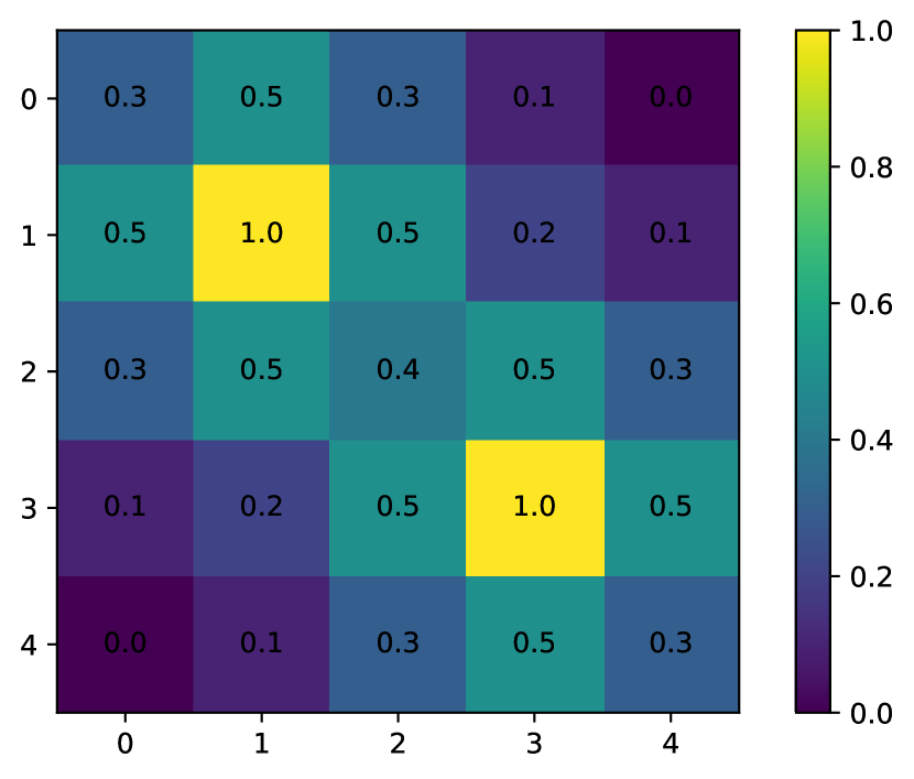
(a) Rewards Map $R$.

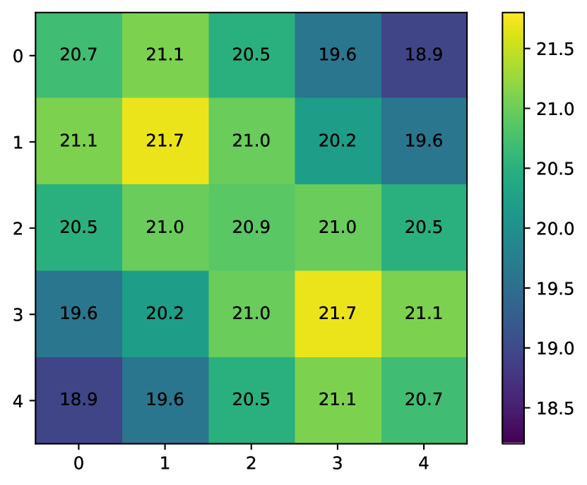
(b) True Value Map $V^{*}_{\tau}$.

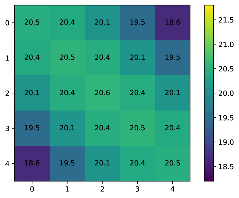
(c) Fixed Point of $\Pi\mathcal{B}_{\tau}$

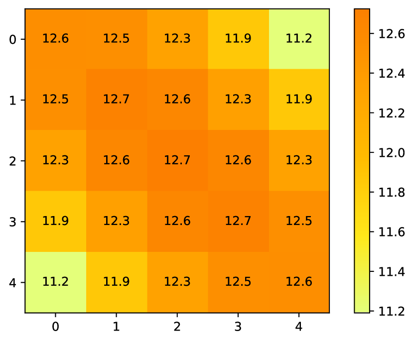
(d) Fixed Point of $\Pi\mathcal{B}_{\tau,\delta_{0}}$

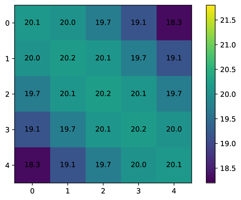
(e) Fixed Point of $\Pi\mathcal{B}_{\tau,10\delta_{0}}$

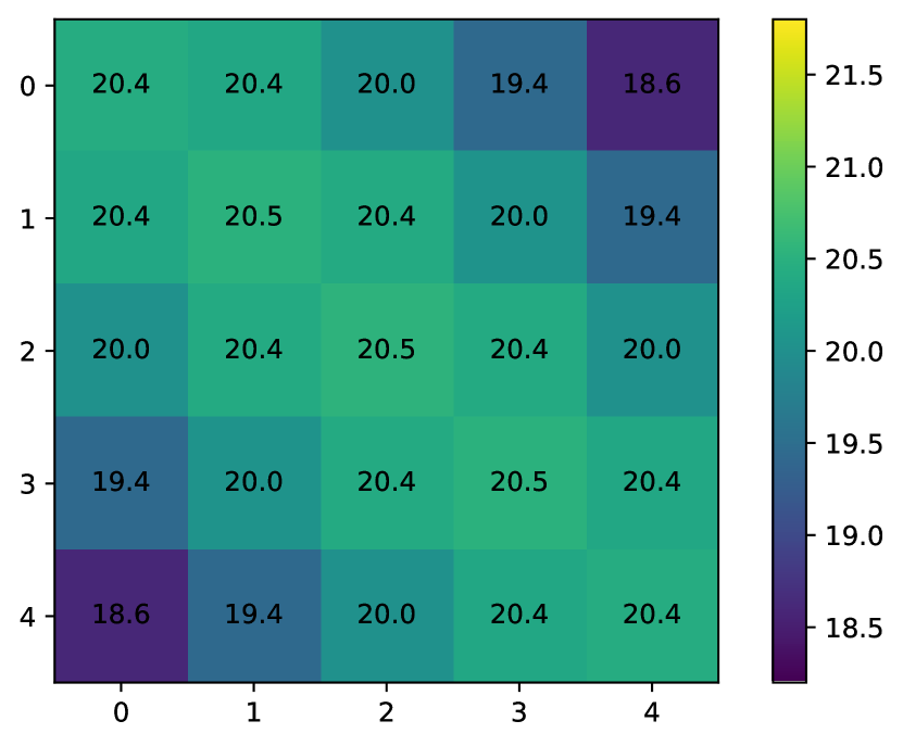
(f) Fixed Point of $\Pi\mathcal{B}_{\tau,30\delta_{0}}$

Figure 1: Rewards and Values Maps.

From the plots, it is evident that a small threshold $(c=1)$, as shown in Fig. 1(d), introduces a significant bias into the estimation of the value function, in comparison to the fixed point obtained without applying a smooth truncation operator, depicted in Fig. 1(c). Increasing the value of $\delta$ effectively mitigates this issue, as illustrated in Fig. 1(e) and Fig. 1(f).

Next, we evaluate the convergence of Algorithm 1. Our focus is on evaluating the Mean-Square Projected Bellman Error (MSPBE) within the regularized MDP $\mathcal{M}_{\tau}$, characterized by

$$\operatorname{MSPBE}(\theta)\triangleq\left(\Phi\theta-\Pi\mathcal{B}_{\tau}\Phi\theta\right)^{\top}D_{\mu_{\mathrm{bhv}}}\left(\Phi\theta-\Pi\mathcal{B}_{\tau}\Phi\theta\right).$$

We apply Algorithm 1 to data gathered using $\pi_{\mathrm{bhv}}$, selecting parameters $\alpha=0.05$ and $\beta=0.5$. Fig. 2 demonstrates that Algorithm 1 achieves convergence even with a large threshold ($c=30$). This figure also elucidates the inherent trade-off between the convergence rate and the error induced by the smooth truncation operator. Specifically, a lower threshold facilitates quicker convergence but results in a higher MSPBE post-convergence. Conversely, increasing the threshold yields a reduction in MSPBE at the expense of a slightly slower convergence rate.

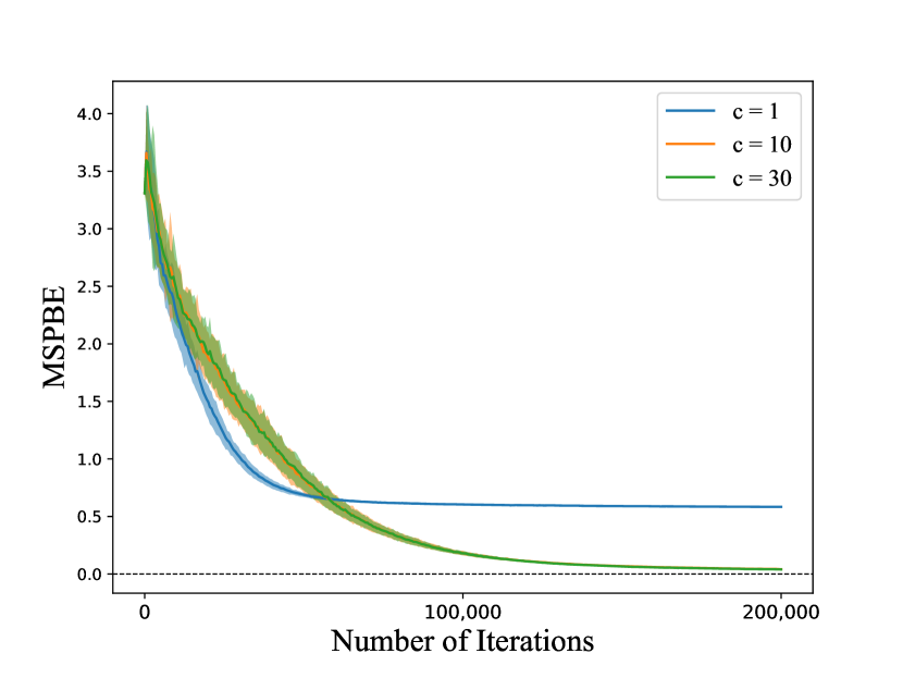
Figure 2: MSPBE of the estimated state-action value functions. The graph shows the average MSPBE ($\pm$ standard deviation) over $100$ runs.

7.2 MountainCar-v0

d	Q-learning	CQL	Double QL	Algorithm 1$,\tau=0.01$	Algorithm 1$,\tau=0.05$
30	$-177.28\pm 32.00$	$-199.37\pm 06.27$	$-177.51\pm 33.73$	$\boldsymbol{-144.36\pm 26.46}$	$-177.83\pm 30.09$
60	$-143.08\pm 32.47$	$-200.00\pm 00.00$	$-132.76\pm 31.54$	$\boldsymbol{-121.01\pm 31.82}$	$-123.84\pm 28.35$
90	$-175.40\pm 17.77$	$-200.00\pm 00.00$	$-146.78\pm 22.74$	$-121.37\pm 19.84$	$\boldsymbol{-120.31\pm 19.20}$
120	$\boldsymbol{-138.74\pm 11.00}$	$-199.12\pm 03.97$	$-146.23\pm 12.77$	$-176.17\pm 22.65$	$-145.15\pm 29.48$
150	$-141.04\pm 24.77$	$-200.00\pm 00.00$	$-155.60\pm 19.43$	$-139.58\pm 20.59$	$\boldsymbol{-120.17\pm 20.64}$
180	$-135.62\pm 32.01$	$-196.32\pm 13.61$	$\boldsymbol{-110.66\pm 20.87}$	$-120.88\pm 22.50$	$-122.64\pm 22.01$

Table 1: Performance of Benchmark Algorithms over 20 Runs.

The MountainCar-v0 environment, a standard control task available in OpenAI Gym [62], challenges an agent to maneuver a car placed between two hills to ascend the hill on the right. The car is characterized by a two-dimensional state space that encompasses its horizontal position and velocity. The agent can choose from three distinct actions at each timestep: accelerate to the left, accelerate to the right, or do nothing. For every timestep that elapses before the car reaches the summit, the agent incurs a reward of $-1$. Consequently, the agent’s objective is to reach the summit as fast as possible to maximize its cumulative reward. Given that the episode is capped at $200$ timesteps, the agent’s return is confined within the range of $[-200,0]$.

We employ Radial Basis Functions (RBFs) as our basis functions and incorporate $l$ Gaussian kernels, each with a width of $1$, randomly selected from the state space. Since each RBF corresponds to three distinct actions, the total number of features is $d=3l$. We set the stepsize parameters to $\alpha=0.1$ and $\beta=0.1$, and the threshold for Algorithm 1 is assigned a value of $\delta=500$. Considering the environment’s finite horizon, we adopt a discount factor of $\gamma=1$.

We evaluated the policies derived from Algorithm 1 with a negative entropy regularizer and compared them with those obtained through Q-learning [14], Coupled Q-learning (CQL) [25], Greedy-GQ [27], and Double Q-learning (Double QL) [35]. We selected the coefficient of the regularizer for Algorithm 1 from the set $\{0.01,0.05\}$. For Algorithm 1, we adopted the regularized policy $\pi_{\theta}$ defined in 4 as the behavioral policy. In contrast, an $\epsilon$-greedy policy, with $\epsilon=0.1$, served as the behavioral policy for the other mentioned algorithms.

Table 1 summarizes the policy performances, with the exception of Greedy-GQ, which consistently registered a return of $-200$ across all testing episodes. Each of the $20$ training phases, differentiated by random seeds, comprised $1,000$ episodes. The table displays the average returns obtained during testing, averaged over $20$ runs, each encompassing $10$ episodes. The results demonstrate that the policies derived from Algorithm 1 outperform those obtained from other algorithms in most cases.

8 Auxiliary Lemmas

Lemma H1

Under Assumptions 3.1 and 3.2, $\omega^{*}(\cdot)$ is Lipschitz with respect to $\theta\in\mathbb{R}^{d}$ with constant $\gamma/\lambda_{g}$.

Proof 8.2.

The gradient of $\omega^{*}(\theta)$ with respect to $\theta\in\mathbb{R}^{d}$ is rl &∇_θω^*(θ)
= γΣ^-1E_D[z(s^′;τ, δ,θ)∑_a^′∈Aπ_θ(a^′∣s^′)ϕ(s,a) ϕ(s^′,a^′)^⊤]. The $\ell_{2}$-norm of the gradient of $\omega^{*}(\theta)$ is bounded as $\left\|\nabla_{\theta}\omega^{*}(\theta)\right\|\leq 1/\lambda_{g}$. According to the mean value theorem, we have rCr ∥ω^*(θ_1)-ω^*(θ_2)∥ &≤max_θ ∥∇_θω^*(θ)∥∥θ_1-θ_2∥
≤1λg ∥θ_1-θ_2∥.

Lemma 8.3.

Under Assumption 3.2, the policy $\pi_{\theta}(\cdot\mid s)$ is Lipschitz in $\theta\in\mathbb{R}^{d}$ with constant $L_{G}\sqrt{|\mathcal{A}|}/\tau$ for $s\in\mathcal{S}$.

Proof 8.4.

By the properties of the regularizer and Assumption 3.2, for $s\in\mathcal{S}$ and $\theta_{1},\theta_{2}\in\mathbb{R}^{d}$, we have rlr ∥π_θ_1(⋅​∣​s)- π_θ_2(⋅​∣​ s)∥ =& ∥∇G^*_τ(^Q_θ_1(s,⋅))-∇G^*_τ(^Q_θ_2(s,⋅)) ∥
≤ LGτ ∥^Q_θ_1(s,⋅)-^Q_θ_2(s,⋅)∥
≤ LG—A—τ ∥θ_1-θ_2∥.

Lemma 8.5.

Under Assumption 3.2, the matrix $\hat{\Sigma}_{\tau,\delta,\theta}$ is Lipschitz in $\theta\in\mathbb{R}^{d}$ with constant $(L_{G}|\mathcal{A}|/\tau+2/\delta)$.

Proof 8.6.

We first derive the Lipschitz property for $\hat{G}_{\tau,\delta}(\hat{Q}_{\theta}(s^{\prime},\cdot))^{2}$ with respect to $\theta$. The derivative of the expression with respect to $\theta$ is given by

$$\nabla_{\theta}\hat{G}^{2}_{\tau,\delta} (\hat{Q}_{\theta}(s^{\prime},\cdot))$$

$$= \nabla_{\theta}\mathcal{K}^{2}_{\delta}(G^{*}_{\tau}(\hat{Q}_{\theta}(s^{\prime},\cdot)))$$

$$= 2\hat{G}_{\tau,\delta}(\hat{Q}_{\theta}(s^{\prime},\cdot))z\left(s^{\prime};\delta,\theta\right)\sum_{a\in\mathcal{A}}\pi_{\theta}(a\mid s)\phi(s,a).$$

The $\ell_{2}$-norm of this derivative is bounded by $2\delta$. Thus, by the mean value theorem, for $s\in\mathcal{S}$ and $\theta_{1},\theta_{2}\in\mathbb{R}^{d}$, we obtain

$$\left\|\hat{G}^{2}_{\tau,\delta}(\hat{Q}_{\theta_{1}}(s^{\prime},\cdot))-\hat{G}^{2}_{\tau,\delta}(\hat{Q}_{\theta_{2}}(s^{\prime},\cdot))\right\|\leq 2\delta\left\|\theta_{1}-\theta_{2}\right\|.$$ (18)

Next, we establish the Lipschitz property for $\hat{\Sigma}_{\tau,\delta,\theta}$. Given the definition of $\hat{\Sigma}_{\tau,\delta,\theta}$ in (3.2), for $\theta_{1},\theta_{2}\in\mathbb{R}^{d}$, we have

$$\| \hat{\Sigma}_{\tau,\delta,\theta_{1}}-\hat{\Sigma}_{\tau,\delta,\theta_{2}}\|$$

$$\leq\left\|\mathbb{E}_{\mathcal{D}}\left[\phi\left(s^{\prime},\cdot\right)\left(\pi_{\theta_{1}}\left(\cdot\mid s^{\prime}\right)-\pi_{\theta_{2}}\left(\cdot\mid s^{\prime}\right)\right)\phi(s,a)^{\top}\right]\right\|$$

$$\ \ \ +\frac{1}{\delta^{2}}\left\|\mathbb{E}_{\mathcal{D}}\left[\hat{G}^{2}_{\tau,\delta}(\hat{Q}_{\theta_{2}}(s^{\prime},\cdot))-\hat{G}^{2}_{\tau,\delta}(\hat{Q}_{\theta_{1}}(s^{\prime},\cdot))\right]\right\|$$

$$\leq\left(\frac{L_{G}|\mathcal{A}|}{\tau}+\frac{2}{\delta}\right)\left\|\theta_{1}-\theta_{2}\right\|,$$

where the last inequality is due to Lemma 8.3 and (18).

Lemma 8.7.

Under Assumption 3.2, two consecutive iterates $\theta^{t}$ and $\theta^{t+1}$ in Algorithm 1 for $t=0,1,\dots,T-1$ satisfy $\|\theta^{t+1}-\theta^{t}\|\leq 2\alpha$.

Proof 8.8.

The proof for the case of $\omega^{t+1}=\theta^{t}$ is trivial, since $\theta^{t+1}=\theta^{t}$. On the other hand, when $\omega^{t+1}\neq\theta^{t}$,

$$\left\|\theta^{t+1}-\theta^{t}\right\|$$

$$\leq\alpha\left\|\gamma z\left(s^{\prime};\tau,\delta,\theta^{t}\right)\sum_{a^{\prime}\in\mathcal{A}}\!\!\pi_{\theta^{t}}\left(a^{\prime}\mid s^{\prime}_{t}\right)\phi(s_{t}^{\prime},a^{\prime})-\phi(s_{t},a_{t})\right\|$$

$$\leq 2\alpha.$$

Lemma 8.9.

Under Assumption 3.2, for $\omega,\theta\in\mathbb{R}^{d}$, the difference between the gradient and the surrogate gradient of $J(\cdot)$ is bounded: $\left\|\nabla J(\theta)-\bar{\nabla}_{\theta}f(\theta,\omega)\right\|\leq 2\left\|\omega^{*}(\theta)-\omega\right\|$.

Proof 8.10.

Given the definitions of the gradient $\nabla J(\theta)$ and the surrogate gradient $\bar{\nabla}_{\theta}f(\theta,\omega)$ in (3.2) and (10b), respectively, we have

$$\|\nabla J(\theta)-\bar{\nabla}_{\theta}f(\theta,\omega)\| \leq\left\|\hat{\Sigma}_{\tau,\delta,\theta}\left(\omega^{*}\left(\theta\right)-\omega\right)\right\|$$

$$\leq\left\|\hat{\Sigma}_{\tau,\delta,\theta}\right\|\,\left\|\omega^{*}\left(\theta\right)-\omega\right\|$$

$$\leq 2\left\|\omega^{*}\left(\theta\right)-\omega\right\|.$$

9 Proofs of Theorems

9.1 Proof of Theorem 5.3

Let $\mathcal{F}_{t}:=\sigma\left\{\omega^{0},\theta^{0},\ldots,\omega^{t},\theta^{t}\right\}$ and $\mathcal{F}^{\prime}_{t}:=\sigma\left\{\omega^{0},\theta^{0},\ldots,\omega^{t},\theta^{t},\omega^{t+1}\right\}$ be the filtration of the random variables up to iteration $t$, where $\sigma\{\cdot\}$ denotes the $\sigma$-algebra generated by the random variables. Similar to the definition in (10a) and (10b), suppose $(\tilde{s},\tilde{a},\tilde{s}^{\prime})\sim\mathcal{D}$, we define $\tilde{h}_{g}^{t}$ and $\tilde{h}_{f}^{t}$ as:

$$\tilde{h}_{g}^{t} \triangleq\phi(\tilde{s},\tilde{a})\Big{(}\phi(\tilde{s},\tilde{a})^{\top}\omega^{t}-R(\tilde{s},\tilde{a})-\gamma\hat{G}_{\tau,\delta}(\hat{Q}_{\theta^{t}}\left(\tilde{s}^{\prime}_{t},\cdot\right))\Big{)},$$

$$\tilde{h}_{f}^{t} \triangleq\bigg{(}\gamma z\left(\tilde{s}^{\prime};\tau,\delta,\theta^{t}\right)\sum_{\tilde{a}^{\prime}\in\mathcal{A}}\pi_{\theta^{t}}\left(\tilde{a}^{\prime}\mid\tilde{s}^{\prime}\right)\phi(\tilde{s}^{\prime},\tilde{a}^{\prime})-\phi(\tilde{s},\tilde{a})\bigg{)}$$

$$\qquad\qquad\qquad\ \ \ \ \ \ \ \ \ \ \ \ \times\phi(\tilde{s},\tilde{a})^{\top}\left(\omega^{t+1}-\theta^{t}\right).$$

It follows that $\mathbb{E}[\tilde{h}_{g}^{t}\mid\mathcal{F}_{t}]=\nabla_{\omega}g(\theta^{t},\omega^{t})$ and $\mathbb{E}[\tilde{h}_{f}^{t}\mid\mathcal{F}_{t}^{\prime}]=\bar{\nabla}_{\omega}f\left(\theta^{t},\omega^{t+1}\right)$. Also, under Assumption 3.1, we define $T_{\alpha}$ as the number of iterations needed to ensure the bias incurred by the Markovian sampling is sufficiently small:

$$T_{\alpha}\triangleq\min\left\{t\in\mathbb{N}^{+}\mid\kappa\rho^{t}\leq\alpha\right\}.$$ (19)

We first start with the error in the lower-level problem. The following lemma demonstrates the tracking error of the estimated main network $\hat{Q}_{\omega^{t}}$.

Lemma 9.1.

(Tracking error). Given the conditions stated in Theorem 5.3,

$$\frac{1}{T}\sum_{t=0}^{T-1}\mathbb{E}\left\|\omega^{*}(\theta^{t})-\omega^{t+1}\right\|^{2}=\mathcal{O}\left(T^{-1/2}\right).$$

See Appendix 10.3 for a detailed proof. As a result, by Jensen’s inequality, we can derive

$$\frac{1}{T}\sum_{t=0}^{T-1}\mathbb{E}\left\|\omega^{*}(\theta^{t})-\omega^{t+1}\right\|\leq \sqrt{\frac{1}{T}\sum_{t=0}^{T-1}\mathbb{E}\left\|\omega^{*}(\theta^{t})-\omega^{t+1}\right\|^{2}}$$

$$= \mathcal{O}\left(T^{-1/4}\right).$$ (20)

Now, we provide the proof for the second bound in Theorem 5.3. Toward this end, we use the following lemma.

Lemma 9.2.

Given the conditions stated in Theorem 5.3,

$$\frac{1}{T}\sum_{t=0}^{T-1}\left\|\bar{\nabla}f\left(\theta^{t},\omega^{t+1}\right)\right\|=\mathcal{O}\left(T^{-1/4}\right).$$

See Appendix 10.4 for a detailed proof.

Finally, it is straightforward to derive (13). By the triangle inequality and Lemma 8.9, we have

$$\frac{1}{T} \sum_{t=0}^{T-1}\left\|{\nabla}J\left(\theta^{t}\right)\right\|$$

$$\leq\frac{1}{T}\sum_{t=0}^{T-1}\left(\left\|{\nabla}J\left(\theta^{t}\right)-\bar{\nabla}f\left(\theta^{t},\omega^{t+1}\right)\right\|+\left\|\bar{\nabla}f\left(\theta^{t},\omega^{t+1}\right)\right\|\right)$$

$$\leq\frac{2}{T}\sum_{t=0}^{T-1}\left\|\omega^{*}\left(\theta^{t}\right)-\omega^{t+1}\right\|+\frac{1}{T}\sum_{t=0}^{T-1}\left\|\bar{\nabla}f\left(\theta^{t},\omega^{t+1}\right)\right\|$$

$$=\mathcal{O}\left(T^{-1/4}\right).$$

The proof is concluded.

9.2 Proof of Theorem 5.7

We start with the first bound in Theorem 5.7. For $t>0$, the triangle inequality yields

$$\|Q^{*}_{\tau}-\hat{Q}_{{\theta^{t}}}\|_{\infty}\leq \|Q^{*}_{\tau}-\mathcal{B}_{\tau,\delta}\hat{Q}_{{\theta^{t}}}\|_{\infty}$$

$$\quad+\|\mathcal{B}_{\tau,\delta}\hat{Q}_{{\theta^{t}}}-\Pi\mathcal{B}_{\tau,\delta}\hat{Q}_{{\theta^{t}}}\|_{\infty}$$

$$\quad\quad+\|\Pi\mathcal{B}_{\tau,\delta}\hat{Q}_{{\theta^{t}}}-\hat{Q}_{{\theta^{t}}}\|_{\infty}.$$ (21)

For the first term in (9.2), due to regularized Bellman equation and the $\gamma$-contraction property of the smooth truncated optimal regularized Bellman operator $\mathcal{B}_{\tau,\delta}$ in $\ell_{\infty}$-norm, we obtain

$$\|Q^{*}_{\tau}-\mathcal{B}_{\tau,\delta}\hat{Q}_{{\theta^{t}}}\|_{\infty}\!\leq \|\mathcal{B}_{\tau}Q^{*}_{\tau}-\mathcal{B}_{\tau,\delta}Q^{*}_{\tau}\|+\gamma\|Q^{*}_{\tau}-\hat{Q}_{{\theta^{t}}}\|_{\infty}$$

$$= \gamma\max_{s\in\mathcal{S}}\left|V_{\tau}^{*}-\mathcal{K}_{\delta}\left(V_{\tau}^{*}\right)\right|+\gamma\|Q^{*}_{\tau}-\hat{Q}_{{\theta^{t}}}\|_{\infty}$$

$$\leq \gamma\left(\delta_{0}-\mathcal{K}_{\delta}\!\left(\delta_{0}\right)\right)+\gamma\|Q^{*}_{\tau}-\hat{Q}_{{\theta^{t}}}\|_{\infty},$$ (22)

where the last inequality follows from the fact $\|V_{\pi,\tau}\|_{\infty}\leq\frac{R_{\max}+\tau B}{1-\gamma}=\delta_{0}$ for any policy $\pi$ and (2). Next, we can bound the second term in (9.2) by the definition of approximation error in (14):

$$\left\|\mathcal{B}_{\tau,\delta}\hat{Q}_{{\theta^{t}}}-\Pi\mathcal{B}_{\tau,\delta}\hat{Q}_{{\theta^{t}}}\right\|_{\infty}\leq\mathcal{E}_{\mathrm{approx}}.$$ (23)

Finally, we bound the last term in (9.2). Under Assumption 3.4 and given the expression of $\nabla J(\cdot)$, we have

$$\left\|\theta^{t}-\omega^{*}\left(\theta\right)\right\|\leq\frac{1}{\sigma_{\min}}\left\|\nabla J\left(\theta^{t}\right)\right\|$$

Then, provided the equation $\hat{Q}_{\omega^{*}\left(\theta\right)}=\Pi\mathcal{B}_{\tau,\delta}\hat{Q}_{\theta}$, we obtain

$$\left\|\Pi\mathcal{B}_{\tau,\delta}\hat{Q}_{{\theta^{t}}}-\hat{Q}_{{\theta^{t}}}\right\|_{\infty}= \left\|\hat{Q}_{\omega^{*}\left(\theta^{t}\right)}-\hat{Q}_{{\theta^{t}}}\right\|_{\infty}$$

$$= \left\|\Phi\omega^{*}\left(\theta^{t}\right)-\Phi\theta^{t}\right\|_{\infty}$$

$$= \max_{(s,a)\in\mathcal{S}\times\mathcal{A}}\left|\phi(s,a)^{\top}\left(\omega^{*}\left(\theta^{t}\right)-\theta^{t}\right)\right|$$

$$\leq \left\|\omega^{*}\left(\theta^{t}\right)-\theta^{t}\right\|$$

$$\leq \frac{1}{\sigma_{\min}}\left\|\nabla J\left(\theta^{t}\right)\right\|.$$ (24)

Substituting (9.2), (23) and (9.2) into (9.2) leads to

$$(1-\gamma) \|Q^{*}_{\tau}-\hat{Q}_{{\theta^{t}}}\|_{\infty}$$

$$\leq \frac{1}{\sigma_{\min}}\|\nabla J\left(\theta^{t}\right)\|+\gamma\left(\delta_{0}-\mathcal{K}_{\delta}\left(\delta_{0}\right)\right)+\mathcal{E}_{\mathrm{approx}}.$$

Taking full expectation and summing from $t=0$ to $t=T-1$ for the above inequality completes the proof of (5.7).

For the second bound in Theorem 5.7, given the definition of $V_{\tau}^{t}$, we have

$$\mathbb{E}\|V^{*}_{\tau}- V_{\pi_{\theta^{t}},\tau}\|_{\infty}$$

$$\leq \mathbb{E}\left[\max_{s\in\mathcal{S}}\left|V^{*}_{\tau}(s)-G^{*}_{\tau}(\hat{Q}_{\theta^{t}}\left(s,\cdot\right))\right|\right]$$

$$+\mathbb{E}\left[\max_{s\in\mathcal{S}}\left|G^{*}_{\tau}(\hat{Q}_{\theta^{t}}\left(s,\cdot\right))-V_{\pi_{\theta^{t}},\tau}(s)\right|\right].$$ (25)

For the first term in (9.2), we utilize the properties of the convex conjugate $G^{*}$ of the regularizer:

$$\max_{s\in\mathcal{S}} \left|V^{*}_{\tau}(s)-G^{*}_{\tau}\left(\hat{Q}_{\theta^{t}}\left(s,\cdot\right)\right)\right|$$

$$=\max_{s\in\mathcal{S}}\left|G^{*}_{\tau}\left({Q}^{*}_{G,\tau}\left(s,\cdot\right)\right)-G^{*}_{\tau}\left(\hat{Q}_{\theta^{t}}\left(s,\cdot\right)\right)\right|$$

$$\leq\max_{s\in\mathcal{S}}\max_{q\in\mathbb{R^{|\mathcal{A}|}}}\left|\nabla G^{*}(q)^{\top}\left(Q^{*}_{\tau}(s,\cdot)-\hat{Q}_{{\theta^{t}}}(s,\cdot)\right)\right|$$

$$\leq\max_{s\in\mathcal{S}}\max_{a\in\mathcal{A}}\left|Q^{*}_{\tau}(s,a)-\hat{Q}_{{\theta^{t}}}(s,a)\right|$$

$$=\left\|Q^{*}_{\tau}-\hat{Q}_{{\theta^{t}}}\right\|_{\infty},$$ (26)

where the first inequality follows from Taylor’s theorem and the second inequality is due to Proposition 2.1.

For the second term in (9.2), the bound can be developed similarly. Given definition of $\pi_{\theta}$ in (4), for $s\in\mathcal{S}$, we have

$$G^{*}_{\tau}(\hat{Q}_{\theta^{t}}\left(s,\cdot\right))= \max_{p\in\Delta(\mathcal{A})}\sum_{a}p(a)\,\hat{Q}_{{\theta^{t}}}(s,a)-G_{\tau}\left(p\right)$$

$$= \sum_{a}\pi_{\theta^{t}}(a\mid s)\,\hat{Q}_{{\theta^{t}}}(s,a)-G_{\tau}\left(\pi_{\theta^{t}}(\cdot\mid s)\right).$$

Therefore, by the definition of $V_{\pi,\tau}$ and $Q_{\pi,\tau}$, we can derive the bound

$$\max_{s\in\mathcal{S}} \left|G^{*}_{\tau}(\hat{Q}_{\theta^{t}}\left(s,\cdot\right))-V_{\pi_{\theta^{t}},\tau}(s)\right|$$

$$=\max_{s\in\mathcal{S}}\Bigg{|}\sum_{a}\pi_{\theta^{t}}(a\mid s)\hat{Q}_{{\theta^{t}}}(s,a)-G_{\tau}\left(\pi_{\theta^{t}}(\cdot\mid s)\right)$$

$$\quad-\left(\sum_{a}\pi_{\theta^{t}}(a\mid s)Q_{\pi_{\theta^{t}},\tau}(s,a)-G_{\tau}\left(\pi_{\theta^{t}}(\cdot\mid s)\right)\right)\Bigg{|}$$

$$\leq\left\|\hat{Q}_{{\theta^{t}}}-Q_{\pi_{\theta^{t}},\tau}\right\|_{\infty}$$

$$\leq\left\|Q_{\pi_{\theta^{t}},\tau}-\mathcal{B}_{\tau,\delta}\hat{Q}_{\theta^{t}}\right\|_{\infty}+\left\|\mathcal{B}_{\tau,\delta}\hat{Q}_{\theta^{t}}-\Pi\mathcal{B}_{\tau,\delta}\hat{Q}_{\theta^{t}}\right\|_{\infty}$$

$$\quad+\left\|\Pi\mathcal{B}_{\tau,\delta}\hat{Q}_{\theta^{t}}-\hat{Q}_{\theta^{t}}\right\|_{\infty}.$$ (27)

Here, our focus is on providing a bound for the first term, as bounds for the second and third terms have already been established in (23) and (9.2). Given the regularized Bellman equation, we can derive

$$\| Q_{\pi_{\theta^{t}},\tau}-\mathcal{B}_{\tau,\delta}\hat{Q}_{\theta^{t}}\|_{\infty}$$

$$=\gamma\max_{s,a}\left|\mathbb{E}_{s^{\prime}\sim P(\cdot\mid s,a)}\left[{V}_{\pi_{\theta^{t}},\tau}\left(s^{\prime}\right)-\hat{G}_{\tau,\delta}\left(\hat{Q}_{\theta^{t}}\left(s^{\prime},\cdot\right)\right)\right]\right|$$

$$\leq\gamma\max_{s,a}\Big{|}\mathbb{E}_{s^{\prime}\sim P(\cdot\mid s,a)}\Big{[}{V}_{\pi_{\theta^{t}},\tau}\left(s^{\prime}\right)-\mathcal{K}_{\delta}\left({V}_{\pi_{\theta^{t}},\tau}\left(s^{\prime}\right)\right)$$

$$\ \ \ +\mathcal{K}_{\delta}\left({V}_{\pi_{\theta^{t}},\tau}\left(s^{\prime}\right)\right)-\hat{G}_{\tau,\delta}\left(\hat{Q}_{\theta^{t}}\left(s^{\prime},\cdot\right)\right)\Big{]}\Big{|}$$

$$\leq\gamma\left(\delta_{0}-\mathcal{K}_{\delta}\left(\delta_{0}\right)\right)$$

$$\ \ \ +\gamma\max_{s\in\mathcal{S}}\left|{V}_{\pi_{\theta^{t}},\tau}\left(s\right)-G^{*}_{\tau}\left(\hat{Q}_{\theta^{t}}\left(s,\cdot\right)\right)\right|,$$ (28)

where the last inequality follows from the $1$-Lipschitz property of $\mathcal{K}_{\delta}$. Substituting (9.2), (23) and (9.2) into (9.2) leads to

$$\left(1-\gamma\right) \max_{s\in\mathcal{S}}\left|G^{*}_{\tau}(\hat{Q}_{\theta^{t}}\left(s,\cdot\right))-V_{\pi_{\theta^{t}},\tau}(s)\right|$$

$$\leq\frac{1}{\sigma_{\min}}\left\|\nabla J\left(\theta^{t}\right)\right\|+\mathcal{E}_{\mathrm{approx}}+\gamma\left(\delta_{0}-\mathcal{K}_{\delta}\left(\delta_{0}\right)\right).$$

Combining the above inequality with (9.2) and using the result in (5.7) complete the proof of Theorem 5.7.

10 Proofs of Other Lemmas

10.1 Proof of Lemma 5.1

We first prove the first inequality in Lemma 5.1. By the expression of $\nabla J$ in (3.2), for $\theta_{1},\theta_{2}\in\mathbb{R}^{d}$, we have

$$\|\nabla J\left(\theta_{1}\right)-\nabla J\left(\theta_{2}\right)\|$$

$$= \left\|\hat{\Sigma}_{\tau,\delta,\theta_{1}}\left(\omega^{*}\left(\theta_{1}\right)-\theta_{1}\right)-\hat{\Sigma}_{\tau,\delta,\theta_{2}}\left(\omega^{*}\left(\theta_{2}\right)-\theta_{2}\right)\right\|$$

$$\leq \left\|\hat{\Sigma}_{\tau,\delta,\theta_{1}}\right\|\left\|\omega^{*}\left(\theta_{1}\right)-\theta_{1}-\omega^{*}\left(\theta_{2}\right)+\theta_{2}\right\|$$

$$+\left\|\hat{\Sigma}_{\tau,\delta,\theta_{1}}-\hat{\Sigma}_{\tau,\delta,\theta_{2}}\right\|\left\|\omega^{*}\left(\theta_{2}\right)-\theta_{2}\right\|$$

$$\leq \left\|\hat{\Sigma}_{\tau,\delta,\theta_{1}}\right\|\left(\left\|\omega^{*}\left(\theta_{1}\right)-\omega^{*}\left(\theta_{2}\right)\right\|+\left\|\theta_{1}-\theta_{2}\right\|\right)$$

$$+\left\|\hat{\Sigma}_{\tau,\delta,\theta_{1}}-\hat{\Sigma}_{\tau,\delta,\theta_{2}}\right\|\left\|\omega^{*}\left(\theta_{2}\right)-\theta_{2}\right\|$$

$$\leq \frac{2}{\lambda_{g}}\left\|\hat{\Sigma}_{\tau,\delta,\theta_{1}}\right\|\left\|\theta_{1}-\theta_{2}\right\|$$

$$+\left(\frac{L_{G}|\mathcal{A}|}{\tau}+\frac{2}{\delta}\right)\left\|\omega^{*}\left(\theta_{2}\right)-\theta_{2}\right\|\left\|\theta_{1}-\theta_{2}\right\|$$

$$\leq \left(\frac{4}{\lambda_{g}}+\left(\frac{L_{G}|\mathcal{A}|}{\tau}+\frac{2}{\delta}\right)\left\|\omega^{*}\left(\theta_{2}\right)-\theta_{2}\right\|\right)\left\|\theta_{1}-\theta_{2}\right\|,$$

where the third inequality is due to Lemma H1 and Lemma 8.5, and the last inequality follows from the definition of $\hat{\Sigma}_{\tau,\delta,\theta}$ in (3.2).

For the second inequality in Lemma 5.1, we utilize the integral remainder term from the Taylor expansion and the preceding inequality:

$$J\left(\theta_{1}\right) -J\left(\theta_{2}\right)-\left\langle\nabla J\left(\theta_{2}\right),\theta_{1}-\theta_{2}\right\rangle$$

$$= \int_{0}^{1}\left\langle\nabla J\left(\xi\theta_{1}+\left(1-\xi\right)\theta_{2}\right)-\nabla J(\theta_{2}),\theta_{1}-\theta_{2}\right\rangle d\xi$$

$$\leq \int_{0}^{1}\left\|\nabla J\left(\xi\theta_{1}+\left(1-\xi\right)\theta_{2}\right)-\nabla J(\theta_{2})\right\|d\xi\cdot\left\|\theta_{1}-\theta_{2}\right\|$$

$$\leq \int_{0}^{1}\xi d\xi\cdot\left(L_{0}+L_{1}\left\|\omega^{*}\left(\theta_{2}\right)-\theta_{2}\right\|\right)\left\|\theta_{1}-\theta_{2}\right\|^{2}$$

$$= \frac{L_{0}+L_{1}\left\|\omega^{*}\left(\theta_{2}\right)-\theta_{2}\right\|}{2}\left\|\theta_{1}-\theta_{2}\right\|^{2}.$$

This completes the proof.

10.2 Proof of Lemma 5.2

By the definition of $h_{g}^{t}$ in (10a), we have

$$\left\|h_{g}^{t}\right\|= \Big{\|}\phi(s_{t},a_{t})\!\big{(}\phi(s_{t},a_{t})^{\!\top}\!\omega^{t}\!-\!R(s_{t},a_{t})\!-\!\gamma\hat{G}_{\tau,\delta}(\hat{Q}_{\theta^{t}}\!\left(s^{\prime}_{t},\cdot\right))\!\big{)}\!\Big{\|}$$

$$\leq \left\|\omega^{t}\right\|+R_{\max}+\delta$$

$$\leq \frac{2\left(R_{\max}+\delta\right)}{\lambda_{g}},$$

where the last inequality is due to the projection operator in the update (11a) and the fact $\lambda_{g}\leq 1$.

10.3 Proof of Lemma 9.1

For $t\geq T_{\alpha}$, following the update of $\omega^{t+1}$ in (11a) and taking the conditional expectation given filtration $\mathcal{F}_{t}$ yields

$$\mathbb{E} \left[\left\|\omega^{*}(\theta^{t})-\omega^{t+1}\right\|^{2}\mid\mathcal{F}_{t}\right]$$

$$\leq\mathbb{E}\left[\left\|\omega^{*}\left(\theta^{t}\right)-\omega^{t}+\beta h_{g}^{t}\right\|^{2}\mid\mathcal{F}_{t}\right]$$

$$=\left\|\omega^{*}\left(\theta^{t}\right)-\omega^{t}\right\|^{2}$$

$$\quad+\mathbb{E}\Big{[}2\beta\left\langle\omega^{*}\left(\theta^{t}\right)-\omega^{t},\tilde{h}_{g}^{t}-\tilde{h}_{g}^{t}+h_{g}^{t}\right\rangle+\beta^{2}\left\|h_{g}^{t}\right\|^{2}\mid\mathcal{F}_{t}\Big{]}$$

$$=\left\|\omega^{*}\left(\theta^{t}\right)-\omega^{t}\right\|^{2}+2\beta\left\langle\omega^{*}\left(\theta^{t}\right)-\omega^{t},\nabla_{\omega}g(\theta^{t},\omega^{t})\right\rangle$$

$$\quad+2\beta\left\langle\omega^{*}\left(\theta^{t}\right)-\omega^{t},\mathbb{E}\left[h_{g}^{t}-\tilde{h}_{g}^{t}\mid\mathcal{F}_{k}\right]\right\rangle$$

$$\quad\quad+\beta^{2}\mathbb{E}\left[\left\|h_{g}^{t}\right\|^{2}\mid\mathcal{F}_{t}\right]$$

$$\leq 2\beta\left(g(\theta^{t},\omega^{*}\left(\theta^{t}\right))-g(\theta^{t},\omega^{t})\right)$$

$$\ \ \ \ \ \ +(1-\beta\lambda_{g})\left\|\omega^{*}\left(\theta^{t}\right)-\omega^{t}\right\|^{2}$$

$$\quad\quad\quad+2\beta\left\langle\omega^{*}\left(\theta^{t}\right)-\omega^{t},\mathbb{E}\left[h_{g}^{t}-\tilde{h}_{g}^{t}\mid\mathcal{F}_{k}\right]\right\rangle$$

$$\quad\quad\quad\quad+\beta^{2}\mathbb{E}\left[\left\|h_{g}^{t}\right\|^{2}\mid\mathcal{F}_{t}\right]$$

$$\leq(1-\beta\lambda_{g})\|\omega^{*}\left(\theta^{t}\right)-\omega^{t}\|^{2}$$

$$\quad+2\beta\left\langle\omega^{*}\left(\theta^{t}\right)-\omega^{t},\mathbb{E}\left[h_{g}^{t}-\tilde{h}_{g}^{t}\mid\mathcal{F}_{k}\right]\right\rangle$$

$$\quad\quad+\beta^{2}\mathbb{E}\left[\left\|h_{g}^{t}\right\|^{2}\mid\mathcal{F}_{t}\right],$$ (29)

where the first inequality follows from the property of the projection $\mathcal{P}$ and the third inequality is due to Proposition 3.3.

We first analyze the first term in (10.3). If $\beta\geq 1/\lambda_{g}$, this term can be upper bounded by $0$ and the subsequent results are easy to derive. If otherwise, meaning $\beta<1/\lambda_{g}$, we have

$$(1-\beta\lambda_{g})\|\omega^{*}\left(\theta^{t}\right)-\omega^{t}\|^{2}$$

$$=\left(1-\beta\lambda_{g}\right)\left\|\omega^{*}\left(\theta^{t}\right)-\omega^{*}(\theta^{t-1})+\omega^{*}(\theta^{t-1})-\omega^{t}\right\|^{2}$$

$$\leq\left(1-\beta\lambda_{g}\right)\left(1+c\right)\left\|\omega^{*}\left(\theta^{t}\right)-\omega^{*}(\theta^{t-1})\right\|^{2}$$

$$\ \ \ \ \ \ +\left(1-\beta\lambda_{g}\right)\left(1+\frac{1}{c}\right)\left\|\omega^{*}(\theta^{t-1})-\omega^{t}\right\|^{2}$$

$$\leq\left(1-\beta\lambda_{g}\right)\left((1+c)\frac{4\alpha^{2}}{\lambda_{g}^{2}}+\left(1+\frac{1}{c}\right)\left\|\omega^{*}(\theta^{t-1})-\omega^{t}\right\|^{2}\right)$$

$$\leq\frac{8\alpha^{2}}{\beta\lambda_{g}^{3}}+\left(1-\frac{\beta\lambda_{g}}{2}\right)\left\|\omega^{*}(\theta^{t-1})-\omega^{t}\right\|^{2},$$ (30)

where the first inequality is due to Young’s inequality (and holds for any $c>0$), the second one follows from combining Lemma H1 and Lemma 8.7, and the last one is obtained by setting $c=\frac{2(1-\beta\lambda_{g})}{\beta\lambda_{g}}$.

For the second term in (10.3), we can bound it as:

$$\left\langle\omega^{*}\left(\theta^{t}\right)-\omega^{t},\mathbb{E}\left[h_{g}^{t}-\tilde{h}_{g}^{t}\mid\mathcal{F}_{k}\right]\right\rangle$$

$$\quad\leq\left\|\omega^{*}\left(\theta^{t}\right)-\omega^{t}\right\|\cdot\left\|\mathbb{E}\left[h_{g}^{t}-\tilde{h}_{g}^{t}\mid\mathcal{F}_{k}\right]\right\|$$

$$\quad\leq\frac{2\left(R_{\max}+\delta\right)}{\lambda_{g}}\left\|\mathbb{E}\left[h_{g}^{t}-\tilde{h}_{g}^{t}\mid\mathcal{F}_{k}\right]\right\|$$

$$\quad\leq\frac{4\left(R_{\max}+\delta\right)^{2}}{\lambda_{g}^{2}}$$

$$\quad\quad\times d_{TV}\left(\mathbb{P}\left(\left(s_{t},a_{t},s_{t}^{\prime}\right)\in\cdot\mid s_{0}\sim\mu_{0},\pi_{\mathrm{bhv}},P\right),\mathcal{D}\right)$$

$$\quad\leq\frac{4\alpha\left(R_{\max}+\delta\right)^{2}}{\lambda_{g}^{2}},$$ (31)

where the third inequality follows the definition of the total-variation norm and Lemma 5.2, and the last inequality uses Lemma 1 in [48].

The last term in (10.3) can be bounded by Lemma 5.2 as

$$\mathbb{E}\left[\left\|h_{g}^{t}\right\|^{2}\mid\mathcal{F}_{k}\right]\leq\frac{4\left(R_{\max}+\delta\right)^{2}}{\lambda_{g}^{2}}.$$ (32)

Substituting (10.3), (10.3) and (32) into (10.3) yields

$$\mathbb{E} \left[\left\|\omega^{*}(\theta^{t})-\omega^{t+1}\right\|^{2}\mid\mathcal{F}_{t}\right]$$

$$\quad\quad\leq\left(1-\frac{\beta\lambda_{g}}{2}\right)\left\|\omega^{*}(\theta^{t-1})-\omega^{t}\right\|^{2}+\frac{8\alpha^{2}}{\beta\lambda_{g}^{3}}$$

$$\quad\quad\quad\quad+\frac{\left(8\alpha\beta+4\beta^{2}\right)\left(R_{\max}+\delta\right)^{2}}{\lambda_{g}^{2}}.$$ (33)

Taking the full expectation of the above inequality and summing it from $t=T_{\alpha}+1$ to $t=T$ gives

$$\sum_{t=T_{\alpha}+1}^{T}\mathbb{E} \left\|\omega^{*}(\theta^{t})-\omega^{t+1}\right\|^{2}$$

$$\leq \left(1-\frac{\beta\lambda_{g}}{2}\right)\sum_{t=T_{\alpha}+1}^{T}\mathbb{E}\left\|\omega^{*}(\theta^{t-1})-\omega^{t}\right\|^{2}+\frac{8T\alpha^{2}}{\beta\lambda_{g}^{3}}$$

$$\quad+\frac{\left(8T\alpha\beta+4T\beta^{2}\right)\left(R_{\max}+\delta\right)^{2}}{\lambda_{g}^{2}}.$$

Rearranging the above equality leads to

$$\frac{1}{T}\sum_{t=T_{\alpha}}^{T-1}\mathbb{E} \left\|\omega^{*}(\theta^{t})-\omega^{t+1}\right\|^{2}$$

$$\leq\frac{2}{\beta\lambda_{g}T}\mathbb{E}\left\|\omega^{*}(\theta^{T_{\alpha}})-\omega^{T_{\alpha}+1}\right\|^{2}+\frac{16\alpha^{2}}{\beta^{2}\lambda_{g}^{4}}$$

$$\qquad+\frac{\left(16\alpha+8\beta\right)\left(R_{\max}+\delta\right)^{2}}{\lambda_{g}^{3}}$$

$$\leq\frac{8\left(R_{\max}+\delta\right)^{2}}{T\beta\lambda_{g}^{3}}+\frac{16\alpha^{2}}{\beta^{2}\lambda_{g}^{4}}$$

$$\qquad+\frac{\left(16\alpha+8\beta\right)\left(R_{\max}+\delta\right)^{2}}{\lambda_{g}^{3}}.$$ (34)

Given the definition of $T_{\alpha}$ in (19) and the choice of $\alpha$, we obtain $T_{\alpha}=\mathcal{O}\left(\log T\right)$. Thus, we can derive

$$\sum_{t=0}^{T_{\alpha}-1}\mathbb{E}\left\|\omega^{*}(\theta^{t})-\omega^{t+1}\right\|^{2}\leq T_{\alpha}\cdot\frac{4\left(R_{\max}+\delta\right)^{2}}{\lambda_{g}^{2}}$$

$$= \mathcal{O}\left(\log T\right).$$ (35)

Combining (10.3) and (10.3) yields

$$\frac{1}{T}\sum_{t=0}^{T-1} \mathbb{E}\left\|\omega^{*}(\theta^{t})-\omega^{t+1}\right\|^{2}$$

$$\leq \mathcal{O}\left(\frac{\log T}{T}\right)+\frac{8\left(R_{\max}+\delta\right)^{2}}{T^{1/2}\beta_{0}\lambda_{g}^{3}}+\frac{16\alpha_{0}^{2}}{T^{1/2}\beta_{0}^{2}\lambda_{g}^{4}}$$

$$+\frac{16\alpha_{0}\left(R_{\max}+\delta\right)^{2}}{T^{3/4}\lambda_{g}^{3}}+\frac{8\beta_{0}\left(R_{\max}+\delta\right)^{2}}{T^{1/2}\lambda_{g}^{3}}$$

$$= \mathcal{O}\left(T^{-1/2}\right).$$

10.4 Proof of Lemma 9.2

We first consider the case of $\omega^{t+1}\neq\theta^{t}$. By Lemma 5.1, for $t\geq T_{\alpha}$, we have

$$J\left(\theta^{t+1}\right)-J\left(\theta^{t}\right)\leq \left\langle\nabla J\left(\theta^{t}\right),\theta^{t+1}-\theta^{t}\right\rangle$$

$$+\frac{L_{0}+L_{1}\left\|\omega^{*}\left(\theta^{t}\right)-\theta^{t}\right\|}{2}\left\|\theta^{t+1}-\theta^{t}\right\|^{2}$$

$$\leq \left\langle\nabla J\left(\theta^{t}\right),-\frac{\alpha}{\|\omega^{t+1}-\theta^{t}\|}{h}_{f}^{t}\right\rangle$$

$$+2\alpha^{2}L_{0}+2\alpha^{2}L_{1}\left\|\omega^{*}\left(\theta^{t}\right)-\theta^{t}\right\|$$

$$\leq \left\langle\nabla J\left(\theta^{t}\right),-\frac{\alpha}{\|\omega^{t+1}-\theta^{t}\|}\tilde{h}_{f}^{t}\right\rangle$$

$$+\left\langle\nabla J\left(\theta^{t}\right),-\frac{\alpha}{\|\omega^{t+1}-\theta^{t}\|}\left(h_{f}^{t}-\tilde{h}_{f}^{t}\right)\right\rangle$$

$$+2\alpha^{2}L_{0}+2\alpha^{2}L_{1}\left\|\omega^{*}\left(\theta^{t}\right)-\theta^{t}\right\|,$$ (36)

where the second inequality follows from Lemma 8.7. We first focus on the first term on the right-hand side (10.4). By taking the conditional expectation on $\mathcal{F}^{\prime}_{t}$, it becomes

$$\mathbb{E}\left[\left\langle\nabla J\left(\theta^{t}\right),-\frac{\alpha}{\|\omega^{t+1}-\theta^{t}\|}\tilde{h}_{f}^{t}\right\rangle\mid\mathcal{F}^{\prime}_{t}\right]$$

$$= \left\langle\nabla J\left(\theta^{t}\right),-\frac{\alpha}{\|\omega^{t+1}-\theta^{t}\|}\bar{\nabla}f(\theta^{t},\omega^{t+1})\right\rangle$$

$$= \bigg{\langle}\nabla J\left(\theta^{t}\right)-\bar{\nabla}f\left(\theta^{t},\omega^{t+1}\right),-\frac{\alpha}{\|\omega^{t+1}-\theta^{t}\|}\bar{\nabla}f\left(\theta^{t},\omega^{t+1}\right)\bigg{\rangle}$$

$$+\left\langle\bar{\nabla}f\left(\theta^{t},\omega^{t+1}\right),-\frac{\alpha}{\|\omega^{t+1}-\theta^{t}\|}\bar{\nabla}f\left(\theta^{t},\omega^{t+1}\right)\right\rangle$$

$$\leq \alpha\left\|\nabla J\left(\theta^{t}\right)-\bar{\nabla}f\left(\theta^{t},\omega^{t+1}\right)\right\|\frac{\left\|\bar{\nabla}f\left(\theta^{t},\omega^{t+1}\right)\right\|}{\|\omega^{t+1}-\theta^{t}\|}$$

$$-\frac{\alpha}{\|\omega^{t+1}-\theta^{t}\|}\left\|\bar{\nabla}f\left(\theta^{t},\omega^{t+1}\right)\right\|^{2}$$

$$\leq 4\alpha\left\|\omega^{*}\left(\theta^{t}\right)-\omega^{t+1}\right\|-\frac{\alpha\left\|\bar{\nabla}f\left(\theta^{t},\omega^{t+1}\right)\right\|^{2}}{\|\omega^{t+1}-\theta^{t}\|},$$ (37)

where the last inequality is due to Lemma 8.9. Under Assumption 3.4, the $\ell_{2}$-norm of the surrogate gradient is lower bounded as

$$\left\|\bar{\nabla}f\left(\theta^{t},\omega^{t+1}\right)\right\|\geq\sigma_{\min}\left\|\omega^{t+1}-\theta^{t}\right\|.$$ (38)

Thus we can bound (10.4) as

$$\mathbb{E} \left[\left\langle\nabla J\left(\theta^{t}\right),-\frac{\alpha}{\|\omega^{t+1}-\theta^{t}\|}\cdot\tilde{h}_{f}^{t}\right\rangle\mid\mathcal{F}^{\prime}_{t}\right]$$

$$\leq 4\alpha\left\|\omega^{*}\left(\theta^{t}\right)-\omega^{t+1}\right\|-\alpha\sigma_{\min}\left\|\bar{\nabla}f\left(\theta^{t},\omega^{t+1}\right)\right\|.$$ (39)

Next, we analyze the second term on the right-hand side in (10.4). By taking the conditional expectation on $\mathcal{F}_{t}^{\prime}$, we obtain

$$\mathbb{E}\left[\left\langle\nabla J\left(\theta^{t}\right),-\frac{\alpha}{\|\omega^{t+1}-\theta^{t}\|}\left(h_{f}^{t}-\tilde{h}_{f}^{t}\right)\right\rangle\mid\mathcal{F}^{\prime}_{t}\right]$$

$$\leq \alpha\left\|\nabla J\left(\theta^{t}\right)\right\|\frac{\left\|\mathbb{E}\left[h_{f}^{t}-\tilde{h}_{f}^{t}\mid\mathcal{F}^{\prime}_{t}\right]\right\|}{\|\omega^{t+1}-\theta^{t}\|}$$

$$\leq \alpha\left\|\nabla J\left(\theta^{t}\right)\right\|d_{TV}\left(\mathbb{P}\left(\left(s_{t},a_{t},s_{t}^{\prime}\right)\in\cdot\mid s_{0}\sim\mu_{0},\pi_{\mathrm{bhv}},P\right),\mathcal{D}\right)$$

$$\times\sup_{s,a,s^{\prime}}\|(\gamma z\left(s^{\prime};\tau,\delta,\theta^{t}\right)\sum_{a^{\prime}\in\mathcal{A}}\pi_{\theta^{t}}\left(a^{\prime}\mid s^{\prime}\right)\phi(s^{\prime},a^{\prime})-\phi(s,a))\|$$

$$\leq 2\alpha\left\|\nabla J\left(\theta^{t}\right)\right\|d_{TV}\left(\mathbb{P}\left(\left(s_{t},a_{t},s_{t}^{\prime}\right)\in\cdot\mid s_{0}\sim\mu_{0},\pi_{\mathrm{bhv}},P\right),\mathcal{D}\right)$$

$$\leq 2\alpha^{2}\left\|\nabla J\left(\theta^{t}\right)\right\|$$

$$\leq 2\alpha^{2}\left\|\bar{\nabla}_{\theta}f\left(\theta^{t},\omega^{t+1}\right)\right\|+4\alpha^{2}\left\|\omega^{*}\left(\theta^{t}\right)-\omega^{t+1}\right\|,$$ (40)

where the second inequality follows the definition of the total-variation norm and the fourth inequality uses Lemma 1 in [48]. The last inequality is due to Lemma 8.9.

For the third term in (10.4), we bound it by leveraging Assumption 3.4. Given the triangle inequality, we can derive

$$\left\|\omega^{*}\left(\theta^{t}\right)-\theta^{t}\right\|\leq \left\|\omega^{*}\left(\theta^{t}\right)-\omega^{t+1}\right\|+\left\|\theta^{t}-\omega^{t+1}\right\|$$

$$\leq \left\|\omega^{*}\left(\theta^{t}\right)-\omega^{t+1}\right\|+\frac{\left\|\bar{\nabla}f\left(\theta^{t},\omega^{t+1}\right)\right\|}{\sigma_{\min}},$$

where the last inequality follows from (38). Taking full expectation in (10.4) and plugging (10.4), (10.4) and the preceding inequality yield

$$\mathbb{E} J\left(\theta^{t+1}\right)-\mathbb{E}J\left(\theta^{t}\right)$$

$$\leq\alpha\left(\alpha\left(\frac{2L_{1}}{\sigma_{\min}}+2\right)-\sigma_{\min}\right)\mathbb{E}\left\|\bar{\nabla}f\left(\theta^{t},\omega^{t+1}\right)\right\|$$

$$\ \ \ +2\alpha\left(2+\alpha^{2}L_{1}+2\alpha\right)\mathbb{E}\left\|\omega^{*}\left(\theta^{t}\right)-\omega^{t+1}\right\|+2\alpha^{2}L_{0}.$$

Observe that the above inequality also holds for the case of $\omega^{t+1}=\theta^{t}$.

Let $\eta\triangleq\sigma_{\min}-\alpha({2L_{1}}/{\sigma_{\min}}+2)$. Given the conditions $\alpha<\frac{\sigma_{\min}^{2}}{2(L_{1}+\sigma_{\min})}$ and $\sigma_{\min}\leq 1$, we can derive

$$\mathbb{E}J\left(\theta^{t+1}\right)-\mathbb{E}J\left(\theta^{t}\right)\leq -\alpha\eta\mathbb{E}\left\|\bar{\nabla}f\left(\theta^{t},\omega^{t+1}\right)\right\|$$

$$+6\alpha\mathbb{E}\left\|\omega^{*}\left(\theta^{t}\right)-\omega^{t+1}\right\|+2\alpha^{2}L_{0}.$$ (41)

Summing it from $t=T_{\alpha}$ to $t=T-1$ gives

$$\!\!\!\!\!\alpha\eta\sum_{t=T_{\alpha}}^{T-1}\mathbb{E}\left\|\bar{\nabla}f\left(\theta^{t},\omega^{t+1}\right)\right\|$$

$$\leq \mathbb{E}J\left(\theta^{T_{\alpha}}\right)+6\alpha\sum_{t=T_{\alpha}}^{T-1}\mathbb{E}\left\|\omega^{*}\left(\theta^{t}\right)-\omega^{t+1}\right\|+2\alpha^{2}TL_{0}.$$ (42)

To continue, we consider the first term in (10.4). By the triangle inequality and Lemma 8.7, we have

$$\left\|\theta^{T_{\alpha}}\right\|\leq \sum_{t=0}^{T_{\alpha}-1}\left\|\theta^{t+1}-\theta^{t}\right\|+\left\|\theta^{0}\right\|$$

$$\leq 2\alpha T_{\alpha}+\left\|\theta^{0}\right\|.$$

Given the definition of the objective function $J$ in (3), we obtain

$$\mathbb{E}J\left(\theta^{T_{\alpha}}\right)\leq \left\|\omega^{*}\left(\theta^{T_{\alpha}}\right)-\theta^{T_{\alpha}}\right\|^{2}$$

$$\leq 2\left\|\omega^{*}\left(\theta^{T_{\alpha}}\right)\right\|^{2}+2\left\|\theta^{T_{\alpha}}\right\|^{2}$$

$$\leq \frac{2\left(R_{\max}+\delta\right)^{2}}{\lambda_{g}^{2}}+16\alpha^{2}T_{\alpha}^{2}+4\left\|\theta^{0}\right\|^{2},$$ (43)

where the last two inequalities follow from Young’s inequality.

For the second term in (10.4), we bound it by using (9.1):

$$\sum_{t=T_{\alpha}}^{T-1}\mathbb{E}\left\|\omega^{*}\left(\theta^{t}\right)-\omega^{t+1}\right\|=\mathcal{O}(T^{3/4})$$ (44)

Substituting (10.4) and (44) into (10.4) and dividing $\alpha\eta$ on both sides yield that

$$\sum_{t=T_{\alpha}}^{T-1}\mathbb{E}\left\|\bar{\nabla}f\left(\theta^{t},\omega^{t+1}\right)\right\|\leq \frac{2\left(R_{\max}+\delta\right)^{2}}{\alpha\eta\lambda_{g}^{2}}+\frac{16\alpha T_{\alpha}^{2}}{\eta}+\frac{4\left\|\theta^{0}\right\|^{2}}{\alpha\eta}$$

$$+\frac{2\alpha TL_{0}}{\eta}+\mathcal{O}(T^{3/4}).$$ (45)

For $t<T_{\alpha}$, we can bound the $\ell_{2}$-norm of the surrogate gradient as

$$\left\|\bar{\nabla}f\left(\theta^{t},\omega^{t+1}\right)\right\|\leq \left\|\hat{\Sigma}_{\tau,\delta,\theta^{t}}\right\|\left\|\omega^{t+1}-\theta^{t}\right\|$$

$$\leq 2\left(\left\|\omega^{t+1}\right\|+\left\|\theta^{t}\right\|\right)$$

$$\leq 2\left(\frac{R_{\max}+\delta}{\lambda_{g}}+2\alpha T_{\alpha}+\left\|\theta^{0}\right\|\right),$$ (46)

where the last inequality follows from Lemma 8.7. As a result, we have

$$\sum_{t=0}^{T_{\alpha}-1}\left\|\bar{\nabla}f\left(\theta^{t},\omega^{t+1}\right)\right\|\leq 2\left(\frac{R_{\max}+\delta}{\lambda_{g}}+2\alpha T_{\alpha}+\left\|\theta^{0}\right\|\right)T_{\alpha}$$

$$= \mathcal{O}\left(\log T\right).$$ (47)

Combining (10.4) and (10.4), and dividing $T$ lead to

$$\frac{1}{T}\sum_{t=0}^{T-1} \left\|\bar{\nabla}f\left(\theta^{t},\omega^{t+1}\right)\right\|$$

$$\leq\mathcal{O}\left(\frac{\log T\delta}{T}\right)+\frac{2\left(R_{\max}+\delta\right)^{2}}{\alpha\eta\lambda_{g}^{2}}+\frac{16\alpha T_{\alpha}^{2}}{T\eta}+\frac{4\left\|\theta^{0}\right\|^{2}}{\alpha T\eta}$$

$$\ \ \ \ +\frac{2\alpha L_{0}}{\eta}+\mathcal{O}\left(\frac{1}{T^{1/4}}\right)=\mathcal{O}\left(T^{-1/4}\right).$$

11 Proofs of Corollaries

11.1 Proof of Corollary 5.6

The proof of the result in Corollary 5.6 is straightforward. Given the triangle inequality and Lemma 5.2, we have

$$\left\|\theta^{t}-\omega^{t}\right\|\leq \left\|\theta^{t}-\omega^{t+1}\right\|+\left\|\omega^{t}-\omega^{t+1}\right\|$$

$$= \left\|\theta^{t}-\omega^{t+1}\right\|+\beta\left\|h_{g}^{t}\right\|$$

$$\leq \left\|\theta^{t}-\omega^{t+1}\right\|+\frac{2\beta\left(R_{\max}+\delta\right)}{\lambda_{g}}.$$

As a result, under Assumption 3.4, we can derive

$$\frac{1}{T} \sum_{t=0}^{T-1}\mathbb{E}\left\|\theta^{t}-\omega^{t}\right\|$$

$$\leq\frac{1}{T}\sum_{t=0}^{T-1}\mathbb{E}\left\|\theta^{t}-\omega^{t+1}\right\|+\frac{2\beta\left(R_{\max}+\delta\right)}{\lambda_{g}}$$

$$\leq\frac{1}{\sigma_{\min}T}\sum_{t=0}^{T-1}\mathbb{E}\left\|\bar{\nabla}f\left(\theta^{t},\omega^{t+1}\right)\right\|+\frac{2\beta\left(R_{\max}+\delta\right)}{\lambda_{g}}$$

$$=\mathcal{O}\left(T^{-1/4}\right),$$

where the last equality is from the Theorem 5.3.

References

References

- [1] J. Schulman, S. Levine, P. Abbeel, M. Jordan, and P. Moritz, “Trust region policy optimization,” in International conference on machine learning. PMLR, 2015, pp. 1889–1897.
- [2] T. Haarnoja, A. Zhou, P. Abbeel, and S. Levine, “Soft actor-critic: Off-policy maximum entropy deep reinforcement learning with a stochastic actor,” in International conference on machine learning. PMLR, 2018, pp. 1861–1870.
- [3] T. Haarnoja, Acquiring diverse robot skills via maximum entropy deep reinforcement learning. University of California, Berkeley, 2018.
- [4] B. Eysenbach and S. Levine, “Maximum entropy RL (provably) solves some robust RL problems,” arXiv preprint arXiv:2103.06257, 2021.
- [5] K. Lee, S. Choi, and S. Oh, “Sparse Markov decision processes with causal sparse Tsallis entropy regularization for reinforcement learning,” IEEE Robotics and Automation Letters, vol. 3, no. 3, pp. 1466–1473, 2018.
- [6] A. Martins and R. Astudillo, “From softmax to sparsemax: A sparse model of attention and multi-label classification,” in International conference on machine learning. PMLR, 2016, pp. 1614–1623.
- [7] W. Yang, X. Li, and Z. Zhang, “A regularized approach to sparse optimal policy in reinforcement learning,” Advances in Neural Information Processing Systems, vol. 32, 2019.
- [8] M. Geist, B. Scherrer, and O. Pietquin, “A theory of regularized markov decision processes,” in International Conference on Machine Learning. PMLR, 2019, pp. 2160–2169.
- [9] E. Derman, M. Geist, and S. Mannor, “Twice regularized MDPs and the equivalence between robustness and regularization,” Advances in Neural Information Processing Systems, vol. 34, pp. 22 274–22 287, 2021.
- [10] Z. Ahmed, N. Le Roux, M. Norouzi, and D. Schuurmans, “Understanding the impact of entropy on policy optimization,” in International conference on machine learning. PMLR, 2019, pp. 151–160.
- [11] S. Cayci, N. He, and R. Srikant, “Linear convergence of entropy-regularized natural policy gradient with linear function approximation,” arXiv preprint arXiv:2106.04096, 2021.
- [12] J. Mei, C. Xiao, C. Szepesvari, and D. Schuurmans, “On the global convergence rates of softmax policy gradient methods,” in International Conference on Machine Learning. PMLR, 2020, pp. 6820–6829.
- [13] L. Shani, Y. Efroni, and S. Mannor, “Adaptive trust region policy optimization: Global convergence and faster rates for regularized MDPs,” in Proceedings of the AAAI Conference on Artificial Intelligence, vol. 34, no. 04, 2020, pp. 5668–5675.
- [14] C. J. Watkins and P. Dayan, “Q-learning,” Machine learning, vol. 8, pp. 279–292, 1992.
- [15] J. N. Tsitsiklis, “Asynchronous stochastic approximation and q-learning,” Machine learning, vol. 16, pp. 185–202, 1994.
- [16] A. M. Devraj and S. P. Meyn, “Q-learning with uniformly bounded variance,” IEEE Transactions on Automatic Control, vol. 67, no. 11, pp. 5948–5963, 2021.
- [17] Z. Chen, S. Zhang, T. T. Doan, J.-P. Clarke, and S. T. Maguluri, “Finite-sample analysis of nonlinear stochastic approximation with applications in reinforcement learning,” Automatica, vol. 146, p. 110623, 2022.
- [18] F. S. Melo, S. P. Meyn, and M. I. Ribeiro, “An analysis of reinforcement learning with function approximation,” in Proceedings of the 25th international conference on Machine learning, 2008, pp. 664–671.
- [19] R. S. Sutton, H. R. Maei, D. Precup, S. Bhatnagar, D. Silver, C. Szepesvári, and E. Wiewiora, “Fast gradient-descent methods for temporal-difference learning with linear function approximation,” in Proceedings of the 26th annual international conference on machine learning, 2009, pp. 993–1000.
- [20] L. Baird, “Residual algorithms: Reinforcement learning with function approximation,” in Machine Learning Proceedings 1995. Elsevier, 1995, pp. 30–37.
- [21] H.-D. Lim, D. Lee et al., “RegQ: Convergent q-learning with linear function approximation using regularization,” 2023.
- [22] S. Zhang, H. Yao, and S. Whiteson, “Breaking the deadly triad with a target network,” in International Conference on Machine Learning. PMLR, 2021, pp. 12 621–12 631.
- [23] D. Lee and N. He, “A unified switching system perspective and ode analysis of q-learning algorithms,” arXiv preprint arXiv:1912.02270, 2019.
- [24] V. Mnih, K. Kavukcuoglu, D. Silver, A. A. Rusu, J. Veness, M. G. Bellemare, A. Graves, M. Riedmiller, A. K. Fidjeland, G. Ostrovski et al., “Human-level control through deep reinforcement learning,” Nature, vol. 518, no. 7540, pp. 529–533, 2015.
- [25] D. Carvalho, F. S. Melo, and P. Santos, “A new convergent variant of q-learning with linear function approximation,” Advances in Neural Information Processing Systems, vol. 33, pp. 19 412–19 421, 2020.
- [26] S. Meyn, Control systems and reinforcement learning. Cambridge University Press, 2022.
- [27] H. R. Maei, C. Szepesvári, S. Bhatnagar, and R. S. Sutton, “Toward off-policy learning control with function approximation.” in ICML, vol. 10, 2010, pp. 719–726.
- [28] S. Ma, Z. Chen, Y. Zhou, and S. Zou, “Greedy-GQ with variance reduction: Finite-time analysis and improved complexity,” arXiv preprint arXiv:2103.16377, 2021.
- [29] Y. Wang, Y. Zhou, and S. Zou, “Finite-time error bounds for Greedy-GQ,” arXiv preprint arXiv:2209.02555, 2022.
- [30] Y. Wang and S. Zou, “Finite-sample analysis of Greedy-GQ with linear function approximation under Markovian noise,” in Conference on Uncertainty in Artificial Intelligence. PMLR, 2020, pp. 11–20.
- [31] T. Xu and Y. Liang, “Sample complexity bounds for two timescale value-based reinforcement learning algorithms,” in International Conference on Artificial Intelligence and Statistics. PMLR, 2021, pp. 811–819.
- [32] Z. Chen, J. P. Clarke, and S. T. Maguluri, “Target network and truncation overcome the deadly triad in -learning,” arXiv preprint arXiv:2203.02628, 2022.
- [33] S. Meyn, “Stability of q-learning through design and optimism,” arXiv preprint arXiv:2307.02632, 2023.
- [34] R. S. Sutton and A. G. Barto, Reinforcement learning: An introduction. MIT Press, 2018.
- [35] H. Hasselt, “Double q-learning,” Advances in neural information processing systems, vol. 23, 2010.
- [36] D. Ernst, P. Geurts, and L. Wehenkel, “Tree-based batch mode reinforcement learning,” Journal of Machine Learning Research, vol. 6, 2005.
- [37] A. M. Devraj and S. Meyn, “Zap q-learning,” Advances in Neural Information Processing Systems, vol. 30, 2017.
- [38] S. Chen, A. M. Devraj, F. Lu, A. Busic, and S. Meyn, “Zap q-learning with nonlinear function approximation,” Advances in Neural Information Processing Systems, vol. 33, pp. 16 879–16 890, 2020.
- [39] Q. Cai, Z. Yang, J. D. Lee, and Z. Wang, “Neural temporal-difference learning converges to global optima,” Advances in Neural Information Processing Systems, vol. 32, 2019.
- [40] L. Wang, Q. Cai, Z. Yang, and Z. Wang, “Neural policy gradient methods: Global optimality and rates of convergence,” arXiv preprint arXiv:1909.01150, 2019.
- [41] J. Fan, Z. Wang, Y. Xie, and Z. Yang, “A theoretical analysis of deep q-learning,” in Learning for dynamics and control. PMLR, 2020, pp. 486–489.
- [42] J. Sirignano and K. Spiliopoulos, “Asymptotics of reinforcement learning with neural networks,” Stochastic Systems, vol. 12, no. 1, pp. 2–29, 2022.
- [43] S. Cayci, S. Satpathi, N. He, and R. Srikant, “Sample complexity and overparameterization bounds for temporal difference learning with neural network approximation,” IEEE Transactions on Automatic Control, 2023.
- [44] S. Cayci, N. He, and R. Srikant, “Finite-time analysis of entropy-regularized neural natural actor-critic algorithm,” arXiv preprint arXiv:2206.00833, 2022.
- [45] P. Xu and Q. Gu, “A finite-time analysis of q-learning with neural network function approximation,” in International Conference on Machine Learning. PMLR, 2020, pp. 10 555–10 565.
- [46] Y. Cao and Q. Gu, “Generalization bounds of stochastic gradient descent for wide and deep neural networks,” Advances in neural information processing systems, vol. 32, 2019.
- [47] J. Bhandari, D. Russo, and R. Singal, “A finite time analysis of temporal difference learning with linear function approximation,” in Conference on learning theory. PMLR, 2018, pp. 1691–1692.
- [48] H. Shen, K. Zhang, M. Hong, and T. Chen, “Asynchronous advantage actor critic: Non-asymptotic analysis and linear speedup,” 2020.
- [49] T. P. Lillicrap, J. J. Hunt, A. Pritzel, N. Heess, T. Erez, Y. Tassa, D. Silver, and D. Wierstra, “Continuous control with deep reinforcement learning,” arXiv preprint arXiv:1509.02971, 2015.
- [50] H. Van Hasselt, A. Guez, and D. Silver, “Deep reinforcement learning with double q-learning,” in Proceedings of the AAAI conference on artificial intelligence, vol. 30, no. 1, 2016.
- [51] Z. Chen, S. Zhang, T. T. Doan, S. T. Maguluri, and J.-P. Clarke, “Performance of q-learning with linear function approximation: Stability and finite-time analysis,” arXiv preprint arXiv:1905.11425, p. 4, 2019.
- [52] T. Xu, S. Zou, and Y. Liang, “Two time-scale off-policy TD learning: Non-asymptotic analysis over markovian samples,” Advances in Neural Information Processing Systems, vol. 32, 2019.
- [53] V. S. Borkar, “Stochastic approximation with two time scales,” Systems & Control Letters, vol. 29, no. 5, pp. 291–294, 1997.
- [54] V. S. Borkar and S. Pattathil, “Concentration bounds for two time scale stochastic approximation,” in 2018 56th Annual Allerton Conference on Communication, Control, and Computing (Allerton). IEEE, 2018, pp. 504–511.
- [55] M. Hong, H.-T. Wai, Z. Wang, and Z. Yang, “A two-timescale stochastic algorithm framework for bilevel optimization: Complexity analysis and application to actor-critic,” SIAM Journal on Optimization, vol. 33, no. 1, pp. 147–180, 2023.
- [56] T. Xu, Z. Wang, and Y. Liang, “Non-asymptotic convergence analysis of two time-scale (natural) actor-critic algorithms,” arXiv preprint arXiv:2005.03557, 2020.
- [57] J. Zhang, T. He, S. Sra, and A. Jadbabaie, “Why gradient clipping accelerates training: A theoretical justification for adaptivity,” arXiv preprint arXiv:1905.11881, 2019.
- [58] B. Zhang, J. Jin, C. Fang, and L. Wang, “Improved analysis of clipping algorithms for non-convex optimization,” Advances in Neural Information Processing Systems, vol. 33, pp. 15 511–15 521, 2020.
- [59] S. Zeng, C. Li, A. Garcia, and M. Hong, “Maximum-likelihood inverse reinforcement learning with finite-time guarantees,” arXiv preprint arXiv:2210.01808, 2022.
- [60] J. N. Tsitsiklis and B. Van Roy, “An analysis of temporal-difference learning with function approximation,” IEEE TRANSACTIONS ON AUTOMATIC CONTROL, vol. 42, no. 5, 1997.
- [61] A. Zanette, “When is realizability sufficient for off-policy reinforcement learning?” arXiv preprint arXiv:2211.05311, 2022.
- [62] G. Brockman, V. Cheung, L. Pettersson, J. Schneider, J. Schulman, J. Tang, and W. Zaremba, “OpenAI gym,” arXiv preprint arXiv:1606.01540, 2016.