Scattering compensation through Fourier-domain open-channel coupling in two-photon microscopy

Abstract

Light penetration depth in biological tissue is limited by tissue scattering. There is an urgent need for scattering compensation in vivo focusing and imaging, particularly challenging in photon-starved scenarios, without access to the transmission side of the scattering tissue. Here, we introduce a two-photon microscopy system with Fourier-domain open-channel coupling for scattering correction (2P-FOCUS). 2P-FOCUS corrects scattering by utilizing the non-linearity of multiple-beam interference and two-photon excitation, eliminating the need for a guide star, iterative optimization, or measuring transmission or reflection matrices. We demonstrate that 2P-FOCUS significantly enhances two-photon fluorescence signals by several tens of folds when focusing through a bone sample, compared to cases without scattering compensation at equivalent excitation power. We also show that 2P-FOCUS can correct scattering over large volumes by imaging neurons and cerebral blood vessels within a 230$\times$230$\times$500 $\mu$m³ volume in the mouse brain in vitro. 2P-FOCUS could serve as a powerful tool for deep tissue imaging in bulky organisms or live animals.

1 Introduction

Noninvasive focusing of light and imaging of objects embedded in scattering tissue are crucial for both basic biological research and clinical applications. Tissue scattering is the primary limitation for deep tissue focusing and imaging. Advanced microscopy techniques, such as multiphoton microscopy, enable noninvasive deep tissue imaging in vivo. However, as imaging depth increases, the number of ballistic photons available for multiphoton excitation at a target location decreases exponentially. Eventually, the background intensity becomes comparable to the signal in non-sparsely labeled samples[1].

To increase fluorescence signal intensity in two-photon microscopy, adaptive optics has been employed to correct low-order aberrations [2, 3]. Recent cutting-edge research [4, 5] demonstrates that combining adaptive optics with multiphoton microscopy can enhance the fluorescence signal by several folds. A spatial light modulator (SLM) or a deformable mirror, positioned at the conjugate plane of the objective lens’s back aperture, is used to modulate the phase of light in the Fourier domain. However, the patterning speed of SLM is relatively slow (¡1 kHz), limiting its application to correct dynamic scattering.

Numerous techniques have been developed to correct highly spatially varying scattering [6, 7]. However, most of these techniques are designed for transmission mode, which limits their applicability in in vivo imaging within scattering tissues. In reflection mode, where the incident and detection paths are on the same side of the scattering medium, the challenge is greater. This is because both the incident light and the emitted light (back-scattered light or emitted fluorescence) are scattered by the tissue. The scattering potentials for the incident and emission light usually differ [8], necessitating distinct corrections. Secondly, in biological tissue, back-scattered light or emitted fluorescence is typically much dimmer than forward-scattered incident light, which results in a low signal-to-noise ratio in raw measurements. Third, Correcting scattering for imaging objects embedded within tissue [9] is more challenging than correcting scattering for a highly scattering but thin layer with free space between the imaging objects and the scattering media [10, 11, 12]. Without free space between the target object and the scattering media, the range of the memory effect (also called the isoplanatic patch), in which scattering properties can be considered spatially invariant, is much smaller. Consequently, compensating for scattering in reflection mode for focusing and imaging fluorescence objects inside a scattering medium presents significant challenges.

Several techniques for active focusing and imaging through scattering media with microscopy systems in reflection mode have been demonstrated [13, 14, 15, 16, 17, 18, 19]. Wavefront shaping combined with a two-photon guide star involves measuring scattered speckles using the guide star and compensating for scattering by modulating the excitation light’s phase with a deformable mirror or an SLM [13, 14, 15]. The corrective phase mask can be calculated through measurements of the electric point-spread-function [14], interference field [15], or by optimizing the two-photon signal with iterative algorithms [13]. In the absence of a guide star, techniques such as measuring the reflection matrix or fluorescence transmission matrix have been used for scattering correction in reflection mode [16, 17, 18, 20, 19]. These methods involve capturing the full input-output responses of back-scattered light via wide-field interferometric imaging and then computing a correction phase mask from the reflection matrix to counteract scattering. This approach has been integrated with two-photon microscopy for in vivo mouse brain imaging [17]. Techniques that record fluorescence-based transmission matrices or speckle patterns in reflection mode to calculate corresponding correction phase masks have also been demonstrated [18, 19]. However, most of these techniques, especially when correcting complex scattering over a large field-of-view (larger than the range of memory effect), require a significant amount of time due to the time-consuming nature of speckle pattern measurement with a camera and the computational complexity of calculating correction masks from large matrices. Furthermore, cameras can only detect bright, high-contrast speckles, which limits their application in scenarios involving dim and densely packed fluorescence objects.

To overcome current limitations, we have developed a new two-photon microscopy system named 2P-FOCUS, which stands for Fourier-domain Open-channel Coupling for Scattering correction. 2P-FOCUS modulates excitation light in the Fourier domain to couple it into high-transmission channels (‘open-channels’) within scattering tissue. Unlike previous research that identified open channels from the coherent/incoherent transmission/reflection matrix [21, 22, 23, 24, 25, 26, 27], 2P-FOCUS does so without needing to know the transmission matrix. 2P-FOCUS measures the sum of two-photon excited fluorescence as the feedback signal using a photomultiplier tube (PMT), rather than using a camera to capture scattered speckle patterns. This approach greatly reduces data collection time and computational complexity, as computing peak intensity indices is faster than calculating eigenvalues of a large transmission matrix. Since the fluorescence intensity is quadratically proportional to the excitation focus, the sum of fluorescence intensity is dominated by the intensity of the brightest speckle grain. Compared to previous open-channel research using wavefront shaping and feedback strategies [28], 2P-FOCUS uses a digital micromirror device (DMD) to modulate excitation light intensity on the relayed plane of the back aperture, rather than a SLM to modulate the phase of light. The on/off status of each DMD pixel independently controls a unique illumination angle in the real domain. The interference of multiple beams from the turned-on DMD pixels at the focus point means the enhancement of excitation intensity is quadratically proportional to the number of beams. To correct scattering outside of the range of memory effect,the DMD’s intensity modulation is synchronized with scanning mirrors to apply different correction masks to various sub-regions during imaging, which increases the system’s degree of freedom. The downside of intensity modulation is that laser power on the DMD’s off pixels, corresponding to the closed channels in the scattering media, is blocked. However, given that the power of many commercially available lasers far exceeds the thermal damage threshold for biological tissues, laser power efficiency is not a major concern. In addition, 2P-FOCUS differs from other scattering correction systems using a DMD in the Fourier domain for wavefront shaping [29, 30, 31, 32, 33, 34] in that it is a two-photon microscopy system in reflection mode for imaging embedded objects, rather than a one-photon system in transmission mode. 2P-FOCUS also differs from two-photon microscopy systems that use an intensity modulation in the real domain for scattering correction via post-processing [35, 36, 37, 38, 39, 40], as 2P-FOCUS actively corrects scattering to deliver more laser energy through scattering media. By leveraging the non-linearity of multiple beam interference and two-photon excitation, 2P-FOCUS results in fluorescence intensity enhancement being proportional to the fourth power of the number of interference beams.

We present the experimental setup and computational methods of 2P-FOCUS for focusing and imaging tasks with various biological samples. We demonstrate that 2P-FOCUS achieves approximately a 63-fold enhancement in fluorescence intensity compared to uncorrected scenarios. Additionally, 2P-FOCUS can correct scattering over a large field-of-view by projecting different correction masks onto various sub-regions, enabling correction beyond the memory effect range. We demonstrate two-photon imaging of fluorescence-labeled neurons and cerebral blood vessels up to 500 $\mu$m deep over a $230\times 230\mu m^{2}$ field-of-view in the mouse brain in vitro. 2P-FOCUS effectively and rapidly corrects scattering, potentially making it a powerful tool for intravital two-photon imaging in vivo.

2 Results

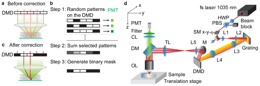
Figure 1: Principle and schematic diagram of two-photon microscopy with Fourier-domain open-channel coupling for scattering correction (2P-FOCUS). (a) The case Without correction. All pixels of the digital micromirror device (DMD) are turned on to pass all incident beams to the objective lens and the scattering sample. These beams are scattered and cannot form a tight focus. (b) The process of generating a correction mask. The first step is to project random intensity patterns, which are orthogonal to each other, onto the DMD and record the corresponding fluorescence intensity using a photomultiplier tube (PMT). The second step is to select the random masks that correspond to high fluorescence intensity and summing these masks to create a grayscale correction mask. The third step is the binarization of the grayscale correction mask for DMD display. (c) The case after correction. By projecting the binary correction mask, only the beams that interfere constructively and generate a bright focus are selected. The illumination power on the sample is maintained at the same level before and after correction by increasing the input power to the DMD to compensate for the power loss due to turning off some pixels. The correction results in a brighter focus compared to the case before correction. (d) Optical schematic diagram of 2P-FOCUS. A femtosecond laser at 1035 nm is used as the light source. A half-wave plate (HWP) and a polarized beam splitter (PBS) are used to control the laser power. A pair of scanning mirrors (SM) is used to scan the focus across the field-of-view. A grating is used to compensate for the spatial dispersion caused by the DMD. L1-L2, L3-L4, and L5-tube lens (TL) are 4-f relay lenses. DMD is located on the conjugate plane of the objective lens’s (OL) back aperture. The objective lens focuses the beams on the sample and collects emitted fluorescence. Fluorescence is detected by a PMT after passing through a dichroic mirror (DM), a collection lens, and a color filter. Sample is mounted on a linear translation stage for collecting z-stack images.

2.1 Principle

2P-FOCUS corrects scattering in three steps: taking measurements, calculating the correction mask, and projecting the correction mask (Fig. 1a-c). First, 2P-FOCUS searches for open channels by projecting random intensity patterns in the Fourier domain while monitoring the fluorescence intensity excited under this frequency modulation (Fig. 1b, step 1). We refer to the ratio between the number of turned-on pixels and the total number of pixels as the sparsity of a random pattern. For example, a random pattern with 0.1 sparsity means that 10% of the pixels are turned on. The pixels on the DMD are binned into $n\times n$ pixel patches, termed “super-pixels”. Random patterns are generated using these super-pixels. Each pattern randomly selects multiple beams that may interfere at a focus after propagating through the unknown scattering media. If these beams interfere constructively, the center lobe of the interference pattern will excite fluorescence through two-photon absorption if the photon density in the center lobe is high enough. Otherwise, the beams do not generate a bright focus, resulting in low or zero fluorescence intensity. Beams that create a bright focus may also be multiply scattered, as long as their phase difference is zero. During our experiments, several thousand measurements are taken in this process. This process is highly nonlinear. The total fluorescence intensity is proportional to the fourth power of the number of interference beams (see Methods for the derivation).

The next step involves calculating the correction mask (Fig. 1b, step 2). The random masks that generate bright fluorescence are selected by thresholding the fluorescence intensity detected by the PMT. Since these beams can create bright center lobes through interference, they have little phase difference. Thus, summing these random patterns generates a new pattern. The multiple beams from this new pattern are coherent and in phase, producing a brighter center lobe. This new pattern serves as the correction mask, selecting beams corresponding to the open channels.

The final step is generating a binary correction mask for DMD projection by thresholding the intensity of the grayscale correction mask (Fig. 1b, step 3). To ensure a fair comparison, we maintain the same illumination power on the sample before and after correction, staying below the thermal damage threshold of biological tissues. For example, if a blank mask is used before correction, allowing no light blockage (Fig. 1a), we then increase the input power to the DMD when applying correction masks to compensate the power blocked by turned-off pixels (Fig. 1c). Power control can also been done by using different thresholds to binarize the grayscale correction mask. Different thresholds result in different illumination power on the sample given the same input power to the DMD, which will be discussed in detail in Section 2.3. As all beams selected by the grayscale correction mask are coherent and in phase, the subset of these beams after binarization remains coherent and in phase. Their interference produces a brighter center lobe compared to the scenario without scattering correction, not only effectively redistributing part of the illumination power from closed to open channels but also increasing the laser power in the center lobe due to coherent interference.

2.2 Experimental setup

The experimental setup is depicted in Fig. 1d and described in the Methods section. We utilized a femtosecond laser with a 1035 nm wavelength for two-photon excitation. Our setup included a near-infrared coated DMD with $1280\times 800$ pixels, of which only the central $800\times 800$ pixels were used, and a pattern rate of 12.5 kHz. Since the DMD is located on the conjugate plane of the back aperture, it induces spatial dispersion in the femtosecond pulses. To correct this spatial dispersion and compress the pulses, we implemented a reflective diffraction grating on the conjugate plane of the DMD [41, 42]. The parameters of the grating, the 4-f relay lenses (L3, L4), and the incident angles were carefully designed and aligned to fully compensate for the spatial dispersion. It’s important to note that the effective groove size of the DMD differs from the micromirror pitch size and was determined empirically. A two-axis scanning mirror system, operating at 1 kHz, is also positioned on the conjugate plane of the DMD. This system scans the focus across the field-of-view and currently represents the speed bottleneck of the system. The scanning mirrors are synchronized with the DMD, allowing the application of different correction patterns to specific sub-regions as necessary. This strategy significantly increases the system’s degrees of freedom, which is the product of the degrees of freedom of both the DMD and the scanning mirrors, thereby effectively controlling a 4D light field [43]. The modulated light field is relayed to the back aperture via 4-f systems and then focused by the objective lens onto the scattering sample. The sample is placed on a linear translation stage for capturing z-stack images. Two-photon excited fluorescence is collected by the objective lens and a collection lens, filtered through a color filter, and detected by a PMT.

2.3 Focusing through bone with 2P-FOCUS

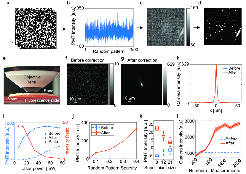
Figure 2: Focusing through bone with 2P-FOCUS. (a) Representative random patterns with a sparsity of 0.4 and a super-pixel radius of 8 pixels. A total of 2,500 such random binary patterns are used for taking measurements of open channels. (b) Fluorescence intensity corresponding to the 2,500 patterns detected by the PMT is shown by the blue line. Random patterns contributing to the top 10% of fluorescence intensity are selected, as indicated by measurements above the red line. (c) The sum of the selected random binary patterns forms the grayscale correction mask. The grayscale intensity indicates the number of patterns contributing to each frequency patch. (d) A binary correction mask is generated by binarizing the grayscale correction mask. (e) Photo of the bone sample and the fluorescence sample. The bone sample is approximately 200-$\mu$m thick at the location where 2P-FOCUS is focused. The fluorescence sample is a microscope slide coated with a thin layer of fluorescent paint. (f) Zoomed-in image of the focus before correction, where no focus is identified. The peak intensity of the image is 10. (g) Zoomed-in image of the focus after correction, showing a clear focus with a peak value of 629. Images (f-g) were taken with a camera that replaced the PMT. (h) Comparison of the intensity profile along the x-axis before (blue line) and after correction (red line). (i) Fluorescence intensity before and after correction, as well as the intensity ratio, as functions of the laser power on the sample. (j) Fluorescence intensity before and after correction as a function of the sparsity of random patterns used for measurements. The radius of super-pixels is 8 pixels. (k) Fluorescence intensity before (blue) and after (red) correction as a function of the size of super-pixels. The sparsity of random patterns is 0.05. Fluorescence intensity before correction is measured with random patterns. (l) Fluorescence intensity before and after correction as a function of the number of measurements. The sparsity of random patterns is 0.01, and the radius of super-pixels is 12 pixels.

We first demonstrate 2P-FOCUS experimentally by focusing through a chicken bone onto a homogeneous fluorescence slide (Fig. 2). We adhered a piece of chicken bone without any exogenous fluorescent labels onto a microscope slide coated with a thin layer of red fluorescent paint (Fig. 2e). The surface of the bone is uneven and the part we focused through is about 200 $\mu$m. The bone is highly scattering and no focus is visible before correction (Fig. 2f) at an illumination power of 7 mW. The mean and standard deviation of intensity of Fig. 2f is $0.58\pm 1.01$. The maximum value of Fig. 2f comes from a hot pixel. In this experiment, We used random patterns with a sparsity of 0.4 and a super-pixel radius of 8 pixels. We will discuss about how sparsity and radius influence the result in the next paragraph. We increased the illumination power on the sample to 76 mW when we took measurements under random illumination, and decreased the illumination power back to 7 mW when we apply the correction mask. We projected 2500 random binary patterns (Fig. 2a) and recorded the corresponding fluorescence intensity (Fig. 2b). We then selected the random patterns corresponding to the top 10% brightest fluorescence (above the red line, Fig. 2b, 250 patterns) and summed them to form the grayscale correction mask (Fig. 2c). The grayscale value of the correction mask indicates the number of patterns that leave the super-pixel open. For instance, the peak value of 159 in Fig. 2c, located on the right bottom side in the Fourier domain, shows that most random patterns (159 out of 250) turned this pixel on to create a bright focus. We then adjusted the half-wave-plate to maximize the power input to the DMD, and binarized the grayscale correction mask (Fig. 2d) using a threshold that ensures the illumination power on the sample remains at 7 mW after modulation by the binary correction mask, which is the same as before correction. In this case, the correction mask only turns on pixles corresponding to ”completely opened” channels (see next paragraph for details). With this correction mask, we achieved a focus with a peak intensity of 629 (Fig. 2g). Figures 2f and 2g, captured by a camera replacing the PMT, display the focus’s image but were not used in the correction process. The bright focus after correction is clearly visible. The distorted shape of the fluorescence spot is due to the scattering of fluorescence as it propagates back through the bone. This occurs because our correction was aimed at maximizing total fluorescence intensity rather than preserving the shape. The intensity profile across the x-axis (Fig. 2h) also demonstrates the significant improvement in fluorescence intensity before and after correction.

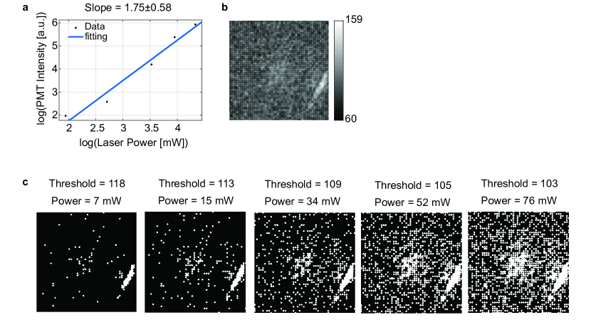
Figure S1: The influence of the binarization threshold on correction masks. (a) Log-log plot of the fluorescence intensity before correction as a function of the laser power on the sample. The slope of the log-log plot is 1.75±0.58, indicating that the fluorescence intensity before correction increases quadratically with the illumination power. (b) The grayscale correction mask, the same as in Fig. 2c. (c) The binary correction masks generated by applying different thresholds to Fig. S1b. These masks are used to produce the data for ”after correction” in Fig. 2i.

We also explore how various factors influence the correction result, including the thresholds for binarization, the sparsity of random patterns, the radius of super-pixels, and the number of measurements. The binarization from Fig. 2c to Fig. 2d depends on the threshold applied to the grayscale correction mask, which controls the illumination power applied to the sample given the same input power to the DMD. The experiment depicted in Fig. 2a-h describes a scenario where the laser power on the sample is 7 mW, corresponding to the first data point in Fig. 2i. The fluorescence intensity value shown in Fig. 2i is measured by the PMT, so it may differ from the values in Figs. f-h. As we increase the illumination power (to 15 mW, 34 mW, 52 mW, and 76 mW), we observe that the fluorescence intensity before correction increases quadratically with the illumination power (see Extended Data Fig. S1a), consistent with the principles of two-photon excitation. Interestingly, the fluorescence intensity after correction, achieved by applying different thresholds to Fig. 2c (see Extended Data Fig. S1b-c), also increases, but does not follow the quadratic rule. This deviation is attributed to the effect of open channel coupling. The brightest pixels in Fig. 2c represent ”completely opened” channels, while other bright pixels indicate ”partially opened” channels. Activating the DMD pixels corresponding to the partially opened channels increases the illumination power on the scattering sample. However, only a portion of this power is delivered to the fluorescence slide and constructively interferes with other beams. The most significant improvement in fluorescence intensity is achieved when the laser power on the sample is low. In other words, the strategy to achieve a large improvement after correction is making the correction mask turn on only the pixels corresponding to ”completely open” channels, while ensuring that the power after modulation is still high enough to achieve a sufficient signal-to-noise ratio. Therefore, in Fig. 2a-h, we chose to maximize the laser power input to the DMD and set a high threshold for binarization in order to couple light into completely open channels and achieve the largest improvement. Fig. 2i clearly demonstrates the presence of open channels in the scattering bone.

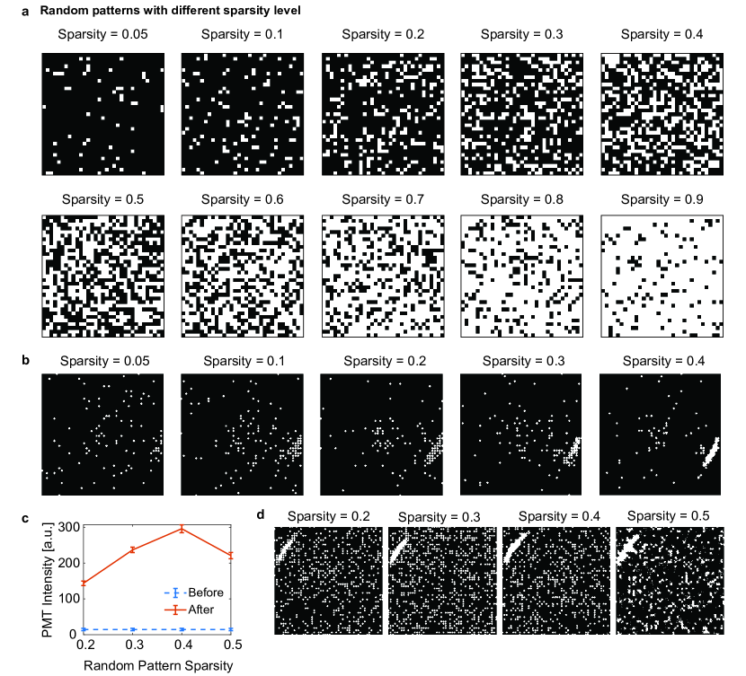
Figure S2: The influence of the sparsity of random patterns on correction masks. (a) Random patterns with varying sparsity levels. Sparsity refers to the percentage of pixels that are turned on out of the total number. When the sparsity is between 0.5 and 0.9, the random patterns act more like notch filters, determining which pixels should be turned off rather than on. (b) Five correction masks used to generate the ’after correction’ data in Fig. 2j. (c) Fluorescence intensity before and after correction as a function of random pattern sparsity. Data were collected from focusing a beam through another region of the bone. The results show that the fluorescence intensity decreases when the correction mask is generated with random patterns having a sparsity of 0.5 compared to those with a sparsity of 0.4. (d) Four correction masks used to generate the ’after correction’ data in Fig. S2b.

The second factor we explore is the sparsity of random patterns, which indicates the percentage of pixels that are turned on out of the total number. For random patterns with a super-pixel radius of 8 pixels, there are 2,500 super pixels in each mask, and a total of 2,500 masks are used, forming a $2500\times 2500$ matrix $P$. For sparsity ranging from 0.05 to 0.9 (see an example in the Extended Data Fig. S2a), these matrices are all orthogonal, as $P^{T}P=I$. The sparsity of random patterns is also related to illumination power. With the same input laser power to the DMD, less sparse patterns block less input power and emit more power to the sample. This increases the signal-to-noise ratio of the raw measurements, consequently improving the accuracy of the correction masks. In the case shown in Fig. 2j, we first measure the fluorescence intensity using random patterns at 7 mW, as in the pre-correction case, and then take raw measurements under different sparsity (0.05, 0.1, 0.2, 0.3, and 0.4), while keeping the input power to the DMD constant. These measurements generate five different correction masks, each with an output power of 7 mW (see Extended Data Fig. S2b). We also took raw measurements under sparsity ranging from 0.2 to 0.5 through another region of the bone and found that the fluorescence signal decreases at the sparsity of 0.5 (see Extended Data Fig. S2c-d). The correction mask derived from the random patterns with 0.4 sparsity shows the most significant improvement in fluorescence intensity in both cases, as depicted in Fig. 2j and Fig.S2c. The random patterns with a sparsity of 0.4, along with the corresponding measurements and the correction mask, are shown in Fig. 2a-d. In practice, the optimal sparsity of random patterns depends on the scattering properties of the sample, and the brightness of the fluorescence signal, and the maximum power of the laser.

We also explored how the radius of super-pixels influences the scattering correction. We used the center square region of the DMD, consisting of $800\times 800=640,000$ pixels. Well-sampling all these pixels requires 640k random patterns, which is too large for the on-chip RAM of the DMD to handle and also requires more computing and experimental time. Therefore, we binned these pixels into super-pixels to accelerate the process. For super-pixels with a radius of $w$, the number of random patterns to well-sample the frequency domain is $800^{2}/(2w+1)^{2}$. We compared the results generated by patterns with $w$ = 8, 12, and 21 (see Fig. 2k). The fluorescence intensity before correction was measured under random pattern modulation with a sparsity of 0.01. The illumination power on the sample was approximately 12 mW, similar before and after correction for all three pattern types. The results indicate that patterns with smaller super-pixels correct scattering more effectively because they identify open channels with greater precision.

We also explored how the number of measurements influences scattering correction. For random patterns with a super-pixel radius of 12 pixels, the minimum number of measurements required for well-sampling is 1024. We generated correction masks with various numbers of raw measurements, ranging from 200 to 2000, and compared the results of the scattering correction. As shown in Fig. 2i, the results improve as the number of measurements increases. However, the improvement becomes trivial with 1024 or more measurements. Considering the computing and experimental time, the results suggest that we should take the minimum number of measurements that adequately sample the Fourier domain, without oversampling.

2.4 Imaging deep in the mouse brain with 2P-FOCUS

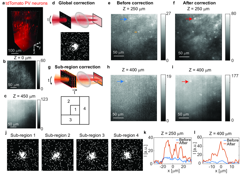
Figure 3: Imaging fluorescence-labeled neurons deep in the mouse brain using 2P-FOCUS. (a) The volumetric view of parvalbumin (PV) interneurons expressing cell-fill tdTomato imaged by 2P-FOCUS in vitro. The image volume is $230\times 230\times 450\mu m^{3}$. (b) The top plane of the image stack shows the dendrites and axons of PV interneurons near the surface of the mouse brain, with no correction applied. (c) The bottom plane of the image stack, 450 $\mu$m deep from (b), shows some cell bodies. Sub-region correction is applied here, and the illumination power is increased compared to (b). The background signal originates from the dendrites and axons of PV interneurons, as cell-fill expression, rather than sparse expression, is used in the experiment. (d) Schematic diagram illustrating global correction and the correction mask used for (e-f). The same mask is used for all scanning locations. The correction mask is generated by optimizing the fluorescence intensity of the reference neuron, indicated by the yellow arrow in (e). (e-f) Images of the same region at 250 $\mu$m depth (e) before and (f) after global correction. Fluorescence intensity is improved by about 3-fold after correction. (g) Schematic diagram for sub-region correction and the sub-regions in (h-i). (h-i) Images of the same region at 400 $\mu$m depth (h) before and (i) after sub-region correction. Fluorescence intensity is improved by about 9.3-fold after correction. (j) The correction masks for four sub-regions used to capture image (i). (k) Comparison of the intensity profile of representative neurons at 250 $\mu$m depth before and after correction (indicated by the blue arrow in (e) and the red arrow in (f)). (l) Comparison of the intensity profile of representative neurons at 400 $\mu$m depth before and after correction (indicated by the blue arrow in (h) and the red arrow in (i)).

2.4.1 Imaging neurons deep in the brain with global and sub-region scattering correction.

We next demonstrate the imaging capabilities of 2P-FOCUS by imaging fluorescence-labeled neurons in the mouse brain. 2P-FOCUS can actively correct scattering during the imaging process with point scanning; that is, it scans the focus across the field-of-view pixel by pixel while applying corresponding correction masks. In our first imaging experiment, we imaged a $230\times 230\times 450\mu m^{3}$ volume in the primary visual cortex of a transgenic mouse brain with cell-fill expression of tdTomato in all parvalbumin (PV) interneurons (see Fig. 3a). The mouse underwent transcardial perfusion with 4% PFA and was then preserved in 4% PFA until imaging. During the imaging session, the whole brain was maintained in phosphate-buffered saline and placed beneath the objective lens. The brain was imaged from the top downward, starting from a plane near the surface. Without any correction, the top plane shows the dendrites and axons of PV interneurons (see Fig. 3b). When imaging the top 250 $\mu$m, we did not apply any correction but gradually increased the illumination power on the sample from 2 mW to 14 mW. The first correction was applied when imaging the plane at a 250 $\mu$m depth (see Fig. 3d-f). Before correction, the image contrast is low, but we can still identify some bright neurons (Fig. 3e). We selected one of the bright neurons near the center of the field-of-view, indicated by the yellow arrow in Fig. 3e, as the reference object. It is important to note that the reference neuron is not a guide star, as it does not need to be a point source; any fluorescent object can be used as a reference. We applied an offset voltage to the scanning mirrors to focus on the reference neuron, and then performed a scattering correction to maximize the fluorescence intensity at this neuron. We used 2,500 random masks with a super-pixel radius of 8 pixels and a sparsity of 0.4 for measurements, and generated a correction mask as shown in the bottom of Fig. 3d. We applied this correction mask to all scanning positions, referring to as a global correction, and acquired the image of the same region after correction (Fig. 3f). The maximum fluorescence intensity is improved by about 3 folds (from 27 to 80). The image contrast is also improved after correction. For example, the three neurons pointed by the arrow (Fig. 3e-f) were not distinguishable before correction but became distinguishable after correction. The intensity profile of the three neurons are plotted in Fig. 3k.

As the imaging depth increases, the global correction mask no longer provides high intensity and high contrast images when the imaging region is larger than the range of the memory effect. We performed corrections at 290 $\mu$m and 380 $\mu$m depths using sub-region correction (see Fig. 3g-j). Sub-region correction involves selecting multiple reference points located in different areas to generate a correction mask for each sub-region, rather than using a single mask for the entire field-of-view. The scanning mirrors are synchronized with the DMD, allowing each sub-region correction mask to be applied when scanning the corresponding regions. Figs. 3h-i show the image at 400 $\mu$m depth before and after sub-region correction. before and after sub-region correction. Four correction masks are generated using reference fluorescent objects located at 380 $\mu$m depth (see Fig. 3g, 3j, and Supplementary Figure X). We initially split the entire field-of-view into 3x3 sub-regions; however, only four out of the nine sub-regions contained bright objects that could serve as references. Therefore, we generated four correction masks, each corresponding to one of these references. We then merged the nearest sub-regions without references into those with references to form four new sub-regions (see Fig. 3g, bottom). We applied these correction masks to the plane at 400 $\mu$m depth, which differs from the correction plane but is within the range of memory effect, and successfully improved both the fluorescence intensity and image contrast (see Fig. 3i) compared to the pre-correction image (Fig. 3h).The intensity profile of a representative neuron, shown in Fig. 3l, indicates that the fluorescence intensity improved by approximately 9.3 times. We noticed that the improvement is less than that achieved when focusing through bone. This is because the fluorescence paint used in the focusing experiment is much brighter than the fluorescence-labeled neurons in the mouse brain. With brighter fluorophores, the correction mask can selectively turn on only the pixels corresponding to completely opened channels and still achieve a sufficient signal-to-noise ratio. In contrast, with less bright fluorophores, the correction mask has to turn on more pixels, including those corresponding to ”partially opened” channels. Therefore, the intensity improvement in brain imaging is less than that in focusing through bone, which is consistent with our result in Fig. 2i. Sub-region correction enables us to image a $230\times 230\mu m$ region deep within the scattering tissue. Therefore, for highly scattering media and large fields-of-view, 2P-FOCUS with sub-region correction can correct scattering outside of an isoplanatic patch, achieving better results than global correction.

2.4.2 Imaging cerebral blood vessels deep in the mouse brain by precise open-channel coupling.

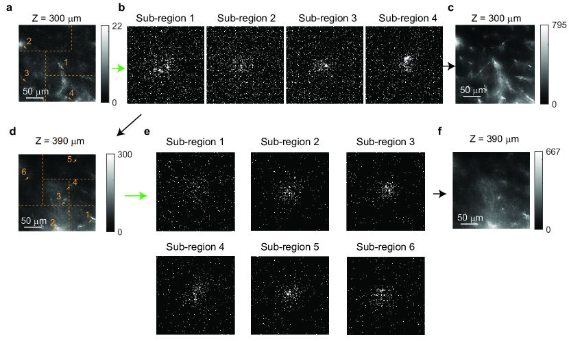
Figure S4: Scattering correction for imaging cerebral vasculatures deep in the mouse brain. The correction is performed with a super-pixel radius of 4 pixels. The green arrows indicate the images used to produce the corresponding masks. The black arrows point at images after correction. The yellow arrows in the images point to fluorescence objects used as references. Note that (a) and (d) are taken with the last correction mask rather than a blank screen on the DMD. (a-c) The sub-region correction is performed at 300 $\mu$m depth. (a) The image before sub-region correction. (b) Four correction masks corresponding to the four sub-regions in (a). The super-pixel radius is 4 pixels. The figure is the same as Fig. 4i. (c) The image after sub-region correction. (d-f) Another sub-region correction is performed at 390 $\mu$m depth. (d) Image taken with the four correction masks in (b), identifying six fractions of blood vessels as references for six sub-regions. (e) Six correction masks corresponding to the six sub-regions. (f) Image after correction.

To further improve the correction and demonstrate the broad applicability of 2P-FOCUS, we imaged another mouse brain in which cerebral blood vessels were labeled through intravascular FITC-dextran injection, using patterns with a super-pixel radius of 4 pixels. Similar to the setup in Fig. 3, the mouse brain was immersed in phosphate-buffered saline and imaged from the top downward. The top plane that we imaged was not on the brain’s surface but below it, as indicated by the visible cross-sections of cerebral blood vessels. We imaged the top 270 $\mu$m volume without correction, meaning all pixels of the DMD were turned on. The maximum intensity projection of the top 100 $\mu$m-thick volume is shown in Fig. 4b, where the cerebral blood vessels are clearly visible. At the bottom of the volume (410 $\mu$m - 510 $\mu$m depth), blood vessels remain visible after scattering correction (see Fig. 4c). Since blood vessels span three-dimensionally, we chose to show the maximum intensity projection rather than a single plane. As the imaging depth increased, we gradually raised the laser power on the sample, from 3 mW (for $Z=0-160\mu m$) to 19 mW (for $Z=250-510\mu m$). We first performed scattering correction at a depth of 270 $\mu$m in three sub-regions, using 2,500 random patterns with a super-pixel radius of 8 pixels in each sub-region. At a depth of 300 $\mu$m, we conducted another sub-region correction with 4 sub-regions, using 8,100 random patterns with a super-pixel radius of 4 pixels in each sub-region (Extended Data Fig. S4a-c). The same 4 correction masks (see Fig. 4h-i) were used when imaging at a depth of 340 $\mu$m (Fig. 4e), revealing fine structures of cerebral capillaries in high contrast (refer to the zoomed-in view in Fig. 4g). Compared to the uncorrected image with the same illumination power (Figs. 4d, 4f), where all pixels on the DMD were turned on, these capillaries were barely visible. We compared the fluorescence intensity of a cross-section of these capillaries in the images before and after correction (Fig. 4j), indicating a 30.6-fold improvement in peak intensity after correction. We also performed another correction at 390 $\mu$m depth with six sub-regions as the imaging depth increases (see Extended Data Fig. S4d-f). Compared to the results in Fig. 3, the outcomes in Fig. 4 show better scattering correction, attributable to the use of patterns with smaller super-pixel radii that generate more precise correction masks. Additionally, the fluorescence labeling of blood vessels is brighter than that of the neurons, despite 1035 nm not being the optimal two-photon excitation wavelength for FITC-dextran. Therefore, the signal-to-noise ratio of measurements under random pattern modulation is higher, resulting in a more accurate correction mask for more precise open-channel coupling. This result demonstrates successful coupling of light into open channels, significantly enhancing laser light propagation through the scattering brain tissue.

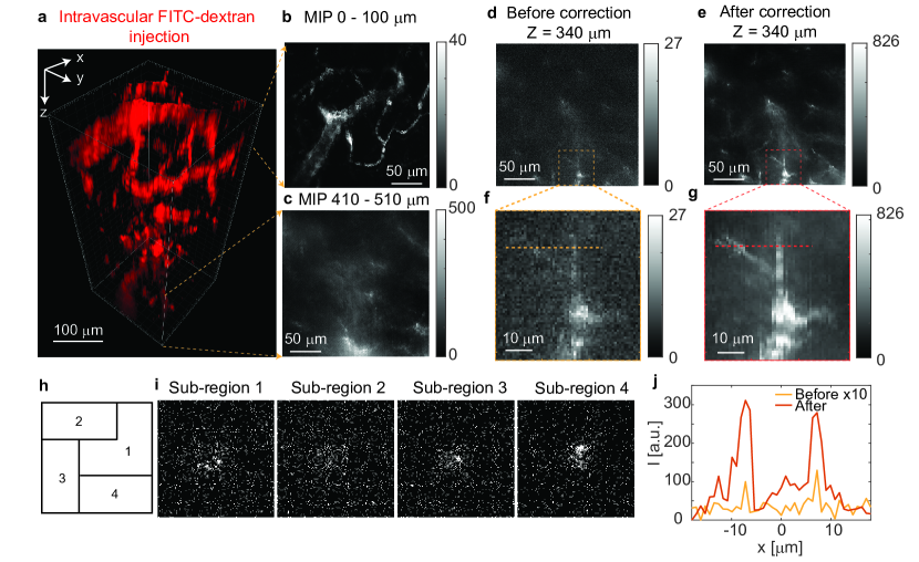
Figure 4: Imaging blood vessels with intravascular fluorophore injection deep in the mouse brain using 2P-FOCUS. (a) Volumetric view of cerebral blood vessels with intravascular FITC-dextran injection, imaged by 2P-FOCUS in vitro. The image volume is $230\times 230\times 510\mu m^{3}$. (b) Maximum intensity projection (MIP) of the top 100 $\mu$m-thick volume along the z axis. (c) MIP of the bottom 100 $\mu$m-thick volume along the z axis. (d) Two-photon image of blood vessels at 340 $\mu$m depth without correction. All pixels of the DMD are turned on. The illumination power on the sample is 19 mW, with a peak fluorescence intensity of 27. (e) Image of the same region as in (d) after sub-region correction. The illumination power on the sample is the same as in (d) at 19 mW, but the peak fluorescence intensity is improved by 30.6-fold, reaching 826. (f-g) Zoomed-in view of the regions in the dashed box in (d-e), showing that small capillaries become visible after scattering correction. (h) The location of the 4 sub-regions on the image plane. (i) The correction masks used in the experiment when acquiring image (e). The radius of super-pixels is 4 pixels and the sparsity is 0.4. (j) Comparison of the fluorescence intensity profile before and after correction along the dashed line in (f-g). The intensity profile of the case before correction is magnified by 10 times for display purposes.

3 Discussion

We have demonstrated that 2P-FOCUS is a novel method for correcting scattering in two-photon microscopy. 2P-FOCUS identifies and couples femtosecond laser light into open channels within scattering tissue by modulating the intensity of light in the Fourier domain, that is, by controlling multiple beam interferences. We demonstrated 2P-FOCUS by focusing through chicken bone, where the focus was initially invisible became distinct after correction. We quantitatively evaluated how various factors affect the correction result, including the number of open channels, the sparsity of random patterns, the super-pixel radius of the patterns, and the number of measurements. We also demonstrated the imaging capability of 2P-FOCUS by capturing image stacks of fluorescence-labeled neurons and cerebral blood vessels in a mouse brain in vitro. The intensity and signal-to-noise ratio of these images were significantly improved compared to images without correction (where all pixels on the DMD were turned on), enabling access to regions over 500 $\mu$m deep in the mouse brain. With sub-region correction, we could correct scattering outside the range of the memory effect, enabling imaging across a $230\times 230\mu m^{2}$ field-of-view deep in the mouse brain. Therefore, 2P-FOCUS can effectively correct scattering and enhance fluorescence signals in a large volume.

2P-FOCUS could be improved in two key aspects. First, to extend the imaging depth further, 2P-FOCUS needs to acquire high signal-to-noise ratio measurements even deep inside the sample. This proves challenging for the current version of 2P-FOCUS, as measurements are taken under completely random modulation in the Fourier domain. This limitation could potentially be overcome by incorporating the correction mask from the plane above to generate the correction mask for the current plane. Second, the current process of generating a correction mask in 2P-FOCUS is not fast enough to correct millisecond-scale dynamic scattering due to blood flow [44]. For instance, collecting 2,500 measurements at a 1 kHz sampling rate takes 2.5 seconds. The computational processes of summation and binarization take about 0.5 seconds, and projecting the correction mask onto the DMD takes 1 millisecond. Consequently, the total time to generate one correction mask is approximately 3 seconds. The speed of this process could be further enhanced with a higher bandwidth data acquisition card, faster scanning mirrors, a higher repetition rate laser, and software designed for auto-correction with closed-loop control.

In summary, 2P-FOCUS is a novel two-photon microscopy system with enhanced scattering control. It can actively boost fluorescence intensity by a few tens of times at the same illumination power on the sample. This capability makes it a powerful tool for deep tissue imaging, facilitating studies in neuroscience, immunology, and cancer.

4 Methods

4.1 2P-FOCUS theory

We describe the process of 2P-FOCUS, which is based on multiple beam interference through scattering media. In the first step, the DMD modulates a collimated laser beam using binary random patterns on a plane relayed to the objective lens’s back aperture. If N super-pixels with a radius of $W$ are turned on, the electric field after intensity modulation is

$$E_{A}(\xi,\eta)=\sum\limits_{i=1}^{N}rect(\frac{\xi-\xi_{i}}{2W})rect(\frac{\eta-\eta_{i}}{2W}).$$ (1)

where $rect$ is the rectangular function describing a turned-on super-pixel. The next step is to calculate the electric field $E_{0}$ on the surface of scattering medium (assuming the uneven of surface is negligible compared to the working distance of objective lens), right before it propagates into the scattering medium. If the thickness of the scattering medium is $\Delta z_{0}$, $E_{0}$ is calculated by

$$E_{0}(x,y)=\mathcal{P}_{-\Delta z_{0}}{\mathcal{F}^{-1}{E_{A}(\xi,\eta)}},$$ (2)

where $\mathcal{F}$ denotes Fourier transform and $\mathcal{P}_{-\Delta z_{0}}$ denotes the linear operator for Fresnel propagation backwards by distance $\Delta z_{0}$:

$$\mathcal{P}_{-\Delta z_{0}}=\mathcal{F}^{-1}{\exp[-j2\pi\Delta z_{0}\sqrt{1/\lambda^{2}-(\xi^{2}+\eta^{2})}]\cdot\mathcal{F}}.$$ (3)

That is, to calculate the incident field on the surface of the sample, we first calculate the electric field at the focus and then back propagate it from the focus to the surface over a distance of $\Delta z_{0}$. Combining Eq. 2 and Eq. 3, the electric field on the surface of the scattering medium can be simplified to

$$E_{0}(x,y)=\mathcal{F}^{-1}{exp[-j2\pi\Delta z_{0}\sqrt{1/\lambda^{2}-(\xi^{2}+\eta^{2})}]\cdot E_{A}(\xi,\eta)}.$$ (4)

In matrix form,

$$E_{0}=F^{-1}diag(H_{\Delta z_{0}}^{*})E_{A},$$ (5)

where $H$ is the forward Fresnel propagation over distance $\Delta z_{0}$. The incident electric field $E_{0}$ propagates in the scattering medium over distance $\Delta z_{0}$, reaching the reference fluorescence object. The excitation field on the fluorescence object is

$$E_{exc}=T_{exc}E_{0},$$ (6)

where $T_{exc}$ is the transmission matrix of the scattering medium. Notice that 2P-FOCUS does not calculate the transmission matrix. The intensity of the excitation field $E_{exc}$ is

$$I_{exc}=|E_{exc}|^{2}$$ (7)

Since fluorescence intensity is quadratically proportional to the intensity of excitation light. Therefore, fluorescence intensity excited by two-photon process is

$$\begin{split}I_{f}&=I_{exc}^{2}\\ &=|T_{exc}F^{-1}diag(H^{*})E_{A}|^{4}.\end{split}$$ (8)

The excited fluorescence propagates backward to exit the scattering medium. Because the wavelength of te fluorescence is different from that of the excitation light, and fluorescence is incoherent (or partial coherent) light while excitation light is coherent light, we use an intensity transmission matrix $T_{f}$ for fluorescence. This matrix is different from the transmission matrix for excitation light, $T_{exc}$. The signal detected by the PMT is the total fluorescence intensity exiting the scattering medium:

$$\begin{split}I&=\sum T_{f}I_{f}\\ &=\sum T_{f}|T_{exc}F^{-1}diag(H^{*})E_{A}|^{4}\\ &=\sum T_{f}|T_{exc}F^{-1}diag(H^{*})\sum\limits_{i=1}^{N}E_{i}|^{4},\end{split}$$ (9)

where $E_{i}$ is the matrix form of binary random pattern with only one super-pixel turned on. According to Eq. 9, computing the correction mask by solving two transmission matrices from a nonlinear equation would be very challenging. On the other hand, the fluorescence intensity is very sensitive to the number of pixels turned on. Probing the correction mask by simultaneously turning on multiple pixels is much more computationally efficient.

4.2 2P-FOCUS Setup

The laser source for 2P-FOCUS is a femtosecond pulsed laser at 1035 nm wavelength and 1 MHz repetition rate (Monaco 1035-40-40 LX, Coherent). The maximum power used for 2P-FOCUS is 2.4 W (The maximum total power of the laser is 40 W but 37.6 W is used to pump an optical parametric amplifier, which is not related to 2P-FOCUS). A polarizing beam splitter cube (PBS123, Thorlabs) and a half-wave-plate (WPHSM05-1310) mounted on a rotation mount (PRM05, Thorlabs) are used to manually adjust the input power to the following optics in the system. A 2-axis galvo-mirror system (GVS002, Thorlabs) are placed on the Fourier plane to scan the laser beam in 2D for imaging in Fig. 3 and Fig. 4. The laser beam is then expended with a 4-f system (L1, LA1401-B, $f_{1}=60mm$, Thorlabs; L2, AC508-100-C-ML, $f_{2}=100mm$, Thorlabs). Next, the laser beam is pre-dispersed by a ruled grating (GR13-0310, 300/mm, 1000 nm blaze, Thorlabs) on the Fourier plane to compensate for the dispersion induced by the DMD. After the grating, the pre-dispersed beam is relayed to the DMD with a 4-f system (L3, LB1199-C, $f_{3}=200mm$, Thorlabs; L4, AC508-200-C-ML, $f_{4}=200mm$, Thorlabs). The DMD (DLP650LNIR, $1280\times 800$ pixels, maximum pattern rate 12.5 kHz, VIALUX) is placed on the Fourier plane to project binary intensity masks. The beam from the DMD is relayed to the back aperture of the objective lens by two 4-f systems, which is simplified as one 4-f system in the optical schematic diagram in Fig. 1d. The first 4-f system is to expend the beam (AC508-150-C-ML, $f=150mm$, and LA1256-C, $f=300mm$). The second 4-f system is to 1:1 relay the beam (two AC508-200-C-ML, $f=200mm$). A dichroic mirror (FF880-SDi01-t3-35x52, Semrock) is used to reflect the beam to the back-aperture of the objective lens (XLUMPlanFL N, 20x, 1.00 NA, water immersion, Olympus). The sample is placed on a manual 3-axis translation stage (MDT616, Thorlabs). In the emission path, a shortpass filter (ET750sp-2p8, CHROMA) is used to block the reflected excitation light. A bandpass filter (AT635/60m, CHROMA) is used in the experiments for Fig. 2 and Fig. 3 for passing through red fluorescence, but removed in the experiments for Fig. 4 because the emission wavelength of FITC-dextran is 520 nm. The fluorescence is detected by a PMT (H15460, Hamamatsu). A sCMOS camera (Kinetix22, Teledyne Photometrics) is used to capture data for Fig. 2f-h, 2i. A beam turning cube (DFM1-E02, Thorlabs) is used to switch between the camera and the PMT. In addition, an one-photon widefield illumination is implemented to locate the sample and find the focal plane before two-photon imaging. The one-photon system consists of a LED (M565L3, Thorlabs), an aspherical condenser lens (ACL25416U-A) to collimate the LED light, and a dichroic mirror (AT600dc, CHROMA) to combine the one-photon path to the two-photon system. A power meter (PowerMax USB - PM10-19C Power, Coherent) is used to measure laser power. During imaging sections, illumination power on the sample is measured on a relayed image plane before the objective lens but after the DMD and multiplied by the power loss rate due to the optical parts between the relayed image plane and the sample.

The 2P-FOCUS system is controlled by a computer (OptiPlex 5000 Tower, Dell) using MATLAB and a data acquisition card (PCIe-6363, X series DAQ, National Instruments) for signal I/O. The voltage signals for external triggering the laser and the DMD, as well as controlling the scanning angles are generated using MATLAB and delivered to the devices by the DAQ card. At the same time, the fluorescence intensity detected by the PMT is read by the DAQ card through an analog input port.

4.3 Data Processing

Process data acquired by the PMT. Data are acquired at 2 MSamples/s for 1 ms per random pattern during scattering correction. Within the 1 ms, the laser is turned on for 0.9 ms and off for 0.1 ms. The raw measurement acquired while the laser is on is subtracted from the raw measurement acquired while the laser is off. After subtraction, all negative voltages are set to zero. Next, a box filter with a width of 3 is applied to the time-lapse signal to remove fluctuations. The final value of the PMT signal under one random pattern modulation is the sum of the processed time-lapse voltage signal acquired over 0.9 ms. Repeating this process for PMT data acquired under all random patterns generates Fig. 2b.

Generate a correction mask from the processed PMT data. The processed PMT data is sorted and the random patterns corresponding to the top 10% brightest data is selected. The sum of the selected random patterns generates Fig. 2c.

Binarize the grayscale correction mask. The intensity distribution on the DMD is measured with a fluorescence slide without scattering media before every experiments, refering to as an intensity map $I_{map}(f_{x},f_{y})$. The intensity map is measured by turning on a super-pixel a time and recording the corresponding fluorescence intensity. The laser power at the image plane $P_{0}$ when all pixels are turned on is also measured. With these two parameters, the laser power $P$ of any intensity mask $I(f_{x},f_{y})$ (a random mask or a correction mask) can be calculated by $P=P_{0}\sum_{f_{x}=1}^{800}\sum_{f_{y}=1}^{800}I(f_{x},f_{y})\cdot I_{map}(f_{x},f_{y})$. We can adjust $P_{0}$ and/or $I(f_{x},f_{y})$ to ensure the laser power on the sample $P$ is the same before and after correction. As we discussed in Section 2.3, the largest improvement is achieved when $P_{0}$ is maximized and $I(f_{x},f_{y})$ is highly selective. In this case, the $P_{0}$ is measured when the input power to the DMD is maximized by turning the half-wave plate. With the known $P_{0}$, $I_{map}$, and $P$, we can calculate the threshold for binarizing the grayscale correction mask accordingly.

Process 2D images An image acquired by the PMT (Fig. 3 and Fig. 4) is generated by reassign the processed PMT data to corresponding scanning locations. The first step is to remove background from the image by subtracting the mean of 300 pixels with the lowest intensity and all negative intensity is set to zero. Next, a $2\times 2$ median filter is applied to the image to remove salt-and-pepper noise. For images acquired by the camera (Fig. 2f-g), we first remove background by subtracting the images with a background image, and then applied a $3\times 3$ median filter to them.

Generate the volumetric view of 3D image stack. Fig. 3a and Fig. 4a were generated using ImarisViewer 10.1.0. The 3D image stacks consist of processed 2D images. The separation between adjacent planes along the z-axis is 10 µm in the original dataset. We interpolated the original image stack 10 times along the z-axis for a better 3D display.

4.4 Sample Preparation

Fluorescence slide with bone. A microscope slide (CAT. NO. 3049, Gold Seal) is coated with a thin layer of fluorescent paint (Tamiya color, fluorescent red). After the paint is dry, a piece of chicken bone is glued on it as the scattering medium.

Whole brain preparation for Fig. 3.The PV tdTomato mouse (PV-IRES-Cre;LSL-tdTomato (Ai9)) was weighed and put into 5% Isoflurane for initial induction. An IP injection of Ketamine hydrochloride 40-80 mg/kg + Xylazine 5-10 mg/kg was given and then the animal was put back into the Isoflurane until the animal’s breathing ceased. The animal was brought to the chemical fume hood and placed in the supine position. An additional amount of isoflurane was placed in a 10 cc syringe with a gauze and placed over the mouse’s nose for additional anesthesia. The hair on the ventral thorax was soaked with 70% alcohol. The anesthetic depth was checked via lack of toe pinch response. A midline incision was made through the skin over the proximal abdomen and thorax. The skin was dissected to expose all underlying muscle. A cut was made into the abdomen, the diaphragm was punctured and a thoracotomy was made by bilateral para- midline incisions through the ribs toward the thoracic inlet, exposing the thoracic viscera. The catheter was placed in the left ventricle, the right atrium was cut to exsanguinate the mouse and allow for drainage of the perfusate. The animal was perfused with cold 4% paraformaldehyde, approximately 12 mls. The brain was dissected from the skull and then placed in cold 4% paraformaldehyde.

Fluorescein isothiocyanate-dextran (FITC-dextran) injection and whole tissue preparation for Fig. 4. Anesthesia was induced in mice with 2.0 -3.0% isoflurane and maintained at 1.5-2.0%. Depth of anesthesia was monitored by toe-pinch and body temperature was maintained by a water perfused thermal pad (Gaymar T/Pump) set at 37^∘C. Fluorescein isothiocyanate-dextran (FITC-dextran) (MW = 2 MDa; Sigma-Aldrich) was injected retro-orbitally at a total volume of 150 $\mu$L. After retro-orbital injection, FITC-dextran was allowed to circulate for a total of 10-15 minutes and the animal was sacrificed. After the animal was sacrificed, the whole brain was collected and stored overnight in PBS at 4^∘C and was imaged the next day.

5 Acknowledgements

We acknowledge the funding support from the Department of Biomedical Engineering at the University of California, Davis (UC Davis). We thank Hillel Adesnik and Janine Beyer at the University of California, Berkeley, for preparing the transgenic mouse brain in Fig. 3 and for providing the PMT used in the microscopy setup. We thank Jiandi Wan and Brianna Urbina at UC Davis for preparing the mouse brain in Fig. 4. We thank Weijian Yang and Zixiao Zhang at UC Davis for helping us measure the pulse width of the laser light before and after dispersion compensation. We thank Peter T. C. So at the Massachusetts Institute of Technology for proofreading the manuscript.

6 Funding

Funding is provided by Dr. Xue’s startup funds from the Department of Biomedical Engineering at the University of California, Davis.

7 Contributions

Y. X. conceived and led the project, and designed and built the microscopy system. Y. X. and Y. L. conducted the experiments and processed the data. D. Z. performed simulations for proof-of-concept using the code provided by Y. X. Y. X. wrote the paper with input from all authors.

8 Ethics declarations

All authors declare no competing interests.

9 Extended Data

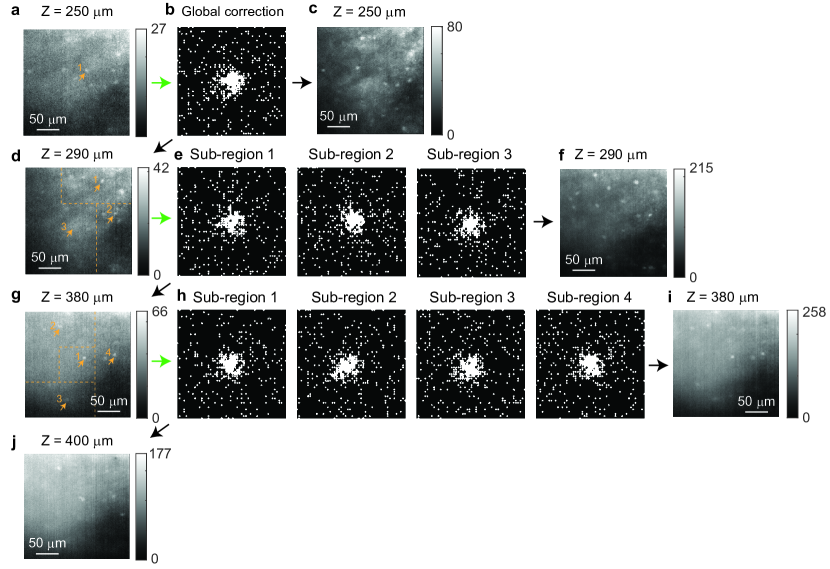
Figure S3: Scattering correction for imaging PV neurons deep in the mouse brain. The green arrows indicate the image is used to produce the corresponding mask. The black arrows point at images after correction. The yellow arrows in the images point to fluorescence objects used as references. Notice that (d), (g), and (j) are taken with last correction mask rather than blank screen on the DMD. (a-c) The first scattering correction is performed at 250 $\mu$m depth. (a) The image before correction, which is the same as Fig. 3e. (b) A single correction mask is produced, which is the same as the bottom plot in Fig. 3d. (c) The image after correction, which is the same as Fig. 3f. (d-f) The second scattering correction is performed at 290 $\mu$m depth. (d) Image taken with the global correction mask in (b). The field-of-view is divided into three sub-regions. Note that we used the background fluorescence as the reference in the sub-region 3 to generate the correction mask. (e) Three correction masks corresponding to the three sub-regions. (f) Image after sub-region correction. (g-i) The third scattering correction is performed at 380 $\mu$m depth. (g) Image taken with the three correction masks in (e). Four neurons are identified as the references for four sub-regions. (h) Four correction masks (identical to Fig. 3j) corresponding to the four sub-regions. (i) Image after correction. (j) Image taken with the four correction masks (identical to Fig. 3i) in (h) at 400 $\mu$m depth.

References

- \bibcommenthead
- Wang et al. [2020] Wang, T., Wu, C., Ouzounov, D.G., Gu, W., Xia, F., Kim, M., Yang, X., Warden, M.R., Xu, C.: Quantitative analysis of 1300-nm three-photon calcium imaging in the mouse brain. Elife 9 (2020)
- Booth [2007] Booth, M.J.: Adaptive optics in microscopy. Philos. Trans. A Math. Phys. Eng. Sci. 365(1861), 2829–2843 (2007)
- Ji [2017] Ji, N.: Adaptive optical fluorescence microscopy. Nat. Methods 14(4), 374–380 (2017)
- Streich et al. [2021] Streich, L., Boffi, J.C., Wang, L., Alhalaseh, K., Barbieri, M., Rehm, R., Deivasigamani, S., Gross, C.T., Agarwal, A., Prevedel, R.: High-resolution structural and functional deep brain imaging using adaptive optics three-photon microscopy. Nat. Methods 18(10), 1253–1258 (2021)
- Rodríguez et al. [2021] Rodríguez, C., Chen, A., Rivera, J.A., Mohr, M.A., Liang, Y., Natan, R.G., Sun, W., Milkie, D.E., Bifano, T.G., Chen, X., Ji, N.: An adaptive optics module for deep tissue multiphoton imaging in vivo. Nat. Methods 18(10), 1259–1264 (2021)
- Gigan et al. [2022] Gigan, S., Katz, O., Aguiar, H.B., Andresen, E.R., Aubry, A., Bertolotti, J., Bossy, E., Bouchet, D., Brake, J., Brasselet, S., Bromberg, Y., Cao, H., Chaigne, T., Cheng, Z., Choi, W., Čižmár, T., Cui, M., Curtis, V.R., Defienne, H., Hofer, M., Horisaki, R., Horstmeyer, R., Ji, N., LaViolette, A.K., Mertz, J., Moser, C., Mosk, A.P., Pégard, N.C., Piestun, R., Popoff, S., Phillips, D.B., Psaltis, D., Rahmani, B., Rigneault, H., Rotter, S., Tian, L., Vellekoop, I.M., Waller, L., Wang, L., Weber, T., Xiao, S., Xu, C., Yamilov, A., Yang, C., Yılmaz, H.: Roadmap on wavefront shaping and deep imaging in complex media. J. Phys. Photonics 4(4), 042501 (2022)
- Yoon et al. [2020] Yoon, S., Kim, M., Jang, M., Choi, Y., Choi, W., Kang, S., Choi, W.: Deep optical imaging within complex scattering media. Nature Reviews Physics 2(3), 141–158 (2020)
- Lee et al. [2022] Lee, H., Yoon, S., Loohuis, P., Hong, J.H., Kang, S., Choi, W.: High-throughput volumetric adaptive optical imaging using compressed time-reversal matrix. Light Sci Appl 11(1), 16 (2022)
- Jeong et al. [2018] Jeong, S., Lee, Y.-R., Choi, W., Kang, S., Hong, J.H., Park, J.-S., Lim, Y.-S., Park, H.-G., Choi, W.: Focusing of light energy inside a scattering medium by controlling the time-gated multiple light scattering. Nat. Photonics 12(5), 277–283 (2018)
- Katz et al. [2012] Katz, O., Small, E., Silberberg, Y.: Looking around corners and through thin turbid layers in real time with scattered incoherent light. Nat. Photonics 6(8), 549–553 (2012)
- Cao et al. [2022] Cao, R., Goumoens, F., Blochet, B., Xu, J., Yang, C.: High-resolution non-line-of-sight imaging employing active focusing. Nat. Photonics 16(6), 462–468 (2022)
- Faccio et al. [2020] Faccio, D., Velten, A., Wetzstein, G.: Non-line-of-sight imaging. Nature Reviews Physics 2(6), 318–327 (2020)
- Tang et al. [2012] Tang, J., Germain, R.N., Cui, M.: Superpenetration optical microscopy by iterative multiphoton adaptive compensation technique. Proc. Natl. Acad. Sci. U. S. A. 109(22), 8434–8439 (2012)
- Papadopoulos et al. [2016] Papadopoulos, I.N., Jouhanneau, J.-S., Poulet, J.F.A., Judkewitz, B.: Scattering compensation by focus scanning holographic aberration probing (F-SHARP). Nat. Photonics 11(2), 116–123 (2016)
- May et al. [2021] May, M.A., Barré, N., Kummer, K.K., Kress, M., Ritsch-Marte, M., Jesacher, A.: Fast holographic scattering compensation for deep tissue biological imaging. Nat. Commun. 12(1), 4340 (2021)
- Kang et al. [2017] Kang, S., Kang, P., Jeong, S., Kwon, Y., Yang, T.D., Hong, J.H., Kim, M., Song, K.-D., Park, J.H., Lee, J.H., Kim, M.J., Kim, K.H., Choi, W.: High-resolution adaptive optical imaging within thick scattering media using closed-loop accumulation of single scattering. Nat. Commun. 8(1), 2157 (2017)
- Yoon et al. [2020] Yoon, S., Lee, H., Hong, J.H., Lim, Y.-S., Choi, W.: Laser scanning reflection-matrix microscopy for aberration-free imaging through intact mouse skull. Nat. Commun. 11(1), 5721 (2020)
- Boniface et al. [2020] Boniface, A., Dong, J., Gigan, S.: Non-invasive focusing and imaging in scattering media with a fluorescence-based transmission matrix. Nat. Commun. 11(1), 6154 (2020)
- Daniel et al. [2019] Daniel, A., Oron, D., Silberberg, Y.: Light focusing through scattering media via linear fluorescence variance maximization, and its application for fluorescence imaging. Opt. Express 27(15), 21778–21786 (2019)
- Xue et al. [2022] Xue, Y., Ren, D., Waller, L.: Three-dimensional bi-functional refractive index and fluorescence microscopy (BRIEF). Biomed. Opt. Express (2022)
- Vellekoop and Mosk [2008] Vellekoop, I.M., Mosk, A.P.: Universal optimal transmission of light through disordered materials. Phys. Rev. Lett. 101(12), 120601 (2008)
- Choi et al. [2011] Choi, W., Mosk, A.P., Park, Q.-H., Choi, W.: Transmission eigenchannels in a disordered medium. Phys. Rev. B Condens. Matter 83(13), 134207 (2011)
- Kim et al. [2012] Kim, M., Choi, Y., Yoon, C., Choi, W., Kim, J., Park, Q.-H., Choi, W.: Maximal energy transport through disordered media with the implementation of transmission eigenchannels. Nat. Photonics 6(9), 581–585 (2012)
- Goetschy and Stone [2013] Goetschy, A., Stone, A.D.: Filtering random matrices: the effect of incomplete channel control in multiple scattering. Phys. Rev. Lett. 111(6), 063901 (2013)
- Davy et al. [2015] Davy, M., Shi, Z., Park, J., Tian, C., Genack, A.Z.: Universal structure of transmission eigenchannels inside opaque media. Nat. Commun. 6, 6893 (2015)
- Ruan et al. [2021] Ruan, H., Xu, J., Yang, C.: Optical information transmission through complex scattering media with optical-channel-based intensity streaming. Nat. Commun. 12(1), 2411 (2021)
- Cao et al. [2022] Cao, J., Yang, Q., Miao, Y., Li, Y., Qiu, S., Zhu, Z., Wang, P., Chen, Z.: Enhance the delivery of light energy ultra-deep into turbid medium by controlling multiple scattering photons to travel in open channels. Light Sci Appl 11(1), 108 (2022)
- Sarma et al. [2016] Sarma, R., Yamilov, A.G., Petrenko, S., Bromberg, Y., Cao, H.: Control of energy density inside a disordered medium by coupling to open or closed channels. Phys. Rev. Lett. 117(8), 086803 (2016)
- Conkey et al. [2012] Conkey, D.B., Caravaca-Aguirre, A.M., Piestun, R.: High-speed scattering medium characterization with application to focusing light through turbid media. Opt. Express, OE 20(2), 1733–1740 (2012)
- Drémeau et al. [2015] Drémeau, A., Liutkus, A., Martina, D., Katz, O., Schülke, C., Krzakala, F., Gigan, S., Daudet, L.: Reference-less measurement of the transmission matrix of a highly scattering material using a DMD and phase retrieval techniques. Opt. Express 23(9), 11898–11911 (2015)
- Wang et al. [2015] Wang, D., Zhou, E.H., Brake, J., Ruan, H., Jang, M., Yang, C.: Focusing through dynamic tissue with millisecond digital optical phase conjugation. Optica 2(8), 728–735 (2015)
- Nam and Park [2020] Nam, K., Park, J.-H.: Increasing the enhancement factor for DMD-based wavefront shaping. Opt. Lett. 45(13), 3381–3384 (2020)
- Zhao et al. [2021] Zhao, T., Ourselin, S., Vercauteren, T., Xia, W.: High-speed photoacoustic-guided wavefront shaping for focusing light in scattering media. Opt. Lett. 46(5), 1165–1168 (2021)
- Yang et al. [2021] Yang, J., He, Q., Liu, L., Qu, Y., Shao, R., Song, B., Zhao, Y.: Anti-scattering light focusing by fast wavefront shaping based on multi-pixel encoded digital-micromirror device. Light Sci Appl 10(1), 149 (2021)
- Zheng et al. [2021] Zheng, C., Park, J.K., Yildirim, M., Boivin, J.R., Xue, Y., Sur, M., So, P.T.C., Wadduwage, D.N.: De-scattering with excitation patterning (DEEP) in temporal focusing microscopy. In: Bio-Optics: Design and Application, pp. 2–6 (2021)
- Wei et al. [2023] Wei, Z., Boivin, J.R., Xue, Y., Burnell, K., Wijethilake, N., Chen, X., So, P.T.C., Nedivi, E., Wadduwage, D.N.: De-scattering deep neural network enables fast imaging of spines through scattering media by temporal focusing microscopy. Res Sq (2023)
- Wijethilake et al. [2023] Wijethilake, N., Anandakumar, M., Zheng, C., So, P.T.C., Yildirim, M., Wadduwage, D.N.: DEEP-squared: deep learning powered de-scattering with excitation patterning. Light Sci Appl 12(1), 228 (2023)
- Xue et al. [2018] Xue, Y., Berry, K.P., Boivin, J.R., Wadduwage, D., Nedivi, E., So, P.T.C.: Scattering reduction by structured light illumination in line-scanning temporal focusing microscopy. Biomed. Opt. Express, BOE 9(11), 5654–5666 (2018)
- Xue et al. [2019] Xue, Y., Boivin, J.R., Wadduwage, D.N., Park, J.K., Nedivi, E., So, P.T.C.: Multiline orthogonal scanning temporal focusing (mosTF) microscopy for scattering reduction in high-speed in vivo brain imaging (2019) arXiv:1905.11540 [physics.optics]
- Escobet-Montalbán et al. [2018] Escobet-Montalbán, A., Spesyvtsev, R., Chen, M., Saber, W.A., Andrews, M., Simon Herrington, C., Mazilu, M., Dholakia, K.: Wide-field multiphoton imaging through scattering media without correction. Sci Adv 4(10), 1338 (2018)
- Geng et al. [2019] Geng, Q., Wang, D., Chen, P., Chen, S.-C.: Ultrafast multi-focus 3-D nano-fabrication based on two-photon polymerization. Nat. Commun. 10(1), 2179 (2019)
- Wang et al. [2020] Wang, Y., Li, H., Hu, Q., Cheng, X., Chen, R., Lv, X., Zeng, S.: Aberration-corrected three-dimensional non-inertial scanning for femtosecond lasers. Opt. Express 28(20), 29904–29917 (2020)
- Xue et al. [2022] Xue, Y., Waller, L., Adesnik, H., Pégard, N.: Three-dimensional multi-site random access photostimulation (3D-MAP). Elife 11, 73266 (2022)
- Qureshi et al. [2017] Qureshi, M.M., Brake, J., Jeon, H.-J., Ruan, H., Liu, Y., Safi, A.M., Eom, T.J., Yang, C., Chung, E.: In vivo study of optical speckle decorrelation time across depths in the mouse brain. Biomed. Opt. Express 8(11), 4855–4864 (2017)