Yadism: Yet Another Deep-Inelastic Scattering Module

Abstract

We present yadism, a library for the evaluation of both polarized and unpolarized deep-inelastic scattering (DIS) structure functions and cross sections up to N³LO in perturbative QCD. The package provides computations of observables in fixed-flavor and zero-mass variable flavor number schemes. The implementation of the general mass variable flavor number schemes is supported through the high virtuality limits for the heavy flavor coefficients. In addition, yadism provides a set of tools for the generation of interpolation grids in the PDF-independent PineAPPL format, allowing to test the PDF dependence on any DIS observable without needing to rerun the computation. This work is part of an ongoing effort to standardize the format of theory predictions in high-energy physics within the pineline framework. The code is open source, written in Python and documented to facilitate usage, integrations, and further extensions. Finally, the code has been benchmarked against the widely used APFEL++ and QCDNUM libraries.

1 Introduction

Deep-inelastic scattering (DIS) experiments provide strong constraints on the structure of hadrons, and around half of the experimental data points, used in the most recent PDF determinations  Hou:2019efy ; Bailey:2020ooq ; NNPDF:2021njg , corresponds to charged current (CC) or neutral current (NC) DIS processes. These include both relatively recent data, such as the ones collected at HERA H1:2009pze ; H1:2018flt , and earlier data such as from the BCDMS Benvenuti:1989rh ; Benvenuti:1989fm experiment. While in recent years the focus of particle physics phenomenology has shifted away from DIS in favor of the description of LHC data, the upcoming Electron-Ion Collider (EIC) projects in the US AbdulKhalek:2021gbh and China Anderle:2021wcy have renewed interest in DIS. Thus, an accurate description of these processes is required to optimally utilize their future data. Reliable predictions for DIS are furthermore relevant for the interpretation of neutrino scattering data Candido:2023utz from neutrino telescopes such as IceCube IceCube:2014stg and experiments such as FASER$\nu$ FASER:2019dxq at the LHC.

In this paper we present yadism, a new software library developed for the calculation of DIS observables with the requirements of the particle physics community of the current age in mind. Yadism differs from other QCD codes such as APFEL Bertone:2013vaa , APFEL++ Bertone:2017gds , HOPPET Salam:2008qg , and QCDNUM Botje:2010ay in various ways, which we briefly highlight in the following.

Yadism includes most of the currently available results in literature, specifically it allows for the computation of polarized Hekhorn:2024tqm and unpolarized structure functions up to next-to-next-to-next-to-leading order (N³LO) N3LO in QCD. Thanks to its modular design, the library can be easily extended as the results of new computations become available. The coefficients, whenever possible, have been benchmarked against APFEL++ and QCDNUM.

Yadism provides both renormalization and factorization scale variations consistently NNPDF:2024dpb and both can be implemented at any order. The currently implemented coefficients allow to perform renormalization scale variations up to N³LO and factorization scale variations up to NNLO. Instead, N³LO factorization scale variations can be included through the EKO evolution code Candido:2022tld .

Yadism can, together with EKO, be used to construct general-mass variable flavor number schemes (GM-VFNS) using coexisting PDFs with different numbers of active flavors. This can avoid nFONLL the perturbative expansion of the evolution kernel as is currently done in the construction of the FONLL scheme Forte:2010ta .

Yadism has a uniform treatment of all heavy quarks, i.e., all features that are available for charm are also available for bottom and top. This strategy opens up the possibility for computations with an intrinsic bottom quark. We provide both the fixed-flavor number scheme (FFNS) and zero-mass variable-flavor number scheme (ZM-VFNS) calculation, as well as the asymptotic limit, $Q^{2}\gg m^{2}$, of the FFNS (FFN0), which is required in the construction of the FONLL scheme Forte:2010ta .

Yadism is interfaced to PineAPPL Carrazza:2020gss ; christopher_schwan_2023_8422248 , a library providing fast-interpolation grids in a unique format and exposing an Application Programming Interface (API) for the programming languages C, C++, Fortran, Rust, and Python making it portable and easy to use. Fast interpolation grids were pioneered by FastNLO Kluge:2006xs and provide a representation of predictions independent of PDFs and the strong coupling, and therefore do not require rerunning the entire toolchain of theory codes if one whishes to assess the impact of the PDF on a theory prediction. This feature can be useful both for PDF fitting and also for the determination of standard model parameters Cridge:2023ztj . The PineAPPL grid output format allows yadism to be integrated into the xFitter framework Alekhin:2014irh ; xFitterDevelopersTeam:2017xal ; xFitter:2022zjb and the pineline framework Barontini:2023vmr . Specifically, the latter consists of various codes with the aim to automate and efficiently compute theory predictions for collider physics processes. Through this toolchain, one can define a collection of consistent theory parameters and observables of interest for which both the partonic coefficients along with the DGLAP evolution kernels (through the EKO package Candido:2022tld ) can conveniently be calculated to produce fast interpolation grids.

Yadism is written in the Python programming language, which is known for its ease of use, and thus reduces the threshold for potential new contributors. For these reasons, development of new functionality can be quick to, e.g., rapidly adopt new computations. Proposed changes to the yadism code are reviewed thoroughly and are subjected to automated checks as part of a Continuous Integration (CI) policy.

So far yadism has already been used in various papers. Specifically, it has been used for the evaluation of neutrino structure functions in Refs. Candido:2023utz ; Cruz-Martinez:2023sdv , and for the computation of polarized structure functions in Ref. Hekhorn:2024tqm . Furthermore, yadism has been adopted by the NNPDF collaboration, who has used it in their most recent papers NNPDF:2024djq ; NNPDF:2024dpb .

The yadism code is open source and free to use under a GPL-3.0 license and can be found in its Github repository:

https://github.com/NNPDF/yadism

along with a user-friendly and up-to-date documentation:

https://yadism.readthedocs.io/en/latest/.

In this paper, we aim to provide an overview of some of the functionalities provided by yadism while we refer the reader to the documentation for an extensive overview of all the available features.

The rest of the paper proceeds as follows: in Section 2, we briefly summarize the theory underlying deep-inelastic scattering and provide details on the yadism implementation. In Section 3, we discuss representative benchmarks in comparison to other available libraries. Finally, we conclude in Section 4 and provide a brief description on possible extensions. In addition, we include two appendices where we briefly comment on the calculation of a new set of formerly unknown coefficient functions in Appendix A and we give an explicit example on how to run yadism in Appendix B.

2 The yadism library

In this section we introduce yadism and provide an overview of its most important features. In the following we assume the standard notation on DIS calculations as can be found, e.g., in any textbook pink-book or in the PDG review Workman:2022ynf .

DIS structure functions can be evaluated within the framework of perturbative Quantum Chromodynamics (pQCD) using collinear factorization Collins:1989gx by convoluting the PDFs with the relevant coefficient functions

$$F\left(x,Q^{2}\right)=\sum_{j}\int_{x}^{1}\frac{dz}{z}C_{j}\left(z,\alpha_{s}\left(Q^{2}\right)\right)f_{j}\left(\frac{x}{z},Q^{2}\right),$$ (1)

where $j$ runs over all possible partons in the initial state, $f_{j}$ denotes the PDF of flavor $j$ and $C_{j}$ are the coefficient function that can be calculated perturbatively as an expansion in the strong coupling $\alpha_{s}$

$$C_{j}\left(z,\alpha_{s}\left(Q^{2}\right)\right)=\sum_{k=0}^{\infty}\left(\frac{\alpha_{s}}{4\pi}\right)^{k}C_{j}^{(k)}(z)\ .$$ (2)

Here and in the following we will assume that the LO coefficient function are of $\mathcal{O}(\alpha_{s}^{0})$ irrespective of the first non-zero order.

All structure functions depend on two kinematic variables: the Bjorken-$x$ and the virtuality $Q^{2}$. Eq. 1 highlights how the DIS structure functions, describing the lepton-hadron interaction, depend on a linear combination of PDFs. Thus, it is clear why DIS processes provide important constraints on flavor separation and are therefore fundamental for the PDFs determination from experimental data.

However, while the factorization formula, Eq. 1, is conceptually simple, if one wishes to actually compute a structure function one needs to define a number of theory parameters and parameters of the experimental setup. Such input settings are passed to yadism through runcards in YAML format, and they are divided into two parts: an observable runcard describing the experimental setup (such as scattering particles, kinematic bins, or helicity settings) and a theory runcard describing the parameters of the theory framework (such as coupling strength, perturbative orders, or quark masses). While observable runcards are usually tailored to a given experiment, theory parameters are usually shared by multiple runs. An example of such runcards is reported in Appendix B, where we show explicitly how to run yadism.

For completeness, the current settings of DIS datasets used in the NNPDF framework are collected in the repository pinecards:

https://github.com/NNPDF/pinecards ,

where we specify the setup for a number of measurements at NMC NewMuon:1996uwk ; NewMuon:1996fwh , SLAC Whitlow:1990gk ; Whitlow:1991uw , BCDMS Benvenuti:1989rh ; Benvenuti:1989fm , CHORUS CHORUS:2005cpn , NuTeV Goncharov:2001qe , EMC Aubert:1982tt , and HERA H1:2009pze ; H1:2018flt . There, we also provide settings for several pseudo-measurements, which are used as theoretical constraints in NNPDF NNPDF:2021njg .

Below, we describe the most important options for the configuration of the observables (Section 2.1) and theories (Section 2.2) that can be defined in the respective runcard. Section 2.3 overviews the partonic coefficient functions implementation and technical details on the computation thereof.

2.1 Observable configuration options

Projectile.

Yadism supports computations of DIS coefficients with massless charged leptons and their associated neutrinos as projectiles in the scattering process. Specifically, to describe, e.g., the HERA data one needs both electrons and positrons and, e.g., for the CHORUS data both neutrinos and anti-neutrinos are needed. Charged leptons can interact both electromagnetically and weakly with the scattered nuclei, whereas neutrinos only carry weak charges. Recently, together with a machine-learning parametrization of experimental data, CC neutrino DIS predictions computed with yadism have been used to extend predictions for neutrino structure functions Candido:2023utz .

Target.

Yadism supports computations with nuclei with mass number $A$ and $Z$ protons as targets in the scattering process. By acting on the coefficients associated to up and down partons yadism implements the isospin symmetry of the form:

$$\begin{pmatrix}c^{\prime}_{u}\\ c^{\prime}_{d}\end{pmatrix}=\frac{1}{A}\begin{pmatrix}Z&A-Z\\ A-Z&Z\end{pmatrix}\begin{pmatrix}c_{u}\\ c_{d}\end{pmatrix}$$ (3)

where $c^{\prime}_{i}$ and $c_{i}$ are the effective and the proton coefficient associated with the parton $i$. This rotation is particularly useful in the context of proton PDF fitting where it can be used to relate neutron, deuteron, and heavier nuclear structure functions to the proton ones. In this way, isospin is used as a first approximation of nuclear correction by just swapping up and down contribution for the amount specified by the target nuclei. In particular for:

  proton targets

($A=1,Z=1$): up and down are kept as they are.

  neutron targets

($A=1,Z=0$): up and down components are fully swapped, such that the up coefficient function is matched to the down PDF and conversely.

  isoscalar targets, i.e. deuteron

($A=2,Z=1$): the effective coefficient functions will be mixed such that $c^{\prime}_{u}$ will be half the original $c_{u}$ and half the original $c_{d}$.

Yadism is completely general with respect to the nuclear target allowing a user to provide values for $A$ and $Z$ as input to the computation. Alternatively, for a number of targets, the name itself can also be provided as input. The readily available targets are: iron ($A=49.618,Z=23.403$), used to describe NuTeV data; lead ($A=208,Z=82$), used to describe CHORUS data; neon and marble ($CaCO_{3}$) with both $A=20,Z=10$, used to describe respectively the BEBCWA59 BEBCWA59:1987rcd and CHARM CHARM:1984ikt data.

Exchanged electroweak gauge boson(s).

DIS can be categorized into three different processes defined by the gauge boson mediating the interaction:

  Electromagnetic current (EM)

corresponds to a process where the exchanged boson is a photon.

  Neutral current (NC)

corresponds to cases where the exchanged boson does not carry any electric charge. Thus, it is a superset of the EM process where also the exchange of the $Z$ boson is allowed. Since for NC two bosons are allowed, interference terms must be included. Because the $Z$ boson has an axial coupling to the incoming lepton it introduces further complications related to $\gamma_{5}$ Gnendiger:2017pys . Note that at small virtualities the $Z$ contributions are suppressed by a factor $Q^{2}/M_{Z}^{2}$.

  Charged current (CC)

corresponds to processes where a $W^{\pm}$ boson is exchanged. The CC process is a flavor-changing current where the CKM-matrix encodes the probabilities to transition between different quark flavors Cabibbo:1963yz ; Kobayashi:1973fv .

Cross sections.

Yadism supports the computation of both structure functions and (reduced) cross sections. In particular, for the unpolarized scattering, we implement the structure functions:

$$F_{2},\ F_{L},\ xF_{3},$$ (4)

and their polarized counter parts:

$$g_{4},\ g_{L},\ 2xg_{1},$$ (5)

where the normalization is chosen such that at LO, all the structure functions are proportional to different PDF combinations of the form $xf(x)$.

While structure functions may only depend on two variables, cross sections may also depend on the inelasticity $y$. Generally, we can write the (reduced) cross sections for a DIS process in terms of the structure functions as

$$\sigma(x,Q^{2},y)=N\left(F_{2}(x,Q^{2})-d_{L}F_{L}(x,Q^{2})+d_{3}xF_{3}(x,Q^{2})\right),$$ (6)

where $N$, $d_{L}$, and $d_{3}$ may depend on the experimental setup or the scattered lepton. The different reduced cross sections implemented in yadism, and their definitions in terms of $N$, $d_{L}$, and $d_{3}$ can be found in the online documentation. The implemented definitions can be used to describe data from HERA, CHORUS, NuTeV, CDHSW Berge:1989hr , and FPF Cruz-Martinez:2023sdv .

Finally, we provide the linearly dependent structure functions:

$$2xF_{1}=F_{2}-F_{L},\quad\quad 2xg_{5}=g_{4}-g_{L}\,.$$ (7)

Flavor tagging.

In general, any total DIS structure function $F$ can be decomposed in three different components, according to the type of quark coupling to the exchanged EW boson:

$$F=F^{(l)}+F^{(h)}+F^{(hl)},$$ (8)

where $F^{(l)}$ denotes the contribution coming from diagrams where all the fermion lines are massless, $F^{(h)}$ is the contribution due to heavy quarks coupling to the EW boson and $F^{(hl)}$ originates from higher order diagrams where a light quark is coupling to the boson, but heavy quarks lines are present.

Given Eq. 8, we support the calculation of fully inclusive (total) observables, where only the lepton is observed in the final state, and flavor tagged final state, where we require a specific heavy quark (charm, bottom, or top) to couple with the mediating boson. This definition coincides with $F^{(h)}$ and it is an infrared-safe definition Forte:2010ta . For example, the charm structure function $F^{(c)}$ can be obtained by assuming the coupling of any quark other than charm and anti-charm to be zero. Instead, a naive definition of $F^{(c)}$ by the heavy final state tag would not be infrared safe. For completeness, also light structure functions $F^{(l)}$ are available, in isolation, although they do not corresponds to any physical observable.

2.2 Theory configuration options

Flavor number schemes.

Flavor number schemes provide a prescription to resolve the ambiguous treatment of heavy quark masses. Generally, to achieve a faithful description of experimental data at scales roughly around the heavy quarks mass $Q\sim m$, quarks should be treated fully massive. However, in the region where $Q\gg m$, quarks should be considered massless. In yadism we allow for 3 different schemes. Only one single heavy quark is allowed at each time.

  Fixed flavor number scheme (FFNS).

The FFNS, is defined as a configuration with a fixed number of flavors at all scales, i.e. all quark masses are fixed to be either light, heavy or decoupled. The FFNS retains all power-like heavy quark corrections $m^{2}/Q^{2}$ and a finite number of logarithmic corrections $\ln(Q^{2}/m^{2})$. This finite number of logarithms, as opposed to a full resummation, limits the perturbative stable region.

  Zero mass-variable flavor number scheme (ZM-VFNS).

In the ZM-VFNS all quark masses in the calculations are either light or decoupled. The number of light quarks $n_{f}$ is not fixed, but instead varies with the number of active flavors depending on the scale of the process, i.e. $n_{f}(Q^{2})$. Specifically, $n_{f}=3$ below $m_{c}$ and this increases as the heavy quark thresholds are crossed, i.e. $Q>m_{h}$, after which the corresponding heavy quark is treated to be light. The ZM-VFNS resums all logarithmic corrections as they are provided by DGLAP evolution. However, the ZM-VFNS does not contain any power-like heavy quark corrections $m^{2}/Q^{2}$ which may be phenomenological important in certain regions of the kinematic phase space.

  Asymtotic fixed flavor number scheme (FFN0).

The FFN0 is similar to the FFNS, but retains only the logarithmic corrections, i.e. it does not contain any power-like heavy quark corrections $m^{2}/Q^{2}$. The FFN0 is constructed as the overlap between FFNS and ZM-VFNS and can be used to construct a GM-VFNS flavor number schemes.

A GM-VFNS can be constructed to overcome the limitation due to potentially large missing corrections of FFNS and ZM-VFNS. One possible scheme is the FONLL scheme Forte:2010ta , which is defined through a linear combination of the FFNS and ZM-VFNS while taking care of possible double counting through the FFN0. A detailed discussion on how to construct the FONLL scheme is given in Ref. nFONLL . Yadism does not provide it explicitly, but all the necessary ingredients FFNS, FFN0, and ZM-VFNS are available.

Renormalization and factorization scale variations.

In perturbative QCD the coefficients $C_{j}$ of Eq. 1, are expanded in powers of $\alpha_{s}$. The estimate of the error introduced by the truncation of such series is quite relevant in multiple precision applications. Some information about the missing higher orders, and the related uncertainty (MHOU), can be extracted from the Callan-Symanzyk equations violation. In this sense, a practical approach to obtain a numerical estimate consists in varying the relevant unphysical scales.

In DIS, the two involved unphysical scales are the renormalization scale, arising from the subtraction of ultraviolet divergences, and the factorization scale, from the subtraction of collinear logarithms in the PDF definition.

The explicit expressions of the $C_{i}$ expansion upon scale variations can be found, e.g., in Sec. 2 of Ref. nnlo-sv-singlet . Generally, these depend, order by order in perturbation theory, on the derivatives of $\alpha_{s}$ and the PDFs with respect to the mentioned scales. The former are the $\beta$-function coefficients and the latter the splitting functions. In yadism, necessary $\beta$-function coefficients are taken from the EKO package, while the $x$-space splitting functions are directly implemented.

At the level of structure function, scale variations can be cast into an additional convolution with a kernel $K$:

$$F(x,\mu\neq Q)=\left(K\otimes C\otimes f\right)(x)$$ (9)

It can be shown that the transformation can be applied a-posteriori to an already computed interpolation grid.

Target mass corrections.

While Eq. 1 is usually derived for the scattering of two massless particles, it is possible to account for the finite mass of the scattering target through target mass corrections tmc-review ; tmc-iranian ; Hekhorn:2024tqm . These corrections become relevant for either small virtualities or large Bjorken-$x$. They can be implemented as an additional convolution and we provide several approximations (corresponding to higher twist expansions) following Ref. tmc-review .

2.3 Implemented partonic coefficients and computation details

Quark mass corrections.

We can differentiate quarks into three different types: light ($m=0$), heavy ($m$ finite) and decoupled ($m=\infty$). Thus, each coefficient function of Eq. 1 can be categorized by the appearance of heavy quark lines in various parts of the diagrams:

  Light

does not contain massive corrections in any part, i.e. all quarks are either light or decoupled.

  Heavy

contains heavy quarks in the output. Note that while some calculation of coefficients with two mass scales are available Ablinger:2018nby , in yadism we currently only provide support for coefficients depending on a single heavy quark mass scale since the impact of the missing corrections are small.

  Intrinsic

contains contributions where the incoming parton is a heavy quark and which thus allows for intrinsic heavy quarks as opposed to radiatively produced heavy quarks.

  Asymptotic

is the $Q\gg m$ limit of either the heavy or intrinsic coefficient. The asymptotic contributions are used in the construction of general mass variable flavor number schemes.

This classification is not exclusive and it is useful to only distinguish coefficient functions but it does not correspond to a unique trivial mapping at the level of structure functions (see Eq. 8). In fact, depending on the chosen variable flavor number scheme, the same coefficients can be reshuffled differently inside each of the components $F^{(l)}$, $F^{(h)}$, and $F^{(hl)}$, or might even not be present at all. For example in the FONLL scheme Forte:2010ta $F^{(c)}$ is computed with massive quarks (using heavy), with massless quarks (using light), and in the asymptotic mass limit (using asymptotic).

Partonic coefficient functions.

NLO $O(a_{s})$	light	heavy	intrinsic	asymptotic
NC	✓vogt-f2nc ; vogt-flnc ; moch-f3nc	✓Hekhorn:2019nlf	✓kretzer-schienbein	✓Buza:1996wv
CC	✓vogt-f2lcc ; vogt-f3cc	✓gluck-ccheavy	✓see Appendix A	✓Buza:1996wv
NNLO $O(a_{s}^{2})$
NC	✓vogt-f2nc ; vogt-flnc ; moch-f3nc	✓Hekhorn:2019nlf	✗	✓Buza:1996wv
CC	✓vogt-f2lcc ; vogt-f3cc	Gao:2017kkx	✗	✓Buza:1996wv
N3LO $O(a_{s}^{3})$
NC	✓vogt-f2nc ; vogt-flnc ; moch-f3nc	✓Kawamura:2012cr ; Laurenti:2024anf ; bbl2023	✗	✓Bierenbaum:2008yu ; Bierenbaum:2009mv ; Ablinger:2010ty ; Ablinger:2014vwa ; Ablinger:2014nga ; Behring:2014eya ; bbl2023
CC	✓vogt-f2lcc ; vogt-f3cc	✗	✗	✗

∗	Available as $K$-factors.

Table 1: Overview of the unpolarized DIS coefficients currently implemented in the yadism library at the corresponding order in perturbative QCD. In the columns we distinguish between light, heavy, intrinsic, and asymptotic. We mark in green coefficient function that are implemented in yadism, in red the ones which are not yet known and in yellow the ones which are not yet implemented in yadism, but available in literature.

Yadism implements both unpolarized and polarized coefficient functions up to N³LO in fixed-order QCD. In Tables 1 and 2 we collect a summary of the coefficient functions as currently implemented. For each perturbative order and process, we distinguish contributions from light, heavy, asymptotic and intrinsic coefficients. In the unpolarized case, Table 1, the light, heavy, and asymptotic contributions are available up to N³LO, except for the CC. The intrinsic components are also available only up to NLO, with the CC part computed very recently, see also Appendix A. The NNLO corrections to CC are known only through $K$-factors Gao:2017kkx and their implementation into yadism is currently work in progress. Instead, for the heavy NC N³LO coefficients, a full analytical result is not known, although approximations can be constructed using information already available through resummations and high virtuality limits Kawamura:2012cr ; Laurenti:2024anf . These coefficient are then implemented together with an uncertainty which can be propagated to the final result.

	light	heavy	intrinsic	asymptotic
NLO $O(a_{s})$	✓Zijlstra:1993sh ; deFlorian:1994wp ; Anselmino:1996cd	✓Hekhorn:2019nlf	✗	✓Buza:1996xr
NNLO $O(a_{s}^{2})$	✓Zijlstra:1993sh ; Borsa:2022irn	✓Hekhorn:2019nlf	✗	✓Buza:1996xr
N3LO $O(a_{s}^{3})$	Blumlein:2022gpp	✗	✗	Behring:2015zaa ; Ablinger:2019etw ; Behring:2021asx ; Blumlein:2021xlc ; Bierenbaum:2022biv ; Ablinger:2023ahe

∗	Only for the $g_{1}$ structure function.

Table 2: Same as Table 1 for NC polarized coefficients.

Similarly, Table 2 provides an overview of the polarized NC coefficient functions currently implemented. As opposed to the unpolarized counterpart, intrinsic polarized coefficient functions are not yet known. At N³LO, only the light coefficient functions for the structure function $g_{1}$ have been computed Blumlein:2022gpp together with the heavy asymptotic limit $Q^{2}\gg m_{h}^{2}$ Behring:2015zaa ; Ablinger:2019etw ; Behring:2021asx ; Blumlein:2021xlc ; Bierenbaum:2022biv ; Ablinger:2023ahe . Their implementation in yadism is left for future updates.

Analytic structure of coefficient functions.

The coefficient functions are not restricted to being regular functions, but they might also correspond to a Dirac delta function or singular distributions. In particular, the latter occur in the light coefficient functions because of massless quarks: whenever the mass of the quark does not prevent IR divergences, it generates plus distributions upon subtractions.

The presence of such distributions does not cause any issue at the analytical level, since the coefficients have to be convoluted with a PDF (or an interpolation polynomial as in Eq. 11), and thus they always act within the scope of an integral. Instead, it does require a dedicated treatment at numerical level, since a distribution cannot be just evaluated (sampled) at given points, and integrated with some approximation, as it is done for regular functions. As common in literature, our $x$-space coefficient function implementation follows the so called regular, singular, local formalism, first described in Floratos:1981hs .

Grid formalism.

It is common for DIS calculations to provide coefficient functions that are directly convoluted with a given PDF, thus returning the predicted value for the requested DIS cross section. This is, however, not necessarily the most practical approach. Instead one may wish to store the computation of the DIS coefficient in an interpolation grid format, thus factorizing the PDF dependence. This is useful in situations where predictions for the same observable have to be computed for different PDFs. The case where this is clearly most relevant is in the context of PDF fits, where at each step of the fitting procedure new comparisons to data are required. In order to unify the treatment inside a PDF fit we follow the pineline framework Barontini:2023vmr and provide interpolation grids, which are more beneficial in a PDF fitting environment.

We introduce an interpolation for the PDF $f(x)$ using the nodes $x_{k}$ and its associated basis of interpolation polynomials $p_{k}(x)$ and write

$$f(x)=\sum_{k}f(x_{k})p_{k}(x)=f^{k}p_{k}(x)$$ (10)

where we defined $f^{k}\equiv f(x_{k})$ and, as usual, sum over repeated indices. While the choice of the nodes is left up to the user, the interpolation basis is fixed to piece-wise Lagrange polynomials, and provided by EKO. The PDF values can then be evaluated directly on the nodes from the original parametrization, or (re-)interpolated from distributed PDF grids (such as provided by LHAPDF Buckley:2014ana ).

To compute an observable $\sigma(x)$ for a given Bjorken-$x$, we can then write

$$\sigma(x)=(C\otimes f)(x)=f^{k}(C\otimes p_{k})(x)=f^{k}C_{k}(x)$$ (11)

and identify $C_{k}(x)=(C\otimes p_{k})(x)$ as the sought-after interpolation grid. Note that in Eq. 11 we suppressed for the sake of readability the flavor dependency, the scale dependency, and the dependency on the strong coupling. In practice, however, we need to keep track of all of them and the PineAPPL format Carrazza:2020gss ; christopher_schwan_2023_8422248 supports such a full breakdown.

3 Benchmarking and Validation

Having described the yadism library and its available features, we will now provide various benchmark analyses. First, we benchmark yadism with some of the most widely used libraries for the computation of DIS observables, namely APFEL++ and QCDNUM. Then we provide representative comparisons on the different prescriptions used to treat heavy quark masses in order to underline their relevance in the different kinematic regions. In all the subsequent comparisons, we adopt a fixed boundary condition defined as a PDF set at a given scale $Q=Q_{0}$. Evolution of the boundary condition, including changing of the number of active flavors, is performed using EKO.

3.1 Benchmarking

Let us start discussing the benchmarks of yadism in comparison to other available libraries for a set of representative structure functions using various flavor number schemes and different perturbative orders. In particular, we show benchmarks for both the unpolarised structure function $F_{2}$ and its polarised counterpart $2xg_{1}$ using ZM-VFNS to highlight the accuracy of the massless calculation. Then we compare $F_{2}^{\text{(c)}}$ with FFNS with $n_{f}=3$ light flavors to highlight heavy quark mass effects. As benchmark tools, we rely on two main programs:

  APFEL++ Bertone:2017gds

which provides DIS observables up to N³LO for massless, unpolarized structure functions and up to NNLO for massless, polarized structure functions. It extends the functionalities of the previous Fortran code APFEL Bertone:2013vaa and has an explicit dependence on the PDF, which can be interfaced via LHAPDF Buckley:2014ana .

  QCDNUM Botje:2010ay

which computes DIS structure functions up to NNLO for unpolarized parton densities and up to NLO for polarized parton densities. The program implements both FFNS and ZM-VFNS and uses polynomial spline interpolation to compute the structure function from a given PDF.

The results reported below show the agreement between yadism and other tools.

Massless coefficient functions.

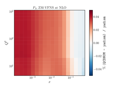
Figure 1: Relative difference between yadism and QCDNUM for the structure function $F_{2}$ using ZM-VFNS as function of $x$ and $Q^{2}$ at NLO (left) and NNLO (right) accuracy.

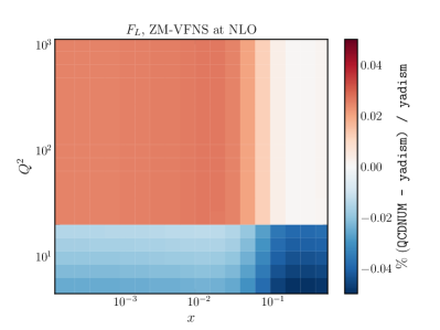
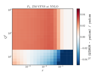
Figure 2: Same as Fig. 1, but now comparing the structure function $F_{L}$.

In the ZM-VFNS only massless coefficient functions are involved, thus we expect to reach good agreement with different tools for a broad range of kinematics. Here we select $x\in[10^{-4},1]$ and $Q^{2}\in[4.0,10^{4}]\,$\mathrm{G}\mathrm{eV}^{2}$$, covering the relevant ranges for DIS phenomenology studies. For simplicity, we focus on NC structure functions, but analogous results hold also for CC DIS. First, in Fig. 1 (Fig. 2) we show the relative difference on $F_{2}$ ($F_{L}$) between yadism and QCDNUM computed at NLO (left) and NNLO (right) accuracy for different kinematics ranges. The overall agreement is within $0.05\text{\,}\mathrm{\char 37\relax}$ with the largest discrepancies visible in the small-$x$ corner.

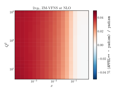
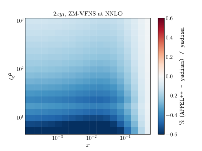
Figure 3: Same as Fig. 1, but now comparing the structure function $2xg_{1}$ computed with yadism and APFEL++.

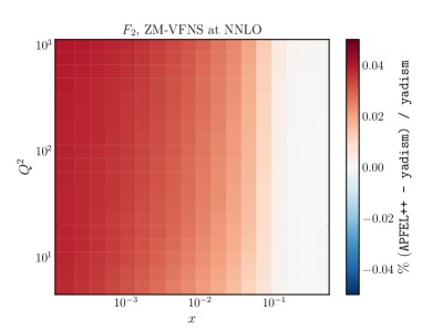
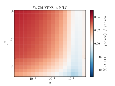
Figure 4: Same as Fig. 1, but now comparing the structure function $F_{2}$ computed with yadism and APFEL++ at NLO (upper left), NNLO (upper right) and N³LO (bottom) accuracy.

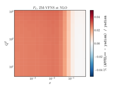
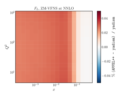
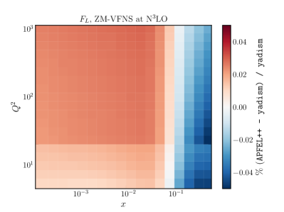
Figure 5: Same as Fig. 4, but now comparing the structure function $F_{L}$.

The analogous comparison with APFEL++ is displayed in Fig. 3 for the polarized structure function $2xg_{1}$ and in Fig. 4 (Fig. 5) again for $F_{2}$ ($F_{L}$) but now at NLO (upper left), NNLO (upper right) and N³LO (bottom) accuracy. Also here the agreement between the different codes is always within $0.05\text{\,}\mathrm{\char 37\relax}$. An exception is found for $2xg_{1}$ at NNLO, where the differences are around $0.5\text{\,}\mathrm{\char 37\relax}$. This larger difference is a result of the different implementation of the nonsinglet (NS) coefficient function – while yadism exploits the exact symmetry of $\Delta C_{1,\mathrm{NS}}^{(2)}=C_{3,\mathrm{NS}}^{(2)}$ Borsa:2022irn , APFEL++ implements the analytical calculation from Zijlstra:1993sh .

From the examples discussed, it is clear that the accuracy of the results does not depend on the perturbative order, i.e. the pattern is not affected by the complexity of the calculation.

Heavy quark mass effects.

Benchmarks of massive calculations are more involved because massive effects are subdominant in most of the kinematic regions, and can be affected by different approximation of the massive coefficient functions Hekhorn:2019nlf ; Beenakker:1988bq .

In order to verify the accuracy of our implementation, we report the comparison for the EM charm-tagged structure function $F^{\text{(c)}}$, computed in FFNS with three light flavors. We adopt the same kinematic range in $Q^{2}$ as in the previous part, but we select $x\in[10^{-4},10^{-1}]$ excluding the large-$x$ region where massive structure functions become small and relative uncertainties large. Moreover, a sufficiently large-$x$ corresponds to an energy that is below the threshold to produce a heavy quark pair ($s<4m^{2}$).

Fig. 6 (Fig. 7) displays the relative difference between APFEL++ and yadism for a NLO and NNLO computations of $F_{2}^{\text{(c)}}$ ($F_{L}^{\text{(c)}}$). In this case, the agreement is around $0.02\text{\,}\mathrm{\char 37\relax}$ at NLO for most of the kinematics and around $0.05\text{\,}\mathrm{\char 37\relax}$ at NNLO.

The analogue comparison to QCDNUM is shown in Fig. 8 at NLO accuracy only demonstrating again a good level of agreement. Here, we cannot perform the comparison at NNLO as QCDNUM does not follow the infrared safe definition of $F^{\text{(c)}}$ (as discussed in Section 2), but instead includes diagrams with a light quark coupling to the boson into their respective $F^{(h)}$ result which start contributing at NNLO.

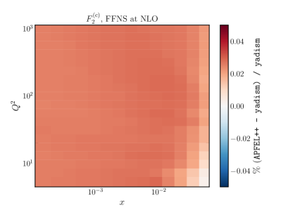
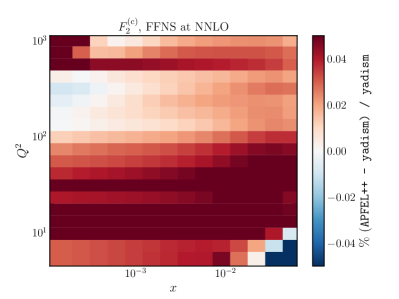
Figure 6: Relative difference between yadism and APFEL++ for the structure function $F_{2}^{\text{(c)}}$ using FFNS, $n_{f}=3$, as function of $x$ and $Q^{2}$ at NLO (left) and NNLO (right) accuracy.

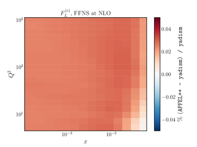
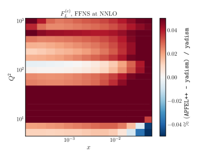
Figure 7: Same as Fig. 6, but now comparing the structure function $F_{L}^{(c)}$.

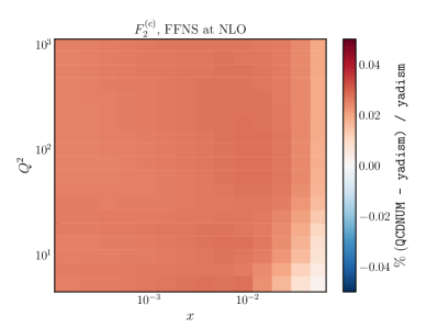
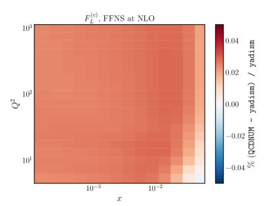
Figure 8: Similar as Fig. 6 and Fig. 7, but now comparing structure function $F_{2}^{(c)}$ (left) and $F_{L}^{(c)}$ (right) computed with yadism and QCDNUM. Note that we can only compare at NLO due to the different conventions adopted by the programs - see text for an explanation.

3.2 Flavour Number Schemes

As discussed in Section 2.2, yadism implements various FNSs with the aim of reducing the impact of missing logarithmic or power-like corrections that become large in certain regions of phase space. In this section we investigate their relevance.

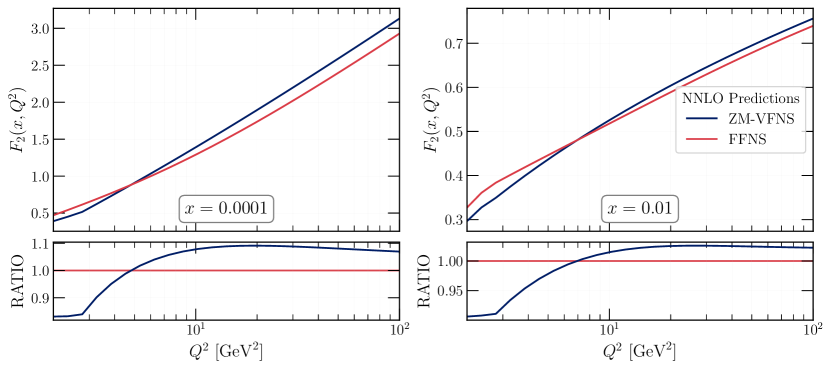
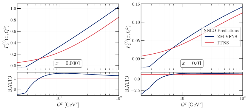
Figure 9: Comparison of the structure functions $F_{2}$ (top) and $F^{(c)}_{2}$ (bottom) using FFNS and ZM-VFNS at NNLO accuracy. The top panels show the absolute comparisons while the bottom ones show the ratio w.r.t. ZM-VFNS.

First, in Fig. 9, we compare the ZM-VFNS and FFNS coefficient functions as a function of $Q^{2}$. Recall that the ZM-VFNS is defined by assuming all (active) quarks to be massless and the FFNS by considering a single heavy quark with a finite mass and the remaining quarks massless. As ZM-VFNS fully resums all (collinear) logarithms $\log(m^{2}/Q^{2})$ we expect both calculations to coincide in the large-$Q^{2}$ region and, indeed, we observe for both structure functions $F_{2}$ and $F_{2}^{(c)}$ a convergence confirming a consistent implementation. However, FFNS is still a fixed order calculation which can eventually only collect a finite number of (collinear) logarithms and hence a finite difference to ZM-VFNS remains.

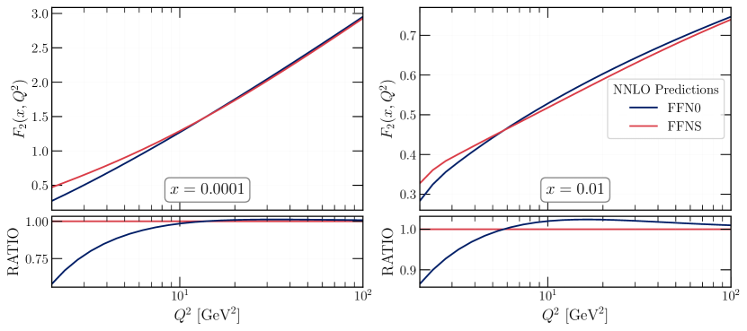
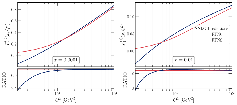
Figure 10: Same as Fig. 9 but now comparing FFNS and FFN0.

Next, in Fig. 10, we compare FFNS and FFN0 coefficient functions as a function of $Q^{2}$. Recall that FFN0 is derived from FFNS by only keeping the finite number of collinear logs and, hence, we expect again both calculations to coincide in the large-$Q^{2}$ region where any power-like mass corrections vanish. While we can indeed observe this convergence at large-$Q^{2}$, we also find a relevant region at mid to low $Q^{2}$ where mass effects can grow up to $25\text{\,}\mathrm{\char 37\relax}$. This latter region can reach up to $O(100)$ times the heavy quark mass and clearly demonstrates the need for GM-VFNSs to improve the accuracy of the prediction.

4 Conclusions and Outlook

In this paper we presented yadism, a new software package to compute cross section and structure functions in deep-inelastic scattering. In Section 2 we reviewed some core features that are relevant in specifying the exact theoretical and experimental setup for which yadism is able to provides calculations. Yadism has been developed with much care to ensure the results are in agreement with the widely used packages QCDNUM and APFEL++ when they should be, and to understand any differences where they do appear. The success of this effort has been shown in the benchmarking exercise presented in Section 3.

While yadism is able to reproduce results also available in QCDNUM and APFEL++, it provides value in following a modular design, allowing it to be easily extended with new coefficient functions, new observables or new DIS-like theories Bissolotti:2023vdw ; McCullough:2022hzr . At the time of writing, yadism has been used for calculations of the photon PDF NNPDF:2024djq , where the photon PDF is computed from DIS cross sections in the LuxQED procedure Manohar:2016nzj ; Manohar:2017eqh ; Bertone:2017bme ; Cridge:2021pxm ; Xie:2023qbn , the study of heavy quark mass effects in polarised DIS scatterings Hekhorn:2024tqm , the study of neutrino-ion interactions at the Forward Physics Facility (FPF) Cruz-Martinez:2023sdv and the determination of low-energy neutrino structure functions Candido:2023utz . Yadism is adopted by the NNPDF collaboration to perform PDF fits where it provides the computations for all fully inclusive DIS measurements by merit of its interface to PineAPPL, and so far this has resulted in the work presented in Refs. NNPDF:2024djq ; NNPDF:2024dpb .

In future it will be possible to adjust the package structure to exploit synergies with a new software package dedicated to the computation of cross sections in semi-inclusive annihilation (SIA). Indeed, DIS and SIA are related by a crossing relation of Feynman diagrams, which makes the mathematical structure of convoluting a collinear distribution, in this case a fragmentation function (FF), with a coefficient function very similar.

Appendix A NLO CC heavy-to-light coefficient functions

In this appendix we sketch the setup used in the computation of NLO heavy-to-light CC coefficient functions. For the NC counterpart, the problem has been solved in kretzer-schienbein . There, the authors study the process

$$Q_{1}(k_{1})+B^{*}(q)\to Q^{\prime}(k_{2})+X$$ (12)

with heavy quarks $Q$ and $Q^{\prime}$ and their respective masses $k_{1}^{2}=m_{1}^{2}$ and $k_{2}^{2}=m_{2}^{2}$ and the scattered boson $B$ with virtuality $Q^{2}=-q^{2}$. Eventually they compute the coefficient functions up to NLO, which agrees with results that were already available (see Ref. (kretzer-schienbein, , Sec. 2.2.1)).

In our case, for CC DIS, this calculation (beyond the LO) cannot be used directly, since we are interested in the scattering

$$Q_{1}(k_{1})+W^{*}(q)\to q^{\prime}(k_{2})+X$$ (13)

now with $k_{2}^{2}=0$. Indeed, in Eq. 12, the explicit dependency on $m_{2}^{2}>0$ shields the calculation from additional infrared singularities, but this does not happen anymore in Eq. 13.

Thus, the CC coefficient functions, with massive initial states, require a dedicated calculation and we report the structure of the obtained results. More details will be discussed in a forthcoming publication Kirill .

In particular, for the intrinsic charm contributions to all three unpolarized structure functions we have:

$$2F_{1}(x,Q^{2}) \supset\int\limits_{x}^{1}\!\frac{d\zeta}{\zeta}C^{1}_{c}(\zeta,\alpha_{s}(Q^{2}),Q^{2}/m_{c}^{2})f_{c}(x/\zeta)$$ (14)

$$\frac{1}{x}F_{2}(x,Q^{2}) \supset\int\limits_{x}^{1}\!\frac{d\zeta}{\zeta}C^{2}_{c}(\zeta,\alpha_{s}(Q^{2}),Q^{2}/m_{c}^{2})f_{c}(x/\zeta)$$ (15)

$$F_{3}(x,Q^{2}) \supset\int\limits_{x}^{1}\!\frac{d\zeta}{\zeta}C^{3}_{c}(\zeta,\alpha_{s}(Q^{2}),Q^{2}/m_{c}^{2})f_{c}(x/\zeta)$$ (16)

where the intrinsic charm PDF $f_{c}(z)$ is now scale independent. The respective coefficient functions are expanded in powers of $\alpha_{s}$ as

$$C^{1}_{c}(\zeta,\alpha_{s}(Q^{2}),Q^{2}/m_{c}^{2}) =e^{2}\left(\delta(1-\zeta)+\frac{\alpha_{s}(Q^{2})C_{F}}{2\pi}C^{1,(1)}_{c}(\zeta,y)\right)$$ (17)

$$C^{2}_{c}(\zeta,\alpha_{s}(Q^{2}),Q^{2}/m_{c}^{2}) =e^{2}\frac{(y-1)}{y}\left(\delta(1-\zeta)+\frac{\alpha_{s}(Q^{2})C_{F}}{2\pi}C^{2,(1)}_{c}(\zeta,y)\right)$$ (18)

$$C^{3}_{c}(\zeta,\alpha_{s}(Q^{2}),Q^{2}/m_{c}^{2}) =e^{2}\left(\delta(1-\zeta)+\frac{\alpha_{s}(Q^{2})C_{F}}{2\pi}C^{3,(1)}_{c}(\zeta,y)\right)$$ (19)

with $C_{F}$ the second Casimir constant of the fundamental color representation and $y=-Q^{2}/m_{c}^{2}$. The lengthy expressions of the actual NLO coefficient functions $C_{c}^{k,(1)}$ are provided as auxillary Mathematica files attached to the arXiv version of this publication. The reader can note the explicit appearance of soft-collinear contributions, which manifest themselves as $\left(\frac{\ln(1-\zeta)}{1-\zeta}\right)_{+}$ and which are not present in kretzer-schienbein .

Appendix B User Manual

The purpose of this appendix is to summarize the steps required to generate an interpolation grid using yadism by providing an explicit example. For more details, we refer to the online documentation containing, among other things, instructions on how to install and use yadism:

https://yadism.readthedocs.io/en/latest/index.html

B.1 Installation

The requirements to run and install yadism are a system with Python3, along with the python package installer pip which enables the installation of packages from the Python Package Index.

With these requirements met, yadism, specifically v0.13.2 discussed in this paper, can be installed by simply running

⬇

1 python -m pip install yadism==0.13.2

B.2 Generating results with yadism

Once yadism is installed, results can be produced by running a single function that takes as input two dictionaries: one with instructions on the observable to be computed, and one containing the theory parameters of the calculation. Once the computation has been run, the output can be saved as a PineAPPL interpolation grid, or convoluted directly to any PDF in LHAPDF format and thereby obtain the requested predictions.

At a first glance, the required number of theory parameters might seems redundant, but this is actually a design choice. In fact, for most of these parameters, yadism does not provide a default value, as we want the user to be fully aware of all the settings entering in the calculation.

The code snippet below provides a simple example of a script that can be used to compute the reduced charm HERA NC cross section.

⬇

1import lhapdf

2import yadism

3from yadbox.export import dump_pineappl_to_file

4

5# OBSERVABLE RUNCARD:

6observablecard = {

7 # Process type: "EM", "NC", "CC"

8 "prDIS": "NC",

9 # Projectile: "electron", "positron", "neutrino", "antineutrino"

10 "ProjectileDIS": "electron",

11 # Scattering target: "proton", "neutron", "isoscalar", "lead", "iron", "neon" or "marble"

12 "TargetDIS": "proton",

13 # Interpolation: if True use log interpolation

14 "interpolation_is_log": True,

15 # Interpolation: polynomial degree, 1 = linear, ...

16 "interpolation_polynomial_degree": 4,

17 # Interpolation: xgrid values

18 # Note: for illustrative purposes the grid is chosen very small here

19 "interpolation_xgrid": [1e-7, 1e-6, 1e-5, 1e-4, 1e-3, 1e-2, 1e-1, 1.0],

20 # Observables configurations

21 "observables": {

22 "XSHERANCAVG_charm": [

23 {

24 "y": 0.8240707777909629,

25 "x": 3e-05,

26 "Q2": 2.5,

27 },

28 {

29 "y": 0.3531731904818413,

30 "x": 7e-05,

31 "Q2": 2.5,

32 },

33 # Add here the kinematics of other datapoints

34 ],

35 # Potentially include observables other than XSHERANCAVG_charm,

36 # each of them has to be: TYPE_heaviness, where heaviness can take:

37 # "charm", "bottom", "top", "total" or "light".

38 },

39 # Projectile polarization faction, float from 0 to 1.

40 "PolarizationDIS": 0.0,

41 # Exchanged boson propagator correction

42 "PropagatorCorrection": 0.0,

43 # Restrict boson coupling to a single parton ? Monte Carlo PID or None for all partons

44 "NCPositivityCharge": None,

45}

46

47# THEORY RUNCARD:

48theorycard = {

49 "CKM": "0.97428 0.22530 0.003470 0.22520 0.97345 0.041000 0.00862 0.04030 0.999152", # CKM matrix elements

50 "FNS": "FFNS", # Flavour Number Scheme, options: "FFNS", "FFN0", "ZM-VFNS"

51 "GF": 1.1663787e-05, # [GeV^-2] Fermi coupling constant

52 "IC": 1, # 0 = perturbative charm only, 1 = intrinsic charm allowed

53 "MP": 0.938, # [GeV] proton mass

54 "MW": 80.398, # [GeV] W boson mass

55 "MZ": 91.1876, # [GeV] Z boson mass

56 "NfFF": 4, # (fixed) number of running flavors, only for FFNS or FFN0 schemes

57 "PTO": 2, # perturbative order in alpha_s: 0 = LO (alpha_s^0), 1 = NLO (alpha_s^1) ...

58 "Q0": 1.65, # [GeV] reference scale for the flavor patch determination

59 "nf0": 4, # number of active flavors at the Q0 reference scale

60 "Qref": 91.2, # [GeV] reference scale for the alphas value

61 "nfref": 5, # number of active flavors at the reference scale Qref

62 "alphas": 0.118, # alphas value at the reference scale

63 "TMC": 1, # include target mass corrections: 0 = disabled, 1 = leading twist, 2 = higher twist approximated, 3 = higher twist exact

64 "XIF": 1.0, # ratio of factorization scale over the hard scattering scale

65 "XIR": 1.0, # ratio of renormalization scale over the hard scattering scale

66 "alphaqed": 0.007496252, # alpha_em value

67 "kcThr": 1.0, # ratio of the charm matching scale over the charm mass

68 "kbThr": 1.0, # ratio of the bottom matching scale over the bottom mass

69 "ktThr": 1.0, # ratio of the top matching scale over the top mass

70 "mc": 1.51, # [GeV] charm mass

71 "mb": 4.92, # [GeV] bottom mass

72 "mt": 172.5, # [GeV] top mass

73 "n3lo_cf_variation": 0, # N3LO coefficient functions variation: -1 = lower bound, 0 = central , 1 = upper bound

74 "QED": 0, # QED correction to running of strong coupling: 0 = disabled, 1 = allowed

75 "MaxNfAs": 5, # maximum number of flavors in running of strong coupling

76 "HQ": "POLE", # heavy quark mass scheme (not yet implemented in yadism)

77 "MaxNfPdf": 5, # maximum number of flavors in running of PDFs (ignored by yadism)

78 "ModEv": "EXA", # evolution solver for PDFs (ignored by yadism)

79}

80

81out = yadism.run_yadism(theorycard, observablecard)

82

83# After running yadism one can either store the result in a pineappl grid

84dump_pineappl_to_file(out,"outputgrid.pineappl.lz4","XSHERANCAVG_charm")

85

86# ... or apply a chosen PDF to compute observable predictions direcly

87pdf = lhapdf.mkPDF("NNPDF40_nnlo_as_01180")

88values = out.apply_pdf(pdf)

lox

References

- (1) T.-J. Hou et al., New CTEQ global analysis of quantum chromodynamics with high-precision data from the LHC, Phys. Rev. D 103 (2021) 014013 [1912.10053].
- (2) S. Bailey, T. Cridge, L.A. Harland-Lang, A.D. Martin and R.S. Thorne, Parton distributions from LHC, HERA, Tevatron and fixed target data: MSHT20 PDFs, Eur. Phys. J. C 81 (2021) 341 [2012.04684].
- (3) NNPDF collaboration, The path to proton structure at 1% accuracy, Eur. Phys. J. C 82 (2022) 428 [2109.02653].
- (4) H1, ZEUS collaboration, Combined Measurement and QCD Analysis of the Inclusive e+- p Scattering Cross Sections at HERA, JHEP 01 (2010) 109 [0911.0884].
- (5) H1, ZEUS collaboration, Combination and QCD analysis of charm and beauty production cross-section measurements in deep inelastic scattering at HERA, Eur. Phys. J. C78 (2018) 473 [1804.01019].
- (6) BCDMS collaboration, A High Statistics Measurement of the Proton Structure Functions and from Deep Inelastic Muon Scattering at High , Phys. Lett. B223 (1989) 485.
- (7) BCDMS collaboration, A High Statistics Measurement of the Deuteron Structure Functions and from Deep Inelastic Muon Scattering at High , Phys. Lett. B237 (1990) 592.
- (8) R. Abdul Khalek et al., Science Requirements and Detector Concepts for the Electron-Ion Collider: EIC Yellow Report, Nucl. Phys. A 1026 (2022) 122447 [2103.05419].
- (9) D.P. Anderle et al., Electron-ion collider in China, Front. Phys. (Beijing) 16 (2021) 64701 [2102.09222].
- (10) A. Candido, A. Garcia, G. Magni, T. Rabemananjara, J. Rojo and R. Stegeman, Neutrino Structure Functions from GeV to EeV Energies, JHEP 05 (2023) 149 [2302.08527].
- (11) IceCube collaboration, Observation of High-Energy Astrophysical Neutrinos in Three Years of IceCube Data, Phys. Rev. Lett. 113 (2014) 101101 [1405.5303].
- (12) FASER collaboration, Detecting and Studying High-Energy Collider Neutrinos with FASER at the LHC, Eur. Phys. J. C 80 (2020) 61 [1908.02310].
- (13) APFEL collaboration, APFEL: A PDF Evolution Library with QED corrections, Comput. Phys. Commun. 185 (2014) 1647 [1310.1394].
- (14) V. Bertone, APFEL++: A new PDF evolution library in C++, PoS DIS2017 (2018) 201 [1708.00911].
- (15) G.P. Salam and J. Rojo, A Higher Order Perturbative Parton Evolution Toolkit (HOPPET), Comput. Phys. Commun. 180 (2009) 120 [0804.3755].
- (16) M. Botje, QCDNUM: Fast QCD Evolution and Convolution, Comput. Phys. Commun. 182 (2011) 490 [1005.1481].
- (17) F. Hekhorn, G. Magni, E.R. Nocera, T.R. Rabemananjara, J. Rojo, A. Schaus et al., Heavy Quarks in Polarised Deep-Inelastic Scattering at the Electron-Ion Collider, 2401.10127.
- (18) NNPDF collaboration, R.D. Ball, A. Barontini, A. Candido, S. Carrazza, J. Cruz-Martinez, L.D. Debbio et al., “The Path to N3LO Parton Distributions.” in preparation, 2024.
- (19) NNPDF collaboration, Determination of the theory uncertainties from missing higher orders on NNLO parton distributions with percent accuracy, 2401.10319.
- (20) A. Candido, F. Hekhorn and G. Magni, EKO: evolution kernel operators, Eur. Phys. J. C 82 (2022) 976 [2202.02338].
- (21) A. Barontini, A. Candido, F. Hekhorn, G. Magni and R. Stegeman, “An FONLL prescription with coexisting flavor number PDFs.” in preparation, 2024.
- (22) S. Forte, E. Laenen, P. Nason and J. Rojo, Heavy quarks in deep-inelastic scattering, Nucl. Phys. B 834 (2010) 116 [1001.2312].
- (23) S. Carrazza, E.R. Nocera, C. Schwan and M. Zaro, PineAPPL: combining EW and QCD corrections for fast evaluation of LHC processes, JHEP 12 (2020) 108 [2008.12789].
- (24) C. Schwan, A. Candido, F. Hekhorn, S. Carrazza and A. Barontini, Nnpdf/pineappl: v0.6.2, Oct., 2023. 10.5281/zenodo.8422248.
- (25) T. Kluge, K. Rabbertz and M. Wobisch, FastNLO: Fast pQCD calculations for PDF fits, in 14th International Workshop on Deep Inelastic Scattering, pp. 483–486, 9, 2006, DOI [hep-ph/0609285].
- (26) T. Cridge and M.A. Lim, Constraining the top-quark mass within the global MSHT PDF fit, Eur. Phys. J. C 83 (2023) 805 [2306.14885].
- (27) S. Alekhin et al., HERAFitter, Eur. Phys. J. C 75 (2015) 304 [1410.4412].
- (28) xFitter Developers’ Team collaboration, xFitter 2.0.0: An Open Source QCD Fit Framework, PoS DIS2017 (2018) 203 [1709.01151].
- (29) xFitter collaboration, xFitter: An Open Source QCD Analysis Framework. A resource and reference document for the Snowmass study, 6, 2022 [2206.12465].
- (30) A. Barontini, A. Candido, J.M. Cruz-Martinez, F. Hekhorn and C. Schwan, Pineline: Industrialization of high-energy theory predictions, Comput. Phys. Commun. 297 (2024) 109061 [2302.12124].
- (31) J.M. Cruz-Martinez, M. Fieg, T. Giani, P. Krack, T. Mäkelä, T. Rabemananjara et al., The LHC as a Neutrino-Ion Collider, 2309.09581.
- (32) NNPDF collaboration, Photons in the proton: implications for the LHC, 2401.08749.
- (33) R. Ellis, W. Stirling and B. Webber, QCD and collider physics, vol. 8, Cambridge University Press (2, 2011).
- (34) Particle Data Group collaboration, Review of Particle Physics, PTEP 2022 (2022) 083C01.
- (35) J.C. Collins, D.E. Soper and G.F. Sterman, Factorization of Hard Processes in QCD, Adv. Ser. Direct. High Energy Phys. 5 (1989) 1 [hep-ph/0409313].
- (36) New Muon collaboration, Accurate measurement of F2(d) / F2(p) and R**d - R**p, Nucl. Phys. B 487 (1997) 3 [hep-ex/9611022].
- (37) New Muon collaboration, Measurement of the proton and deuteron structure functions, F2(p) and F2(d), and of the ratio sigma-L / sigma-T, Nucl. Phys. B 483 (1997) 3 [hep-ph/9610231].
- (38) L.W. Whitlow, S. Rock, A. Bodek, E.M. Riordan and S. Dasu, A Precise extraction of R = sigma-L / sigma-T from a global analysis of the SLAC deep inelastic e p and e d scattering cross-sections, Phys. Lett. B 250 (1990) 193.
- (39) L.W. Whitlow, E.M. Riordan, S. Dasu, S. Rock and A. Bodek, Precise measurements of the proton and deuteron structure functions from a global analysis of the SLAC deep inelastic electron scattering cross-sections, Phys. Lett. B282 (1992) 475.
- (40) CHORUS collaboration, Measurement of nucleon structure functions in neutrino scattering, Phys. Lett. B 632 (2006) 65.
- (41) NuTeV collaboration, Precise measurement of dimuon production cross-sections in Fe and Fe deep inelastic scattering at the Tevatron, Phys. Rev. D64 (2001) 112006 [hep-ex/0102049].
- (42) European Muon collaboration, Production of charmed particles in 250-GeV - iron interactions, Nucl. Phys. B213 (1983) 31.
- (43) BEBC WA59 collaboration, Measurement of the Structure Functions F2 and Xf3 and Comparison With QCD Predictions Including Kinematical and Dynamical Higher Twist Effects, Z. Phys. C 36 (1987) 1.
- (44) CHARM collaboration, Experimental Study of the Nucleon Longitudinal Structure Function in Charged Current Neutrino and Anti-neutrinos Interactions, Phys. Lett. B 141 (1984) 129.
- (45) C. Gnendiger et al., To , or not to : recent developments and comparisons of regularization schemes, Eur. Phys. J. C 77 (2017) 471 [1705.01827].
- (46) N. Cabibbo, Unitary Symmetry and Leptonic Decays, Phys. Rev. Lett. 10 (1963) 531.
- (47) M. Kobayashi and T. Maskawa, CP Violation in the Renormalizable Theory of Weak Interaction, Prog. Theor. Phys. 49 (1973) 652.
- (48) J.P. Berge et al., A Measurement of Differential Cross-Sections and Nucleon Structure Functions in Charged Current Neutrino Interactions on Iron, Z. Phys. C 49 (1991) 187.
- (49) W.L. van Neerven and A. Vogt, NNLO evolution of deep inelastic structure functions: The Singlet case, Nucl. Phys. B 588 (2000) 345 [hep-ph/0006154].
- (50) I. Schienbein et al., A Review of Target Mass Corrections, J. Phys. G 35 (2008) 053101 [0709.1775].
- (51) M. Goharipour and S. Rostami, Implementation of target mass corrections and higher-twist effects in the xFitter framework, Phys. Rev. D 101 (2020) 074015 [2004.03403].
- (52) J. Ablinger, J. Blümlein, A. De Freitas, A. Goedicke, C. Schneider and K. Schönwald, Two-mass three-loop effects in deep-inelastic scattering, PoS LL2018 (2018) 051 [1807.07855].
- (53) J.A.M. Vermaseren, A. Vogt and S. Moch, The Third-order QCD corrections to deep-inelastic scattering by photon exchange, Nucl. Phys. B724 (2005) 3 [hep-ph/0504242].
- (54) S. Moch, J. Vermaseren and A. Vogt, The longitudinal structure function at the third order, Physics Letters B 606 (2005) 123–129 [hep-ph/0411112].
- (55) S. Moch and J. Vermaseren, Deep inelastic structure functions at two loops, Nucl. Phys. B 573 (2000) 853 [hep-ph/9912355].
- (56) F. Hekhorn, Next-to-Leading Order QCD Corrections to Heavy-Flavour Production in Neutral Current DIS, Ph.D. thesis, Tubingen U., Math. Inst., 2019. 1910.01536. 10.15496/publikation-34811.
- (57) S. Kretzer and I. Schienbein, Heavy quark initiated contributions to deep inelastic structure functions, Phys. Rev. D 58 (1998) 094035 [hep-ph/9805233].
- (58) M. Buza, Y. Matiounine, J. Smith and W.L. van Neerven, Charm electroproduction viewed in the variable flavor number scheme versus fixed order perturbation theory, Eur. Phys. J. C 1 (1998) 301 [hep-ph/9612398].
- (59) S. Moch, M. Rogal and A. Vogt, Differences between charged-current coefficient functions, Nucl. Phys. B 790 (2008) 317 [0708.3731].
- (60) S. Moch, J. Vermaseren and A. Vogt, Third-order QCD corrections to the charged-current structure function F(3), Nucl. Phys. B 813 (2009) 220 [0812.4168].
- (61) M. Gluck, S. Kretzer and E. Reya, The Strange sea density and charm production in deep inelastic charged current processes, Phys. Lett. B 380 (1996) 171 [hep-ph/9603304].
- (62) J. Gao, Massive charged-current coefficient functions in deep-inelastic scattering at NNLO and impact on strange-quark distributions, JHEP 02 (2018) 026 [1710.04258].
- (63) H. Kawamura, N.A. Lo Presti, S. Moch and A. Vogt, On the next-to-next-to-leading order QCD corrections to heavy-quark production in deep-inelastic scattering, Nucl. Phys. B 864 (2012) 399 [1205.5727].
- (64) N. Laurenti, Construction of a next-to-next-to-next-to-leading order approximation for heavy flavour production in deep inelastic scattering with quark masses, 2401.12139.
- (65) A. Barontini, M. Bonvini and N. Laurenti, Implementation of DIS at N3LO for PDF determinations, in preparation (2024) .
- (66) I. Bierenbaum, J. Blumlein, S. Klein and C. Schneider, Two-Loop Massive Operator Matrix Elements for Unpolarized Heavy Flavor Production to O(epsilon), Nucl. Phys. B 803 (2008) 1 [0803.0273].
- (67) I. Bierenbaum, J. Blümlein and S. Klein, Mellin Moments of the Heavy Flavor Contributions to unpolarized Deep-Inelastic Scattering at and Anomalous Dimensions, Nucl. Phys. B 820 (2009) 417 [0904.3563].
- (68) J. Ablinger, J. Blümlein, S. Klein, C. Schneider and F. Wissbrock, The Massive Operator Matrix Elements of for the Structure Function and Transversity, Nucl. Phys. B 844 (2011) 26 [1008.3347].
- (69) J. Ablinger, A. Behring, J. Blümlein, A. De Freitas, A. Hasselhuhn, A. von Manteuffel et al., The 3-Loop Non-Singlet Heavy Flavor Contributions and Anomalous Dimensions for the Structure Function and Transversity, Nucl. Phys. B 886 (2014) 733 [1406.4654].
- (70) J. Ablinger, A. Behring, J. Blümlein, A. De Freitas, A. von Manteuffel et al., The 3-Loop Pure Singlet Heavy Flavor Contributions to the Structure Function and the Anomalous Dimension, 1409.1135.
- (71) A. Behring, I. Bierenbaum, J. Blümlein, A. De Freitas, S. Klein and F. Wißbrock, The logarithmic contributions to the asymptotic massive Wilson coefficients and operator matrix elements in deeply inelastic scattering, Eur. Phys. J. C 74 (2014) 3033 [1403.6356].
- (72) E.B. Zijlstra and W.L. van Neerven, Order- corrections to the polarized structure function , Nucl. Phys. B 417 (1994) 61.
- (73) D. de Florian and R. Sassot, O (alpha-s) spin dependent weak structure functions, Phys. Rev. D 51 (1995) 6052 [hep-ph/9412255].
- (74) M. Anselmino, P. Gambino and J. Kalinowski, New proton polarized structure functions in charged current processes at HERA, Phys. Rev. D 55 (1997) 5841 [hep-ph/9607427].
- (75) M. Buza, Y. Matiounine, J. Smith and W.L. van Neerven, O (alpha-s**2) corrections to polarized heavy flavor production at Q**2 is m**2, Nucl. Phys. B 485 (1997) 420 [hep-ph/9608342].
- (76) I. Borsa, D. de Florian and I. Pedron, The full set of polarized deep inelastic scattering structure functions at NNLO accuracy, Eur. Phys. J. C 82 (2022) 1167 [2210.12014].
- (77) J. Blümlein, P. Marquard, C. Schneider and K. Schönwald, The massless three-loop Wilson coefficients for the deep-inelastic structure functions F2, FL, xF3 and g1, JHEP 11 (2022) 156 [2208.14325].
- (78) A. Behring, J. Blümlein, A. De Freitas, A. von Manteuffel and C. Schneider, The 3-Loop Non-Singlet Heavy Flavor Contributions to the Structure Function at Large Momentum Transfer, Nucl. Phys. B 897 (2015) 612 [1504.08217].
- (79) J. Ablinger, A. Behring, J. Blümlein, A. De Freitas, A. von Manteuffel, C. Schneider et al., The three-loop single mass polarized pure singlet operator matrix element, Nucl. Phys. B 953 (2020) 114945 [1912.02536].
- (80) A. Behring, J. Blümlein, A. De Freitas, A. von Manteuffel, K. Schönwald and C. Schneider, The polarized transition matrix element of the variable flavor number scheme at , Nucl. Phys. B 964 (2021) 115331 [2101.05733].
- (81) J. Blümlein, A. De Freitas, M. Saragnese, C. Schneider and K. Schönwald, Logarithmic contributions to the polarized O(s3) asymptotic massive Wilson coefficients and operator matrix elements in deeply inelastic scattering, Phys. Rev. D 104 (2021) 034030 [2105.09572].
- (82) I. Bierenbaum, J. Blümlein, A. De Freitas, A. Goedicke, S. Klein and K. Schönwald, polarized heavy flavor corrections to deep-inelastic scattering at , Nucl. Phys. B 988 (2023) 116114 [2211.15337].
- (83) J. Ablinger, A. Behring, J. Blümlein, A. De Freitas, A. von Manteuffel, C. Schneider et al., The first-order factorizable contributions to the three-loop massive operator matrix elements and , 2311.00644.
- (84) E.G. Floratos, C. Kounnas and R. Lacaze, Higher Order QCD Effects in Inclusive Annihilation and Deep Inelastic Scattering, Nucl. Phys. B 192 (1981) 417.
- (85) A. Buckley, J. Ferrando, S. Lloyd, K. Nordstr¨om, B. Page, M. Rüfenacht et al., LHAPDF6: parton density access in the LHC precision era, Eur. Phys. J. C 75 (2015) 132 [1412.7420].
- (86) W. Beenakker, H. Kuijf, W.L. van Neerven and J. Smith, QCD Corrections to Heavy Quark Production in p anti-p Collisions, Phys. Rev. D 40 (1989) 54.
- (87) C. Bissolotti, R. Boughezal and K. Simsek, SMEFT probes in future precision DIS experiments, Phys. Rev. D 108 (2023) 075007 [2306.05564].
- (88) M. McCullough, J. Moore and M. Ubiali, The dark side of the proton, JHEP 08 (2022) 019 [2203.12628].
- (89) A. Manohar, P. Nason, G.P. Salam and G. Zanderighi, How bright is the proton? A precise determination of the photon parton distribution function, Phys. Rev. Lett. 117 (2016) 242002 [1607.04266].
- (90) A.V. Manohar, P. Nason, G.P. Salam and G. Zanderighi, The Photon Content of the Proton, JHEP 12 (2017) 046 [1708.01256].
- (91) NNPDF collaboration, Illuminating the photon content of the proton within a global PDF analysis, SciPost Phys. 5 (2018) 008 [1712.07053].
- (92) T. Cridge, L.A. Harland-Lang, A.D. Martin and R.S. Thorne, QED parton distribution functions in the MSHT20 fit, Eur. Phys. J. C 82 (2022) 90 [2111.05357].
- (93) K. Xie, B. Zhou and T.J. Hobbs, The Photon Content of the Neutron, 2305.10497.
- (94) K. Kudashkin. in preparation, 2024.
lox