Strong-Field Ionization Phenomena Revealed by Quantum Trajectories

Abstract

The photoionization dynamics of atoms in intense and ultrashort laser pulses is explored using quantum trajectories. This approach is shown to provide a comprehensive and consistent framework to investigate ultra-fast phenomena in atoms interacting with laser fields. In particular, we introduce novel parameters that reveal crucial aspects of the electron dynamics in a time-dependent potential barrier and indicate the transition between different ionization regimes. These quantities offer additional perspectives to access information on the complex ionization mechanisms in strong fields.

Recent progress in generating bright and ultrashort laser pulses Paul et al. (2001); Li et al. (2020); Maroju et al. (2020); Zhang et al. (2017) has profoundly transformed our approach to light-matter interaction. In particular, these advances have opened the way to observe and manipulate the electron dynamics in atoms and molecules at their intrinsic temporal scale Stewart et al. (2023); Isinger et al. (2017); Sainadh et al. (2019). In spite of these remarkable strides, the theoretical modeling of strong-field phenomena, which is pivotal for the advancement of attosecond science, remains challenging. One major difficulty arises from the complexity in describing and comprehending the electron dynamics under the combined influence of the Coulomb interaction between charged particles and an intense electromagnetic field Popruzhenko (2014); Faisal (1973); Reiss (1980); Agostini and DiMauro (2012); Smirnova et al. (2008); Torlina and Smirnova (2012).

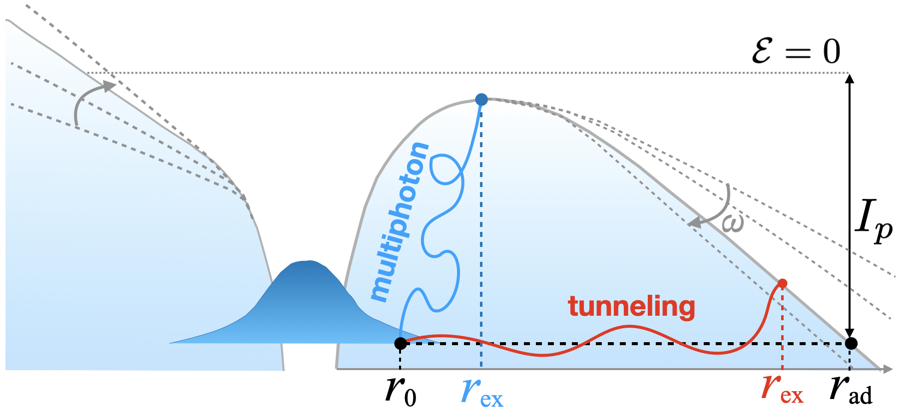
Figure 1: Schematic illustration of multiphoton (vertical channel) and tunneling (horizontal channel) ionization. See text for the definition of the various parameters.

When an atom is subjected to the oscillating electric field of a laser beam, its electronic wave function is perturbed by the time-varying potential barrier. If sufficient energy is transferred to the atom, this process eventually leads to the emission of one or many electrons (photoelectric effect). One usually distinguishes two main types of photoionization mechanisms, as illustrated in Fig. 1. In the vertical channel, referred to as multiphoton ionization Delone and Krainov (2000); Ivanov et al. (2005), the barrier oscillates rapidly compared to the characteristic response time of the system, such that the electron experiences periodic “heating” due to the swift changes of the potential. As a result, the electron accumulates an average energy during each pulse cycle, gradually drifting away from the ionic core until it becomes free to escape. This regime of ionization is chaotic Ivanov et al. (2005) and dominates for weak and high-frequency fields. Conversely, in the horizontal channel, known as tunneling ionization, the wave function has sufficient time to adjust to the gradual changes in the potential, allowing its tail to “leak” via tunneling through the quasi-static barrier. For slow-moving barriers, this regime becomes adiabatic and the electron energy under the barrier does not vary significantly before the electron escapes the barrier. In general, however, the multiphoton and tunneling ionization regimes coexist, i.e., an electron can always gain energy nonadiabatically inside a moving barrier.

The Keldysh parameter, $\gamma_{\rm\footnotesize\textsc{k}}\equiv\omega\sqrt{2I_{p}}/E_{0}$ Keldysh (1965), provides a quantitative understanding of the dominant photoionization mechanism by comparing the period of the oscillating electric field $T$ to the characteristic response time $\tau$ of the system. By taking $\tau$ as the tunneling time of the electron from the inner to the outer classical turning points, a transparent expression for the Keldysh parameter is obtained Topcu and Robicheaux (2012); Keldysh (1965); Delone and Krainov (1998); Ivanov et al. (2005), depending only on the light’s angular frequency $\omega$, the maximum field strength $E_{0}$, and the ionization potential $I_{p}$ of the atom. The multiphoton picture is privileged when $\gamma_{\rm\footnotesize\textsc{k}}\gg 1$, whereas the tunneling mechanism dominates for $\gamma_{\rm\footnotesize\textsc{k}}\leq 1$.

While the Keldysh parameter provides a simple analytical formula revealing the dominant photoionization mechanism, it also has severe limitations Reiss (2010); Popruzhenko (2014); Topcu and Robicheaux (2012). For instance, it disregards the nature of the binding potential and the role of excited states Trombetta et al. (1989); Mishima et al. (2002). Moreover, $\gamma_{\rm\footnotesize\textsc{k}}$ only considers the pulse at its maximum strength and does not account for the details of the pulse, such as its duration, envelope, and carrier-envelope phase (CEP), despite their known critical roles in strong fields Chetty et al. (2022); Karamatskou et al. (2013). It also wrongly assumes that the tunnelling wave packet always starts from the classically allowed region Douguet and Bartschat (2018), while the possibility for over-the-barrier ionization (OBI) Krainov (1995); Schuricke et al. (2011) (i.e., when the top of the barrier gets below the initial electronic state energy) is neglected. Despite theoretical improvements Arbó et al. (2008); Popruzhenko et al. (2008); Smirnova et al. (2008); Torlina and Smirnova (2012); Topcu and Robicheaux (2012); Wang et al. (2019); Zheltikov (2016); Mishima et al. (2002), there remains a critical need for quantitative approaches unraveling the electron dynamics in strong fields Popruzhenko (2014).

On the other hand, the dynamics of an electron exiting a potential barrier becomes rapidly classical Heldt et al. (2023); Xie et al. (2022); Ni et al. (2016), thus enabling an alternative description via trajectory-based methods Camus et al. (2017); Salières et al. (2001); Yang and Robicheaux (2016); Tan et al. (2021). These approaches, extensively used in strong-field physics, offer an appealing avenue to bridge quantum and classical ideas Xie et al. (2022); Ni et al. (2016). Notably, they form the cornerstone of the three-step model Krause et al. (1992); Corkum (1993); Corkum and Krausz (2007) and can be integrated in more sophisticated methodologies, e.g., analytic tunneling rates with imaginary time methods Perelomov et al. (1966) or Wigner phase-space distributions Hack et al. (2021) to improve the treatment of strong-field phenomena.

In this Letter, we employ de Broglie-Bohm quantum trajectories Dürr and Teufel (2009); Botheron and Pons (2010); Benseny et al. (2014); Jooya et al. (2015); Zimmermann et al. (2016) as a methodology to establish a comprehensive and consistent framework covering both the short-range region, dominated by quantum phenomena, and the large-distance region where electron trajectories exhibit classical behavior. This approach enables the introduction of a quantum-trajectory adiabatic parameter, which extends the application of the Keldysh parameter by offering more intricate and sensitive insights into the photoionization mechanism. Moreover, this framework enables the quantification of the degree of OBI and, more broadly, has the potential to unveil additional aspects of strong-field physics by extracting the complex information encoded in a time-dependent wave function.

Our approach to compute quantum trajectories starts with solving the time-dependent Schrödinger equation (TDSE) Douguet et al. (2016), $i\hbar\partial_{t}|\Psi\rangle=\hat{H}(t)|\Psi\rangle$, in the single-active electron (SAE) picture. [Unless stated otherwise, atomic units (a.u.) are used throughout this manuscript.] In the Coulomb gauge and dipole approximation, $\hat{H}(t)=\hat{H}_{0}+\hat{H}_{\rm int}(t)$, where $\hat{H}_{0}=\hat{T}+\hat{V}$ is the field-free hamiltonian, $\hat{T}$ and $\hat{V}$ are the kinetic and potential energies, respectively, and $\hat{H}_{\rm int}=-\bm{p}\cdot{\bm{A}}(t)$ is the light-atom interaction in the velocity gauge. The vector potential, ${\bm{A}}(t)=-A_{0}F(t)\sin{(\omega t})\,\hat{{\bm{x}}}$, has a period $T$, is linearly polarized along the $x$ axis, has an amplitude $A_{0}$, and an envelope $F(t)=\cos^{4}(\pi t/NT)$ for $N$ cycles with $t\in[-NT/2,NT/2]$. The electric field, ${\bm{E}}(t)=-d{\bm{A}}(t)/dt$, reaches its maximum strength $E_{0}$, corresponding to an intensity $I=E_{0}^{2}/2$, near the envelope maximum at $t=0$.

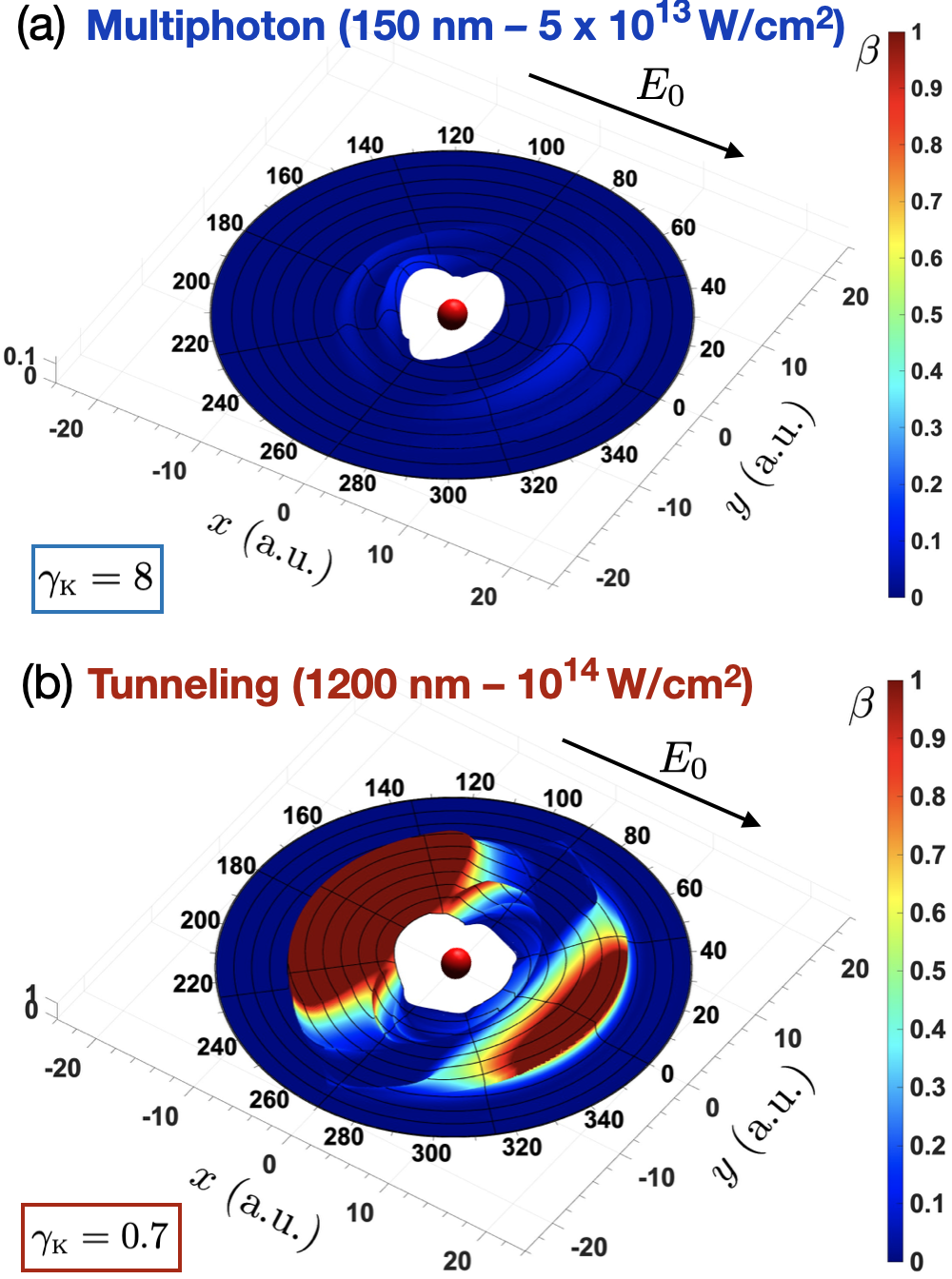
Figure 2: Tunneling parameter $\beta$ from the hydrogen ground state depending on the initial position of the trajectories in a plane containing the field. The nucleus is schematically represented by the red sphere at the origin. (a) Multiphoton case (2-cycle, 150 nm, 5$\times$10${}^{13}\,$W/cm² pulse); (b) tunneling case (1-cycle, 1200 nm, 1$\times$10${}^{14}\,$W/cm² pulse). The arrows indicate the direction of maximum electric field. The white area corresponds to the nonionizing region. See text for details.

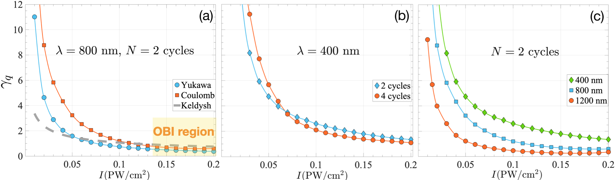
Figure 3: Value of the quantum-trajectory adiabatic parameter $\gamma_{q}$ as a function of the peak intensity in various situations. The pulse characteristics are indicated in the panels. Comparison (a) for two different potentials (Coulomb and Yukawa) and the standard Keldysh parameter ($I_{p}=0.5$ a.u.), (b) for different pulse lengths in H($1s$), and (c) for various wavelengths in H($1s$).

In the Bohmian formalism Dürr and Teufel (2009), the velocity field at a position $\bm{r}$ and time $t$ is given by $\bm{v}(\bm{r},t)=\bm{j}(\bm{r},t)/\rho(\bm{r},t)$, where $\bm{j}(\bm{r},t)={\rm\Re}\left[\Psi^{*}(\bm{r},t)\left(-i{\hbar}\nabla+{\bm{A}}(t)\right)\Psi(\bm{r},t)\right]$ is the probability flux density, ${\rm\Re}[z]$ denotes the real part of $z$, and $\rho(\bm{r},t)=|\Psi(\bm{r},t)|^{2}$ is the probability density. The velocity field is used to propagate the trajectories starting from different initial positions $\bm{r}_{0}$ in the initial state. These trajectories describe the flow of the probability density, and they enable the reconstruction of the wave function and an estimation of the energy of the system at any given time Song et al. (2017). Furthermore, they allow us to retrieve any quantum observables with high accuracy Xie et al. (2022), e.g., the ionization spectrum, the asymptotic momentum distribution, or the harmonic emission spectrum.

Using the intrinsic properties of these trajectories, one can devise complementary quantities to investigate strong-field phenomena. Specifically, we focus on the efficiency of the horizontal and vertical ionization channels (see Fig. 1) by computing the exit radius $r_{\rm ex}$ and exit time $t_{\rm ex}$ from the potential barrier for trajectories starting at different initial radii $\bm{r}_{0}$. These exit quantities are found from the condition $\Delta\mathcal{E}(t_{\rm ex})=0$, where $\Delta\mathcal{E}(t)=mv^{2}(t)/2+Q(t)$ is the gauge-independent energy difference between the energy $\mathcal{E}(t)$ of the trajectory and the barrier energy Kobe and Yang (1987). The quantum potential $Q=-\hbar^{2}/2m\{\rho^{-1/2}\nabla^{2}\rho^{1/2}\}$ is responsible for all quantum effects. In the classical limit ($Q=0$), the equations of motion reduce to the classical Hamilton-Jacobi equations, and we recover the well-known exit speed ($v=0$) Ivanov et al. (2005). The adiabatic radius, $r_{\rm ad}$, corresponds to the radius associated with perfect horizontal tunneling ionization, i.e., for a trajectory maintaining a constant energy $\mathcal{E}=-I_{p}$ and exiting the barrier at the same time $t_{\rm ex}$ and in the same direction as the trajectory under consideration. Thus, in contrast to standard approaches that define adiabatic tunneling at the maximum field strength, $r_{\rm ad}$ is a dynamical quantity that takes into account the shape of the barrier at the exit time. Finally, in the subsequent discussion, we exclusively focus on ionizing trajectories, which exhibit asymptotic freedom, i.e., $\mathcal{E}(t)\geq 0$ as $t\to\infty$.

We now define a tunneling parameter as,

$$\beta(\bm{r}_{0})\equiv\frac{r_{\rm ex}(\bm{r}_{0})-r_{0}}{r_{\rm ad}(\bm{r}_{0})-r_{0}},$$ (1)

with $0\leq\beta\leq 1$, to quantify the degree of tunneling in a trajectory starting at $\bm{r}_{0}$. For vertical ionization, $r_{\rm ex}=r_{0}$ and $\beta=0$, whereas for perfect horizontal ionization, $r_{\rm ex}=r_{\rm ad}$ and $\beta=1$. Perfect tunneling, $\beta=1$, is also assigned in the event that $r_{\rm ex}\geq r_{\rm ad}$ and for OBI, as detailed below. If a multiphoton trajectory exits the potential barrier more than once, $r_{\rm ex}$ is taken at the first exit time. As for the Keldysh parameter, this definition considers the length-gauge picture for tunneling. However, the definition of $\beta$ is not unique and could be refined further or tailored for the study of specific phenomena.

In Fig. 2, we present two-dimensional plots of $\beta(\bm{r}_{0})$ for photoionization of hydrogen as a function of the initial positions ($r_{0}<20$ a.u.) of the trajectories in the $xy$ plane. We employ two radically different pulses, describing a multiphoton case ($\gamma_{\rm\footnotesize\textsc{k}}=8$), and a tunneling situation ($\gamma_{\rm\footnotesize\textsc{k}}=0.7$) dominated by a single ionization event. The observed values of $\beta$ closely align with our expectations, exhibiting small values throughout ($0\leq\beta\leq 0.1$) for the vertical ionization case and a large region indicating tunneling for the long-wavelength scenario.

Remarkably, $\beta$ not only confirms these expectations but also provides insightful and detailed information regarding the ionization mechanism. In Fig. 2(b), it is evident that the ionization process strongly involves tunneling along the field, with larger ionization occurring from the region opposite to the direction of maximum field strength, aligning with theoretical predictions. Conversely, the multiphoton mechanism occurs orthogonal to the field, where the potential barrier is weak or nonexistent. Therefore, this mapping provides opportunities to study the angular-resolved tunneling dynamics. At large distances, the mechanism is naturally multiphoton since the trajectories exit at the early stage of the pulse, encountering an extremely broad barrier to cross, and having no time to respond to the changes in the field. Monitoring the time-dependent energy of these trajectories reveals chaotic behavior for multiphoton trajectories, while tunneling trajectories exhibit a smooth and traceable energy variation, rapidly converging to that of a classical particle ($Q\to 0$) after exiting the barrier.

The statistically averaged tunneling level of the ionization process, $\bar{\beta}={W_{0}}^{-1}\int_{\mathcal{D}}\beta(\bm{r}_{0})\rho(\bm{r}_{0},0)d^{3}\bm{r}_{0}$, is obtained by weighting $\beta(\bm{r}_{0})$ over the initial probability density carried by each ionizing trajectory Garashchuk and Rassolov (2003). Here, $\mathcal{D}$ denotes the set of ionizing trajectories and $W_{0}=\int_{\mathcal{D}}\rho(\bm{r}_{0},0)d^{3}\bm{r}_{0}$ is the total ionization probability. To design a quantity directly comparable with the Keldysh parameter, we define the quantum adiabatic parameter, $\gamma_{q}\equiv(1-\bar{\beta})/\bar{\beta}$, as the ratio between the degrees of multiphoton and tunneling ionization. This quantity has the same limits as $\gamma_{\rm\footnotesize\textsc{k}}$, i.e., $\gamma_{q}=0$ for perfect tunneling, $\gamma_{q}\to\infty$ as the ionization regime tends to multiphoton, and $\gamma_{q}=1$ for equal tunneling and multiphoton ionization ($\bar{\beta}=1/2$).

Figure 3(a) presents a comparison between $\gamma_{q}$ from H($1s$) and the Keldysh parameter for varying intensities of a 800-nm pulse. Although both parameters become unity at similar intensity levels, $\gamma_{q}$ exhibits a sharper transition between the ionization regimes, deviating from the standard $I^{-1/2}$ law. In particular, the onset of the multiphoton ionization regime is more pronounced than predicted by the Keldysh model, which is known to be inadequate in this regime Trombetta et al. (1989). To explore the sensitivity of $\gamma_{q}$ on the potential shape, we also considered the short-range Yukawa potential, $V(r)=-Z_{0}e^{-r}/r$, commonly employed to highlight tunneling effects Torlina et al. (2015). With $Z_{0}=1.94$ set to reproduce hydrogen ground-state energy ($I_{p}=0.5$ a.u.), the Keldysh parameter remains unchanged. However, $\gamma_{q}$ displays significantly more tunneling ionization for the Yukawa compared to the Coulomb potential. While this observation follows our expectations, its interpretation is not straightforward, since the tunneling barrier is, in fact, larger for the Yukawa case. This aspect, however, is counterbalanced by two factors: (i) the shorter response time of the system due to the absence of excited states, and (ii) the larger imaginary speed due to the greater height of the barrier.

In Fig. 3(b), we analyze the changes of $\gamma_{q}$ with the pulse duration, considering a 400-nm pulse with either $N=2$ or 4 cycles. A subtle difference is evident between the two pulses: $\gamma_{q}$ for the 4-cycle pulse exhibits increased multiphoton ionization at low intensity and more prominent tunneling at high intensity compared to the 2-cycle pulse. This difference is explained as follows: while both pulses reach the same field maximum at $t=0$, their satellite peaks, at $t=\pm T/2$, differ due to the different pulse envelopes. Consequently, within the multiphoton regime, vertical excitation is more prominent for the 4-cycle pulse due to the higher and additional satellite peaks. With rising intensity, the efficiency of tunneling ionization, which follows an exponential law with the field strength Ammosov et al. (1986), increases more rapidly at the satellite peaks of the 4-cycle pulse. Therefore, the difference in $\gamma_{q}$ arises mainly from the contrasting tunneling efficiency between the primary and the side peaks for each pulse. As tunneling at the primary peak becomes increasingly dominant with rising field strength, the two curves tend to converge at high intensity levels, as seen in Fig. 3(b).

Next, we computed $\gamma_{q}$ for a 2-cycle pulse at three different wavelengths: $400,~{}800$, and $1200$ nm. While the results shown in Fig. 3(c) follow the general predictions, the curves at different wavelengths are not obtained by simple rescaling, and their intensity dependence is more complex than predicted by the Keldysh model. A very interesting effect is observed for the long-wavelength pulses: $\gamma_{q}$ stops decreasing at sufficiently high intensity. This complex phenomenon might be attributed to the rising rate of change of the potential barrier with increasing intensity at a fixed wavelength near the onset of ionizing trajectories starting from the classically allowed region. This dynamical effect competes with the decrease of the tunneling time of the system. A detailed analysis of this phenomenon will be presented in a future study.

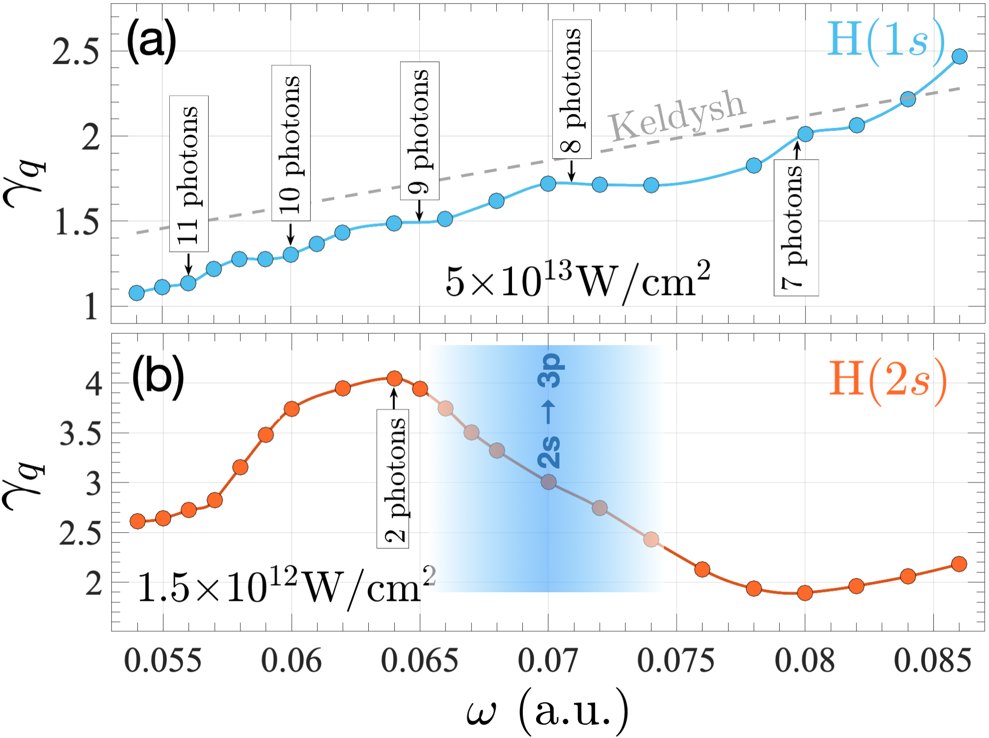
Figure 4: $\gamma_{q}$ for a $2$-cycle pulse as a function of $\omega$ starting (a) from the H($1s$) ground state compared with $\gamma_{\rm\footnotesize\textsc{k}}$, and (b) from the H($2s$) state near the $2s\to 3p$ transition energy. The frequencies for $m$-photon channel closing are indicated by arrows with the minimum number of photons to ionize also indicated. See text for details.

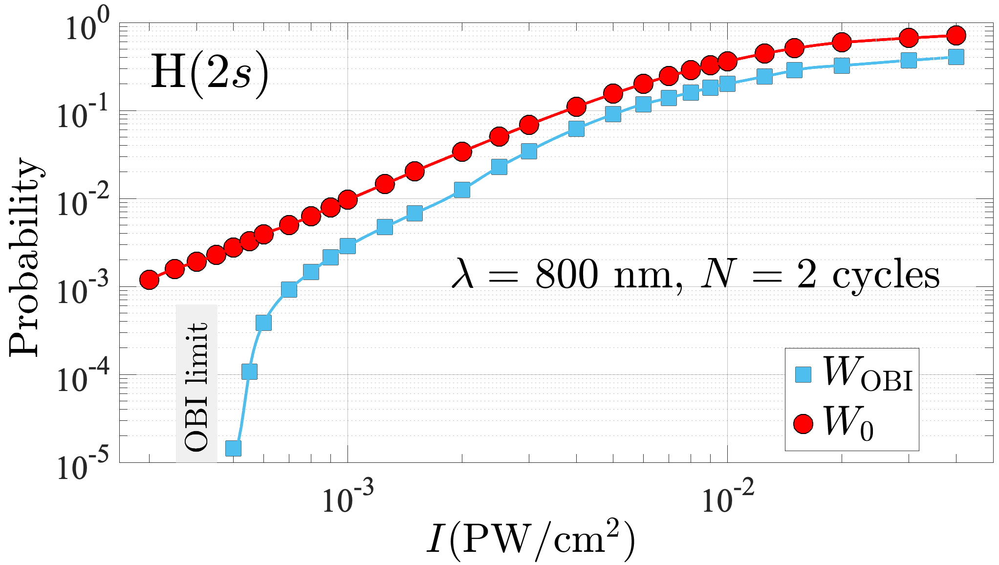
Figure 5: Total ionization probability and OBI probability starting from the H($2s$) state. The standard OBI limit is indicated on the horizontal axis.

Returning to the analysis of the frequency-dependent sensitivity of $\gamma_{q}$, Fig. 4(a) presents its variation as a function of $\omega$ for a 2-cycle pulse with $I=5\times 10^{13}\,$W/cm². While $\gamma_{q}$ exhibits an overall linear increase with $\omega$, akin to the Keldysh parameter, we observe intermittent steps during which vertical ionization ceases to progress uniformly. These distinctive steps are seen to correlate with channel-closing events Zimmermann et al. (2017), i.e., a change in the minimum number $m$ of photons needed to ionize the system. An $m$-photon channel is closed when $m\omega\leq I_{p}+U_{p}$, where $U_{p}=E_{0}^{2}/4\omega^{2}$ is the ponderomotive energy, which effectively shifts the ionization threshold upward. At channel closing, the excitation of the quasi-continuum of Rydberg states is known to suppress ionization because the characteristic time of the electron’s orbital motion is much longer than the optical cycle Topcu and Robicheaux (2012). As a result, $\gamma_{q}$ varies negligibly near channel closing. The broadening of the plateaus with increasing frequency stems from the pulse’s shortened duration, since the number $N$ of cycles is fixed.

In order to highlight the potential impact of excited states on the ionization process, we present in Fig. 4(b) results for two-photon ionization of hydrogen in the $2s$ state with varying frequencies around the $2s\to 3p$ transition. Rather than showing a steady increase, a sharp drop in $\gamma_{q}$ occurs near resonance, indicating a preference for tunneling ionization in this frequency region. This phenomenon is due to the population transfer to the $3p$ state, which temporally stabilizes the wave-packet energy and thus favors an indirect tunnel ionization, confirming findings reported in Mishima et al. (2002). As opposed to excited Rydberg states, the electron in the $3p$ orbital remains close to the nucleus, and the width of the barrier in this energy range is sufficiently large for efficient horizontal ionization to occur. With increasing intensity, the effect of resonant excitation on $\gamma_{q}$ should be less pronounced.

As a final application, we explore OBI via quantum trajectories, ionizing the H($2s$) state with a 800-nm pulse. An ionizing trajectory is classified as exhibiting OBI characteristics if either its energy $\mathcal{E}(t)$ consistently remains above the barrier, or if it exits the barrier with $\mathcal{E}(t_{\rm ex})\leq I_{p}$. This definition makes it possible to compute an OBI ionization probability, denoted as $W_{\rm OBI}$, which is compared to $W_{0}$ in Fig. 5. $W_{\rm OBI}$ experiences a sharp increase above the OBI limit corresponding to the intensity where the top of the potential barrier becomes lower than $I_{p}$. With increasing intensity, $W_{\rm OBI}$ starts to rise at a similar rate as $W_{0}$, passing through a transition phase where all trajectories starting from the classically allowed region go over the barrier. Only at an intensity about ten times larger than the OBI limit, OBI reaches a steady regime where the ratio $W_{\rm OBI}/W_{0}\approx 0.6$ remains nearly constant. We have verified that the trajectories that do not exhibit OBI characteristics correlate with ionization away from the field polarization.

In conclusion, we showed that quantum trajectories can be used as a powerful tool to investigate strong-field phenomena and explore the electron dynamics beneath a potential barrier in the strong-field ionization of atoms. As a result, we obtain a comprehensive and consistent framework to analyze the mechanisms of multiphoton and tunneling ionization in atoms. This methodology could open the way to explore novel dynamical effects and advance theoretical models. Such an approach could also be applied to study, e.g., the dynamics of recombining trajectories in high-harmonic generation (HHG) Ishii et al. (2008); Dong et al. (2020); Petrakis et al. (2021); Piper (2022), the process of frustrated tunneling ionization Nubbemeyer et al. (2008), or the influence of chirality on the tunnel-ionization dynamics Bloch et al. (2021).

This work was supported by the NSF under grants No. PHY-2012078 (N.D.) and No. PHY-2110023 (K.B.).

References

- Paul et al. (2001) P. M. Paul, E. S. Toma, P. Breger, G. Mullot, F. Augé, P. Balcou, H. G. Muller, and P. Agostini, Science 292, 1689 (2001).
- Li et al. (2020) J. Li, J. Lu, S. Han, J. Li, Y. Wu, H. Wang, S. Ghimire, and Z. Chang, Nat. Commun. 11, 2748 (2020).
- Maroju et al. (2020) P. K. Maroju, C. Grazioli, M. Di Fraia, M. Moioli, D. Ertel, H. Ahmadi, O. Plekan, P. Finetti, E. Allaria, L. Giannessi, et al., Nature 578, 386 (2020).
- Zhang et al. (2017) C. Zhang, V. Bucklew, P. Edwards, C. Janisch, and Z. Liu, Opt. Lett. 42, 502 (2017).
- Stewart et al. (2023) G. A. Stewart, P. Hoerner, D. A. Debrah, S. K. Lee, H. B. Schlegel, and W. Li, Phys. Rev. Lett. 130, 083202 (2023).
- Isinger et al. (2017) M. Isinger, R. J. Squibb, D. Busto, S. Zhong, A. Harth, D. Kroon, S. Nandi, C. L. Arnold, M. Miranda, J. M. Dahlström, et al., Science 358, 893 (2017).
- Sainadh et al. (2019) U. S. Sainadh, H. Xu, X. Wang, A. Atia-Tul-Noor, W. C. Wallace, N. Douguet, A. Bray, I. Ivanov, K. Bartschat, A. Kheifets, et al., Nature 568, 75 (2019).
- Popruzhenko (2014) S. V. Popruzhenko, J. Phys. B: At. Mol. Opt. Phys. 47, 204001 (2014).
- Faisal (1973) F. H. M. Faisal, J. Phys. B: At. Mol. Opt. Phys. 6, L89 (1973).
- Reiss (1980) H. R. Reiss, Phys. Rev. A 22, 770 (1980).
- Agostini and DiMauro (2012) P. Agostini and L. F. DiMauro, in Adv. At. Mol. Opt. Phys., edited by P. Berman, E. Arimondo, and C. Lin (Academic Press, 2012), vol. 61, pp. 117–158.
- Smirnova et al. (2008) O. Smirnova, M. Spanner, and M. Ivanov, Phys. Rev. A 77, 033407 (2008).
- Torlina and Smirnova (2012) L. Torlina and O. Smirnova, Phys. Rev. A 86, 043408 (2012).
- Delone and Krainov (2000) N. B. Delone and V. P. Krainov, Above-Threshold Ionization of Atoms (Springer Berlin Heidelberg, Berlin, Heidelberg, 2000), pp. 151–187.
- Ivanov et al. (2005) M. Y. Ivanov, M. Spanner, and O. Smirnova, J. Mod. Opt. 52, 165 (2005).
- Keldysh (1965) L. Keldysh, JETP 20, 1307 (1965).
- Topcu and Robicheaux (2012) T. Topcu and F. Robicheaux, Phys. Rev. A 86, 053407 (2012).
- Delone and Krainov (1998) N. B. Delone and V. P. Krainov, Phys. Usp. 41, 469 (1998).
- Reiss (2010) H. R. Reiss, Phys. Rev. A 82, 023418 (2010).
- Trombetta et al. (1989) F. Trombetta, S. Basile, and G. Ferrante, Phys. Rev. A 40, 2774 (1989).
- Mishima et al. (2002) K. Mishima, M. Hayashi, J. Yi, S. H. Lin, H. L. Selzle, and E. W. Schlag, Phys. Rev. A 66, 033401 (2002).
- Chetty et al. (2022) D. Chetty, R. D. Glover, X. M. Tong, B. A. deHarak, H. Xu, N. Haram, K. Bartschat, A. J. Palmer, A. N. Luiten, P. S. Light, et al., Phys. Rev. Lett. 128, 173201 (2022).
- Karamatskou et al. (2013) A. Karamatskou, S. Pabst, and R. Santra, Phys. Rev. A 87, 043422 (2013).
- Douguet and Bartschat (2018) N. Douguet and K. Bartschat, Phys. Rev. A 97, 013402 (2018).
- Krainov (1995) V. P. Krainov, J. Nonlin. Opt. Phys. & Mat. 04, 775 (1995).
- Schuricke et al. (2011) M. Schuricke, G. Zhu, J. Steinmann, K. Simeonidis, I. Ivanov, A. Kheifets, A. N. Grum-Grzhimailo, K. Bartschat, A. Dorn, and J. Ullrich, Phys. Rev. A 83, 023413 (2011).
- Arbó et al. (2008) D. G. Arbó, J. E. Miraglia, M. S. Gravielle, K. Schiessl, E. Persson, and J. Burgdörfer, Phys. Rev. A 77, 013401 (2008).
- Popruzhenko et al. (2008) S. V. Popruzhenko, V. D. Mur, V. S. Popov, and D. Bauer, Phys. Rev. Lett. 101, 193003 (2008).
- Wang et al. (2019) R. Wang, Q. Zhang, D. Li, S. Xu, P. Cao, Y. Zhou, W. Cao, and P. Lu, Opt. Express 27, 6471 (2019).
- Zheltikov (2016) A. M. Zheltikov, Phys. Rev. A 94, 043412 (2016).
- Heldt et al. (2023) T. Heldt, J. Dubois, P. Birk, G. D. Borisova, G. M. Lando, C. Ott, and T. Pfeifer, Phys. Rev. Lett. 130, 183201 (2023).
- Xie et al. (2022) W. Xie, M. Li, Y. Zhou, and P. Lu, Phys. Rev. A 105, 013119 (2022).
- Ni et al. (2016) H. Ni, U. Saalmann, and J.-M. Rost, Phys. Rev. Lett. 117, 023002 (2016).
- Camus et al. (2017) N. Camus, E. Yakaboylu, L. Fechner, M. Klaiber, M. Laux, Y. Mi, K. Z. Hatsagortsyan, T. Pfeifer, C. H. Keitel, and R. Moshammer, Phys. Rev. Lett. 119, 023201 (2017).
- Salières et al. (2001) P. Salières, B. Carré, L. L. Déroff, F. Grasbon, G. G. Paulus, H. Walther, R. Kopold, W. Becker, D. B. Milošević, A. Sanpera, et al., Science 292, 902 (2001).
- Yang and Robicheaux (2016) B. C. Yang and F. Robicheaux, Phys. Rev. A 93, 053413 (2016).
- Tan et al. (2021) J. Tan, Y. Zhou, S. Xu, Q. Ke, J. Liang, X. Ma, W. Cao, M. Li, Q. Zhang, and P. Lu, Opt. Expr. 29, 37927 (2021).
- Krause et al. (1992) J. L. Krause, K. J. Schafer, and K. C. Kulander, Phys. Rev. Lett. 68, 3535 (1992).
- Corkum (1993) P. B. Corkum, Phys. Rev. Lett. 71, 1994 (1993).
- Corkum and Krausz (2007) P. B. Corkum and F. Krausz, Nat. Phys. 3, 381 (2007).
- Perelomov et al. (1966) A. M. Perelomov, V. S. Popov, and M. V. Terent’ev, Sov. J. Expt. Theor. Phy. (JETP) 23, 924 (1966).
- Hack et al. (2021) S. Hack, S. Majorosi, M. G. Benedict, S. Varró, and A. Czirják, Phys. Rev. A 104, L031102 (2021).
- Dürr and Teufel (2009) D. Dürr and S. Teufel, Bohmian Mechanics (Springer Berlin Heidelberg, 2009).
- Botheron and Pons (2010) P. Botheron and B. Pons, Phys. Rev. A 82, 021404 (2010).
- Benseny et al. (2014) A. Benseny, G. Albareda, A. S. Sanz, J. Mompart, and X. Oriols, Eur. J. Phys. D 68, 286 (2014).
- Jooya et al. (2015) H. Z. Jooya, D. A. Telnov, P.-C. Li, and S.-I. Chu, Phys. Rev. A 91, 063412 (2015).
- Zimmermann et al. (2016) T. Zimmermann, S. Mishra, B. R. Doran, D. F. Gordon, and A. S. Landsman, Phys. Rev. Lett. 116, 233603 (2016).
- Douguet et al. (2016) N. Douguet, A. N. Grum-Grzhimailo, E. V. Gryzlova, E. I. Staroselskaya, J. Venzke, and K. Bartschat, Phys. Rev. A 93, 033402 (2016).
- Song et al. (2017) Y. Song, Y. Yang, F. Guo, and S. Li, J. Phys. B: At. Mol. Opt. Phys. 50, 095003 (2017).
- Kobe and Yang (1987) D. H. Kobe and K.-H. Yang, Eur. J. Phys. 8, 236 (1987).
- Garashchuk and Rassolov (2003) S. Garashchuk and V. A. Rassolov, J. Chem. Phys. 118, 2482 (2003).
- Torlina et al. (2015) L. Torlina, F. Morales, J. Kaushal, I. Ivanov, A. Kheifets, A. Zielinski, A. Scrinzi, H. G. Muller, S. Sukiasyan, M. Ivanov, et al., Nat. Phys. 11, 503 (2015).
- Ammosov et al. (1986) M. V. Ammosov, N. B. Delone, and V. P. Krainov, in High Intensity Laser Processes, edited by J. A. Alcock, International Society for Optics and Photonics (SPIE, 1986), vol. 0664, pp. 138 – 141.
- Zimmermann et al. (2017) H. Zimmermann, S. Patchkovskii, M. Ivanov, and U. Eichmann, Phys. Rev. Lett. 118, 013003 (2017).
- Ishii et al. (2008) N. Ishii, A. Kosuge, T. Hayashi, T. Kanai, J. Itatani, S. Adachi, and S. Watanabe, Opt. Express 16, 20876 (2008).
- Dong et al. (2020) W. Dong, H. Hu, and Z. Zhao, Opt. Express 28, 22490 (2020).
- Petrakis et al. (2021) S. Petrakis, M. Bakarezos, M. Tatarakis, E. P. Benis, and M. A. Papadogiannis, Sci. Rep. 11, 23882 (2021).
- Piper (2022) A. Piper, The Strong Field Simulator: Studying Quantum Trajectories in Classical Fields (ProQuest Dissertations & Theses Global, 2022).
- Nubbemeyer et al. (2008) T. Nubbemeyer, K. Gorling, A. Saenz, U. Eichmann, and W. Sandner, Phys. Rev. Lett. 101, 233001 (2008).
- Bloch et al. (2021) E. Bloch, S. Larroque, S. Rozen, S. Beaulieu, A. Comby, S. Beauvarlet, D. Descamps, B. Fabre, S. Petit, R. Taïeb, et al., Phys. Rev. X 11, 041056 (2021).