Merger-driven multi-scale ICM density perturbations: testing cosmological simulations and constraining plasma physics

Abstract

The hot intracluster medium (ICM) provides a unique laboratory to test multi-scale physics in numerical simulations and probe plasma physics. Utilizing archival Chandra observations, we measure density fluctuations in the ICM in a sample of 80 nearby ($z\lesssim 1$) galaxy clusters and infer scale-dependent velocities within regions affected by mergers ($r<$ $R_{\rm 2500c}$), excluding cool-cores. Systematic uncertainties (e.g., substructures, cluster asymmetries) are carefully explored to ensure robust measurements within the bulk ICM. We find typical velocities $\sim 220$ ($300$) km s^-1 in relaxed (unrelaxed) clusters, which translate to non-thermal pressure fractions $\sim 4$ ($8$) per cent, and clumping factors $\sim 1.03$ ($1.06$). We show that density fluctuation amplitudes could distinguish relaxed from unrelaxed clusters in these regions. Comparison with density fluctuations in cosmological simulations shows good agreement in merging clusters. Simulations underpredict the amplitude of fluctuations in relaxed clusters on length scales $<0.75$ $R_{\rm 2500c}$, suggesting these systems are most sensitive to “missing” physics in the simulations. In clusters hosting radio halos, we examine correlations between gas velocities, turbulent dissipation rate, and radio emission strength/efficiency to test turbulent re-acceleration of cosmic ray electrons. We measure a weak correlation, driven by a few outlier clusters, in contrast to some previous studies. Finally, we present upper limits on effective viscosity in the bulk ICM of 16 clusters, showing it is systematically suppressed by at least a factor of 8, and the suppression is a general property of the ICM. Confirmation of our results with direct velocity measurements will be possible soon with XRISM.

1 Introduction

Galaxy clusters are the most massive gravitationally-bound systems in the universe and continue to grow via hierarchical mergers and continuous accretion of matter from the intergalactic medium. These accretion processes are the dominant drivers of gas dynamics within the hot ($T\sim 10^{7.5}$ K) intracluster medium (ICM) outside the innermost regions (e.g., Walker et al., 2019; Heinrich et al., 2021; ZuHone & Su, 2022) that are often affected by feedback from central supermassive black holes (see, e.g., Hlavacek-Larrondo et al., 2022, for a recent review). Probing turbulent and bulk motions within the ICM is crucial for understanding energy partition during large-scale structure evolution, astrophysical processes that drive the evolution of galaxies within the ICM, and plasma physics, yet direct measurements of these motions remain challenging (for exceptions, see, e.g., Gatuzz et al., 2023; Sanders et al., 2020; Hitomi Collaboration et al., 2018; Sanders & Fabian, 2013). Directly resolving bulk and turbulent velocities of the hot gas in galaxy clusters, groups, and massive galaxies will soon be possible with the recently-launched XRISM satellite (XRISM Science Team, 2020).

While waiting for data from X-ray microcalorimeters, such as XRISM, NewAthena (Barret et al., 2020) and LEM (Kraft et al., 2022), to become available, indirect techniques have been used to constrain ICM velocities, including resonant scattering (e.g., Hitomi Collaboration et al., 2017; Ogorzalek et al., 2017), inference from metal abundance distributions (Rebusco et al., 2005), shock widths (Nulsen et al., 2013), and X-ray surface brightness or Sunyaev-Zel’dovich fluctuations (e.g., Schuecker et al., 2004; Churazov et al., 2012; Zhuravleva et al., 2015; Walker et al., 2015; Romero et al., 2023). This last method is particularly attractive as it provides characteristic velocity amplitudes as a function of spatial scale (or wavenumber) — information that is difficult to extract, even from direct velocity measurements through Doppler shifts.

The X-ray surface brightness method utilizes a relation between the scale-dependent amplitude (related to a power spectrum) of gas density fluctuations, $\left(\delta\rho/\rho\right)_{k}$, and the one-dimensional characteristic velocity, $V_{\text{1D,k}}$. This method has previously been calibrated using relaxed clusters from non-radiative cosmological simulations (Zhuravleva et al., 2014b) and idealized Coma-like cluster simulations (Gaspari et al., 2014). It was first applied to a sample of the brightest cores of relaxed clusters to measure velocity power spectra (e.g., Zhuravleva et al., 2014a; Zhuravleva et al., 2018). Recently, this relationship was verified for unrelaxed objects in cosmological simulations (Simonte et al., 2022; Zhuravleva et al., 2023), showing that the correlation is still valid, though the scatter is larger by a factor of $\sim 2$ compared to relaxed systems (Zhuravleva et al., 2023). High-resolution idealized simulations of stratified turbulence (Mohapatra et al., 2020, 2021) showed that the relationship is more complicated and depends on the level of stratification, turbulence driving, and pressure/entropy scale height of the system, which could explain the scatter in the simplified relation.

Using mostly imaging data from XMM-Newton, the technique has been applied to unrelaxed objects and regions outside of cool-cores (Eckert et al., 2017; Zhang et al., 2022), where gas dynamics are driven mainly by cluster mergers. The relatively large PSF of that telescope, however, limits measurements to rather large scales. Given high-resolution images of galaxy clusters obtained with Chandra, this method can provide velocity measurements on scales small enough to test plasma effects and small-scale physics in simulations. Luckily, after nearly 25 years of operations, the Chandra archive contains enough data to measure these velocities in a large sample of clusters.

Velocity measurements outside of cool-cores open up a variety of phenomena that can be studied. For example, turbulence in the ICM is theorized to be linked to diffuse synchrotron emission from giant radio halos, mostly found in dynamically disturbed clusters (e.g., Cassano et al., 2010). The GeV cosmic-ray electrons (CRe) powering the radio emission in halos are likely associated with 2nd-order Fermi acceleration (e.g., Brunetti & Lazarian, 2007; Petrosian & Bykov, 2008; van Weeren et al., 2019) of a seed CRe population. Measurements of turbulent velocities and their correlation with the radio emission strength could, therefore, provide valuable insights into the CRe acceleration mechanisms.

Additionally, the ICM is threaded by a (likely) tangled magnetic field with $B\sim$ a few $\mu G$. Although the magnetic pressure is small compared to the thermal pressure, the field can significantly alter the ICM microphysics, including the ICM’s transport properties (e.g., Schekochihin & Cowley, 2006; Kunz et al., 2022; Arzamasskiy et al., 2023). Multi-scale velocity measurements to scales close to the Coulomb mean-free-path of particle interactions ($\lambda_{\text{mfp}}$) are crucial for understanding the ICM as a weakly-collisional high-$\beta$ plasma. Since $\lambda_{\text{mfp}}$ typically increases with the radius in the ICM, probing microphysical scales with observations is most promising in regions outside dense cluster cores.

Finally, the partition of energy during matter accretion onto virialized halos and cluster mergers also depends on the poorly known microphysics of the hot plasma in the ICM. Measuring gas motions outside cluster cores, one can directly probe what fraction of gravitational energy converts into thermal and kinetic energies. The latter contribution also biases cluster mass measurements based on the assumption of hydrostatic equilibrium (e.g., Lau et al., 2009; Nelson et al., 2014a; Vazza et al., 2018). Measuring the non-thermal pressure and demonstrating that it is responsible for the mass bias are important for a few percent-level precision cluster cosmology with X-ray and SZ techniques.

In this work, we will, for the first time, measure ICM gas velocities across a range of scales using the density fluctuations technique in a large sample of galaxy clusters within a cosmologically-interesting region of radius of $R_{\rm 2500c}$ using archival Chandra data. The high spatial resolution of Chandra allows us to measure velocities on smaller scales (and a broader range of scales) than studied previously. We will probe gas dynamics driven by mergers and large-scale structure evolution, minimizing the effects of AGN feedback and gas cooling. We assume a flat $\Lambda$CDM cosmology with $h=0.7$ and $\Omega_{\rm m}=0.3$. $R_{n\text{c}}$ is defined as the cluster-centric radius within which the average density is $n$ times the critical density of the universe at the cluster’s redshift.

In Section 2, we describe our sample of clusters, image processing techniques, and power spectral analysis methods. In Section 3, we present individual and averaged measurements of $\left(\delta\rho/\rho\right)_{k}$, the characteristic ICM gas velocity $V_{\text{1D,k}}$, and place limits on the ICM clumping factor and scale-independent characteristic velocity. Section 4.1.1 discusses these constraints in relation to cosmological simulations. Finally, Section 4.2 focuses on relevant plasma physics, namely, testing the turbulent re-acceleration mechanism of CRe and constraining transport properties in the bulk ICM.

2 Sample selection and data analysis

We aim to measure the power spectra of hot gas density fluctuations down to the smallest possible scales in a large sample of galaxy clusters. The Chandra X-ray Observatory is best-suited for our goal as it offers the highest angular resolution. We select systems where archival Chandra observations cover (nearly) the entirety of the cluster within a projected radius of $R_{\rm 2500c}$ from the cluster center, as determined from X-ray surface brightness contours at the same radius. The clusters are also brighter than the background level by at least a factor of two in this region. To have a sufficient number of photons in the X-ray images, we further require the total exposure time of each cluster to be greater than 100 ks. However, we also examine a few bright clusters below this threshold. Our final sample totals 80 clusters, with Chandra ObsIDs and cleaned exposure times presented in Table LABEL:tab:observations. We collected measured total masses ($M_{\rm 2500c}$) and characteristic radii ($R_{\rm 2500c}$) from the literature, summarizing their values and corresponding references in Table LABEL:tab:parameters. Figure 1 summarizes our sample. Most clusters in our sample have masses ($M_{\rm 2500c}$) between $\sim 8\times 10^{13}$ and $\sim 10^{15}$ $M_{\odot}$, and have redshifts between $\sim 0.05$ and $\sim 0.5$.

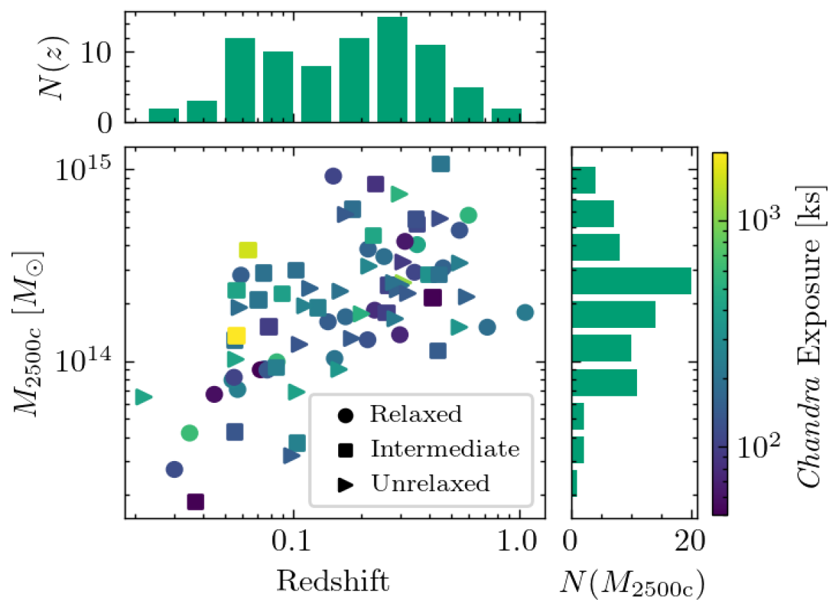
Figure 1: Our sample of 80 galaxy clusters in which we measure density fluctuation power spectra: $M_{2500c}$ vs. cluster redshift. Marker shapes indicate cluster morphology: “relaxed” (circles, cool-core systems with no signs of recent mergers), “intermediate” (squares, evidence of a minor merger), or “unrelaxed” (triangles, recent or ongoing major merger, no cool-cores), based on a literature review and visual inspection of the X-ray images, see Section 2.2 for details. Color indicates flare-removed (clean) Chandra exposure time in ks. Top: histogram of cluster redshifts. Right: histogram of cluster masses within $R_{\rm 2500c}$.

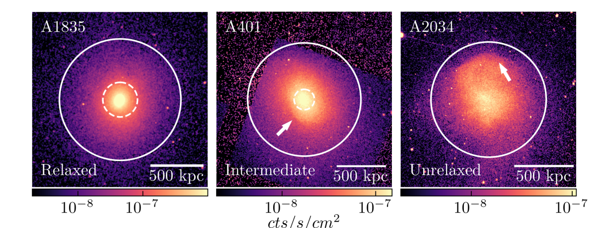
Figure 2: Representative examples of clusters from relaxed, intermediate, and unrelaxed subsamples. Exposure-corrected Chandra X-ray (0.5-3.5 keV band) images are shown, lightly smoothed with a Gaussian for display purposes. Solid white circles represent $R_{\rm 2500c}$, while dashed circles mark the cool-core radius if the cluster has one. A1835 is a relaxed, cool-core cluster that does not show any signs of mergers (Schmidt et al., 2001; Govoni et al., 2009). A401 is a cool-core cluster, however, it is undergoing a merger as evidenced by the sloshing cold front to the south (white arrow), the proximity of the cluster to A399, and the presence of a giant radio halo (Murgia et al., 2010). For these reasons, we place it in the intermediate category. A2034 is a clear example of an unrelaxed, merging cluster as it lacks a cool-core, shows irregular morphology, contains a merger shock north of the cluster center (white arrow Owers et al., 2013), and hosts a radio halo (Botteon et al., 2022).

2.1 Initial data processing

The data for each cluster are reprocessed using the standard methods described in Vikhlinin et al. (2005), implementing scripts from ciao version 4.14. Event lists are reprocessed using CalDB version 4.9.7. Background flares are removed by filtering lightcurves using the lc_sigma_clip script. Non-X-Ray background files are created using combined products of the blanksky and readout_bkg routines. Event lists are restricted to the 0.5-3.5 keV band, where X-ray emissivity is almost independent of temperature for typical temperatures of galaxy clusters (Forman et al., 2007, see their Figure 1). The resultant event lists are combined using the merge_obs script, creating mosaic images of X-ray counts, background, a weighted instrument exposure map, and an exposure-weighted point-spread-function (PSF) map. A selection of exposure-corrected images of galaxy clusters from our sample is presented in Figure 2.

2.2 Classification of galaxy clusters

Based on these X-ray images and a literature review, we classify clusters in our sample into “relaxed”, “intermediate”, and “unrelaxed” systems. Relaxed clusters have cool-cores, exhibit regular spherical or elliptical morphologies in X-rays, and show no signs of recent or ongoing mergers. Most intermediate clusters maintained their cool-cores and showed evidence of minor mergers (e.g., gas sloshing). Clusters that are undergoing a merger but show regular morphology (e.g., A1689, which has spherical X-ray morphology and a weak cool-core, but hosts a radio halo (Vacca et al., 2011) and is likely undergoing a merger along the line-of-sight based on the galaxy redshift distribution (Girardi et al., 1997)) are also included into the “intermediate” category. Unrelaxed clusters are generally non-cool-core and show clear signs of ongoing major mergers, including shock fronts and “bullet-like” morphologies. Representative examples of these three categories are shown in Figure 2. While the divisions between relaxed and intermediate clusters, and between intermediate and unrelaxed clusters, are somewhat uncertain, the relaxed and unrelaxed subsamples are likely well separated in terms of merger effects. The “relaxed”, “intermediate”, and “unrelaxed” subsamples include 24, 30, and 26 clusters, respectively.

2.3 Deprojection analysis

To obtain radial profiles of gas density, temperature, and abundance of heavy elements for a subsample of galaxy clusters discussed in Section 4.2.2, we extract projected spectra in a set of radial annuli. These spectra are deprojected using a flavor of the onion-peeling technique described by Churazov et al. (2003). The resulting deprojected spectra are fit in the broad $0.6-8$ keV band using XSPEC code (Arnaud, 1996) and APEC plasma model (Smith et al., 2001) based on AtomDB (Foster et al., 2012) version 3.0.9. The abundance of heavy elements is fixed at 0.5 relative to Solar abundances of heavy elements taken from Anders & Grevesse (1989) in the fitting. However, we verify that treating the abundance as a free parameter does not affect the measured density and temperature profiles.

2.4 Residual images

Point sources in the X-ray images are identified via the wavdetect tool (accounting for the PSF), visually confirmed, and masked. The exposure-corrected and background-subtracted image is then radially binned into logarithmically-spaced annuli to create a surface brightness profile, $S(r)$, as a function of the projected radius $r$, for each cluster. We check that X-ray emission from each cluster is observable above the background within the region of interest. We then perform a least-squares fit of this profile to a spherically symmetric double $\beta$-model:

$$S(r)=\sum_{n=1}^{2}S_{n}\left[1+\left(\frac{r}{r_{\text{c},n}}\right)^{2}\right]^{-3\beta_{n}+0.5},\\$$ (1)

where the free parameters are the surface brightness normalization $S_{n}$, core radius $r_{\text{c},n}$, and the $\beta_{n}$ parameter, and $n$ is the number of components (one or two $\beta-$models). This fitted $\beta$-model is used as the unperturbed surface brightness model for each cluster. For unrelaxed clusters that do not have the excess central emission associated with a cooling flow, the second $\beta$-model component, $S_{2}$, is fixed to zero. To obtain the images of X-ray surface brightness fluctuations (residual images), we divide the initial cluster images by their best-fitting models.

Many clusters exhibit an elliptical X-ray morphology reflecting the underlying gravitational potential of the dark matter halo (e.g., Umetsu et al., 2018; Gonzalez et al., 2021). We correct our fitted $\beta$-model to better reflect this ellipticity by performing a Levenberg-Marquardt two-dimensional fit of the exposure-corrected image to an elliptical $\beta$-model, where the projected radius $r$ in equation (1) has been replaced with the elliptical radius $r_{\text{e}}$, with additional free parameters $\epsilon$ (ellipticity) and $\theta$ (orientation). The ratio of the best-fitting elliptical and spherical models is then used to correct the spherically symmetric $\beta$-model described above.

Additionally, the gas density distribution in dynamically disturbed clusters is often asymmetric. Assuming a spherically- or even elliptically-symmetric underlying model in such systems can significantly bias the measurement of density fluctuations on large scales. To model an asymmetric cluster atmosphere, we “patch” the $\beta$-model on large spatial scales following Zhuravleva et al. (2015). For details, see Appendix A. In short, the residual image is smoothed by a Gaussian with a large width to obtain a correction for the large-scale deviations. The unperturbed model (normalized by the image mask smoothed on the same scale) is then multiplied by this correction to get a patched model. This “patched” model effectively removes the large-scale asymmetries in residual images. We caution that the choice of patching scale is non-obvious. In our work, we calculate the power spectrum assuming several patching scales to determine which scale visually removes the asymmetry from the residual image. Our analysis only includes measurements of $\left(\delta\rho/\rho\right)_{k}$ at scales that are unaffected by the choice of patching scale.

2.5 Power spectral analysis

To measure the power spectra of density fluctuations from the observed residual images, we follow the analysis steps described by Churazov et al. (2012). We employ the $\Delta$-variance method (Arevalo et al., 2012) to measure the power spectrum of surface brightness fluctuations, $P_{\text{2D}}(k)$, in the residual image. The method is tuned for the non-periodic data with gaps and is best suited for power spectra that are smooth functions. In brief, given a masked image $I$ of the background-subtracted X-ray counts and the exposure map $E$ (product of the Chandra exposure map, unperturbed density model, and mask $M$), the power spectrum ($P_{\text{2D}}(k)$) of the residual image at a wavenumber $k$ is given by

$$P_{\text{2D}}(k)=\frac{\Sigma I_{k}^{2}}{\Sigma M}\frac{1}{\epsilon^{2}\pi k^{2}},$$ (2)

where

$$I_{k}=\left(\frac{G_{k_{1}}\ast I}{G_{k_{1}}\ast E}-\frac{G_{k_{2}}\ast I}{G_{k_{2}}\ast E}\right)M$$ (3)

with Gaussian kernels $G_{k_{1}}$ and $G_{k_{2}}$ of widths $\frac{0.225}{k}\sqrt{1+\epsilon}$ and $\frac{0.225}{k\sqrt{1+\epsilon}}$, where $\epsilon\ll 1$.

We can deproject the 2D power spectrum of surface brightness fluctuations, $P_{\text{2D}}(k)$, to a 3D power spectrum of X-ray emissivity fluctuations, $P_{\text{3D}}(k)$, and obtain the amplitude of density fluctuations at each wavenumber, i.e., $\left(\delta\rho/\rho\right)_{k}=\sqrt{4\pi P_{\text{3D}}(k)k^{3}}$. Assuming that density fluctuations are a homogeneous and isotropic random field, $P_{\text{2D}}$ is related to $P_{\text{3D}}$ as

$$P_{\text{2D}}(k)\approx 4P_{\text{3D}}(k)\int|W(k_{\text{z}})|^{2}dk_{\text{z}},$$ (4)

where $W(k_{\text{z}})$ is the Fourier transform of the normalized emissivity distribution along the line of sight. The emissivity, and therefore the deprojection factor (integral in equation (4)), depends on the projected radius $r$. We calculate this deprojection factor at each line of sight and include it in the exposure map from equation (3).

We measure $\left(\delta\rho/\rho\right)_{k}$ at each wavenumber $k$ and relate it to the characteristic velocity of subsonic gas motions through the statistical relationship

$$\left(\frac{\delta\rho}{\rho}\right)_{k}=\eta\left(\frac{V_{\text{1D,k}}}{c_{\text{s}}}\right),$$ (5)

where $V_{\text{1D,k}}$ is a scale-dependent characteristic one-dimensional velocity of gas motions in the ICM, $c_{\text{s}}$ is the sound speed and $\eta$ is a proportionality coefficient. Recently updated analysis of gas fluctuations in galaxy clusters from cosmological numerical simulations (Zhuravleva et al., 2023, hereafter Z23) confirmed a strong correlation between velocities and density fluctuations, finding that $\eta$ varies slightly depending on the cluster dynamical state. Note that this result differs from the conclusions of Simonte et al. (2022), who filter the velocity field in order to separate bulk and turbulent motions. Given the difficulty in unambiguously defining the filtering scale (both in observations and simulations), we conservatively measure the whole velocity field. Following Z23, who average $\eta$ between scales of 60 to 300 kpc, our adopted values for $\eta$ are summarized in Table 1. In the near future, this relationship will be tested using direct measurements of the turbulent velocity dispersion with XRISM. The first such measurement performed by Hitomi was broadly consistent with $\eta\approx 1$ in the Perseus cluster core (Hitomi Collaboration et al., 2018).

Dynamical State	Relaxed	Intermediate	Unrelaxed
$\eta$	$0.98\pm 0.14$	$1.04\pm 0.18$	$1.16\pm 0.30$

Table 1: Adopted values for the proportionality coefficient $\eta$, from (Z23).

As our goal is to probe merger-driven gas motions and density fluctuations, we derive the density fluctuation power spectrum within a cluster-centric projected radius of $R_{\rm 2500c}$, where the effect of the non-X-ray-background is minimized. We omit (mask) cool-cores where appropriate, as these are often perturbed by AGN activity (e.g., Heinrich et al., 2021; Walker et al., 2018) and strong cooling (Fabian, 1994; Hudson et al., 2010). We define $R_{\text{cool}}$ as the radius within which the gas cooling time $t_{\text{cool}}$ is less than the age of the universe $t_{\text{age}}(z)$.

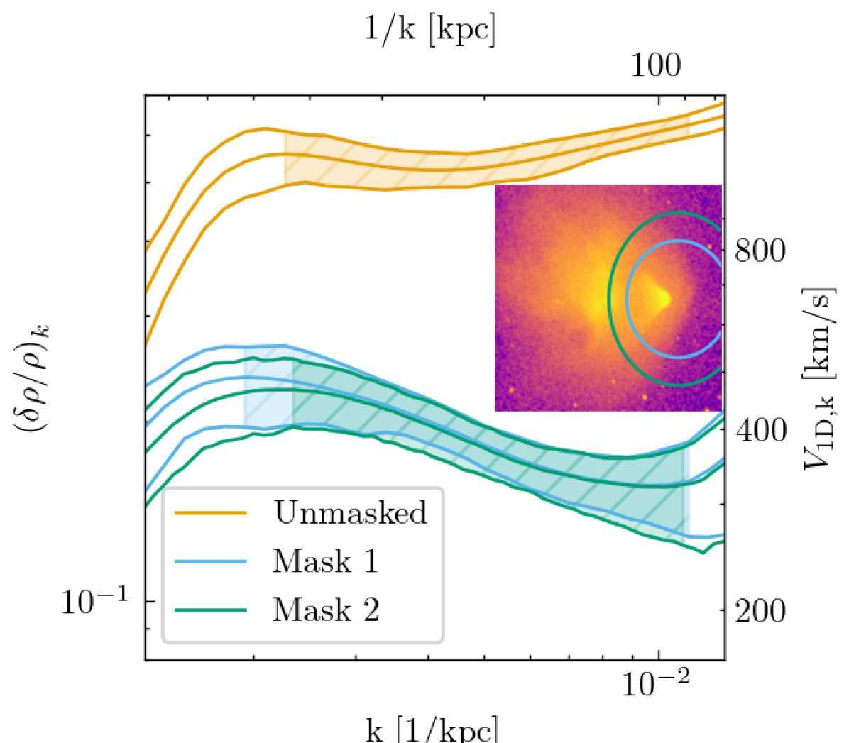
Figure 3: Effect of bright substructures on measurements of $\left(\delta\rho/\rho\right)_{k}$ in the Bullet cluster. Solid lines show the mean value of $\left(\delta\rho/\rho\right)_{k}$, corrected for Poisson noise and effects of the Chandra PSF, with $1\sigma$ uncertainties (upper and lower limits). Shaded regions show wavenumbers where the measurement is unaffected by observational effects. Inset shows the exposure-corrected image of the $R_{\rm 2500c}$ region. The orange spectrum is measured in the whole region, while blue and green spectra are measured when their respective ellipses (see inset) are excluded. The exclusion of the blue ellipse is sufficient for characterizing fluctuations in the bulk ICM.

2.6 Bright substructures

Galaxy clusters continuously grow through mergers and often exhibit bright substructures that can dominate the signal if not properly excluded. Our primary goal is to characterize volume filling (bulk) gas perturbations. As such, for each cluster with prominent substructures, we produce two power spectra: one with substructures included and one without. Each cluster with identifiable substructures is tested to determine the region size that sufficiently masks each feature. Figure 3 provides an example of this test on the Bullet cluster. This cluster is undergoing a major merger in the plane of the sky that is responsible for the bright cold front (the eponymous “bullet”), the remnant of the infalling system’s cool-core, and the sharp surface brightness discontinuity to the west of the “bullet”, a bow shock (Markevitch et al., 2002). We first calculate $\left(\delta\rho/\rho\right)_{k}$ for the entire cluster within $R_{\rm 2500c}$, shown in Figure 3 as the orange spectrum. The blue and green spectra are then calculated after masking their respective regions shown on the inset. One can see the spectrum significantly decreases when the blue region is masked, but shows little change in the case of the larger green region. Therefore, we conclude the blue region is sufficient to remove the effect of these substructures on the spectrum as a whole. The slight difference between the blue and green spectra at large spatial scales is due to the lower sampling of these scales when the region size is increased. In our final analysis, we only include scales that are largely unaffected by the choice of masked region.

2.7 Limits on observable scales

Each cluster must be carefully examined to determine which length scales are reliably probed within $R_{\rm 2500c}$, given the available data. On large scales, our measurement is limited by the region size. When $1/k$ approaches this radius, the number of large-scale modes decreases significantly, causing the spectrum to flatten and decrease around $k<1/R_{2500}$. This problem of “sample variance” is treated in detail by Dupourqué et al. (2023). In this work, we conservatively limit our measurements to scales below this peak, and caution that this minimum wavenumber does not necessarily represent the turbulent injection scale.

On small scales, the observations are limited by Poisson noise, unresolved point sources, and suppression of structures due to the Chandra PSF. Note that though the PSF is nominally quite small, Gaussian smoothing in the $\Delta-$variance method makes the PSF effect noticeable at larger scales than the nominal PSF size.

The Poisson uncertainty associated with the number of X-ray counts per pixel contributes a scale-independent component to the measured $P_{\text{3D}}$ of order $\Sigma I_{\text{raw}}/\Sigma E^{2}$, summing over the raw X-ray counts image and the square of the exposure map. We can accurately model this contribution by creating many (in practice, $N_{\text{pois}}=60$) realizations of random images scaled by the Poisson uncertainty, the square root of the X-ray counts/pixel. The average power spectrum of these randomized images is subtracted from the nominally measured $P_{\text{2D}}$ or $P_{\text{3D}}$ and used to inform the $1\sigma$ uncertainties.

While we detect and remove visible point sources from our data, there is likely a contribution of unresolved point sources to the power spectrum on small scales. Following Churazov et al. (2012), we attempt to quantify the power spectral contribution of these unresolved point sources. We first measure the power spectra of bright, identifiable point sources, $P_{\text{bright}}$, by calculating the difference between power spectra when they are excised and when they are included. This $P_{\text{bright}}$ can then be rescaled to estimate the contribution of undetected point sources based on their flux distribution. In each cluster, we measure the background-subtracted flux of each point source, determining the number of sources per flux bin $dN/dF$. Between the brightest point source in the field ($F_{\text{max}}$) and the dimmest ($F_{\text{min}}$), this distribution follows a power law with respect to F. It is then reasonable to conclude that $P_{\text{bright}}$ is proportional to the total flux of these point sources, namely,

$$P_{\text{bright}}\propto\int\limits_{F_{\text{min}}}^{F_{\text{max}}}\frac{dN}{dF}F^{2}dF.$$ (6)

By definition, unresolved point sources occupy fluxes between $F=0$ and $F=F_{\text{min}}$. Assuming that the slope of the flux distribution does not change in this region, we can find the relative contribution of unresolved point sources by numerically integrating

$$P_{\text{faint}}\propto\int\limits_{0}^{F_{\text{min}}}\frac{dN}{dF}F^{2}dF.$$ (7)

The “flux ratio” between these two integrals is calculated for each cluster and multiplied by $P_{\text{bright}}$ to find $P_{\text{faint}}$. We then limit our measurements to scales where $P_{\text{3D}}\gg P_{\text{faint}}$.

Finally, we consider the smoothing of small-scale fluctuations by the Chandra PSF. As the $\Delta$-variance method calculates a low-resolution, smoothed power spectrum, it is not sufficient to limit our measurements to scales greater than $\sim$ a few arcseconds. Instead, we create mock observations of many randomly placed point sources in the region of interest and measure two power spectra: one of the raw image where each point source occupies one pixel, and one of the point sources after they have been convolved with the exposure-weighted Chandra PSF. The ratio of these, $R_{\text{PSF}}=P_{\text{conv}}/P_{\text{raw}}$, represents the fractional effect of the point spread function on our measured $P_{\text{3D}}$. We calculate this correction several (10) times, each time generating a new map of randomly-distributed point sources, and take the average values of $R_{\text{PSF}}$ at each wavenumber. We divide the Poisson-subtracted $P_{\text{3D}}$ by this correction to obtain the suppressed, high-$k$ power, and limit our measurement to scales where $1-R_{\text{PSF}}<25$ per cent.

After all the corrections and checks of systematic uncertainties, we find a range of scales for each cluster where our power spectra measurements are most reliable. These scales are listed in Table LABEL:tab:clumpings and shown in Figure 4. The median cluster in our final sample is observable between $\sim 120$ and $\sim 360$ kpc, spanning a range of $k_{\text{max}}/k_{\text{min}}\approx 3$. Most clusters ($N=68$) are observable between scales of 200 to 300 kpc. In our sample, 24 clusters are measurable at scales less than 100 kpc. The smallest scales in the sample ($1/k\approx 60$ kpc) are achieved in A3667 and A1367.

3 Results

3.1 Density fluctuations and clumping factors

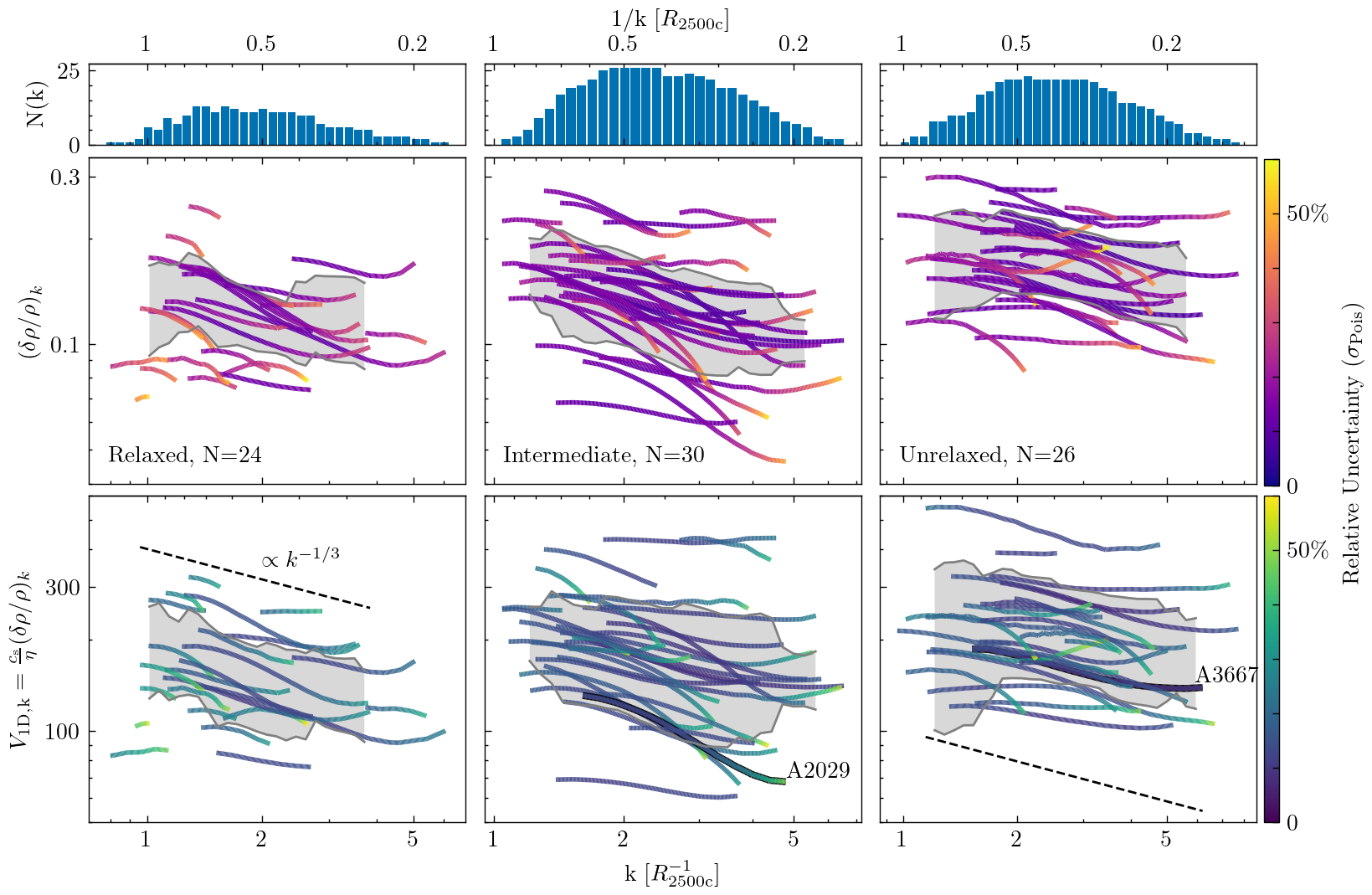
Figure 4: Middle row: Amplitude of gas density fluctuations vs. wavenumber (bottom x-axis) and length scale (top x-axis), in units of $R_{\rm 2500c}$. Each line represents one cluster, where $\left(\delta\rho/\rho\right)_{k}$ is measured within a region of radius $R_{\rm 2500c}$ (excluding cool-cores). Clusters are divided into relaxed (left), intermediate (middle), and unrelaxed (right) subsamples. Only scales largely unaffected by systematics (as discussed in Section 2.7) are shown. Line color corresponds to the measurement’s relative uncertainty, derived from $1\sigma$ Poisson uncertainties (see color scale at right). Subsample-averaged amplitudes at each length scale, plus/minus one standard deviation, are shown in grey. Bottom row: Velocity power spectra for each cluster, with equivalent notations. The Kolmogorov slope is plotted as a guide (dashed black line). Two highlighted clusters, A2029 and A3667, will be observed with XRISM during the PV phase. Top row: Number of clusters with measured $\left(\delta\rho/\rho\right)_{k}$ at each scale within each subsample. Prominent substructures are removed from the analyzed images to measure fluctuations in the bulk ICM. For the version with included substructures, see Figure 14.

We measure the scale-dependent amplitude of density fluctuations $\left(\delta\rho/\rho\right)_{k}$ and velocity power spectrum $V_{\text{1D,k}}$ in a total of 80 galaxy clusters across length scales ranging from $50$ kpc $\lesssim 1/k\lesssim 750$ kpc. Measurements from the bulk ICM (substructures excluded) are shown in Figure 4, where the sample is divided into relaxed, intermediate, and unrelaxed clusters. In this figure, we plot $\left(\delta\rho/\rho\right)_{k}$ and $V_{\text{1D,k}}$ against wavenumber/spatial scale in units of $R_{\rm 2500c}$ (bottom/top axis), where line color corresponds to the relative uncertainty $\sigma_{\left(\delta\rho/\rho\right)_{k}}/$$\left(\delta\rho/\rho\right)_{k}$ with $1\sigma$ uncertainties derived from Poisson noise as described in Section 2.7. Weighted sample averages for each morphological category are additionally shown in grey, with the shaded region corresponding to the average $\pm 1$ standard deviation. The top panels show the number of clusters with measured $\left(\delta\rho/\rho\right)_{k}$ at a given scale. Figure 14 shows equivalent measurements taken from the entire cluster, with substructures included in the calculation. We stress that the latter measurements do not represent fluctuations in the bulk ICM.

Typical amplitudes of density fluctuations in the bulk ICM are $\sim 12\pm 2$ per cent for relaxed clusters, increasing to $\sim 19\pm 5$ per cent for unrelaxed clusters when measured at $1/k=0.5$ $R_{\rm 2500c}$ (Figure 4). If substructures are included in the measurement, the level of fluctuations in relaxed clusters remains about the same, while the typical amplitude increases to $\sim 40$ per cent in unrelaxed clusters 14). One would expect to see increasing density fluctuations with merger activity, and while this is the case in the entire region (Figure 14), the effect is smaller once prominent substructures are removed.

The difference in amplitudes in the bulk ICM translates to a factor of $\gtrsim 2.5$ more ICM kinetic energy at length scales smaller than $0.5$$R_{\rm 2500c}$ in unrelaxed clusters compared to relaxed ones. This suggests that fluctuations in the bulk ICM are not strongly linked to the current merger state of the cluster. This may be because there has not been sufficient time for fluctuations in clusters with ongoing mergers to cascade to these relatively small scales. Another possibility is that fluctuations in the bulk ICM of unrelaxed clusters dissipate quickly. The opposite may also be true, that those fluctuations present in relaxed clusters are “left over” from mergers in the cluster’s more distant history.

It is additionally interesting to assess whether the density fluctuation amplitudes in relaxed vs. unrelaxed clusters belong to different populations. A Kolmogorov-Smirnov test performed at each wavenumber shows that it is difficult to distinguish between relaxed and intermediate clusters. However, density fluctuations measured in unrelaxed clusters (including substructures) are distinct from relaxed and intermediate clusters at the $p<0.05$ level between scales of $1/k\approx 0.2$ to $0.8$ $R_{\rm 2500c}$. Therefore, at these wavenumbers, the amplitude of density fluctuations could be used as an indicator of cluster dynamic state, complementing the commonly used indicators based on, e.g., the asymmetry of the X-ray surface brightness, centroid shifts, power ratios, and symmetry-peakiness alignment (e.g., Cerini et al., 2022; Yuan et al., 2022; Cui et al., 2017; Mantz et al., 2015b). Although there is some overlap between the intermediate and unrelaxed populations, $\left(\delta\rho/\rho\right)_{k}$$>20$ per cent at $1/k=0.5$$R_{\rm 2500c}$ is typically indicative of a major merger.

The scale-dependent amplitude of density fluctuations $\left(\delta\rho/\rho\right)_{k}$ can additionally be used to provide constraints on the gas clumping factor, $C$, in the ICM through a simple relation (Zhuravleva et al., 2015):

$$C-1=\left(\delta\rho/\rho\right)^{2}=\int\left(\frac{\delta\rho}{\rho}\right)_{k}^{2}\frac{dk}{k}.$$ (8)

This expression should be integrated over the entire range of wavenumbers, however, our measurements are limited to a smaller range of scales described in Section 2.7 and listed in Table LABEL:tab:clumpings. Therefore, we integrate across this range of measurable scales, interpreting this result as a lower limit on $C$, which we plot in pink in Figure 5.

To estimate the upper limit on $C$, we fit $\left(\delta\rho/\rho\right)_{k}$ to a power-law via an MCMC chain (Hogg & Foreman-Mackey, 2018) using the emcee package (Foreman-Mackey et al., 2013), and integrate this power-law from $k=1/$$R_{\rm 2500c}$ to $k=\infty$. An example of a fitted power spectrum is shown in Figure 13. The choice of $k=1/$$R_{\rm 2500c}$ is rather arbitrary, however, reasonable given the size of the considered region. These upper limits are plotted as unfilled blue markers in Figure 5, with uncertainties derived from the 84th and 16th percentile of the MCMC chain. Both lower and upper limits on the clumping factor, as well as the best-fit parameters of this power-law, i.e., the normalization of $\left(\delta\rho/\rho\right)_{k}$ at $1/k=$$R_{\rm 2500c}$ and the slope $\alpha$, are presented in Table LABEL:tab:clumpings.

The weighted-average median upper limit on the clumping factor in our sample is $C\approx 1.05\pm 0.04$. In relaxed and intermediate clusters, the average is $1.04\pm 0.02$, compared to $1.09\pm 0.04$ in unrelaxed clusters. We find reasonably good constraints on $C$ in 23 clusters, where the median lower limit on $C-1$ is within a factor of 3 of the upper limit. Namely, these clusters are Cygnus A, A1795, A2597, the Bullet cluster, A2219, A3667, A2319, A2142, A2034, A1664, A1650, MACS0717, A401, A1835, A1689, A2256, RXC1504, A3112, A2626, A2204, 4C+37.11, A2029, and A2063. Of these, most of the median upper limits are within the $1.02\lesssim C_{\text{U}}\lesssim 1.06$ range. On the high end are the Bullet cluster ($C_{\text{U}}\approx 1.12$) and MACS0717 ($C_{\text{U}}\approx 1.17$), objects with (likely) the highest clumping factors in our sample. A1914 and RBS1316 also have high $C_{\text{L}}$ but have significantly larger uncertainties. We find the lowest median upper limit on the clumping factor ($C_{\text{U}}\lesssim 1.02$) in A1650, A2199, and A2029, despite the presence of sloshing in A1650 and A2029. In comparison with other observations, our measurements are consistent with those of Eckert et al. (2015), who found $C\approx 1.05\pm 0.04$ within $0.5$$R_{\rm 500c}$ in 31 clusters. We only confirm a single cluster with $C$ outside of this range (MACS0717).

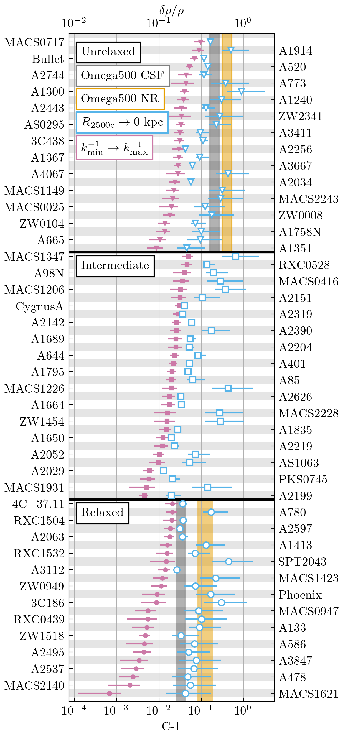
Figure 5: ICM clumping factors obtained by integrating $\left(\delta\rho/\rho\right)_{k}$ for each cluster in our sample. In pink, we integrate equation (8) from $k_{\text{min}}$ to $k_{\text{max}}$, providing a lower limit on each value. We additionally fit the observed spectrum to a power-law via MCMC and integrate from $k=1/$$R_{\rm 2500c}$ to $k=\infty$. The median values, along with upper and lower uncertainties, are presented in blue with unfilled markers. These values could be interpreted as upper limits. Clumping factors measured in the Omega500 cosmological simulations (Nagai & Lau, 2011; Zhuravleva et al., 2013) are plotted in shaded regions in their corresponding morphological categories. Grey regions show simulations where radiative processes (e.g., cooling and star formation/feedback) are included, while yellow regions show results from non-radiative simulations.

3.2 Velocity power spectra and non-thermal pressure

We convert our measured $\left(\delta\rho/\rho\right)_{k}$ into velocity power spectra using equation (5). We estimate the median sound speed in the region of interest from either our measured temperature profiles or those found in the literature, shown in Table LABEL:tab:parameters. The proportionality coefficient $\eta$ has been recently updated by Z23 (see their Figure 7) using a sample of 78 clusters from non-radiative cosmological simulations. In that work, the amplitude of density fluctuations and the Mach number of gas motions were calculated with an equivalent methodology to the one used here within a similar region. They find average values of $\eta=(\delta\rho/\rho)_{k}/\mathcal{M}_{\rm 1D,k}$ between $1/k=60$ and $300$ kpc, where the simulation resolution is not expected to affect the measurement. The $\eta$ values we use are summarized in Table 1. Resulting velocity power spectra ($V_{\text{1D,k}}$) are presented in Fig 4. Additionally, velocities in each morphological category are averaged in the same fashion as $\delta\rho/\rho$, plotted in grey regions with uncertainties as in the middle row. We see that, on average, $V_{\text{1D,k}}$ is correlated to cluster dynamical state. On a length scale of $0.5$ $R_{\rm 2500c}$, the typical $V_{\text{1D}}$ is $\sim 150$ km s^-1 for relaxed clusters, $\sim 200$ km s^-1 for intermediate clusters, and $\sim 250$ km s^-1 for unrelaxed clusters. The velocity amplitude decreases with scale, and the slope is consistent with the Kolmogorov model within the uncertainties.

To estimate the characteristic (i.e., scale-independent) velocity associated with these gas motions, we use the integrated $\delta\rho/\rho$ and calculate the one-dimensional Mach number, $\mathcal{M}_{\text{1D}}=(\delta\rho/\rho)/\eta$. This measurement can additionally be used to calculate the kinetic pressure fraction:

$$P_{\text{kin}}/(P_{\text{kin}}+P_{\text{thm}})=P_{\text{kin}}/P_{\text{tot}}=\frac{V_{\text{1D}}^{2}}{V_{\text{1D}}^{2}+kT/\mu m_{p}}=\left(1+\frac{1}{\gamma\mathcal{M}_{\text{1D}}^{2}}\right)^{-1}$$ (9)

where $P_{\text{kin}}$ is the kinetic gas pressure, $P_{\text{thm}}$ is the thermal pressure, $P_{\text{tot}}$ is the total pressure, and $V_{\text{1D}}=c_{s}\mathcal{M}_{\text{1D}}$ is the characteristic one-dimensional velocity, assuming an adiabatic index of $\gamma=5/3$. As stated previously, we do not attempt to distinguish between bulk ($V_{\text{bulk}}$) and turbulent ($V_{\text{turb}}$) gas motions. To calculate $P_{\text{kin}}/P_{\text{tot}}$, we assume that $V_{\text{1D}}\sqrt{3}=V_{\text{3D,eff}}=\sqrt{3V_{\text{turb}}^{2}+V_{\text{bulk}}^{2}}$. High-resolution X-ray spectroscopy from XRISM, NewAthena, and LEM (XRISM Science Team, 2020; Barret et al., 2020; Kraft et al., 2022) will be able to distinguish these components to confirm our measurements and this relationship.

Figure 6 shows the derived values for $\mathcal{M}_{\text{1D}}$ and $P_{\text{kin}}/P_{\text{tot}}$ for all clusters in our sample (see also Table LABEL:tab:clumpings) with equivalent notation to Figure 5. We find an average best-fit Mach number in the range of $0.18\pm 0.05$ across the entire sample, consistent with subsonic gas motions. The highest characteristic velocities we can confirm are found in MACS0717 ($V_{\text{1D}}\gtrsim 575$ km s^-1, $\mathcal{M}_{\text{1D}}\gtrsim 0.27$) and RBS1316 ($V_{\text{1D}}\gtrsim 435$ km s^-1, $\mathcal{M}_{\text{1D}}\gtrsim 0.22$). In all respects (lower limits and best-fit clumping factor/characteristic velocity), this makes RBS1316 (a.k.a RX J1347.5-1145 Johnson et al., 2012) the most disturbed cool-core cluster, indicating that significant merger effects are taking place.

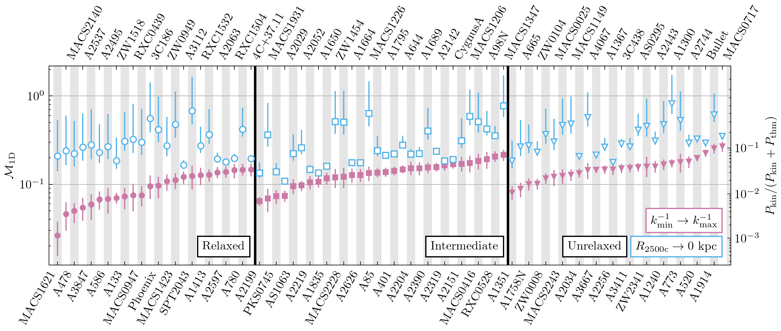
Figure 6: Characteristic one-dimensional Mach numbers (left y-axis) and kinetic pressure fractions (right y-axis) for each cluster in our sample. Notations are equivalent to Figure 5.

The lowest velocities are found in A2597, A1650, A2626, A2199, and A2029, with upper limits on $V_{\text{1D}}<200$ km s^-1, all of which are cool-core clusters. Of these, A1650, A2626, and A2029 show some evidence of mergers in the form of sloshing, while the rest are significantly relaxed. For non-cool-core clusters, the lowest velocities we confirm are A3667 and A2256, with upper limits below $V_{\text{1D}}=300$ km s^-1. Both clusters have significant substructures in the form of cold fronts (e.g., de Gasperin et al., 2022; Rajpurohit et al., 2023) and bow shocks in the case of A3667. Confirmation of the characteristic velocities in the bulk ICM with direct observation should carefully exclude emission from these prominent substructures.

Measuring non-thermal pressure support is important for cosmology based on hydrostatic cluster mass measurements (e.g., Allen et al., 2008; Vikhlinin et al., 2009; Mantz et al., 2016a; Clerc & Finoguenov, 2023). We place upper limits (denoted with the lower index $U$) on the fraction of kinetic pressure in the bulk ICM at $\left(P_{\text{kin}}/P_{\text{tot}}\right)_{U}<10$ per cent in a total of 22 clusters within the $R_{\rm 2500c}$ region, with $\left(P_{\text{kin}}/P_{\text{tot}}\right)_{U}<5$ per cent in A2219, A1650, PKS0745, A1835, A2199, and A2029. A2029 has the lowest non-thermal pressure contribution of $\sim 1.9$ per cent. Most clusters among these 22 are classified as relaxed or intermediate. Three clusters in this subsample, however, are unrelaxed clusters: A3667, A2034, and A2256, each with $\left(P_{\text{kin}}/P_{\text{tot}}\right)_{U}<8$ per cent in the bulk ICM despite significant ongoing merger processes. For these clusters, it is important to note that the measured kinetic pressure in the bulk ICM is unlikely to reflect the total kinetic pressure in the entire cluster, contributions from merger-driven substructures could be significant. In our sample, the weighted-average best-fit upper limit for the kinetic pressure fraction ($\langle P_{\text{kin}}/P_{\text{tot}}\rangle_{U}$) are approximately $6\pm 2$ per cent for relaxed clusters, $4\pm 2$ per cent for intermediate clusters, and $7\pm 4$ per cent for unrelaxed clusters. Note that intermediate and unrelaxed clusters will likely have significant kinetic pressure associated with discrete substructures, which are removed from these measurements.

Recent constraints have been placed on the kinetic pressure fraction in a similar region of the Perseus (de Vries et al., 2023) and Ophiuchus (Gatuzz et al., 2023) clusters, finding $6\lesssim P_{\text{kin}}/P_{\text{tot}}\lesssim 13$ per cent and $P_{\text{kin}}/P_{\text{tot}}\lesssim 18$ per cent, respectively. All of our clusters agree with the latter measurement, and all but 12, with upper limits on $P_{\text{kin}}/P_{\text{tot}}<6$ per cent, agree with the former.

4 Discussion

4.1 Comparisons with cosmological simulations

4.1.1 Multi-scale density fluctuations

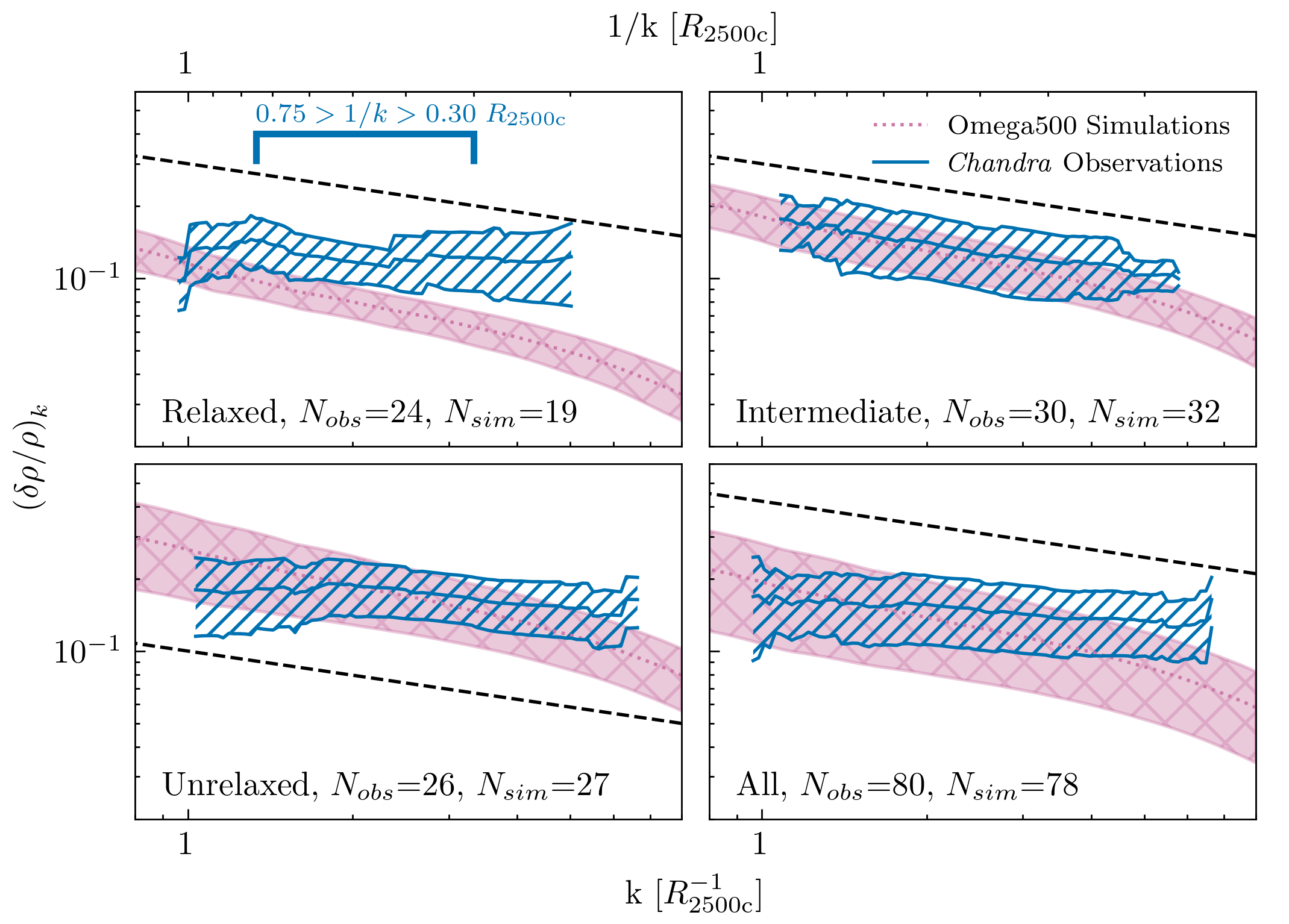
Figure 7: Sample-averaged $\left(\delta\rho/\rho\right)_{k}$ measured in the bulk ICM of relaxed, intermediate, unrelaxed, and all clusters. Observational measurements from this work are plotted in blue, with $1\sigma$ uncertainties in the hatched regions. Measurements from Omega500 cosmological simulations (for power spectra, see Zhuravleva et al., 2023) are plotted in pink. The blue bracket represents length scales where we confirm a divergence between observed and simulated measurements in relaxed systems. Black dashed lines represented a $k^{1/3}$ power-law relationship for guidance.

Scale-dependent amplitudes of density (or any other characteristic) fluctuations can be used as sensitive probes of multi-scale, non-linear physics and sub-grid prescriptions in numerical simulations. An equivalent method of measuring density fluctuations has been recently applied to a representative sample of 78 galaxy clusters (Zhuravleva et al., 2023) from the Omega500 cosmological simulations (Nagai et al., 2007a, b; Nelson et al., 2014b). Similar to our work, the authors split the simulated clusters into relaxed, intermediate, and unrelaxed systems and considered fluctuations in the bulk ICM (i.e., removing prominent substructures) within a similar region ($r\leq 0.5R_{500c}$). The authors considered fluctuations in simulations with non-radiative physics, which apply to the regions considered in our work (i.e., beyond cool-cores and least affected by cooling and feedback processes).

Figure 7 shows the average amplitude of density fluctuations, with one standard deviation as uncertainties, in simulated and observed clusters in pink and blue, respectively. In clusters with evidence of mergers (the intermediate and unrelaxed subsamples), observed and simulated amplitudes of density fluctuations are consistent across all scales. In relaxed clusters, however, the amplitudes diverge on small scales, reaching a factor $\gtrsim 2$ difference between the mean values at $1/k\lesssim 0.3$$R_{\rm 2500c}$ (typically $\sim$ 120 kpc). Performing a Kolmogorov-Smirnov test at each length scale, we confirm that the distribution of density fluctuations observed in our relaxed cluster sample are distinct from the simulations between $1/k=0.75$ and $0.3$ $R_{\rm 2500c}$ ($\sim 300-120$ kpc, the dark blue bracket in the top-left panel), with the probability of the two samples being derived from the same distribution being $<0.05$ at these scales. On scales smaller than $1/k\sim 0.3$$R_{\rm 2500c}$, we observe a similar tension, however, the number of clusters where we could probe these scales is small, less than 10. If the observational and simulated measurements are compared with wavenumber in kpc^-1 (instead of re-scaling with $R_{\rm 2500c}$), we observe this tension in relaxed clusters between $\sim$120 and 300 kpc.

We checked whether observational biases could cause this tension. Fluctuations in five clusters in the relaxed sample (A2537, A3847, A478, MACS1621 and MACS2140, see Figure 4) are measured on large scales ($1/k\gtrsim 0.6$$R_{\rm 2500c}$) with $\left(\delta\rho/\rho\right)_{k}$$<10$ per cent. Extrapolating these amplitudes to smaller scales gives very small amplitudes of fluctuations, which are difficult to measure reliably given Poisson noise, background, and contribution from unresolved point sources. However, if these spectra were observed on small scales, they could reduce the average amplitude of observed density fluctuations, bringing it closer to the simulation average. To examine this potential bias, we extrapolate the power spectra in these five clusters across smaller scales, fitting the observed spectra with a power-law as described in Section 3.1, and assuming the slope of $\left(\delta\rho/\rho\right)_{k}$ extends across the entire range of length scales. With these extended power spectra, we reanalyze the tension in relaxed clusters. While the distributions of $\left(\delta\rho/\rho\right)_{k}$ in the observed and simulated subsamples become compatible at small scales (where we initially observed less than 10 clusters), the tension remains strong between $0.3\lesssim 1/k\lesssim 0.75$ $R_{\rm 2500c}$. This conclusion remains if we assume a fixed Kolmogorov slope of $-1/3$, or if the extrapolation across all scales is applied to every cluster in the sample.

Our measured power spectra could also be affected by unresolved point sources or, e.g., additional variations on the detector, especially on small scales. To check the potential effect of these, we take a more conservative value for the maximum wavenumber measured reliably in each cluster by only considering wavenumbers where we do not observe any flattening of the $\left(\delta\rho/\rho\right)_{k}$ slope. We find that even with reduced limits, the divergence between observation and simulations remains across most of the range. We additionally compare the observed spectrum when no correction for the Chandra PSF (see Section 2.7) is applied, and find no change in the length scales where the divergence is observed.

One could expect that density fluctuations also correlate positively with redshift since the merger rate increases with redshift according to hierarchical structure formation. Our sample covers a range of redshifts up to $z\sim 1$, while the Omega500 clusters were analyzed at $z=0$. To check whether the observed tension could be caused by this redshift evolution of $\delta\rho/\rho$, we recalculate the Kolmogorov-Smirnov test excluding high-redshift systems, and conclude that the redshift evolution did not significantly affect the result.

Finally, we check if our morphological classification of galaxy clusters has any effect on the observed tension between the observations and simulations. We identify clusters that may be on the boundary between morphological categories and recalculate the averaged spectra and K-S test when the morphological classification is randomly varied between categories for each boundary object. We find that the tension is strong even if the classification is varied or if these boundary objects are removed from the sample entirely. To conclude, the tension appears real and is stable to observational systematics. Simply put, we do not observe clusters with the low-amplitudes fluctuations that are common in simulations at scales of $1/k\lesssim 0.75$$R_{\rm 2500c}$.

Note, the displayed scales from simulations are not expected to be affected by the resolution of simulations, which becomes evident on length scales below $\sim 60$ kpc ($\lesssim 0.15$$R_{\rm 2500c}$, Z23, see their Section 4.2). Moreover, the divergence in averaged $\left(\delta\rho/\rho\right)_{k}$ is only observed in relaxed clusters and not in the intermediate or unrelaxed subsamples. Therefore, this divergence in relaxed clusters is unlikely to be driven primarily by numerical viscosity.

As the factor of $\sim 1.5$ to $2.5$ difference between the amplitude of density fluctuations on length scales smaller than $0.75$$R_{\rm 2500c}$ in relaxed clusters cannot be explained by known observational/instrumental effects and is unlikely to be caused by the resolution of cosmological simulations, it could be attributed to missing physics in the simulations we consider. Radiative processes (e.g., gas cooling), AGN feedback, galactic outflows, and magnetic fields could all increase $\left(\delta\rho/\rho\right)_{k}$ at these scales. Fluctuations in relaxed clusters appear to be more sensitive to these physics compared to perturbed systems, in which ongoing mergers continuously “stir” the ICM and contribute significantly to the observed amplitude of density fluctuations. While it is straightforward to extend the analysis of density fluctuations to other simulations and simulation runs that include these additional physics, it is beyond the scope of this work. The observed tension also means that relaxed clusters should be selected for testing additional physics implemented in simulations, especially multi-scale physics, against observations.

With these measurements, we cannot distinguish between which of the above processes is the primary driver of the observed divergence. The central AGN mostly affects gas dynamics within the cool-core and is not influential in the regions considered, however AGN and galaxy-scale outflows originating from other cluster galaxies could affect density fluctuations in relaxed clusters more strongly than in merging ones. Additionally, while cooling times in the regions considered are greater than the Hubble time, radiative physics could still affect $\left(\delta\rho/\rho\right)_{k}$ in simulations (e.g., by creating clumpy structures, see Section 4.1.2 below).

Finally, the fact that relaxed clusters appear “smoother” in simulations compared to observations could have consequences for cluster cosmology predictions based on hydrostatic mass measurements (e.g., Mantz et al., 2015a; Vikhlinin et al., 2009; Pratt et al., 2019). Namely, the predicted contribution of non-thermal pressure from simulations could be underestimated (e.g., Lau et al., 2012; Nelson et al., 2014b). We leave the quantitative exploration of this issue for future works.

4.1.2 Clumping factor and non-thermal pressure

It is interesting to compare the estimated ICM clumping factor shown in Figure 5 with predictions from numerical simulations. In earlier works based on Omega500 simulations, Nagai & Lau (2011) found that $1.03<C<1.04$ in relaxed clusters and $1.16<C<1.26$ in unrelaxed ones within $R_{\rm 2500c}$ when radiative processes (e.g., cooling, star formation/feedback, hereafter CSF) are included (see also Zhuravleva et al., 2013). The non-radiative runs predict a higher level of clumpiness, $\sim 1.14$ ($1.48$) for relaxed (unrelaxed) systems, see gray and yellow regions in Figure 5. More recently, Angelinelli et al. (2021) found $1.05<C<1.15$ in a sample of clusters from the non-radiative Itasca cluster sample (Vazza et al., 2017). Our measurements are broadly consistent with these values. Specifically, we find that nearly all relaxed and two-thirds of unrelaxed clusters in our sample are consistent with the Omega500 CSF predictions. The remaining third of unrelaxed clusters have upper limits lower than predicted in these simulations. Clumping in non-radiative runs in Omega500 is systematically higher and consistent with $\sim 70$ per cent of the relaxed and $\sim 45$ per cent of unrelaxed clusters from our sample. As for the Itasca simulations, we find that 15 out of 80 clusters in our sample have clumping factors constrained below $1.05$, the rest are consistent with the predicted range.

The non-thermal pressure fraction, shown in Figure 6, has also been measured in several cosmological simulations. Battaglia et al. (2012); Nelson et al. (2014b); Shi et al. (2015) find that, broadly, $P_{\text{kin}}/P_{\text{tot}}$ ranges between $\sim 5$ per cent and $25$ per cent in the bulk ICM within $\sim$$R_{\rm 2500c}$. In our sample, 76 clusters (95 per cent of our sample) could fall within this range; among these, 6 clusters with the tightest constraints: A2744, the Bullet cluster, A520, MACS0717, 4C+37.11, and RXC0528. The 4 clusters with kinetic pressure fractions below this range, those mentioned in Section 3.2, have exceptionally low $P_{\text{kin}}/P_{\text{tot}}$. Our measurements are, therefore, consistent with these simulations.

4.2 ICM plasma physics

4.2.1 Turbulent re-acceleration of cosmic rays

Other than the X-ray thermal emission, the ICM also exhibits non-thermal synchrotron emission that is bright in radio (e.g., van Weeren et al., 2019). In particular, volume-filling radio halos are thought to be powered by turbulent re-acceleration of seed relativistic cosmic ray electrons (CRe) (e.g., Petrosian & Bykov, 2008; Brunetti & Lazarian, 2011; Brunetti, 2016; Brunetti et al., 2017). From this model, one may expect a correlation between the observed radio power ($P_{\text{1.4 GHz}}$) and ICM turbulence (or kinetic energy) (e.g., Bonafede et al., 2018), likely with significant scatter due to cluster-to-cluster variation of the seed CRe population (Nishiwaki & Asano, 2022).

This relationship has been previously investigated (with mixed results) by Eckert et al. (2017) and Zhang et al. (2022). Eckert et al. (2017) found a strong correlation between the $V_{\text{1D,k}}$ (at $1/k=660$ kpc) and $P_{\text{1.4 GHz}}$, finding a Pearson correlation coefficient of $r_{V:P}\approx 0.8$ in a sample of 25 radio halo detections (their sample also included 26 clusters with upper limits on $P_{\text{1.4 GHz}}$). Zhang et al. (2022), however, were unable to find any significant correlation between the same measurements in a sample of 11 halos, with $r_{V:P}\approx 0.4$ ($1/k\approx 400$ kpc). Both studies inferred velocities indirectly through a similar method used in this work. The correlation has also been explored within individual clusters. Bonafede et al. (2018) found kinetic energy in MACS0717 $\sim 30$ per cent higher in the region with strong radio emission compared to the radio-quiet region.

In our sample, 22 clusters have detected radio halos at 1.4 GHz, in addition to 5 with upper limits (see Table LABEL:tab:parameters for details and references). It is interesting to check the radio power - turbulence relation, especially since we are probing smaller scales that are least affected by the choice of underlying model, merging substructures, and large-scale asymmetries (Section 2.5). At multiple length scales, we compare the characteristic velocity to radio power in these 22 clusters, calculating $r_{V:P}$ at each scale. Representative distributions of $V_{\text{1D,k}}$ and $P_{\text{1.4 GHz}}$ are plotted in Figure 8, where velocity is measured at 0.3 $R_{\rm 2500c}$ (blue circles) and 0.6 $R_{\rm 2500c}$ (pink squares). Galaxy clusters with radio halo upper limits are also plotted as unfilled points.

To calculate uncertainties on $r_{V:P}$, we assume the measurement uncertainties on $V_{\text{1D,k}}$ and $P_{\text{1.4 GHz}}$ are approximately Gaussian and randomly sample this distribution, finding the standard deviation on this randomized correlation coefficient. Additionally, we estimate the sample variance of $r_{V:P}$ via a bootstrap, combining these uncertainties in quadrature. The latter source of uncertainty is much more significant at all scales.

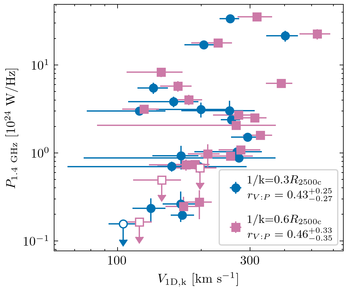
Figure 8: Radio halo power at 1.4 GHz (see Table LABEL:tab:parameters for references) versus characteristic velocity $V_{\text{1D,k}}$ at $1/k=0.6$ (blue circles) and $0.3$ $R_{\rm 2500c}$ (pink squares). Unfilled squares/circles indicate upper limits on radio halo power. The Pearson correlation coefficients $r_{V:P}$ at the two different length scales are shown in legends. Uncertainties on $r_{V:P}$ are calculated via a bootstrap and by randomly sampling measurement uncertainties on $V_{\text{1D,k}}$ and $P_{\text{1.4 GHz}}$. For clusters with $V_{\text{1D,k}}$ measured at both scales, paired pink and blue points are offset for visual clarity.

Across all length scales where velocities are measurable in most clusters, we find a mostly scale-independent correlation coefficient of $r_{V:P}\approx 0.45\pm 0.3$. This correlation is significantly weaker than that found by Eckert et al. (2017), and similar to that of Zhang et al. (2022). Given our larger sample size than the latter work, we can confirm a weak positive correlation at the $p<0.05$ level between scales of $1/k\approx 0.9$ to $0.3$ $R_{\rm 2500c}$ (see Figure 9).

We stress that though we see a weak positive correlation in our full sample, this correlation is driven by a single outlier cluster, MACS0717, which has the highest characteristic velocity in our sample at the scales we consider here, and the second highest radio power. Removing MACS0717 from the calculation results in a correlation coefficient consistent with $r_{V:P}=0$ at all wavenumbers. A similar but less drastic reduction in $r_{V:P}$ is seen when the Bullet cluster is removed from the sample. These two clusters are present in the Eckert et al. (2017) sample, but not in that of Zhang et al. (2022), suggesting that the strong correlation found in the former work may also be significantly driven by these same clusters. Confirmation of this correlation, therefore, requires a larger sample of radio halo and direct velocity measurements.

Given the large uncertainties on $r_{V:P}$, a strong correlation cannot be excluded. To further investigate, we attempt to fit the $V_{\text{1D,k}}$—$P_{\text{1.4 GHz}}$ distribution to a power-law relationship. Using the Bayesian MCMC routine LinMix (Kelly, 2007), which includes clusters with upper limits on $P_{\text{1.4 GHz}}$, we find that the correlation between these variables is not strong enough to recover a best-fit slope. The slope varies significantly, between $\sim 2$ and $\sim 10$, depending on the numerical method used. This is also the case when traditional MCMC maximum-likelihood fitting and orthogonal distance regression are used.

It is well-established that $P_{\text{1.4 GHz}}$ strongly correlates with cluster mass (e.g., Cassano et al., 2023, 2013). This correlation could contribute to the radio power - velocity correlation. Therefore, besides radio power, we consider $P_{\text{1.4 GHz}}/M_{\text{2500c}}$, which is a proxy for the efficiency of radio emission generation. This characteristic is compared to the turbulent energy dissipation rate $\epsilon_{\text{K}}\propto V_{\text{1D,k}}^{3}k$ and $\mathcal{M}_{\text{1D,k}}^{2}$, which traces the ratio of kinetic to thermal energy in the ICM. For each of these cases, we calculate the Pearson correlation coefficient across a range of length scales from $1$ to $0.15$ $R_{\rm 2500c}$, shown in the lower panel of Figure 9. In the upper panel of this figure, we plot the number of clusters in which $V_{\text{1D,k}}$ is observable at each scale. We additionally test other combinations of these variables, which do not change our conclusions.

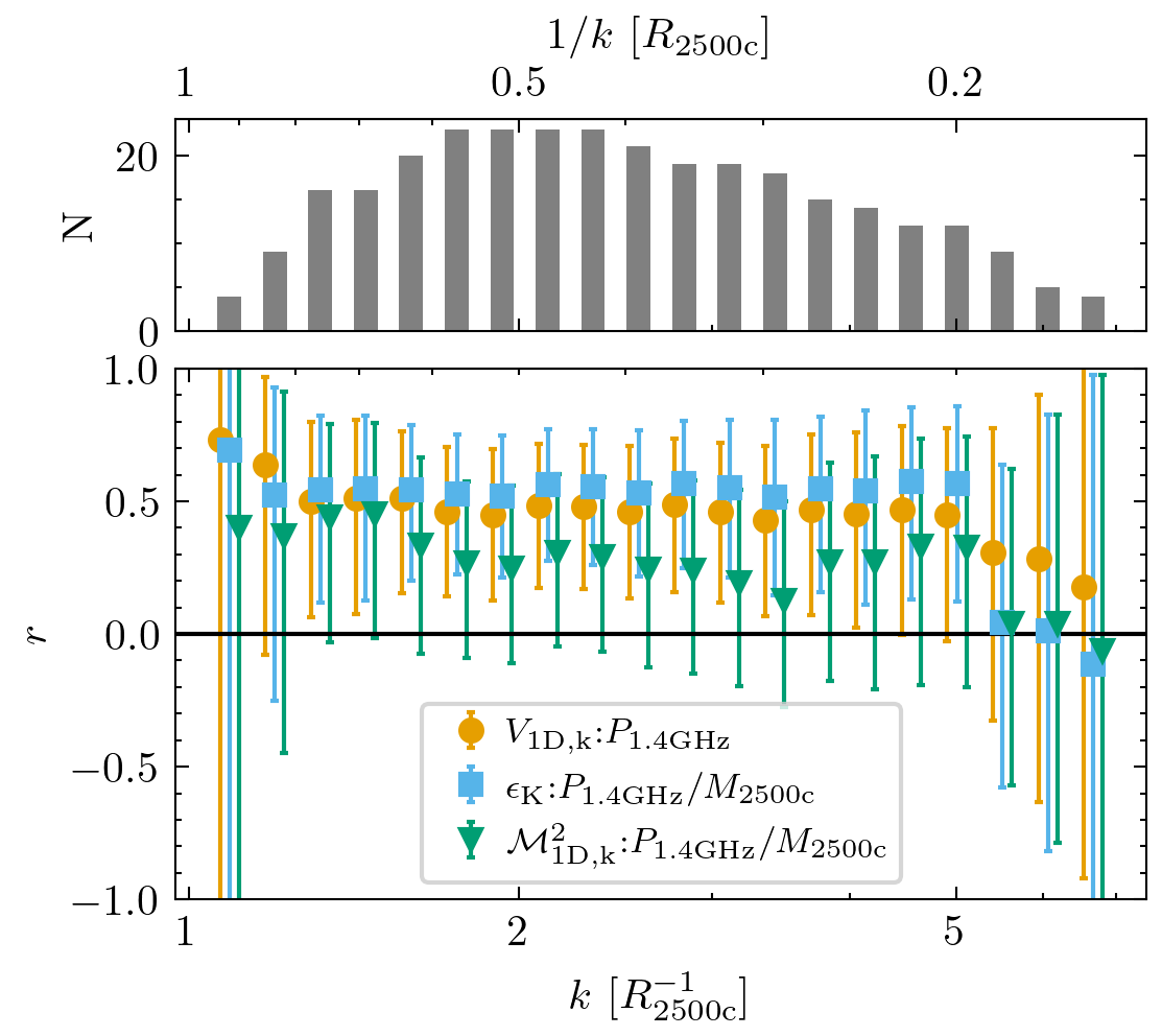
Figure 9: Pearson correlation coefficient $r$, with $1\sigma$ uncertainties, as a function of wavenumber/scale, comparing $V_{\text{1D,k}}$ to $P_{\text{1.4 GHz}}$ (orange), $\epsilon_{\text{K}}$ to $P_{\text{1.4 GHz}}/M_{\text{2500c}}$ (blue), and $\mathcal{M}_{\text{1D,k}}^{2}$ to $P_{\text{1.4 GHz}}/M_{\text{2500c}}$ (green). Uncertainties on $r$ are calculated via a bootstrap and by randomly sampling measurement uncertainties on $V_{\text{1D,k}}$ and $P_{\text{1.4 GHz}}$. $r=0$ is plotted as a solid black line. The number of clusters where $V_{\text{1D,k}}$ is measurable at each scale is plotted in the top panel. The p-value of each Pearson test is plotted in the bottom panel, with $p=0.05$ plotted as a dashed black line.

The strongest correlation we found is when comparing radio emission efficiency to the turbulent dissipation rate, with $r_{\epsilon:P/M}\approx 0.55\pm 0.3$, significant at the $p<0.05$ level at length scales larger than $0.25$ $R_{\rm 2500c}$. This correlation is also significantly driven by outlier clusters, as described above. The comparison of $P_{\text{1.4 GHz}}/M_{\text{2500c}}$ to $\mathcal{M}_{\text{1D,k}}^{2}$ is consistent with no correlation at all scales.

Further investigation of the relationship between ICM gas motions and non-thermal emission could be improved by larger samples of radio halo detections and velocity measurements, including direct velocity measurements with XRISM that will soon become available. We note that $P_{\text{1.4 GHz}}$ is measured across the entire extent of the radio halo (with typical radii of $\sim 1$ Mpc), while our characteristic velocities are measured within $R_{\rm 2500c}$ ($\sim 500$ kpc). The effect of this mismatch is expected to be small, as typically $\sim 90$ per cent of the total emission from radio halos is found within $R_{\rm 2500c}$ (Botteon et al., 2022). Additionally, the radio power measured at 1.4 GHz does not reflect the total luminosity of the halo, as there is evidence for variation in spectral slope between halos (van Weeren et al., 2019). Moreover, in some cases, significant areas around prominent substructures are removed. Thus, the comparison between our X-ray measurements and radio powers found in the literature is not one-to-one and could be improved in future works.

If substructures are included in the estimations of $V_{\text{1D,k}}$, the strength of all correlations increases on length scales smaller than $\sim 0.8$$R_{\rm 2500c}$. $r_{V:P}$ and $r_{\epsilon:P/M}$ both rise to $\sim 0.7\pm 0.3$. Thus, we find that improper treatment of X-ray substructures may lead to spurious correlations that do not reflect the state of the bulk ICM.

4.2.2 Constraints on effective viscosity

Threaded by a weak, likely tangled $\sim$ few $\mu G$ magnetic field (e.g., Carilli & Taylor, 2002), the ICM is prone to the firehose and mirror plasma instabilities. These produce fluctuations, which can scatter particles, increasing their effective collisional rate and, therefore, decreasing the effective viscosity of the ICM (Schekochihin & Cowley, 2006). At the same time, the gyroradius of ions is many orders of magnitude smaller than the typical Coulomb mean free path. Therefore, particles are confined to magnetic field lines, making the transport of heat and momentum anisotropic with respect to the local magnetic field (Kunz et al., 2011).

Observations of prominent structures within the ICM support these predictions. For instance, the width of interfaces between two gas phases in cold fronts is typically narrower than the mean free path of particles, indicating suppressed diffusion, conduction and mixing across the interface (e.g., Markevitch & Vikhlinin, 2007; Werner et al., 2016; Zuhone & Roediger, 2016). The presence of Kelvin-Helmholtz instabilities in cold fronts (e.g., Werner et al., 2016; Ichinohe et al., 2017; Su et al., 2017; Hu et al., 2021) and the morphology of stripped tails of infalling galaxies and groups (e.g., Kraft et al., 2017) also support suppressed effective viscosity, typically $\lesssim 5$ per cent, with respect to the isotropic Spitzer level ($\nu_{0}$, Spitzer, 1962). Probing the effective viscosity in the bulk ICM has recently become possible through the measurements of density fluctuation power spectra in the Coma cluster on scales comparable to the Coulomb mean free path ($\lambda_{\text{mfp}}$). The shape of the spectra indicated $\nu_{\text{eff}}/\nu_{0}\lesssim 10$ per cent regardless of the level of thermal conduction (Zhuravleva et al., 2019). With our measurements, it is possible to expand the latter analysis to a sample of 16 clusters, for which $\left(\delta\rho/\rho\right)_{k}$ are measured across a broad range of scales close to the mean free path.

Using deprojected profiles of ICM temperature and density, we calculate radial profiles of $\nu_{0}$ (see Sarazin, 1988, for details). From our measurements of the scale-dependent characteristic velocity and under the assumption of Kolmogorov turbulence, we additionally find the turbulent energy dissipation rate ($\epsilon_{K}$) as $\epsilon_{K}=2\pi\left(3C_{K}/2\right)^{3/2}V_{\text{1D,k}}^{3}k$, where $C_{K}\approx 1.65$ is the Kolmogorov constant (Zhuravleva et al., 2014a). Given $\nu_{0}$ and $\epsilon_{K}$ we find the median Kolmogorov microscale $\eta_{K}=\left(\nu_{0}^{3}/\epsilon_{K}\right)^{1/4}$ within our region of interest. The values of $\eta_{K}$ we find are listed in Table LABEL:tab:parameters.

Using these characteristics, we rescale power spectra of all clusters in our subsample, see Figure 10 (purple-orange curves), and obtain the weighted mean value (the gray region). We also plot the earlier-measured power spectra in the Coma cluster (gray hatched regions). For comparison with simulations, the equivalent spectra of passive scalars from direct numerical simulations (DNS) of hydrodynamic turbulence (Gauding et al., 2014) are also plotted with different colors. The passive scalar is characterized by the thermal Prandtl number $Pr$, the ratio of kinematic viscosity and thermal conductivity. We use the DNS simulations for $Pr=1$, $0.25$ and $0.11$. We note that the Prandtl number of density fluctuations in the ICM is generally unknown, however it is expected to be less than unity (Kunz et al., 2022), thus we vary $Pr$ in this range. The DNS spectra predict that the passive scalar spectrum should exponentially decline/steepen on scales probed with our observations. This steepening is not observed in any measurement of $\left(\delta\rho/\rho\right)_{k}$ from this subsample, confirming earlier results based on the Coma cluster and suggesting that suppressed transport in the bulk of the gas is a general property of the ICM.

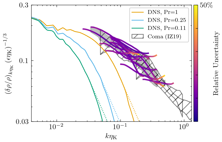
Figure 10: Observed rescaled $\left(\delta\rho/\rho\right)_{k\eta_{K}}$ in the 16 clusters in which we constrain effective viscosity. Notations are equivalent to Figure 4, with the sample-averaged values $\pm 1\sigma$ uncertainties shown with the grey region. The equivalent passive scalar power spectra from DNS simulations of hydrodynamic turbulence for three thermal Prandtl numbers are shown in solid lines. The dotted lines show how the exponential cutoff of the DNS spectra would be modified if the $\Delta$-variance method of calculating power spectra was used. Hatched regions show upper and lower limits on rescaled $\left(\delta\rho/\rho\right)_{k}$ taken from the central and outer regions of the Coma cluster (Zhuravleva et al., 2019), for comparison. The slope of the observed spectrum is shallower at the equivalent $k\eta_{\text{K}}$ than any of the DNS spectra, suggesting a suppressed effective viscosity in the ICM.

Following the Coma analysis, we can use these spectra to place upper limits on $\nu_{\text{eff}}$. Suppressing $\nu_{\text{eff}}$ lowers $\eta_{K}$, essentially moving the DNS spectra to higher wavenumbers ($k\eta_{\text{K}}$) such that the slope of measured $\left(\delta\rho/\rho\right)_{k}$ eventually matches the slope of the DNS spectra. We use an MCMC chain with the Kolmogorov microscale and the normalization as free parameters to find the highest value of $\nu_{\text{eff}}/\nu_{0}$ that provides a reasonable fit to the observed spectrum. These upper limits are presented for each object as green arrows in Figure 11. Additionally, we find the weighted average and standard deviation of $\left(\delta\rho/\rho\right)_{k\eta_{\text{K}}}\left(\epsilon_{\text{K}}\eta_{\text{K}}\right)^{-1/3}$ in this subsample and find an upper limit for the average spectrum, which is plotted as a dashed black line in the same figure.

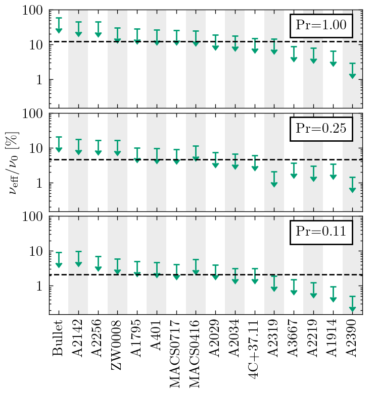
Figure 11: Upper limits on effective viscosity suppression, $\nu_{\text{eff}}/\nu_{0}$, relative to a Spitzer value in a subsample of 16 galaxy clusters for different thermal Prandtl numbers. Sample-averaged upper limits are plotted as dashed black lines.

We do not find any clusters in this subsample that are consistent with Spitzer-level effective viscosity. With $Pr=1.0$, viscosity is suppressed by at least a factor of 2 in nearly all clusters. With $Pr=0.11$, the suppression is at least a factor of 10 in all clusters, and a factor of 20 in all but 3 clusters. On average, the effective viscosity $\nu_{\text{eff}}/\nu_{0}$ is below 13 per cent in the case of $Pr=1.0$, $\lesssim 5$ per cent for $Pr=0.25$, and $\lesssim 2$ per cent for $Pr=0.11$. The strongest effective viscosity suppression in the sample is found in A2390, with $\nu_{\text{eff}}/\nu_{0}\lesssim 3$ per cent for all Prandtl numbers we considered here. This demonstrates that, indeed, magnetic fields modify the behavior of particles in the ICM, suppressing transport properties of the bulk of the gas, and that this is a general property of ICM plasmas.

We note that the $\Delta$-variance method is designed to measure smooth, power-law power spectra. The dotted lines in Figure 10 show how exponential cutoffs are modified by the $\Delta$-variance method (for details, see Arevalo et al., 2012; Zhuravleva et al., 2019). Accounting for this correction does not affect the viscosity constraints shown in Figure 11.

Additionally, we note that we use the median measurement of the Kolmogorov microscale. Within the regions we consider in this work, $\eta_{\text{K}}$ typically varies by a factor of $\sim 2$, which could increase the upper limit on $\nu_{\text{eff}}/\nu_{0}$. If the minimum value of $\eta_{\text{K}}$ is used instead of the median, we still detect effective viscosity suppression in all systems except the Bullet cluster and A2142 (for the $Pr=1.0$ case). A2390 has the largest variance, where our upper limit on $\nu_{\text{eff}}/\nu_{0}$ increases by a factor of $\sim 4.5$ if the minimum value of $\eta_{\text{K}}$ is used instead of the median, however $\nu_{\text{eff}}/\nu_{0}$ is still $\lesssim 13$ per cent for $Pr=1.0$, even in this conservative limit.

5 Conclusions

By measuring the power spectra of X-ray surface brightness fluctuations in a sample of 80 galaxy clusters observed with Chandra, we obtain the amplitude of density fluctuations and, indirectly, characteristic velocities in cluster regions dominated by merger activity, i.e., outside the cool-cores and within the $R_{\rm 2500c}$ radius. Each cluster is treated individually to ensure robust measurements at the wavenumbers/length scales we present. Observational effects (e.g., Poisson noise, PSF effects, contribution of unresolved point sources) and systematic uncertainties induced by the choice of unperturbed model and cluster substructures are carefully tested and removed. Galaxy clusters are categorized into relaxed, intermediate, and unrelaxed merger states based on their X-ray morphology and a literature review. Scale-dependent amplitudes of density fluctuations, $\left(\delta\rho/\rho\right)_{k}$, are averaged within each morphological category. Our main findings are summarized below.

• We observe a mild increase in $\left(\delta\rho/\rho\right)_{k}$ measured in the bulk ICM from relaxed to unrelaxed clusters. E.g., at $1/k=0.5$$R_{\rm 2500c}$, $\left(\delta\rho/\rho\right)_{k}$ $\sim 12\pm 2$ per cent in relaxed clusters and $\sim 19\pm 5$ per cent in unrelaxed ones. This suggests that fluctuations in the bulk ICM are not strongly dependent on recent merger activity.

• When prominent substructures are included in the measurement, density fluctuations in merging clusters ($\sim 40$ per cent at $1/k=0.5$$R_{\rm 2500c}$) are significantly higher than in relaxed clusters ($\sim 12$ per cent). Between length scales of $\sim 0.2$ to $0.8$$R_{\rm 2500c}$ ($\sim 80$ to $450$ kpc), $\left(\delta\rho/\rho\right)_{k}$ measured including substructures could be used as an indicator of cluster dynamic state, complementing other commonly-used methods.

• Power spectra of density fluctuations measured on scales from $1/k\sim 1$ to $0.2$$R_{\rm 2500c}$ in intermediate and unrelaxed clusters are in good agreement with theoretical predictions from cosmological simulations considered here.

• On length scales smaller than $\sim 0.75$$R_{\rm 2500c}$, density fluctuations measured in relaxed clusters are systematically higher by a maximum factor of $\sim 2.5$ compared to similar clusters in cosmological simulations. The effects of observational biases and numerical viscosity are likely minimal on these scales, as discussed in Section 4.1.1. The tension could be due to missing radiative and feedback physics in considered simulations. Fluctuations in relaxed clusters are most sensitive to these physics compared to merging clusters, in which the amplitude of fluctuations is likely dominated by ongoing or recent mergers. For this reason, relaxed clusters are the most useful probes for additional, multi-scale physics in simulations compared to clusters in other dynamic states.

• Estimated from power spectra of density fluctuations, clumping factors typically vary between $1.01\lesssim C\lesssim 1.10$ within the $R_{\rm 2500c}$ region in our sample, with a few outliers (the Bullet and MACS0717 clusters). The measured clumping factors are broadly consistent with predictions from cosmological simulations, and in good agreement with other existing measurements within a similar region.

• Using a statistical relation between the amplitude of density fluctuations and velocity (with a recently-updated proportionality coefficient for clusters in different dynamical states), we find that the sample-average one-dimensional velocities are $\sim 150$ ($250$) km s^-1 at $1/k=0.5$$R_{\rm 2500c}$ for relaxed (unrelaxed) clusters. Within the uncertainties, the average power spectrum slope is consistent with a Kolmogorov cascade, although the uncertainties are large.

• Characteristic velocities (scale-independent) in the range of a few 100 km s^-1 are found in essentially all clusters. The lowest velocities, $V_{\text{1D}}<200$ km s^-1, are found in A2597, A1650, A2626, A2199, and A2029. The highest velocities, $V_{\text{1D}}>350$ km s^-1, are found in the Bullet cluster, A1916, RBS1316 and MACS0717. These velocities await confirmation via direct observation by XRISM.

• We confirm kinetic pressure fractions in the bulk ICM of $\lesssim 10$ per cent in 22 clusters, and $\lesssim 5$ per cent in 6 of these: A2219, A1650, PKS0745, A1835, A2199, and A2029. The lowest is found in A2029. Note these values likely do not represent the total kinetic pressure support unless the cluster is unaffected by merging substructures (relevant to most relaxed clusters in our sample). These values of non-thermal pressure support are consistent with predictions from cosmological simulations.

• Using a subsample of galaxy clusters that host extended radio halos, we measure a weak positive correlation between characteristic velocity and radio power between length scales of $0.9\gtrsim 1/k\gtrsim 0.3$$R_{\rm 2500c}$, consistent with Zhang et al. (2022) but weaker than Eckert et al. (2017). We additionally test correlations between the “radio emission efficiency” ($P_{\text{1.4 GHz}}/M_{\text{2500c}}$), turbulent energy dissipation rate ($\epsilon_{K}$), and the ratio of kinetic to thermal energy ($\mathcal{M}_{\text{1D,k}}^{2}$). The strongest correlation we find is between $\epsilon_{K}$ and radio emission efficiency, with the Pearson $r_{\epsilon:P/M}\approx 0.55\pm 0.3$.

• While these correlations are somewhat significant in the full sample, it is important to note that they are driven by a few outlier clusters. Removing the Bullet cluster or MACS0717 from the sample significantly reduces the correlation, such that the Pearson test is consistent with zero. Additionally, the results can be significantly affected by the inclusion/exclusion of substructures and the choice of underlying model. This demonstrates the need for upcoming direct velocity measurements with XRISM to investigate this correlation further.

• Using a subsample of 16 clusters from our sample, we constrain effective viscosity in the bulk ICM by comparing the shape of the power spectra of density fluctuations with DNS simulations. We find that the spectra of all 16 clusters are significantly shallower than an exponential cutoff predicted by DNS simulations on the same scales. This suggests that the effective viscosity in the bulk ICM is suppressed by magnetic fields. The estimated suppression is $\nu_{\text{eff}}/\nu_{0}\lesssim 13$ per cent for $Pr=1.0$, $\lesssim 5$ per cent for $Pr=0.25$, and $\lesssim 2$ per cent for $Pr=0.11$. The lowest effective viscosity is found in A2390, with $\nu_{\text{eff}}/\nu_{0}\lesssim 3$ per cent for $Pr=1.0$. These results are consistent with previous constraints in the Coma cluster and suggest that suppressed effective viscosity is a general property of the ICM plasmas.

This work demonstrates the power of scale-dependent density fluctuations as tracers of a diverse combination of astrophysics and plasma physics. New (XRISM) and future (Athena, LEM) X-ray observatories will be able to directly measure gas velocities and structure functions, calibrating the $\left(\delta\rho/\rho\right)_{k}$-$V_{\text{1D,k}}$ relationship we employ in this work to confirm and expand these results. Even in this upcoming era of X-ray astronomy, the density fluctuations method will remain the observationally "cheapest" (most easily obtained) method of characterizing ICM dynamics. Improving our understanding of the relationship between density fluctuations and gas velocities will be a subject of future numerical and observational works.

Data Availability

All observations used in this work (see Table LABEL:tab:observations) are or will soon be available on the Chandra public archive. Relevant data products will be shared upon reasonable request to the corresponding author.

Appendix A Asymmetric unperturbed models

We measure perturbations in density relative to an underlying gas distribution to obtain gas velocities in the ICM. In order to do this, we must derive the best-fitting unperturbed model that reflects the global distribution of gas within the cluster. The nominal model we use is an elliptical single or double $\beta$-model, which has been shown to describe the ICM within our region of interest (Cavaliere & Fusco-Femiano, 1978; Mohr et al., 1999; Kay & Pratt, 2022). However, as there are many clusters in our sample undergoing mergers, the symmetric $\beta$-model often fails to describe the gas distribution. One such example is the Bullet cluster with a plane-of-sky merger that has created a strong asymmetry in the SB. The peak of X-ray emission from the main cluster is due east of the eponymous “bullet” cold front. However, fitting the appropriate $\beta$-model to this cluster creates a strong asymmetry, clearly seen in the top left panel of Figure 12. To create a model that better reflects the large-scale morphology of the cluster, we patch the unperturbed $\beta$-model. The residual image $R=I_{\text{net}}/E$, where $I_{\text{net}}$ is the background-subtracted X-ray counts and $E$ is the product of Chandra exposure map and the symmetric model, is smoothed with a large-scale Gaussian kernel $G$, as is the mask $M$. The symmetric model $S_{\text{sym}}$ is then modified as

$$S_{\text{asym}}=S_{\text{sym}}\frac{G\ast R}{G\ast M}.$$ (10)

The residual image based on this asymmetric model is shown in the top left panel of Figure 12.

In practice, we test many different scales of patching, examining each resultant residual image to find which scale is sufficient to visually remove the large-scale asymmetry without over-correcting the model. Our final spectra only include scales that are largely unaffected by the final choice of patching scale (see the shaded regions in the bottom panel of Figure 12).

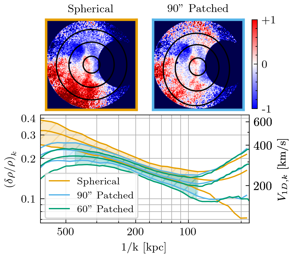
Figure 12: Effects of an asymmetric surface brightness model on measurements of $\left(\delta\rho/\rho\right)_{k}$ in the Bullet cluster. Top: Residual images within $R_{\rm 2500c}$ of the cluster using a spherical (left) and asymmetric (right; patched at a scale of $\sim$ 400 kpc = 90") $\beta$-model for the unperturbed model. Prominent substructures have been removed as in Figure 3. Bottom: The orange power spectrum corresponds to the left residual image, while the blue power spectrum corresponds to the right. The green spectrum is patched on a smaller scale to ensure that measured wavenumbers are not strongly affected by the choice of patching scale. Notations are equivalent to Figure 3.

Appendix B Supplementary figures/tables

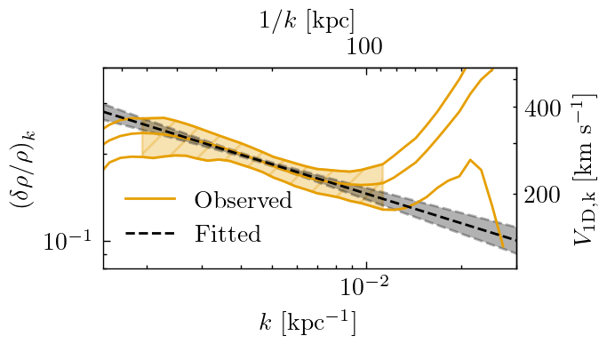
Figure 13: One example of a measured power spectrum (orange, solid lines) taken from the Bullet cluster compared to the MCMC-fitted power spectrum (black, dashed lines). $1\sigma$ uncertainties are shown in shaded regions. Notations are equivalent to Figure 3.

Here we present a version of Figure 4 with substructures included in the measurement of density fluctuations (Figure 14). We do not calculate $V_{\text{1D,k}}$ with substructures included as the $\left(\delta\rho/\rho\right)_{k}$—$V_{\text{1D,k}}$ relationship is calibrated in the bulk ICM. In this measurement, the difference in average amplitudes of density fluctuations between the relaxed and unrelaxed subsamples is much more prominent.

Additionally, for instructional purposes we display an example of an MCMC-fitted power spectrum for the Bullet cluster (Figure 13). Measured $\left(\delta\rho/\rho\right)_{k}$ is shown in orange, with best-fit $\left(\delta\rho/\rho\right)_{k}$ in black. This best-fit power spectrum is used to calculate upper limits on clumping factor, scale-independent velocity, and non-thermal pressure fraction listed in table LABEL:tab:clumpings and plotted in Figures 5 and 6.

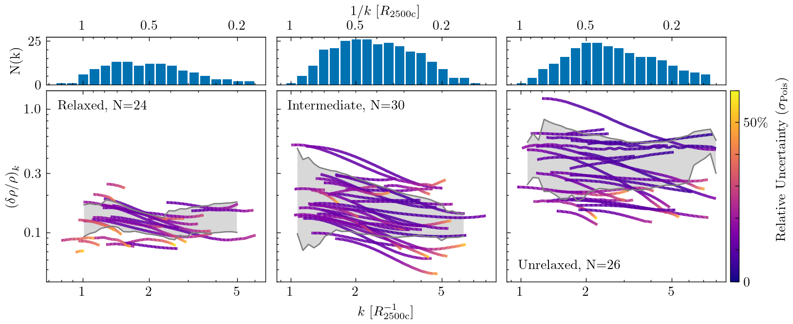
Figure 14: Equivalent to the top and middle rows of Figure 4, but with substructures included in the calculation of $\left(\delta\rho/\rho\right)_{k}$.

Table 2: Name, redshift, Chandra ObsIDs used in this work, and cleaned exposure time (in ks) for each cluster in our sample.

Cluster	Redshift	ObsIDs	Exposure
			[ks]
CygnusA	0.056	1707, 5830, 5831, 6225, 6226, 6228, 6229, 6250, 6252, 17133, 17134, 17135, 17136, 17137, 17138, 17139, 17140, 17141, 17142, 17143, 17144, 17145, 17146, 17505, 17506, 17507, 17508, 17509, 17510, 17511, 17512, 17513, 17514, 17515, 17516, 17517, 17518, 17519, 17520, 17521, 17522, 17523, 17524, 17525, 17526, 17527, 17528, 17529, 17530, 17650, 17710, 18441, 18641, 18682, 18683, 18688, 18846, 18861, 18871, 18886, 19888, 19956, 19989, 19996, 20043, 20044, 20048, 20059, 20063, 20077, 20079	2156
A1795	0.063	17225, 17226, 17228, 17230, 17231, 17232, 17610, 17611, 17612, 17615, 17618, 17622, 17624, 17625, 17628, 17629, 19871, 19873, 19874, 19875, 19939, 19972, 20646, 20647, 20648, 20650, 21833, 21834, 21835, 21838, 22832, 22834, 22835, 22836, 24603, 24605, 24606, 24607, 24608, 25049, 25672, 25676	1527
A2744	0.308	2212, 7712, 7915, 8477, 8557, 25278, 25279, 25907, 25908, 25909, 25910, 25911, 25912, 25913, 25914, 25915, 25918, 25919, 25920, 25922, 25923, 25924, 25925, 25928, 25929, 25930, 25931, 25932, 25934, 25936, 25937, 25938, 25939, 25941, 25942, 25944, 25945, 25948, 25951, 25953, 25954, 25956, 25957, 25958, 25963, 25967, 25968, 25969, 25970, 25971	1098
A2052	0.035	5807, 10477, 10478, 10479, 10480, 10879, 10914, 10915, 10916, 10917	615
A2597	0.085	6934, 7329, 19596, 19597, 19598, 20626, 20627, 20628, 20629, 20805, 20806, 20811, 20817	582
Phoenix	0.597	13401, 16135, 16545, 19581, 19582, 19583, 20630, 20631, 20634, 20635, 20636, 20797	550
Bullet	0.296	3184, 4984, 4985, 4986, 5355, 5356, 5357, 5358, 5361	524
A520	0.201	4215, 9424, 9425, 9426, 9430	512
MACS0947	0.354	7902, 22636, 22637, 22638, 22931, 22932, 22933, 22934, 22935, 23332, 24631, 24632, 24852, 24865	446
A2219	0.225	13988, 14355, 14356, 14431, 14451, 20588, 20589, 20785, 20951, 20952, 21966, 21967, 21968	444
A1367	0.022	17199, 17200, 17201, 17589, 17590, 17591, 17592, 18704, 18705, 18755	429
A3667	0.056	5751, 5752, 5753, 6292, 6295, 6296	428
A2319	0.056	3231, 15187, 23846, 24401, 24403, 24406, 24410, 24412, 24413, 24414, 24415, 24416, 24417, 27708, 27734, 27801, 27808, 27809	426
ZW0008	0.104	15318, 17204, 17205, 18242, 18243, 18244, 19901, 19902, 19905, 19916	412
A2142	0.089	5005, 7692, 15186, 16564, 16565, 17168, 17169, 17492	395
A1240	0.160	4961, 22646, 22647, 22720, 22965, 23060, 23061, 23145, 23154, 23155, 23165, 23176, 23180, 23187	351
MACS1149	0.544	3589, 16238, 16239, 16306, 16582, 17595, 17596	341
MACS0416	0.397	10446, 16236, 16237, 16304, 16523, 17313	324
A773	0.217	5006, 21540, 21541, 21542, 21543, 22043, 22044, 22045, 22051, 22052	276
A780	0.054	4969, 4970, 19570, 19571, 19997, 20007, 20968, 20969, 20970, 20971	256
A2034	0.113	2204, 7695, 12885, 12886, 13192, 13193	255
A98N	0.104	11876, 11877, 12185, 21534, 21535, 21856, 21857, 21880, 21893, 21894, 21895	248
A1664	0.128	1648, 7901, 17172, 17173, 17557, 17568	245
A1650	0.084	4178, 5822, 5823, 6356, 6357, 6358, 7242, 7691, 10424, 10425, 10426, 10427	241
A133	0.057	2203, 3183, 3710, 9897, 13518	241
MACS0717	0.546	1655, 4200, 16235, 16305	239
3C186	1.063	3098, 9407, 9408, 9774, 9775	224
ZW2341	0.283	5786, 17170, 17490, 18702, 18703	223
MACS1347	0.447	3592, 13516, 13999, 14407	208
A644	0.070	2211, 10420, 10421, 10422, 23853, 24311, 24312, 24313, 24314, 24315, 24918	207
A3847	0.153	11506, 15091, 15092, 15643	206
AS0295	0.300	12260, 16127, 16282, 16524, 16525, 16526	204
A1758N	0.279	2213, 7710, 13997, 15538, 15540	202
A85	0.055	15173, 15174, 16263, 16264	202
A3411	0.162	15316, 17193, 17496, 17497, 17583, 17584, 17585	201
MACS1206	0.440	3277, 20544, 20929, 21078, 21079, 21081	199
A401	0.074	10416, 10417, 10418, 10419, 14024, 22635, 22882	195
PKS0745	0.103	2427, 6103, 7694, 12881, 19572, 19573, 19574, 19575	190
A1835	0.253	6880, 6881, 7370	190
SPT2043	0.723	13478, 18240	187
A1689	0.183	1663, 5004, 6930, 7289, 7701	186
A2256	0.058	2419, 16129, 16514, 16515, 16516	184
A586	0.171	11723, 18278, 18279, 19961, 19962, 20003, 20004	174
ZW0104	0.119	15152, 21557, 22879, 23065, 23210	162
RXC1504	0.215	4935, 5793, 17197, 17669, 17670	161
MACS1621	0.461	3254, 3594, 6109, 6172, 7720, 9379, 10785	160
MACS0025	0.586	3251, 5010, 10413, 10786, 10797	157
3C438	0.290	3967, 12879, 13218	156
A478	0.059	1669, 6102, 6928, 6929, 7217, 7218, 7222, 7231, 7232, 7233, 7234, 7235	151
A4067	0.099	20530, 22123, 22124, 22125	149
MACS1226	0.436	3590, 12878	147
A1413	0.143	1661, 5002, 5003, 7696, 12194, 12195, 12196, 13128	146
A3112	0.075	2216, 2516, 6972, 7323, 7324, 13135	144
A665	0.182	3586, 7700, 12286, 13201, 15145, 15146, 15147, 15148	143
A1351	0.322	15136, 23845, 24296, 24297, 24298, 25101	140
A1914	0.171	3593, 18252, 20023, 20024, 20025, 20026	139
A2495	0.077	12876, 23849, 24277, 24278, 24279, 24650, 24659	137
A2626	0.055	3192, 16136	134
A2443	0.107	12257, 15169, 20625, 21437	133
MACS1423	0.545	1657, 4195	133
ZW0949	0.214	3195, 7706, 12903	126
AS1063	0.347	4966, 18611, 18818	124
A2199	0.030	10748, 10803, 10804, 10805	119
MACS2243	0.447	3260, 19749, 20129	119
MACS1931	0.352	3282, 9382	112
RXC1532	0.345	1649, 1665, 14009	108
A2204	0.151	6104, 7940, 12895, 12896, 12897, 12898	107
4C+37.11	0.055	12704, 16120	104
RXC0528	0.263	4994, 15177, 15658	104
ZW1454	0.258	4192, 7709	99
A2029	0.078	4977, 6101, 10434, 10435, 10436, 10437	98
A1300	0.307	3276, 15300, 19775, 20988, 20989, 20990	93
A2390	0.231	4193	84
RXC0439	0.230	1449, 1506, 3583, 3905, 3906	79
A2537	0.297	4962, 9372	74
MACS2140	0.313	4974, 5250	63
ZW1518	0.045	900	57
A2063	0.072	4187, 5795, 6262, 6263	50
A2151	0.037	17038, 18171, 19592, 20086, 20087	38
MACS2228	0.412	3285	20

Table 3: Cluster properties: Dynamic state (Section 2.1), chosen center coordinates, median ICM temperature in the region of interest, cluster mass ($M_{2500c}$) and radius ($R_{\rm 2500c}$), cool-core radius, total power of radio halo (if present, Section 4.2.1), and estimated Kolmogorov microscale (Section 4.2.2). Temperatures marked with $\dagger$ are measured in this work. Temperatures marked with $\ast$ are taken from projected temperature profiles.

Cluster	State	(RA,Dec)	T	$M_{\mathrm{2500c}}$	$R_{\mathrm{2500c}}$	$R_{\mathrm{cool}}$	$P_{\mathrm{1.4\ GHz}}$	$\eta_{\mathrm{K}}$	References
		[deg]	[keV]	[$10^{14}M_{\odot}$]	[kpc]	[kpc]	[$10^{24}$ W/Hz]	[kpc]
CygnusA	I	(299.8682, 40.7339)	8.1†	1.36	461	86	–	–	Comis et al.,2011 Hudson et al.,2010
A1795	I	(207.2195, 26.5906)	6.8†	3.80	597	189	–	$28^{+21}_{-11}$	Comis et al.,2011 Geng et al.,2022
A2744	U	(3.5787, -30.3906)	10.0∗	2.56	647	–	$17.4\pm 0.9$	–	Cavagnolo et al.,2008 Cavagnolo et al.,2009 Million & Allen,2009 Pearce et al.,2017
A2052	I	(229.1851, 7.0216)	3.2†	0.42	307	123	–	–	Cavagnolo et al.,2009 Comis et al.,2011
A2597	R	(351.3325, -12.1248)	4.2†	0.99	388	86	–	–	Mantz et al.,2016b Morris & Fabian,2005
Phoenix	R	(356.1825, -42.7201)	14.0	5.75	592	300	–	–	Kitayama et al.,2020 Mantz et al.,2014 McDonald et al.,2019b
Bullet	U	(104.6211, -55.9417)	10.0∗	7.41	688	–	$34.4\pm 1.1$	$13^{+36}_{-5}$	Cavagnolo et al.,2008 Cavagnolo et al.,2009 Million & Allen,2009 Sikhosana et al.,2022
A520	U	(73.5437, 2.9252)	9.0	1.76	496	–	$2.45\pm 0.18$	–	Cassano et al.,2013 Cavagnolo et al.,2009 Hicks et al.,2006 Zhu et al.,2016
MACS0947	R	(146.8039, 76.3869)	9.0	4.04	480	200	–	–	Cavagnolo et al.,2011 Comis et al.,2011 Ubertosi et al.,2023
A2219	I	(250.0850, 46.7082)	13.0	4.54	463	45	$5.63\pm 0.80$	$37^{+7}_{-14}$	Canning et al.,2017 Cassano et al.,2013 Cavagnolo et al.,2008 Cavagnolo et al.,2009
A1367	U	(176.1951, 19.7155)	3.3∗	0.65	311	–	$<0.16$	–	Farnsworth et al.,2013 Hudson et al.,2010 Phipps et al.,2019 Sanderson et al.,2006
A3667	U	(303.1458, -56.8430)	7.0∗	1.02	408	–	–	$19^{+3}_{-1}$	Akamatsu et al.,2012 Comis et al.,2011 Rossetti & Molendi,2010
A2319	I	(290.2997, 43.9470)	9.5†	2.34	538	120	–	$35^{+18}_{-14}$	Cavagnolo et al.,2009 Ettori et al.,2019
ZW0008	U	(2.9544, 52.5428)	6.5∗	0.69	353	–	–	$11^{+5}_{-4}$	Di Gennaro et al.,2019 Golovich et al.,2017
A2142	I	(239.5856, 27.2293)	8.7†	2.25	528	115	–	$24^{+22}_{-10}$	Cavagnolo et al.,2009 Comis et al.,2011
A1240	U	(170.9012, 43.1125)	4.5†∗	0.90	374	–	–	–	Cavagnolo et al.,2009 Cho et al.,2022
MACS1149	U	(177.3962, 22.4030)	10.0∗	1.50	397	–	$3.1\pm 0.9$	–	Bonafede et al.,2012 Bruno et al.,2021 Cavagnolo et al.,2009 Comis et al.,2011
MACS0416	I	(64.0389, -24.0676)	10.5	2.83	508	–	$1.06\pm 0.09$	$22^{+3}_{-2}$	Diego et al.,2015 Ogrean et al.,2015 Shitanishi et al.,2018
A773	U	(139.4716, 51.7279)	7.7	3.12	615	–	$0.90\pm 0.10$	–	Botteon et al.,2022 Cavagnolo et al.,2008 Cavagnolo et al.,2009 Zhu et al.,2016
A780	R	(139.5243, -12.0959)	3.8∗	0.80	376	150	–	–	Cavagnolo et al.,2009 Mantz et al.,2016b Sato et al.,2012
A2034	U	(227.5490, 33.5094)	8.0∗	1.94	498	–	$0.72\pm 0.09$	$25^{+26}_{-4}$	Botteon et al.,2022 Cavagnolo et al.,2009 Comis et al.,2011 Kempner et al.,2003
A98N	I	(11.6034, 20.6216)	3.0	0.38	270	100	–	–	Alvarez et al.,2022
A1664	I	(195.9266, -24.2458)	4.5	1.91	506	100	–	–	Calzadilla et al.,2019 Comis et al.,2011 Kirkpatrick et al.,2009
A1650	I	(194.6728, -1.7615)	6.2†	0.93	397	86	–	–	Cavagnolo et al.,2009 Comis et al.,2011
A133	R	(15.6743, -21.8798)	4.7†	0.71	365	92	–	–	Cavagnolo et al.,2009 Comis et al.,2011
MACS0717	U	(109.3811, 37.7576)	18.0	3.24	507	–	$22\pm 3$	$21^{+8}_{-8}$	Cavagnolo et al.,2009 Comis et al.,2011 Rajpurohit et al.,2021 Shitanishi et al.,2018
3C186	R	(116.0730, 37.8874)	7.5	1.79	320	120	–	–	Mantz et al.,2014 Mantz et al.,2016a Siemiginowska et al.,2010
ZW2341	U	(355.9203, 0.3077)	6.0∗	1.66	444	–	$0.717\pm 0.108$	–	Akamatsu & Kawahara,2013 Parekh et al.,2021 Planck Collaboration et al.,2015 Zhang et al.,2021
MACS1347	I	(206.8772, -11.7525)	16.0	10.70	783	172	–	–	Cavagnolo et al.,2009 Comis et al.,2011 Shitanishi et al.,2018
A644	I	(124.3526, -7.5076)	8.3	2.09	517	132	–	–	Cavagnolo et al.,2009 Zhu et al.,2016
A3847	R	(333.6061, -17.0264)	3.5∗	1.03	325	173	–	–	Sereno & Ettori,2017 Vagshette et al.,2017
AS0295	U	(41.3720, -53.0372)	8.5†	2.48	504	–	–	–	Pascut & Hughes,2019
A1758N	U	(203.1831, 50.5434)	9.8∗	2.56	513	–	$3.93\pm 0.53$	–	Botteon et al.,2018b Botteon et al.,2022 Cavagnolo et al.,2009 Landry et al.,2013
A85	I	(10.4604, -9.3034)	6.0†	1.29	443	107	–	–	Cavagnolo et al.,2009 Comis et al.,2011
A3411	U	(130.4922, -17.4981)	7.0	2.31	520	–	$0.27\pm 0.1$	–	Andrade-Santos et al.,2019 Cuciti et al.,2021 Zhang et al.,2020
MACS1206	I	(181.5518, -8.8023)	14.0	2.84	511	162	–	–	Cavagnolo et al.,2009 Comis et al.,2011 Shitanishi et al.,2018
A401	I	(44.7393, 13.5803)	8.1†	2.90	596	107	$0.2\pm 0.02$	$24^{+19}_{-6}$	Cavagnolo et al.,2009 Comis et al.,2011 Murgia et al.,2010
PKS0745	I	(116.8805, -19.2944)	9.0†	2.98	579	200	–	–	Cavagnolo et al.,2009 Comis et al.,2011
A1835	I	(210.2580, 2.8788)	9.2†	3.50	591	168	–	–	Cavagnolo et al.,2009 Comis et al.,2011
SPT2043	R	(310.8233, -50.5923)	6.5	1.50	360	100	–	–	McDonald et al.,2019a Sanders et al.,2018
A1689	I	(197.8731, -1.3416)	9.1†	6.22	710	198	$0.95\pm.28$	–	Cavagnolo et al.,2009 Cuciti et al.,2021 Martino et al.,2014
A2256	U	(255.9645, 78.6486)	7.5∗	1.90	509	–	$0.24\pm 0.07$	$15^{+12}_{-3}$	Comis et al.,2011 Ge et al.,2020 Hudson et al.,2010 Rajpurohit et al.,2023
A586	R	(113.0844, 31.6322)	6.8∗	1.70	309	151	–	–	Cavagnolo et al.,2009 Comis et al.,2011 Landry et al.,2013
ZW0104	U	(16.9504, 54.1360)	7.5∗	2.39	531	–	–	–	Randall et al.,2016
RXC1504	R	(226.0313, -2.8044)	10.8†	3.83	607	165	–	–	Cavagnolo et al.,2009 Comis et al.,2011
MACS1621	R	(245.3521, 38.1691)	8.5	3.06	507	160	–	–	Cavagnolo et al.,2009 Mantz et al.,2014 Mantz et al.,2016a
MACS0025	U	(6.3733, -12.3777)	9.5	2.16	431	–	–	–	Pascut & Ponman,2015 Sayers et al.,2019 Shitanishi et al.,2018
3C438	U	(328.9702, 37.9999)	8.5∗	2.35	497	–	–	–	Botteon et al.,2018a Emery et al.,2017
A478	R	(63.3567, 10.4669)	8.1†	2.80	553	171	–	–	Cavagnolo et al.,2009 Comis et al.,2011
A4067	U	(359.7048, -60.6198)	3.5∗	0.32	345	–	–	–	Cavagnolo et al.,2009 Chon & Boehringer,2015
MACS1226	I	(186.7130, 21.8316)	5.5†	1.14	370	–	–	–	De Propris et al.,2013 Ehlert,2013
A1413	R	(178.8246, 23.4057)	7.5†	1.60	465	142	–	–	Cavagnolo et al.,2009 Comis et al.,2011
A3112	R	(49.4923, -44.2368)	5.3†	0.91	392	95	–	–	Cavagnolo et al.,2009 Comis et al.,2011
A665	U	(127.7293, 65.8564)	7.5∗	1.31	433	–	$3.08\pm 0.33$	–	Botteon et al.,2022 Cavagnolo et al.,2009 Comis et al.,2011 Dasadia et al.,2016
A1351	U	(175.6025, 58.5272)	9.9†	2.25	484	–	$8.06\pm 1.01$	–	Botteon et al.,2022 Cuciti et al.,2021
A1914	U	(216.5016, 37.8257)	8.8†	5.80	683	–	$1.55\pm 0.11$	$35^{+34}_{-7}$	Cavagnolo et al.,2009 Comis et al.,2011 Mandal et al.,2019
A2495	R	(342.5828, 10.9043)	4.4†	0.90	294	70	–	–
A2626	I	(354.1266, 21.1468)	3.4†	0.43	308	66	–	–	Cavagnolo et al.,2009 Comis et al.,2011
A2443	U	(336.5180, 17.3780)	8.5∗	1.22	426	–	–	–	Clarke et al.,2013 Golovich et al.,2019 Planck Collaboration et al.,2015
MACS1423	R	(215.9495, 24.0783)	9.0	4.80	568	160	–	–	Cavagnolo et al.,2009 Comis et al.,2011 Shitanishi et al.,2018
ZW0949	R	(148.2050, 51.8847)	5.5	1.29	426	85	$<0.48$	–	Bruno et al.,2023 Cavagnolo et al.,2009 Comis et al.,2011 Mantz et al.,2016a
AS1063	I	(342.1882, -44.5285)	18.0	5.50	662	197	$2.63\pm 0.18$	–	Cavagnolo et al.,2009 Comis et al.,2011 Shitanishi et al.,2018 Xie et al.,2020
A2199	I	(247.1591, 39.5505)	4.4†	0.27	266	60	–	–	Comis et al.,2011 Kawano et al.,2003
MACS2243	U	(340.8405, -9.5947)	7.0∗	5.52	622	–	$3.2\pm 0.6$	–	Cantwell et al.,2016 Cavagnolo et al.,2009 Ehlert,2013 Parekh et al.,2017
MACS1931	I	(292.9567, -26.5761)	10.0	5.20	645	172	–	–	Cavagnolo et al.,2009 Comis et al.,2011 Shitanishi et al.,2018
RXC1532	R	(233.2242, 30.3494)	6.5	2.90	499	160	$<0.66$	–	Cassano et al.,2013 Cavagnolo et al.,2009 Comis et al.,2011 Shitanishi et al.,2018
A2204	I	(248.1958, 5.5752)	5.9†	9.20	830	131	–	–	Cavagnolo et al.,2009 Comis et al.,2011
4C+37.11	R	(61.4548, 38.0589)	5.5∗	0.82	380	97	–	$44^{+15}_{-7}$	Andrade-Santos et al.,2016
RXC0528	I	(82.2197, -39.4733)	9.1	2.50	520	96	–	–	Cavagnolo et al.,2009 Comis et al.,2011 Zhu et al.,2016
ZW1454	I	(224.3119, 22.3410)	5.0∗	1.80	460	180	–	–	Cavagnolo et al.,2009 Landry et al.,2013 Planck Collaboration et al.,2013
A2029	I	(227.7337, 5.7448)	9.2†	1.52	455	180	–	$47^{+25}_{-14}$	Cavagnolo et al.,2009 Comis et al.,2011
A1300	U	(172.9833, -19.9253)	10.5∗	3.28	552	–	$6.055\pm 0.56$	–	Cuciti et al.,2021 Kale et al.,2015 Parekh et al.,2017
A2390	I	(328.4036, 17.6951)	12.4†	8.43	701	122	–	$87^{+112}_{-59}$	Cavagnolo et al.,2009 Hicks et al.,2006
RXC0439	R	(69.7521, 7.2679)	6.5	1.84	468	100	$<0.43$	–	Cavagnolo et al.,2009 Cuciti et al.,2021 Kale et al.,2013 Mantz et al.,2016a
A2537	R	(347.0919, -2.1910)	8.8	1.37	414	104	$<0.48$	–	Cavagnolo et al.,2009 Kale et al.,2015 Zhu et al.,2016
MACS2140	R	(325.0633, -23.6611)	10.0	4.20	576	136	–	–	Cavagnolo et al.,2009 Comis et al.,2011 Shitanishi et al.,2018
ZW1518	R	(230.4660, 7.7060)	4.0†	0.67	357	122	–	–	Cavagnolo et al.,2009 Comis et al.,2011
A2063	R	(230.7704, 8.6072)	4.0†	0.90	395	96	–	–	Cavagnolo et al.,2009 Comis et al.,2011
A2151	I	(241.1490, 17.7217)	2.2†	0.19	237	29	–	–	Comis et al.,2011 Tiwari & Singh,2021
MACS2228	I	(337.1386, 20.6207)	10.5	2.15	469	146	$2.01\pm 0.22$	–	Botteon et al.,2022 Comis et al.,2011 Jia et al.,2008

References

- Akamatsu & Kawahara (2013) Akamatsu H., Kawahara H., 2013, PASJ, 65, 16
- Akamatsu et al. (2012) Akamatsu H., de Plaa J., Kaastra J., Ishisaki Y., Ohashi T., Kawaharada M., Nakazawa K., 2012, PASJ, 64, 49
- Allen et al. (2008) Allen S. W., Rapetti D. A., Schmidt R. W., Ebeling H., Morris R. G., Fabian A. C., 2008, MNRAS, 383, 879
- Alvarez et al. (2022) Alvarez G. E., Randall S. W., Su Y., Sarkar A., Walker S., Lee N. P., Sarazin C. L., Blanton E., 2022, ApJ, 938, 51
- Anders & Grevesse (1989) Anders E., Grevesse N., 1989, Geochimica Cosmochimica Acta, 53, 197
- Andrade-Santos et al. (2016) Andrade-Santos F., Bogdan A., Romani R. W., Forman W. R., Jones C., Murray S. S., Taylor G. B., Zavala R. T., 2016, ApJ, 826, 91
- Andrade-Santos et al. (2019) Andrade-Santos F., et al., 2019, ApJ, 887, 31
- Angelinelli et al. (2021) Angelinelli M., Ettori S., Vazza F., Jones T. W., 2021, A&A, 653, A171
- Arevalo et al. (2012) Arevalo P., Churazov E., Zhuravleva I., Hernandez-Monteagudo C., Revnivtsev M., 2012, MNRAS, 426, 1793
- Arnaud (1996) Arnaud K. A., 1996, ADAS&S, 101, 17
- Arnaud et al. (2010) Arnaud M., Pratt G. W., Piffaretti R., Böhringer H., Croston J. H., Pointecouteau E., 2010, A&A, 517, A92
- Arzamasskiy et al. (2023) Arzamasskiy L., Kunz M. W., Squire J., Quataert E., Schekochihin A. A., 2023, Phys Rev X, 13, 021014
- Barret et al. (2020) Barret D., Decourchelle A., Fabian A., Guainazzi M., Nandra K., Smith R., Herder J.-W. d., 2020, Astron. Nachr, 341, 224
- Battaglia et al. (2012) Battaglia N., Bond J. R., Pfrommer C., Sievers J. L., 2012, ApJ, 758, 74
- Bonafede et al. (2012) Bonafede A., et al., 2012, MNRAS, 426, 40
- Bonafede et al. (2018) Bonafede A., et al., 2018, MNRAS, 478, 2927
- Botteon et al. (2018a) Botteon A., Gastaldello F., Brunetti G., 2018a, MNRAS, 476, 5591
- Botteon et al. (2018b) Botteon A., et al., 2018b, MNRAS, 478, 885
- Botteon et al. (2022) Botteon A., et al., 2022, A&A, 660, A78
- Brunetti (2016) Brunetti G., 2016, PPCF, 58, 014011
- Brunetti & Lazarian (2007) Brunetti G., Lazarian A., 2007, MNRAS, 378, 245
- Brunetti & Lazarian (2011) Brunetti G., Lazarian A., 2011, MNRAS, 412, 817
- Brunetti et al. (2017) Brunetti G., Zimmer S., Zandanel F., 2017, MNRAS, 472, 1506
- Bruno et al. (2021) Bruno L., et al., 2021, A&A, 650, A44
- Bruno et al. (2023) Bruno L., et al., 2023, A&A, 672, A41
- Calzadilla et al. (2019) Calzadilla M. S., et al., 2019, ApJ, 875, 65
- Canning et al. (2017) Canning R. E. A., et al., 2017, MNRAS, 464, 2896
- Cantwell et al. (2016) Cantwell T. M., Scaife A. M. M., Oozeer N., Wen Z. L., Han J. L., 2016, MNRAS, 458, 1803
- Carilli & Taylor (2002) Carilli C. L., Taylor G. B., 2002, ARA&A, 40, 319
- Cassano et al. (2010) Cassano R., Ettori S., Giacintucci S., Brunetti G., Markevitch M., Venturi T., Gitti M., 2010, ApJ, 721, L82
- Cassano et al. (2013) Cassano R., et al., 2013, ApJ, 777, 141
- Cassano et al. (2023) Cassano R., et al., 2023, A&A, 672, A43
- Cavagnolo et al. (2008) Cavagnolo K. W., Donahue M., Voit G. M., Sun M., 2008, ApJ, 682, 821
- Cavagnolo et al. (2009) Cavagnolo K. W., Donahue M., Voit G. M., Sun M., 2009, ApJS, 182, 12
- Cavagnolo et al. (2011) Cavagnolo K. W., McNamara B. R., Wise M. W., Nulsen P. E. J., Brüggen M., Gitti M., Rafferty D. A., 2011, ApJ, 732, 71
- Cavaliere & Fusco-Femiano (1978) Cavaliere A., Fusco-Femiano R., 1978, A&A, 70, 677
- Cerini et al. (2022) Cerini G., Cappelluti N., Natarajan P., 2022, ApJ, 945
- Cho et al. (2022) Cho H., James Jee M., Smith R., Finner K., Lee W., 2022, ApJ, 925, 68
- Chon & Boehringer (2015) Chon G., Boehringer H., 2015, A&A, 574, A132
- Churazov et al. (2003) Churazov E., Forman W., Jones C., Böhringer H., 2003, ApJ, 590, 225
- Churazov et al. (2012) Churazov E., et al., 2012, MNRAS, 421, 1123
- Clarke et al. (2013) Clarke T. E., Randall S. W., Sarazin C. L., Blanton E. L., Giacintucci S., 2013, ApJ, 772, 84
- Clerc & Finoguenov (2023) Clerc N., Finoguenov A., 2023, X-Ray Cluster Cosmology, doi:10.1007/978-981-16-4544-0_135-1. , https://ui.adsabs.harvard.edu/abs/2023hxga.book..123C
- Comis et al. (2011) Comis B., De Petris M., Conte A., Lamagna L., De Gregori S., 2011, MNRAS, 418, 1089
- Cuciti et al. (2021) Cuciti V., et al., 2021, A&A, 647, A50
- Cui et al. (2017) Cui W., Power C., Borgani S., Knebe A., Lewis G. F., Murante G., Poole G. B., 2017, MNRAS, 464, 2502
- Dasadia et al. (2016) Dasadia S., et al., 2016, ApJ, 820, L20
- De Propris et al. (2013) De Propris R., Phillipps S., Bremer M., 2013, MNRAS, 434, 3469
- Di Gennaro et al. (2019) Di Gennaro G., et al., 2019, ApJ, 873, 64
- Diego et al. (2015) Diego J. M., Broadhurst T., Molnar S. M., Lam D., Lim J., 2015, MNRAS, 447, 3130
- Dupourqué et al. (2023) Dupourqué S., Clerc N., Pointecouteau E., Eckert D., Ettori S., Vazza F., 2023, A&A, 673, A91
- Eckert et al. (2015) Eckert D., Roncarelli M., Ettori S., Molendi S., Vazza F., Gastaldello F., Rossetti M., 2015, MNRAS, 447, 2198
- Eckert et al. (2017) Eckert D., Gaspari M., Vazza F., Gastaldello F., Tramacere A., Zimmer S., Ettori S., Paltani S., 2017, ApJ, 843, L29
- Ehlert (2013) Ehlert S. R., 2013, PhD thesis, https://ui.adsabs.harvard.edu/abs/2013PhDT.......108E
- Emery et al. (2017) Emery D. L., Bogdan A., Kraft R. P., Andrade-Santos F., Forman W. R., Hardcastle M. J., Jones C., 2017, ApJ, 834, 159
- Ettori et al. (2019) Ettori S., et al., 2019, A&A, 621, A39
- Fabian (1994) Fabian A. C., 1994, ARA&A, 32, 277
- Farnsworth et al. (2013) Farnsworth D., Rudnick L., Brown S., Brunetti G., 2013, ApJ, 779, 189
- Foreman-Mackey et al. (2013) Foreman-Mackey D., Hogg D. W., Lang D., Goodman J., 2013, PASP, 125, 306
- Forman et al. (2007) Forman W., et al., 2007, ApJ, 665, 1057
- Foster et al. (2012) Foster A. R., Ji L., Smith R. K., Brickhouse N. S., 2012, The Astrophysical Journal, 756, 128
- Gaspari et al. (2014) Gaspari M., Churazov E., Nagai D., Lau E. T., Zhuravleva I., 2014, A&A, 569, A67
- Gatuzz et al. (2023) Gatuzz E., et al., 2023, MNRAS, 522, 2325
- Gauding et al. (2014) Gauding M., Wick A., Pitsch H., Peters N., 2014, Journal of Turbulence, 15, 857
- Ge et al. (2020) Ge C., et al., 2020, MNRAS, 497, 4704
- Geng et al. (2022) Geng C., et al., 2022, MNRAS, 511, 3994
- Girardi et al. (1997) Girardi M., Fadda D., Escalera E., Giuricin G., Mardirossian F., Mezzetti M., 1997, ApJ, 490, 56
- Golovich et al. (2017) Golovich N., van Weeren R. J., Dawson W. A., Jee M. J., Wittman D., 2017, ApJ, 838, 110
- Golovich et al. (2019) Golovich N., et al., 2019, ApJ, 882, 69
- Gonzalez et al. (2021) Gonzalez E. J., Ragone-Figueroa C., Donzelli C. J., Makler M., García Lambas D., Granato G. L., 2021, MNRAS, 508, 1280
- Govoni et al. (2009) Govoni F., Murgia M., Markevitch M., Feretti L., Giovannini G., Taylor G. B., Carretti E., 2009, A&A, 499, 371
- Heinrich et al. (2021) Heinrich A., Chen Y.-H., Heinz S., Zhuravleva I., Churazov E., 2021, MNRAS, 505, 4646
- Hicks et al. (2006) Hicks A. K., Ellingson E., Hoekstra H., Yee H., 2006, ApJ, 652, 232
- Hitomi Collaboration et al. (2017) Hitomi Collaboration et al., 2017, PASJ, 70
- Hitomi Collaboration et al. (2018) Hitomi Collaboration et al., 2018, PASJ, 70
- Hlavacek-Larrondo et al. (2022) Hlavacek-Larrondo J., Li Y., Churazov E., 2022, AGN Feedback in Groups and Clusters of Galaxies, doi:10.1007/978-981-16-4544-0_122-1. , https://ui.adsabs.harvard.edu/abs/2022hxga.book....5H
- Hogg & Foreman-Mackey (2018) Hogg D. W., Foreman-Mackey D., 2018, ApJS, 236, 11
- Hu et al. (2021) Hu D., et al., 2021, ApJ, 913, 8
- Hudson et al. (2010) Hudson D. S., Mittal R., Reiprich T. H., Nulsen P. E. J., Andernach H., Sarazin C. L., 2010, A&A, 513, A37
- Ichinohe et al. (2017) Ichinohe Y., Simionescu A., Werner N., Takahashi T., 2017, MNRAS, 467, 3662
- Ishihara et al. (2016) Ishihara T., Morishita K., Yokokawa M., Uno A., Kaneda Y., 2016, Phys Rev Fluids, 1, 082403
- Jia et al. (2008) Jia S. M., Boehringer H., Pointecouteau E., Chen Y., Zhang Y. Y., 2008, A&A, 489, 1
- Johnson et al. (2012) Johnson R. E., Zuhone J., Jones C., Forman W. R., Markevitch M., 2012, ApJ, 751, 95
- Kale et al. (2013) Kale R., Venturi T., Giacintucci S., Dallacasa D., Cassano R., Brunetti G., Macario G., Athreya R., 2013, A&A, 557, A99
- Kale et al. (2015) Kale R., et al., 2015, A&A, 579, A92
- Kawano et al. (2003) Kawano N., Ohto A., Fukazawa Y., 2003, PASJ, 55, 585
- Kay & Pratt (2022) Kay S. T., Pratt G. W., 2022, Thermodynamic Profiles of Galaxy Clusters and Groups, doi:10.1007/978-981-16-4544-0_119-1. , https://ui.adsabs.harvard.edu/abs/2022hxga.book..100K
- Kelly (2007) Kelly B. C., 2007, ApJ, 665, 1489
- Kempner et al. (2003) Kempner J. C., Sarazin C. L., Markevitch M., 2003, ApJ, 593, 291
- Kirkpatrick et al. (2009) Kirkpatrick C. C., et al., 2009, ApJ, 697, 867
- Kitayama et al. (2020) Kitayama T., et al., 2020, PASJ, 72, 33
- Kraft et al. (2017) Kraft R. P., et al., 2017, ApJ, 848, 27
- Kraft et al. (2022) Kraft R., Markevitch M., Kilbourne C., team t. L., 2022, Line Emission Mapper (LEM): Probing physics of cosmic ecosystems, doi:10.48550/arXiv.2211.09827, http://arxiv.org/abs/2211.09827
- Kunz et al. (2011) Kunz M. W., Schekochihin A. A., Cowley S. C., Binney J. J., Sanders J. S., 2011, MNRAS, 410, 2446
- Kunz et al. (2022) Kunz M. W., Jones T. W., Zhuravleva I., 2022, Plasma Physics of the Intracluster Medium, doi:10.1007/978-981-16-4544-0_125-1. , https://ui.adsabs.harvard.edu/abs/2022hxga.book...56K
- Landry et al. (2013) Landry D., Bonamente M., Giles P., Maughan B., Joy M., 2013, MNRAS, 433, 2790
- Lau et al. (2009) Lau E. T., Kravtsov A. V., Nagai D., 2009, ApJ, 705, 1129
- Lau et al. (2012) Lau E. T., Nagai D., Kravtsov A. V., Vikhlinin A., Zentner A. R., 2012, ApJ, 755, 116
- Mandal et al. (2019) Mandal S., et al., 2019, A&A, 622, A22
- Mantz et al. (2014) Mantz A. B., Allen S. W., Morris R. G., Rapetti D. A., Applegate D. E., Kelly P. L., von der Linden A., Schmidt R. W., 2014, MNRAS, 440, 2077
- Mantz et al. (2015a) Mantz A. B., Allen S. W., Morris R. G., Schmidt R. W., von der Linden A., Urban O., 2015a, MNRAS, 449, 199
- Mantz et al. (2015b) Mantz A. B., Allen S. W., Morris R. G., Schmidt R. W., von der Linden A., Urban O., 2015b, MNRAS, 449, 199
- Mantz et al. (2016a) Mantz A. B., Allen S. W., Morris R. G., 2016a, MNRAS, 462, 681
- Mantz et al. (2016b) Mantz A. B., et al., 2016b, MNRAS, 463, 3582
- Markevitch & Vikhlinin (2007) Markevitch M., Vikhlinin A., 2007, Physics Reports, 443, 1
- Markevitch et al. (2002) Markevitch M., Gonzalez A. H., David L., Vikhlinin A., Murray S., Forman W., Jones C., Tucker W., 2002, ApJ, 567, L27
- Martino et al. (2014) Martino R., Mazzotta P., Bourdin H., Smith G. P., Bartalucci I., Marrone D. P., Finoguenov A., Okabe N., 2014, MNRAS, 443, 2342
- McDonald et al. (2019a) McDonald M., et al., 2019a, ApJ, 870, 85
- McDonald et al. (2019b) McDonald M., et al., 2019b, ApJ, 885, 63
- Million & Allen (2009) Million E. T., Allen S. W., 2009, MNRAS, 399, 1307
- Mohapatra et al. (2020) Mohapatra R., Federrath C., Sharma P., 2020, MNRAS, 493, 5838
- Mohapatra et al. (2021) Mohapatra R., Federrath C., Sharma P., 2021, MNRAS, 500, 5072
- Mohr et al. (1999) Mohr J., Mathiesen B., Evrard G., 1999, ApJ, 517, 627
- Morris & Fabian (2005) Morris R. G., Fabian A. C., 2005, MNRAS, 358, 585
- Murgia et al. (2010) Murgia M., Govoni F., Feretti L., Giovannini G., 2010, A&A, 509, A86
- Nagai & Lau (2011) Nagai D., Lau E. T., 2011, ApJ, 731, L10
- Nagai et al. (2007a) Nagai D., Vikhlinin A., Kravtsov A. V., 2007a, ApJ, 655, 98
- Nagai et al. (2007b) Nagai D., Kravtsov A. V., Vikhlinin A., 2007b, ApJ, 668, 1
- Nelson et al. (2014a) Nelson K., Lau E. T., Nagai D., Rudd D. H., Yu L., 2014a, ApJ, 782, 107
- Nelson et al. (2014b) Nelson K., Lau E. T., Nagai D., 2014b, ApJ, 792, 25
- Nishiwaki & Asano (2022) Nishiwaki K., Asano K., 2022, ApJ, 934, 182
- Nulsen et al. (2013) Nulsen P. E. J., et al., 2013, ApJ, 775, 117
- Ogorzalek et al. (2017) Ogorzalek A., et al., 2017, MNRAS, 472, 1659
- Ogrean et al. (2015) Ogrean G., et al., 2015, ApJ, 812, 153
- Owers et al. (2013) Owers M. S., et al., 2013, ApJ, 780, 163
- Parekh et al. (2017) Parekh V., Dwarakanath K. S., Kale R., Intema H., 2017, MNRAS, 464, 2752
- Parekh et al. (2021) Parekh V., et al., 2021, MNRAS, 509, 3086
- Pascut & Hughes (2019) Pascut A., Hughes J. P., 2019, ApJ, 874, 71
- Pascut & Ponman (2015) Pascut A., Ponman T. J., 2015, MNRAS, 447, 3723
- Pearce et al. (2017) Pearce C. J. J., et al., 2017, ApJ, 845, 81
- Petrosian & Bykov (2008) Petrosian V., Bykov A. M., 2008, Space Sci Rev, 134, 207
- Phipps et al. (2019) Phipps F., Bogdan A., Lovisari L., Kovács O. E., Volonteri M., Dubois Y., 2019, ApJ, 875, 141
- Planck Collaboration et al. (2013) Planck Collaboration et al., 2013, A&A, 550, A129
- Planck Collaboration et al. (2015) Planck Collaboration et al., 2015, A&A, 581, A14
- Pratt et al. (2019) Pratt G. W., Arnaud M., Biviano A., Eckert D., Ettori S., Nagai D., Okabe N., Reiprich T. H., 2019, Space Sci Rev, 215, 25
- Rajpurohit et al. (2021) Rajpurohit K., et al., 2021, A&A, 646, A135
- Rajpurohit et al. (2023) Rajpurohit K., et al., 2023, A&A, 669, A1
- Randall et al. (2016) Randall S. W., et al., 2016, ApJ, 823, 94
- Rebusco et al. (2005) Rebusco P., Churazov E., Böhringer H., Forman W., 2005, MNRAS, 359, 1041
- Romero et al. (2023) Romero C. E., et al., 2023, ApJ, 951, 41
- Rossetti & Molendi (2010) Rossetti M., Molendi S., 2010, A&A, 510, A83
- Sanders & Fabian (2013) Sanders J. S., Fabian A. C., 2013, MNRAS, 429, 2727
- Sanders et al. (2018) Sanders J. S., Fabian A. C., Russell H. R., Walker S. A., 2018, MNRAS, 474, 1065
- Sanders et al. (2020) Sanders J. S., et al., 2020, A&A, 633, A42
- Sanderson et al. (2006) Sanderson A. J. R., Ponman T. J., O’Sullivan E., 2006, MNRAS, 372, 1496
- Sarazin (1988) Sarazin C. L., 1988, X-ray emission from clusters of galaxies. https://ui.adsabs.harvard.edu/abs/1988xrec.book.....S
- Sato et al. (2012) Sato T., et al., 2012, PASJ, 64, 95
- Sayers et al. (2019) Sayers J., et al., 2019, ApJ, 880, 45
- Schekochihin & Cowley (2006) Schekochihin A. A., Cowley S. C., 2006, Physics of Plasmas, 13, 056501
- Schmidt et al. (2001) Schmidt R. W., Allen S. W., Fabian A. C., 2001, MNRAS, 327, 1057
- Schuecker et al. (2004) Schuecker P., Finoguenov A., Miniati F., Boehringer H., Briel U. G., 2004, A&A, 426, 387
- Sereno & Ettori (2017) Sereno M., Ettori S., 2017, MNRAS, 468, 3322
- Shi et al. (2015) Shi X., Komatsu E., Nelson K., Nagai D., 2015, MNRAS, 448, 1020
- Shitanishi et al. (2018) Shitanishi J. A., et al., 2018, MNRAS, 481, 749
- Siemiginowska et al. (2010) Siemiginowska A., Burke D. J., Aldcroft T. L., Worrall D. M., Allen S., Bechtold J., Clarke T., Cheung C. C., 2010, ApJ, 722, 102
- Sikhosana et al. (2022) Sikhosana S. P., Knowles K., Hilton M., Moodley K., Murgia M., 2022, MNRAS, 518, 4595
- Simonte et al. (2022) Simonte M., Vazza F., Brighenti F., Brüggen M., Jones T. W., Angelinelli M., 2022, A&A, 658, A149
- Smith et al. (2001) Smith R. K., Brickhouse N. S., Liedahl D. A., Raymond J. C., 2001, The Astrophysical Journal, 556, L91
- Spitzer (1962) Spitzer L., 1962, Physics of Fully Ionized Gases. https://ui.adsabs.harvard.edu/abs/1962pfig.book.....S
- Su et al. (2017) Su Y., et al., 2017, ApJ, 834, 74
- Tiwari & Singh (2021) Tiwari J., Singh K. P., 2021, MNRAS, 500, 5524
- Ubertosi et al. (2023) Ubertosi F., et al., 2023, ApJ, 944, 216
- Umetsu et al. (2018) Umetsu K., et al., 2018, ApJ, 860, 104
- Vacca et al. (2011) Vacca V., Govoni F., Murgia M., Giovannini G., Feretti L., Tugnoli M., Verheijen M. A., Taylor G. B., 2011, A&A, 535, A82
- Vagshette et al. (2017) Vagshette N. D., Naik S., Patil M. K., Sonkamble S. S., 2017, MNRAS, 466, 2054
- Vazza et al. (2017) Vazza F., Jones T. W., Brüggen M., Brunetti G., Gheller C., Porter D., Ryu D., 2017, MNRAS, 464, 210
- Vazza et al. (2018) Vazza F., Angelinelli M., Jones T. W., Eckert D., Brüggen M., Brunetti G., Gheller C., 2018, MNRAS, 481, L120
- Vikhlinin et al. (2005) Vikhlinin A., Markevitch M., Murray S. S., Jones C., Forman W., Van Speybroeck L., 2005, ApJ, 628, 655
- Vikhlinin et al. (2009) Vikhlinin A., et al., 2009, ApJ, 692, 1033
- Walker et al. (2015) Walker S. A., Sanders J. S., Fabian A. C., 2015, MNRAS, 453, 3699
- Walker et al. (2018) Walker S. A., Sanders J. S., Fabian A. C., 2018, MNRAS, 481, 1718
- Walker et al. (2019) Walker S., et al., 2019, Space Sci Rev, 215, 7
- Watanabe & Gotoh (2007) Watanabe T., Gotoh T., 2007, Phys. Fluids, 19, 121701
- Werner et al. (2016) Werner N., et al., 2016, MNRAS, 455, 846
- XRISM Science Team (2020) XRISM Science Team 2020, Science with the X-ray Imaging and Spectroscopy Mission (XRISM), http://arxiv.org/abs/2003.04962
- Xie et al. (2020) Xie C., et al., 2020, A&A, 636, A3
- Yeung et al. (2002) Yeung P. K., Xu S., Sreenivasan K. R., 2002, Phys. Fluids, 14, 4178
- Yeung et al. (2014) Yeung P. K., Zhai X. M., Sreenivasan K. R., 2014, APS Division of Fluid Dynamics Meeting Abstracts, p. H27.001
- Yuan et al. (2022) Yuan Z. S., Han J. L., Wen Z. L., 2022, MNRAS, 513, 3013
- Zhang et al. (2020) Zhang X., Simionescu A., Akamatsu H., Kaastra J. S., de Plaa J., van Weeren R. J., 2020, A&A, 642, A89
- Zhang et al. (2021) Zhang X., et al., 2021, A&A, 656, A59
- Zhang et al. (2022) Zhang X., et al., 2022, A&A
- Zhu et al. (2016) Zhu Z., et al., 2016, ApJ, 816, 54
- Zhuravleva et al. (2013) Zhuravleva I., Churazov E., Kravtsov A., Lau E. T., Nagai D., Sunyaev R., 2013, MNRAS, 428, 3274
- Zhuravleva et al. (2014a) Zhuravleva I., et al., 2014a, Nature, 515, 85
- Zhuravleva et al. (2014b) Zhuravleva I., et al., 2014b, ApJ, 788, L13
- Zhuravleva et al. (2015) Zhuravleva I., et al., 2015, MNRAS, 450, 4184
- Zhuravleva et al. (2018) Zhuravleva I., Allen S. W., Mantz A. B., Werner N., 2018, ApJ, 865, 53
- Zhuravleva et al. (2019) Zhuravleva I., Churazov E., Schekochihin A. A., Allen S. W., Vikhlinin A., Werner N., 2019, Nat Astron, 3, 832
- Zhuravleva et al. (2023) Zhuravleva I., Chen M. C., Churazov E., Schekochihin A. A., Zhang C., Nagai D., 2023, MNRAS
- ZuHone & Su (2022) ZuHone J., Su Y., 2022, The Merger Dynamics of the X-Ray-Emitting Plasma in Clusters of Galaxies, doi:10.1007/978-981-16-4544-0_124-1. , https://ui.adsabs.harvard.edu/abs/2022hxga.book...93Z
- Zuhone & Roediger (2016) Zuhone J. A., Roediger E., 2016, Journal of Plasma Physics, 82, 535820301
- de Gasperin et al. (2022) de Gasperin F., et al., 2022, A&A, 659, A146
- de Vries et al. (2023) de Vries M., et al., 2023, MNRAS, 518, 2954
- van Weeren et al. (2019) van Weeren R. J., de Gasperin F., Akamatsu H., Brüggen M., Feretti L., Kang H., Stroe A., Zandanel F., 2019, Space Sci Rev, 215, 16