Collective dynamical Fermi suppression of optically-induced inelastic scattering

Abstract

We observe strong dynamical suppression of optically-induced loss in a weakly interacting Fermi gas as the $s$-wave scattering length is increased. The single, cigar-shaped cloud behaves as a large spin lattice in energy space with a tunable Heisenberg Hamiltonian. The loss suppression occurs as the lattice transitions into a magnetized state, where the fermionic nature of the atoms inhibits interactions. The data are quantitatively explained by incorporating spin-dependent loss into a quasi-classical collective spin vector model, the success of which enables the application of optical control of effective long-range interactions to this system.

Optically-induced loss plays an important role in the optical control of two-body scattering interactions in quantum gases [1, 2, 3, 4]. These techniques enable designer quantum simulators that exploit the high spatial and temporal resolution that is possible with optical fields. For weakly interacting Fermi gases prepared in coherent spin superposition states, optical control offers new prospects for creating designer Hamiltonians in a quasi-continuous system. In this system, individual atoms remain in their energy states $\phi_{E}(x)$ over experimental time scales, creating a long-lived synthetic lattice [5] with pseudo-spins pinned at sites labeled by $E$ in energy space to simulate a collective Heisenberg Hamiltonian [6, 7, 8, 9, 10, 11, 12, 13, 14, 15]. Effective long-range site-to-site, i.e., $E$ to $E^{\prime}$, interactions arise from the overlap in real space of the probability densities $|\phi_{E}(x)|^{2}$ and $|\phi_{E^{\prime}}(x)|^{2}$ with the $s$-wave scattering length $a_{S}(x,t)$, which is tunable in space and time by two-field optical control near a magnetic Feshbach resonance [4]. This method employs electromagnetically-induced transparency to optimize the tradeoff between tunability and spontaneous optical scattering [3], but finite spontaneous scattering remains, causing site and spin-dependent atom loss that must be understood to apply optical control.

The Pauli principle plays an essential role in the evolution of the loss, as a pair of fermionic atoms cannot undergo inelastic $s$-wave scattering when the spin state of a colliding atom pair is symmetric. This becomes especially relevant when the synthetic spin lattice evolves into a magnetized state, which occurs at a sufficiently large scattering length [12, 16]. Fermi gases have recently provided new demonstrations of the Pauli principle in degenerate samples, including the suppression of light scattering [17, 18, 19] and the suppression of stimulated emission [20], which arise from Pauli blocking, where optical momentum transfer to single atoms is inhibited by occupied final momentum states. In contrast, Fermi suppression of light scattering in a weakly interacting Fermi gas emerges from effective long range spin-spin interactions and is both dynamical and collective.

In this paper, we examine the collective suppression of optically-induced inelastic scattering in a weakly interacting ⁶Li Fermi gas. The cloud is coherently excited by a radiofrequency (RF) $\pi/2$ pulse to prepare a superposition of the two lowest hyperfine states denoted by $|1\rangle\equiv|\!\!\uparrow_{z}\rangle$ and $|2\rangle\equiv|\!\!\downarrow_{z}\rangle$. A bias magnetic field $B$ tunes the trapped cloud near the zero crossing of the $s$-wave scattering length via a magnetic Feshbach resonance. Loss is induced by an optical field that excites a molecular state $|g\rangle$, which is responsible for the Feshbach resonance, to an electronically-excited molecular state, denoted $|e\rangle$ [2, 3, 4]. For a sufficiently large $s$-wave scattering length, the cloud undergoes a transition from high to low loss. We develop a model for the spin-dependent loss, which shows that dynamical loss suppression arises from the onset of a magnetized state. This work paves the way for the application of optical control to create customized Hamiltonians in weakly interacting Fermi gases and generally provides a model for understanding two-body loss for large spin systems in collective time-dependent superposition states.

Our measurements employ a ⁶Li Fermi gas, containing $N=6\times 10^{4}$ spin-polarized atoms. The gas is confined in a cigar-shaped optical trap and cooled to temperature $T=0.18\,T_{F}$, where the Fermi temperature $T_{F}\simeq 0.75\,\mu$K. The small ratio between the transverse ($\rho$) Thomas-Fermi radius, $\simeq 12\,\mu$m, and the axial ($x$) Thomas-Fermi radius, $\simeq 330\,\mu$m, enables a quasi-1D approximation in the model.

For the small $s$-wave scattering lengths $a_{S}(B)$ employed in the experiments, forward scattering dominates and the rate of energy-changing collisions is negligible during each experimental cycle. In the absence of loss, atoms remain fixed in their respective energy states, allowing the system to be described as a 1D lattice in energy space, where atoms in a group with nearly the same axial energy $E$ evolve identically and are described by a collective spin vector $\mathbf{S}(E,t)$ [8, 21]. Without loss, the evolution of $\mathbf{S}(E)$ is described by the spin Hamiltonian $H(E)=\boldsymbol{\omega}(E)\cdot\mathbf{S}(E)$, where

$$\boldsymbol{\omega}(E)=\Omega^{\prime}E\,\hat{\mathbf{e}}_{z}+\sum_{E^{\prime}\neq E}g(E,E^{\prime})\,\mathbf{S}(E^{\prime}).$$ (1)

The evolution is determined by effective long range spin-spin interactions with a coupling $g(E,E^{\prime})\propto a_{S}$ and by a site-dependent Zeeman precession rate $\Omega^{\prime}E=-\delta\omega_{x}E/(\hbar\omega_{x})$. $\Omega^{\prime}$ arises from curvature in the bias magnetic field along the axial $x$ direction, which produces a spin-dependent harmonic potential that is comparable to the optical confining potential. In our experiments, the average coupling $\bar{g}\simeq 1.6$ Hz $\times\,2\pi$ for $a_{S}=5.0\,a_{0}$ and the rms spread in $\Omega^{\prime}\,E$, denoted $\Omega^{\prime}\sigma_{E}$, is $\simeq 1.4$ Hz$\,\times\,2\pi$. As the interaction strength $\zeta\equiv\bar{g}/(\Omega^{\prime}\sigma_{E}\sqrt{2})$ is increased, the system exhibits a phase transition into a magnetized state [21].

Defining $\mathbf{S}(E,t)=S(E,t)\,\hat{\mathbf{S}}(E,t)$, where $\hat{\mathbf{S}}(E,t)$ is a unit vector and $S(E,t)=N_{E}(t)/2$ with $N_{E}(t)$ the number of atoms with axial energy $E$,

$$\dot{\mathbf{S}}(E)=S(E)\,\dot{\hat{\mathbf{S}}}(E)+\dot{S}(E)\,\hat{\mathbf{S}}(E).$$ (2)

Neglecting loss, where $\dot{S}(E)=0$, the rotation of $\mathbf{S}(E)$, given by first term in Eq. 2, is determined by the Heisenberg equations,

$$\dot{\hat{\mathbf{S}}}(E,t)=\boldsymbol{\omega}(E,t)\times\hat{\mathbf{S}}(E,t).$$ (3)

We solve Eq. S1 for the unit vectors $\hat{\mathbf{S}}(E,t)$ in a quasi-classical approximation, treating $\mathbf{S}(E,t)$ and $\mathbf{S}(E^{\prime},t)$ as classical vectors, In our experiments, an initial $\pi/2$ RF pulse coherently prepares $\mathbf{S}(E,0)$ to be polarized in the transverse plane, orthogonal to the bias magnetic field.

Eqs. 1 and S1 show that each collective spin vector $\mathbf{S}(E,t)$ rotates about an effective magnetic field vector, comprising an applied magnetic field component along $\hat{\mathbf{e}}_{z}$ and a net mean field component arising from forward $s$-wave scattering interactions with all other $\mathbf{S}(E^{\prime},t)$. For small $a_{S}$, where the energy-dependent precession rate about the magnetic field dominates, the spin vectors fan out in the transverse plane, reducing the effect of the mean-field. This is reflected in a low magnitude of the total spin vector $S(t)=|\sum_{E}\mathbf{S}(E,t)|$, as shown in Fig. 1. For sufficiently large $a_{S}$, the mean-field becomes significant, suppressing the energy-dependent spreading of the collective spin vectors, which effectively orbit the mean-field. However, the effect of the mean field degrades as the spin vectors align, as there is no longer any rotation about the mean field axis. This again allows the spread in the Zeeman precession rates to separate the spin vectors, which allows the rotation about the mean field to dominate again, leading to an oscillation of the magnitude of the total spin vector, as shown in Fig. 1. We see that for larger $a_{S}$, where the mean-field dominates and most spin vectors align, the amplitude of the oscillation is smallest, corresponding to a transition to a magnetized state [12, 16]. Note that in our experiments a $z$-polarized sample is coherently excited by a $\pi/2$ RF pulse, which results in $S_{z}(t)\equiv\sum_{E}S_{z}(E,t)=0$ and therefore $S(t)=\sqrt{S_{\perp}(t)^{2}+S_{z}(t)^{2}}=S_{\perp}(t)$.

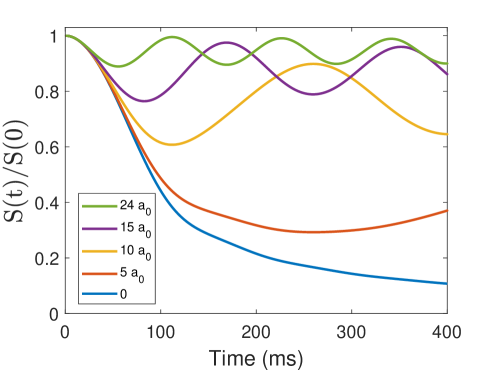
Figure 1: Predicted magnitude the total spin vector versus time for loss-free evolution with different $s$-wave scattering lengths. $N=6.0\times 10^{4}$ atoms and the zero-temperature Thomas-Fermi widths for the axial and radial directions are $330.0\,\mu$m and $12.0\,\mu$m, respectively. Since $S_{z}(t)=0$ when the spins are prepared orthogonal to the applied magnetic field, $S(t)=S_{\perp}(t)$, the length of the transverse (XY plane) projection of the total spin vector.

Inelastic scattering is induced in the energy lattice by applying an optical field tuned near resonance with the $|g\rangle\rightarrow|e\rangle$ transition [3], as mentioned above. Without the optical field, the state of an incoming pair of free atoms, nominally in the electronic triplet channel [3, 21], is hyperfine coupled to $|g\rangle$ in the electronic singlet channel. The optical field induces a finite probability to be in state $|e\rangle$, which decays by spontaneous emission to low lying molecular states. In a non-interacting or weakly-interacting gas, as used in the experiments, this process causes loss of both atoms, without heating or pumping into higher- or lower-energy trap modes. With the energy-lattice picture retained, the evolution of the collective spin vectors is no longer simply a rotation, as $\dot{S}(E,t)=\dot{N}_{E}(t)/2\neq 0$ in Eq. 2. To incorporate loss into the model, we must compute $N_{E}(t)$.

Loss due to two-body inelastic collisions between two species $A$ and $B$ with 3D densities $n_{A}(\mathbf{r},t)$ and $n_{B}(\mathbf{r},t)$ is generally modeled as

$$\dot{n}_{A}(\mathbf{r},t)=\dot{n}_{B}(\mathbf{r},t)=-K_{2}^{AB}n_{A}(\mathbf{r},t)n_{B}(\mathbf{r},t),$$ (4)

which follows from the definition of the $AB$ inelastic cross section $\sigma_{inel}^{AB}$, i.e., $K_{2}^{AB}\equiv\langle v_{rel}\sigma_{inel}^{AB}\rangle$, where the brackets denote the average over the relative speed $v_{rel}$. In the energy-space lattice, each energy corresponds to a definite spin. In our quasi-classical picture, atoms of axial energy $E$, in the spin state $|\hat{\mathbf{S}}(E)\rangle$, collide with atoms of energy $E^{\prime}$ in the spin state $|\hat{\mathbf{S}}(E^{\prime})\rangle$ for all $E^{\prime}\neq E$. To find $N_{E}(t)$, we generalize Eq. S10 to model the loss of the spin-energy correlated 3D densities $n_{E}(\mathbf{r},t)$, i.e., the density of atoms with axial energy $E$:

$$\dot{n}_{E}(\mathbf{r},t)=-\sum_{E^{\prime}}K(E,E^{\prime}\!,t)\,n_{E}(\mathbf{r},t)\,n_{E^{\prime}}(\mathbf{r},t),$$ (5)

where $K(E,E^{\prime}\!,t)$ is the effective loss rate coefficient. Spin-dependent Fermi suppression is manifested in our expression for $K(E,E^{\prime},t)$, which weights the two-body loss coefficient $K_{2}^{a}$ associated with the anti-symmetric total spin state $|\Psi_{a}(1,2)\rangle$ by the probability that the incoming two-atom spin state $|\hat{\mathbf{S}}(E)\rangle_{1}|\hat{\mathbf{S}}(E^{\prime})\rangle_{2}$ is in the state $|\Psi_{a}(1,2)\rangle$ [21],

$$K(E,E^{\prime}\!,t)=\frac{K_{2}^{a}}{4}[1-\hat{\mathbf{S}}(E,t)\cdot\hat{\mathbf{S}}(E^{\prime},t)].$$ (6)

In the quasi-classical approximation, dynamical suppression of loss appears in the time dependence of the unit vectors, $\hat{\mathbf{S}}(E,t)$. $K(E,E^{\prime},t)$ has a maximum of $K_{2}^{a}/2$ when the colliding spin vectors are anti-parallel and vanishes when the spin vectors are parallel, which is most likely for a magnetized state.

To determine $N_{E}(t)$ from Eq. 5, we employ a quasi-1D approximation, where the 3D density factors [21]: $n_{E}(\mathbf{r},t)=n_{E}(\rho,x,t)\simeq N_{E}(t)\mathcal{R}(\rho,t)|\phi_{E}(x)|^{2}$. Here $x$ is the axial coordinate and $\rho$ is is the radial coordinate. We take $\mathcal{R}(\rho,t)$ to be the normalized transverse probability density, $\int d\rho\,2\pi\rho\,\mathcal{R}(\rho,t)=1$ for all $t$ and $\int d^{3}\mathbf{r}\,n_{E}(\mathbf{r},t)=N_{E}(t)$. Integrals of Eq. 5 over $\rho$ and $x$ result in coupled equations for $\dot{\mathcal{R}}(\rho,t)$ and $\dot{N}_{E}(t)$  [21]. Density-dependent loss causes $N_{E}(t)$ to decrease in time and $\mathcal{R}(\rho,t)$ to change shape, affecting the average transverse probability density $\bar{n}_{\perp}(t)=\int d\rho\,2\pi\rho\,[\mathcal{R}(\rho,t)]^{2}$. The evolution equations for $S(E,t)=N_{E}(t)/2$, $\hat{\mathbf{S}}(E,t)$, and $\mathcal{R}(\rho,t)$ determine the evolution of the total atom number $N(t)=\sum_{E}N_{E}(t)$.

We note that including the time-dependence of $\bar{n}_{\perp}(t)$ is essential, since $g(E,E^{\prime},t)\propto\bar{n}_{\perp}(t)$ [8, 21], altering the net rotation rate of the collective spin vectors, Eq. 1. Further, the time dependence of $\bar{n}_{\perp}(t)$ significantly alters the loss rate, as demonstrated by comparing data to predictions for $\bar{n}_{\perp}=\bar{n}_{\perp}(t)$ with those for $\bar{n}_{\perp}=\bar{n}_{\perp}(0)$ [21].

To test the loss model, we measure the time-dependent loss of the total atom number $N(t)$ for scattering lengths $a_{S}=0$ to $24$ Bohr ($a_{0}$), corresponding to interaction strengths from $\zeta=0$ to 5.39. The trapped gas is illuminated by a nominally uniform optical field resonant with the $|g\rangle\rightarrow|e\rangle$ transition and evolves for a variable amount of time before resonant absorption imaging of the atom densities for the spectrally resolved $|\!\!\uparrow_{z}\rangle$ and $|\!\!\downarrow_{z}\rangle$ states.

The gas is prepared in the weakly interacting regime as described in reference Ref. [8]. We use the calibration from Ref. [8] to tune to the desired scattering length $a(B)$, where RF spectroscopy precisely determines $B$. Immediately following a $0.5$ ms $\pi/2$ RF pulse, a loss-inducing optical field is applied and the system evolves for a time $0\leq t\leq 400$ ms. The Rabi frequency of the optical field is estimated to be [21] $\Omega_{1}=\gamma_{e}/2$, where $\gamma_{e}=2\pi\times 11.8$ MHz is the spontaneous emission rate from the excited molecular state $e$. Since the optical field is on resonance, there is no optical shift of the scattering length [4]. The trap frequencies are $\omega_{\rho}=2\pi\times 668$ Hz and $\omega_{x}=2\pi\times 25$ Hz. A fit to a zero-temperature Thomas-Fermi profile yields an axial width $\sigma_{TF}=330\,\mu$m. The radial width of 12 $\mu$m is computed from the ratio of the trap frequencies. For each measurement with a coherently prepared sample, the two-body loss rate coefficient $K_{2}$ is measured for a 50-50 mixture. These measured values of $K_{2}$ are used as inputs into the loss model.

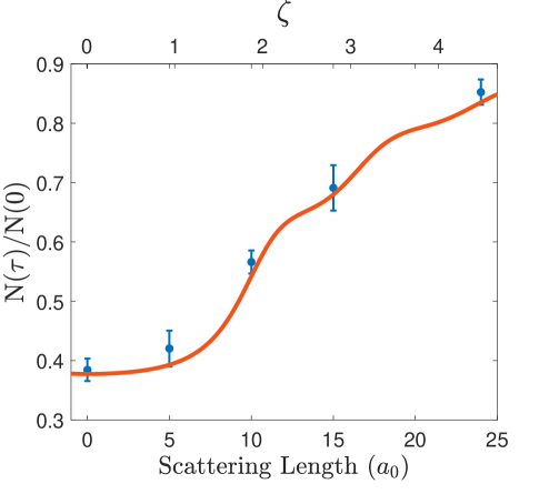
Figure 2: Measurements of the atom fraction remaining after $\tau=370$ ms of illumination as the scattering length is increased (blue points), compared to the theoretical prediction (red curve). The densities and values of $K_{2}^{a}$ vary slightly for each measurement (see [21]). For the prediction, the averaged values of $N(0)=6.1\times 10^{4}$ atoms, $\sigma_{TF}=332\,\mu$m, and $K_{2}^{a}=62\,\mu$m³/s are used. The data are also plotted versus the interaction strength $\zeta$, defined in the text.

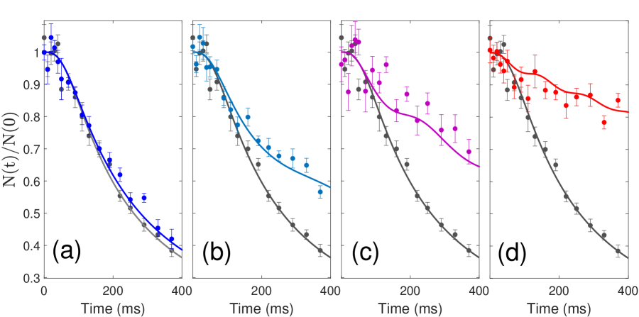
Figure 3: Suppression of optically-induced loss versus illumination time as the scattering length is increased. $N(t)/N(0)$ is the atom fraction remaining after a time $t$. As a reference, the data and model for the non-interacting gas $a_{S}=0\,a_{0}$ ($\zeta=0$) are shown in black on each plot. Each point represents the average of six shots, and the error bar is the standard deviation of the mean. (a) $a_{S}=5\,a_{0}$ ($\zeta=1.03$), (b) $a_{S}=10\,a_{0}$ ($\zeta=2.32$), (c) $a_{S}=15\,a_{0}$ ($\zeta=3.59$), (d) $a_{S}=24\,a_{0}$ ($\zeta=5.39$). Note that the interaction strength $\zeta$ does not change exactly linearly in the scattering length due to slight variations in the atom number and width. The measured values of $K_{2}$ and exact densities for each scattering length are given in [21].

The fraction of atoms remaining after $\tau=370$ ms of illumination, $N(\tau)/N(0)$, is shown in Fig. 2 for the different scattering lengths. The data demonstrate the phase transition to a magnetized state, and the Fermi suppression more than doubles the number of atoms remaining between the $a_{S}=\,$0 and 24 $a_{0}$ cases. Error bars represent the standard deviation of the mean for six shots. The prediction generated by the loss model (red curve) agrees well with the data. For the prediction, we use the averaged atom number, axial widths, and values of $K_{2}$ from the measurements.

Measurements of the fraction of atoms remaining throughout the evolution $N(t)/N(0)$ for coherently prepared samples are shown in Fig. 3, along with the corresponding predictions using no free parameters. Predictions and measurements for $a_{S}=0\,a_{0}\,(\zeta=0)$, where interactions are absent, are shown as a reference, and agree very well. With scattering lengths $a_{S}$ of 0, 5 $(\zeta=1.03)$, and 10 $a_{0}$ $(\zeta=2.32)$, for which the system never becomes strongly magnetized, the atom number is nearly stagnant for the first $\approx\,$80 ms, corresponding to the time needed for the energy-dependent Zeeman precession rates to separate the collective spin vectors. Once the spin vectors are sufficiently separated, the effective loss rate coefficient $K(E,E^{\prime},t)$ becomes non-negligible and the atom number begins to decay. At $a_{S}=5\,a_{0}$, the data are almost indistinguishable from the $a_{S}=0\,a_{0}$ case, Fig. 3a. This is consistent with Fig. 1, where, for $a_{S}=5\,a_{0}$ at our experimental densities, the system is still in the energy-dependent precession-dominated regime. The data show that a phase transition out of this regime occurs between $a_{S}=5\,a_{0}$ and $a_{S}=10\,a_{0}$, where the measurements at $a_{S}=10\,a_{0}$ exhibit the onset of loss suppression, Fig. 3b. The loss is further suppressed for the $a_{S}=15\,a_{0}\,(\zeta=3.59)$ data, Fig. 3c, and even more for the $a_{S}=24\,a_{0}\,(\zeta=5.39)$ data, Fig. 3d, reflecting the increasing collective alignment of the spins, as depicted for the lossless case of Fig. 1.

Our collective spin vector model of loss for the energy-space lattice is in good quantitative agreement with measurements. The average of the values of $K_{2}^{a}$ used to generate the curves in Fig. 3, $\,62\,\pm\,6.2\,\mu\text{m}^{3}/s$, is in good agreement with the predicted value of $69.4\,\mu{\rm m}^{3}/s$  [21]. However, we find that the values of $K_{2}^{a}$ used in the model need to be half of those extracted from measurements in a 50-50 mixture. For the 50-50 mixture, we assume that given pair of atoms collides in a product state, with a probability of $1/2$ to be in the antisymmetric spin state [21], making the extracted $K_{2}^{a}$ twice as large. This origin of this discrepancy his not yet clear. Further, we have assumed that the simple two-body loss model used for the mixture measurement may be trivially applied to the weakly interacting regime.

In summary, we have observed dynamical collective suppression of optically-induced inelastic scattering in a coherently-prepared, weakly-interacting Fermi gas. As the scattering length is increased at fixed initial density, we observe a transition from high to low loss. We understand this suppression via the Pauli principle, where the system makes a transition into a magnetized state with parallel collective spin vectors, Fig. 1, causing suppression of $s$-wave scattering. In this way, loss suppression serves as a new probe of the magnetization of the system. We have developed a loss model that quantitatively agrees with observations and incorporates the many-body evolution of the collective spin vectors. This model explains the loss accompanying the optical tailoring of Hamiltonians in weakly interacting Fermi gases.

Primary support for this research is provided by the Air Force Office of Scientific Research (FA9550-22-1-0329). Additional support is provided by the National Science Foundation (PHY-2006234 and PHY-2307107).

^∗Corresponding author: jethoma7@ncsu.edu

Appendix A Supplemental Material

In this supplemental material, we begin by reviewing the energy-space spin lattice model for the evolution of collective spin vectors in a weakly interacting Fermi gas without loss. Then we describe a generalized model, including two-body loss for the collective, energy-dependent spin vectors, which is compared to measurements in coherently prepared samples. Finally, we describe the experimental methods and the measurement of the optically-induced, two-body loss rate constant $K_{2}$ in two-state mixtures.

Appendix B Evolution of the Energy-Space Spin Lattice without Loss

In the weakly interacting regime, the $s$-wave scattering length $a_{S}$ is magnetically tuned to be sufficiently small that the collision rate is negligible over the experimental time scales. In this case, the energies of individual atoms are conserved, enabling an energy-space spin-lattice description [8, 6]. For a cigar-shaped optical trap, the lattice can be approximated as one-dimensional, where the collective spin vectors $\mathbf{S}(E,t)$ are labeled by the axial energy $E$ for motion along the cigar axis, defined as $x$. The energy-space spin-lattice is described by a Heisenberg Hamiltonian, where the corresponding Heisenberg equations of motion yield an $E$-dependent rotation for the collective spin vector $\mathbf{S}(E,t)$ at each site. In a mean-field description, the rotation arises from an effective site $E$-dependent Zeeman field and the effective magnetic field arising from the spin-spin coupling to all other sites $E^{\prime}\neq E$. We employ a quasi-classical description, where $\mathbf{S}(E,t)$ is treated as a classical vector.

The experiments employ a ⁶Li Fermi gas in a superposition of the two lowest hyperfine-Zeeman states, which are denoted $|1\rangle\equiv|\uparrow_{z}\rangle$ and $|2\rangle\equiv|\downarrow_{z}\rangle$. The curvature of the applied bias magnetic field, $\partial^{2}_{x}B_{z}$, and the difference in the magnetic moments for the two hyperfine states produce a spin-dependent axial harmonic trap frequency and a corresponding $E$-dependent rotation rate about the applied magnetic field, which we denote by $\mathbf{\Omega_{B}}(E)=\Omega^{\prime}E\,\hat{\mathbf{z}}$. The site-to-site coupling, denoted by $g(E,E^{\prime})$, arises from forward s-wave scattering.

Taking $\mathbf{S}(E,t)=S(E,t)\,\hat{\mathbf{S}}(E,t)$, where $\hat{\mathbf{S}}(E,t)$ denotes a unit vector, we find

$$\dot{\hat{\mathbf{S}}}(E,t)=\mathbf{\Omega_{B}}(E)\times\hat{\mathbf{S}}(E,t)+\sum_{E^{\prime}}\,g(E,E^{\prime})\,\mathbf{S}(E^{\prime},t)\times\hat{\mathbf{S}}(E,t).$$ (S1)

Without loss, each $\mathbf{S}(E,t)$ evolves via rotation. In this case, the magnitudes $|\mathbf{S}(E,t)|\equiv S(E,t)=S(E,t=0)$ are conserved. There is some flexibility in the definition of $S(E)$, as Eq. S1 is invariant under the scale transformation $S(E)\rightarrow c(E)\,S(E)$ and $g(E,E^{\prime})\rightarrow g(E,E^{\prime})/c(E)$. We choose $S(E,t=0)$ to be

$$S(E,t=0)=N_{E}/2.$$ (S2)

Here $N_{E}=N\,P(E)$ is the number of atoms in axial energy group $E$, with $N$ the total atom number and $P(E)$ the probability distribution. In the model, we take $P(E)$ to be a zero-temperature Thomas-Fermi distribution for near-degenerate samples; for higher temperatures, we employ a Boltzmann distribution. The collective spin vectors begin their evolution after a $\pi/2$ RF pulse coherently rotates the initially $z$-polarized sample, so that

$$\hat{\mathbf{S}}(E,t=0)=\mathbf{\hat{x}^{\prime}},$$ (S3)

where $\mathbf{\hat{x}^{\prime}}$ is defined in the Bloch frame, orthogonal to $\mathbf{\hat{z}}$.

For our choice of $S(E,t=0)$ in Eq. S2, the site-to-site couplings $g(E,E^{\prime})$ in Eq. S1 are given by

$$g(E,E^{\prime})=-\bar{n}_{\perp}\frac{8\pi\hbar}{m}\,\int dx\,|\phi_{E}(x)|^{2}|\phi_{E^{\prime}}(x)|^{2}\,a_{S}$$ (S4)

where $\phi_{E}(x)$ is the axial trap eigenstate for energy $E$. Note that optical control of interactions allows $a_{S}\rightarrow a_{S}(x,t)$, so that $g(E,E^{\prime})$ may be tailored. In Eq. S4, we have assumed that the single-particle probability density takes the form $\mathcal{R}(\rho)\,|\phi_{E}(x)|^{2}$, where $x$ is the axial coordinate, $\rho$ is the transverse radial coordinate, $\mathcal{R}(\rho)$ is the transverse probability density, and $\int d\rho\,2\pi\rho\,\mathcal{R}(\rho)=1$. The overlap integral is evaluated using a WKB approximation. For a harmonic trap,

$$\int dx\,|\phi_{E}(x)|^{2}|\phi_{E^{\prime}}(x)|^{2}=\frac{2}{\pi^{2}}\sqrt{\frac{m\bar{\omega}_{x}^{2}}{2|E-E^{\prime}|}}\,{\rm EllipticK}\left[-\frac{\text{min}(E,E^{\prime})}{|E-E^{\prime}|}\right],$$ (S5)

In Eq. S4, $\bar{n}_{\perp}$ is the average transverse probability density,

$$\bar{n}_{\perp}\equiv\int d\rho\,2\pi\rho\,\mathcal{R}^{2}(\rho).$$ (S6)

For lossless evolution, $\mathcal{R}(\rho)$ is time-independent. Assuming a zero-temperature Thomas-Fermi distribution,

$$\mathcal{R}(\rho)=\frac{3}{\pi\sigma_{\rho}^{2}}\left(1-\frac{\rho^{2}}{\sigma_{\rho}^{2}}\right)^{2}$$ (S7)

we obtain $\bar{n}_{\perp}=9/(5\pi\sigma_{\rho}^{2})$. For the Maxwell-Boltzmann distribution,

$$\mathcal{R}(\rho)=\frac{1}{\pi\sigma_{\rho}^{2}}\,e^{-\rho^{2}/\sigma_{\rho}^{2}},$$ (S8)

we find $\bar{n}_{\perp}=1/(\pi\sigma_{\rho}^{2})$.

Appendix C Modeling Two-Body Loss in the Energy-Space Spin lattice

Inelastic interactions are induced in the energy-space spin lattice by illuminating the coherently prepared clouds with an optical field. In this section, we describe our model for the loss in this system due to these interactions.

We begin by describing the interaction process: For the magnetic fields of interest, a collision between a pair of ⁶Li atoms, one in each of the two lowest hyperfine spin states, occurs nominally in the triplet electronic potential (where “triplet” refers to the two-electron spin state). For $s$-wave scattering, where the relative motion state is symmetric in the interchange of the two atoms, the two-atom hyperfine state is the antisymmetric state,

$$|\Psi_{a}(1,2)\rangle=\frac{1}{\sqrt{2}}\,\left(|\uparrow_{z}\rangle_{1}\,|\downarrow_{z}\rangle_{2}-|\downarrow_{z}\rangle_{1}|\uparrow_{z}\rangle_{2}\right)\simeq|1,-1;1,1\rangle.$$ (S9)

At high magnetic fields, as used in the experiments, $|1,-1;1,1\rangle$ is the dominant triplet state in the interior basis, i.e., the total electronic spin state is $S=1,M_{S}=-1$, the total nuclear spin state is $I=1,M_{I}=1$. This triplet state has a large hyperfine coupling to the dominant singlet electronic state $S=0$ [22], denoted $|g\rangle$, which is in the $38^{\rm th}$ vibrational state of the singlet ground molecular potential, producing a broad Feshbach resonance at 832.2 G [23]. The difference between the magnetic moments of the singlet and triplet states enables magnetic tuning of the $s$-wave scattering length near the resonance. The applied optical field drives transitions from $|g\rangle$ to the $64^{\rm th}$ electronically-excited vibrational state in the electronic singlet molecular potential, denoted $|e\rangle$ [2, 3]. Spontaneous emission from $|e\rangle$ causes the interaction to be inelastic, and we assume that the emission results in loss of both atoms without transfer of atoms between energy states, so that the energy-space spin lattice model remains appropriate.

Loss due to two-body inelastic collisions between a particle of species $A$ and a particle of species $B$ is generally modeled as

$$\dot{n}_{A}(\mathbf{r},t)=\dot{n}_{B}(\mathbf{r},t)=-K_{2}^{AB}n_{A}(\mathbf{r},t)n_{B}(\mathbf{r},t)$$ (S10)

where $n_{A}(\mathbf{r},t)$ is the 3D density of species $A$ and $n_{B}(\mathbf{r},t)$ is the 3D density of species $B$. It is assumed that only $A$ and $B$ interact, and that each inelastic collisions causes both atoms to be lost. Eq. S10 follows from the definition of the inelastic cross section of the $AB$ interaction $\sigma_{inel}^{AB}$ where $K_{2}^{AB}\equiv\langle v_{rel}\sigma_{inel}^{AB}\rangle$ (the brackets denote the average over the relative speeds $v_{rel}$). This will be our basis for constructing our loss model.

C.1 Optically-Induced Loss in the Energy Lattice

To treat loss in the energy-space spin lattice, we consider the atoms at each energy site $E$ to be a “species” in the context of Eq. S10. We associate a 3D density $n_{E}(\mathbf{r},t)$ to the group of atoms with energy $E$ and a collective spin vector $\mathbf{S}(E,t)$, and sum the inelastic collision rates for atoms of energy with $E$ with atoms of energies $E^{\prime}$ over all $E^{\prime}\neq E$ to obtain

$$\dot{n}_{E}(\mathbf{r},t)=-\sum_{E^{\prime}}K(E,E^{\prime}\!,t)\,n_{E^{\prime}}(\mathbf{r},t)\,n_{E}(\mathbf{r},t).$$ (S11)

Here the total density is $n(\mathbf{r},t)=\sum_{E}n_{E}(\mathbf{r},t)$ and $K(E,E^{\prime}\!,t)$ is the effective energy-dependent two-body loss rate coefficient.

We obtain $K(E,E^{\prime}\!,t)$ by computing the probability that the pair of atoms in energy groups $E$ and $E^{\prime}$ are in the antisymmetric spin state $|\Psi_{a}(1,2)\rangle$. We assume that the spin of each atom of energy $E$ is polarized along $\mathbf{S}(E,t)$, corresponding to the spin state $|\hat{\mathbf{S}}(E,t)\rangle$. In this case, atoms of energies $E$ and $E^{\prime}$ are in states with definite spin polarizations, so that we can assume the incoming spin state for a colliding pair of atoms with energies $E$ and $E^{\prime}$ is $|\hat{\mathbf{S}}(E,t)\rangle_{1}\,|\hat{\mathbf{S}}(E^{\prime},t)\rangle_{2}$. The probability amplitude to be in the singlet state is then found by the inner product of this state with $|\Psi_{a}(1,2)\rangle$, so that

$$K(E,E^{\prime}\!,t)=K_{2}^{a}\,|\langle\Psi_{a}(1,2)|\hat{\mathbf{S}}(E,t)\rangle_{1}\,|\hat{\mathbf{S}}(E^{\prime},t)\rangle_{2}|^{2}.$$ (S12)

where $K_{2}^{a}$ is the loss constant associated with the antisymmetric two-atom spin state, given in Eq. S9. Suppressing the time dependence, the energy-dependent spin states take the form,

$$|\hat{\mathbf{S}}(E)\rangle_{1} = e^{-i\phi_{E}/2}\cos(\theta_{E}/2)\,|\!\!\uparrow_{z}\rangle_{1}\,+\,e^{i\phi_{E}/2}\sin(\theta_{E}/2)\,|\!\!\downarrow_{z}\rangle_{1}$$

$$|\hat{\mathbf{S}}(E^{\prime})\rangle_{2} = e^{-i\phi_{E}^{\prime}/2}\cos(\theta_{E}^{\prime}/2)\,|\!\!\uparrow_{z}\rangle_{2}\,+\,e^{i\phi_{E}^{\prime}/2}\sin(\theta_{E}^{\prime}/2)\,|\!\!\downarrow_{z}\rangle_{2}.$$ (S13)

A straightforward calculation gives

$$|\langle\Psi_{a}(1,2)|\hat{\mathbf{S}}(E,t)\rangle_{1}\,|\hat{\mathbf{S}}(E^{\prime},t)\rangle_{2}|^{2}=\frac{1}{4}\,\left[1-\cos\theta_{E}\cos\theta_{E^{\prime}}-\sin\theta_{E}\sin\theta_{E^{\prime}}\cos(\phi_{E}-\phi_{E^{\prime}})\right],$$ (S14)

or, in terms of the unit vectors and restoring the time dependence,

$$K(E,E^{\prime}\!,t)\equiv\frac{K_{2}^{a}}{4}\left[1-\hat{\mathbf{S}}(E,t)\cdot\hat{\mathbf{S}}(E^{\prime},t)\right].$$ (S15)

As expected, when the collective spin vectors for energy groups $E$ and $E^{\prime}$ vectors are parallel, the corresponding unit vectors $\hat{\mathbf{S}}(E,t)$ and $\hat{\mathbf{S}}(E^{\prime},t)$ are parallel and there is no loss. In contrast, maximum loss occurs when the unit vectors are anti-parallel, $K(E,E^{\prime},t)\rightarrow K_{2}^{a}/2$ . The unit vectors $\hat{\mathbf{S}}(E,t)$ are found from Eq. S1, with $S(E,t)=N_{E}(t)/2$, where the atom number $N_{E}(t)$ is self-consistently determined from Eqs. S11 and S15, as we now show.

We begin by assuming that the spin-energy correlated 3D densities $n_{E}(\mathbf{r},t)$ can be factored as

$$n_{E}(\mathbf{r},t)=n_{E}(x,\rho,t)=N_{E}(t)\,\mathcal{R}(\rho,t)\,|\phi_{E}(x)|^{2},$$ (S16)

where $x$ is the axial coordinate and $\rho$ the transverse coordinate. As observed in the experiments and shown in Fig. S2 below, for nonzero $K_{2}^{a}$, the increase in the loss rate with increasing 3D density reshapes the spatial profile. For this reason, we assume that both the atom number $N_{E}(t)$ in each energy group and the transverse probability density $\mathcal{R}(\rho,t)$ are functions of time. Further, we assume that $\mathcal{R}(\rho,t)$ is independent of $E$, and take $\int d\rho\,2\pi\rho\,\mathcal{R}(\rho,t)=1$ for all $t$. Using Eq. S16, the spatial integral of the total density, $n(\mathbf{r},t)=\sum_{E}n_{E}(\mathbf{r},t)$ yields total atom number,

$$N(t)=\sum_{E}N_{E}(t).$$ (S17)

Using Eq. S16 in Eq. S11 and integrating over $x$, we obtain

$$\frac{d}{dt}\left[N_{E}(t)\mathcal{R}(\rho,t)\right]=-\sum_{E^{\prime}}\eta(E,E^{\prime},t)\left[N_{E^{\prime}}(t)\mathcal{R}(\rho,t)\right]\,\left[N_{E}(t)\mathcal{R}(\rho,t)\right],$$ (S18)

where

$$\eta(E,E^{\prime}\!,t)\equiv K(E,E^{\prime}\!,t)\int dx\,|\phi_{E}(x)|^{2}|\phi_{E^{\prime}}(x)|^{2}.$$ (S19)

Integrating Eq. S18 over $\rho$ and using Eq. S21, we find

$$\dot{N}_{E}(t)\int d\rho\,2\pi\rho\,\mathcal{R}(\rho,t)+N_{E}(t)\frac{d}{dt}\int d\rho\,2\pi\rho\,\mathcal{R}(\rho,t)=-\bar{n}_{\perp}(t)\,\sum_{E^{\prime}}\eta(E,E^{\prime}\!,t)\,N_{E^{\prime}}(t)\,N_{E}(t),$$ (S20)

where $\bar{n}_{\perp}(t)$ is the time-dependent average transverse probability density

$$\bar{n}_{\perp}(t)\equiv\int d\rho\,2\pi\rho\,\mathcal{R}^{2}(\rho,t).$$ (S21)

Since $\int d\rho\,2\pi\rho\,\mathcal{R}(\rho,t)=1$, Eq. S20 immediately yields

$$\dot{N}_{E}(t)=-\bar{n}_{\perp}(t)\,\sum_{E^{\prime}}\eta(E,E^{\prime}\!,t)\,N_{E^{\prime}}(t)\,N_{E}(t).$$ (S22)

Next, we sum Eq. S18 over $E$ and use Eq. S17 to obtain

$$\dot{N}(t)\,\mathcal{R}(\rho,t)+N(t)\,\dot{\mathcal{R}}(\rho,t)=-\mathcal{R}^{2}(\rho,t)\sum_{E}\sum_{E^{\prime}}\eta(E,E^{\prime}\!,t)\,N_{E^{\prime}}(t)\,N_{E}(t)=\dot{N}(t)\,\frac{\mathcal{R}^{2}(\rho,t)}{\bar{n}_{\perp}(t)}.$$ (S23)

Here, the right-hand side has been simplified by using the sum of Eq. S22 over $E$ and Eq. S17,

$$\dot{N}(t)=-\bar{n}_{\perp}(t)\,\sum_{E}\sum_{E^{\prime}}\eta(E,E^{\prime}\!,t)\,N_{E^{\prime}}(t)\,N_{E}(t).$$ (S24)

Hence, the radial probability distribution obeys

$$\dot{\mathcal{R}}(\rho,t)=\frac{\dot{N}(t)}{N(t)}\left[\frac{\mathcal{R}^{2}(\rho,t)}{\bar{n}_{\perp}(t)}-\mathcal{R}(\rho,t)\right].$$ (S25)

Using Eq. S21, one readily verifies that the integral of Eq. S25 over $\rho$ vanishes, so that the total transverse probability remains normalized to $1$ for all $t$. Further, the right hand side is $\propto\dot{N}(t)\,[\mathcal{R}(\rho,t)-\bar{n}_{\perp}(t)]$, where $\dot{N}(t)<0$ when $K_{2}^{a}\neq 0$. Hence, near the center of the cloud, where $\mathcal{R}(\rho,t)>\bar{n}_{\perp}(t)$, the probability density decreases in time, while in the wings, where $\mathcal{R}(\rho,t)<\bar{n}_{\perp}(t)$, the probability density increases in time. The net effect of the loss is to increase the effective width of $\mathcal{R}(\rho,t)$, while preserving the normalization.

C.2 Optically-Induced Loss in a Mixture

For the loss model described above, we require the loss constant $K_{2}^{a}$ associated with a pair of atoms in the antisymmetric two-atom spin state $|\Psi_{a}(1,2)\rangle$. To obtain $K_{2}^{a}$, we measure the loss in a 50-50 incoherent mixture of $|\uparrow_{z}\rangle$ and $\,|\downarrow_{z}\rangle$, for which the 50-50 ratio is maintained throughout the evolution, and extract the fraction of the loss constant associated with the state $|\Psi_{a}(1,2)\rangle$. Considering the mixture to be comprised of atoms in the $|\uparrow_{z}\rangle$ state and the $|\downarrow_{z}\rangle$ state, we define the 3D densities associated with each state $n_{\uparrow}(\mathbf{r},t)$ and $n_{\downarrow}(\mathbf{r},t)$ and apply Eq. S10 to obtain

$$\dot{n}_{\uparrow}(\mathbf{r},t)=\dot{n}_{\downarrow}(\mathbf{r},t)=-K_{2}^{\uparrow\downarrow}n_{\uparrow}(\mathbf{r},t)n_{\downarrow}(\mathbf{r},t).$$ (S26)

We assume that the incoming state is a product state $|\uparrow_{z}\rangle_{1}|\downarrow_{z}\rangle_{2}$. Then, the probability to be in the antisymmetric two-atom spin state is $|\langle\Psi_{a}(1,2)|\uparrow_{z}\rangle_{1}|\downarrow_{z}\rangle_{2}|^{2}=1/2$,

$$K_{2}^{\uparrow\downarrow}=K_{2}^{a}\times 1/2.$$ (S27)

With $n_{\uparrow}(\mathbf{r},t)+n_{\downarrow}(\mathbf{r},t)=n(\mathbf{r},t)$ the total density and $n_{\uparrow}(\mathbf{r},t)=n_{\downarrow}(\mathbf{r},t)=n(\mathbf{r},t)/2$ for a 50-50 mixture, Eq. S26 yields

$$\dot{n}(\mathbf{r},t)=-\frac{1}{4}K_{2}^{a}\,n^{2}(\mathbf{r},t).$$ (S28)

Eq. S28 may be solved analytically:

$$n(\mathbf{r},t)=\frac{n(\mathbf{r},0)}{1+\frac{1}{4}\,K^{a}_{2}n(\mathbf{r},0)\,t}.$$ (S29)

Integrating Eq. S29 over all three spatial dimensions, the total atom number $N(t)$ is predicted as a function of time, given $n(\mathbf{r},0)$:

$$N(t)=\int\!dx\int\!2\pi\rho\,d\rho\,\frac{n(\mathbf{r},0)}{1+\frac{1}{4}\,K_{2}^{a}n(\mathbf{r},0)\,t}.$$ (S30)

To measure $K_{2}^{a}$, then, we fit measurements of the atom number $N(t)$ in the 50-50 mixture to Eq. S30. This is further described in § E.2, where we show that $K_{2}^{a}$ is independent of the relative speed near the zero crossing of the broad Feshbach resonance in ⁶Li, see Eq. S39. However, as will also be discussed in § E.2, we must halve the measured $K_{2}^{a}$ before inserting it into Eq. S14 in order to reach agreement with the loss measurements in the energy lattice.

Appendix D Evolution of the Energy-Space Spin Lattice with Loss

To model the energy-space lattice with optically-induced loss, we employ Eqs. S22 and S25, together with Eq. S1. These equations determine the evolution of the density for each energy group, the transverse profile and therefore the total density and the total number in the presence of loss, which are compared with the measurements.

Including the $E$-dependent loss, the magnitudes of the collective spin vectors in Eq. S1, $S(E,t)=N_{E}(t)/2$, decrease with time. The evolution of $\mathbf{S}(E,t)$ includes both a rotation of the unit vectors and a time-dependent magnitude,

$$\dot{\mathbf{S}}(E,t)=S(E,t)\,\dot{\hat{\mathbf{S}}}(E,t)+\dot{S}(E,t)\,\hat{\mathbf{S}}(E,t).$$ (S31)

The unit vectors $\hat{\mathbf{S}}(E,t)$ evolve according to Eq. S1, while the decay of the magnitudes $S(E,t)$ is determined by Eq. S22 with $N_{E}(t)=2\,S(E,t)$ and Eqs. S19 and S15,

$$\dot{S}(E,t)=-\sum_{E^{\prime}}\kappa(E,E^{\prime}\!,t)\,\left[S(E,t)S(E^{\prime},t)-\mathbf{S}(E,t)\cdot\mathbf{S}(E^{\prime},t)\right].$$ (S32)

Here, the effective loss rate $\kappa(E,E^{\prime}\!,t)$ is given by

$$\kappa(E,E^{\prime}\!,t)\equiv\frac{K_{2}^{a}}{2}\,\bar{n}_{\perp}(t)\int dx\,|\phi_{E}(x)|^{2}|\phi_{E^{\prime}}(x)|^{2}.$$ (S33)

We discuss the measurement of $K_{2}^{a}$ for mixtures in § E.2.

We rewrite the evolution of the transverse probability density, Eq. S25, as

$$\dot{\mathcal{R}}(\rho,t)=\frac{\dot{S}(t)}{S(t)}\left[\frac{\mathcal{R}^{2}(\rho,t)}{\bar{n}_{\perp}(t)}-\mathcal{R}(\rho,t)\right].$$ (S34)

Here we have defined $S(t)\equiv\sum_{E}S(E,t)=N(t)/2$. Eq. S21 shows that the site-to-site couplings of Eq. S4 become time dependent for $K_{2}^{a}\neq 0$, $g(E,E^{\prime})\rightarrow g(E,E^{\prime},t)$, while the decay of $S(E,t)$ reduces the rotation rate of the unit vectors by reducing the magnitude of the mean field.

Including loss, the evolution of the energy-dependent collective spin vectors is determined by Eq. S31, using Eq. S1 to describe the rotation of the unit vectors and Eqs. S32, S34, and S21 to determine the decay of the magnitudes. The collective spin vectors are initialized according to Eqs. S2 and S3. The initial condition for the transverse probability density, $\mathcal{R}(\rho,0)$, is given by Eq. S7 for a Thomas-Fermi distribution and by Eq. S8 for a Maxwell-Boltzmann distribution.

Appendix E Experimental Methods

E.1 Measurement of Loss in the Energy-Space Spin Lattice

To test the loss model, we measure the time-dependent decay of the total atom number $N(t)$ in a cigar-shaped optical trap comprising a single focused CO₂ laser beam. The measurements are obtained for scattering lengths $a_{S}=0\,a_{0}$ to $24\,a_{0}$ at nominally the same density. Starting from a $\hat{\mathbf{z}}$-polarized sample, we employ a $0.5$ ms $\pi/2$ RF pulse to prepare an initially $\mathbf{\hat{x}^{\prime}}$-polarized sample as described in § B. Immediately following the RF pulse, the trapped gas is illuminated by a uniform optical field locked on-resonance with the singlet molecular $g\rightarrow e$ transition (see § C) and evolves for a variable amount of time $t$ before absorption imaging of the atom densities for the $|\uparrow_{z}\rangle$ and $|\downarrow_{z}\rangle$ states, which are spectrally resolved.

In the experiments, we begin by evaporatively cooling a 50-50 mixture of atoms in the two lowest hyperfine states $|\uparrow\rangle_{z}\equiv|1\rangle$ and $|\downarrow\rangle_{z}\equiv|2\rangle$ at the broad Feshbach resonance near 832.2 G [23]. Following forced evaporation by lowering the trap depth, the trap depth is increased so that the radial trap frequency is $\omega_{\rho}=2\pi\times 668.0$ Hz. To avoid the formation of Feshbach molecules while tuning to the weakly interacting region near 527 G, the magnetic field is swept up to 1200 G and resonant light is applied to expel one spin state, leaving a $\hat{\mathbf{z}}$-polarized spin sample. The magnetic field is then swept to produce scattering length $a_{S}(B)$ of interest near $527$ G. The calibration of Ref. [8] determines $a_{S}(B)$, where magnetic field is measured by RF spectroscopy.

After this preparation, the total number of atoms $N(0)\simeq 6.0\times 10^{4}$. A fit of the measured axial profile with a zero-temperature Thomas-Fermi distribution yields an axial width $\sigma_{TF}^{x}\simeq 331\,\mu$m, Fig. S1. The radial width $\sigma_{TF}^{\rho}$ is computed from the ratio of trap transverse and axial frequencies, $\omega_{\rho}\sigma_{TF}^{\rho}=\omega_{x}\sigma_{TF}^{x}$. As noted in § B, the curvature in the applied magnetic field results in a spin-dependent axial trapping force in the axial direction, where $\omega_{mag}=2\pi\times 16.3$ Hz. For the combined optical and magnetic trapping potentials near 527 G, the net axial trap frequency is measured to be $\omega_{x}=2\pi\times 25.0$ Hz. With $\omega_{\rho}=2\pi\times 668.0$ Hz, we find $\sigma_{TF}^{\rho}\simeq 12.0\,\mu$m.

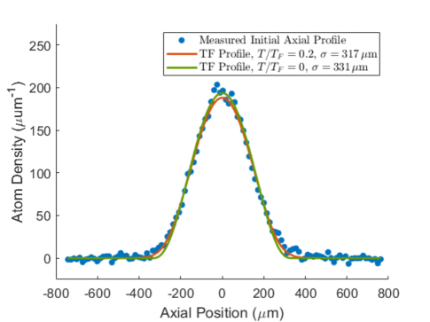
Figure S1: Thomas-Fermi fits to the sum of the initial axial profiles of the $|\uparrow_{z}\rangle$ and $|\downarrow_{z}\rangle$ states, immediately after the $\pi/2$ pulse, as used for measurement of $N(t)$ at 0 Bohr in the coherently-prepared sample. The fit of a finite-temperature 1D Thomas-Fermi profile yields the reduced temperature $T/T_{F}=0.2$. The fit is nearly identical to that of a zero-temperature 1D Thomas Fermi profile, justifying our use to a zero-temperature distribution in the model.

To determine the temperature, we fit a 1-D finite-temperature Thomas-Fermi distribution to the initial axial profile. The Fermi temperature $T_{F}$ for our harmonic trap is determined by

$$E_{F}=k_{B}T_{F}=\hbar\,(6N\omega_{\rho}^{2}\omega_{x})^{1/3}.$$ (S35)

Note that the 6 in Eq. S35 reflects the fact that all $N$ atoms initially begin in an identical spin state. For the initial atom number and trap frequencies given in the last paragraph, we find $T_{F}\simeq 0.75\,\mu$K. Using the calculated Thomas-Fermi radius $\sigma_{TF}=\sqrt{2E_{F}/(m\omega_{x}^{2})}\simeq 317.0\,\mu$m, a fit to a finite-temperature Thomas-Fermi profiles yields $T\simeq 0.20\,T_{F}$. Fig. S1 shows the averaged initial axial profile for a sample that is coherently prepared at 0 Bohr, along with the corresponding fitted finite-temperature 1D Thomas-Fermi and zero-temperature 1D Thomas-Fermi profiles. The zero-temperature and finite-temperature Thomas-Fermi profiles are nearly identical, as expected for $T\simeq 0.20\,T_{F}$, justifying the use of an effective zero-temperature profile with a fitted width in the model.

For every scattering length, $K_{2}^{a}$ is measured from the loss in a 50-50 mixture, as discussed in § E.2. Loss is induced by an optical beam propagating at an angle of $\simeq 49^{\circ}$ relative to the trap $x$-axis. The intensity half width at 1/e of the optical beam is $w=1.1$ mm, so that the projection of the full width of the optical beam at 1/e onto the cloud $x-axis$, is $2\,w\sin(49^{\circ})\simeq 1.5\,w=1.6$ mm. This can be compared to the full width of the cloud $2\,\sigma_{x}\simeq 0.66$ mm. Hence, most of the atoms are illuminated near the peak intensity, $I=P/(\pi w^{2})$. The servo-stabilized beam power is $7.6$ mW, so that $I=2.0$ mW/mm². The Rabi frequency for the singlet electronic transition from the ground $38^{\rm th}$ vibrational state $|g\rangle$ to the excited $64^{\rm th}$ vibrational state has been measured [4] to be $\Omega_{1}/2\pi=4.4$ MHz  $\sqrt{I{\rm[mW/mm}^{2}]}$. The Rabi frequency for the loss inducing beam is then $\Omega_{1}=0.53\times\gamma_{e}$, where $\gamma_{e}=2\pi\times 11.8$ MHz is the rate of spontaneous emission from the excited molecular state [3, 2]. The resonance frequency for each magnetic field value is found by finding the peak loss in the incoherent mixture as a function of frequency, which is prepared as described in § E.2. Since the optical field is locked on resonance, there is no optical shift in the scattering length.

The importance of including the time dependence of $\mathcal{R}(\rho,t)$ in the model can be seen in the difference between the predictions for $\bar{n}_{\perp}=\bar{n}_{\perp}(0)$ and $\bar{n}_{\perp}=\bar{n}_{\perp}(t)$ at $a_{S}=0\,a_{0}$, as shown in Fig. S2. If $\bar{n}_{\perp}$ is taken to be constant, the model disagrees with the data for longer times. Accounting for the decrease in $\bar{n}_{\perp}(t)$ reduces the energy-dependent loss rate $\kappa(E,E^{\prime}\!,t)$ of Eq. S33, causing the tail of the loss curve to rise to match the data.

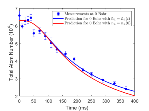
Figure S2: Predictions of loss in a coherently-prepared sample, with (blue) and without (red) the time dependence of the average transverse probability density $\bar{n}_{\perp}$. The time-dependence of $\bar{n}_{\perp}(t)$ arises from loss. Measurements for 0 Bohr in the coherently-prepared cloud are in agreement with the model when $\bar{n}_{\perp}=\bar{n}_{\perp}(t)$ (blue). When $\bar{n}_{\perp}$ is taken to be constant (red), the tail of the loss curve does not agree with the measurements. For the 0 Bohr data, the inputs into the loss model are $K_{2}^{a}=58.0\,\mu m^{3}/s$, the initial atom number $N=6.3\times 10^{4}$ and the width $\sigma_{TF}=331.0\,\mu$m.

E.2 Measurement of the Two-Body Loss Constant $K_{2}^{a}$ in a Mixture

To measure the two-body loss constant $K_{2}^{a}$, we measure the decay of the total number of atoms in an incoherent mixture of the $|\uparrow_{z}\rangle$ and $|\downarrow_{z}\rangle$ states. We employ a 50-50 mixture for which Eq. S28 is valid, with Eq. S30 allowing $K_{2}^{a}$ to be determined from measurements of $N(t)$. We model $n(\mathbf{r},0)$ as the Maxwell-Boltzmann distribution, which is appropriate for the higher temperature samples used in the mixture measurements,

$$n(\mathbf{r},0)=\frac{N(0)}{\pi\sigma_{\rho}^{2}\sigma_{x}\sqrt{\pi}}e^{-(\rho/\sigma_{\rho})^{2}-(x/\sigma_{x})^{2}},$$ (S36)

with the axial size $\sigma_{x}$ determined from the measured spatial profiles, the radial size $\sigma_{\rho}$ is found from the ratio of the trap frequencies. Using the initial density $n(\mathbf{r},0)$ in Eq. S30, the measured decay of the total number $N(t)$ determines $K^{a}_{2}$, which is used as a fit parameter. Here we expect that $K^{a}_{2}$ is independent of temperature, as discussed below (see Eq. S39).

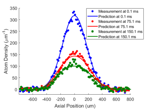
Figure S3: Measurements and predictions (Eq. S38) for the evolution of the axial profiles in a mixture. The magnetic field is tuned so that $a_{S}=15\,a_{0}$. The two-body loss rate constant $K_{2}^{a}=2\times 69.0\,\mu{\rm m}^{3}/s$ is determined from the fit of $N(t)$, Eq. S30 to the data.

To prepare the sample, a 50-50 incoherent mixture of atoms in spin states $|\uparrow_{z}\rangle$ and $|\downarrow_{z}\rangle$ undergoes forced evaporation at 300 G. Then the magnetic field is then swept upward to the magnetic field of interest in the weakly-interacting regime. This method avoids the formation of Feshbach molecules and subsequent loss. However, the efficiency of evaporation performed at 300 G, where the elastic scattering cross section is small, is reduced compared to that of the unitary gas at 832.2 G. For this reason, the samples used to measure $K_{2}^{a}$ are at a higher temperature than for the coherently prepared samples. We assume that $K_{2}^{a}$ is temperature independent, as $K_{2}^{a}$ is expected to exhibit a weak momentum dependence in the weakly interacting regime. At the magnetic field of interest, the loss-inducing optical field is applied, and the total number of atoms is measured as a function of time. The optical resonance frequency is determined by finding the peak loss point at each magnetic field of interest. Using the measured initial axial width and the initial radial width deduced from the ratio of the trap frequencies, the initial density profile is determined and Eq. S28 is used to find $K_{2}^{a}$. This procedure is repeated for each scattering length $a_{S}$ employed in the experiments.

We determine the temperature from a fit of a Maxwell-Boltzmann distribution to the spatial profiles, $k_{B}T=m\omega_{x}^{2}\sigma_{x}^{2}/2$, where $\sigma_{x}$ is the fitted Gaussian width. For 15 $a_{0}$, this procedure gives $T=0.56\,T_{F}$, where $T_{F}=0.79\,\mu$K is determined by

$$T_{F}=\frac{\hbar}{k_{B}}(3N\omega_{\rho}^{2}\omega_{x})^{1/3}.$$ (S37)

Note that we have used a factor $3=6/2$ in place of the factor 6 in Eq. S35, as a 50-50 mixture has half of the total number of atoms $N$ in each spin state.

Measurements of $N(t)$ in 50-50 mixtures are shown in Fig. S4 for all of the scattering lengths of interest, using Eq. S30 to determine $K_{2}^{a}$. The values extracted from the fit are displayed in Table 1, where the uncertainty $\sigma_{K_{2}^{a}}$ is determined from the square root of the covariance matrix of the fit (note that this neglects the uncertainty in the initial density). The measured value of $K_{2}^{a}$ changes by $\simeq 10$% as the scattering length is varied, most likely due to changes in the optical detuning and alignment from run-to-run. Note that the axial widths are smaller for the measurements at 0 and 10 $a_{0}$ than for 5, 15, and 24 $a_{0}$. The difference arises from the difference between the trap depths used for 0 and 10 $a_{0}$, where the trap frequencies were $\omega_{\rho}=2\pi\times 1075$ Hz and $\,\omega_{x}=2\pi\times 34$ Hz. The 5, 15, and 24 $a_{0}$ data employed the smaller trap frequencies given in § E.1. The faster timescales of loss for the 0 and 10 $a_{0}$ measurements reflect the higher density of the sample in the deeper trap.

Eq. S29 also predicts the time-dependent axial profiles $n_{1\text{D}}(x,t)$, which can be compared to measurements. For the Maxwell-Boltzmann distribution of Eq. S36,

$$n_{1\text{D}}(x,t)=\int d\rho\,2\pi\rho\,n(\mathbf{r,t})=\frac{4\pi\sigma_{\rho}^{2}}{K_{2}^{a}t}\,\text{ln}\left[1+\frac{K_{2}^{a}t}{4\pi\sigma_{\rho}^{2}}\frac{N(0)}{\sigma_{x}\sqrt{\pi}}e^{-(x/\sigma_{x})^{2}}\right].$$ (S38)

In the limit $K_{2}^{a}t\rightarrow 0$, $n_{1\text{D}}(x,t)$ approaches a 1D gaussian distribution normalized to the initial total atom number $N(0)$, as it should. Using the $K_{2}^{a}$ determined from the fit to $N(t)$, we find that the predicted axial profiles are in quantitative agreement with the measured profiles, as shown for $a_{S}=15\,a_{0}$ in Fig. S3.

Table 1: Two-body loss coefficients.

$a_{S}$ ($a_{0}$)	$K_{2}^{a}$ ($\mu$m3/s)	$\sigma_{K_{2}^{a}}$ ($\mu$m3/s)
0	115	5
5	120	11.6
10	110	6.8
15	138	10
24	136	10

If the measurements in Table 1 are used in the energy-dependent loss rate coefficient $K(E,E^{\prime},t)$ of Eq. S14, however, the loss model does not agree with the measurements in the energy lattice. To obtain quantitative agreement between predictions and data for coherently prepared samples (as is shown in Fig. 2 and 3 in the main paper), we must divide the values of $K_{2}^{a}$ measured in the mixture by two. It is possible that we have incorrectly extracted $K_{2}^{a}$ by using Eq. S27 or Eq. S28.

To gather evidence as to whether or not the factor of 1/2 is correct, we can compare the values of $K_{2}^{a}$ used to fit the coherently prepared sample in Fig. 3 of the main text to predictions for the optically-induced loss rate constant in ⁶Li. We take $K_{2}^{\rm calc}=-2\times\frac{8\pi\hbar}{m}\,a^{\prime\prime}$, where $a^{\prime\prime}<0$ is determined from the complex light-induced phase shift $\phi$ using $\tan\phi=-ik\,a^{\prime\prime}$ at the optical resonance. Here, $\hbar k$ is the relative momentum, and we assume $|k\,a^{\prime\prime}|<<1$ as is the case for our experiments. Note that a factor of two is included to be consistent with the antisymmetrized hyperfine state of Eq. S9 that defines $K_{2}^{a}$, which in turn requires a symmetric spatial state with a total cross section [24] $\sigma_{\rm tot}=8\pi/k\,Im\{f(0)\}$ and an elastic cross section $\sigma_{\rm el}=8\pi\,|f|^{2}$, with $f$ the s-wave scattering amplitude. The corresponding inelastic cross section $\sigma_{\rm inel}=\sigma_{\rm tot}-\sigma_{\rm el}=2\times\frac{\pi}{k^{2}}(1-|e^{2i\phi}|^{2})$ is twice that of Ref. [3], where the scattering atoms were treated as distinguishable and a factor $4\pi$ was used in the cross sections. The supplementary material of Ref. [3] determines $a^{\prime\prime}$ using $x=k|a_{bg}|$ and $\tilde{\Delta}_{0}=(B-B_{\infty})/\Delta B=-1$ in Eq. S5, which gives $L(\tilde{\Delta}_{0},x)\simeq 1$ in Eq. S8 of Ref. [3], yielding

$$K^{\rm calc}_{2}=2\times\frac{8\pi\hbar\,|a_{bg}|}{m}\,\frac{\hbar\,\gamma_{e}}{4\,\mu_{B}\Delta B}\,\,\tilde{\Omega}_{1}^{2}\,,$$ (S39)

where $\tilde{\Omega}_{1}\equiv\Omega_{1}/\gamma_{e}$. With the parameters of Ref. [25], $a_{bg}=-1405\,a_{0}$, $\Delta B=300$ G, and $\mu_{B}/\hbar=2\pi\times 1.4$ MHz/G, $\gamma_{e}=2\pi\times 11.8$ MHz we find $K^{\rm calc}_{2}=277.4\,\mu{\rm m}^{3}/s\,\,\tilde{\Omega}_{1}^{2}$, which gives $K^{\rm calc}_{2}=69.4\,\mu{\rm m}^{3}/s$ at $\tilde{\Omega}_{1}=0.5$ as used in the measurements. This result is in good agreement with the value $K_{2}^{a}=69\,\mu{\rm m}^{3}/s$ that fits the decay of the coherently prepared sample at $15\,a_{0}$, but is, however, half the value $K_{2}^{a}=138\,\mu{\rm m}^{3}/s$ extracted from measurements in the 50-50 mixture using Eq. S28 as noted above. At present, we are unable to resolve this discrepancy, which may arise from applying Eq. S28 to a very weakly interacting mixture or from an incorrect choice of the incoming two-atom state in deriving Eq. S28.

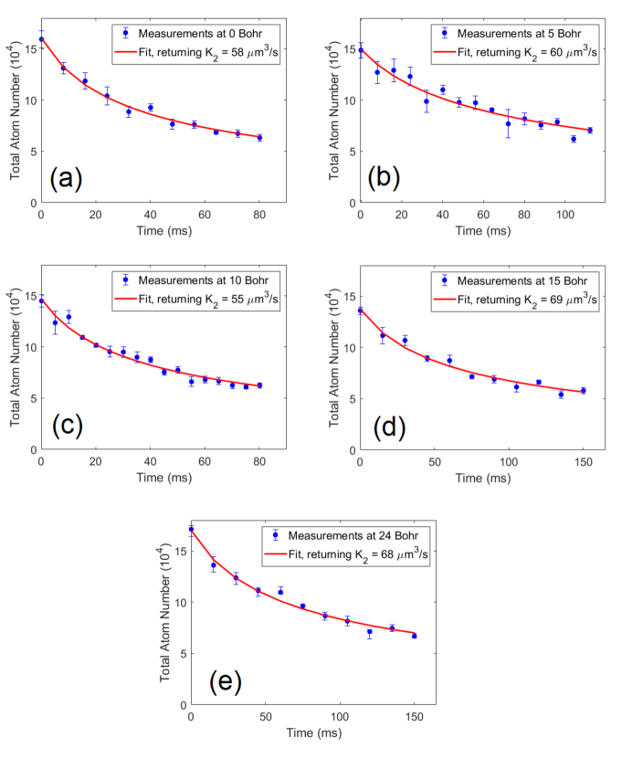
Figure S4: Measurements and predictions of loss in the 50-50 mixture at each scattering length. Different trap depths were used for 0 and 10 Bohr ($\omega_{\rho}=2\pi\times 1075$ Hz, $\,\omega_{x}=2\pi\times 34$ Hz) than for 5, 15, and 24 Bohr ($\omega_{\rho}=2\pi\times 675$ Hz, $\,\omega_{x}=2\pi\times 23$ Hz). (a) Loss at 0 Bohr, with an initial gaussian width 213 $\mu$m; (b) loss at 5 Bohr, with an initial gaussian width 241 $\mu$m; (c) loss at 10 Bohr, with an initial gaussian width 211 $\mu$m; (d) loss at 15 Bohr, with an initial gaussian width 243 $\mu$m; (e) loss at 24 Bohr, with an initial gaussian width 260 $\mu$m.

References

- Bauer et al. [2009] D. Bauer, M. Lettner, C. Vo, G. Rempe, and S. Dürr, Control of a magnetic Feshbach resonance with laser light, Nature Physics 5, 339–342 (2009).
- Wu and Thomas [2012a] H. Wu and J. E. Thomas, Optical control of Feshbach resonances in Fermi gases using molecular dark states, Phys. Rev. Lett. 108, 010401 (2012a).
- Jagannathan et al. [2016] A. Jagannathan, N. Arunkumar, J. A. Joseph, and J. E. Thomas, Optical control of magnetic Feshbach resonances by closed-channel electromagnetically induced transparency, Phys. Rev. Lett. 116, 075301 (2016).
- Arunkumar et al. [2019] N. Arunkumar, A. Jagannathan, and J. E. Thomas, Designer spatial control of interactions in ultracold gases, Phys. Rev. Lett. 122, 040405 (2019).
- Hazzard and Gadway [2023] K. Hazzard and B. Gadway, Synthetic dimensions, Physics Today 76(4), 62 (2023).
- Du et al. [2009] X. Du, Y. Zhang, J. Petricka, and J. E. Thomas, Controlling spin current in a trapped Fermi gas, Phys. Rev. Lett. 103, 010401 (2009).
- Ebling et al. [2011] U. Ebling, A. Eckardt, and M. Lewenstein, Spin segregation via dynamically induced long-range interactions in a system of ultracold fermions, Phys. Rev. A 84, 063607 (2011).
- Pegahan et al. [2019] S. Pegahan, J. Kangara, I. Arakelyan, and J. E. Thomas, Spin-energy correlation in degenerate weakly interacting Fermi gases, Phys. Rev. A 99, 063620 (2019).
- Piéchon et al. [2009] F. Piéchon, J. N. Fuchs, and F. Laloë, Cumulative identical spin rotation effects in collisionless trapped atomic gases, Phys. Rev. Lett. 102, 215301 (2009).
- Natu and Mueller [2009] S. S. Natu and E. J. Mueller, Anomalous spin segregation in a weakly interacting two-component Fermi gas, Phys. Rev. A 79, 051601 (2009).
- Deutsch et al. [2010] C. Deutsch, F. Ramirez-Martinez, C. Lacroûte, F. Reinhard, T. Schneider, J. N. Fuchs, F. Piéchon, F. Laloë, J. Reichel, and P. Rosenbusch, Spin self-rephasing and very long coherence times in a trapped atomic ensemble, Phys. Rev. Lett. 105, 020401 (2010).
- Smale et al. [2019] S. Smale, P. He, B. A. Olsen, K. G. Jackson, H. Sharum, S. Trotzky, J. Marino, A. M. Rey, and J. H. Thywissen, Observation of a transition between dynamical phases in a quantum degenerate Fermi gas, Science Advances 5 (2019), elocation-id: eaax1568.
- Koller et al. [2016] A. P. Koller, M. L. Wall, J. Mundinger, and A. M. Rey, Dynamics of interacting fermions in spin-dependent potentials, Phys. Rev. Lett. 117, 195302 (2016).
- Wall [2020] M. L. Wall, Simulating fermions in spin-dependent potentials with spin models on an energy lattice, Phys. Rev. A 102, 023329 (2020).
- Huang et al. [2023] J. Huang, C. A. Royse, I. Arakelyan, and J. E. Thomas, Verifying a quasiclassical spin model of perturbed quantum rewinding in a Fermi gas, Phys. Rev. A 108, L041304 (2023).
- Huang and Thomas [2023] J. Huang and J. E. Thomas, Decoding transverse spin dynamics by energy-resolved correlation measurement (2023), arXiv:2309.07226 [cond-mat.quant-gas].
- Margalit et al. [2021] Y. Margalit, Y.-K. Lu, F. Çağrı Top, and W. Ketterle, Pauli blocking of light scattering in degenerate fermions, Science 374, 976 (2021).
- Sanner et al. [2021] C. Sanner, L. Sonderhouse, R. B. Hutson, L. Yan, W. R. Milner, and J. Ye, Pauli blocking of atom-light scattering, Science 374, 979 (2021).
- Deb and Kjærgaard [2021] A. B. Deb and N. Kjærgaard, Observation of Pauli blocking in light scattering from quantum degenerate fermions, Science 374, 972 (2021).
- Jannin et al. [2022] R. Jannin, Y. van der Werf, K. Steinebach, H. L. Bethlem, and K. S. E. Eikema, Pauli blocking of stimulated emission in a degenerate Fermi gas, Nature Communications 13, 6479 (2022).
- [21] See the Supplemental Material for a description of the experimental details and of the quasi-classical spin model.
- Wu and Thomas [2012b] H. Wu and J. E. Thomas, Optical control of the scattering length and effective range for magnetically tunable feshbach resonances in ultracold gases, Phys. Rev. A 86, 063625 (2012b).
- Zürn et al. [2013] G. Zürn, T. Lompe, A. N. Wenz, S. Jochim, P. S. Julienne, and J. M. Hutson, Precise characterization of Feshbach resonances using trap-sideband-resolved rf spectroscopy of weakly bound molecules, Phys. Rev. Lett. 110, 135301 (2013).
- Bratten and Hammer [2006] E. Bratten and H.-W. Hammer, Universality in few-body systems with large scattering length (2006), arxiv.org/abs/cond-mat/0410417v3.
- Bartenstein et al. [2005] M. Bartenstein, A. Altmeyer, S. Riedl, R. Geursen, S. Jochim, C. Chin, J. H. Denschlag, R. Grimm, A. Simoni, E. Tiesinga, C. J. Williams, and P. S. Julienne, Precise determination of 6Li cold collision parameters by radio-frequency spectroscopy on weakly bound molecules, Phys. Rev. Lett. 94, 103201 (2005).