A proposal to improve the accuracy of cosmological observables

Abstract

Context. Cosmological observational programs often compare their data not only with $\Lambda$CDM, but also with dark energy (DE) models, whose time-dependent equations of state (EoS) differ from a cosmological constant. We identified a generic issue in the standard procedure of computing the expansion history for models with time-dependent EoS, which leads to bias in the interpretation of the results.

Aims. In order to compute the evolution of models with time-dependent EoS parameter $w$ in a consistent manner, we introduce an enhanced computational procedure, which accounts for the correct choice of initial conditions in the respective backward-in-time and forward-in-time evolution of the equations of motion.

Methods. We implement our enhanced procedure in an amended version of the code CLASS, where we focus on exemplary DE models which are based on the CPL parameterization, studying cases with monotonically increasing and decreasing $w$ over cosmic time.

Results. Our results reveal that a cosmological DE model with a decreasing $w$ of the form $w(a)=-0.9+0.1(1-a)$ could provide a resolution to the Hubble tension problem. Moreover, we find characteristic signatures in the late expansion histories of models, allowing a phenomenological discrimination of DE candidates. Finally, we argue that our enhanced scheme should be implemented as a novel consistency check for cosmological models within current Monte-Carlo-Markov-Chain (MCMC) methods.

Conclusions. Our enhanced computational procedure avoids the interpretational bias to which the standard procedure is unwittingly exposed. As a result, DE models can be better constrained. If implemented into MCMC codes, we expect that our scheme will contribute to providing a significant improvement in the determined accuracy of cosmological model parameters.

1 Introduction

The current cosmological standard model of $\Lambda$CDM is based on many different observations of the Universe on large scales, especially the CMB (see e.g. the balloon-based BOOMERanG experiment by de Bernardis et al. (2000); MacTavish et al. (2006), as well as observations with increasing accuracy by the space missions WMAP (Hinshaw et al. (2013)) and Planck (Planck-collaboration (2018))), the large-scale structure of the cosmic web (see e.g. the Dark Energy Survey (DES) Abbott et al. (2022a), (extended) Baryon Oscillation Spectroscopic Survey (eBOSS/BOSS) Alam et al. (2021), LSST Science Collaboration et al. (2009)), and measurements of the distance ladder using stellar standard candles (see e.g. Perlmutter et al. (1999); Schmidt et al. (1998); Riess et al. (1998); Perlmutter (2003)). However, the model comes with two major conundra, namely the still unknown nature of cold dark matter (CDM) and the nature of the cosmological constant $\Lambda$ which, according to measurements, each contribute roughly 25% and 70%, respectively, to the present-day energy density of the Universe. In attempts to better understand and constrain these components, an accurate measurement of the expansion rate, or Hubble parameter, over cosmic time is desired. Over recent years, discrepancies have been solidified between the measurement of this Hubble parameter at low redshifts $z$, the “local” Hubble constant, and the value of the latter, if high-$z$ data, notably encoded in the CMB, is extrapolated to the present. This issue goes under the header of “Hubble tension (problem)”, and seems to be in conflict with basic assumptions of the $\Lambda$CDM model. In particular, the question arises whether $\Lambda$ should be replaced by a “dark energy” (DE) component, whose energy density and equation of state (EoS) can vary with time, in order to “fit” cosmological observables at various scales. Since the nature of $\Lambda$ has defied a resolution yet, despite theoretical efforts over decades, the Hubble tension adds even more urgency to investigate alternatives in the form of various DE models, which can be tested this way, using ever more precise measurements. Therefore, many cosmological observation campaigns analyze their data, not only in light of testing $\Lambda$CDM, but also to examine the possible signature of DE candidates with a time-varying EoS. Examples include the Dark Energy Survey (DES), see e.g. the Year 3 (DES-Y3) results in (Abbott et al. (2022b)), or the CMB measurements by Planck-collaboration (2018). These and other campaigns often employ a general representation of DE, with a possible time-dependent EoS parameter $w=p/\rho$, where $p$ and $\rho$ constitute a pressure and energy density, in some averaged sense or fluid approach. A useful representation of choice has been the so-called “CPL parameterization” by (Chevallier & Polarski (2001); Linder (2003)) for the EoS parameter,

$$w(a)=w_{0}+\left(1-a\right)w_{a},$$ (1)

which is defined for $a\in[0,1]$, where $a$ is the scale factor of the Friedmann-Lemaître-Robertson-Walker (FLRW) metric of the isotropic and homogenous background universe, while $w_{0}$ and $w_{a}$ are parameters which depend upon the specific DE model. However, in using this form in the comparisons with observations, they are merely free parameters. A cosmological constant $\Lambda$ is recovered as a special case if $w_{0}=-1$ and $w_{a}=0$, i.e. $w_{\Lambda}=-1$ throughout the cosmic evolution.

The CPL parameterization offers a variation of $w$ such that DE models can be studied, which evolve linearly in $a$ from $w\simeq w_{0}+w_{a}$ in the early Universe to $w_{0}$ at the present at $a=1$. Now, campaigns such as Abbott et al. (2022b) and Planck-collaboration (2018) compute from their data the probability distribution of models in the $(w_{0}-w_{a})$-plane (parameter subspace), and they find that the probability of a cosmological constant is within the $1\sigma$ area, “fitted” by a multidimensional Monte Carlo integration to their observational data, using the Markov chain Monte Carlo (”MCMC”) method (see e.g. Carlin & Louis (2008)). While a DE component cannot be definitely ruled out, a cosmological constant is in accordance with both the data in Abbott et al. (2022b) and Planck-collaboration (2018). However, while statistically in agreement with $\Lambda$CDM, it appears that various cosmological observations may prefer different CPL models, in the sense that e.g. the (mean value of the) parameter $w_{a}$ is found to be either positive or negative, as we will discuss. It remains to be seen whether these slight statistical preferences for one or the other eventually converge to a common result, or whether differences pertain, pointing to physical explanations, such as a changing EoS of DE. The work in this paper relates to this question, as follows.

In the computation of the expansion history of the (background) Universe, we identify issues connected to the orders of integrations, and the use of the corresponding initial conditions (ICs) as the starting point of the calculations, in cosmological models having components with time-dependent EoS, i.e. typically a DE component. We discuss the inconsistencies of the standard approach, which does not properly handle the differences in the choice of ICs when performing backward-in-time and forward-in-time integrations of the underlying equations of motion. Since these issues do not arise in models with constant EoS parameters, such as $\Lambda$CDM, they seem to have been overlooked in cases for which time-dependent EoS matter. Therefore, we develop a scheme in order to handle the respective backward and forward evolution consistently, along with introducing a ”bookkeeping” parameter which is flagged according to a given choice of ICs. As a result, and exemplified by our use of the CPL parameterization, we find characteristic signatures of DE models in the late expansion history of the Universe, which allow a phenomenological discrimination of such DE candidates.

In the process, we will also see that the enhanced computational procedure lends itself to the introduction of a novel consistency check of cosmological models. While a modification of the standard MCMC method is beyond the scope of this paper, we will argue that an implementation of the mentioned consistency check within these MCMC methods should be a way to reduce dramatically the available parameter space of models, leading to a significant increase in the determined accuracy of model parameters from such an extended MCMC, in turn. We will describe the steps that would be required to pursue this extension.

This paper is organized as follows. In Sec. 2, we recapitulate the basic equations involved in the evolution of the background universe. In Sec. 3, we illustrate and discuss in qualitative terms the issues that arise in the backward and forward evolution of cosmological models having components with time-dependent EoS, and how to overcome them. In Sec. 4, we present quantitative results for exemplary models with DE, upon implementing our enhanced computational procedure in an amended version of the CLASS code. This way, we can accurately calculate the expansion histories and spectra, and discuss our results in comparison with those of the standard approach. We consider two different CPL-based model universes, one inspired by the mean values of the DES-Y3 results, and an alternative CPL model with positive $w_{a}$ parameter. In light of our findings, we include in Sec. 5 a discussion of the consequences for the Hubble tension problem, and we suggest a multi-step enhancement to be implemented in the standard MCMC routines, in order to increase the determined accuracy of the parameters of cosmological models with DE. A summary and conclusion is presented in Sec 6. The results of additional calculations and consistency checks can be found in two appendices.

2 Basic equations

We start with a recapitulation of the basic equations in the computation of the background evolution of FLRW models, whose observables depend upon cosmic time $t$, or scale factor $a$, but not on spatial coordinates. If we assume that all cosmic components of a given FLRW model can be described as “cosmic fluids”, we can assign in each case (“i”) an equation of state (EOS) which relates the respective energy densities $\rho_{i}$ and pressures $p_{i}$ via the corresponding EoS parameter $w_{i}$,

$$p_{i}(t)=w_{i}(t)\rho_{i}(t).$$ (2)

In general, the EoS parameters $w_{i}$ can themselves change with cosmic time $t$, or scale factor $a$, respectively. However, in the current concordance model of $\Lambda$CDM, all its cosmic components are characterized by a constant, i.e. time-independent $w_{i}$. Applying the first law of thermodynamics to the adiabatic expansion of a comoving volume in the Universe yields the energy conservation equation

$$\frac{\partial\rho_{i}}{\partial t}+3H\left(\rho_{i}+p_{i}\right)=0.$$ (3)

Applying Eq. (2) and assuming that all EOS parameters $w_{i}$ are constant, and that there is no transformation between different components, one arrives at

$$\rho_{i}(a)=\Omega_{i,0}\rho_{\text{crit},0}\>a^{-3(1+w_{i})}.$$ (4)

The factor in front is the (normalized) critical density defined below; the subscript “$0$” customarily refers to present-day values. Thus, under the above assumptions, the evolution of the various $\rho_{i}$ as a function of the scale factor $a$ follows a simple law (the dependence on $t$ is indirect via $a=a(t)$). In the flat $\Lambda$CDM model, we have constant EoS parameters as follows: $w_{r}=1/3$, $w_{b}=0=w_{cdm}$ and $w_{\Lambda}=-1$, i.e. for the energy densities for radiation $\acs{SYMed}_{r}\propto a^{-4}$, for baryons $\acs{SYMed}_{b}\propto a^{-3}$, for CDM $\acs{SYMed}_{cdm}\propto a^{-3}$, and for the cosmological constant $\rho_{\Lambda}\propto a^{0}=const$.

These energy densities enter in the standard procedure of integrating the Friedmann equation

$$\acs{SYMH}^{2}(t)=\frac{8\pi\acs{SYMG}}{3\acs{SYMc}^{2}}\left[\acs{SYMed}_{r}(t)+\acs{SYMed}_{b}(t)+\acs{SYMed}_{\text{CDM}}(t)+\acs{SYMed}_{k}(t)+\acs{SYMed}_{\acs{SYMDE}}(t)\right],$$ (5)

from the early Universe to the present. We include the curvature term in the formula for completeness, but $\rho_{k}$ is set to zero in $\Lambda$CDM, and we will also set $\rho_{k}=0$ in this paper. $H(t)$ is the so-called Hubble parameter (”Hubble function” would be the more correct description, we will use the term “expansion rate” for it interchangeably), defined as

$$H(t)=\frac{\dot{a}}{a},$$ (6)

where the dot denotes the derivative with respect to cosmic time $t$. The criticaldensity is given by

$$\rho_{\text{crit},t}=\frac{3H^{2}(t)c^{2}}{8\pi G}.$$ (7)

The customary density parameters

$$\Omega_{t,i}=\frac{\rho_{i}(t)}{\rho_{\text{crit},t}},$$ (8)

are nothing but the background energy densities, relative to the critical density, whose present-day value is given by

$$\rho_{\text{crit},0}=\frac{3H_{0}^{2}c^{2}}{8\pi G}.$$ (9)

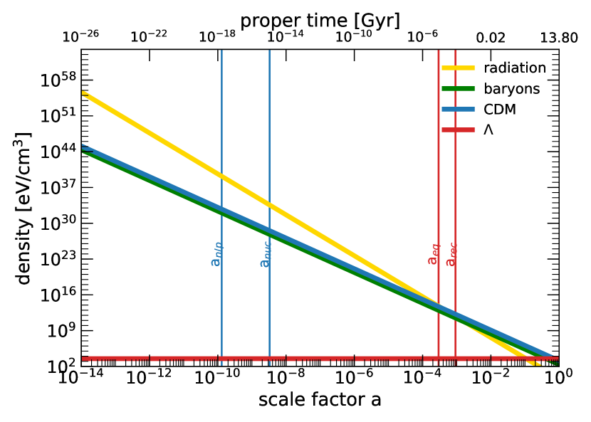
Figure 1: Evolution of energy densities and expansion rate in the $\Lambda$CDM concordance model Top panel: evolution of the energy densities, determined by Eq. (4). Bottom panel: evolution of the expansion rate $H$ in natural units, determined by the total of the energy densities given by Eq. (5). The vertical lines in blue bracket the epoch of big bang nucleosynthesis, between neutron-proton freeze-out at $a_{\text{n/p}}\sim 1.3\cdot 10^{-10}$ and nuclei production $a_{\text{nuc}}\sim 3.3\cdot 10^{-9}$, while the vertical lines in red (at larger scale factor) indicate the time of matter-radiation equality $a_{\text{eq}}$, followed by recombination $a_{\text{rec}}$, in terms of the scale factor $a$.

The Friedmann equation can be alternatively written as an algebraic closure condition, and at the present time it reads

$$1=\Omega_{r,0}+\Omega_{b,0}+\Omega_{\text{CDM},0}+\Omega_{k,0}+\Omega_{\Lambda,0}$$ (10)

(including the curvature term in the formula for completeness). So, we can interpret Eq. (4) as the result of a “backward-in-time integration” (because $\rho_{\text{crit},0}$ depends on $H_{0}$) of the energy conservation equation (3) for the individual components of a given model, as a function of scale factor $a$. This “backward-in-time integration” has to be performed, because we have no equation which determines the initial conditions (ICs) in the early Universe from first principles. However, we do have CMB measurements, which provide us with information of the conditions at place at a redshift of $z\sim 1090$, and using this high-precision data we can infer the present-day values of, say, the $\Lambda$CDM model parameters, if extrapolated to the present. So, Eq. (4) determines the ICs in the early Universe, while customarily performing a “forward-in-time integration” of $H$ when solving the Friedmann equation  (5). Indeed, the specific requirements for integrating consistently the densities for models with cosmic components having time-dependent EOS parameters will be discussed in the next sections.

The observation of the CMB by the Planck mission Planck-collaboration (2018) confirmed previous measurements and more accurately determined the set of parameters of the LCDM concordance model. As an illustration, Figure 1 depicts the evolution of the energy densities of the cosmic components, using the present-day values $\Omega_{r,0}=9.16714\times$10^-5, $\Omega_{b,0}=0.0482754$, $\Omega_{\text{CDM},0}=0.263771$, $\Omega_{\Lambda,0}=0.687762$, and setting $\Omega_{k,0}=0$. The present-day “Hubble constant” $H_{0}=67.56$ km/s/Mpc determines the present-day critical density $\rho_{\text{crit},0}$, which is used in Eq. (4) in order to evolve the densities back in time to the early Universe. The integration of Eq. (5) determines the expansion history and yields an age of $13.8$ Gyr for the Universe in the $\Lambda$CDM model.

3 Cosmic components with a time-dependent EoS parameter: the case for “dark energy”

While the current standard model $\Lambda$CDM is capable of modeling the expansion history of the Universe to good accuracy, certain discrepancies to data have been reported, e.g. with respect to the current value of the Hubble parameter, discussed below. More importantly, the very nature of $\Lambda$ remains an open question, and the community has considered extensions, which include the possibility of a “dark energy” (DE) component, in lieu of $\Lambda$, which exemplifies a time-dependent EoS parameter, the details of which depend on the underlying DE model. As a result, cosmological models are often fit to observational data, which include a DE component having a variable EOS parameter, while the concordance $\Lambda$CDM model with its constant $w_{\Lambda}=-1$ is included as well. Prominent examples of observational campaigns which compare their data to individual DE candidates and a cosmological constant include the CMB observations by Planck-collaboration (2018) and big galaxy surveys such as the Dark Energy Survey Year 3 results (Abbott et al. (2022b)). Both of them use the popular and useful CPL parameterization of Equ.(1). Similarly to the general solution known for a constant EOS parameter

$$\rho\propto a^{-3(1+w_{const})},$$ (11)

the CPL parameterization of DE provides an analytical solution to the integration of the energy conservation equation (3), which reads as

$$\rho\propto a^{3((1+w_{0}+w_{a})\cdot log(1/a)+w_{a}(a-1))}.$$ (12)

This offers a very straightforward way to incorporate CPL-based models of DE into cosmological codes. Unfortunately, a pitfall connected to this simplicity is easily obscured, as we will show in Sec. 4.

Before we present the details, we want to explain the issues that arise in a more illustrative way in this section first. In order to discuss the evolution of the energy density, and its contributing “effect” onto the expansion history, of a component with a time-dependent EOS parameter, we compare it to the evolution of a component with a constant EOS parameter, sketched in Fig. 2.

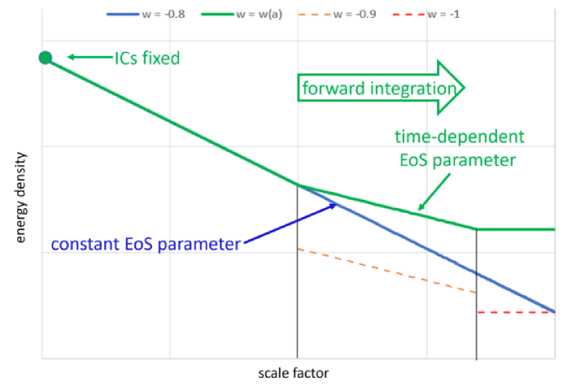
Figure 2: Illustrative comparison between the evolution of energy density for a component with constant or non-constant EoS (arbitrary scaling) The ”blue” component has a constant EOS parameter $w=-0.8$. The ”green” component has a non-constant EOS parameter $w$, which starts out with $w=-0.8$ (equal to the blue component) and evolves in two steps (indicated by the black vertical solid lines) to $w=-0.9$ (the slope is indicated by the dashed orange line) and finally to $w=-1$ (the slope is indicated by the dashed red line). The ”final” density at the present time is higher for the ”green” component.

In this illustration, an exemplary component with a non-constant EOS parameter (green solid line) is compared to a component with constant EOS parameter (blue solid line). The evolution of both components is initiated at identical ICs. For the component with a non-constant EOS parameter, we choose an EOS parameter that drops at two points in time, first from $w=-0.8$ to $w=-0.9$ and finally to $w=-1$, the EOS parameter of a cosmological constant. With each drop, the slope of the energy density evolution flattens (determined by the forward-integration of the energy conservation equation (3)). As a result, the ”final” energy density at the present time is higher, compared to the energy density of the component with constant EOS parameter. Moreover, we recognize that a lower (higher) EOS parameter will decrease (increase) the deceleration of the expansion rate $H$, resulting in an increase (decrease) of $H_{0}$, compared to a component described by a constant EOS parameter with identical ICs in the early Universe.

In contrast, we sketch in Fig. 3 examples of components which each have constant EoS parameter; e.g. the case $w=-1$ describes the $\Lambda$-component in the $\Lambda$CDM model.

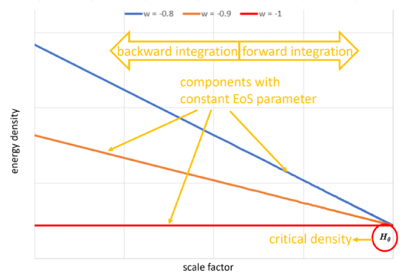
Figure 3: Illustrative evolution of energy densities of components, each with constant EoS (arbitrary scaling): $w=-0.8$ (blue), $w=-0.9$ (orange) and $w=-1$ (red).

No matter what the value for $w$ (blue, orange and red lines), the fact that $w=const$ implies that the order of integration of the energy conservation equation (3) does not impact the final results, as the gradients of the densities never change. We can choose forward-in-time or backward-in-time integration, whatever may be suitable to our problem. In particular, we have this freedom in $\Lambda$CDM, where present-day density parameters $\Omega_{i,0}$ and expansion rate $H_{0}$ can be used in a backward-in-time integration of the energy conservation equation (3) for the energy densities of the individual components via the simplified Eq. (4). In effect, this procedure then determines the ICs in the early Universe, which represent the starting point for the evolution of the background densities, when the forward-in-time integration of the Friedmann equation in (5) is performed. This whole procedure is viable and leads to correct results, as long as all components of a given cosmological model have a constant EOS parameter. However, once we introduce a component with non-constant EoS parameter, such as a DE component in lieu of $\Lambda$, we need to be careful. A component with a non-constant EOS parameter, sketched by the green solid line in Fig. 2, requires a forward-integration of Eq. (3), so we cannot use the customary backward-integration, as applied in the LCDMmodel, in order to compute the evolution of the individual energy densities via Eq. (4). Instead, we must integrate the energy conservation equation (3), starting from the initial densities in the early Universe up to the present, in order to obtain the correct evolution of the densities, which enter the Friedmann equation (5). Related to this careful computation of the backward-/forward-in-time evolution is the choice of the correct starting point(s) of the integrations, as we will elaborate shortly.

Although the Friedmann equation determines the expansion history as the total of the evolution of the energy densities over time (or scale factor) and eventually their initial values, it does of course not explain these initial values. The latter were determined by processes in the (very) early Universe and they impact the subsequent evolution of the background universe ever since, including the values at the present time. Although we cannot compute the ICs from first principles, in practice we can determine (or approximate) them by using observations which provide us with physical information at desirably high redshifts. These are foremost the observations of the CMB, e.g. by Planck-collaboration (2018), providing us with information on the density parameters for the constituents of the Universe at the time when the CMB has formed, i.e. the time of recombination at $z\sim 1090$. Using this data extrapolated to the present, along with the choice of picking $\Lambda$CDM as our concordance model, we end up with a present-day value of the expansion rate of $H_{0}\simeq 67$ km/s/Mpc. We may call it the “concordance value” for $H_{0}$. By applying these parameters of the LCDM concordance model, we can compute the corresponding initial densities, i.e. the “concordance ICs”, now by a backward-in-time integration. So, the evaluation of $H_{0}$ requires two steps. First, measurements of observables refer to a specific cosmic time, e.g. the time when the CMB was emitted. Then, the implication of the measurement is extrapolated to redshift zero which can only be performed by assuming a specific cosmological model, e.g. $\Lambda$CDM. Extrapolated quantities, such as the value of $H_{0}$, are bound to this specific cosmological model, used in the extrapolation. In turn, this “concordance value of $H_{0}$” implies respective “concordance values for the initial energy densities”, and vice versa. We will exemplify the consequences of this for concrete models in Sec. 4. However, it is important to stress that this extrapolation step is not required for direct measurements of $H_{0}$, e.g. in the local Universe. Thus, these measurements are not sensitive to the choice of a specific cosmological model.

Now, the issue of extrapolation becomes critical, once we consider models with time-dependent EOS parameter, such as a DE component, which is often used in the analysis of cosmological observations to examine DE candidates with a time-dependent EOS parameter, and to compare it to a cosmological constant. In this case, the freedom in the order of the integrations, which we have for $\Lambda$CDM, leads to inconsistent results when applied to such models. Therefore, we want to set up a general rule, illustrated in Fig. 4, how to compute the initial energy densities for components with time-dependent EOS parameter via integration of the energy conservation equation (3), in order to solve the Friedmann equation (5), such that the calculations lead to consistent results.

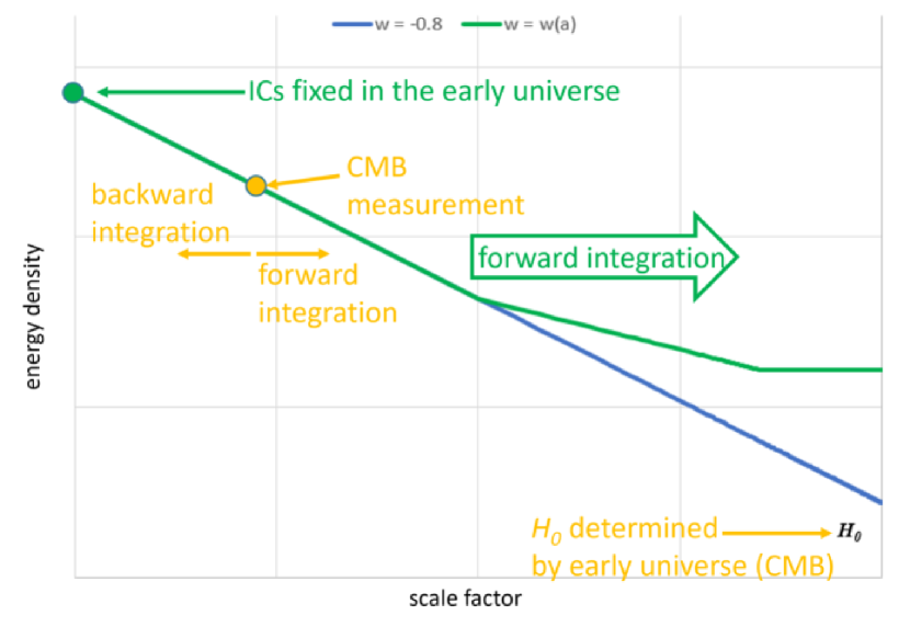
Figure 4: Illustration of integration orders in determining energy densities of cosmic components. The actual IC are fixed by processes in the very early Universe, but we have only access to observables at specific later times (resp. redshifts). The values of the latter determine the value of $H$, and by extrapolation to the present the value of $H_{0}$. If $H_{0}$ determined by the CMB is used, it is this starting point (referred to as ”CMB measurement”) which must be used in the integration of Eq. (3): values for the energy densities before this point in time have to be calculated using backward integration, while values for the energy densities after this point in time have to be calculated using forward integration. The ”green” component has a time-dependent $w$, while the ”blue” component has a constant $w=-0.8$.

For example, when we apply the CMB-based determination of $H_{0}$, it is the time of recombination $a_{\text{rec}}$ (referred to as ”CMB measurement” in the illustration), which shall be the ”starting point” of the integration of Eq. (3): backward integration to get the energy densities before $a_{\text{rec}}$, all the way back to the very early Universe, and forward integration to get the energy densities at all later times past $a_{\text{rec}}$. On the other hand, if we choose a value of $H_{0}$ determined by observations of the local Universe, when we may assume $z\approx 0$, then the starting point is the present, and the integration of the energy densities is performed backward in time.

To elaborate more on these rules for the integration order, which we will adopt in the next section, we present two additional illustrations. The first one depicted in Fig. 5 displays a situation where the recombination time should be our reference point. However, when we apply a standard backward integration, using the present-day value of $H_{0}$ extrapolated from CMB measurements, we arrive at wrong IC, and not the ones which gave actually rise to the CMB which we measure. As a result, even a subsequent correctly performed forward integration of Eq. (3) will result in an incorrect evolution of the expansion history.

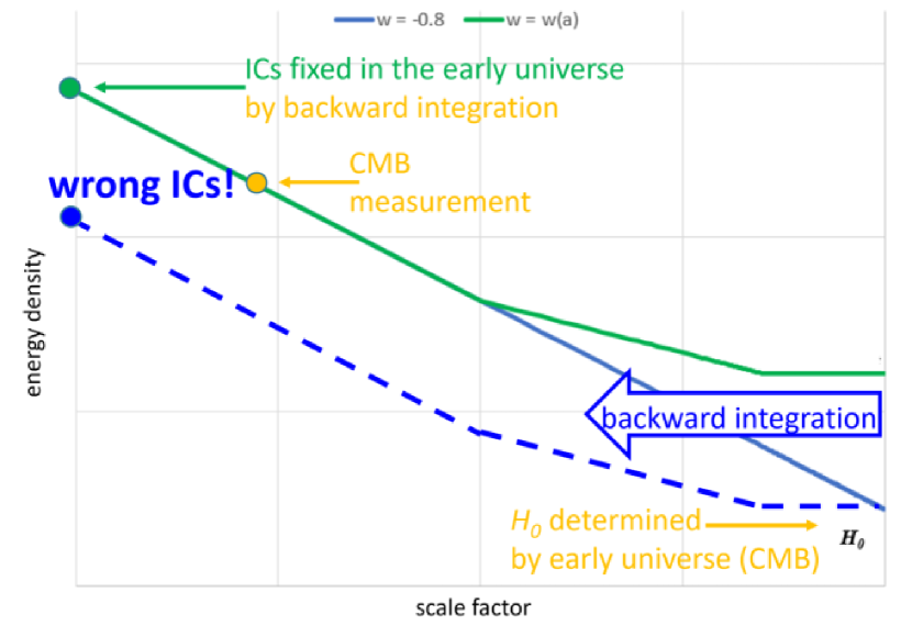
Figure 5: Integration with wrong ICs This illustration complements the one depicted in Fig. 4. The customary backward integration of the component with time-dependent EOS parameter (in blue) leads to incorrect IC, when we start from the value of $H_{0}$ determined from observations of the early Universe.

The second illustration is shown in Fig. 6, and depicts a situation, where the present time is the reference point, using a value of $H_{0}$ determined by observations of the local Universe. (These measurement values of $H_{0}$ typically tend to be higher than those determined by the observation of the CMB, known as the Hubble tension problem, which we will discuss in the next sections).

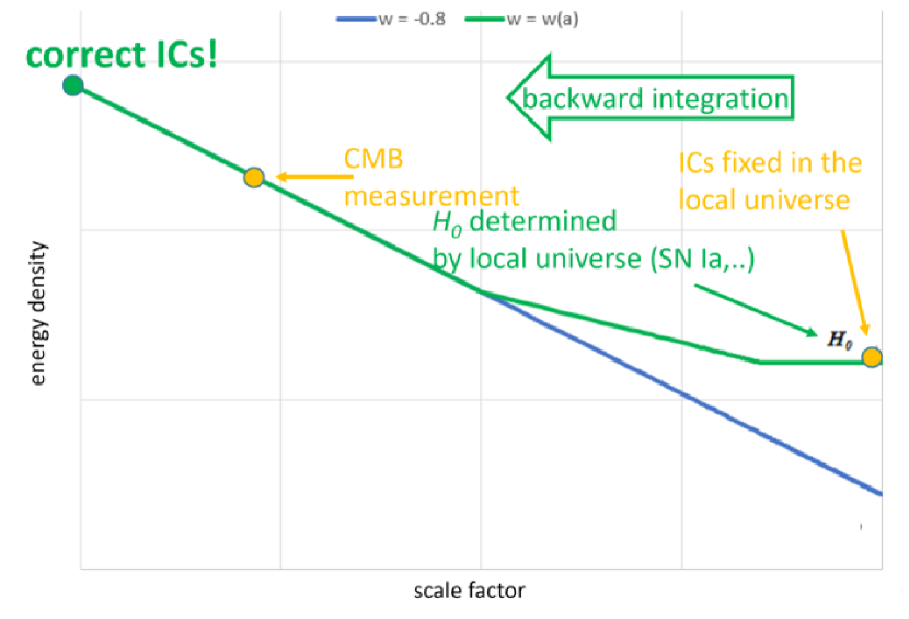
Figure 6: Integration with correct ICs This illustration complements the one depicted in Fig. 4. The customary backward integration of the component with time-dependent EOS parameter (in green) “ends up” at the correct IC, when we start from the value of $H_{0}$ determined from observations of the local Universe.

When we now apply an integration backward in time, we determine the cosmic energy densities in a consistent manner, ending up at the correct IC. A subsequent forward integration will then result in a correct evolution of the expansion history.

In the next section, we will go beyond this qualitative picture and present detailed results for exemplary model universes having a DE component. The enhancements we apply can be summarized as follows.

If the ”early”, CMB-based extrapolation to $H_{0}$ is used:

• computation of the IC with the $\Lambda$CDM concordance parameters

• forward integration, starting at the computed IC

• use of the parameters of the investigated model universe.

If the ”local” value of $H_{0}$ is used:

• backward integration, starting at the given value of $H_{0}$

• use of the parameters of the investigated model universe.

4 Computation of exemplary cosmological models with dark energy

In this section, we will make more precise our procedure, where we suggest to add a novel parameterization, in order to perform the computations of the expansion histories of cosmological models, having components with time-dependent EoS, in a consistent manner. The parameter will serve as a kind of bookkeeper to decide which data (”early” vs. ”local” in cosmic time or scale factor, respectively) determines the configured value of $H_{0}$, in order to perform the correct computations of the IC and integration of Eq. (3).

As already mentioned, “early” values of $H_{0}$ are determined by a two-step procedure. In the first step, we compute the IC, which determined the observations of the configured value $H_{0}$. In doing so, we must apply the same model parameters which were used to extrapolate the observational data to the present-day $H_{0}$, in order to “arrive” at the identical IC, which evolved to those quantities that give rise to the measurement values. Subsequently, we have to integrate the energy densities via the energy conservation equation (3) for each considered component, starting at the computed IC, instead of using Eq. (4), by applying the parameters of the model under consideration, e.g. a model with a dynamical form of DE. Obviously, local measurement values of $H_{0}$ need no extrapolation of observational data to the present-day value of said $H_{0}$. Hence, there are no special requirements on the computation of the IC, but we have to perform a backward integration of Eq. (3), applying the parameters of the model under consideration. In either case, the evolution of the background universe can be rightfully considered as an IVP, determined by the initial energy densities in the early Universe, which give rise to the configured value of $H_{0}$ as determined by (very) high-$z$ or low-$z$ observations, respectively.

While we have emphasized the issue of consistent backward/forward integrations with respect to the adopted measurement value of $H_{0}$ in models with time-dependent EoS, we must also stress another point. As a matter of fact, the data analysis of cosmological observations also often employ variations in the density parameters $\Omega_{i,0}$, e.g. variations in the matter content $\Omega_{m,0}$, which are different from the values of the concordance $\Lambda$CDM model. This sampling of parameters is also related to the adopted routines, typically MCMC methods.

Therefore, in highlighting our proposed procedure, we actually need to consider two different sources of variations in the parameters of a considered model universe: 1) at least one of the components has a time-dependent EOS parameter, as such a component is often used in the data analysis of cosmological observations, typically a DE component, and 2) the density parameters $\Omega_{i,0}$ of components may be different from that model which was used in the extrapolation of $H_{0}$ (i.e. different from the density parameters of the concordance model), as typically encountered in the MCMC data analysis of cosmological observations.

In our paper, we explore the impact of both sources of variations in the computations of model universes. To this end, we use the Boltzmann code CLASS (Cosmic Linear Anisotropy Solving System), which was designed to provide a flexible coding environment for implementing cosmological models, to calculate their background evolution and linear structure formation. The modular concept of CLASS and the coding conventions make it possible to enhance the existing code, without the risk of compromising existing functionality. Furthermore, it offers the configuration of a CPL-based DE component. The underlying code concepts can be found in Lesgourgues (2011), and the code is publicly available at http://class-code.net/. The version used in our paper, the up-to-date version when we started this project, is version 2.9 (21.01.2020). This version uses the “Planck 2018” cosmological parameters from Planck-collaboration (2018) as the default parameter set. Additionally, the configuration provides different sets of precision configuration files, to reflect varying requirements on precision needed in the results and available computation time. The precision configuration offering the highest accuracy is proofed to be in conformance with the Planck results within a $0.01\%$ level.

We developed an amended version of CLASS, which includes our suggested enhancements in the procedure of computing the IC and the integration of the energy densities. The novel parameterization of an early-based (CMB) versus locally determined value of $H_{0}$ makes sure that the corresponding “switch” is carried out in the computation of the IC of the DE component and the subsequent integration of Eq. (3). If the parameter is flagged as “early”, it is assumed that the “concordance LCDM” parameters, i.e. the Planck-based value of $H_{0}$ and all the other model parameters from Planck-collaboration (2018) are used, mentioned in the description of Fig. 1. If the parameter is set to “local”, then the calculation proceeds with the assumption that a locally determined value for $H_{0}$ is being used. We use the CPL-based DE model in CLASS, which includes a cosmological constant as a special case.

We first mention our results, concerning the impact of a variation of the (non-radiation) density parameters on the computation of model universes, in light of the issues of backward/forward integration and the adopted value of $H_{0}$. The bottom line is that we found no significant impact by our improved computational procedure, even for “exotic” models with very different values of $\Omega_{i,0}$, compared to $\Lambda$CDM. Our computational scheme gives results not different from those applying the standard procedure. A marked difference only occurs, if the density parameter of radiation is changed. We relegate these results and their explanation into Appendix A.

However, our investigation of models having components with non-constant EOS parameter, corresponding to the illustrations of the previous section, does reveal differences between our scheme versus the standard customary approach. We exemplify these differences by computing two different model universes with DE in the next two sections.

4.1 A CPL model for DE inspired by the Dark Energy Survey Year 3 Results

In order to examine our suggested procedure, we are interested in probing the scheme for models which differ from the concordance $\Lambda$CDM model, if ever so slightly. We consider first a comparison of the results of DES-Y3 with $\Lambda$CDM, as follows. We stress that DES-Y3 is in accordance with $\Lambda$CDM to within 1-$\sigma$. But they investigated also the CPL model of DE (see Eq. (1)) and find values of $w_{0}=-0.95^{+0.08}_{-0.08}$ and $w_{a}=-0.4^{+0.4}_{-0.3}$. We use the mean values of these parameters to describe a cosmology with DE and call it the “DES-Y3 CPL model” for simplicity. For these CPL mean values, the EoS of DE would evolve from an initial value of $w_{DE}=-1.35$ to a final value of $w_{DE}=-0.95$, i.e. a model with increasing EOS parameter.

4.1.1 Standard procedure (Fig. 7)

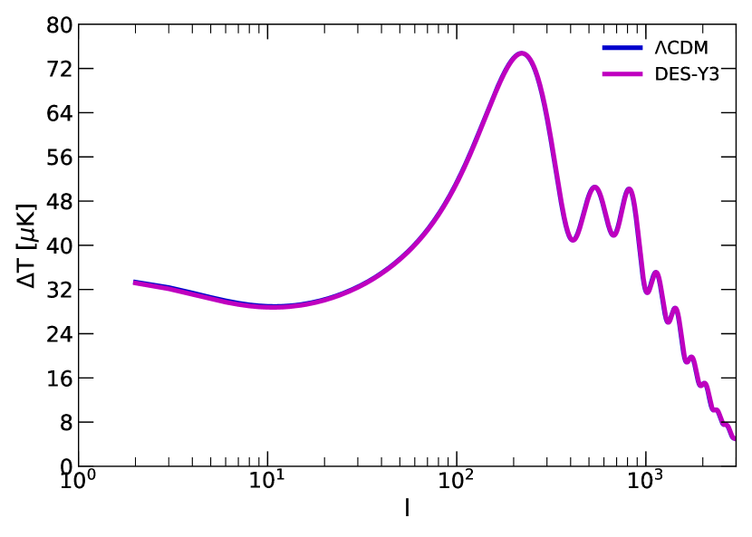
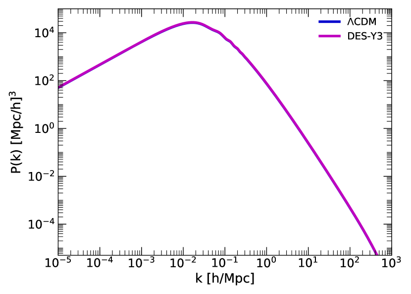
Figure 7: DES-Y3 CPL model with $w_{0}=-0.95$ and $w_{a}=-0.4$ (magenta) and $\Lambda$CDM (blue) both computed with the standard procedure We use the original version of CLASS and the value of $H_{0}$, determined by CMB observations from Planck-collaboration (2018). The top panel displays the expansion history, where the vertical lines in red indicate the time of matter-radiation equality at scale factor $a_{\text{eq}}$, followed by recombination $a_{\text{rec}}$ (both determined by the cosmological model). The bottom part shows the relative deviation of the respective expansion histories (gray curve), which only matters at late times/high scale factors. The middle and bottom panels show the CMB temperature spectrum (temperature anisotropies) as a function of mode number $l$, and the matter power spectrum as a function of wave number $k$, respectively.

We start by showing the expansion history of this “DES-Y3 CPL model”, compared to $\Lambda$CDM, using the standard computational procedure, shown in the top panel of Fig. 7. We used the original code of CLASS with the default value of $H_{0}=67.56\pm 0.42$ km/sec/Mpc, obtained by Planck-collaboration (2018) (see their Table 2, column ”TT,TE,EE+lowE+lensing”, where CLASS additionally uses a best fit to WMAP data). As expected, we see an almost perfect agreement with the evolution of the LCDMmodel, and only at late stages, beginning at $a\sim 10^{-1}$, a decrease in the expansion rate of the CPL model of $\sim 1$% compared to $\Lambda$CDM is seen. It subsequently “overshoots” the expansion rate of $\Lambda$CDM, and finally is forced back (!) to the configured value of $H_{0}$ (see the gray line at the bottom of the panel). Also, the calculation of the CMB temperature spectrum (middle panel) and matter power spectrum (bottom panel) in Fig. 7 displays a perfect agreement with $\Lambda$CDM. Considering the results of Fig. 5, where the standard computational procedure “arrives” at the wrong ICs, one may be surprised to see such a perfect agreement with $\Lambda$CDM. One explanation for the perfect agreement, in expansion history as well as in the spectra, is straightforward and can be illustrated partly with the top panel of Fig. 1, which displays the evolution of the energy densities in $\Lambda$CDM. We recognize the well-known fact that $\Lambda$ remains a very subdominant component well past $a_{\text{rec}}$. Of course, the same is true for the DE component of the “DES-Y3 CPL model”: although its density (not shown) is not a constant line, it is also very much subdominant compared to the other (initial) densities. The late stages of the expansion history display only a minor deviation from $\Lambda$CDM. This seems in contradiction with the expectation from Fig. 2, which predicts a decrease in $H_{0}$. The explanation is that the “wrong” IC are responsible in forcing $H_{0}$ to the configured value of $67.56$ km/sec/Mpc. The spectra are in agreement with $\Lambda$CDM, also thanks to the mistakenly computed expansion history, by “forcing” $H_{0}$ to the configured value. This calculation corresponds to the situation illustrated in Fig. 5.

4.1.2 Amended procedure (Fig. 8)

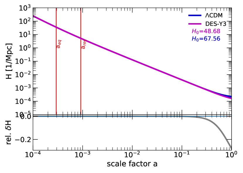
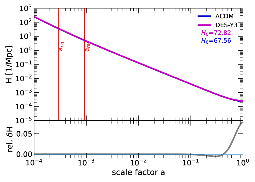
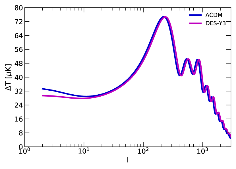
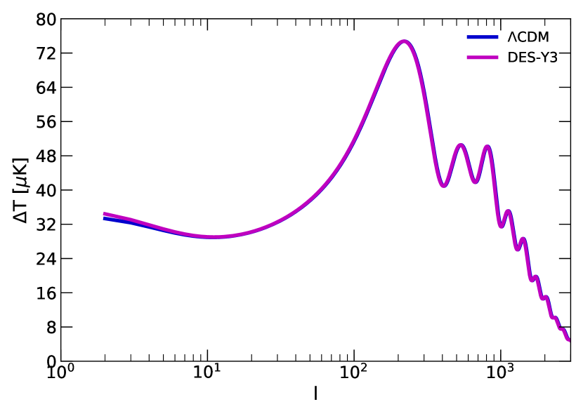
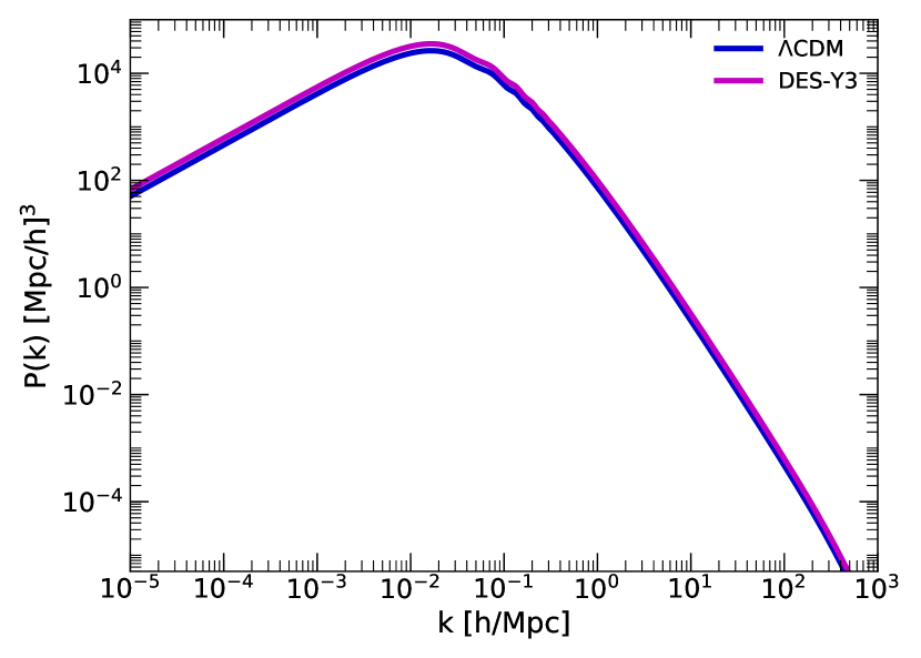
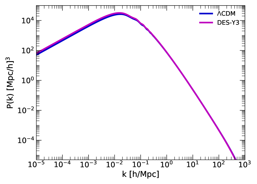
Figure 8: DE component with increasing $w$: the “DES-Y3 CPL model” with $w_{0}=-0.95$ and $w_{a}=-0.4$ (magenta) compared to $\Lambda$CDM (blue), both computed with our scheme Panels on the left-hand column have been computed using the “early” parameterization of $H_{0}=67.56$ km/sec/Mpc using Planck-collaboration (2018), while panels on the right-hand column employ the “local” parameterization of $H_{0}=72.82$ km/sec/Mpc from Riess et al. (2022). Top panels: expansion histories; the vertical lines in red are the same as in Fig. 7. Note the deviations in the expansion histories from $\Lambda$CDM at late times, and the different run of the deviations (see gray curves in the bottom of the top panels). Middle panels: CMB temperature spectra. Bottom panels: matter power spectra. The results based on the CMB-determined $H_{0}$, shown in the left-hand column, display a clear deviation from $\Lambda$CDM, whereas the results based on the locally determined $H_{0}$ are in better agreement with $\Lambda$CDM.

Now, we proceed with the same model comparison, “DES-Y3 CPL model” versus $\Lambda$CDM, but this time applying our proposed computational procedure, which consistently employs the parameterization of $H_{0}$, according to the choice of using “early-based” or “locally-based” values for $H_{0}$. The results are shown in Fig. 8. We make a side-by-side comparison of the plots, where the left-hand column shows results using again the “early” CMB-based $H_{0}=67.56$ km/sec/Mpc from Planck-collaboration (2018), while the right-hand column displays the results using the mean value of the locally-determined $H_{0}=72.82\pm 1.2$ km/sec/Mpc from Riess et al. (2022). Top panels show the expansion histories, and the middle and bottom panels show the CMB temperature and matter power spectra, respectively. Let us first focus on the top panels. The top-left panel depicts the results for the CMB-based value of $H_{0}$. According to the non-positive parameter $w_{a}$ of the CPL model for DE, we clearly see a significantly decreased value of $H_{0}=48.68$ km/sec/Mpc, compared to the configured value $H_{0}=67.56$. Of course, that value for $H_{0}$ is not in agreement with observations, but in light of the expectation from Fig. 2, we can understand what happened: the increasing EOS parameter results in a decrease of $H_{0}$ towards the present time. Again, around $a_{\text{rec}}$, there is no difference between the DES-Y3 CPL model and $\Lambda$CDM, for both $\Lambda$ and DE are then subdominant. The top-right panel shows results for the locally-based value of $H_{0}$, which is parameterized according to the amended version of the CLASS code. The relative evolution of $H$ in the DES-Y3 CPL model displays a slight s-shape (gray line). This calculation corresponds to the situation illustrated in Fig. 6, where the backward integration “arrives” at the correct IC.

The spectra in the left-hand column also display clear deviations from $\Lambda$CDM. While the peak structure in both cases is barely affected, there is an overall shift, horizontally for the CMB spectrum and vertically for the matter power spectrum. More pronounced differences in the spectra occur at large spatial scales (corresponding to low $l$ and low $k$, respectively). Comparing to the right-hand column, which uses the local value of $H_{0}$, we see much better agreement with $\Lambda$CDM for all observables, although some minor deviations in the spectra remain at large spatial scales (probably of no discriminating significance given the error bars of CMB measurements at low $l$). As mentioned earlier, this outcome corresponds to Fig. 6, where the backward-in-time integration “arrives” at the correct IC.

To re-iterate, the simulation run for the early-based (high $z$) value of $H$ employing our scheme does not “force” the expansion rate to the configured concordance value of $H_{0}=67.56$ km/sec/Mpc. Therefore, we see ”exacerbated results” on the left-hand column, compared to the standard procedure depicted in Fig. 7. But in light of the explanations of Fig. 2, we conclude that the results of the amended procedure are correct. Likewise, the results displayed in the right-hand column conform much better to $\Lambda$CDM, because our starting point in the backward integration uses the locally-based $H_{0}$ (at $z\approx 0$), which is “close” to the concordance value of $H_{0}$ to begin with. Nevertheless, the two simulation runs using different $H_{0}$, depending on whether early-based or locally-based measurement values have been used to parameterize the integration runs, do not display consistent results; we see clear differences between the left and right columns in Fig. 8, signaling that backward/forward evolution of the expansion history does not yield consistent results. We will argue in Sec. 5 that the very requirement of recovering consistent results between backward-in-time and forward-in-time evolution of cosmological models should be used in order to extend the standard MCMC procedure to analyze cosmological data. As a result of this requirement, the available parameter space will be significantly reduced, leading to an increase in the accuracy of derived parameters of cosmological models (see also Appendix B).

4.2 A CPL model for DE with a decreasing EoS parameter

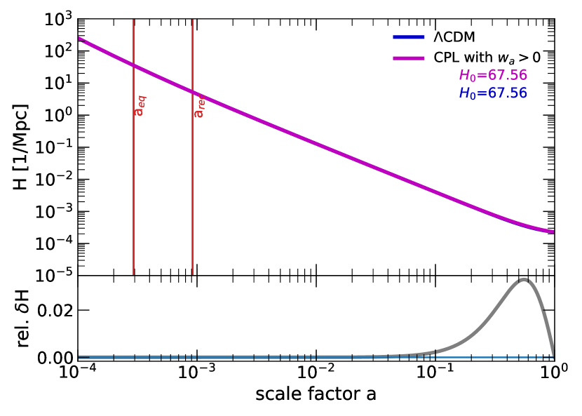
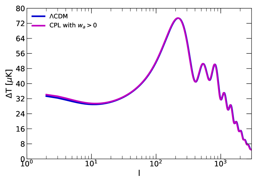
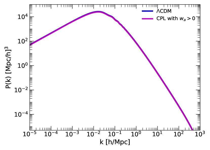
Figure 9: A CPL model with $w_{0}=-0.9$ and $w_{a}=+0.1$ (magenta) and $\Lambda$CDM (blue) both computed with the standard procedure We use the original version of CLASS and the value of $H_{0}$, determined by CMB observations from Planck-collaboration (2018). The top panel displays the expansion history, where the vertical lines in red indicate the time of matter-radiation equality at scale factor $a_{\text{eq}}$, followed by recombination $a_{\text{rec}}$ (both determined by the cosmological model). The bottom part shows the relative deviation of the respective expansion histories (gray curve), which only matters at late times/high scale factors. The middle and bottom panels show the CMB temperature spectrum (temperature anisotropies) as a function of mode number $l$, and the matter power spectrum as a function of wave number $k$, respectively.

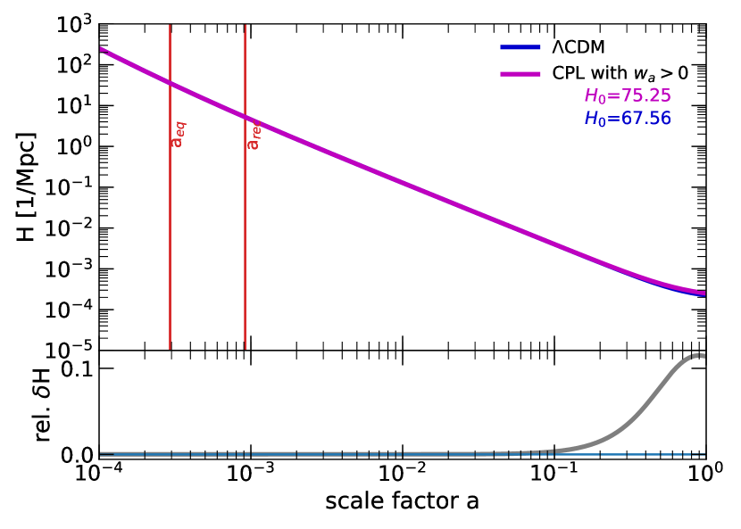
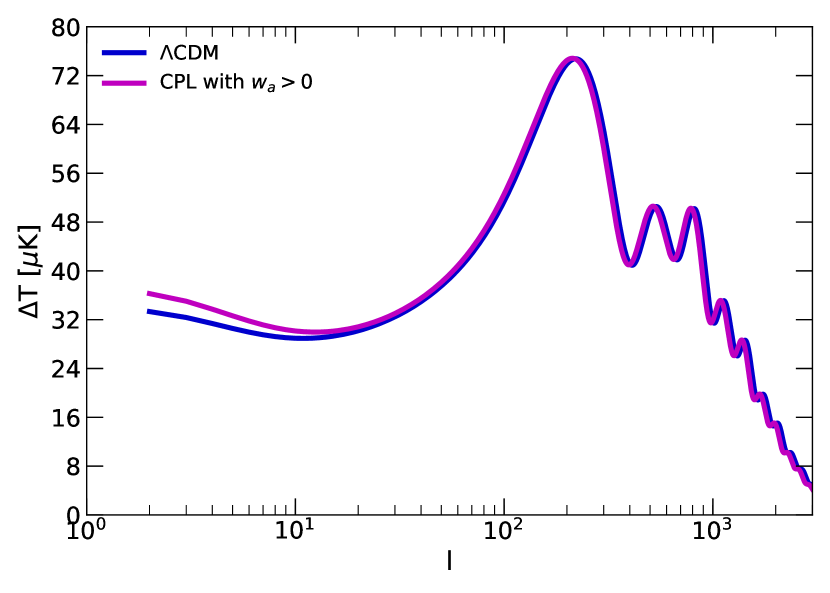
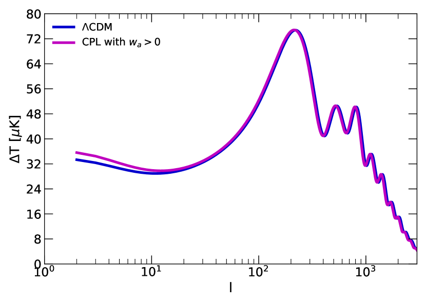
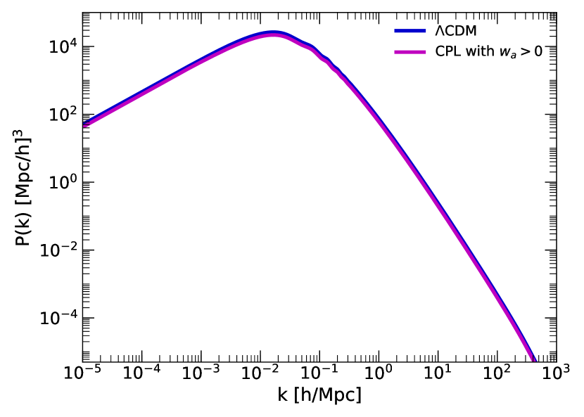
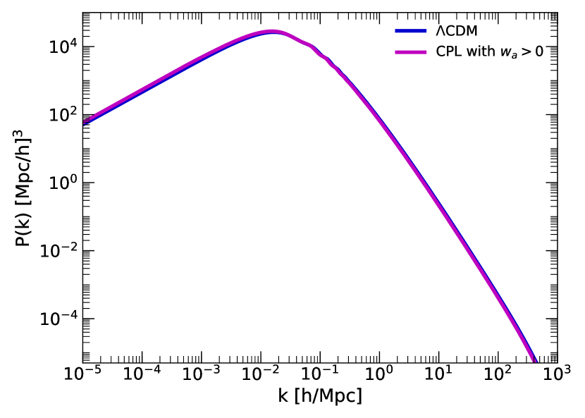
Figure 10: DE component with decreasing $w$: a CPL model with $w_{0}=-0.9$ and $w_{a}=+0.1$ (magenta) compared to $\Lambda$CDM (blue), both computed with our scheme Panels on the left-hand column have been computed using the “early” parameterization of $H_{0}=67.56$ km/sec/Mpc from Planck-collaboration (2018), while panels on the right-hand column employ the “local” parameterization of $H_{0}=72.82$ km/sec/Mpc from Riess et al. (2022). Top row: expansion histories; the vertical lines in red are the same as in Fig. 7. Middle panels: CMB temperature spectra. Bottom panels: matter power spectra. In both columns, we see good overall agreement with $\Lambda$CDM, except for the fact that the chosen CPL model may provide a resolution to the Hubble tension problem. A difference remains in the Hubble constant between left-hand and right-hand columns, see main text.

In the previous section, we considered a CPL-based model of DE whose EoS parameter $w$ increases with time. For this purpose, we took the mean values of the CPL parameters as inferred from the DES-Y3 observations, and considered it as a DE model to compare to $\Lambda$CDM. In this section, we want to study a CPL-based model of DE with decreasing $w$.

While the DES-Y3 and Planck results prefer a non-positive value of the CPL parameter $w_{a}$ clearly below zero (for DES-Y3 see Abbott et al. (2022b) Figure 5 and Figure 4, where they include data from Planck-collaboration (2018) Figure 30), other observations in the more local Universe show a preference for a positive value of $w_{a}$, which would suggest a decreasing $w$ for DE. For example, baryon acoustic oscillations (BAOs) measured in the SDSS Data Release 9 spectroscopic galaxy survey by Anderson et al. (2012), in addition with measurements of luminosity distances from a large sample of SNe Ia by Guy et al. (2010), Conley et al. (2011), Sullivan et al. (2011) yield $w_{0}=-1.17^{+0.13}_{-0.12}$ and $w_{a}=+0.35^{+0.50}_{-0.49}$ (Hinshaw et al. (2013)). Like with DES-Y3, the results are statistically in agreement with $\Lambda$CDM; in the case here a cosmological constant is within the $95$% confidence region in the $w_{0}$-$w_{a}$ plane.

So, given the possibility of discrepant preferences for the CPL parameters of DE from different cosmological observations, we complement in this subsection the analysis of our computational procedure for models with positive value for $w_{a}$.

As a case in point, we use the following CPL parameters, $w_{0}=-0.9$ and $w_{a}=+0.1$, for which the EoS parameter evolves from $w_{DE}=-0.8$ to a present-day value of $w_{DE}=-0.9$. This choice is substantiated by inspection of Figure 5 of the DES-Y3 results in Abbott et al. (2022b), where the green contours in that figure show low-$z$ data alone. For this data, the probability of a cosmological constant is right a the edge of the $1\sigma$-area. Moreover, the centre of this area is such that $w_{0}$ lies below $-1$ and $w_{a}$ is clearly larger than zero, thus also preferring DE over a cosmological constant.

4.2.1 Standard procedure (Fig. 9)

Similarly to Fig. 7 of the model in the previous subsection, we first show in Figure 9 the results for the CPL model with a positive $w_{a}$, using the Planck-based value of $H_{0}$ in the standard procedure. We compare these results from the public version of CLASS with $\Lambda$CDM. The top panel displays the expansion history. We recognize again an almost perfect agreement with $\Lambda$CDM. However, beginning with $a\sim 10^{-1}$, the expansion rate in the CPL model increases to $\sim 3$ % above the value of $\Lambda$CDM at $a\sim 6\times 10^{-1}$, but subsequently is forced back (!) to the configured value of $H_{0}$. Also, we show the CMB temperature spectrum and the matter power spectrum computed with the standard procedure, in the middle and bottom panel, respectively. For reasons mentioned in Sec. 4.1.1, we see an almost perfect agreement with $\Lambda$CDM.

4.2.2 Amended procedure (Fig. 10)

Now, Figure 10 proceeds with the same model comparison, CPL-DE model with $w_{a}>0$ vs. $\Lambda$CDM, but computed by the amended procedure, using “early-based” (left-hand column) and “locally-based” (right-hand column) values for $H_{0}$. In the top panels, we see the expansion history. Again, the expansion rate displays no difference to $\Lambda$CDM around and well past $a_{\text{rec}}$. For the early-based value of $H_{0}$, we see beginning at $a\sim 10^{-1}$ a rise of $H$ resulting in $H_{0}=75.25$ km/s/Mpc, in contrast to the concordance value $H_{0}=67.56$ km/s/Mpc. This result is in agreement with the expectation that a decreasing EOS parameter $w$ leads to a higher Hubble constant at the present. The right-hand panel uses the “local” value of $H_{0}=72.82$ km/sec/Mpc from Riess et al. (2022). As expected and similarly to the right-hand column of the previous Fig. 8, the resulting value of $H_{0}$ is identical to the configured value, as this is the starting point for the backward integration to determine the evolution of the energy densities.

The comparison of the CMB temperature spectra and the matter power spectra obtained from the amended computational procedure, using “early” vs. “local” values of $H_{0}$, with $\Lambda$CDM are also depicted in Fig. 10. For both spectra, we see good agreement with $\Lambda$CDM, except for some deviations at large spatial scales.

Again, the amended code gives us results for the expansion histories, as well as for the spectra, with respect to the different (“local” vs. “early”) parameterizations of $H_{0}$, which are in accordance with the expectations described in Sec. 3.

Moreover, in addition to the above CPL-based DE models, we performed a consistency check, where we use our amended code with a CPL parameterization of the $\Lambda$CDM model, i.e. setting $w_{0}=-1$ and $w_{a}=0$, using the “early” vs. “local” parameterization of $H_{0}$, respectively. Unsurprisingly, we recognize a Hubble tension problem in the “concordance” $\Lambda$CDM model, see Appendix B.

Now, by inspecting the results of the two CPL-based DE models in this section, Fig. 8 vs Fig. 10, we can see that the latter case –a CPL-DE model with $w_{a}>0$, i.e. a decreasing EoS parameter– gives much better agreement with both, the concordance $\Lambda$CDM model and the present-day locally determined Hubble constant from Riess et al. (2022). In other words, backward and forward integrations of this CPL model of Fig. 10 yield results which are (more) consistent with observations, compared to the model in Fig. 8. In principle, we could attribute this finding to the mere chance of having picked favorable CPL parameters (were it not for other reasons which motivated our choice in the first place). Indeed, the CPL parameterization is purely a convenient way of representing DE models, and it is not obvious that any choice of its free parameters will fit perfectly to observations. However, it happens that a choice of $w_{0}=-0.9$ and $w_{a}=+0.1$, upon forward integration, yields a value of $H_{0}=75.25$ km/s/Mpc, which is quite close to the value of Riess et al. (2022) (which is the starting point of the backward integration in each model which we calculated).

We can draw two major conclusions to this section. First, our results suggest that a DE component with a decreasing EOS parameter $w$ may provide a resolution to the Hubble tension problem, because the results of both backward-in-time and forward-in-time integrations, each with their respective $H_{0}$ parameterizations, are in good agreement with the local measurements of $H_{0}$. Second, we argue that the requirement of consistent results between forward and backward evolution of cosmological models should be used as a restrictive criterion of such models. In fact, the procedure can help to find model parameters that are free of the Hubble tension problem, in a very natural way, in that they also provide a present-day Hubble constant in accordance with local measurements. In the next section, we discuss how this approach should be implemented via a three-step procedure in a kind of extended MCMC method, i.e. such that eventually only models without any difference between forward and backward evolution will be sampled. We expect that such an approach will considerably increase the determined accuracy of the parameters of cosmological models.

5 Towards an improvement of the accuracy of cosmological observables

In the previous sections, we discussed the issues connected to the consistent forward-in-time and backward-in-time computations of cosmological models with time-dependent DE component, and how these issues can be avoided by adapting an amended procedure for the self-consistent computation of the expansion history and linear power spectra. In this section, we argue that these proposed enhancements can be and should be employed in the MCMC parameter analysis of models, in order to increase the determined accuracy of model parameters, when compared to observational data. Moreover, in light of the previous findings (see the description of Fig. 10), we re-assess the Hubble tension problem.

The Hubble tension problem basically refers to the discrepancy in the measurement results for $H_{0}$ between observations of the CMB – whose analysis is based on extremely well-understood theories – and observations in the local Universe – based on extremely well-checked measurements. Generally, the latter provide higher values of $H_{0}$ than the CMB-based extrapolated values for $H_{0}$. At the same time, from a theory perspective, we require consistent results for model universes evolved from the early Universe to the present and vice-versa from the present to the early Universe. In Appendix B, we highlight the case of $\Lambda$CDM as an example to check the consistency of cosmological models and their parameters, respectively. This procedure is built on the assumption that the evolution of the background universe is a well-posed IVP, describing the evolution from the early Universe to the present. However, the same shall be true in the converse direction (since we consider the Universe as a ”closed, conservative system”), i.e. using ”ICs” provided by measurements of the local (”present”) Universe, the equations of motion can be evolved backwards-in-time to the early Universe, e.g. to the time of recombination, yielding identical results to the forward evolution.

The question arises how the consistent treatment of the mentioned issue can be combined with the standard approach of comparing cosmological models with data. In general, cosmological observations which apply the MCMC method to explore the parameter space of (typically) FLRW models, and determine the probability distribution of each of the model parameters, by “fitting” the properties of computed model universes to observational data. For example, the data analysis of DES-Y3 matched the computed matter power spectra with observed BAO data, in order to determine the set of model parameters with the highest likelihood. The CMB observation by the Planck mission used a similar procedure: computed temperature spectra were matched with the measured CMB spectrum, yielding the set of model parameters with the highest likelihood, the well-known concordance parameters of the LCDMmodel.

Now, we already emphasized that many observational campaigns (such as DES-Y3, or the Planck mission) include in their analysis (i.e. in their comparison with data) candidates for DE with a time-dependent EoS parameter via a CPL parameterization (see Eq. (1)), along with the cosmological constant of $\Lambda$CDM. Since these candidate models are affected by the issues identified in this paper, we suggest that a novel consistency check is being applied, which avoids these issues. As a result, we expect that the viable parameter set of models shrinks dramatically, such that a significant improvement in the accuracy of determined parameters of cosmological models can be achieved. The standard MCMC computational method should be extended to include a three-step procedure, where each step applies the enhanced computational procedure introduced above, as follows.

First, we remind the reader that, in the standard MCMC method, each of the model parameters is assigned a presumed range of values (known as the priors), which determine the entire parameter space of a given model to be investigated. The parameter space (i.e. a grid of parameter sets) is sampled iteratively, advancing from one parameter set to the next. In each step, the model is computed and matched to observational data. The quality of this match is expressed by computing the “likeliness”, e.g. by a $\chi$-square test. The “likeliness” controls the strategy of the sampler, which also assures not to step out of the defined parameter space but to remain within it. In a final step, the probability distribution (known as the posterior distribution) is computed, applying Bayesian statistics. We propose to extend the computational step for the sampled models to a tree-step procedure.

1. In the first step, the cosmological model under consideration is computed by applying the concordance value for $H_{0}$ and the concordance model parameters. Doing so, we ”accept” the CMB-based ICs of the $\Lambda$CDM concordance model as the “real initial conditions/initial densities” in the early Universe. Starting at these computed ICs, the subsequent forward integration applies the sampled parameter set.

2. In the second step, the resulting value of $H_{0}$ of step one serves as the IC (i.e. this $H_{0}$ is now flagged as ”local”) for a second computation of the sampled model universe, performing a backward integration of the densities, starting from the ”local ICs”.

3. In the final step, the evolution of the densities, i.e. the expansion history and the CMB and matter power spectra from both computations are checked for consistency. Only those parameter sets, which display consistent results, are considered in the subsequent computation of the probability distribution. Since this additional consistency check will lead to a reduction of the allowed parameter space, it will increase significantly the accuracy of the final parameters, resulting from the MCMC analysis.

Encouraged by the results depicted in Fig. 10 for a DE component with decreasing EOS parameter, i.e. $w_{a}>0$ in the specific CPL parameterization, we expect the Hubble tension problem to be explained phenomenologically in a very natural way. While implementing this extension of the MCMC method is outside the scope of this paper, we expect that such an analysis would find $w_{0}>-1$ and $w_{a}>0$, which is in agreement with low-$z$ data depicted by the green contours in Figure 5 of DES-Y3 Abbott et al. (2022b). Also, Y1 results presented in Figure 11.13 of LSST Science Collaboration et al. (2009) depicts a probability distribution in the $(w_{0}-w_{a})$ plane compatible with our expectation.

In contrast, DES-Y3 results (Abbott et al. (2022b)) and the CMB measurements by Planck-collaboration (2018), when comparing a CPL-based model of DE to a cosmological constant, yield a high probability for $w_{a}<0$. Our calculation of an exemplary model in Sec. 4.1 with $w_{a}<0$, where we picked their central values of the CPL parameters calling it ”DES-Y3 CPL model” for mere convenience, does not pass the recommended consistency check. This discrepancy is based on the “miss-fitting” of CPL-based models to observational data in the standard procedure of computing the expansion history, as exemplified in Sec. 4 (see the descriptions of Figs. 9 and 7).

Finally, we stress again that the cosmological model, which is used in deriving extrapolations of observables, such as $H_{0}$, is bound to these values. In other words, the ICs used, $H_{0}$ and the corresponding cosmological model (parameters) are inextricably linked together, where none of them can be used without the other. This fact also explains results of indirect measurements, which (apparently!) seem not to apply CMB-based measurements, and yet yield values of $H_{0}$ close to the Planck concordance value, as seen e.g. in Figure 1 by Di Valentino et al. (2021). Such a case can be seen in Alam et al. (2021), their Table 5 with $H_{0}=67.35\pm 0.97$, based on Big Bang nucleosynthesis (BBN) and BAO data. They apply the MCMC method, while using $\Omega_{r,0}$ from the concordance model (thus, excluding that from the MCMC-sampled parameter space), and assuming a cosmological constant. Hence, these computations as part of the MCMC method arrive at a value of $H_{0}$ close to that of the concordance model (see Appendix A for counter-examples). In this sense, the use of CMB data is implicit in these mentioned cases, due to the relation between the concordance LCDMmodel, $H_{0}$ and the corresponding initial densities, which have been implicitly applied in their model assumptions.

6 Summary and Conclusion

In this paper, we identified and analyzed a critical issue in the standard procedure of computing the evolution of the energy densities in the computation of the expansion history of model universes. This procedure yields inconsistent results for models with cosmic components having time-dependent EoS parameters. The latter are typically DE components on which we focused here. More precisely, we considered the popular CPL parameterization (1) as a way to represent different DE models, and calculated the backward-in-time and forward-in-time cosmic evolution, where we carefully parameterize the ICs which enter the respective calculations, as follows.

We conceived an enhanced procedure to compute the evolution of the energy densities, in that we implemented a case distinction which provides to the calculation the correct ICs, i.e. the provided $H_{0}$ from measurements based either on the ”early Universe” (”CMB-based”), or the ”local Universe” (based on standard candles). Most important is the correct computation of the initial densities in the early Universe as the starting point for the subsequent integration of the energy conservation equation (3). Hence, for ”early-based” values of $H_{0}$, the required forward-in-time integration starts at the computed initial densities, whereas for ”locally-based” values of $H_{0}$ the integration is performed backward in time. Our procedure presumes that the evolution of the background universe is a well-posed IVP, describing the evolution from the early Universe to the present, and vice versa, according to the basic assumption that our Universe is a closed, conservative system.

We used the enhanced procedure to compute two exemplary cosmological models with a DE component, one with an increasing and the other one with a decreasing EoS parameter $w=w(a)$. We found that the latter model with $w(a)=-0.9+0.1(1-a)$ comes close not only to a consistent evolution, with consistent ICs, when backward-in-time and forward-in-time calculations are compared to each other, but it also predicts a present-day value of the Hubble parameter close to that inferred by observations of the local Universe. Thus, such a DE model may provide a resolution to the Hubble tension problem.

In contrast, using the standard computational procedure for time-dependent EoS parameters of DE components, inconsistencies arise, because the evolution of the expansion rate $H$ is “forced” to the configured value of $H_{0}$, which is typically the ”concordance value” measured by the Planck mission (Planck-collaboration (2018)). This inconsistent ”enforcement” results in an incorrect evolution of $H$ in the late stages of the expansion history, obscuring the fact, that a DE component with a decreasing EOS parameter of certain specificity can actually provide an explanation to the Hubble tension problem.

Subsequently to these findings, we argued that this novel consistency check for cosmological models be included in the standard MCMC method, applied in many observational programs to compare dynamical models of DE to a cosmological constant. It boils down to the requirement to sample only those models which exhibit consistent results between forward-in-time and backward-in-time calculations of the cosmic evolution, upon the correct choice of the ICs. Including this recommended consistency check would extend the standard MCMC method, to include a three-step procedure consisting of a calculation of the forward-evolution, followed by a calculation of the backward-evolution with a final consistency check where only consistent parameter sets are considered in the computation of the probability distribution. This final step would then narrow down the parameter space dramatically, increasing significantly the accuracy of the determined model parameters.

The results depicted in Figs. 8, 10 and 13 illustrate well the known fact that CMB observations alone are not very suitable to discriminate individual models of DE: around the recombination time, the expansion history displays simply too few differences from the evolution of the expansion history based on a cosmological constant, despite huge variations in the DE model parameters. However, by the same token, this non-sensitivity provides us with robust information of the initial energy densities predominant in the early Universe. At the other end of the evolution, differences in the late stages of the expansion history provide a tool to discriminate individual DE candidates. As seen by the gray solid line in the Figs. 8, 10 and 13, the deviation in the expansion history from that of a cosmological constant gives a characteristic signature for individual DE candidates. This is a phenomenological approach, but it can put constraints on the evolution of the EoS of DE candidates. On the grounds of these constraints, new models for DE could be developed, in turn, in the future. Of course, we also have to keep in mind that the CPL parameterization is merely a convenient representation, and one could consider a different evolution of the EoS parameter, altogether. Also, some observations may give indications in which direction to go. For instance, hydrodynamical/geometrical models of the cosmic web presented by Icke (1984), Icke & van de Weygaert (1987) and Icke (2001) indicate that its evolution can be modelled by an effective EoS parameter evolving linearly in redshift, rather than in scale factor. The Hubble tension problem has also triggered more proposals with respect to possible DE candidates, e.g. models of ”early dark energy” (EDE), for a review see Poulin et al. (2023). One of the drawbacks of these attempts is that mitigating the Hubble tension problem increases the $\sigma_{8}$ tension. In Rebouças et al. (2023), this was addressed by assuming a modification of EDE with a piecewise-constant EoS parameter, providing a solution to both problems.

The change in the expansion history and growth factor due to a possible DE component belong to the most significant observables which allow to constrain its EoS. Therefore, observations densely sampled in redshift $z$ with high accuracy of the determined Hubble parameter $H$, especially obtained for $z\leq 2$, will be required from ongoing and future observational campaigns to constrain the evolution of the EoS of DE, specifically to detect potentially a decreasing EoS parameter. If statistically significant deviations from a cosmological constant would be found and backed with multiple observations, it would have consequences, not only for a potential resolution of the Hubble tension problem, but more fundamentally for $\Lambda$CDM and its status as the current cosmological standard model. After all, the Hubble tension problem might result because of the assumption of a cosmological constant. As we have shown in this paper, an exemplary cosmological model having a DE component with a decreasing EoS parameter of $w_{0}=-0.9$ and $w_{a}=+0.1$ comes close in fulfilling the new consistency criterion, along with yielding good agreement with the locally-determined Hubble constant. This is in contrast to other DE models. Also, the $\Lambda$CDM concordance model exhibits disagreements. In fact, demanding the proposed consistency check seems to “rule out” a cosmological constant, see also Appendix B, if we accept the Hubble tension problem as real. In light of our results, we thus argued that the Hubble tension problem might be resolved, once the assumption of a cosmological constant is abandoned in favour of a DE component with a decreasing EOS parameter of certain specificity. Of course, in order to test such a DE model more carefully (also beyond the CPL parameterization), high-accuracy determinations of the Hubble parameter over a range in redshift are required, as just emphasized. In fact, many ongoing and future large-scale structure surveys are probing DE candidates from low-$z$ to mid-$z$ range by determining a prospective evolution in the EoS parameters. For the reader’s sake, we name some of the most important surveys (no ranking implied), including the:

• Dark Energy Spectroscopic Instrument (DESI) survey, see Seo & Eisenstein (2003): measurement of bright galaxies up to a redshift of $z=0.4$, luminous red galaxies up to $z=1$, emission-line galaxies up to $z=1.6$ and quasars up to $z=3.5+$.

• Dark Energy Survey (DES) (Abbott et al. (2022b, a)) applies gravitational lensing for 319 million objects in the range $z=0.2$ to $1.05$, divided into in six bins.

• Hobby-Eberly Telescope Dark Energy Experiment (HETDEX) observes 1 million Lyman-Alpha emitters at $1.9<z<3.5$, and 1 million OII-emitting galaxies at $z<0.5$ (Hill et al. (2012); Gebhardt et al. (2021)).

• Euclid survey (see e.g. Rhodes & Capak (2019)) uses weak lensing observations of galaxies up to $z\geq 2$, BAOs for $z\geq 0.7$ and local observations out to distances of 5 Mpc. The deep survey primarily targets galaxies at $z>6$, where follow-up observations by the James Webb Space Telescope are envisaged.

• Nancy Grace Roman Space Telescope’s High Latitude Time Domain Survey: measurement of thousands of SNe Ia up to $z=2$, see e.g. Hounsell et al. (2018).

• Vera C. Rubin Observatory, previously referred to as the Large Synoptic Survey Telescope (LSST): measurement of SNe Ia with mean $z\sim 0.45$ to max $z=0.8$, see e.g. Ivezić et al. (2019).

In addition, direct measurements in the ”local” Universe remain very important and promising probes, because they are not sensitive to the specific characteristics of presumed cosmological models, as described by e.g. Kenworthy et al. (2019), Bernal et al. (2016), Riess et al. (2021).

Appendix A The Impact of Variations in the Density Parameters ${\Omega_{i,0}}$

In our study of the impact of a DE component with time-dependent EOS onto the computation of the evolution of its energy density, we have used in this paper the same density parameters as for the LCDM concordance model.

In this appendix, we check our amended code for cases with deviations of the density parameters $\Omega_{i,0}$, compared to the values of $\Lambda$CDM, as a testbed how our modification fares in such situations, and compare the results to those of the standard customary approach. In order to provide hard tests, we consider “exotic” models, but for components with constant EOS parameter.

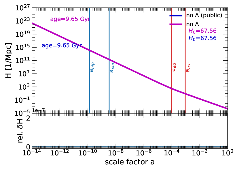
Figure 11: Model without $\Lambda$: The panels display from top to bottom the expansion history, the CMB temperature spectrum and the matter power spectrum of a model universe, which omits $\Lambda$ but increases the CDM component accordingly, such that the total of the energy densities is equal to the critical density (i.e. a case close to the Einstein-de-Sitter model). The blue curves depict the results obtained by the public version of CLASS. The magenta curves show the results from our amended version, which uses the IC of the concordance model. The results of both computations agree very well.

Let us first consider a model without a $\Lambda$-component, while obeying Eq. (10) with vanishing curvature term, i.e. the density parameter for the CDM component is accordingly increased. This case is close to the Einstein-de-Sitter model. The results can be seen in Figure  11, which have been calculated using our amended code as well as the original, public code of CLASS. The expansion histories agree very well, resulting in identical values for $H_{0}$ for both code versions. The same agreement can be seen in the respective power spectra of the model universe. There is only a minor difference of $\sim 10^{-15}$ in the initial densities in the public version, compared to the amended version. We also checked another exotic model, where we modified the density parameters of both baryons and CDM such to make them equal, while leaving the total matter content unchanged. (This model has the same expansion history than $\Lambda$CDM, but the spectra differ.) For both code versions, we get the same results (not shown here).

For both exotic models, the initial densities are not much different, because we changed the matter components and/or $\Omega_{\Lambda}$ which are subdominant in the early Universe. Therefore, we get basically the same results for both codes.

However, once we pick a case where the ICs are greatly affected, we see a difference, which is illustrated by the following model displayed in Fig. 12. Here, we omit $\Lambda$ (as in the case of Figure  11), but additionally we reduce the density parameter for radiation by half, compared to its standard value, while increasing the density parameter for the CDM component accordingly. Since radiation is the dominant component in the early Universe, such an extreme change affects the ICs critically (top panel of Fig. 12). Now, we can see a clear difference between the results from the public and the amended CLASS code in the expansion history, as well as in the spectra. Also, matter-radiation equality $a_{\text{eq}}$ and recombination $a_{\text{rec}}$ are shifted to a later cosmic time, and the present-day expansion rate of $H_{0}=95.54$ km/sec/Mpc, is much higher compared to the configured value of $H_{0}=67.56$ km/sec/Mpc.

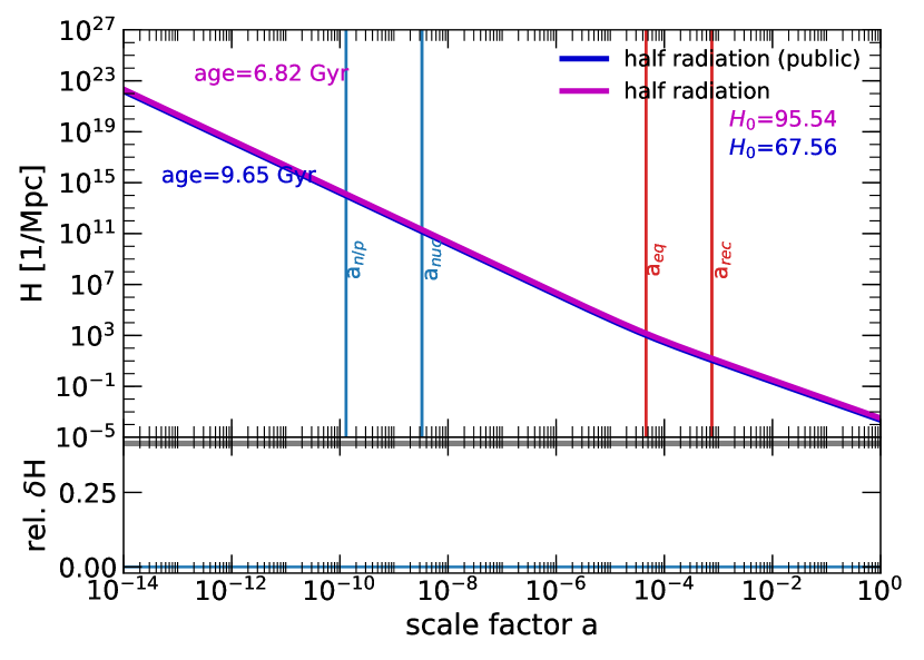
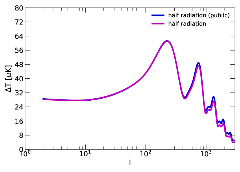
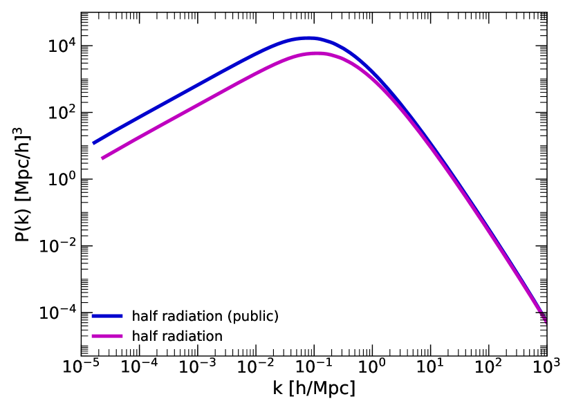
Figure 12: Model without $\Lambda$ and less radiation: The panels display from top to bottom the expansion history, the CMB temperature spectrum and the matter power spectrum of a model universe without $\Lambda$, whose density parameter for radiation is reduced to half its value of the concordance model, while its CDM density parameter has been accordingly increased, such that the total of the energy densities is equal to the critical density. The blue curves depict the results obtained by the public version of CLASS. The magenta curves show the results from the amended version, which uses the IC of the concordance model. The results of both computations significantly deviate from each other.

Of course, the adoption of the concordance ICs, while modifying the density parameter for the radiation component is not in agreement with observations, for both versions of the code. Obviously, this is not a viable procedure in the computation of cosmological models, because it breaks the connection between the ICs and $H_{0}$ established by the concordance model, as we already discussed. In fact, the importance of adopting (keeping) the standard value for the radiation density parameter, especially by excluding it from MCMC parameter space searches, has been known and is handled that way by observational campaigns which apply the standard scheme, see e.g. Abbott et al. (2022b) and Alam et al. (2021). To summarize, provided the density parameter of radiation is the same as in the standard, concordance model, the variation of the remaining parameters leads to the same results for both computational procedures, i.e. for both the public CLASS code and our amended CLASS code.

Appendix B Consistency Check using $\Lambda$CDM

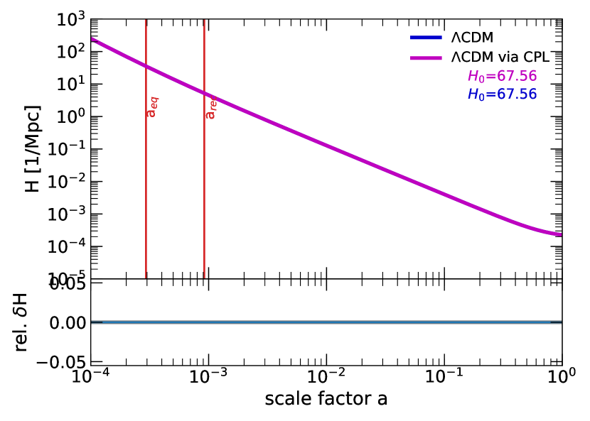
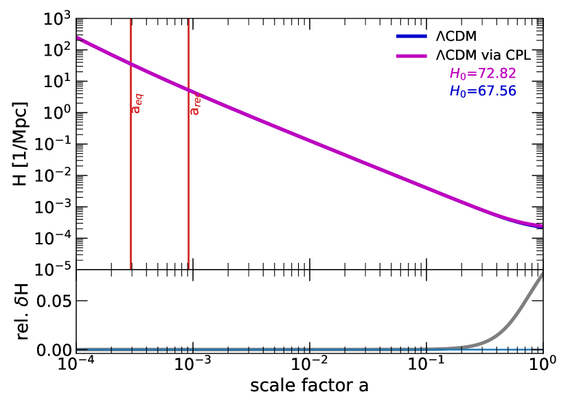
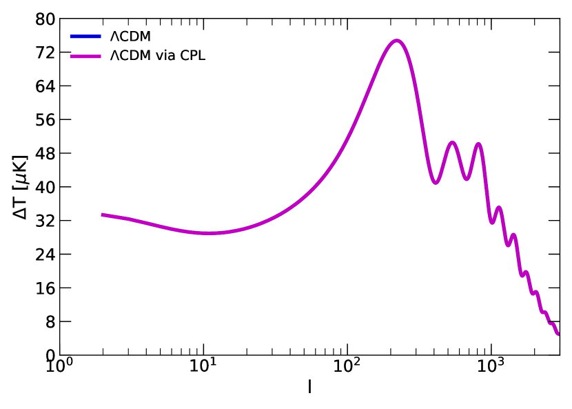
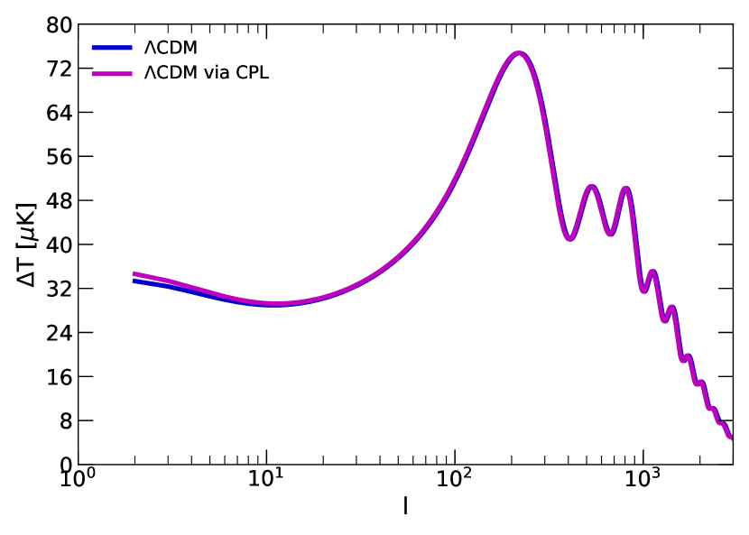
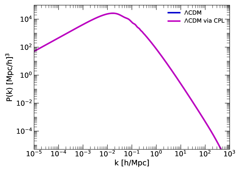
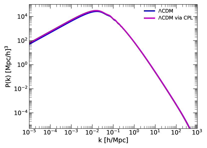
Figure 13: $\Lambda$CDM consistency check We use our amended version of CLASS to compute observables of the LCDMmodel, using the CPL parametrisation with associated parameters $w_{0}=-1$ and $w_{a}=0$. Left-hand panels: calculation based on the parametrisation which uses the “early” CMB-based value of $H_{0}=67.56$ km/sec/Mpc from Planck-collaboration (2018). Since this is equivalent to the standard input in CLASS for $\Lambda$CDM, we see no difference in the results. Right-hand panels: calculation based on the parametrisation which uses the “local” value of $H_{0}=72.82$ km/sec/Mpc from (Riess et al. (2022)). The top row displays the expansion histories, while the middle and bottom rows display the CMB temperature spectra and matter power spectra, respectively. See main text for explanations.

In this appendix, we test our amended CLASS code by computing observables for the $\Lambda$CDM model, and comparing them with the results of the original, public version of CLASS. Our amended code uses the CPL parameterization, i.e. we set $w_{0}=-1$ and $w_{a}=0$ to recover a cosmological constant. We compute two versions, one based on the parametrisation which uses the “early” CMB-based value of $H_{0}$ from Planck-collaboration (2018) (left-hand panels), and another one based on the parametrisation which uses the “local” value of $H_{0}$ from Riess et al. (2022) (right-hand panels). The results and comparison for the expansion histories, as well as for the CMB temperature spectra and matter power spectra, can be found in Fig. 13.

The left-hand panels show no difference in the results, which is expected, since we parameterize the model in a way that is equal to the standard CLASS input for the concordance $\Lambda$CDM model. On the other hand, the right-hand panels show a difference: the expansion history displays similar deviations from the LCDMmodel to those shown in Fig. 10. But the maximum deviation happens at a scale factor of $a=1$, in contrast to Fig. 10, where the maximum deviation is at a scale factor of $a\sim 0.8$. There are also some minor deviations in the spectra in the right-hand panels, limited to large spatial scales. Assuming that the Hubble tension problem is real, we can recognize that $\Lambda$CDM suffers this problem, for the backward and forward evolutions do not yield consistent results. In other words, we see differences in the expansion history (gray curve) from the “concordance model” when we adopt a locally determined $H_{0}$ in our model, see right-hand panel. In this sense, $\Lambda$CDM does not pass the recommended consistency check for cosmological models and their parameters, respectively. Thus, there remains a Hubble tension problem in $\Lambda$CDM.