Neutron-star Measurements in the Multi-messenger Era

Abstract

Neutron stars are compact and dense celestial objects that offer the unique opportunity to explore matter and its interactions under conditions that cannot be reproduced elsewhere in the Universe. Their extreme gravitational, rotational and magnetic energy reservoirs fuel the large variety of their emission, which encompasses all available multi-messenger tracers: electromagnetic and gravitational waves, neutrinos, and cosmic rays. However, accurately measuring global neutron-star properties such as mass, radius, and moment of inertia poses significant challenges. Probing internal characteristics such as the crustal composition or superfluid physics is even more complex. This article provides a comprehensive review of the different methods employed to measure neutron-star characteristics and the level of reliance on theoretical models. Understanding these measurement techniques is crucial for advancing our knowledge of neutron-star physics. We also highlight the importance of employing independent methods and adopting a multi-messenger approach to gather complementary data from various observable phenomena as exemplified by the recent breakthroughs in gravitational-wave astronomy and the landmark detection of a binary neutron-star merger. Consolidating the current state of knowledge on neutron-star measurements will enable an accurate interpretation of the current data and errors, and better planning for future observations and experiments.

1 Introduction

NS are remarkable astrophysical objects for a number of reasons. First, they are incredibly compact, containing a mass of around $1-2\,M_{\odot}$ within a radius of approximately $10-12\,$km. As a result, spacetime within and around these objects is highly curved, often necessitating the use of a strong-gravity framework to model associated phenomena. Additionally, matter inside neutron stars exists under extreme densities, surpassing the nuclear saturation density, $\rho_{0}\approx 2.8\times 10^{14}\,{\rm g}\,{\rm cm}^{-3}$ (the density of atomic nuclei) in their cores. This unique feature makes NSs natural laboratories for investigating matter and strong interactions under conditions that cannot be replicated in controlled terrestrial environments. Furthermore, NSs possess the strongest magnetic fields in the Universe with surface field strengths ranging between $10^{8}\,$ to $10^{15}\,$G. This allows us to also study matter in the ultrahigh magnetic-field regime. Finally, NSs are fast and incredibly stable rotators with rotation periods ranging approximately between $1\,$ms to $10\,$s and some objects rivaling the stability of atomic clocks on Earth.

To employ NSs as cosmic laboratories, it is necessary to measure their macroscopic properties (such as the mass, radius and moment of inertia) and internal features (e.g., the composition of NS crusts and superfluidity). These quantities provide us with a wealth of information about the phenomena occurring in the stars’ interior or in their proximity, allowing us to constrain physics under extreme conditions. However, measuring these properties is inherently challenging, because they cannot be observed directly. Observable quantities often depend on several of these parameters, leading to significant uncertainties and degeneracies in their inferred values. Additionally, the methods used to measure these parameters typically rely on a range of assumptions, introducing varying degrees of model dependence. Therefore, it is of fundamental importance to develop independent methods that target given observables but are based on different assumptions. This will ultimately allow us to improve our knowledge of NSs by comparing and cross-correlating distinct independent measures.

To achieve this objective, a multi-wavelength approach is crucial. By conducting observations across the electromagnetic spectrum, we can explore the diverse population of NSs and gather complementary information about different types of sources. Furthermore, the detection of the first binary neutron star (BNS) merger by the LIGO and Virgo advanced interferometers [1] marked the emergence of gravitational waves as a new messenger for astrophysical studies. The accompanying observation of a short gamma-ray burst (GRB) and a kilonova (KN) [2] reigned in a new era of multi-messenger astronomy, which holds great promise for revolutionizing the study of NSs.

The aim of this review is to provide an overview of the different methods employed to measure NS properties. As fully covering the extensive literature on this topic is beyond the scope of this review, we instead highlight those approaches that we consider most relevant and promising in constraining uncertain NS physics. In particular, we distinguish the messenger and wavelength regime of a certain measurement and assess underlying model dependencies and systematics. This way, we hope to provide the reader with a schematic overview of the different techniques used to study these extreme objects and how reliable these approaches are. We also point out that we purposefully do not aim to summarize current constraints on NS observables. We only mention corresponding estimates sporadically, where we see appropriate, and provide ample references for the interested reader to dive deeper, instead putting our primary focus on the methodology itself.

The review is organized as follows: In Sec. 2, we summarize the state of the art of our NS knowledge, focusing in particular on the description of the different subpopulations of NSs (Sec. 2.1) and our current understanding of their internal structure (Sec. 2.2). In Sec. 3, we discuss the different methods used to measure NS parameters. We focus specifically on the mass (Sec. 3.1), radius (Sec. 3.2), moment of inertia (Sec. 3.3), tidal deformability (Sec. 3.4), compactness (Sec. 3.5), magnetic field (Sec. 3.6), crustal physics (Sec. 3.7), superfluidity (Sec. 3.8) and then touch on a few additional measurements (Sec. 3.9). Finally, in Sec. 4, we provide a summary and discuss conclusions.

2 State of the art

In this section, we summarize our current knowledge of NSs. We start by illustrating the different populations of NSs, describing their most important characteristics. We then review our current understanding of the internal NS structure. Our aim here is not to provide a comprehensive and detailed description of the topic but rather introduce the reader to the general context required to better understand the following sections. For those interested in delving deeper, we refer to dedicated reviews that provide more comprehensive information on the subject matter.

2.1 Neutron-star diversity

The idea of a NS was first proposed just a few years after the neutron’s discovery in 1932. Several physicists suggested that the supernova explosion of a massive star could signal a transition from a normal star to a compact, highly magnetic, rapidly rotating star composed mainly (but not solely) of neutrons [3, 5]. It took some 30 years to confirm this notion, when in 1967 Jocelyn Bell Burnell and Antony Hewish discovered the first NS by spotting its beamed radio emission as a repeating signal, the first pulsar, in their radio telescope [6]. Since then, many more NSs have been discovered and to date more than three thousand are known in different systems and environments: isolated or in binary systems with a large variety of companions, in double NS systems, in the Galactic disk, in Globular clusters, and in nearby Galaxies [7].

In Fig. 1, we present the $P-\dot{P}$ diagram of the known pulsar population, where $P$ denotes the spin period of a NS and $\dot{P}$ its time derivative obtained through pulsar timing. Knowledge of $P$ and $\dot{P}$, in turn, allows an estimate of the NS’s so-called characteristic age, $\tau_{\rm c}=P/2\dot{P}$, if the star spins down due to magnetic dipole radiation, and the surface dipolar magnetic-field strength, $B_{\rm dip}$, (see Sec. 3.6.1 for details). Although the observed NS population is dominated by radio pulsars, several extreme and puzzling sub-classes of NSs have been discovered in the last decades. These include Rotating Radio Transients, magnetars, X-ray Dim Isolated Neutron Stars, Central Compact Objects, and the more common X-ray NSs in binary systems accreting material from a low-mass or high-mass companion star. Despite being presumably governed by a single equation of state (EOS), NSs manifest a surprising observational diversity, which we are only just starting to understand. Moreover, the Galactic core-collapse supernova rate is unable to accommodate the formation of these different NS classes individually [8], suggesting evolutionary links between them [9, 10, 11]. We briefly summarize these different classes here.

Rotation-powered pulsars: With thousands of objects (see dots in Fig. 1), the largest NS class is powered by their rotational energy reservoirs, $E_{\rm rot}$, with braking due to their dipolar magnetic fields (Sec. 3.6.1) supplying luminosities of the order of $L_{\rm rot}\sim|\dot{E}_{\rm rot}|=4\pi^{2}I_{\rm NS}\dot{P}/P^{3}\approx 3.95\times 10^{31}\,{\rm erg}\,{\rm s}^{-1}$ for a fiducial NS moment of inertia, $I_{\rm NS}$, of $10^{45}\,{\rm g}\,{\rm cm}^{2}$, $P=1\,{\rm s}$ and $\dot{P}=10^{-15}\,{\rm s}\,{\rm s}^{-1}$. Although emitting pulsed emission across the electromagnetic spectrum, these sources are typically observed in the radio band (see [12] for a comprehensive overview). The key ingredient to activate this emission is the acceleration of charged particles, which are extracted from the star’s surface by an electrical voltage gap [13, 14]. Moreover, all isolated pulsar periods increase with time, implying a decay in their spin frequencies. Specifically, pulsars are born with fast rotation and high magnetic fields (top left in the $P-\dot{P}$ diagram 1) and evolve towards slower rotation and lower magnetic fields (bottom right). The exact trajectory and timescale differs from pulsar to pulsar and depends on their birth properties and details of the magnetic-field evolution [15].

Rotating Radio Transients: RRATs were discovered as bright ($0.1-3\,$Jy), short ($2-30\,$ms) radio bursts that recurred randomly about every $4\,$min$\,-\,3\,$hr [16]. A study of the arrival times of these bursts led to the discovery of common periodicities, which are interpreted as the rotational periods of underlying pulsars. Instead of constituting their own class, RRATs are now considered an extreme form of rotation powered-pulsars that exhibit extended periods of so-called nulling, i.e., long phases where the regular emission is switched off are interspersed with irregular, sporadic emission of radio pulses (see [17] for a review). Although it has been estimated that RRATs are as numerous as the radio pulsar population [16, 8], these sources are much harder to detect and classify because of their irregularity. [18], e.g., present a catalog of 115 RRATs of which two thirds have $P$ and one third $\dot{P}$ measurements (see diamonds in Fig. 1).

Magnetars: These few dozen, young objects (see stars in Fig. 1) with spin periods between $0.3-12\,$s and inferred dipole magnetic field strengths of the order of $10^{14}-10^{15}\,$G are the strongest magnetized NSs (see [19, 20] for two recent reviews). Magnetars (comprising the old Anomalous X-ray Pulsars and Soft Gamma Repeaters classes) were originally discovered in the 1970s (and initially misidentified as GRBs) via their powerful flares and outburst which release large amounts of energy, i.e., $10^{40}-10^{47}$erg, over a wide range of timescales from fraction of seconds to years (see [21] for a review). However, magnetars are now also known to be powerful steady high-energy emitters with luminosities of the order of $10^{34}-10^{36}\,{\rm erg}\,{\rm s}^{-1}$. Because this phenomenology cannot be powered by the stars’ rotational energy alone and no companion stars have been found, magnetar emission is generally associated with the decay and instabilities of their strong magnetic fields [22, 23, 24].

X-ray Dim Isolated Neutron Stars: The XDINSs are a small group of seven nearby (hundreds of parsecs), thermally emitting, isolated NSs. Six of these have measured $P$ and $\dot{P}$ values (see triangles in Fig. 1 and [25, 26] for reviews). They are radio quiet while relatively bright in the X-ray band with luminosities in the range $10^{31}-10^{32}\,{\rm erg}\,{\rm s}^{-1}$ (suggesting ages of $\sim 0.5\,$Myr), and have spin periods similar to magnetars albeit with slightly lower magnetic fields on the order of $10^{13}\,$G (which are however systematically larger than those of rotation-powered pulsars). Different to most other X-ray emitting pulsars, the spectra of XDINSs are well approximated as black bodies with $k_{\rm B}T_{\rm BB}\sim 40-100\,$eV ($k_{\rm B}$ is the Boltzmann constant and $T_{\rm BB}$ the black-body temperature), which are superimposed with broad absorption features (see Sec. 3.5.1).

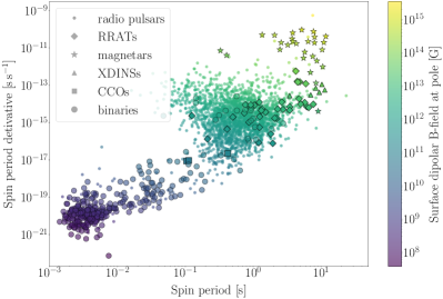
Figure 1: Period, $P$, vs period derivative, $\dot{P}$, plane for known pulsars. The bulk of the NS population is composed of radio pulsars given as dots. We also show Rotating Radio Transients (RRATs) as diamonds, highly magnetized magnetars as stars, X-ray Dim Isolated Neutron Stars (XDINSs) as triangles, Central Compact Objects (CCOs) as squares and spin-down driven NSs in binaries as circles. Note, however, that this figure does not include accreting X-ray binaries. Colors as indicated by the color bar on the right reflect the magnetic-field strength at the stellar pole inferred from $P$ and $\dot{P}$ measurements under the assumption of a dipolar configuration (see Sec. 3.6.1 for details). Data are taken from the ATNF catalogue [27, 28], the RRAT catalogue [18], the McGill Online Magnetar Catalogue [29, 30] and the Magnetar Outburst Online Catalog [31, 32].

Central Compact Objects: CCOs consist of radio quiet, thermally emitting X-ray sources with $k_{\rm B}T_{\rm BB}\sim 0.2-0.5\,$keV, which were discovered due to their locations at the centers of luminous shell-like supernova remnants (see [33, 34] for reviews). This association implies ages of at most a few tens of kyrs. Three CCOs show X-ray pulsations with periods in the $0.1-0.4\,$s range (see squares in Fig. 1), but have very low spin-down rates despite their young ages. The corresponding rotational energy reservoirs are insufficient to produce the observed X-ray emission. Their low inferred dipolar magnetic fields between $\sim 10^{10}-10^{11}\,$G, and the presence of thermally emitting hotspots are difficult to explain at the same time. This could be reconciled by strong magnetic fields buried in the interiors of CCOs following a phase of strong fallback accretion after the supernova [35]. This is supported by the fact that the characteristic ages, $\tau_{\rm c}$, of the three pulsed CCOs are orders of magnitude larger than the ages obtained from the SuNR association. However, the exact nature of these sources remains uncertain.

Accreting X-ray binaries: NSs in binary systems undergoing matter accretion from the companion star’s wind or via an accretion disk have been well known since the 1970s [e.g., 36]. These are mostly observed as bright X-ray sources with luminosities typically proportional to the mass accretion rate. For a general review see [37]. In particular, we know of accreting NSs with high-mass companions (aka high-mass X-ray binaries; around 300 objects known to date [38]) and those with low-mass companions (aka low-mass X-ray binaries; around 350 known to date [39]). Specifically, HMXBs are young systems ($\sim 0.1-10\,$Myr) characterized by NS magnetic fields of $\sim 10^{12}-10^{13}$ G, mostly accreting via wind and in wide, eccentric orbits. Their spin periods range between a few to thousands of seconds. On the other hand, LMXBs are older systems ($\sim 0.1-1\,$Gyr) with a fast spinning NS (about $1-100\,$ms), low magnetic fields of $\sim 10^{8}-10^{10}\,$G and tight orbits that typically accrete via Roche-lobe overflow and form large accretion disks. After this accretion phase which leads to a significant NS spin-up, binary pulsars often restart their rotation-powered emission with a short (recycled) spin period (see bottom-left objects depicted as circles in Fig. 1).

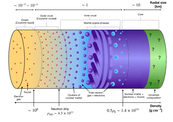
Figure 2: Artistic representation of the internal structure of a NS. We highlight the different NS layers as a function of the radial size (top axis) and density (bottom axis). The variation of color from red to purple in the crustal nuclei/nuclear-matter clusters represents an increase of neutron richness.

2.2 Neutron-star structure

In this section, we provide a brief overview of the current understanding of the internal NS structure and composition, which are summarized in the sketch in Fig. 2.

Starting from the outside, the outermost NS layer is the gaseous atmosphere (not represented in Fig. 2) with a thickness of $\mathcal{O}(10\,\textrm{cm})$, which encloses the ocean or envelope. Depending on the temperature, this ocean has a characteristic depth of $\mathcal{O}(1-100\,\textrm{m})$ [40] and is composed either of heavy elements (e.g., iron) or light elements (provided by accretion) in a Coulomb liquid state. If the magnetic field is strong and the temperature sufficiently low, a solid skin can form on top of the liquid phase (see, e.g., Fig. 10 of [40]).

Below the ocean lies a solid crust with a total thickness of $\mathcal{O}(1\,\textrm{km})$. The crust is divided into an outer crust and an inner crust. In the former, the atoms are fully ionized due to the intense pressure. The electrons form a degenerate relativistic gas, while the nuclei are organized in a Coulomb lattice. With increasing density, the nuclei become more and more neutron-rich due to electron captures. At the neutron-drip density, $\rho_{\rm ND}\approx 4.3\times 10^{11}\,\textrm{g}\,{\rm cm}^{-3}$, neutrons start dripping out from the nuclei, marking the transition to the inner crust. Here, the nuclei are so neutron-rich that they are more appropriately referred to as ‘clusters’ of nuclear matter. These spherical clusters form a lattice immersed in the gas of dripped neutrons. If the temperature is low enough, this neutron gas can experience a phase transition to a superfluid state (see Sec. 3.8). Moving deeper into the star, the density increases and the clusters grow and move closer to each other. Eventually, at the bottom of the inner crust, clusters cannot retain their spherical shape and merge into cylindrical structures of nuclear matter known as spaghetti. At even higher densities, the spaghetti merge into slab-like structures called lasagne. Moving deeper, lasagne merges, forming a matrix of nuclear matter confining the neutron gas, first in hollow cylinders and then into bubble-like structures. Although the presence of this so-called nuclear pasta has a negligible influence on the structure of the star, its anisotropic matter organization has a big impact on the NS transport properties (see Secs. 3.7.1 and 3.7.2). The region at the base of the inner crust characterized by the presence of nuclear pasta is sometimes also referred to as the mantle.

At densities of around $0.5\rho_{0}$, we transition from the inner crust to a state of pure nuclear matter, which marks the beginning of the NS core. The core has a radial size of around $10\,$km and contains the majority of the NS mass. This strongly degenerate liquid phase is composed primarily of neutrons with a small fraction of protons and electrons (and at higher densities also muons) to ensure charge neutrality. For NSs that are sufficiently cold, these core neutrons and protons may also undergo a superfluid and a superconducting transition, respectively (see Sec. 3.8). While densities at the center of NSs could reach up to $10^{15}\,{\rm g}\,{\rm cm}^{-3}$, our understanding of many-body physics becomes more uncertain at densities above $\rho_{0}$ and the NS composition, thus, unclear. However, at such extreme densities, the inner core of NSs could contain new particle species such as hyperons or even transition to more exotic states of matter like a Bose-Einstein condensate of pions and/or kaons or a quark-gluon plasma.

Assuming spherical symmetry, the mechanical structure of a NS is described by the Tolman-Oppenheimer-Volkoff equation [41, 42], which derives from the Einstein field equations of general relativity (GR) and the continuity of the stress-energy tensor. To solve this equation, we require knowledge of the functional relation between the pressure and the density, i.e. $P(\rho)$, a relation known as the EOS. An EOS generally relates three thermodynamic quantities, such as pressure, density, and temperature. In most applications concerning NSs, the temperature dependence can be neglected because it is much lower than its degeneracy limit. Such an EOS is known as barotropic. Roughly speaking, the EOS describes how matter reacts under compression: Stiff EOSs reflect those cases where an increase in density results in a significant increase in pressure, while soft EOSs refer to the opposite case. The NS EOS depends both on the nuclear interactions at extremely high densities, but also on the matter composition. At present the EOS of the outer crust is well established, while that of the inner crust and, in particular, the core EOS are much more uncertain, as we cannot test matter under such extreme conditions on Earth.

However, the dense-matter EOS, and in particular the EOS in the core, influences macroscopic properties of NSs, such as the star’s mass, radius, moment of inertia and tidal deformability. By measuring these quantities, it is, hence, possible to constrain the EOS. For example, the EOS determines the maximum mass a NS can attain, with stiff EOSs allowing for higher maximum masses. This way, measuring large NS masses allows us to rule out the softest EOSs. Similarly, each EOS leads to a unique relation between the mass and the stellar radius [43], or its moment of inertia [44]. As an example, mass-radius relations for a range of potential nuclear EOSs are illustrated in Fig. 3. Thus, measuring two of these quantities for one or more objects allows additional EOS constraints. Moreover, additional NS observables are sensitive to specific internal physics, which can help us further probe the properties of dense nuclear matter, such as superfluid physics. This way, NSs can serve as cosmic laboratories to test interaction and characteristics of matter at conditions that are not reproducible on the Earth. In the following, we discuss how such measurements are achieved.

We refer those readers interested in learning more about the structure and composition of NSs to [45] for a detailed review on the composition of the crust, to [40] for a review of NS transport properties, and [46, 47] for reviews on the NS structure and the dense-matter EOS.

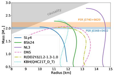
Figure 3: Mass-radius curves for a broad range of dense-matter EOSs. The solid lines show three nuclear EOSs: SLy4 [48, 49, 50] (blue), BSk24 [51, 52, 53, 54, 55] (green), and NL3 [56, 57, 58] (purple). The dashed line represents DNS [59, 60, 61] (pink), containing hyperons. The dashed-dotted line shows the EOS R(DD2Y$\Delta$) [62, 63, 64] (light green), which includes hyperons and $\Delta$ resonances, while the dotted line represents KBH(QHC21T$\_$D$\_$T) [65, 66] (light blue), characterizing NSs with quark matter cores. Measurements for two heavy radio pulsars, PSR J0740+662 [67] (orange) and PSR J0348+042 [68] (blue), are highlighted as horizontal bands. We also show the lower limit causality places on the NS radius as a gray shaded region in the top-left corner. EOS data are taken from the CompOSE database [69].

3 Neutron-star measurements

We now turn to discussing the various methods employed to extract different NS parameters. Each subsection is dedicated to one stellar property and details the different techniques to measure it. We summarize these techniques in a table at the beginning of each subsection and use three colors to represent the method’s degree of model dependency. Green identifies those approaches that are (relatively) model-independent, giving the most robust measurement of NS parameters. We use yellow to indicate methods that are somewhat model dependent and/or where the measurement of a quantity is correlated with other parameters, introducing significant uncertainty in the measured value. Finally, we use orange to classify those methods that are strongly model dependent. These methods typically rely on a range of assumptions that are either qualitative or not always fully justifiable, but nonetheless useful in modeling NS behavior. However, corresponding results and conclusions must be taken with caution.

We highlight that our color classification of the various methods is not fully rigorous but retains an inevitable degree of subjectiveness. However, we do provide justifications for our choice in all cases to help the reader understand our assessments.

3.1 Mass

Method		GWs	Radio	Optical	X-ray	$\mathbf{\gamma}$-ray
Binary mass function	1st MF
	+ 2nd MF
	+ 2nd MF + optical modeling
	+ 2nd MF + eclipses
	+ 1 PK parameter
	+ 2 PK parameters
Shapiro delay
GW in compact binary mergers
GW asteroseismology
Cooling
Lensing in eclipsing binaries

Table 1: Mass measurements. Individual rows represent the methods that provide NS masses, while columns denote different messengers/ EM wavebands. Colored cells represent the messengers/wavelengths at which the methods operate. Green characterizes those techniques that are (almost) model independent, yellow those that are somewhat model dependent and/or affected by degeneracy, and orange those methods that are strongly model dependent. Note that we split the binary-mass-function approach into different subversions, where MF = mass function and PK = post-Keplerian. All techniques are discussed in detail in the text.

The first parameter of interest is the NS mass, $M_{\rm NS}$. The mass is particularly important because its maximum value is closely connected to the EOS of dense matter, i.e., large masses exclude those EOSs that are not sufficiently stiff to account for that measurement. Fig. 3 shows the mass-radius plane and mass constraints for two radio pulsars. Moreover, combining a measured mass with a radius or moment-of-inertia measurement allows us to pin down specific EOSs.

As we discuss below, NSs in binary systems constitute the best targets to provide precise and model-independent measures for this quantity, while observables from isolated compact objects generally provide more model-dependent mass estimates.

3.1.1 Binary mass function

For NSs in binary systems, we can exploit Newtonian dynamics to constrain their masses. Using Kepler’s third law, we can define the binary mass function as [e.g., 70]:

$$f_{\rm bin}(M_{\rm c},M_{\rm NS})\equiv\frac{M^{3}_{\rm NS}\sin^{3}i}{(M_{\rm c}+M_{\rm NS})^{2}}=\frac{K^{3}_{\rm c}P_{\rm orb}}{2\pi G}(1-e^{2})^{3/2},$$ (1)

where $M_{\rm c}$ and $M_{\rm NS}$ are the mass of the binary companion and the NS, respectively, $i$ is the angle between the line of sight (LOS) and the system’s orbital angular momentum (i.e., the inclination angle), $K_{\rm c}$ is the radial velocity of the companion, $P_{\rm orb}$ and $e$ are the period and the eccentricity of the orbit, respectively, and $G$ denotes the gravitational constant. It is worth noting that the right-hand side of Eq. (1) contains observable quantities, which can be measured by radio timing if the companion is a radio pulsar or by optical spectroscopy if the companion is a non-compact star or a white dwarf (WD). Measuring $f_{\rm bin}$, thus, allows us to constrain $M_{\rm NS}$ (specifically obtain a lower limit) but not to determine it explicitly because of the degeneracy with $M_{\rm c}$ and the binary inclination, $i$.

The degeneracy with respect to $M_{\rm c}$ can be broken if the NS’s radial velocity, $K_{\rm NS}$, (or equivalently the projection of the semi-major axis of the NS’s orbit onto the observer plane) is also measured. This allows for the determination of an additional mass function, $f_{\mathrm{bin}}(M_{\mathrm{NS}},M_{\mathrm{c}})$, (namely Eq. (1) after exchanging the $\mathrm{NS}$ and $\mathrm{c}$ subscripts, referred to as the 2nd mass function in Tab. 1). The ratio of these two mass functions allows us to obtain the mass ratio, $M_{\rm c}/M_{\rm NS}$, which is equal to $K_{\rm NS}/K_{\rm c}$ following Eq. (1), and represents a further constraint for our system. We classify both these mass-function approaches as yellow in Tab. 1.

The degeneracy with respect to the inclination angle can be resolved by measuring the so-called Shapiro delay (see Sec. 3.1.2), modeling of the optical lightcurve in case of a non-degenerate companion [71, 72, 73, 74, 75, 76] or by the observation of eclipses [77, 78, 79, 80, 81, 82]. Prime targets for the latter two kinds of studies are so-called ‘spiders’, millisecond pulsars (i.e., those NSs with millisecond periods, which are located in the bottom left of the $P-\dot{P}$ plane in Fig. 1) in compact binaries with $P_{\mathrm{orb}}\lesssim 1\,\mathrm{day}$ and orbital separation $a\sim R_{\odot}$, whose relativistic winds are strong enough to heat and ablate matter from their companion [83, 84, 85, 86, 87]. Those systems with a companion mass $M_{\rm c}=\mathcal{O}(0.01\,M_{\odot})$ are called black widows [e.g., 84], while those with a companion mass $M_{\rm c}=\mathcal{O}(0.1\,M_{\odot})$ are referred to as redbacks [e.g., 85] (see also [87] for a systematic study of redbacks).

Optical lightcurve modeling exploits the fact that in a sufficiently compact binary, the companion star will be tidally deformed and heated on one side by the irradiation from the NS. Both effects impact the optical lightcurve in an inclination-dependent way. Consequently, accurate modeling of the lightcurve allows us to break the degeneracy with $\sin i$. However, the problem with this method resides in its strong model dependency, which may introduce systematic biases due to the incompleteness of heating models [88, 89, 82]. For this reason, we classify the determination of the inclination through optical modeling as orange in Tab. 1.

Nonetheless, spiders are particularly interesting targets for this kind of measurement as the NS companion is often optically bright. This brightness allows for the determination of the companion’s radial velocity via optical spectroscopy, while the NS’s radial velocity can be obtained through pulsar timing. However, care has to be taken when measuring the companion velocity, since irradiation from the NS heats one side of the star, shifting the center of light away from the companion’s center of mass towards the binary’s center of mass. If not corrected for, this effect causes the measured velocity to underestimate the true value, leading to an underestimation of the pulsar mass (see Eq. (1) and [82]).

In contrast, the eclipse of the NS emission by its companion or vice versa points towards a system observed with an edge-on orientation, such that $\sin i\sim 1$, providing a less model-dependent inclination constraint. The eclipse signal is typically searched for in the X-ray and gamma-ray bands, because those energies are less affected by absorption and scattering from the inter-binary diffuse material. We, however, note that X-ray eclipses in spiders can be masked by the X-ray emission from inter-binary shocks [90], which are generated by encounters of the pulsar wind and that of the companion [82]. Thus, spider systems are primarily targeted in the gamma-rays. Studying 42 spiders (plus seven redback candidates), [82] for example recently identified five eclipsing systems (plus two among the candidates) and excluded the presence of gamma-ray eclipse in 32 of them. These observations led to constraints on the NS masses in eclipsing binaries and the identification of lower NS mass limits in non-eclipsing systems, an approach which we classify as yellow in Tab. 1.

We also note that such measurements hint at the fact that spiders are higher in mass than other NSs in binary systems [91, 92], consequently allowing for interesting constraints on the EOS-dependent NS maximum mass. For example, the highest masses in eclipsing systems found by [82] are associated with the black widow B1957+20 [84], with $M_{\mathrm{NS}}=1.67-1.94\,M_{\odot}$, and the redback J1816+4510, with $M_{\mathrm{NS}}=1.64-2.17\,M_{\odot}$ [93]. The former mass estimate is lower than what was previously inferred from optical modeling for B1957+20 (i.e., $M_{\mathrm{NS}}=2.4\pm 0.1\,M_{\odot}$ [94]), highlighting the importance of complementary mass measurements and the quantification of underlying systematics.

Other means to break the mass-function degeneracy is by measuring two or more post-Keplerian parameters (that capture deviations from Keplerian motion as expected in the theory of GR) through radio pulsar timing. According to GR, post-Keplerian parameters depend on the system’s mass and inclination. MSP are particularly promising for measuring post-Keplerian effects, as their rotational stability provides highly stable pulsar timing solutions. Besides Shapiro delay, which we dedicate the next section to, other useful post-Keplerian parameters are the periastron advance, $\dot{\omega}$ (which is typically the easiest to measure [12]), the rate of orbital decay due to GW emission, $\dot{P}_{\rm orb}$, and the Einstein delay, $\gamma$, due to time dilation and the gravitational redshift. These are defined as [e.g., 70]:

$$\dot{\omega} =3\left(\frac{P_{\rm orb}}{2\pi}\right)^{-5/3}\left(1-e^{2}\right)^{-1}\left(T_{\odot}M\right)^{2/3},$$ (2)

$$\dot{P}_{\rm orb} =-\frac{192\pi}{5}\left(\frac{P_{\rm orb}}{2\pi}\right)^{-5/3}d(e)\,T^{5/3}_{\odot}\frac{M_{\rm c}M_{\rm NS}}{M^{1/3}},$$ (3)

$$\gamma =\left(\frac{P_{\rm orb}}{2\pi}\right)^{1/3}eT^{2/3}_{\odot}\frac{M_{\rm c}(M_{\rm NS}+2M_{\rm c})}{M^{4/3}},$$ (4)

where $M\equiv M_{\rm c}+M_{\rm NS}$ is the total mass of the system, measured in units of $M_{\odot}$. Moreover, $T_{\odot}\equiv GM_{\odot}/c^{3}=4.92549\,\mu$s (where $c$ denotes the speed of light), and $d(e)\equiv(1+73e^{2}/24+37e^{4}/96)(1-e^{2})^{-7/2}$.

The above formulae depend on GR only, a theory whose predictions have been validated to subpercent level in several double NS systems that contain pulsars [e.g., 95, 96, 97]. Consequently, measuring the mass function plus two (or more) of these post-Keplerian parameters provides a relatively model-independent way to measure the mass of a NS (see classification in Tab. 1).

We conclude by stressing that the relative uncertainty of these post-Keplerian parameters decreases with increasing observing time [98]. On the contrary, a larger orbital period tends to increase the fractional uncertainties of most Keplerian parameters. For the exact scalings of various fractional uncertainties with the observation time span and the orbital period, we refer the interested reader to Tab. 2 of [98] or Tab. 8.2 of [12].

3.1.2 Shapiro delay

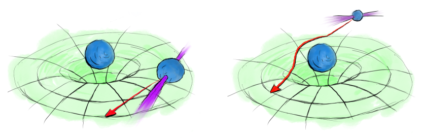
Figure 4: Artistic representation of the Shapiro delay in a binary NS system. While the signal from a pulsar is primarily unaltered by its NS companion in inferior conjunction (left), the signal is affected by the companion’s curvature introducing a time delay when the pulsar is in superior conjunction (right).

Besides the above post-Keplerian parameters, Shapiro delay provides a straightforward and precise way to measure NS masses in a model-independent manner. Shapiro delay is a gravitational effect predicted by GR that occurs when a signal-carrying messenger (e.g., a photon) passes near a massive object. As the messenger traverses the curved spacetime around the object, its trajectory is altered, resulting in an increased time of flight and subsequent delay in the arrival of the signal [99]. This delay is influenced by the value of $\sin i$ and the spacetime curvature, which in turn is determined primarily by the object’s mass. A graphical representation of this effect is illustrated in Fig. 4.

Measurement of the Shapiro delay is particular effective to determine the masses of NSs in BNS systems, where at least one of the NSs is a radio pulsar, whose radio beam passes closely by its companion during a specific orbital phase. By precisely measuring the arrival times of the radio pulses, the Shapiro delay can be accurately determined, enabling the estimation of the mass of the pulsar’s companion [100, 101]. Nevertheless, the effect can also be used to determine the masses of pulsars and their companions in other kind of systems, such as those with a WD companion [102, 103, 104, 105, 106, 107] (see Eqs. (5) and (6) for details).

From an observational point of view, once a model for the arrival times of the radio pulses (in absence of Shapiro delay) is defined, the Shapiro delay appears as a characteristic cusp in the residuals at superior conjunction. At this point, the pulsar is located behind its companion relative to the observer and the signal, thus, traverses the largest amount of spacetime curvature. The timing model accounting for this effect can then be modeled by two parameters, $r$ and $s$, called the Shapiro delay range and shape, respectively. These are functions of the companion mass, $M_{\rm c}$, and the system’s inclination angle, $i$, respectively, [108, 109, 12]:

$$r \equiv T_{\odot}M_{\rm c},$$ (5)

$$s \equiv\sin i$$

$$=T^{-1/3}_{\odot}\left(\frac{P_{\rm orb}}{2\pi}\right)^{-2/3}x\,\frac{\left(M_{\rm c}+M_{\rm NS}\right)^{2/3}}{M_{\rm c}},$$ (6)

where $M_{\rm c,NS}$ are measured in solar masses and the second equality in Eq. (6) was obtained from Eq. (1) after substituting $K_{\rm NS}=a_{1}\sin i(2\pi/P_{\rm orb})(1-e^{2})^{-1/2}$. Here, $a_{1}$ is the orbit’s semi-major axis, and we define the projected semi-major axis as $x\equiv a_{1}\sin i/c$. We, however, note that the parametrization of the timing solution in terms of $r$ and $s$ is not unique [e.g., 110].

Due to the possibility of timing radio pulsars, and the simplicity of the effect which ultimately depends only on GR, Shapiro delay presents a precise and model-independent way to constrain the mass of a NS. It is easiest to detect in binaries that contain heavy companions, because $M_{\rm c}$ directly affects the amplitude of the Shapiro delay, and MSPs, which can be observed with microsecond-level timing precision or better. Consequently, this approach has played a pivotal role in detecting several NSs with masses above $2\,M_{\odot}$ [111, 100, 112], leading to groundbreaking results in the field and the tightest constraints on the dense-matter EOS. We stress, though, that this effect is observable primarily in systems that have a favorable orientation with respect to the observer, namely those that are close to edge-on ($\sin i\sim 1$).

3.1.3 Gravitational waves from compact binary mergers

Binary systems lose their orbital energy due to the emission of GWs. If a system is sufficiently massive and compact, this energy loss causes an observable shrinking of the orbit, eventually leading to the objects’ merger. This can occur in binaries formed by two compact objects, such as NSs.

Such a compact binary merger (CBM) can be formally divided into three different phases: an inspiral, a merger, and a ringdown phase. In particular, the inspiral is the phase in which the two objects are not yet in contact, and, with the exception of the final orbits, can be treated as point masses as their finite sizes play a negligible role in the dynamics. In this phase, the system’s evolution is simple: the system emits GWs at a frequency, $f_{\rm GW}$, that is twice the Keplerian orbital frequency, and with an amplitude proportional to $f^{2/3}_{\rm GW}$. The orbital shrinking results in an increase of the Keplerian frequency, consequently increasing the GW frequency and amplitude. The resulting waveform has a characteristic shape and is called chirp signal. During this phase, the frequency evolution is described by the following equation [113]:

$$\dot{f}_{\rm GW}=\frac{96}{5}\pi^{8/3}\left(\frac{G\mathcal{M}}{c^{3}}\right)^{5/3}f^{11/3}_{\rm GW},$$ (7)

where

$$\mathcal{M}\equiv\frac{(M_{\rm c}M_{\rm NS})^{3/5}}{(M_{\rm c}+M_{\rm NS})^{1/5}}$$ (8)

is a combination of the masses $M_{\rm NS,c}$ known as the chirp mass. Since both $\dot{f}_{\rm GW}$ and $f_{\rm GW}$ are measurable through the observation of GWs from a CBM, Eq. (7) can be used to determine the chirp mass of the system. Although measuring $\mathcal{M}$ does not allow us to deduce the mass of the NS itself, it provides an important constraint in the $M_{\rm c}-M_{\rm NS}$ plane.

As we approach the merger, the GW signal becomes more and more sensitive to relativistic effects, which depend on the binaries’ mass ratio [114, 115]. Hence, comparing a signal of sufficiently high signal-to-noise ratio (SNR) with predicted GW waveforms can be employed to put tighter constraints on the NS mass [1]. We stress, however, that similar effects can also be mimicked by other processes related to the spins of both objects. This leads to a degeneracy between the effective spin (a weighted combination of the objects’ spins and masses) and the mass ratio [114, 115]. As a result, we classify this method as yellow in Tab. 1.

3.1.4 Gravitational-wave asteroseismology

When perturbed from its equilibrium configuration, a NS (approximated as a fluid) is subjected to several damped oscillatory modes, known as quasi-normal modes. If these perturbations are non-radial and drive variations in the star’s quadrupole moment, quasi-normal modes are associated with the emission of GWs [116, 113]. A detection of GWs excited by such quasi-normal modes will allow us to constrain the stellar mass and radius, or any other quantity derived from both parameters, such as the compactness (see also Sec. 3.5) or the average density. This technique is known as the inverse problem in GW asteroseismology.

The central idea relies on the existence of several quasi-universal relations (namely, expressions that are only weakly dependent on the choice of EOS), which link the modes’ frequencies and their characteristic damping times to a given combination of the NS mass and radius [117, 118, 119] or other bulk quantities like the moment of inertia [120] or the tidal Love number [121] (for a definition of the Love number see Sec. 3.4). These quasi-universal relations hold in particular for the so-called $f$-mode and the $w$-modes, which depend primarily on macroscopic NS quantities.

The $f$-mode is the fluid’s fundamental mode. It is a non-radial mode that has no nodes inside the interior of the star. Its frequency lies in the range of $1.5-3\,\textrm{kHz}$, namely within the frequency window of terrestrial interferometers, while its damping time ranges between $0.1-0.5\,\textrm{s}$ [122]. The lack of nodes in the interior of the star makes the $f$-mode weakly dependent on the detailed microphysics of matter, but instead dependent on the global properties of the star. In particular, the mode frequency can be tightly connected to the average density $\bar{\rho}=M_{\rm NS}/R_{\rm NS}^{3}$ via:

$$\omega_{f}\simeq a_{f}+b_{f}\left(\frac{\bar{M}_{\rm NS}}{\bar{R}_{\rm NS}^{3}}\right)^{1/2},$$ (9)

where $\bar{M}_{\rm NS}$ and $\bar{R}_{\rm NS}$ are dimensionless parameters that normalize the mass and radius to $1.4\,M_{\odot}$ and $10\,\textrm{km}$, respectively, and $\omega_{f}$ is measured in kHz. [117] determined the values of the fitting parameters $a_{f}$ and $b_{f}$ to $0.78$ and $1.635$, respectively. We, however, highlight that the exact values of these coefficients (and those presented below) are somewhat dependent on the sample of realistic EOSs used to fit the quasi-universal relations.

We note that a similar fundamental relation also exists for the $f$-mode damping time, $\tau_{f}$, which can be expressed as a function of the stellar compactness (see Sec. 3.5) [117]:

$$\frac{\bar{R}^{4}_{\rm NS}}{\bar{M}^{3}_{\rm NS}}\frac{1}{\tau_{f}}\simeq c_{f}-d_{f}\left(\frac{\bar{M}_{\rm NS}}{\bar{R}_{\rm NS}}\right).$$ (10)

Here, $c_{f}=22.85$ and $d_{f}=14.65$ [117] and the damping $\tau_{f}$ is measured in seconds. A combined measurement of the mode frequency and its damping time, thus allows us to determine the stellar mass and the radius.

Another set of universal relations can be found for the $w$-modes. Instead of involving fluid motions, these are oscillations of spacetime itself [123]. As such, they are insensitive to the dense-matter EOS. Compared to the $f$-mode, $w$-modes are characterized by higher frequencies (around $5-12\,\textrm{kHz}$ for the lowest-order modes) and shorter damping times of the order of $\mathcal{O}(0.01\,\textrm{ms})$. Their universal relations are [117]:

$$\bar{R}_{\rm NS}\omega_{w} \simeq a_{w}-b_{w}\left(\frac{\bar{M}_{\rm NS}}{\bar{R}_{\rm NS}}\right),$$ (11)

$$\frac{\bar{M}_{\rm NS}}{\tau_{w}} \simeq c_{w}+d_{w}\left(\frac{\bar{M}_{\rm NS}}{\bar{R}_{\rm NS}}\right)-e_{w}\left(\frac{\bar{M}_{\rm NS}}{\bar{R}_{\rm NS}}\right)^{2},$$ (12)

where $a_{w}=20.92$, $b_{w}=9.14$, $c_{w}=5.74$, $d_{w}=103$ and $e_{w}=67.45$. Here, contrary to Eq. (10), the damping time $\tau_{w}$ is measured in milliseconds. Similar relations for the $f$-mode and the $w$-modes have been also found by several other authors [e.g., 118, 124, 119, 125, 126, 127, 128].

Additional modes of interest are the so-called $p$-modes or $g$-modes. $p$-modes, or pressure modes, are fluid modes where the gradient of the pressure acts as the restoring force. Their frequency is much more dependent on the EOS than for the modes previously discussed, and they are not expected to lead to tight universal relations [117]. These modes are, however, interesting because if the mass, the radius, or another combination of these quantities are known, a measurement of the $p$-mode frequency may allow us to constrain the EOS [117]. $g$-modes, or gravity modes, have buoyancy as the restoring force [129]. They are particularly sensitive to the NS composition and the presence of discontinuities between different phases of matter [130]. As such, $g$-mode frequency measurements may provide insights into the presence of hyperonic matter [e.g., 131] and the transition from hadronic to quark matter in the NS core [e.g., 132, 133].

The discussion so far concerns non-rotating NSs. Here, the frequency of a given mode is characterized by the spherical degree $l$ only, while there is a ($2l+1$)-degeneracy in the azimuthal order $m$, i.e., $m=-l,...,l$. Rotation has the effect of breaking this degeneracy, splitting a mode with degree $l$ into $2l+1$ modes with distinct frequencies [134, 135, 136]. This mode splitting is more pronounced for faster rotation, such that the mode frequency normalized to its value in the non-rotating limit can be expressed as a quadratic function of the rotational frequency [134, 135, 136]. Consequently, rotation introduces an additional parameter (the NS’s angular velocity) to the inverse problem in asteroseismology.

This method is generally affected by two main issues. First, albeit the universal relations presented above holding for a large sample of hadronic and hybrid EOSs, the latter characterizing those stars where quark-matter cores are surrounded by hadronic matter, they might not be satisfied by EOSs for stars with exotic compositions, such as bare quark stars that do not contain a hadronic shell [e.g., 119]. For this reason, we classify this method as yellow in Tab. 1.

The second problem concerns the detectability of NS quasi-normal modes. Estimating the mode energy required for detection with different GW facilities, [137] find that a measurement of the $f$-mode frequency with an uncertainty of $1\%$ using second-generation interferometers requires a mode energy of $\mathcal{O}(10^{-11}\,M_{\odot}c^{2})$ for a Galactic source at a distance of $10\,\textrm{kpc}$. The required energy increases considerably to $\mathcal{O}(10^{-4}\,M_{\odot}c^{2})$, if we also want to measure the damping time with the same precision. The situation is further complicated for $w$-modes, which are unlikely to be detected with present facilities [137]. Consequently, any detectable GWs associated with quasi-normal modes have to be excited by violent events, such as supernova explosions or magnetar giant flares (see Sec. 3.5.3). However, the rates of these events are low if we are confined to our Galaxy [e.g., 138, 139, 140], the most likely explanation for why we have not observed these signals yet. This situation should improve with the advanced sensitivity of next-generation facilities [141, 142], which will allow detection of such signals from nearby galaxies [143]. For example, third-generation GW detectors are expected to detect Galactic sources within $10\,\rm kpc$, if the mode energy is greater than $\mathcal{O}(10^{-12}\,M_{\odot}c^{2})$ and within the Andromeda galaxy for mode energies above $\mathcal{O}(10^{-8}\,M_{\odot}c^{2})$ [144], making future detections more likely.

3.1.5 Cooling

NSs emit thermal radiation in the X-rays. By tracking their temperature evolution, we indirectly gain information on the stellar mass. Specifically, during its life, a NS looses its thermal energy due to neutrino emission from its whole volume (which is transparent to neutrinos) and photon emission from its surface [145, 146, 147, 148, 40] (see Fig. 5).

Neutrino cooling, which dominates during the first $10-100\,\mathrm{kyr}$ of a NS’s life, is composed of different emission mechanisms, whose relevance depends on the stellar mass. In particular, one of the most efficient neutrino cooling processes is the direct Urca process [149], which consists of the following electron-capture and $\beta$-decay reactions:

$$p+e^{-}\rightarrow n+\nu_{\rm e},$$ (13)

$$n\rightarrow p+e^{-}+\bar{\nu}_{\rm e},$$ (14)

where the neutrino and the antineutrino escape from the star and act like an energy sink. The process strongly depends on the temperature, with a neutrino emissivity $\propto T^{6}$ (see, e.g., Eq. (120) of [150]), and may occur in the NS core provided that the proton fraction is sufficiently high [151, 152]. Since the proton fraction increases with increasing central pressure, and the central pressure increases with increasing mass, the presence of direct Urca ultimately depends on the stellar mass. Rapid cooling of young compact objects could, therefore, be an indication for heavy NSs.

In absence of direct Urca reactions, the main contributor to NS cooling is the so-called modified Urca process, which substitutes the $\beta$-decay reaction (14) as follows:

$$n+n\rightarrow n+p+e^{-}+\bar{\nu}_{\rm e}.$$ (15)

This process has a steeper temperature dependence, with a neutrino emissivity scaling as $T^{8}$. This results in a shallower decrease of the temperature, $T$, with time, $t$, which scales as $T(t)\propto t^{-1/6}$. In contrast, direct Urca leads to $T(t)\propto t^{-1/4}$. In both cases, we are assuming an isothermal star with a heat capacity $C_{v}\propto T$ (see [150] for a review).

As an example, Fig. 5 shows a comparison between the cooling curves of two NS models characterized by the same EOS, but two different masses. The heavier object (orange curve) is able to activate direct Urca processes causing the core to cool very fast in the first years. This results in a steep drop of almost four orders of magnitude in luminosity within the first $50\,\mathrm{yr}$. Direct Urca cooling then proceeds until at around $10^{5}\,\mathrm{yr}$ when the emission of photons from the surface becomes the dominant mechanism and the cooling curve steepens again. Instead, the low-mass case (blue curve) is controlled by slower modified Urca cooling and the luminosity does not suffer a sharp initial drop. Note, however, that both processes suffer strong quenching if neutrons are in a superfluid state (see Sec. 3.8.2) [150].

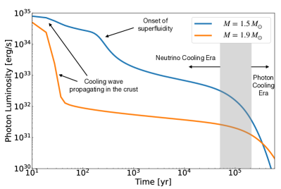
Figure 5: Comparison between two cooling curves for two NSs of different masses for the EOS BSk24 [51, 52]. The heavier object of $1.9\,M_{\odot}$ (orange) initially cools faster than the lighter $1.5\,M_{\odot}$ NS (blue) due to the fast cooling provided by direct Urca processes. We also label several additional physical processes. In particular, the gray shaded region represents the (approximate) time interval during which NS cooling transitions from neutrino-dominated to photon-dominated.

While efficient NS cooling due to direct Urca constrains stellar masses, we must take into account several difficulties, from the theoretical and observation sides. We first point out that the mass threshold for the activation of the direct Urca process depends on the stellar composition [70]. For example, the presence of hyperons or strange-quark matter affects NS cooling because similar, direct Urca-like processes involving these particle species could take place [153, 154, 155, 147]. Moreover, other efficient neutrino-emission processes contribute to NS cooling, such as neutrino emission due to the continuous breaking and formation of Cooper pairs (see Sec. 3.8.2) [150]. Finally, if NSs are strongly magnetized (as is the case for magnetars), we also have to account for additional heating due to the dissipation of electric currents. This in turn depends on the resistivity of the NS interior and the unknown magnetic-field geometry [156, 157, 158, 159].

From the observational side, we note that an accurate and precise determination of the NS cooling history requires reliable age estimates. While for those sources, embedded in their SNRs, this is typically possible by tracing back the remnant’s expansion history, ages are less certain for those NSs without remnants. In particular, rough estimates are obtained by identifying the NS’s true age with the characteristic age, $\tau_{\rm c}$ (see Sec. 2.1). This age measure is, however, not reliable because it does not take into account additional physics such as magnetic-field decay or fallback accretion [160, 161, 162] that can impact the spin-down history of the star. Uncertain age estimates, hence, significantly hamper a reliable determination of thermal evolution. Contrasting cooling models with data is further complicated by uncertainties in distance estimates, which are reflected in luminosity uncertainties.

In conclusion, while NS cooling is fundamental to constraining phenomena occurring in the star’s interior, and can provide hints on the stellar mass, it does provide neither a precise nor an accurate, or a model-independent channel to measure the NS mass. We hence classify this method as orange in Tab. 1.

3.1.6 Gravitational microlensing

Compact matter distributions act as gravitational lenses and bend the light of a bright source in the background, producing distorted and magnified images of this background source [163, 164, 165]. So-called gravitational microlensing is sensitive to Galactic stellar and compact-object lenses, such as NSs [164, 166, 167, 165]. While gravitational microlensing can, in principle, be used to measure the masses of isolated NSs that lens stars in their backgrounds [168, 169, 170, 171] such signals are weak and ridden with systematics [172, 170, 173], and NS in binaries, hence, more promising targets.

Here, gravitational lensing can take place, if the system is observed edge-on (i.e., $\sin i\sim 1$ and exhibiting eclipses) and the companion emits in the optical waveband. The resulting amplification of the companion’s optical lightcurve then depends on the lens mass, $M_{\rm NS}$, and the orbital separation, $a$. Specifically, the fractional amplification, defined as the ratio between the amplified flux and the companion’s unlensed flux, can be written as [174]:

$$f_{\rm amp}=2\left(\frac{R_{\rm e}}{R_{\rm c}}\right)^{2}=\frac{8GM_{\rm NS}}{c^{2}a}\,\left(\frac{a}{R_{\rm c}}\right)^{2},$$ (16)

where $R_{\rm e}$ is the Einstein ring’s radius and $R_{\rm c}$ the radius of the companion star. If the companion is filling its Roche lobe, the ratio $R_{\rm c}/a$ can also be expressed as a function of the system’s mass ratio [174].

Despite its apparent simplicity, the problem with this method is that in real systems the effect is expected to be small (of the order of $10^{-3}\,\mathrm{mag}$). As a result, it is typically overwhelmed by the intrinsic variability of the companion star, or by systematic uncertainties in the modeling of the optical lightcurve due to our incomplete understanding of the heating of the companion by the NS [174, 82] as already discussed earlier in Sec. 3.1.1.

As a result, microlensing is classified as strongly model dependent in Tab. 1. We also point out that we consider this approach the least promising of those discussed in Sec. 3.1 and primarily highlight it here for completeness.

3.2 Radius

Method	GWs	Radio	Optical	X-ray	$\mathbf{\gamma}$-ray
Surface emission spectral modeling
Photospheric radius expansion
X-ray lightcurve modeling
NS-BH merger + GRB
GW asteroseismology

Table 2: Radius measurements. Individual rows represent the methods that provide NS radii, while columns denote different messengers/EM wavebands. Individual colors are equivalent to those in Tab. 1. All techniques are discussed in detail in the text.

We next turn to those methods aimed at measuring the NS radius, $R_{\rm NS}$. As discussed in Sec. 2.2, a radius estimate coupled with a mass measurement for the same object would allow a constraint of the dense-matter EOS (see Fig. 3). However, despite its importance, the stellar radius is an elusive quantity and difficult to measure reliably. All techniques presented here (summarized in Tab. 2) are characterized by a certain degree of model dependence and/or lead to results that are degenerate with other parameters. Most of the approaches involve observations in the X-ray band, which are divided primarily into spectral and energy-resolved timing methods. We will discuss why the latter generally lead to more robust $R_{\rm NS}$ estimates. Finally, we report on those methods involving GW detections, which require detailed knowledge of the NS structure and the processes following compact-object mergers.

3.2.1 Spectral modeling of surface emission

For the NSs whose X-ray fluxes are dominated by thermal black-body emission from their surfaces, we can exploit the Stefan-Boltzmann law to measure $R_{\rm NS}$ [175, 70]. This method requires knowledge of surface temperatures, accessible through spectral analysis, along with reliable estimates of the source distances. It has been successfully applied to LMXBs in a quiescent state [176, 177, 178, 179, 180, 181, 182, 183, 184, 185, 186], during which we can reasonably assume that the contribution of accretion to the observed flux is absent or negligible, and CCOs [187, 188, 189, 190].

The Stefan-Boltzmann law allows us to write the source’s apparent radius, $R_{\infty}$, as

$$R_{\infty}=\sqrt{\frac{D^{2}F_{\infty}}{\sigma_{\rm SB}T^{4}_{\rm BB}}},$$ (17)

where $D$ denotes the distance, $F_{\infty}$ the bolometric flux, $\sigma_{\rm SB}$ the Stefan-Boltzmann constant and $T_{\rm BB}$ the black-body temperature of the star. Due to the NS’s compactness, this apparent radius differs from the true radius as a result of light bending in the curved spacetime around the compact object:

$$R_{\infty}=\left(1-2C_{\rm NS}\right)^{-1/2}R_{\rm NS},$$ (18)

where $C_{\rm NS}$ is the NS compactness (see Sec. 3.5 for details) defined as follows:

$$C_{\rm NS}\equiv\frac{GM_{\rm NS}}{c^{2}R_{\rm NS}}.$$ (19)

Equating relations (17) and (18), thus, allows us to deduce $R_{\rm NS}$. To date, this method has been used for $\mathcal{O}(10)$ LMXBs in globular clusters [178, 179, 180, 182, 191] and a comparable number of sources in the Galactic disk [183], leading to a wide range of radius estimates between $10-14\,\rm km$ (see, e.g., Fig. 4 of [175]). Note, however, that the appearance of the NS compactness in Eq. (18) (see Sec. 3.5 for details) introduces an additional dependence on the NS mass [192, 193]. This causes a degeneracy in the radius measurement, which would be absent in a non-relativistic picture.

Although simple in concept, this technique is based on several simplifications. First, it assumes that the NS surface has a uniform temperature, $T_{\rm BB}$. This is in general not true, especially for magnetars where the thermal conductivity is anisotropic due to the presence of strong magnetic fields (see, e.g., [40] for a review), and currents in the magnetosphere can heat the stellar surface at the footprints of the current-carrying magnetic-field bundle [194, 195, 196]. As a result, NSs are characterized by complex surface temperature distributions. Corresponding ‘hot spots’ are typically observed as periodic modulations in the X-ray flux at the stellar rotation frequency due to the spots’ regular occultation. However, the absence of such a pulsed flux is no guarantee for a uniform temperature, because similar behavior is also possible for systems with favorable geometry (e.g., a quasi-axisymmetric temperature map aligned with the rotation axis, or a rotation axis that is aligned with the LOS; see, e.g., Fig. 8 of [197]) or highly multipolar temperature maps, where the individual contributions of hot spots are smeared out [198]. In general, the presence of undetected hot spots leads to an underestimation of the stellar radius [199].

Another assumption concerns the fact that flux contributions from the stellar magnetosphere or the accretion disk are generally negligible. Moreover, the lack of knowledge of the NS’s atmospheric composition can be a further source of systematic error. For example, considering an atmosphere dominated by helium rather than hydrogen results in systematically larger inferred radii [200, 201]. Additionally, in the case of fast spinning NSs, relativistic corrections should also include the contribution from gravitomagnetic effects, which introduce dependencies on the spin, the mass and the inclination angle. For example, [202] report that for a star with $R_{\rm NS}=10\,\rm km$ rotating at $600\,\rm Hz$, the correction is of the order of $\sim 1-4\%$ (with higher values referring to higher inclinations, i.e., an edge-on view), while it rises to $2-12\%$ for a star with $R_{\rm NS}=15\,\rm km$. Finally, additional uncertainties may arise from difficulties in reliably measuring the distance of the source, which can be overcome by selecting sources in globular clusters, or modeling the interstellar extinction [203, 179].

All these caveats discussed here lead us to classify this method as strongly model dependent (orange) in Tab. 2.

3.2.2 Photospheric radius expansion

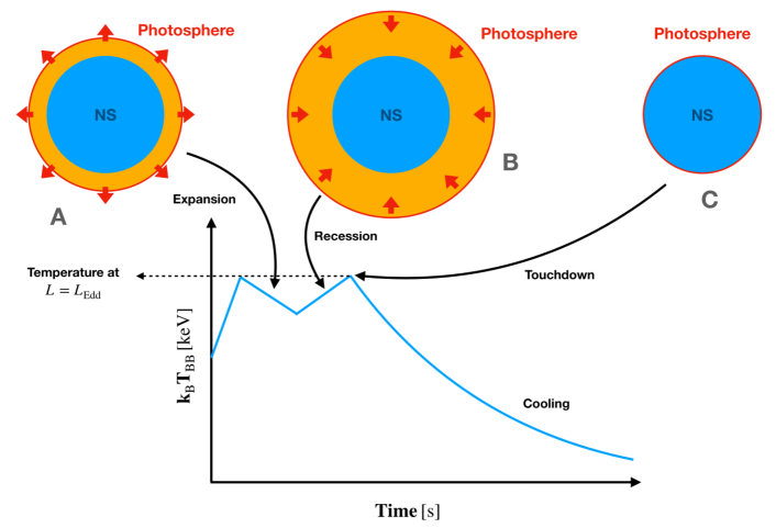
Figure 6: Illustration of the photospheric-radius-expansion scenario and the evolution of the NS’s thermal energy with time: During a thermonuclear X-ray burst a star is heated up significantly. As a result the stellar photosphere is lifted and the temperature decreases (A). After reaching a maximum expansion, the photosphere recedes (B), causing the temperature to increase. At the final touchdown phase (C), the photosphere reaches the stellar surface (providing a measure of $R_{\rm NS}$) and the temperature is maximal. At this stage, the star has a luminosity that takes the Eddington value. Subsequently, the NS resumes cooling without interruption. The units on the axes reflect fiducial orders of magnitude for the process, with typical temperatures of a few $\mathrm{keV}$ and durations of a few tens of seconds.

Other intriguing targets for measuring NS radii through spectral analysis are systems that undergo thermonuclear (Type-I) X-ray bursts [204, 205, 206, 207, 208, 209, 210, 211]. These phenomena occur when material, accreted from a companion star, accumulates on the stellar surface until a runaway fusion reaction is ignited (see Sec. 3.7.2 for more details).

The spectra of these X-ray bursts can be fitted with a black body, and in several cases, the temporal evolution of the temperature shows a peculiar two-peaked shape. This is characterized by an initial rise, a first decrease, a second rise, and a final decrease as illustrated in Fig. 6. The model employed to explain this behavior is that of photospheric radius expansion (PRE). In this framework, the luminosity increases above the Eddington limit during the burst, which launches an optically thick wind that lifts the photosphere. This causes the radiating area to grow and, consequently, a decrease in temperature (A in Fig. 6). After reaching a maximum, the photosphere recedes, which drives a subsequent temperature rise (B in Fig. 6). $T_{\rm BB}$ then reaches a maximum, i.e., the second peak, when the photosphere touches the NS surface (C in Fig. 6).

Touchdown is assumed to occur when the flux reaches the Eddington limit, $F_{\rm Edd}$, as, by definition, the Eddington luminosity, $L_{\rm Edd}$, represents the limit at which the outward directed radiation pressure balances the inward acting gravitational force. Thus, $F_{\rm Edd}$ can be expressed as a function of the stellar mass and radius [e.g., 209])

$$F_{\rm Edd} =\frac{cGM_{\rm NS}}{kD^{2}}\sqrt{1-2C_{\rm NS}}\left[1+\left(\frac{k_{\rm B}T_{\rm col}}{38.8\,\mathrm{keV}}\right)^{a_{\rm g}}\right.$$

$$\times\left.\left(1-2C_{\rm NS}\right)^{-a_{\rm g}/2}\right],$$ (20)

where $k\equiv 0.2(1+X_{\rm e})\,\textrm{cm}^{2}\,\textrm{g}^{-1}$ defines the electron scattering opacity with the electron fraction $X_{\rm e}$. While the square root accounts for the usual gravitational redshift (see also Eq. (43)), the term in square brackets is a correction derived by [212] (advancing the previous result by [213]) to take into account Compton scattering in the stellar atmosphere. Here, the parameter $a_{\rm g}$ is defined as

$$a_{\rm g}\equiv 1.01+0.067\log\left(\frac{g_{\rm eff}}{10^{14}\,\textrm{cm}\,{\rm s}^{-2}}\right),$$ (21)

and is a function of the effective surface gravity

$$g_{\rm eff}\equiv\frac{GM_{\rm NS}}{R_{\rm NS}^{2}}\left(1-2C_{\rm NS}\right)^{-1/2}.$$ (22)

The degeneracy between mass and radius can be broken by measuring the apparent size, $A_{\infty}$, of the star during the final cooling phase, because its dependence on mass and radius differs from that in Eq. (20). In fact, we have that [70]

$$A_{\infty} =\frac{F_{\infty}}{\sigma_{\rm SB}T^{4}_{\rm col}}=f^{-4}_{\rm c}\left(\frac{R_{\infty}}{D}\right)^{2}$$

$$=f^{-4}_{\rm c}\left(\frac{R_{\rm NS}}{D}\right)^{2}\left(1-2C_{\rm NS}\right)^{-1},$$ (23)

where the quantities with the $\infty$ subscript denote those measured by an observer at infinity. We also introduced the color factor $f_{\rm c}$, which is the ratio of the color temperature $T_{\rm col}$ and the effective temperature. Equations (20) and (23) allow us to obtain the NS mass and radius as a function of observable quantities.

The PRE method involves similar assumptions to those discussed for the spectral modeling of surface emission in Sec. 3.2.1. Once again, we have assumed that the emission involves the entire surface, which radiates isotropically. Next, conclusions on $R_{\rm NS}$ rely on the above picture being correct, namely that the second temperature peak indeed marks the photosphere’s touchdown onto the NS surface and that the corresponding flux takes the Eddington value. Moreover, Eq. (23) neglects corrections from gravitomagnetic effect, which are crucial if the star is fast rotating [202] (we refer the reader to the discussion at the end of Sec. 3.2.1). Furthermore, this approach requires good knowledge of the NS’s atmosphere, which causes spectral distortion and influences the color factor. The atmosphere is also assumed to be unaffected by accretion during the cooling phase, which, unfortunately, is not always the case. In particular, [208] found that atmospheric models can only be applied if Type-I X-ray bursts occur during the hard-spectral (low-accretion) state but lose their validity in the soft-spectral (high-accretion) state. Finally, we have again assumed that the entire flux originates from the stellar surface, and all other possible contributions from the system are negligible.

Due to these caveats, we classify the method as strongly model dependent (orange).

3.2.3 Pulse profile modeling

Several NSs visible in the X-rays exhibit periodic flux modulations both in quiescence and during outbursts. Assuming that this periodic emission is due to one (or multiple) hot spot(s) on the stellar surface rotating rigidly with the star, we can predict the emission received by a distant observer through a technique known as ray-tracing. This approach follows the propagation of light from the NS surface to the observer through the curved spacetime around the star. The resulting model lightcurve is then compared to observations to constrain several parameters, including the NS mass and radius [192]. In particular, we can extract both by modeling the star’s thermal emission and fitting it to the energy-resolved X-ray lightcurve [192, 215, 216, 217, 218, 219, 220, 221, 222].

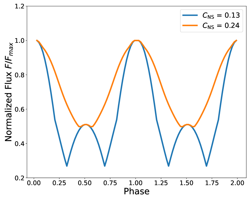
Figure 7: Comparison between the pulsed profiles of two NSs with the same radius, $R_{\rm NS}=11\,\rm km$, but a different compactness, $C_{\rm NS}$ (see Eq. (19)), of $0.13$ (blue) and $0.24$ (orange), respectively. In this example, both stars are characterized by two antipodal, circular hot spots with temperatures of $1\,\rm keV$ and sizes of $1\,\rm deg$ and $3\,\rm deg$, respectively. The larger spots generate the higher peaks in the profile, while the smaller ones result in the lower peaks. In both simulations, the LOS and the spot centers form an angle of $90^{\circ}$ with respect to the rotational axis. We observe that an increase in the compactness widens the pulse profiles and decreases the amplitude of pulsations. The lightcurves were modeled with software presented in [223].

On one hand, the mass enters the picture through the compactness parameter (Sec. 3.5), which controls the level of light bending. Specifically, light bending allows the hot spots to be visible even if they are located on the back of the star, facing away from the observer. This effectively reduces the amplitude of the pulsed lightcurve (i.e., the difference between the peak and the minimum of the flux; see Fig. 7 for an illustration). On the other hand, the radius plays a role not only via the compactness but also through the Doppler effect, which is mass independent and causes an asymmetry in the pulse profile due to the stellar rotation. At a fixed angular velocity, a larger NS has a higher surface velocity and, consequently, shows a stronger Doppler boost of the hot-spot emission. This influences the shape of the pulses, making them more asymmetric. Moreover, as the asymmetry becomes more pronounced for fast rotators, MSPs are the ideal candidates for constraining the radius with this kind of analysis [175]. We note that although this method can constrain the mass and radius at the same time, an independent measure of the mass (through any of the methods outlined in Sec. 3.1) leads to tighter constraints on the radius [e.g., 224].

This technique, which is based on spectro-timing observations, is more robust than the spectral approaches presented earlier, because it is less affected by systematic errors. The primary assumption made here concerns the propagation of photons in the atmosphere, which is typically assumed to be non-magnetized and composed of fully ionized hydrogen (or helium). This implies that the magnetic field has a negligible effect on the propagation of photons and that the primary sources of opacity are free-free absorption and electron scattering [225]. This is justified for MSPs, which are characterized by the weakest magnetic fields in the NS population (see Fig. 1). Another approximation that is usually made to ray-trace the photons from the stellar surface to the observer is the so-called oblate Schwarzschild plus Doppler approximation [219], which improves on the Schwarzschild plus Doppler approximation [215, 217] by including the rotation-induced oblateness of the star. This is particularly important for rotational frequency above $300\,\mathrm{Hz}$, where the oblateness leaves a measurable imprint on the lightcurve [226]. In this approximation, the rotation determines the NS ellipticity and the Doppler boosting of light, but it has no impact on the spacetime metric, which is taken to be the Schwarzschild metric. This last assumption is justified because the NS mass quadrupole has little effect on the metric and gravitomagnetic effects are generally negligible [216, 227, 219, 220]. Nevertheless, effects induced by quadrupolar deformations and rotation can also be included [e.g., 228, 229].

The main difficulty with this method lies in the degeneracy between the many parameters it employs. These include, in addition to the stellar mass and radius, the source distance, the hydrogen column density, $N_{H}$, as well as the parameters needed to describe the surface temperature map, along with the angles encoding the orientation of this map with respect to the rotational axis and the observer’s LOS. Low counts in the detected lightcurve or noisy data can lead to degeneracies between the model parameters or multi-modal posteriors, resulting in significant uncertainties in the mass and radius estimates [230].

These issues have significantly improved in recent years due to the unprecedented sensitivity of NASA’s Neutron Star Interior Composition Explorer (NICER) [231], installed on the International Space Station in 2017. In particular, NICER has allowed radius constraints for the MSPs PSR J0030+0451 [229, 232, 230] and J0740+6620 [224]. Analysis of the former led to $R_{\rm NS}=12.71^{+1.14}_{-1.19}\,\textrm{km}$ and $M_{\rm NS}=1.34^{+0.15}_{-0.16}\,M_{\odot}$ at $68\%$ credibility level [229] (corresponding to a relative error $<10\,\%$), which is consistent with an independent analysis by [232]. Whereas PSR J0030 is an isolated NS, PSR J0740 is in a binary system and exhibits a favorable inclination which allowed a mass measurement via Shapiro delay (see Sec. 3.1.2), leading to $M_{\rm NS}=2.08^{+0.07}_{-0.07}\,M_{\odot}$ [67]. As discussed above, the independent measurement of the mass allowed for an improved radius constraint for this source, resulting in $R_{\rm NS}=12.39^{+1.30}_{-0.98}\,\textrm{km}$ [224].

Although retaining a certain level of model dependence and degeneracies between parameters (leading us to classify pulse profile modeling as yellow in Tab. 2), we consider this technique the most promising in providing accurate and precise constraints on the NS radius in the coming years.

We conclude by highlighting that pulse profile modeling, which also allows us to infer information about the geometry of the hot spots, encodes NS information beyond the mass and the radius. In particular, hot-spot properties are related to the geometry of the NS’s magnetic field [233]. Analyses of NICER data for both MSPs discussed above disfavored a simple dipolar poloidal magnetic field configuration, which has implications for the magnetospheric structure and emission mechanisms [234, 235, 236, 237].

3.2.4 Multi-messenger observations of neutron star-black hole mergers

Multi-messenger observations of CBMs provide a new channel to measure the NS radius. For this task, NS- black hole (BH) systems are the optimal targets due to their relative simplicity with respect to BNS systems. Such a NS-BH merger has two possible outcomes. Either the NS plunges directly into the BH, or it is tidally disrupted outside the BH’s innermost stable circular orbit (ISCO) [238, 239, 240, 241, 242, 243]. In the second case, an accretion disk forms around the BH. The resulting system may launch a relativistic jet, which is able to power a short-duration GRB, one of the most luminous transients in the Universe [244, 245, 246] (for recent reviews about CBMs and their EM counterparts see [247, 248]). GRB emission consists of the highly variable prompt emission, observable in gamma-rays and powered by the dissipation of kinetic energy within the jet (internal dissipation), which is followed by a multi-wavelength afterglow due to the dissipation of jet energy in the interstellar medium (external dissipation). For an accretion-powered jet, the corresponding GRB energy, $E_{\rm GRB}$, is proportional to the mass, $M_{\rm disk}$, of the accretion disk with a proportionality constant, $\epsilon_{\rm jet}$, that is referred to as the jet-launching efficiency. This quantity depends on the efficiency of converting the accreted mass into the jet’s kinetic energy and the efficiency of converting the latter into radiation. In the case of a NS-BH merger, we can express $M_{\rm disk}$ as a (semi-analytical) function of relevant system parameters, specifically the masses, $M_{\rm NS}$ and $M_{\rm BH}$, of both objects, the NS radius, $R_{\rm NS}$, and the dimensionless BH spin parameter, $a_{\rm BH}$ [249]. As a result, we obtain

$$E_{\rm GRB}=\epsilon_{\rm jet}M_{\rm disk}(M_{\rm NS},M_{\rm BH},a_{\rm BH},R_{\rm NS}).$$ (24)

Whereas we can measure $E_{\rm GRB}$ from EM observation (typically in the gamma-ray and X-ray bands for the prompt emission and afterglow, respectively), $M_{\rm NS}$, $M_{\rm BH}$ and $a_{\rm BH}$ are deduced from the parameter estimation of the GW signal. By estimating $\epsilon_{\rm jet}$, or defining a reasonable prior distribution (typical values deduced from theoretical models [250, 251, 252, 253, 254, 255, 256] and observations of GW170817 [257] fall in the range of $10^{-4}-10^{-1}$; see Tab. 1 of [257] for a summary), we can then solve Eq. (24) for $R_{\rm NS}$. Assuming an SNR of $10$ for the GW detection, [258] use this method to deduce that we can measure the radius with a relative uncertainty $<20\%$ at $90\%$ confidence (see [259] for a conceptually similar approach).

However, this method suffers from several assumptions. The most important one concerns our lack of detailed knowledge of the efficiency, $\epsilon_{\rm jet}$. Second, the above picture does not consider that these accretion disks can lose on the order of $10\%$ of their mass through winds [e.g., 260, 261].

It is also worth adding that while NS-BH mergers are possible short GRB progenitors, they are likely only responsible for a minority of the short GRB population, whose bulk is produced by BNS mergers [262]. Moreover, NS-BH mergers are not particularly promising multi-messenger sources, because the tidal disruption of the NS outside the BH ISCO is not particularly likely [263]. Consequently, we consider this method of extracting $R_{\rm NS}$ as strongly model dependent, classifying it as orange in Tab. 2. However, once the NS radius has been tightly measured, this approach could be of great interest in constraining the uncertain jet-launching efficiency, $\epsilon_{\rm jet}$.

We finally note that the above concept can, in principle, also be used in association with BNS mergers and exploit not only GRBs but also other associated transients such as KNe (see also Sec. 3.9.1). [264], for example, developed a fitting formula for the BNS-merger dynamical ejecta (which contributes to fuel the kilonova emission) similar in concept to the formula for $M_{\rm disk}$ discussed above. However, considering BNS systems does not reduce the level of model dependence but rather increases it due to the higher complexity of the binary.

3.2.5 Gravitational-wave asteroseismology

This method (classified as yellow in Tab. 2) is the same as that presented in Sec. 3.1.4 to measure the mass of a NS. We remind the reader that the main idea is to exploit quasi-universal relations linking the frequency and damping time of some particular quasi-normal mode (such as the $f$-mode or $w$-modes) with the NS mass and radius to constrain both parameters.

In addition to the discussion in Sec. 3.1.4, we present here another method to exploit asteroseismology to measure NS radii in the context of BNS mergers. The general idea is based on the fact that a NS (either stable or metastable) formed as a consequence of the binary coalescence will emit GWs through the excitation of quasi-normal oscillations [265, 266, 267, 268, 269, 270]. Although faint, this post-merger signal should be detectable for a merger occurring at a distance of a few up to a few tens of Mpc with second-generation interferometers [e.g., 271, 272, 273, 274], while many such detections are expected for third-generation facilities [e.g., 275, 276]. In particular, the spectrum of the post-merger signal is characterized by several peaks, whose characteristic frequencies are associated with different properties of the NS remnant through quasi-universal relations. These relations, for example, allow us to extract the radius of a non-rotating neutron star with maximum mass [266] or the stellar compactness [267, 268, 277]. Therefore, detecting post-merger signals and measuring the corresponding characteristic frequencies provides a wealth of information about dense-matter physics and could, e.g., constrain possible quantum-chromodynamics phase transitions between hadronic and quark matter in hybrid stars [e.g., 278, 279, 280, 281].

Moreover, [282] pointed out that a measurement of the compactness via the aforementioned quasi-universal relations could be combined with a measurement of the system’s total mass as derived from the inspiral phase to obtain an estimate of the NS radius. [282] underlined that, although the uncertainty on the measured frequency would be too large to obtain meaningful radius constraints for a single detection with second-generation interferometers (since sources at distances of $\sim 200\,\mathrm{Mpc}$ are characterized by SNRs $<1$), the joint uncertainty of $\sim 100$ BNS detections could provide an average measurement on the radius with an uncertainty of $\sim 2-12\,\%$. In this case, larger uncertainties were associated with softer EOSs.

3.3 Moment of inertia

Method	GWs	Radio	Optical	X-ray	$\mathbf{\gamma}$-ray
Relativistic spin-orbit coupling
Pulsar glitches
Continuous GWs
GW asteroseismology

Table 3: Moment of inertia measurements. Individual rows represent the methods that provide NS moments of inertia, while columns denote different messengers/EM wavebands. Individual colors are equivalent to those in Tab. 1.

We next turn to techniques, summarized in Tab. 3, that constrain the NS’s moment of inertia, $I_{\rm NS}$. The quantity’s importance lies in the fact that a measurement of $I_{\rm NS}$, coupled with a mass measurement, directly allows constraining the dense-matter EOS and the NS radius [44, 283], bypassing an independent measurement of $R_{\rm NS}$, which is generally affected by significant model dependencies and systematics (see Sec. 3.2). We also point out that since $I_{\rm NS}\propto M_{\rm NS}R_{\rm NS}^{2}$ (i.e., the moment of inertia depends on $R_{\rm NS}$ squared), the range of moment of inertias for different EOSs is larger than the range of viable NS radii [44]. Consequently, $I_{\rm NS}$ measurements make constraining the EOS easier than $R_{\rm NS}$ measurements.

We note that in what follows $I_{\rm NS}$ is associated with a fiducial moment-of-inertial value unless stated otherwise.

3.3.1 Relativistic spin-orbit coupling

In GR, the spins of two bodies in a compact binary are coupled with each other and their orbital motion [284, 285]. As the orbital angular momentum represents the dominant contribution to the total angular momentum, spin-spin coupling is weaker than spin-orbit coupling and can be safely neglected [44]. However, relativistic spin-orbit coupling, also known as Lense-Thirring precession, drives an advance of the orbit’s periastron in addition to the post-Keplerian contributions introduced in Sec. 3.1.1. Spin-orbit coupling also causes the orbital angular momentum vector to precess around the total angular momentum, which in turn drives precession of the objects’ spins due to angular momentum conservation [286, 44]. As the orbital angular momentum dominates over the spins, the former contribution is generally small, while precession of the spins can be substantial. However, both effects are detectable in BNS systems via radio timing if one or both of the stars are pulsars [287, 288, 289].

The predicted evolution of the two spins, $\mathbf{S}_{i}$, and orbital angular momentum, $\mathbf{L}$, due to spin-orbit coupling is [284]:

$$\dot{\mathbf{S}}_{i} =\frac{G(4M_{i}+3M_{-i})}{2M_{i}a^{3}c^{2}(1-e^{2})^{3/2}}\,\mathbf{L}\times\mathbf{S}_{i},$$ (25)

$$\dot{\mathbf{L}} =\sum_{i}\frac{G(4M_{i}+3M_{-i})}{2M_{i}a^{3}c^{2}(1-e^{2})^{3/2}}\,\left(\mathbf{S}_{i}-3\frac{\mathbf{L}\cdot\mathbf{S}_{i}}{|\mathbf{L}|^{2}}\mathbf{L}\right),$$ (26)

where we follow [44] and denote the two binary components with subscripts $i={\rm A,B}$ and $-i={\rm B,A}$, respectively. The resulting precession periods of both objects are [44]

$$P_{{\rm precession},\,i}=\frac{2c^{2}aP_{\rm orb}M(1-e^{2})}{GM_{-i}(4M_{i}+3M_{-i})}.$$ (27)

Equations (25) and (26) highlight that spin and orbital plane precession occur only when the spins and orbital angular momentum are misaligned. If this is the case, the change in geometry should lead to a time-varying pulse profile [290] (and potentially the disappearance and reappearance of the pulsar radiation [44]) plus a variation in the orbital plane’s orientation. The latter manifests itself as a change in the inclination, $i$, [285] and is, thus, observable as a variation in the projected semi-major axis, provided the binary is not observed edge-on (i.e., $\sin i\nsim 1$). If, in addition, one pulsar spins much faster than the other, its spin will provide the dominant contribution to the spin-orbit coupling, and the observed effect depend directly on its moment of inertia as $|\mathbf{S}|=I_{\rm NS}\Omega$, where $\Omega=2\pi/P$ is the star’s angular velocity.

For alignment between the spins and the orbital angular momentum, we instead obtain $\dot{\mathbf{S}}_{i}=0$ and $\dot{\mathbf{L}}\propto-\sum_{i}\mathbf{S}_{i}={\rm const}$. This implies that only the periastron motion is present, which, in turn, occurs in the opposite direction to the orbital motion. Moreover, if $|\mathbf{S}_{\rm A}|\gg|\mathbf{S}_{\rm B}|$, the resulting effect is again dependent on the moment of inertia of pulsar A and a corresponding measurement would, therefore, also constrain the NS moment of inertia [e.g., 291, 44, 290, 97].

Extracting changes in inclination angle, $i$, for known BNSs with sufficiently high precision poses significant challenges [e.g., 292]. As a result, $I_{\rm NS}$ constraints from the periastron advance are currently more promising. In particular, the Double Pulsar PSR J07037–3039A/B [293, 294, 97], a system whose orbit is seen almost edge-on, pulsar A rotates much faster than pulsar B and spin A is almost parallel to $\mathbf{L}$, is a promising target for this method. Accounting for future observations with MeerKat and the Square Kilometre Array, [290] predict a moment-of-inertia measurement for the Double Pulsar with $11\%$ accuracy by 2030.

The main limitations of this measurement are threefold. First, relativistic spin-orbit coupling depends on the individual masses of both objects. Consequently, to measure the moment of inertia through periastron advance, we require an independent measurement of the individual binary masses. Moreover, we also require knowledge of the orientation of the pulsar spin with respect to the orbital angular momentum. Third, the periastron advance has a dominant spin-independent contribution that originates from the first and second post-Newtonian correction of the orbital motion (see Sec. 3.1.1). To extract $I_{\rm NS}$, we therefore need to be able to disentangle the spin-orbit contribution to the total periastron advance from the post-Newtonian contribution. Addressing these issues requires a precise measurement of three post-Keplerian parameters, and building up a sufficiently precise pulsar timing solution can take decades. Thus, long-term datasets such as those obtained for PSRs B1913+16 [95], B1534+12 [289] or the Double Pulsar PSR J0737–3039A/B [97] will be crucial to detect this effect (if possible at all). However, a single successful measurement would provide tight moment-of-inertia constraints.

Factoring in these caveats, we classify this method as yellow in Tab. 3.

3.3.2 Pulsar glitches

Another phenomenon that indirectly probes the NS moment of inertia are so-called pulsar glitches, sudden spin-ups that interrupt the otherwise regular electromagnetic NS spin-down. High-precision timing of glitching pulsars with radio telescopes allows us to quantify the size of these glitches as well as the shape of the signal on timescales of minutes to months [e.g., 295, 296, 297, 298, 299, 300]. Glitches have also been observed in the X-rays and gamma-rays although generally with lower precision [e.g., 301, 302, 303]. As a result, we know that glitches are common in isolated pulsars and more than 650 spin-ups have now been observed in over 200 NSs [296, 307], providing ample opportunity to probe related physics.

Glitch amplitudes vary between $|\Delta\Omega|/\Omega\sim 10^{-12}-10^{-5}$, where $|\Delta\Omega|$ is the size of the glitch. Those pulsars exhibiting large glitches repeatedly (such as the Vela pulsar [295, 308, 298]) are of particular interest for $I_{\rm NS}$ considerations, as sudden spin-ups in these objects are associated with the presence of internal superfluids. We refer to Sec. 3.8 for details on the microscopic aspects of superfluidity and focus on the macroscopic implications here.

Superfluid models explain glitches by the rapid transfer of angular momentum from an internal, differentially rotating superfluid (decoupled as a result of vortex pinning) to the rest of the star [e.g., 309, 310, 311, 312, 313]. The superfluid interpretation is crucial for giant glitches, as the star-quake model (an alternative explanation based on the build up of strain in the NS crust, analogous to Earth quakes [314, 315, 316]) cannot provide sufficient stresses to explain frequent, Vela-like glitches. We will, thus, focus on the superfluid framework here.

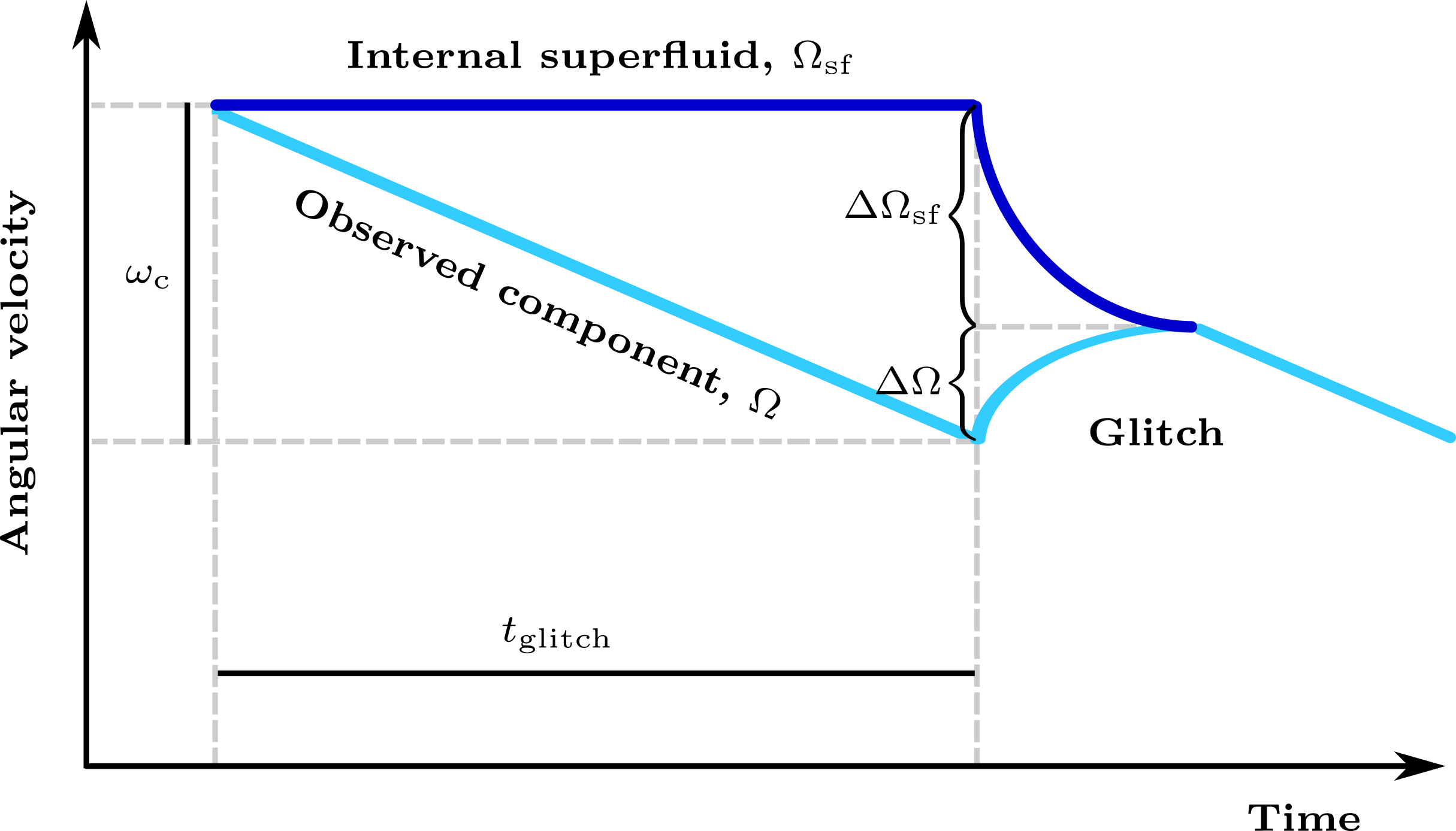
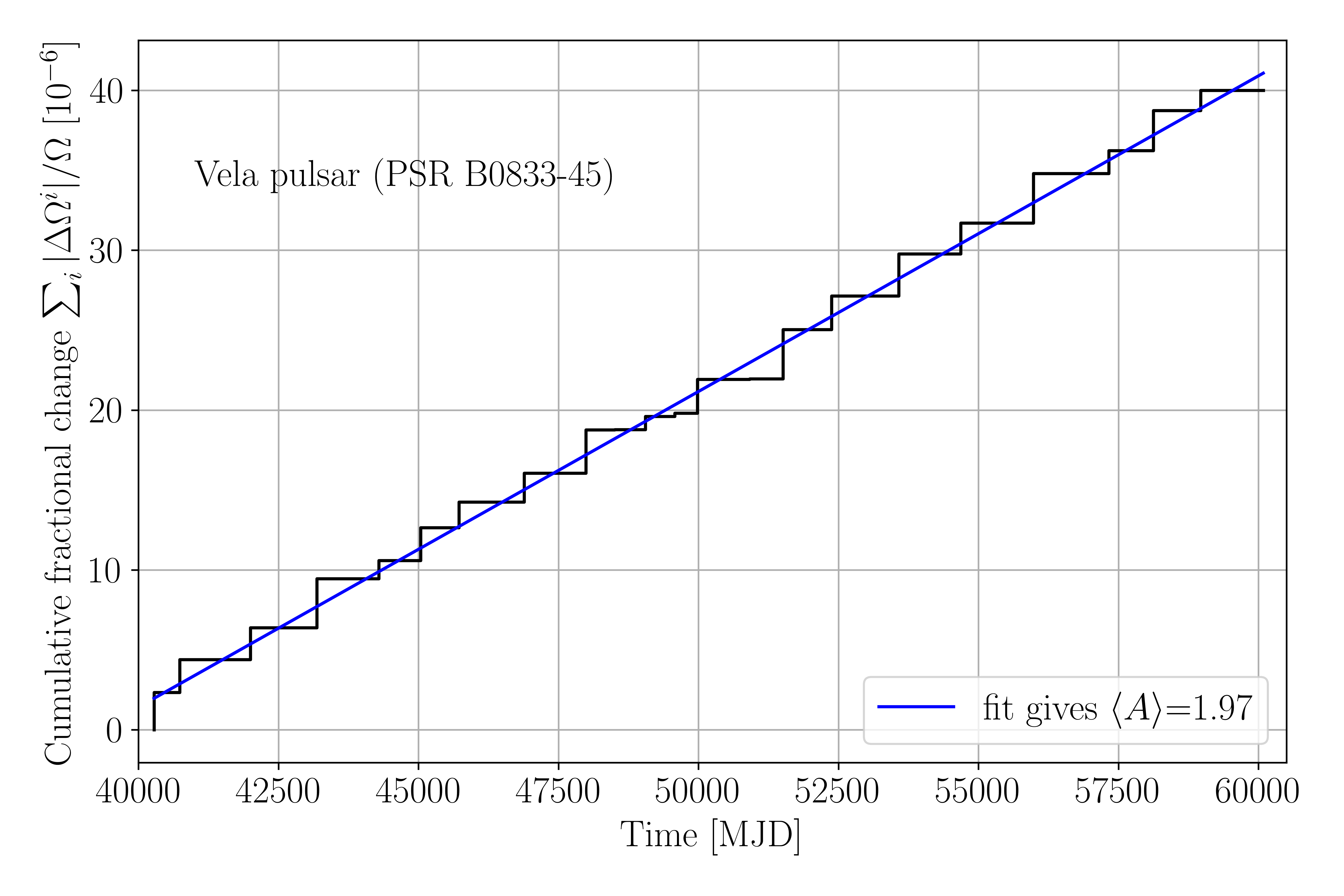
Figure 8: Illustrating the pulsar glitch phenomenon. Top panel: Sketch of the physics underlying a glitch in the so-called two-component model and relevant quantities used in the text. An internal superfluid is decoupled from the observed component, spinning down due to the loss of electromagnetic energy. At a critical lag, $\omega_{\rm c}$, both recouple, causing the observed component to spin up, producing the glitch. Bottom panel: Cumulative fractional change of spin frequency caused by glitches in the Vela pulsar PSR B0833–45 over time. The straight blue line is the least-squared fit to the data, whose slope is equivalent to the average glitch activity parameter, $\langle\mathcal{A}\rangle$. The corresponding value of $\langle\mathcal{A}\rangle=1.97$ leads to an inferred superfluid fraction of $I_{\rm sf}/I_{\rm NS}=2\tau_{\rm c}\langle\mathcal{A}\rangle=1.63\%$. Glitch data are taken from [307].

Interpreting glitches in a two-component picture (shown in the top panel of Fig. 8) and assuming complete depletion of the superfluid reservoir, angular momentum conservation dictates

$$I_{\rm sf}\Delta\Omega_{\rm sf}=I_{\rm obs}|\Delta\Omega|.$$ (28)

Here, $I_{\rm sf}$ denotes the superfluid’s moment of inertia, $\Delta\Omega_{\rm sf}$ the change in its angular velocity, and $I_{\rm obs}$ the moment of inertia of the observed component undergoing the glitch, i.e., $I_{\rm sf}+I_{\rm obs}=I_{\rm NS}$. As both components recouple during the glitch and then corotate, Eq. (28) can be rewritten in terms of the velocity lag, $\omega_{\rm c}\equiv\Omega_{\rm sf}-\Omega$, at the time of the glitch, which itself depends on the interglitch time, $t_{\rm glitch}$, and characteristic age, $\tau_{\rm c}$ (see Fig. 8 and [317] for details). While this, in principle, allows us to determine $I_{\rm sf}/I_{\rm NS}$ for pulsars with at least two large glitches, interglitch times and sizes differ significantly between events for any given pulsar [e.g., 296, 297, 299, 300]. We thus define an average glitch activity parameter, $\langle\mathcal{A}\rangle$, for pulsars exhibiting $N$ spin-ups in an observation period, $t_{\rm obs}$. $\langle\mathcal{A}\rangle$ can be directly measured from observations (see bottom panel of Fig. 8) and leads to

$$\frac{I_{\rm sf}}{I_{\rm NS}}\approx 2\tau_{\rm c}\,\frac{1}{t_{\rm obs}}\,\sum_{i}^{N}\frac{|\Delta\Omega^{i}|}{\Omega}\equiv 2\tau_{\rm c}\langle\mathcal{A}\rangle.$$ (29)

Corresponding estimates for $I_{\rm sf}/I_{\rm NS}$ range from $0.5$ to a few percent [e.g., 318, 317], which can be compared to the moment of inertia of the neutron superfluid in the NS’s inner crust. This region is typically considered as the origin of pulsar glitches, because vortices can directly pin to crustal lattice structures, naturally explaining the superfluid’s decoupling. For standard EOSs and NS mass ranges, the inner crust constitutes between $\approx 2-8\%$ [e.g., 318, 317] of the star’s total moment of inertia, thus supporting the crust-origin interpretation of pulsar glitches.

Recent results [317, 319], however, suggest that Eq. (29) does not account for the fact that crustal neutrons might be difficult to move due to so-called entrainment [320, 321], effectively reducing the available moment of inertia. While still uncertain [e.g., 322, 323], if entrainment is indeed present, [317] estimate that the right-hand-side of Eq. (29) needs to be modified by an additional factor $\sim 4.3$. For some glitching NSs, this would imply that the crustal superfluid no longer holds sufficient moment of inertia to explain large and frequent glitches, as for example observed in the Vela pulsar. This in turn can also set constraints on the underlying EOSs, NS masses and radii [324]. Further assumptions on the interactions of individual vortices allow us to set additional constraints on NS masses as, e.g., suggested by [325].

In conclusion, glitches provide indirect evidence on the moments of inertia of the components involved in the spin-up process and some insights into the EOS, NS masses, and radii. However, estimates (although readily available due to the abundance of glitch observations) are strongly model dependent as shown in Tab. 3. The above framework, for example, assumes that glitches are linked to the presence of superfluidity, NSs are composed of two interacting components, and the superfluid angular momentum reservoir is completely depleted during the spin-up. A better understanding of the glitch process and improved theoretical models will be needed to take further advantage of these spin-ups to provide advanced constraints on the NS moment of inertia.

3.3.3 Continuous gravitational waves

Rotating NSs emit GWs at the expense of their rotational energies. A time variation in the mass quadrupole moment can, for example, be produced by a tri-axial star rotating rigidly about a principle axis or an axisymmetric (bi-axial) body whose rotation axis does not coincide with the symmetry axis (see [326, 327] for recent reviews). Whereas in the former case, continuous GWs are emitted at a frequency $2\Omega$, the latter case also produces GW emission at $\Omega$, which dominates over the harmonic at $2\Omega$ in the limit of small angles between the rotation and the symmetry axis [328]. Emission of GWs at both $\Omega$ and $2\Omega$ can furthermore occur due to magnetic-field induced stellar distortions [329] or the presence of superfluid components [330]. Although current GW detectors may not yet be sensitive enough to directly detect these signals (physically interesting limits on NS properties have however been obtained with current facilities as we outline in Sec. 3.7.3), third-generation interferometers have the strong potential to detect continuous GWs. We will, thus, focus on the $2\Omega$-case, which applies to non-axial NSs, e.g., those that support a mountain (see also Sec. 3.7.3 for details). Such a star loses energy at the rate [113]

$$\dot{E}\approx-\frac{32G}{5c^{5}}I_{3}^{2}\varepsilon^{2}\Omega^{6},$$ (30)

where $I_{3}$ is the moment of inertia along the rotation axis, $\varepsilon\equiv(I_{2}-I_{1})/I_{3}$ the ellipticity and $I_{1},I_{2}$ denote the moments of inertia in the directions orthogonal to the rotational axis. Note that these moments of inertia can vary from the fiducial value, $I_{\rm NS}$, by a factor of a few. The corresponding NS spin-down is, thus, characterized by

$$\dot{\Omega}\approx-\frac{32G}{5c^{5}}\Omega^{5}\varepsilon^{2}I_{3},$$ (31)

while the continuous GW emission has the amplitude [331]

$$h_{0}\approx\frac{4G}{c^{4}}\frac{1}{D}I_{3}\varepsilon\Omega^{2},$$ (32)

for a source at distance, $D$.

[332] recently developed a method to measure the moment of inertia of a NS from this continuous GW emission. The method is simple in concept and exploits the quasi-standard siren nature of GW-emitting NSs, taking advantage of the fact that Eqs. (31) and (32) contain the measurable quantities $h_{0},\Omega$, and $\dot{\Omega}$. Although these two relations provide insufficient information to constrain the three unknowns $\varepsilon,I_{3}$, and $D$, we can combine both equations to eliminate the ellipticity and relate $\sqrt{I_{3}}/D$ to our observables:

$$\frac{\sqrt{I_{3}}}{D}=\sqrt{\frac{2c^{3}}{5G}}\sqrt{\frac{\Omega}{|\dot{\Omega}|}}\,h_{0}.$$ (33)

If, in addition, we have an independent way to measure $D$, we could directly constrain the moment of inertia. Unfortunately, measuring NS distances is a difficult task [175]. In particular, since the NSs that we currently observe only constitute a very small fraction of the total NS population [333, 334, 335], several continuous GW sources that will be detected by future GW interferometers will lack an EM counterpart. This will likely make a determination of distances even more challenging. In such cases, it might however be possible to constrain the source’s distance by extracting its parallax directly from the GW signal [336]. This would allow us to break the degeneracy between $I_{3}$ and $D$, and infer the moment of inertia using continuous GW observations only. Our ability of measuring the GW parallax increases with larger observation span, SNR and NS spin frequency [336]. For example, [336] identify a NS rotating at $400\,\rm Hz$ observed in the GW band with an $S/N\sim 100$ for $1\,\rm yr$ as the best case scenario, and suggest the source’s parallax can be measured if it is located within $100\,\rm pc$ from Earth.

We can translate the concepts outlined for tri-axial stellar deformations to the continuous GWs emission by so-called $r$-modes. $r$-modes are toroidal oscillation modes expected in rotating NSs, where the Coriolis force acts as the restoring force [337] (see [338] for a review). They are the NS analog of Rossby waves in the Earth’s oceans [339]. One important point concerning $r$-modes is that they are expected to be subject to the so-called Chandrasekhar-Friedman-Schutz (CFS) instability [340, 341]. This instability occurs in rotating stars when rotation is so fast that a counter-rotating oscillation mode in the rotating frame appears to co-rotate in the laboratory frame. In this case, GW emission subtracts angular momentum from the mode. However, as the mode’s angular momentum is negative in the rotating frame, this subtraction increases the absolute value of the angular momentum of the mode. As a result, the emission of GWs does not damp the mode, but instead causes it to grow. We note, however, that while the $r$-mode satisfies the CFS instability criterion under the assumption of a perfect fluid star, other dissipative effects such as shear or bulk viscosity can damp or even stop the instability [e.g., 342]. As a result, complex microphysics [see, e.g., 343, 344] determine the highly uncertain saturation point to which the $r$-mode amplitude can grow. Nonetheless, GW emission driven by the $r$-mode would be continuous at the expense of the star’s rotational energy.

Focusing on the lowest-order Newtonian $r$-mode (characterised by the spherical harmonics $l=m=2$, where $l$ and $m$ denote the degree and order of the corresponding Legendre polynomial, $P_{l}^{m}$, respectively) for an incompressible, barotropic star, we can write the corresponding GW strain amplitude as [345]

$$h_{0,r}=\sqrt{\frac{8\pi}{5}}\frac{G}{c^{5}}\frac{1}{D}\alpha M_{\rm NS}R_{\rm NS}^{3}\tilde{J}\omega^{3}_{r}.$$ (34)

Here, $\alpha$ is the dimensionless quantity that parameterizes the saturation amplitude [346], the dimensionless parameter $\tilde{J}$ depends on the NS’s mass-density profile (see, e.g., Eq. (6) in [332]), and $\omega_{r}\simeq 4\Omega/3$ is the $r$-mode’s angular frequency.

Assuming that all the energy associated with the excitation of $r$-modes is lost through GWs, we obtain the following spin-down formula:

$$\dot{\Omega}=-\frac{218\pi G}{3852c^{7}}\,(\alpha M_{\rm NS}R_{\rm NS}^{3}\tilde{J})^{2}\,\frac{\Omega^{7}}{I_{3}}.$$ (35)

Similar to what we discussed above, we can now combine the previous two equations to eliminate the factor $(\alpha M_{\rm NS}R_{\rm NS}^{3}\tilde{J})$ and solve for the ratio $\sqrt{I_{3}}/D$ to obtain:

$$\frac{\sqrt{I_{3}}}{D}=\sqrt{\frac{8c^{3}}{45G}}\sqrt{\frac{\Omega}{|\dot{\Omega}|}}\,h_{0,r}.$$ (36)

By measuring observable quantities, we can, therefore, again constrain the stellar moment of inertia.

The underlying assumption of this technique concerns the use of Eqs. (31) and (35). Both relations assume that the observed spin-down is dominated by a specific type of continuous GW emission. However, pulsar observations show that this is generally not satisfied, as a number of other processes can spin down a rotating NS. These are characterized by the so-called braking index, $n$, which encodes the exponent of $\Omega$ in relations of the form $\dot{\Omega}\propto\Omega^{n}$. For pulsars with precise timing solutions, it can be obtained via

$$n\equiv\frac{\Omega\ddot{\Omega}}{\dot{\Omega}^{2}}.$$ (37)

See [299] for a recent overview of measured braking indices and corresponding systematics. From Eq. (31), we, hence, deduce that $n=5$ for pulsars that slow down due to GW emission from a mountain, and $n=7$ if GWs are emitted due to $r$-modes. In turn, $n=3$ characterizes a NS that spins down due to magnetic dipole emission, which we discuss in more detail in Sec. 3.6.1. Consequently this method only applies to those cases, where $n=5$ or $n=7$ is observed, significantly reducing the number of potential targets for moment-of-inertia measurements, because most pulsars exhibit $n<3$. However, we note that EM observations of the young X-ray pulsar PSR J0537–6910 hint at an $n=7$ spin-down [347]. As the NS’s distance is known, the source is a prime candidate for searches of continuous GWs from $r$-modes [327], which have started to probe relevant parameter spaces [348].

Recently, [349] extended the approach of [336] to also account for the dipole spin-down emission. This generalization, which introduces another parameter, i.e., the magnetic dipole moment, however requires an additional measurement to constrain the NS moment of inertia. [349] focus on the second derivative of the rotational frequency, $\ddot{\Omega}$. As a result, their method is not restricted to sources with $n=5$ only, but to those with $n\in[3,5]$. However, also in this case, knowledge of the distance is required. In particular, [349] estimate that the relative uncertainty on the moment of inertia will be limited to $27\%$ with increasing observation time for a relative distance uncertainty of $20\%$.

Finally, we note that $n=5$ is not exclusive to quadrupolar GW spin down, but also characterizes braking by magnetic quadrupole radiation. This would, however, require a magnetic-field configuration where the quadrupole component dominates over the dipolar one, for which we currently do not have observational evidence.

As a result of these restrictions, we classify this method as somewhat model dependent in Tab. 3.

3.3.4 Gravitational-wave asteroseismology

GW asteroseismology, already discussed in Sec. 3.1.4 for the NS mass, provides a valuable method to measure the moment of inertia of a NS, which we classify as somewhat model dependent in Tab. 3. Besides the quasi-universal relations presented previously, [120] found another universal relation for the $f$-mode that links the frequency and the damping time of the mode to the mass and moment of inertia, instead of $M_{\rm NS}$ and $R_{\rm NS}$. While the relation from [120] holds for non-rotating stars, generalizations for the case of rapid rotation have also been found [350, 351]. We specifically note that these relations appear to be tighter for the range of possible EOSs than those relations involving mass and radius. On top of that, the relation in [120] also holds for quark stars. However, as outlined in Sec. 3.1.4, the main issue of this method currently concerns the detectability of GW waves from quasi-normal modes with present facilities, and the accuracy required for measuring mode frequencies and damping times to constrain NS parameters. Third-generation interferometers may finally allow for an exploration of this technique [352, 353].

3.4 Tidal deformability

Method	GWs	Radio	Optical	X-ray	$\mathbf{\gamma}$-ray
Tidal deformability in CBMs
GW asteroseismology

Table 4: Tidal-deformability measurements. Individual rows represent the methods that provide the tidal deformability of NSs, while columns denote different messengers/EM wavebands. Individual colors are equivalent to those in Tab. 1.

Our fourth parameter of interest is the tidal deformability of NSs, a quantity which directly relates to the dense-matter EOS. In a compact binary system composed of a NS and a companion, which we require to be another NS or a low-mass BH for this parameter to be measurable (see below), the NS is subject to the tidal field of its companion. The quadrupolar contribution to this tidal field is given by [113, 354]:

$$\mathcal{E}_{ij}=c^{2}R_{0i0j},$$ (38)

where $R_{\mu\nu\rho\sigma}$ is the Riemann tensor. This tidal field perturbs the NS and induces a quadrupole moment, which is proportional to the field itself:

$$Q_{ij}=-\lambda_{\rm NS}\mathcal{E}_{ij}.$$ (39)

The constant of proportionality, $\lambda_{\rm NS}$, is a dimensional quantity encoding information about the NS’s properties referred to as the tidal deformability. It is typically expressed in terms of the NS radius and another dimensionless quantity, the l=2 tidal Love number, $k_{2}$, (where $l$ denotes the degree of the corresponding spherical harmonic) through [113, 354]

$$\lambda_{\rm NS}=\frac{2k_{2}R_{\rm NS}^{5}}{3G}.$$ (40)

The tidal Love number depends on the dense-matter EOS. For realistic choices of EOS, it ranges between $k_{2}\simeq 0.05-0.15$, with lower values corresponding to softer EOSs [113]. Thus, by measuring $\lambda_{\rm NS}$, it is possible to constrain the EOS.

In the following, we will provide a brief overview of how the tidal deformability can be measured from observations of GWs. For a more detailed discussion of the topic, we refer the interested reader to [355, 356, 113, 354].

Finally, we also mention the existence of universal relations between the moment of inertia, the tidal Love numbers, and the NS’s quadrupole moment. These relations, known as I-Love-Q relations, express either of these three quantities as a function of one of the other two. These relations, thus, allow us to obtain the remaining two quantities when one of them is measured [357]. For example, a measurement of the moment of inertia, performed with one of the methods presented in Sec. 3.3, can be used to infer the tidal Love number through a relation between the moment of inertia and the Love number [358]. Vice versa, if the tidal Love number is constrained in a compact binary merger, as explained in the next section, we can use this information to constrain the star’s moment of inertia and the quadrupole moment [358].

3.4.1 Compact-binary mergers

GW signals from BNS or NS-BH mergers are sensitive to the tidal deformability, because the quadrupole moment induced in the NS by its companion provokes an increase in the emission of GWs. This effectively results in a faster decay of the orbit compared to a scenario that approximates the merging bodies as point masses. This effect, however, becomes relevant only when the two objects are close to merger, i.e., in the last orbits of the inspiral phase. As the orbital frequency at this stage reaches values around $200\,\textrm{Hz}$, tidal effects are generally observed only in the GW signal above $\sim 400\,\mathrm{Hz}$, where they lead to a correction in the evolution of the GW phase at the 5th post-Newtonian (5PN) order. However, from a numerical point of view, tidal effects in CBMs are sufficiently strong to overcome lower-order terms and are, hence, detectable [e.g., 359].

We note, however, that the tidal deformability, $\lambda_{\rm NS}$, does not enter the 5PN-correction directly. Instead, this correction depends on the quantity

$$\tilde{\Lambda}=\frac{16}{13}\frac{(M_{\rm NS}+12M_{\rm c})M^{4}_{\rm NS}\Lambda_{\rm NS}+(M_{\rm c}+12M_{\rm NS})M^{4}_{\rm c}\Lambda_{\rm c}}{(M_{\rm NS}+M_{\rm c})^{5}},$$ (41)

where $M_{\rm c}$ is again the mass of the companion, while $\Lambda_{\rm NS,\,c}$ are dimensionless quantities related to $\lambda_{\rm NS,\,c}$ through

$$\Lambda_{\rm NS,\,c}=\frac{c^{10}\lambda_{\rm NS,\,c}}{G^{4}M^{5}_{\rm NS,\,c}}.$$ (42)

This quantity takes values between $10-10^{4}$ for realistic NS EOSs and masses, with higher values corresponding to stars of lower mass. For example, for a $1.4\,M_{\odot}$ NS, we obtain a tighter range of $10^{2}-10^{3}$ (see Fig. 1 of [354]). However, if the companion is a BH, then the tidal deformability is typically assumed to be $\lambda_{\rm c}=0$, implying also $\Lambda_{\rm c}=0$. In this case, for a fixed NS mass, $\tilde{\Lambda}$ decreases with increasing BH mass, suggesting that tidal effects are more pronounced, and, thus, easier to measure, when the BH is low in mass.

Equation (41) shows that the measurable quantity $\tilde{\Lambda}$ does not depend on the tidal deformability of a single object, but is instead a linear combination of $\lambda_{\rm NS}$ and $\lambda_{\rm c}$. This degeneracy can be broken by measuring higher-order (i.e., 6PN) terms in the GW [360, 361], which are however unlikely to be detectable with second-generation GW interferometers even for high SNRs of $\sim 30$ [362].

We also note that tidal effects depend on the individual binary masses. We remind the reader that at leading order, the GW signal provides access to a particular combination of the masses known as the chirp mass, $\mathcal{M}$ (see Sec. 3.1.3). Individual masses can be constrained by measuring the next-order terms, which depend on the mass ratio that is, however, degenerate with the spin of both objects. This consequently introduces a (mild) correlation with the spins into the determination of $\Lambda_{\rm NS,\,c}$ and similarly $\lambda_{\rm NS,\,c}$. We consequently classify this method as yellow in Tab. 4.

A measurement of the tidal deformability was possible for the first time with the observation of the BNS merger GW170817. This event allowed us to estimate the parameter $\tilde{\Lambda}$, leading to $\tilde{\Lambda}=300^{+500}_{-190}$ for a low-spin prior (assuming a dimensionless spin parameter $\chi<0.05$) or $<600$ for a high-spin prior ($\chi<0.89$) [1, 363]. An alternative analysis of the same observation produced results that are consistent with these estimates [365]. Ultimately, these insights provided constraints on the NSs’ dense-matter properties, ruling out the stiffest EOSs [363]. Multiple BNS merger detections with third-generation interferometers will improve on these NS EOS constraints [141, 142]. In particular, these detections will allow measurements of $\tilde{\Lambda}$ as well as individual masses through the GW signal providing crucial information on the tidal deformabilities of both merging NSs [366].

3.4.2 Gravitational-wave asteroseismology

In Secs. 3.1.4, 3.2.5, and 3.3.4, we discussed how universal relations enable us to infer the stellar mass, radius and moment of inertia, respectively, from quasi-normal mode frequencies of an oscillating, GW emitting NS. Additional universal relations involving oscillation frequencies and the star’s tidal deformability also exist, allowing us to measure the latter once the corresponding GW signal is detected. In particular, [121] find several relations between the frequency of an $f$-mode of degree $l$ and the tidal deformability of degree $l^{\prime}$ for both NSs and quark stars. Specifically, the cases $l=l^{\prime}$ lead to the most universal, i.e., most EOS-insensitive, relationships. Similar relations have also been discovered in subsequent studies [e.g., 367, 368, 369, 370]. Their origin lies in the combination of the relation between the $f$-mode frequency and the moment of inertia from Sec. 3.3.4 and the above mentioned I-Love-Q relations [121]. Following the same logic as presented in the previous sections on GW asteroseismology, we also classify this method as yellow here.

3.5 Compactness

Method	GWs	Radio	Optical	X-ray	$\mathbf{\gamma}$-ray
Line spectroscopy (redshift)
Pulse profile modeling
Giant-flare QPOs

Table 5: Compactness measurements. Individual rows represent the methods that provide the NS compactness, while columns denote different messengers/EM wavebands. Individual colors are equivalent to those in Tab. 1.

The compactness, $C_{\rm NS}$ (defined in Eq. (19)), measures how densely matter is compressed within the NS volume. Even for the most extreme EOSs, $C_{\rm NS}$ ranges between $0.1$ and $0.3$ [46], whereas causality, i.e., the requirement that the speed of sound must be lower than the speed of light, sets a maximum limit of $C_{\rm NS}=0.354$ [371] (see also Fig. 3).

The main observable imprints (summarized in Tab. 5) directly dependent on this quantity are the gravitational redshift of spectral features and its influence on the bending of photon trajectories. As a result, several methods discussed previously, in particular many of those that provide access to the stellar radius, also lead to compactness constraints. While we will not repeat a discussion of these methods in detail, we briefly mention one which is particularly useful to constrain the compactness. Additionally, we discuss another phenomenon in strongly magnetized NS that might provide independent information on $C_{\rm NS}$.

3.5.1 Line spectroscopy

Observed X-ray spectra of NSs can be permeated by spectral lines due to atomic transitions in regions close to the stellar surface. In particular, in isolated NSs such lines are generated due to absorption in the thin stellar atmospheres. Bright thermally emitting NSs, such as XDINSs, are the most promising targets for such observations (see, e.g., [26] and references therein). Spectral lines are also observed in accreting NSs, where (depending on the viewing geometry) emission and absorption processes in the accretion column or the inner edge of the accretion disk can explain the observed spectral features [372, 373, 374].

Due to the emission/absorption region’s close proximity to the stellar surface, spectral lines can be gravitationally redshifted as a result of the NS’s compactness. More precisely, the gravitational redshift, $z$, is directly related to the stellar compactness by the following equation:

$$1+z\equiv\left(1-2\frac{R_{\rm NS}}{r_{\rm line}}C_{\rm NS}\right)^{-1/2}\simeq\bigl{(}1-2C_{\rm NS}\bigr{)}^{-1/2}.$$ (43)

Here $r_{\rm line}$ is the distance of the line’s origin from the center of the star and the last equality holds if $r_{\rm line}\simeq R_{\rm NS}$. Extracting the redshift via line spectroscopy, thus, in principle, provides a clean and direct way to measure the NS compactness.

However, two issues arise for accreting systems. First, since these sources are usually fast spinning, spectral lines are subject to the Doppler effect, which results in the broadening and distortion of the line profile into an asymmetric shape [372]. This introduces an important systematic in measuring the compactness, which can be as high as $10\%$ [372]. Second, to associate the redshift with the compactness, we need to be able to identify the region that produces the spectral lines. However, this is not always possible for accreting sources. For example, [375] claimed the detection of narrow absorption lines in the burst spectra of the LMXB EXO 0748–676, which they associated with an atmospheric origin, a claim that was dismissed by subsequent analyses. Nonetheless, for accreting sources, approximate knowledge of $r_{\rm line}$ still allows us to use Eq. (43) to put a lower limit on the compactness, even without knowing $R_{\rm NS}/r_{\rm line}$.

As the aforementioned systematics only concern accreting systems and not XDINSs, the latter are better suited to measuring the gravitational redshift and extracting the compactness. We, therefore, classify this method as green in Tab. 5. We do, however, point out that a definite detection of gravitationally redshifted atomic lines from either class of NSs has not been possible to date.

We finally note that [376] suggest that gravitationally shifted spectral lines from XDINS atmospheres could be used not only to measure the compactness but provide further information that would allow us to break the degeneracy between $M_{\rm NS}$ and $R_{\rm NS}$. The idea is based on the assumption that spectral lines can change their shapes due to so-called pressure broadening, namely due to the Stark shift induced by the transient electric fields generated by charges in the proximity of the absorbing atoms. This effect depends primarily on the density of charges in the NS atmosphere, which in turn is controlled by the gravitational acceleration on the surface. This quantity is $\propto M_{\rm NS}/R_{\rm NS}^{2}$. If a measurement of the gravitational acceleration supplements a measurement of the compactness obtained from the line’s redshift, we thus would have sufficient constraints to solve for the mass as well as the radius of the NS [376].

In addition to the lack of actual measurements of gravitationally redshifted lines, we also note that pressure broadening is not the only line-broadening phenomenon taking place around NSs. Other contributions are provided by rotational broadening, thermal Doppler broadening, and magnetic broadening [377, 376]. The former is caused by the Doppler shift resulting from fast stellar rotation and does not affect slowly rotating XDINSs, whereas the second effect is due to the thermal motion of the atoms in the NS atmosphere. The last mechanism is caused by the Zeeman effect. While [376] find that thermal Doppler broadening is subdominant to pressure broadening, magnetic broadening can become comparable to the pressure effect for magnetic fields above $10^{9}\,\textrm{G}$ ($10^{10}\,\textrm{G}$) for the oxygen Ly$\alpha$ (Ly$\beta$) spectral line. The degeneracy between different broadening effects would significantly complicate the inference of the gravitational surface acceleration and corresponding mass and radius constraints for future line measurements.

3.5.2 Pulsed profile modeling

We discussed this relativistic ray-tracing technique in the context of constraining the NS radius in Sec. 3.2.3. We remind that the compactness controls how strongly the trajectories of photons emitted from the star’s surface are bent. Larger $C_{\rm NS}$ lead to a lower amplitudes of the pulsed emission (see Fig. 7), because light-bending causes a higher fraction of the stellar surface to be visible, preventing the occultation of hot spots as the star rotates. However, in contrast to the radius measurement discussed previously, we do not need to supplement the compactness information by the Doppler effect to break a degeneracy. However, other systematics outlined in Sec. 3.2.3 still apply. Using this technique for NICER observations of the MSP PSR J0030+0451, [229, 232], e.g., derive a compactness of $C_{\rm NS}\simeq 0.15-0.17$.

As we do not have a measurement of the Doppler effect as an additional requirement, slowly rotating NSs would also be useful targets for the determination of the compactness. We note, however, that slow rotators are often associated with strong magnetic fields (see Fig. 1 and Sec. 3.6.1), which complicates the modeling of photon trajectories, introducing additional measurement uncertainties. As a result, we also classify this method as somewhat model dependent in Tab. 5.

3.5.3 Quasi-periodic oscillations in magnetar giant flares

As outlined in Sec. 2.1, magnetars are strongly magnetized, highly variable NSs. Three such Galactic sources have shown so-called giant flares, extremely powerful events which exhibit an initial ($<1\,{\rm s}$) spike during which X-ray luminosities can reach up to $10^{47}\,{\rm erg}\,{\rm s}^{-1}$, followed by a decay in brightness over a few hundred seconds. In these tails, strong quasi-periodic oscillations with frequencies ranging from tens of Hz to kHz (generally grouped into low- and high-frequency modes below and above $\sim 250\,$Hz, respectively) have been detected across various timescales [378, 379, 380, 381, 382]. In addition, two broad kHz QPOs have also been observed in the main peak of an extragalactic gamma-ray giant flare [383]. Although associated with a magnetar, the event’s origin is somewhat uncertain as giant flares outside the Milky Way [see also 384, 385] are difficult to distinguish from regular short GRBs.

The exact physical mechanisms responsible for the generation of magnetar giant flares and subsequent QPOs are not yet fully understood. However, the burst trigger is typically associated with the slow build up of magnetic stresses and their subsequent catastrophic release, either via large-scale magnetohydrodynamic instabilities or crust quakes in the NS interior [386] or via magnetospheric reconnections in the stellar exterior [e.g., 24, 195]. The resulting giant flare then excites oscillations in the star [387]. As the corresponding mode frequencies are sensitive to a number of NS properties, magnetar QPOs complement the GW asteroseismology angle discussed in Secs. 3.1.4, 3.2.5, 3.3.4, and 3.4.2.

In particular, magnetar QPOs were initially interpreted as (discrete) torsional shear modes of the NS crust [e.g., 387, 388, 389, 390, 391, 392, 393] or (continuum) Alfvén oscillations of the strongly magnetized fluid core [e.g., 394, 391, 395], thus providing access to crustal physics and the stellar magnetic field (for details see Secs. 3.7.5 and 3.6.4, respectively). However, [396, 397, 398] found that for magnetar field strengths, oscillations in both NS layers are effectively coupled, leading to a revised interpretation of QPOs as global magneto-elastic torsional oscillations [e.g., 399, 400]. Although this picture accounts for the low-frequency modes, additional physics are needed to explain those at high frequencies. The presence of superfluidity could play a crucial role here [401, 402, 403] (see Sec. 3.8.4). We also note that QPOs not only probe nucleonic physics but can also provide insights into the presence of other exotic phases of matter in NS cores [e.g., 404, 405].

Moreover, realistic mode calculations also need to account for relativistic effects, which introduces additional dependencies on the stellar mass and radius, specifically the compactness, $C_{\rm NS}$ [390, 391]. Invoking a global magneto-elastic picture, [403, 406] find that the fundamental mode in the low-frequency regime satisfies the following expression (see also [391])

$$f\simeq 2.5f_{0}\left[1-4.58\frac{M_{\rm NS}}{R_{\rm NS}}+6.06\left(\frac{M_{\rm NS}}{R_{\rm NS}}\right)^{2}\right],$$ (44)

where $f_{0}$ is a reference frequency that encodes all other relevant physics (see Eq. (59) for details).

Although relations of this form are, in principle, straightforward to apply to observed QPO frequencies, we point out that the key issue remains the correct association of observed modes with the underlying oscillation physics. Identifying a QPO frequency at $29\,$Hz in the 2004 giant flare of the magnetar SGR 1806–20 [382] with the above expression, [406] use a Bayesian approach to find that their model favors a relatively small NS compactness of $C_{\rm NS}\lesssim 0.19$ at $68$% credibility level. Further observational data is needed to confirm this trend. However, the extreme rarity of giant flares as well as difficulties in accurately identifying QPO frequencies and their decay timescales [e.g., 407, 408] significantly hamper further studies. As a result of these limitations, we classify this method as orange in Tab. 5.

3.6 Magnetic field

Method	GWs	Radio	Optical	X-ray	$\mathbf{\gamma}$-ray
Magnetic dipole breaking
Cyclotron lines
Line spectroscopy (line broadening)
Giant-flare QPOs

Table 6: Magnetic-field measurements. Individual rows represent the methods that probe the NS magnetic field, while columns denote different messengers/EM wavebands. Individual colors are equivalent to those in Tab. 1.

Having provided an overview of measurements of global parameters, i.e., those that take a single value for a given NS, we now turn to quantities that can vary across the star.

We first focus on the stellar magnetic field, which plays a significant role in shaping the dynamics and the emission properties of NSs. Below, we primarily address those methods (see Tab. 6) that probe the strength of the magnetic induction, $B$, discuss the stellar regions that these estimates apply to and highlight difficulties in constraining our understanding of the magnetic-field geometry. In addition to focusing on the field on (or close to) the stellar surface, we also outline a potential approach to constrain the magnetic properties of the NS interior, which are still highly uncertain.

3.6.1 Magnetic-dipole braking

As highlighted in Sec. 2.1, pulsar timing enables reliable determination of the stellar spin period, $P$, and its period derivative, $\dot{P}$. Knowledge of both quantities allows us to group these compact objects into distinct classes and analyze their properties. In particular, pulsar periods are observed to increase with time suggesting the loss of rotational energy, which in turn powers the star’s electromagnetic radiation.

In the simplest picture, we can consider the star as a rotating magnetic dipole in vacuum, whose magnetic axis is misaligned with the rotation axis by an angle, $\psi$. Such a configuration has a time-varying dipole moment as seen from infinity and classical electrodynamics dictates the radiation of energy with frequency, $\Omega$, at the following rate [409]:

$$\dot{E}\approx-\frac{B_{\rm dip}^{2}R_{\rm NS}^{6}}{6c^{3}}\,\Omega^{4}\sin^{2}\psi.$$ (45)

Here, $B_{\rm dip}$ is the magnetic-field strength at the magnetic pole on the stellar surface. This dictates $\dot{E}=0$ for an aligned rotator with $\psi=0$, suggesting that such a pulsar cannot emit EM radiation. However, in reality, NSs are not surrounded by a vacuum but with plasma-filled magnetospheres [13]. Corresponding three-dimensional simulations have shown that the rotational evolution of realistic NSs is instead better approximated by the following two equations [410]:

$$\dot{\Omega} \approx-\frac{B_{\rm dip}^{2}R_{\rm NS}^{6}}{4c^{3}I_{\rm NS}}\,\Omega^{3}\left(\kappa_{0}+\kappa_{1}\sin^{2}\psi\right),$$ (46)

$$\dot{\psi} \approx-\frac{B_{\rm dip}^{2}R_{\rm NS}^{6}}{4c^{3}I_{\rm NS}}\,\Omega^{2}\kappa_{2}\sin\psi\cos\psi,$$ (47)

where $\kappa_{0}\simeq\kappa_{1}\simeq\kappa_{2}\simeq 1$ for typical NS magnetospheres [411]. The vacuum solution is recovered for $\kappa_{0}=0$, $\kappa_{1}=2/3$ and $\kappa_{2}=1$. Invoking Eq. (37) for the braking index, we thus obtain $n=3$ for a spin-down driven by magnetic dipole braking as already discussed in Sec. 3.3.3. In this case, the characteristic age, defined as $\tau_{\rm c}\equiv-\Omega/[(n-1)\dot{\Omega}]$ reduces to $\tau_{\rm c}=-\Omega/2\dot{\Omega}=P/2\dot{P}$ as mentioned in Sec. 2.1. The second equation suggests that the misalignment angle between the rotation and the magnetic field axis decreases with time, i.e., pulsars typically evolve towards alignment.

Focusing, e.g., on $\psi=0$ for simplicity and using $\Omega=2\pi/P$, we can rewrite Eq. (46) to relate the dipolar magnetic-field strength at the pole to observable quantities as follows:

$$B_{\rm dip} \approx\sqrt{\frac{c^{3}I_{\rm NS}}{\pi^{2}R_{\rm NS}^{6}}P\dot{P}}$$

$$\approx 1.7\times 10^{12}\left(\frac{R_{\rm NS}}{10\,{\rm km}}\right)^{-3}\left(\frac{I_{\rm NS}}{10^{45}\,{\rm g}\,{\rm cm}^{2}}\right)^{1/2}$$

$$\times\left(\frac{\dot{P}}{10^{-15}\,{\rm s}\,{\rm s}^{-1}}\right)^{1/2}\left(\frac{P}{1\,{\rm s}}\right)^{1/2}\,{\rm G}.$$ (48)

We used this relation, which is in principle applicable across the EM spectrum, to estimate the magnetic-field strengths of known pulsars as represented by the color in the $P-\dot{P}$ diagram shown in Fig. 1.

Note that the focus on the dipolar field component is certainly a strong simplification. However, it likely provides an acceptable description for radio pulsars whose radio beams are typically associated with lighthouse-like radiation, characteristic for a dipolar field arrangement [12]. For magnetars, which generally are not observed as regular radio emitters, the magnetic-field geometry is likely more complex [10, 412, 413, 414, 415, 416]. Nonetheless, we point out that higher-order field components decay faster than the dipolar component as we move away from the stellar surface. As a result, a dipolar magnetic field should dominate the field geometry at large distances even for magnetars. Consequently, Eq. (48) is useful for giving a first indication of typical magnetic fields strengths but should not be identified with the true NS field. Moreover, additional uncertainties around the nature of pulsar magnetospheres, the presence of pulsar winds [e.g., 417] and the angle between the rotation and the magnetic axis [418, 419] might easily change the estimate (48) by a factor of $\sim 2-5$. Note also that consideration of the surface dipole field at the equatorial belt (and not the NS pole) would reduce the above estimate by another factor of $2$.

As a result of these caveats and the additional dependencies on the uncertain values of $I_{\rm NS}$ and $R_{\rm NS}$, we classify this method as yellow in Tab. 6.

3.6.2 Cyclotron lines

Other means to estimate the NS magnetic-field strength employ cyclotron lines. These spectral features, typically observed in absorption, are also known as cyclotron resonance scattering features and have been discovered in the X-ray emission of magnetars, XDINSs and accreting X-ray pulsars [420, 421, 422, 423, 424]. By comparing observed cyclotron lines with model predictions, we can refine our understanding of the NS magnetic field. In particular, the energies of charged particles moving in strong magnetic fields are quantized (so-called Landau levels), so that resonant scattering of photons on these particles leads to characteristic absorption features in the X-ray spectra at the resonance energies. Corresponding models can, thus, predict expected locations and profiles of the cyclotron lines based on the field strength and other parameters (see, e.g., [425, 426] for recent work on modeling CRSFs). Consequently, the energies of cyclotron lines, for a given charged particle species, are directly related to the magnetic field in the vicinity of the line formation region.

More precisely, in the case of an electronic origin of the cyclotron resonance, the energy of the centroid of the line, which is typically fitted with a Gaussian profile, is related to the (local) $B$-field strength as [e.g., 423]:

$$E_{\rm cyc} =\frac{\hbar e}{m_{\rm e}c}n_{L}\,\frac{1}{1+z}\,B$$

$$\approx 11.6\,n_{L}\,\frac{1}{1+z}\left(\frac{B}{10^{12}\,{\rm G}}\right){\rm keV},$$ (49)

where $\hbar$ is the reduced Planck constant, $e$ the electric charge, $m_{\rm e}$ the mass of the electron, $z$ the gravitational redshift due to the NS’s compactness defined in Eq. (43) and $1/(1+z)$ a term of order 1. Moreover, $n_{L}$ denotes the number of the Landau level involved in the interaction, e.g., $n_{L}=1$ represents the case of scattering from the ground level to the first excited Landau level. The resulting line is referred to as the fundamental line; higher $n_{L}$ are referred to as harmonics.

The same physics also applies to other charged particles. For protons, for example, we have to rescale the mass in Eq. (49), which reduces the separation of the Landau levels, and, hence, the line’s centroid energy, $E_{\rm cyc}$, by three orders of magnitude (assuming the same $n_{L}$, $M_{\rm NS}$, $R_{\rm NS}$ and $B$) [427]. Proton lines are, therefore, likely only observable in the X-ray emission of magnetars and XDINSs, whose fields are stronger than those of canonical pulsars [423].

Applying this approach to NS observations provides the most direct way of measuring magnetic-field strengths to date, and, for non-accreting pulsars, has led to estimates in line with those obtained through the dipolar braking method discussed in Sec. 3.6.1 [422, 428, 423]. We highlight, however, that cyclotron lines, in principle, also offer information about the local magnetic-field strength and, therefore, the field geometry which typically remains elusive [see, however, e.g., 429]. [422, 428], e.g., analyzed narrow cyclotron features in two XDINSs that showed strong dependence on the pulsars’ rotational phase and were, therefore, associated with confined magnetic structures close to the stellar surface.

However, note that although this approach is relatively straightforward once cyclotron lines are detected, the main detection bias lies in identifying the resonance’s origin, i.e., whether photons are scattered by electrons or protons. This is particularly important for strongly magnetized NSs, where field estimates differ by several orders of magnitude depending on the underlying charged particles [420]. In strongly magnetized sources, the situation is further complicated because other effects such as complex inhomogeneous temperature distribution on the stellar surface [430], or photo-ionization close to the star [431] can also lead to absorption.

As a result, we classify this method as yellow in Tab. 6.

3.6.3 Line spectroscopy

In Sec. 3.5.1, we mentioned how Stark effect-induced line broadening can provide access to the gravitational surface acceleration of a star. When combined with its compactness, this measurement enables us to deduce both the star’s mass and radius. However, we acknowledged the existence of other spectral broadening effects, in particular the Zeeman effect. Following a similar rationale, we can also estimate the NS’s (local) magnetic field in the emission region if we attribute line broadening to the Zeeman effect [432, 376]. In this case, the line broadens according to $\Delta E_{\rm Zeeman}=\mu_{B}B$, with $\mu_{B}$ representing the Bohr magneton [376].

However, this method faces the same constraints as outlined above. We need to establish the region around the NS from which the line emission originates and understand the physical mechanism responsible for the broadening. Furthermore, as previously mentioned, to date, no unambiguous observation of a gravitationally redshifted atomic line originating from close to a NS has been made. We, hence, classify this approach again as strongly model dependent in Tab. 6.

3.6.4 Quasi-periodic oscillations in magnetar giant flares

The magnetic field plays an important role in magnetar QPOs (see Sec. 3.5.3 for an overview of the phenomenon). Specifically, QPOs have been associated with the excitation of torsional Alfvén oscillations in the magnetized fluid core of NSs. These vibrations do not form a discrete set of modes as magnetic fields lines have a continuous range of lengths but [433] roughly estimate the frequency of the fundamental mode as

$$f_{\rm A}\simeq\frac{v_{\rm A}}{4R_{\rm NS}} \approx 7.1\left(\frac{\rho_{\rm c}}{10^{14}\,{\rm g}\,{\rm cm}^{-3}}\right)^{-1/2}$$

$$\times\left(\frac{B}{10^{14}\,{\rm G}}\right)\left(\frac{R_{\rm NS}}{10\,{\rm km}}\right)^{-1}\,{\rm Hz},$$ (50)

in the range of observed low-frequency QPOs [378, 379, 380, 381, 382]. Here, $v_{\rm A}\equiv B/\sqrt{4\pi\rho_{\rm c}}$ is the Alfvén speed, which introduces a dependence on the (mean) internal magnetic field, $B$, and the mass density, $\rho_{\rm c}$, of the charged particles in the stellar interior. Note that the latter constitutes only a few percent of the total core mass. However, the presence of superfluidity (see Sec. 3.8.4) might couple the protons and neutrons, thus increasing the mass fraction involved in the oscillations [19]. This complicates $B$-field estimates from measured QPO frequencies using Eq. (50) or similar relations.

Moreover, while Alfvén oscillations confined to the NS core might lead to the formation of long-lived QPOs [397, 391, 394, 395], the picture is more complex because a global magnetic field tightly couples the NS crust and core, involving the entire star in the torsional vibrations. The presence of a $B$-field has two additional effects: First, a strong magnetic field shifts the crustal oscillations (see Sec. 3.7.5) to higher frequencies [391, 406] according to

$$f_{\rm crust}\simeq f_{\rm crust,0}\left[1+\zeta\left(\frac{B}{10^{14}\,{\rm G}}\right)^{2}\right]^{1/2},$$ (51)

where $f_{\rm crust,0}$ is a crustal mode frequency in the absence of magnetic fields and the coefficient $\zeta$ (of order $10^{-2}$ [406]) is obtained from fits to numerical simulations. This process could explain the observed high-frequency QPOs provided that several high overtones are excited. However, this does not answer why only a few of these modes are observed and not a whole spectrum. Superfluidity has been suggested to play a key role here [401, 402, 403] (see Sec. 3.8.4). The magnetic field further strongly affects whether global magneto-elastic oscillations reach the NS surface. In particular, [434, 406] find that magneto-elastic QPOs are primarily confined to the NS core for fields below $B\simeq 10^{15}\,{\rm G}$. Only above this threshold are QPOs with sufficient (detectable) amplitudes found on the surface. If the observed QPOs are indeed correctly described by such a model, this would provide a lower bound on the (mean) magnetic field in the magnetar interior. Detailed estimates of the breakout field are, however, also dependent on superfluid effects and the nuclear EOS [406].

Finally, note that mode calculations rely on the assumption of specific magnetic field geometries, and are often restricted to dipolar configurations for simplicity (see however [388, 435, 436, 437, 438]). This is particularly apparent for Alfvén oscillations depending crucially on the length of $B$-field lines, and, hence, the field geometry. As a result, QPO frequency relations extracted from theoretical calculations or numerical simulations are generally only valid for specific field configurations. Although promising, this currently hinders us from fully exploring magnetar QPO asteroseismology to pin down the highly uncertain NS field geometry.

As already highlighted in Sec. 3.5.3, the main issue of this method is, thus, the identification of the underlying physics for a given mode frequency. In addition, the magnetic-field strength and its geometry are highly degenerate with other stellar properties further complicating this approach. Consequently, we classify the use of magnetar QPOs as probes for the NS magnetic field as orange in Tab. 6.

3.7 Crust physics

Method	GWs	Radio	Optical	X-ray	$\mathbf{\gamma}$-ray
Magnetar spin-period limit
Thermonuclear X-ray bursts
GW from mountains
Resonant shattering flares
Giant-flare QPOs
Pulsar glitches

Table 7: Crustal measurements. Individual rows represent the methods that probe the NS crust physics, while columns denote different messengers/EM wavebands. Individual colors are equivalent to those in Tab. 1.

This section is dedicated to the different techniques that constrain the composition and the properties of the outer NS layer. For a comprehensive review of crustal physics, briefly summarized in Sec. 2.2 and Fig. 2, see, e.g., [45].

Observational information comes from across the EM spectrum as well as GWs. As highlighted in Tab. 7, it is difficult to derive model-independent limits on crustal properties and corresponding constraints are primarily qualitative in nature. As a result, all methods are classified as orange in Tab. 7. We will outline underlying model assumptions and systematics individually. Furthermore, we note that some of the techniques addressed below are also sensitive to the properties of the stellar core, albeit with lower significance due to larger uncertainties around the core’s composition and properties. Whenever this is the case, we, however, highlight this connection for the benefit of the reader.

3.7.1 Spin-period limit in magnetars

As highlighted in the $P-\dot{P}$ diagram shown in Fig. 1, the spin-period distribution of the pulsar population appears to exhibit a cut-off at around $10\,$s. While in the radio band such a period limit can be explained by both a limitation in the radio emission mechanism [e.g., 439, 440] and observational biases in detecting long-period radio signals [441, 442], these limitations do not apply to magnetars [447]. Instead, the lack of detections of isolated X-ray pulsars with periods above $12\,$s has been associated with internal NS physics and interpreted as intrinsic to the magnetar population.

In particular, extensive 2D and 3D simulations of NS magnetic-field evolution [e.g., 10, 412, 413, 414, 415, 416] have shown how the crustal composition and the field geometry affect the spin-period evolution of highly magnetized NSs. In these objects, magnetic fields are thought to have evolved in such a way that after $\sim 10^{5}\,$yrs, electric currents are primarily located close to the crust-core interface. The resistive properties of this region, thus, control the dissipation of magnetic energy. Specifically, a highly resistive layer, as typically expected for amorphous, impure nuclear pasta (see Sec. 2.2), drives fast magnetic-field decay. The interplay between $B$ and $P$ via Eq. (46), thus, implies a natural limit for the spin period, which [447] found to be in the $10-20\,$s range, in accordance with the observations.

Although this hints at the presence of a nuclear pasta phase in the inner crust, constraints remain strongly model dependent. In addition to uncertainties around the magnetic-field geometry in the NS interior, which strongly affects the above picture, we also point out that transport properties of nuclear pasta are still uncertain [e.g., 448, 449, 450], complicating quantitative constraints on the crust’s composition. As a result, we classify this method as orange in Tab. 7.

3.7.2 Thermonuclear X-ray bursts

As mentioned in Sec. 3.2.2, accreting pulsars exhibit thermonuclear X-ray bursts due to the unstable burning of matter in the outer NS layers following extended periods of accretion [e.g., 204, 205, 206, 208, 209, 211]. The phenomenon is common and several thousand of these Type-I X-ray bursts have now been observed in around 100 sources [210], demonstrating a large diversity. Analysing the emission and contrasting data with theoretical models, thus, provides a plethora of information on the NS crust.

Burst oscillations with frequencies between $\sim 10-600\,{\rm Hz}$ are often observed in the X-ray fluxes during the rise and decay phases of bursts [e.g., 451, 452]. These frequencies are typically closely associated with the NS rotation rate (and thus also used to measure the stellar spins), likely originating from inhomogeneous structures on the stars’ surface [453, 454]. Two classes of models exist for these high-frequency oscillations, both relying on the fact that small temperature anomalies on the NS surface cause localized ignition and subsequent spreading of the flame front. However, in hot-spot models, the resulting burning is confined to a small region of the star due to the stalling of the flame. This is potentially connected to the crustal magnetic field [e.g., 455, 456] and naturally explains oscillations at the spin frequency. In contrast, in global-mode models, the flame spreads over the entire stellar surface subsequently exciting shallow (but large-scale) waves in the NS crust. In this picture, the association between burst-oscillation and spin frequencies sets tight constraints on the kinds of modes that can be excited [e.g., 457, 458], which in turn depend strongly on the composition of crustal matter [45, 451].

Overall, ignition conditions, burst characteristics and the stars’ temperature evolution are strongly dependent on the thermal properties of matter in the crust (and the core) [459, 460, 461]. As the composition of burning ashes left behind from thermonuclear explosions is not accessible through observations due to the star’s strong surface gravity and continued accretion burying any burnt material, original crust compositions cannot be directly inferred. Instead, a comparison between burst light curves and theoretical models, requiring detailed knowledge of nuclear reaction chains [462, 463], can provide insights into the make up of the outer NS layers.

Tracking thermal emission post-outburst plays a crucial role in probing additional physics [e.g., 464]. In this quiescent state, luminosities drop by several orders of magnitude compared to the burst but are much higher than in isolated, old NSs, because burning ashes move inwards and react with the existing crust [e.g., 465, 466], providing an additional heating source [176]. We can specifically compare models of this deep crustal heating process to the observed behavior of transient sources [e.g., 467, 468, 469], where accretion episodes last a few days to weeks, and quasi-persistent sources [e.g., 470, 471, 472], where accretion can last for years up to decades. In the former case, NSs are generally in a steady-state, where cooling processes (neutrino emission from the entire NS volume and photon emission from the surface; see Sec. 3.1.5) are balanced by deep crustal heating. The heat generated by the nuclear explosions is completely radiated away [45]:

$$L_{\rm neutrino}+L_{\rm photon}=L_{\rm crustal\,heating}=Q\,\frac{\langle\dot{M}\rangle}{m_{\rm u}},$$ (52)

where $Q$ is the total heat release per accreted nucleon, $\langle\dot{M}\rangle$ the time-averaged accretion rate and $m_{\rm u}$ the atomic mass unit. Combining observations with reasonable estimates for $\langle\dot{M}\rangle$ and $Q$, thus allows a constraint on the neutrino cooling rate, or vice versa [e.g., 148, 464]. This approach provided, e.g., a strong hint for the presence of direct Urca reactions in the core of the first transiently accreting MSP [473].

For quasi-persistent sources, extended accretion periods lead to more significant heating in the stellar crust, bringing it out of equilibrium with the core [e.g., 474]. Observing the subsequent cooling behavior in quiescence allows the detailed study of thermal crust properties. This approach has highlighted, for example, the need for a primarily pure crust with high thermal conductivity (required due to short inferred cooling timescales) [e.g., 475, 476], which also suggests the presence of a purification process because burning ashes themselves are highly impure [461]. Moreover, several cooling curves are better explained with a localised, high-resistivity region in the inner crust, effectively providing an insulating layer [477, 478]. As discussed in Sec. 3.7.1, this is naturally explained by a nuclear pasta layer (although transport properties remain uncertain [e.g., 448, 449, 450]). Finally, within our current knowledge of nuclear reaction rates, observations of high temperatures at the onset of quiescence suggest the need for an additional heating source, so-called shallow heating, at densities $\rho\lesssim 10^{11}\,{\rm g\,cm}^{-3}$ [e.g., 475, 479, 480]. Its physical origin remains uncertain but highlights the importance of quasi-persistent sources in improving our knowledge of NS crust physics. For a separate discussion of implications for superfluidity see Sec. 3.8.3.

In summary, Type-I X-ray bursts in accreting NSs have strong potential to probe a large number of crustal properties. However, as outlined above, theoretical models are complex and a number of open problems and systematics (like uncertain distances, unknown envelope compositions and variability in the accretion rate) make it difficult to set quantitative constraints on the NS crust, despite plenty of burst observations. We thus classify this method as orange.

3.7.3 Continuous gravitational-wave emission from mountains

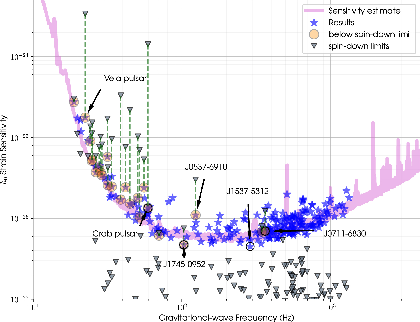
Figure 9: Upper limits on the GW strain, $h_{0}$, for 237 known pulsars obtained through targeted searches in the cumulative O1-O3 data of the LIGO and Virgo GW observatories [481]. Spin-down limits are shown as gray triangles, while blue stars highlight $95\%$ credible upper limits on $h_{0}$. Those pulsars where the GW information surpasses the spin-down limit are shown with orange circles. The pink curve represents the expected sensitivity of all three GW detectors during O3. Image reproduced with permission from [481]. Copyright by AAS.

As outlined in Sec. 3.3.3, rotating NSs with asymmetric deformations emit quasi-chromatic, continuous GWs. For small deformations and rigid rotation with angular frequency, $\Omega$, about a principle axis, a scenario typical for a NS with a mountain, the star loses energy according to Eq. (30) and emits GWs at $2\Omega$ with an amplitude given by Eq. (32). Corresponding NS observations constrain the ellipticity, $\varepsilon$.

First, because the GW luminosity can be at most equivalent to the loss of kinetic energy caused by the pulsar’s GW spin-down, pulsar timing data provide an upper limit on the ellipticity. The most stringent constraints on the maximum ellipticity that a NS can support come from young, energetic objects, because older NS are expected to retain little of their initial asymmetry unless they accrete matter from a companion (see below). For the Crab pulsar, we, for example, obtain the following spin-down limit from Eq. (31) assuming that the pulsar’s spin down is entirely driven by GW emission:

$$\varepsilon <7.4\times 10^{-4}\left(\frac{I_{3}}{10^{45}\,{\rm g}\,{\rm cm}^{2}}\right)^{-1/2}\left(\frac{P}{33\,{\rm ms}}\right)^{3/2}$$

$$\times\left(\frac{\dot{P}}{4.21\times 10^{-13}\,{\rm s}\,{\rm s}^{-1}}\right)^{1/2}.$$ (53)

For a pulsar with a radius of $R_{\rm NS}=10\,$km, this corresponds to a mountain height of $\sim\varepsilon R_{\rm NS}\lesssim 7.4\,$m.

Complementary constraints, beating the spin-down limits in several cases, come from the non-detection of continuous GW signals from NSs with advanced GW detectors (for recent reviews see [335, 326, 327]). These searches lead to upper limits on the maximum strain, $h_{0}$ (see Fig. 9), which in turn sets constraints on $\varepsilon$ via Eq. (32). Specifically

$$\varepsilon <2.4\times 10^{-5}\left(\frac{I_{3}}{10^{45}\,{\rm g}\,{\rm cm}^{2}}\right)^{-1}$$

$$\times\left(\frac{D}{1\,{\rm kpc}}\right)\left(\frac{P}{10\,{\rm ms}}\right)^{2}\left(\frac{h_{0}}{10^{-24}}\right).$$ (54)

For ‘blind’ all-Sky searches of unknown sources, current ellipticity limits span $\varepsilon\simeq 10^{-4}-10^{-5}$ [482, 483, 484]. Tighter constraints are obtained for studies of known or suspected pulsars, such as young NSs [485, 486, 481] (including those in supernova remnants [487, 488, 489]) or accreting compact objects in binaries [490, 491]. For example, for the Crab pulsar the spin-down limit (53) has been beaten by a factor $100$ [481]. The tightest upper limit on $\varepsilon$ comes from observations of an old MSP (PSR J0711–6830), which is $\varepsilon\lesssim 5.26\times 10^{-9}$ [481], corresponding to a mountain of less than $5.3\,$mm.

These constraints are important for several reasons. First, a number of physical mechanisms have been suggested as the cause for asymmetric deformations, but underlying physics are highly uncertain [e.g., 492, 493, 494]. This includes, e.g., intrinsic asymmetries due to non-axisymmetric magnetic-field configurations (so-called magnetic mountains [329, 495]), where we can estimate the ellipticity as

$$\varepsilon\simeq\frac{B^{2}R_{\rm NS}^{4}}{GM_{\rm NS}^{2}} \approx 1.9\times 10^{-12}\left(\frac{B}{10^{12}\,{\rm G}}\right)^{2}$$

$$\times\left(\frac{R_{\rm NS}}{10\,{\rm km}}\right)^{4}\left(\frac{M_{\rm NS}}{1.4M_{\odot}}\right)^{-2}.$$ (55)

This value falls well below current GW limits. Deformations might, however, be larger for young NSs with strong toroidal components and magnetars, where $\varepsilon$ can reach up to $10^{-6}$ [496, 497]. Another potential source of intrinsic asymmetry is the presence of superfluid and superconducting vortices in the stellar interior, which may lead to $\varepsilon\simeq 10^{-8}$ [330, 498, 499] (see also Sec. 3.8). However, relevant physics remain highly uncertain. Furthermore, accretion of matter from a companion star where composition gradients (strongly influenced by the magnetic-field configuration and accretion rate [496, 500, 501]) can lead to temperature asymmetries that cause thermal mountains [502, 503]. This effect covers a broad range of ellipticities $\varepsilon\simeq 10^{-11}-10^{-7}$ [501]. Observational GW constraints can thus provide insights into the underlying mechanisms driving the deformation.

Moreover, upper limits on $\varepsilon$ also link to the maximum ellipticity a NS can support [503, 504, 505, 506]. This directly connects to the highly uncertain dimensionless breaking strain, $\sigma$, of NS matter, which, e.g., determines crustal failure and associated multi-messenger phenomena outlined in Sec. 3.7.4. Assuming that the crust is maximally strained, [503] estimate that the largest ellipticity the NS crust can support is related to $\sigma$ as follows

$$\varepsilon \approx 1.6\times 10^{-6}\left(\frac{\sigma}{0.1}\right)\left(\frac{R_{\rm NS}}{10\,{\rm km}}\right)^{6.3}$$

$$\times\left(\frac{I_{\rm NS}}{10^{45}\,{\rm g}\,{\rm cm}^{2}}\right)^{-1}\left(\frac{M_{\rm NS}}{1.4M_{\odot}}\right)^{-1.2}.$$ (56)

While molecular dynamics simulations that model the crust as a Coulomb crystal suggest that the crust is very strong with $\sigma\sim 10^{-1}$ [507, 508], scaling these small-scale simulations to larger volumes remains uncertain. Observational GW constraints are, thus, valuable in determining independent information on $\sigma$ and assessing the crustal composition.

Note that the same considerations apply to deformations of possible crystalline phases of hybrid stars or solid quark stars [509, 510, 511, 512], which are generally able to support larger ellipticities than nucleonic NS crusts. For example, [513] recently discussed the sensitivity of crustal breaking on the nature of the phase transition between hadronic and quark matter in hybrid stars. Ellipticity limits, hence, also connect to the uncertain dense-matter EOS and the stellar core.

To summarize, continuous GW signals not only constrain crustal properties of NSs but can also provide information about the stellar magnetic field and the composition of matter in the NS core. However, as outlined above, while GW detections provide a direct upper limit on the stellar ellipticity and third-generation detectors have the potential to finally detect these continuous space-time disturbances [514], the processes generating NS mountains are still highly uncertain and degeneracies between the source distance and moment of inertia remain (see however Sec. 3.3.3), leading to the classification highlighted in Tab. 7.

3.7.4 Resonant shattering flares

As highlighted in Sec. 3.4, NSs in a binary system with a second NS or a low-mass BH are subject to tidal deformations close to the merger. In addition to the enhancement of GW emission, this effect could result in the shattering of the NS crust, which, in turn, may power EM emission before the merger, indirectly probing internal physics. This process has been proposed as an explanation for gamma-ray flashes, known as GRB precursors [515, 516, 517, 518], sometimes observed several seconds before short-duration GRBs. While a single tidal interaction is likely too weak to shatter the crust several seconds prior to merger, periodic tidal forces can enter into resonances with stellar oscillation modes during the inspiral phase [520, 521, 522]. [520] first identified the spheroidal $l=2$ $i$-mode as an ideal candidate for this resonance, which causes the mode to grow and releases energy into the crust. Once the stressed solid reaches its elastic limit (see Sec. 3.7.3), the crust shatters. The corresponding energy is transferred to the NS magnetic field, perturbing it in such a way as to generate an intense electric field that is able to accelerate the particles powering the gamma-ray flare. A necessary condition to attain the required acceleration is the presence of strong magnetic fields ($\gg 10^{13}\,\mathrm{G}$) at the surface of the NS [522]. This requirement prevents precursors to occur in all GRB events (in agreement with observations). We also note that confirming resonant shattering flares as origins of GRB precursors would imply the persistence of strong $B$-fields in old NSs, thus, setting constraints on the long-term evolution of the stellar magnetic field.

$i$-modes, or interface modes, originate from the presence of the interface between the liquid core and the solid crust. As a result, they are strongly influenced by the parameters describing the dense-matter EOS. In particular, $i$-modes are sensitive to the nuclear symmetry energy, which quantifies the change in binding energy per nucleon as the proton-neutron asymmetry increases. This dependence is noteworthy as macroscopic quantities, like the mass and radius, and characteristic frequencies of other quasi-normal modes like the $f$-mode, $p$-modes or $g$-modes (see Sec. 3.1.4), primarily depend on the EOS at the largest NS densities. As the composition in these regions is highly uncertain (and unlikely to be purely nucleonic), these observables provide only limited information about the nuclear symmetry energy. In contrast, at the crust-core interface, matter is purely nucleonic and resonant shattering excited by $i$-modes could, thus, probe this uncertain aspect of the EOS [524, 525]. However, to constrain the symmetry energy, detailed information about the mode frequency is necessary. This could be obtained by measuring the GW frequency of the chirp signal precisely at the moment when the resonant shattering flare occurs [524, 525]. The requirement of a simultaneous detection of GW and gamma-ray signals establishes this method as a truly multi-messenger technique.

Clearly, this method requires that short GRB precursors are powered by the mechanism outlined above. However, different mechanisms have been proposed to explain this phenomenon that do not involve the shattering of the NS crust (see, e.g., [526] for an alternative scenario that invokes intermittent accretion onto a newly born magnetar). A detection of the EM signal preceding a GW merger signal would, however, serve as confirmation of pre-merger models (like shattering flares models) for GRB precursors over models based on activity from the merger remnant. Moreover, even if powered by resonant crust shattering, different modes, such as the $f$-mode or $r$-modes might also be responsible for crustal failure [527] further complicating the comparison between data and theoretical models. Finally, we also point out that current models of crustal shattering typically neglect other pieces of physics that are likely relevant for the dynamics. This, e.g., includes the presence of nuclear pasta phases close to the crust-core interface (see Sec. 2.2), which would likely result in a frequency shift of the $i$-mode but leave its qualitative nature unaltered, or the possibility of plastic crustal flow [528, 529, 530]. The latter, if present, could significantly impact on the $i$-modes dynamics. For these reasons, we classify this method as strongly model dependent in Tab. 7.

3.7.5 Quasi-periodic oscillations in magnetar giant flares

QPOs are observed during giant flares in magnetars (see also Secs. 3.5.3 and 3.6.4). Based on theoretical calculations, these oscillations were initially thought to be connected with torsional shear modes of the stellar crust. In particular, the frequency of the fundamental mode can be estimated as [19]

$$f_{\rm s}\simeq\frac{v_{\rm s}}{2\pi R_{\rm NS}},$$ (57)

where $v_{\rm s}\equiv\sqrt{\mu_{\rm s}/\rho}$ is the crustal shear speed with $\mu_{\rm s}$ denoting the shear modulus. $\mu_{\rm s}$ is comparable to the Coulomb energy per unit volume of a crustal lattice site, thus introducing a significant dependence on crustal microphysics. Using an estimate from [458] for the shear modulus based on parameters from [531, 532], we deduce for the inner crust

$$f_{\rm s} \approx 17.4\left(\frac{\rho}{10^{14}\,{\rm g}\,{\rm cm}^{-3}}\right)^{1/6}\left(\frac{Z}{38}\right)\left(\frac{A}{302}\right)^{-2/3}$$

$$\times\left(\frac{1-X_{\rm n}}{0.25}\right)\left(\frac{R_{\rm NS}}{10\,{\rm km}}\right)^{-1}\,{\rm Hz}.$$ (58)

Here, $Z$ and $A$ denote the proton and total baryon number per lattice site, respectively, and $X_{\rm n}$ the fraction of neutrons that forms the free gas around the lattice nuclei (Sec. 2.2).

The value (58) is close to observed low-frequency QPOs. The association between measured frequencies and crustal shear modes, thus, provides constraints on dense matter. It, for example, allows us to probe the pasta phases at the base of the crust (see Fig. 2), since the shape of the pasta affects the solid’s elastic properties, i.e., the shear modulus, $\mu_{\rm s}$. In the case of cylindrical crustal nuclei, [533], e.g., finds a reduction in $\mu_{\rm s}$ and the shear mode frequency (see however [534]). Moreover, by identifying the $29\,$Hz QPO frequency in the 2004 giant flare of SGR 1806–20 [382] with the fundamental shear mode, [392, 535, 536] set constraints on the nuclear symmetry energy. Further EOS constraints have been obtained by modeling crustal shear modes in GR. As highlighted in Sec. 3.5.3, this introduces additional $R_{\rm NS}$ and $M_{\rm NS}$ dependencies, specifically connecting relevant mode frequencies with the radial extent of the NS crust, $\Delta R$, [390], which in turn is controlled by the EOS.

More recent studies have, however, shown that crustal vibrations are strongly damped as the $B$-field couples crust oscillations to the Alfvén continuum in the NS core [396, 398, 434] (see also Sec. 3.6.4). As a result, pure crustal shear modes are likely suppressed in magnetars, and replaced by combined magneto-elastic oscillations. Although these are similar in frequency to the shear modes outlined above, corresponding mode frequencies no longer depend on crustal properties only but also the stellar magnetic field. [406], for instance, find for the lowest-order low-frequency oscillation in the combined crust-core system (for a fixed EOS and NS mass):

$$f_{0} \simeq 2.8X_{\rm SF}^{-0.55}\left(\frac{v_{\rm s}}{1.37\times 10^{8}\,{\rm cm}\,{\rm s}^{-1}}\right)^{1/2}$$

$$+0.66X_{\rm SF}^{-0.33}\left(\frac{B}{10^{14}\,{\rm G}}\right)\,{\rm Hz},$$ (59)

where the parameter $X_{\rm SF}$ accounts for NS superfluidity (see Sec. 3.8.4 for details). Note that the numerical values here are obtained from fits to a specific set of simulations. Associating the observed high-frequency QPOs with magnetically modified crustal overtones as highlighted in Eq. (51) sets further combined constraints on the magnetic field and the crustal EOS. Connecting both expressions (59) and (51) with SGR 1806–20 observations, [406] use a Bayesian framework to deduce a relatively high shear speed of $v_{\rm s}\gtrsim 1.4\times 10^{8}\,{\rm cm}\,{\rm s}^{-1}$ and a large crustal thickness of $\Delta R\approx 1.61$ at $68\%$ credibility level together with $B\approx 2.1\times 10^{15}\,{\rm G}$ for the mean magnetic-field strength.

Although this approach holds promise to constrain highly uncertain crust physics, the crucial issue remains the correct identification of an observed mode frequency with the underlying oscillation mechanism. Moreover, crust and core physics are likely strongly coupled in magnetars, implying that crustal microphysics are difficult to disentangle from magnetic field properties. Combined with potential issues in extracting QPO properties from observations (Sec. 3.5.3), this leads us to classify this method as orange in Tab. 7.

3.7.6 Pulsar glitches

We introduced the glitch phenomenon in Sec. 3.3.2 in the context of moment-of-inertia measurements. However, in addition to probing macroscopic quantities, sudden spin-ups also provide information about the small-scale properties of the inner NS crust. This is due to the fact that glitches are intimately linked to the dynamics of superfluid vortices (see Sec. 3.8 for superfluid microphysics). These structures with diameters on the order of $100\,$fm exist since superfluids cannot rotate like classical fluids but instead quantize their circulation [537, 538]. Consequently, interactions of individual vortices and their environment are indirectly reflected in observed glitch properties, best measured in the radio band.

The key assumption for building up a superfluid angular momentum reservoir is that vortices can pin to the crustal lattice (and potentially also to superconducting proton fluxtubes in the NS core [e.g., 539, 540]), effectively impeding their motion and preventing the superfluid from spinning down on large scales. As the rest of the star slows down, the rotational lag between superfluid and normal matter grows, leading to a hydrodynamical lift force (the so-called Magnus force [e.g., 541, 542]) on small scales. Vortices unpin and move outwards once the lag is sufficiently large for the lift force to overcome the pinning threshold. Although the exact details of what follows are uncertain, this process drives an avalanche-like event unpinning millions of vortices in the inner crust. This allows the superfluid to spin down and exchange angular momentum with the crust, producing the glitch. The maximum pinning force between a vortex and a lattice site is, hence, closely connected to the size of the angular momentum reservoir and the maximum glitch a pulsar can exhibit [543, 312, 325]. Monitoring glitch statistics [544, 545], thus, informs theoretical calculations of relevant pinning forces, depending for example on the sizes of the crustal lattice nuclei and the vortices [e.g., 546, 547, 548, 549, 550]. Spin-up statistics are also an important tool to refine our understanding of the glitch trigger, which has been connected with, e.g., inhomogeneous vortex distributions [551] and superfluid instabilities [552, 553].

Once vortices are unpinned, frictional forces acting on the freed vortices and mechanisms governing their repinning control the post-glitch response on various timescales. Within hydrodynamical models, the coupling between different stellar components and, consequently the glitch morphology, are regulated by mutual friction, the coarse-grained dissipation between individual vortices and their environment [e.g., 541, 542]. Using a two-fluid approach has allowed the qualitative description of the full evolution of the Vela pulsar and other NSs showing giant glitches for realistic assumptions on the strength of mutual friction [312]. A three-component variant was recently proposed by [313] (see also [554]), specifically targeting the glitch rise on minute-long timescales. A comparison of this model with the first observation that caught a glitch in the act (the 2016 Vela pulsar glitch [298]) provided new information on internal coupling strengths [555], highlighting the potential of this approach in constraining the unknown properties of the NS crust (see also [556, 557, 558]).

Finally, observed post-glitch relaxation timescales on the order of weeks to months [e.g., 295, 296, 297, 299] have been used to estimate crustal temperatures within so-called vortex-creep models [e.g., 309, 559, 560, 561, 562]. Instead of focusing on mutual-friction forces as the driver for post-glitch dynamics, these models assume that superfluid vortices are imperfectly pinned and thermal activation allows a certain fraction to hop outwards to neighboring pinning sites as the star spins down. Following a glitch, the creep dynamics in the crust are altered, affecting the stellar spin-down rate and driving the observable relaxation. As these dynamics are sensitive to the temperature of the creep region, a comparison between the model and exponential relaxation timescales observed after Vela pulsar glitches has allowed rough constraints of the internal temperature [559]. Long-term relaxations are, however, not only accounted for within vortex-creep models. [563] recently showed that the post-glitch behavior of the Vela pulsar and PSR J0537–6910 can similarly be explained by the dynamics of a turbulent tangle of superfluid vortices. This highlights how sensitive current constraints on NS properties are to the underlying models.

In conclusion, while pulsar glitches are ultimately controlled by the interactions of individual vortices and their environments on small scales, thus indirectly probing the properties of the NS crust (and to a lesser extent those of the NS core [e.g., 539, 312, 562, 313, 558]), the glitch phenomenon encodes the dynamics of the entire star. Theoretical glitch models hence rely on averaging many orders of magnitude to bridge the gap between vortex scale and stellar scale. As a result, inferred parameters are strongly model dependent, leading to the classification shown in Tab. 7.

3.8 Superfluidity

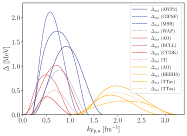
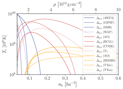
Figure 10: Superfluid energy gaps, $\Delta$, as a function of Fermi wave number, $k_{\rm F}$, (top panel) and the corresponding transition temperatures, $T_{\rm c}$, as a function of baryon density, $n_{\rm b}$, and mass-energy density, $\rho$, (bottom panel) for the three quantum phases in the NS interior. We illustrate a representative range of parameterized energy gaps with fit parameters from [564] (see this reference for more information on specific gaps shown in the legends): Curves for the singlet-paired neutrons in the NS crust are shown in blue (labeled n,s), gaps for the singlet-paired protons in the core in red (labeled p,s) and those for the triplet-paired core neutrons in orange (labeled n,t). Within BCS theory, the energy gap can be directly related to the transition temperature. In particular, in the zero-temperature limit, the two quantities are approximately related as $k_{\rm B}T_{\rm c}\approx 0.567\Delta$ for singlet pairing and $k_{\rm B}T_{\rm c}\approx 0.118\Delta$ for triplet pairing [564]. To show the density dependence of $T_{\rm c}$ throughout the NS core, we specifically considered the NRAPR EOS [565].

Method	GWs	Radio	Optical	X-ray	$\mathbf{\gamma}$-ray
Pulsar glitches
Cooling
Thermal post-outburst relaxation
Giant-flare QPOs

Table 8: Superfluidity measurements. Individual rows represent the methods that probe NS superfluidity, while columns denote different messengers/EM wavebands. Individual colors are equivalent to those in Tab. 1.

We previously highlighted the role of superfluid pulsar glitches when constraining the NS moment of inertia (Sec. 3.3.2) and properties of the stellar crust (Sec. 3.7.6). We now provide additional information on superfluid microphysics and relevant observational constraints thereof.

The suggestion that nucleons in NS interiors could form large-scale quantum condensates was put forward in [566] almost a decade before the first detection of radio pulsars [6]. While the properties of matter at such high densities remain uncertain, we suspect that NS older than a few hundred years are sufficiently cold [150, 148, 147, 40] for the neutrons in the inner crust and the neutrons and protons in the NS core to become unstable to the formation of Cooper pairs. This is analogous to electronic superconductors on Earth [567]. Generalizing the corresponding theory to NSs suggests that crustal neutrons and core protons experience pairing in a spin-singlet, $s$-wave state with vanishing angular momentum (${}^{1}S_{0}$), while the core neutrons pair in a spin-triplet, $p$-wave channel of non-zero angular momentum (${}^{3}P_{2}$) [e.g., 568]. The quantities of interest are the so-called pairing gaps, $\Delta$ (half the energy required to break a Cooper pair; see Fig. 10), which are directly related to the transition temperatures, $T_{\rm c}$, for the onset of superfluidity. These gaps control a number of astrophysically relevant properties of NSs (see [569] for a recent review). However, detailed calculations of pairing properties of superfluid neutrons and superconducting protons are difficult due to unknown many-body interactions and the importance of additional physics such as in-medium effects above saturation density [e.g., 570, 571, 572, 573, 574, 575, 576].

In this section, we, therefore, focus on those NS measurements that provide not only qualitative evidence for NS superfluidity but also give quantitative constraints on pairing and superfluid properties even if these are strongly model dependent (see Tab. 8).

3.8.1 Pulsar glitches

Superfluidity in the interior of NSs was initially invoked by [577] to explain the month-long relaxation timescales observed after the first Vela glitch [578, 579], its inviscid nature providing a natural justification for weak internal interactions manifest in the long-term relaxation. This notion gained further credence with laboratory experiments using superfluid helium demonstrating similar behavior [580].

As discussed in Sec. 3.7.6, glitch dynamics are ultimately controlled by the physics of individual vortices and, hence, sensitive to pairing properties. In the standard theory for laboratory superconductors [567], the diameter of a vortex corresponds to the coherence length, $\xi$, of the superfluid condensate and is, therefore, connected to the energy gap as

$$\xi=\frac{\hbar v_{\rm F}}{\pi\Delta} \approx 1.2\times 10^{-12}\left(\frac{\Delta}{1\,{\rm MeV}}\right)^{-1}$$

$$\times\left(\frac{v_{\rm F}}{6\times 10^{-9}\,{\rm cm}\,{\rm s}^{-1}}\right)\,{\rm cm},$$ (60)

where $v_{\rm F}$ is the Fermi velocity. However, measured glitch parameters are typically insensitive to details of the underlying microphysics. Instead, spin-up models invoke the existence of internal superfluids to motivate a multi-component description as outlined in Sec. 3.3.2. In this coarse-grained framework, small-scale dynamics are averaged out in favor of a model for the entire star, resulting in the loss of information of pairing physics.

As a result, pulsar glitches present strong qualitative evidence for the existence of NS superfluidity but current measurements and models are insufficient to provide quantitative constraints on microscopic superfluid properties. We, therefore, classify this method as orange in Tab. 8.

3.8.2 Cooling of isolated neutron stars

Additional constraints on superfluid pairing can be obtained by observing the cooling of isolated NSs, whose thermal radiation from their surfaces is observable in the X-rays [e.g., 148, 147, 581]. As discussed in Sec. 3.1.5, the emission of neutrinos from the stellar interior dominates the cooling of NSs younger than $\sim 100\,{\rm kyr}$, while photon emission from the surface plays a crucial role at later times. Extracting temperatures from the X-ray emission of young objects [377, 582, 40, 31], thus, has the potential to provide insights into the composition of the cooling matter.

The young ($\approx 330\,{\rm yr}$ old) CCO in the supernova remnant Cassiopeia A has been of particular interest in this context, because its surface temperature appears to decrease faster than expected within the standard neutrino cooling scenario [583, 584], which invokes modified Urca processes [150, 148, 147, 40]. Although, the effect is difficult to detect and requires detailed understanding of telescope systematics and emission processes [585, 586], its presence hints at unmodeled physics. While a number of interpretations have been put forward [e.g., 587, 588, 589, 590], such an anomalous temperature drop can be explained naturally by the recent onset of large-scale superfluidity [591, 592]. While the presence of superfluidity suppresses Urca reactions, it also reduces the matter’s heat capacities and results in additional neutrino emission due to the continuous breaking and forming of Cooper pairs close to the superfluid transition temperature. The net effect is faster cooling compared to the scenario without macroscopic quantum phases. Specifically, the size of the observed Cassiopeia A temperature drop allowed a constraint of the maximum critical temperature of the core neutrons to $\sim 5-10\times 10^{8}\,{\rm K}$, while also requiring the protons to already be superconducting, i.e., have an even higher $T_{\rm c,max}$ [591, 592, 593, 594]. Applying the same modeling approach to other young NSs at the centers of supernova remnants (notably the compact object hypothesized to have formed in the Galactic supernova SN 1987A) leads to broadly consistent results [595, 596].

In summary, closely monitoring the cooling behavior of young, isolated NSs gives quantitative information about the onset of superfluidity in NSs, provided that the temperature drop is indeed real and caused by a superfluid transition. This approach, hence, allows us to constrain uncertain energy gaps. However, systematics in extracting accurate temperature measurements currently hinder tighter gap constraints, leading us classify this method as orange in Tab. 8.

3.8.3 Thermal relaxation of quasi-persistent X-ray transients

The concepts underlying thermonuclear X-ray bursts were discussed in detail in Secs. 3.2.2 and 3.7.2. Monitoring the quiescent emission of those systems that undergo outbursts after extended periods of accretion (quasi-persistent transients) are of particular interest in the context of extracting superfluid parameters.

In particular, if the neutrons in the inner crust are superfluid, their heat capacity is significantly suppressed (as it is the case in isolated NS; see Sec. 3.8.2), resulting in faster cooling. In contrast, in those layers where neutrons are normal (non-superfluid), they constitute the dominant contribution to the heat capacity, store more heat and, therefore, delay the thermal relaxation. The shape of the cooling curves of quasi-persistent transients on intermediate timescales is thus sensitive to the nature of the crustal neutrons and observations of enhanced cooling in this intermediate regime suggest that crustal superfluidity is indeed present [e.g., 475, 472]. In particular, cooling curves are dependent on ‘how many’ of the crustal neutrons are superfluid, which in turn probes the shape of the pairing gap. As illustrated in the bottom panel of Fig. 10, it is unknown at which densities the singlet-pairing gap closes (i.e., when $T_{\rm c}$ drops to zero) and whether it does so before the crust-core boundary located at $\sim 10^{14}{\,\rm g\,cm}^{-3}$ or at higher densities in the core. If the former is the case, this would imply the presence of a normal layer of neutrons between the crustal and the core superfluids, effectively delaying the cooling. [478] indeed found evidence for such a late-time thermal relaxation.

Though quasi-persistent transients become increasingly faint and thus difficult to detect, sensitive X-ray telescopes have observed the cooling behavior of a few objects several years post outbursts [e.g., 597, 598]. Such measurements hold particular promise: the longer we observe the thermal relaxation, the deeper we probe into the stellar interior, i.e., the cooling curve on long timescales is sensitive to NS core physics. This is especially powerful if the outburst itself and the subsequent cooling are monitored, as this allows an estimate of the energy deposited into the core and constraints on the NS envelope composition, a major model uncertainty. Combined with temperature and neutrino-luminosity estimates, we can therefore get a handle on the core’s heat capacity, which in turn sets constraints on the properties of dense matter. While [597] used this approach to rule out NS cores dominated by a quark color-flavor-locked phase in several systems, [598] were able to show that observations of another source are difficult to reconcile with a significant presence of core superfluidity and superconductivity.

In conclusion, although models are complex and several systematics, such as the NS envelope compositions and distances, often difficult to assess (leading to the classification in Tab. 8), long-term thermal relaxations of NSs that show outbursts after years to decades of accretion provide a unique view into the stellar interior. In particular, monitoring the cooling curve with time allows us to look deeper and deeper into the star providing unique quantitative constraints on the matter’s pairing properties.

3.8.4 Quasi-periodic oscillations in magnetar giant flares

Superfluidity has a significant impact on the NS oscillation spectrum [e.g., 599, 45]. Magnetar QPOs, hence, also encode information about macroscopic quantum phases in NS interiors. In particular, superfluidity plays a crucial role in explaining observations of high-frequency QPOs [380], which are difficult to explain with the physical mechanisms explained in Secs. 3.5.3, 3.6.4 and 3.7.5 alone. Although the crust can, in principle, vibrate at frequencies of several hundred Hz, these oscillations should be strongly damped due to coupling to the core, making it difficult to reconcile observations of long-lasting high-frequency QPOs (see however [600] for a discussion of potential detection biases).

Treating the core superfluid in an effective manner, [401, 402] find that magneto-elastic models with superfluidity can produce oscillations at high frequencies. As a result of superfluidity, core neutrons and protons are coupled, involving a larger fraction of mass in the stellar oscillations. [403, 406] encapsulate this interaction in an effective parameter $X_{\rm sf}\equiv\epsilon_{\star}X_{\rm p}$, where $\epsilon_{\star}$ measures the coupling between the neutrons and protons via the entrainment effect (see, e.g., [541, 542]) and $X_{\rm p}$ denotes the fraction of protons. In this picture, the mechanism responsible for generating a giant flare excites initial crustal modes, which subsequently resonantly excite a few specific torsional Alfvén overtones in the core. This could explains why only a few high-frequency modes are observed and not the full spectrum excited. Moreover, the range of possible high-frequency QPOs decreases for increasing $X_{\rm sf}$ [406], highlighting that observations of these modes put constraints on superfluid properties.

This is particularly powerful in combination with the impact of superfluidity on the low-frequency magneto-elastic modes, discussed in Sec. 3.7.5. Specifically, the parameter $X_{\rm sf}$ also affects the frequency of the fundamental oscillation as given in Eq. (59), obtained from fits to numerical simulations. Combining low- and high-frequency QPOs from SGR 1806–20 [380], [406] obtain $X_{\rm sf}\approx 0.09$ at $68\%$ confidence level. This value is close to $0.046$ which is representative of a fully superfluid model [531] and, thus, hints at a significant fraction of the NS star being in a superfluid state.

In addition to the uncertainties around accurately identifying oscillation physics with measured QPOs frequencies, degeneracies between model parameters and observational biases (see Secs. 3.5.3, 3.6.4 and 3.7.5), current models of superfluid magneto-elastic oscillations neglect a number of relevant physics. The effective prescription based on the parameter $X_{\rm sf}$ introduced above describes the star as a single fluid, neglecting the multi-component nature of NS interiors. Moreover, the influence of superfluid vortices as well as the presence of superconductivity have been ignored to date. Advanced simulations that incorporate a more realistic treatment of superfluids in magneto-elastic media (e.g., based on [601, 602]) will be needed to drive this approach forward. As a result of these caveats, we classified this method as strongly model dependent in Tab. 8.

3.9 Further multi-messenger measurements

To conclude, we focus on a few additional approaches that provide insights into NS characteristics but which did not fit with our categories presented in the previous sections. In particular, multi-messenger astrophysics provides the opportunity to study a single celestial source with different messengers, including photons, GWs, and neutrinos. The advantage of employing multiple messengers is that they offer complementary information, providing unique insights into the source’s properties, as exemplified in Sec. 3.2.4. In this section, we briefly outline two additional angles for deducing NS properties from multi-messenger observations.

3.9.1 Kilonovae

The advent of the multi-messenger era offers us several other ways to study NSs through the different EM transients associated with BNS and NS-BH mergers. For recent reviews of EM counterparts to GW signals, we refer the reader to [247, 248]. In particular, during a CBM, a fraction of the NS’s matter, typically $<0.1\,M_{\odot}$ [e.g., 603], can be ejected and become gravitationally unbound from the system. This matter, heated by internal radioactive decay, powers the transient optical and near-infrared CBM counterpart known as KN [604, 605, 606, 607, 608] (see [609] for a comprehensive review of theoretical and observational aspects).

The ejection of matter can occur through different channels like tidal forces, shocks at the interface between the two stars (for a BNS merger), or accretion disk winds. These ejecta components are characterized by different masses, velocities, and chemical compositions, and consequently different opacities, which determine the observational properties of KNe, such as their peak luminosity, temperature, and time at which the emission peaks. As these observable parameters, and the relative importance of the different ejecta components, are influenced by characteristics of the binary system, such as its total mass, the components’ mass ratio and the NS EOS, observations of KNe, thus, encode information on the properties of dense matter [609].

Moreover, the nature of the merger remnant is affected by the EOS and impacts on the KN. In particular, whether the merger leads to the prompt formation of a BH, the formation of a metastable NS that subsequently experiences delayed collapse into a BH, or the formation of a stable NS, depends not only on the two binary masses but also on the dense-matter EOS. For example, stiffer EOSs produce longer-lived (and eventually stable) NS remnants, while softer EOSs are associated with prompt collapse to a BH [e.g., 610, 611].

If the remnant is indeed a metastable or stable NS rather than a BH, emitted neutrinos irradiate the ejecta matter, which increases its proton fraction and prevents the production of lanthanides. Without these lanthanides, which are characterized by high opacities, the KN would be bluer in color and evolve faster [612, 613]. Moreover, the presence of a NS remnant is also expected to lead to an increase of ejected matter because additional material can be ablated from the stellar surface due to neutrino irradiation [614, 615, 616, 617, 618] or the magnetic pressure from the interior of the NS remnant [619, 620]. This additional matter-ejection channel enhances the blue component of the KN emission at early times (i.e., within $\sim 1\,{\rm day}$ after the merger) [621]. To assess the presence of a NS remnant, observing the transient at early times is thus crucial. To this aim, GWs can act as a trigger to guide optical follow-up observations and help catch the first phase of this transient.

We note that multi-messenger observations of GW170817 have already been exploited to constrain NS parameters. For example, [622] combined limits on the ejecta mass from observations of the GRB and KN following the merger with the system’s total mass inferred from the GW signal to obtain a limit on the maximum mass of a NS. They find $M_{\rm max}=2.17\,M_{\odot}$ at $90\%$ confidence level. The idea is that, for a given total mass of the binary, the remnant would have undergone prompt collapse into a BH if the maximum mass is not sufficiently large. Such a prompt collapse is inconsistent with the large fraction of lanthanide-free ejecta observed from the KN. On the other hand, if the maximum mass is too high, the collapse is sufficiently delayed for the remnant to inject its rotational energy through magnetic dipole emission (see Sec. 3.6.1) into the ejecta and/or the GRB jet, which is also inconsistent with observations. Interestingly, the above constraint is similar to the mass limit of $M_{\rm max}=2.16\,M_{\odot}$ obtained by [277] from the GW signal along, i.e., without relying on modeling the EM counterpart.

Finally, the EOS also affects the so-called KN-afterglow, which is an emission powered by the shock of the ejecta onto the interstellar medium [624, 625, 626, 627]. The properties of this emission, such as the peak flux and peak time, are greatly influenced by the presence and the characteristics of the fast ($\gtrsim 0.7\,c$), mildly-relativistic component of the CBM ejecta. This ejecta component, in turn, is launched by shocks induced either by remnant oscillations or at the contact interface between the two merging NSs [625, 628]. Both mechanisms are dependent on the NS EOS, with softer relations associated with faster ejecta [626, 627], thus, resulting in EOS-sensitive KN-afterglows.

To summarize, the study of EM transients that accompany CBMs allows us to probe the unknown EOS of NSs. Future CBMs multi-messenger observations will be crucial to fully explore the potential of this approach, which to date has been limited by the small number of observed events. In the spirit of previous sections, we, however, point out that KNe are complex and corresponding frameworks strongly model dependent, i.e., many individual ingredients influence their observable features, complicating EOS constraints.

3.9.2 Neutrinos

As a final remark, we note that while we have touched upon the indirect impact of neutrinos on NS properties (see Secs. 3.1.5, 3.7.2, 3.8.2, 3.8.3), we have neglected their role as direct messengers for constraining NS physics. In particular, we remind the reader that neutrinos are crucial for the secular evolution of NSs, because they drive NS cooling during the first $\sim\mathcal{O}(10\,\mathrm{kyr})$ of the star’s life (see [150, 147] for detailed reviews). As different processes are involved in this secular cooling, the ability to distinguish between them would allow us to gain insights into the stellar composition and the onset of superfluidity (see Sec. 3.8). However, direct detection of these neutrinos is not possible with present and future facilities, because on one hand neutrino energies (which are of the order of the NS temperature, i.e., $<1\,\rm MeV$) are too low to be detected, and on the other they are likely too low in flux (see [150] for typical neutrino emissivities). Instead, the best way to constrain these processes is indirectly, through the observation of thermal emission in the EM wavebands as described in previous sections.

Neutrinos are also emitted during violent events involving NSs such as BNS mergers. Whereas thermal neutrinos are difficult to detect [629], the neutrinos produced by non-thermal merger processes may be detectable by facilities like IceCube or KM3net, even though to date no such neutrinos have been observed [630]. However, the origins of these non-thermal neutrinos are most likely connected to the acceleration of hadrons in shocks occurring in relativistic outflows. Although of interest for constraining the physics of particle acceleration and the outflow’s composition, we do not expect these neutrinos to directly probe the physics of NSs.

In the NS context, the most interesting sources for the emission of detectable neutrinos are core-collapse supernovae. Supernova SN1897A in the Large Magellanic Cloud, which was detected via its EM and neutrino emission [631, 632], was the first astrophysical transient accessible with multiple messengers. Such a supernova neutrino signal can provide us with information about the explosion mechanism, and the resulting proto-NS. However, covering this topic was beyond the scope of this review and we instead refer the interested reader to [633] and references therein.

4 Summary and Conclusions

The study of NSs presents fascinating opportunities for scientific exploration. These compact objects, characterized by strong gravity, high densities, large magnetic fields and fast rotation, offer insights into the properties of matter and strong interactions under extreme conditions that we cannot replicate in terrestrial environments. However, as we demonstrated in this review, measuring the characteristics of NSs and using these to constrain dense-matter physics is a challenging task. We specifically outlined techniques and underlying model assumptions and systematics used to extract global observables, focusing on the NS mass (Sec. 3.1), radius (Sec. 3.2), moment of inertia (Sec. 3.3), tidal deformability (Sec. 3.4), and compactness (Sec. 3.5). This was followed by a discussion of measuring non-global quantities, specifically the NS magnetic field (Sec. 3.6), crustal physics (Sec. 3.7) and superfluidity (Sec. 3.8).

To overcome individual measurement challenges and advance our understanding of NSs, the development of independent methods targeting different observables and relying on distinct assumptions is crucial. This approach allows for cross-validation and reduces the reliance on specific models. The exploration of different NS classes and associated phenomena (Sec. 2.1) using a multi-wavelength and multi-messenger approach, which involves complementary information from observations across the EM spectrum as well as the GW domain, is particularly useful in forming a more comprehensive view of these objects.

Among the methods discussed, radio timing of pulsars in binary systems stands out. These observations have proven particularly effective in constraining NS masses, and might also provide moment-of-inertia measurements in the future. This technique, which leverages the incredible stability of radio pulsar signals, offers several advantages, including high precision and reduced model dependence, compared to other methods discussed. Note that monitoring how young, isolated pulsars divert from their stable behavior and analyzing these glitches in details, provides further information on internal physics. However, underlying model uncertainties currently limit us to using these irregularities primarily for qualitative constraints. With the Square Kilometre Array (expected to detect all visible Galactic radio pulsars and to monitor them with unprecedented precision) having finally begun construction in 2022, we expect radio timing to continue to play an essential role in determining NS parameters.

We further highlighted that the NS radius is the macroscopic quantities that is the hardest to measure. Many of the methods we presented suffer from strong model dependencies. However, we concluded that the most promising and least model-dependent approach is to measure the radius through X-ray pulse-profile modeling of MSPs. By analyzing thermal emission patterns on the surfaces of these rapidly rotating NSs, valuable insights into their sizes can be gained. Monitoring the X-ray emission of other NS classes, such as accreting NSs after outbursts or young isolated CCOs, to track their thermal evolution, provides complementary information on the stellar interior, although significant uncertainties remain due to the complexity of modeling internal NS physics. The same holds for decoding observations of strongly magnetized magnetars after giant flares or individual emission features. Future X-ray missions, such as ATHENA, will expand the sensitivity limits of existing observatories and allow us to provide better radius constraints and look deeper into the NS crust and core.

In addition to EM observations, the recent detections of BNS and NS-BH mergers in the GW band have opened up an entirely new avenue to study NSs. GWs have specifically enabled new measurements of NS masses and first constraints on the tidal deformability. Further dense-matter constraints (although prone to strong uncertainties) have been possible due to the observations of EM merger counterparts including short GRBs and KNe. In the future, the increased sensitivity of next-generation GW interferometers, such as the Einstein Telescope and Cosmic Explorer, holds great promise for further enhancing our understanding of NS physics. Achieving higher sensitivity will allow for the detection of more distant signals, significantly increasing the number of detected merger events. This will enable more precise tidal-deformability and mass measurements, complemented by ongoing multi-messenger efforts. Advanced instruments will also finally enable the analysis of currently unexplored aspects of NS physics, such as the emission of continuous GWs, and allow us to take full advantage of asteroseismology to measure global and non-global properties of NSs.

In summary, studying NSs is a complex and challenging endeavor that offers remarkable opportunities for scientific advancement. By employing a variety of measurement techniques, embracing a multi-wavelength approach, and taking advantage of GW astronomy, we can deepen our understanding of these intriguing objects. The development of new observational capabilities, combined with a push for better theoretical models, holds great promise for shedding light on the (as yet unknown) physics of these extreme stars.

Author contributions

S. A. and V. G. contributed equally to this work.

Acronyms and variable definitions

We have defined the following acronyms in this work:

BH	Black Hole
BNS	Binary Neutron Star
CBM	Compact Binary Merger
CCO	Central Compact Object
CFS	Chandrasekhar-Friedman-Schutz
CRSF	Cyclotron Resonance Scattering Feature
EM	Electromagnetic
EOS	Equation of State
GR	General Relativity
GRB	Gamma-Ray Burst
GW	Gravitational Wave
HMXB	High-Mass X-ray Binary
ISCO	Innermost Stable Circular Orbit
KN	Kilonova
LMXB	Low-Mass X-ray Binary
LOS	Line of Sight
MSP	Millisecond Pulsar
NICER	Neutron Star Interior-Composition Explorer
NS	Neutron Star
PN	Post-Newtonian
PRE	Photospheric Radius Expansion
QPO	Quasi-Periodic Oscillation
RRAT	Rotating Radio Transient
SNR	Signal-to-Noise Ratio
SuNR	Supernova Remnant
WD	White Dwarf
XDINS	X-ray Dim Isolated Neutron Star

We further defined the following variables in the review:

$\rho_{0}$	nuclear saturation density
$P$	NS spin period
$\dot{P}$	time derivative of NS spin period
$\tau_{c}$	NS characteristic age
$B_{\mathrm{dip}}$	NS surface dipolar magnetic field strength
$E_{\mathrm{rot}}$	NS rotational energy
$L_{\mathrm{rot}}$	NS rotational luminosity ($|\dot{E}_{\mathrm{rot}}|$)
$I_{\mathrm{NS}}$	NS moment of inertia
$T_{\mathrm{BB}}$	black-body temperature
$\rho_{\mathrm{NS}}$	neutron drip density
$M_{\mathrm{NS}}$	NS (gravitational) mass
$f_{\mathrm{bin}}$	binary system mass function
$M_{\mathrm{c}}$	mass of the binary companion
$i$	binary system inclination angle
$K_{\mathrm{c}}$	radial velocity of the binary companion
$P_{\mathrm{orb}}$	binary system orbital period
$e$	binary system eccentricity
$K_{\mathrm{NS}}$	NS radial velocity
$a$	binary orbital separation
$\dot{\omega}$	periastron advance
$\dot{P}_{\mathrm{orb}}$	rate of orbital decay
$\gamma$	Einstein delay
$M$	total mass of the binary system
$r$	Shapiro delay range
$s$	Shapiro delay shape
$a_{1}$	semi-major axis of the orbit
$x$	projected semi-major axis
$f_{\mathrm{GW}}$	GW frequency
$\dot{f}_{\mathrm{GW}}$	GW frequency time derivative
$\mathcal{M}$	chirp mass
$\omega_{f,w,r}$	($f,w,r$)-mode frequency
$\tau_{f,w}$	($f,w$)-mode damping time
$T$	temperature
$C_{v}$	heat capacity
$f_{\mathrm{amp}}$	amplified flux
$R_{\mathrm{e}}$	Einstein ring radius
$R_{\mathrm{NS}}$	NS radius
$R_{\infty}$	NS apparent radius
$D$	source distance
$F_{\infty}$	bolometric flux
$C_{\mathrm{NS}}$	NS compactness
$F_{\mathrm{Edd}}$	Eddington flux
$L_{\mathrm{Edd}}$	Eddington luminosity
$X_{\rm e}$	electron fraction
$T_{\mathrm{col}}$	color temperature
$g_{\mathrm{eff}}$	effective surface gravity
$A_{\infty}$	apparent area
$f_{\mathrm{c}}$	color factor
$N_{H}$	hydrogen column density
$E_{\mathrm{GRB}}$	GRB energy
$M_{\mathrm{disk}}$	accretion disk mass
$a_{\mathrm{BH}}$	dimensionless BH spin parameter
$\epsilon_{\mathrm{jet}}$	jet-launching efficiency
$M_{\mathrm{BH}}$	BH mass
$\mathbf{S}$	spin angular momentum
$\mathbf{L}$	orbital angular momentum
$P_{\mathrm{precession}}$	precession period
$\Omega$	angular velocity
$I_{\mathrm{sf}}$	superfluid moment of inertia
$\omega_{\mathrm{c}}$	critical angular velocity lag
$t_{\mathrm{glitch}}$	inter-glitch time
$\langle\mathcal{A}\rangle$	average glitch activity parameter
$I_{3}$	moment of inertia along rotation axis
$\epsilon$	NS ellipticity
$h_{0}$	GW amplitude
$n$	braking index
$\mathcal{E}_{i,j}$	tidal field
${Q}_{i,j}$	quadrupole moment
$\lambda_{\mathrm{NS,c}}$	tidal deformability
$k_{2}$	$l=2$ tidal love number
$\tilde{\Lambda}$	binary’s tidal deformability parameter
$\Lambda_{\mathrm{NS,c}}$	dimensionless tidal deformability
$\chi$	dimensionless spin parameter
$z$	gravitational redshift
$f$	QPO frequency during giant flare
$\psi$	angle between magnetic and rotation axis
$E_{\mathrm{cyc}}$	energy of cyclotron line
$n_{L}$	Landau level number
$B$	magnetic field strength
$f_{\mathrm{A}}$	frequency of Alfvén oscillation
$v_{\mathrm{A}}$	Alfvén velocity
$\rho_{\mathrm{c}}$	(mass) density of charged particles
$f_{\mathrm{crust}}$	frequency of crustal oscillations
$L_{\mathrm{neutrino}}$	neutrino luminosity
$L_{\mathrm{photon}}$	photon luminosity
$L_{\mathrm{crustal\,heating}}$	heat generated in X-ray bursts
$Q$	heating per accreted nucleon
$\langle\dot{M}\rangle$	time-averaged accretion rate
$f_{\mathrm{s}}$	frequency of torsional shear mode
$v_{\mathrm{s}}$	crustal shear speed
$\mu_{\mathrm{s}}$	shear modulus
$\rho$	mass density
$Z$	atomic number
$A$	mass number
$X_{\mathrm{n}}$	neutron fraction
$\xi$	superfluid coherence length
$v_{F}$	Fermi velocity
$\Delta$	pairing energy gap
$T_{\mathrm{c}}$	critical temperature for superfluidity
$k_{\mathrm{F}}$	Fermi wave number
$n_{\mathrm{b}}$	baryon number density
$\epsilon_{\star}$	entrainment parameter
$X_{\mathrm{p}}$	proton fraction
$M_{\mathrm{max}}$	maximum mass of a NS

References

- Abbott et al. [2017a] B. P. Abbott, et al., Physical Review Letters 119 (2017a) 161101. doi:10.1103/PhysRevLett.119.161101. arXiv:1710.05832.
- Abbott et al. [2017b] B. P. Abbott, et al., Astrophysical Journal Letters 848 (2017b) L12. doi:10.3847/2041-8213/aa91c9. arXiv:1710.05833.
- Landau [1932] L. D. Landau, Physikalische Zeitschrift der Sowjetunion 1 (1932) 285.
- Yakovlev et al. [2013] D. G. Yakovlev, et al., Physics Uspekhi 56 (2013) 289--295. doi:10.3367/UFNe.0183.201303f.0307. arXiv:1210.0682.
- Baade and Zwicky [1934] W. Baade, F. Zwicky, Physical Review 46 (1934) 76--77. doi:10.1103/PhysRev.46.76.2.
- Hewish et al. [1968] A. Hewish, et al., Nature 217 (1968) 709--713. doi:10.1038/217709a0.
- Kaspi and Kramer [2016] V. M. Kaspi, M. Kramer, arXiv e-prints (2016) arXiv:1602.07738. doi:10.48550/arXiv.1602.07738. arXiv:1602.07738.
- Keane and Kramer [2008] E. F. Keane, M. Kramer, Monthly Notices of the Royal Astronomical Society 391 (2008) 2009--2016. doi:10.1111/j.1365-2966.2008.14045.x. arXiv:0810.1512.
- Kaspi [2010] V. M. Kaspi, Proceedings of the National Academy of Science 107 (2010) 7147--7152. doi:10.1073/pnas.1000812107. arXiv:1005.0876.
- Viganò et al. [2013] D. Viganò, et al., Monthly Notices of the Royal Astronomical Society 434 (2013) 123--141. doi:10.1093/mnras/stt1008. arXiv:1306.2156.
- Popov [2023] S. B. Popov, Universe 9 (2023) 273. doi:10.3390/universe9060273. arXiv:2306.02084.
- Lorimer and Kramer [2012] D. R. Lorimer, M. Kramer, Handbook of Pulsar Astronomy, 2012.
- Goldreich and Julian [1969] P. Goldreich, W. H. Julian, Astrophysical Journal 157 (1969) 869. doi:10.1086/150119.
- Ruderman and Sutherland [1975] M. A. Ruderman, P. G. Sutherland, Astrophysical Journal 196 (1975) 51--72. doi:10.1086/153393.
- Graber et al. [2023] V. Graber, et al., arXiv e-prints (2023) arXiv:2312.14848. doi:10.48550/arXiv.2312.14848. arXiv:2312.14848.
- McLaughlin et al. [2006] M. A. McLaughlin, et al., Nature 439 (2006) 817--820. doi:10.1038/nature04440. arXiv:astro-ph/0511587.
- Keane et al. [2011] E. F. Keane, et al., Monthly Notices of the Royal Astronomical Society 415 (2011) 3065--3080. doi:10.1111/j.1365-2966.2011.18917.x. arXiv:1104.2727.
- Lewis and McLaughlin [8 24] E. Lewis, M. McLaughlin, RRAT Catalogue, https://github.com/rratalog/rratalog, Accessed: 2023-08-24.
- Turolla et al. [2015] R. Turolla, et al., Reports on Progress in Physics 78 (2015) 116901. doi:10.1088/0034-4885/78/11/116901. arXiv:1507.02924.
- Kaspi and Beloborodov [2017] V. M. Kaspi, A. M. Beloborodov, Annual Review of Astronomy and Astrophysics 55 (2017) 261--301. doi:10.1146/annurev-astro-081915-023329. arXiv:1703.00068.
- Rea and Esposito [2011] N. Rea, P. Esposito, in: High-Energy Emission from Pulsars and their Systems, volume 21 of Astrophysics and Space Science Proceedings, p. 247. doi:10.1007/978-3-642-17251-9_21. arXiv:1101.4472.
- Duncan and Thompson [1992] R. C. Duncan, C. Thompson, Astrophysical Journal Letters 392 (1992) L9. doi:10.1086/186413.
- Thompson and Duncan [1993] C. Thompson, R. C. Duncan, Astrophysical Journal 408 (1993) 194. doi:10.1086/172580.
- Thompson et al. [2002] C. Thompson, et al., Astrophysical Journal 574 (2002) 332--355. doi:10.1086/340586. arXiv:astro-ph/0110677.
- Haberl [2007] F. Haberl, Astrophysics and Space Science 308 (2007) 181--190. doi:10.1007/s10509-007-9342-x. arXiv:astro-ph/0609066.
- Turolla [2009] R. Turolla, in: W. Becker (Ed.), Astrophysics and Space Science Library, volume 357 of Astrophysics and Space Science Library, p. 141. doi:10.1007/978-3-540-76965-1_7.
- Manchester et al. [2005] R. N. Manchester, et al., Astronomical Journal 129 (2005) 1993--2006. doi:10.1086/428488. arXiv:astro-ph/0412641.
- Australia Telescope National Facility [8 24] Australia Telescope National Facility, ATNF Catalogue, https://www.atnf.csiro.au/research/pulsar/psrcat/, Accessed: 2023-08-24.
- Olausen and Kaspi [2014] S. A. Olausen, V. M. Kaspi, Astrophysical Journal Supplement 212 (2014) 6. doi:10.1088/0067-0049/212/1/6. arXiv:1309.4167.
- Olausen and Kaspi [0 23] S. A. Olausen, V. M. Kaspi, McGill Online Magnetar Catalogue, https://www.physics.mcgill.ca/~pulsar/magnetar/main.html, Accessed: 2023-10-23.
- Coti Zelati et al. [2018] F. Coti Zelati, et al., Monthly Notices of the Royal Astronomical Society 474 (2018) 961--1017. doi:10.1093/mnras/stx2679. arXiv:1710.04671.
- Coti Zelati et al. [0 23] F. Coti Zelati, et al., Magnetar Outburst Online Catalogue, http://magnetars.ice.csic.es, Accessed: 2023-10-23.
- Pavlov et al. [2004] G. G. Pavlov, et al., in: F. Camilo, B. M. Gaensler (Eds.), Young Neutron Stars and Their Environments, volume 218, p. 239. doi:10.48550/arXiv.astro-ph/0311526. arXiv:astro-ph/0311526.
- de Luca [2008] A. de Luca, in: C. Bassa, et al. (Eds.), 40 Years of Pulsars: Millisecond Pulsars, Magnetars and More, volume 983 of American Institute of Physics Conference Series, pp. 311--319. doi:10.1063/1.2900173. arXiv:0712.2209.
- Viganò and Pons [2012] D. Viganò, J. A. Pons, Monthly Notices of the Royal Astronomical Society 425 (2012) 2487--2492. doi:10.1111/j.1365-2966.2012.21679.x. arXiv:1206.2014.
- Giacconi [1974] R. Giacconi, in: C. Dewitt-Morette (Ed.), Gravitational Radiation and Gravitational Collapse, volume 64, p. 147.
- Done et al. [2007] C. Done, et al., Astronomy and Astrophysics Review 15 (2007) 1--66. doi:10.1007/s00159-007-0006-1. arXiv:0708.0148.
- Fornasini et al. [2023] F. M. Fornasini, et al., arXiv e-prints (2023) arXiv:2308.02645. doi:10.48550/arXiv.2308.02645. arXiv:2308.02645.
- Avakyan et al. [2023] A. Avakyan, et al., Astronomy and Astrophysics 675 (2023) A199. doi:10.1051/0004-6361/202346522. arXiv:2303.16168.
- Potekhin et al. [2015] A. Y. Potekhin, et al., Space Science Reviews 191 (2015) 239--291. doi:10.1007/s11214-015-0180-9. arXiv:1507.06186.
- Oppenheimer and Volkoff [1939] J. R. Oppenheimer, G. M. Volkoff, Physical Review 55 (1939) 374--381. doi:10.1103/PhysRev.55.374.
- Tolman [1939] R. C. Tolman, Physical Review 55 (1939) 364--373. doi:10.1103/PhysRev.55.364.
- Lindblom [1992] L. Lindblom, Astrophysical Journal 398 (1992) 569. doi:10.1086/171882.
- Lattimer and Schutz [2005] J. M. Lattimer, B. F. Schutz, Astrophysical Journal 629 (2005) 979--984. doi:10.1086/431543. arXiv:astro-ph/0411470.
- Chamel and Haensel [2008] N. Chamel, P. Haensel, Living Reviews in Relativity 11 (2008) 10. doi:10.12942/lrr-2008-10. arXiv:0812.3955.
- Lattimer and Prakash [2001] J. M. Lattimer, M. Prakash, Astrophysical Journal 550 (2001) 426--442. doi:10.1086/319702. arXiv:astro-ph/0002232.
- Lattimer and Prakash [2016] J. M. Lattimer, M. Prakash, Physics Reports 621 (2016) 127--164. doi:10.1016/j.physrep.2015.12.005. arXiv:1512.07820.
- Chabanat et al. [1998] E. Chabanat, et al., Nuclear Physics A 635 (1998) 231--256. doi:10.1016/S0375-9474(98)00180-8.
- Danielewicz and Lee [2009] P. Danielewicz, J. Lee, Nuclear Physics A 818 (2009) 36--96. doi:10.1016/j.nuclphysa.2008.11.007. arXiv:0807.3743.
- Gulminelli and Raduta [2015] F. Gulminelli, A. R. Raduta, Physical Review C 92 (2015) 055803. doi:10.1103/PhysRevC.92.055803. arXiv:1504.04493.
- Goriely et al. [2013] S. Goriely, et al., Physical Review C 88 (2013) 024308. doi:10.1103/PhysRevC.88.024308.
- Pearson et al. [2018] J. M. Pearson, et al., Monthly Notices of the Royal Astronomical Society 481 (2018) 2994--3026. doi:10.1093/mnras/sty2413. arXiv:1903.04981.
- Pearson et al. [2019] J. M. Pearson, et al., Monthly Notices of the Royal Astronomical Society 486 (2019) 768--768. doi:10.1093/mnras/stz800.
- Perot et al. [2019] L. Perot, et al., Physical Review C 100 (2019) 035801. doi:10.1103/PhysRevC.100.035801. arXiv:1910.13202.
- Potekhin [1 10] A. Potekhin, Unified EOSs of neutron star matter, http://www.ioffe.ru/astro/NSG/BSk/index.html, Accessed: 2023-31-10.
- Lalazissis et al. [1997] G. A. Lalazissis, et al., Physical Review C 55 (1997) 540--543. doi:10.1103/PhysRevC.55.540. arXiv:nucl-th/9607039.
- Xia et al. [2022a] C.-J. Xia, et al., Communications in Theoretical Physics 74 (2022a) 095303. doi:10.1088/1572-9494/ac71fd. arXiv:2208.12893.
- Xia et al. [2022b] C.-J. Xia, et al., Physical Review C 105 (2022b) 045803. doi:10.1103/PhysRevC.105.045803. arXiv:2201.12053.
- Dexheimer and Schramm [2008] V. Dexheimer, S. Schramm, Astrophysical Journal 683 (2008) 943--948. doi:10.1086/589735. arXiv:0802.1999.
- Dexheimer et al. [2015] V. Dexheimer, et al., Physical Review C 92 (2015) 012801. doi:10.1103/PhysRevC.92.012801. arXiv:1503.07785.
- Dexheimer [2017] V. Dexheimer, Publications of the Astronomical Society of Australia 34 (2017) e066. doi:10.1017/pasa.2017.61. arXiv:1708.08342.
- Typel et al. [2010] S. Typel, et al., Physical Review C 81 (2010) 015803. doi:10.1103/PhysRevC.81.015803. arXiv:0908.2344.
- Raduta et al. [2020] A. R. Raduta, et al., Monthly Notices of the Royal Astronomical Society 499 (2020) 914--931. doi:10.1093/mnras/staa2491. arXiv:2008.00213.
- Viñas et al. [2021] X. Viñas, et al., Symmetry 13 (2021) 1613. doi:10.3390/sym13091613. arXiv:2109.02520.
- Togashi et al. [2017] H. Togashi, et al., Nuclear Physics A 961 (2017) 78--105. doi:10.1016/j.nuclphysa.2017.02.010. arXiv:1702.05324.
- Kojo et al. [2022] T. Kojo, et al., Astrophysical Journal 934 (2022) 46. doi:10.3847/1538-4357/ac7876. arXiv:2111.11919.
- Fonseca et al. [2021] E. Fonseca, et al., Astrophysical Journal Letters 915 (2021) L12. doi:10.3847/2041-8213/ac03b8. arXiv:2104.00880.
- Antoniadis et al. [2013] J. Antoniadis, et al., Science 340 (2013) 448. doi:10.1126/science.1233232. arXiv:1304.6875.
- Typel et al. [1 10] S. Typel, et al., ompStar Online Supernnovae Equations of State (CompOSE), https://compose.obspm.fr/, Accessed: 2023-31-10.
- Miller [2021] M. C. Miller, in: T. M. Belloni, et al. (Eds.), Timing Neutron Stars: Pulsations, Oscillations and Explosions, volume 461 of Astrophysics and Space Science Library, pp. 1--51. doi:10.1007/978-3-662-62110-3_1.
- Shahbaz et al. [1998] T. Shahbaz, et al., Monthly Notices of the Royal Astronomical Society 296 (1998) 1004--1008. doi:10.1046/j.1365-8711.1998.01474.x. arXiv:astro-ph/9801240.
- van Kerkwijk et al. [2011] M. H. van Kerkwijk, et al., Astrophysical Journal 728 (2011) 95. doi:10.1088/0004-637X/728/2/95. arXiv:1009.5427.
- Linares et al. [2018] M. Linares, et al., Astrophysical Journal 859 (2018) 54. doi:10.3847/1538-4357/aabde6. arXiv:1805.08799.
- Yap et al. [2019] Y. X. Yap, et al., Astronomy and Astrophysics 621 (2019) L9. doi:10.1051/0004-6361/201834545. arXiv:1901.01948.
- Kennedy et al. [2020] M. R. Kennedy, et al., Monthly Notices of the Royal Astronomical Society 494 (2020) 3912--3926. doi:10.1093/mnras/staa912. arXiv:2003.13718.
- Kennedy et al. [2022] M. R. Kennedy, et al., Monthly Notices of the Royal Astronomical Society 512 (2022) 3001--3014. doi:10.1093/mnras/stac379. arXiv:2202.05111.
- Leach and Ruffini [1973] R. W. Leach, R. Ruffini, Astrophysical Journal Letters 180 (1973) L15. doi:10.1086/181143.
- Chanan et al. [1976] G. A. Chanan, et al., Astrophysical Journal 208 (1976) 512--517. doi:10.1086/154633.
- Rawls et al. [2011] M. L. Rawls, et al., Astrophysical Journal 730 (2011) 25. doi:10.1088/0004-637X/730/1/25. arXiv:1101.2465.
- Jonker et al. [2013] P. G. Jonker, et al., Monthly Notices of the Royal Astronomical Society 429 (2013) 523--528. doi:10.1093/mnras/sts363. arXiv:1211.1156.
- Strader et al. [2016] J. Strader, et al., Astrophysical Journal 831 (2016) 89. doi:10.3847/0004-637X/831/1/89. arXiv:1608.02583.
- Clark et al. [2023] C. J. Clark, et al., Nature Astronomy 7 (2023) 451--462. doi:10.1038/s41550-022-01874-x. arXiv:2301.10995.
- van den Heuvel and van Paradijs [1988] E. P. J. van den Heuvel, J. van Paradijs, Nature 334 (1988) 227--228. doi:10.1038/334227a0.
- Fruchter et al. [1988] A. S. Fruchter, et al., Nature 333 (1988) 237--239. doi:10.1038/333237a0.
- Archibald et al. [2009] A. M. Archibald, et al., Science 324 (2009) 1411. doi:10.1126/science.1172740. arXiv:0905.3397.
- Roberts [2013] M. S. E. Roberts, in: J. van Leeuwen (Ed.), Neutron Stars and Pulsars: Challenges and Opportunities after 80 years, volume 291, pp. 127--132. doi:10.1017/S174392131202337X. arXiv:1210.6903.
- Linares [2014] M. Linares, Astrophysical Journal 795 (2014) 72. doi:10.1088/0004-637X/795/1/72. arXiv:1406.2384.
- Romani et al. [2015] R. W. Romani, et al., Astrophysical Journal 804 (2015) 115. doi:10.1088/0004-637X/804/2/115. arXiv:1503.05247.
- Romani and Sanchez [2016] R. W. Romani, N. Sanchez, Astrophysical Journal 828 (2016) 7. doi:10.3847/0004-637X/828/1/7. arXiv:1606.03518.
- Wadiasingh et al. [2018] Z. Wadiasingh, et al., Astrophysical Journal 869 (2018) 120. doi:10.3847/1538-4357/aaed43. arXiv:1810.12958.
- Strader et al. [2019] J. Strader, et al., Astrophysical Journal 872 (2019) 42. doi:10.3847/1538-4357/aafbaa. arXiv:1812.04626.
- Linares [2020] M. Linares, in: Multifrequency Behaviour of High Energy Cosmic Sources - XIII. 3-8 June 2019. Palermo, p. 23. doi:10.22323/1.362.0023. arXiv:1910.09572.
- Kaplan et al. [2013] D. L. Kaplan, et al., Astrophysical Journal 765 (2013) 158. doi:10.1088/0004-637X/765/2/158. arXiv:1302.2492.
- van Kerkwijk et al. [2011] M. H. van Kerkwijk, et al., Astrophysical Journal 728 (2011) 95. doi:10.1088/0004-637X/728/2/95. arXiv:1009.5427.
- Weisberg et al. [2010] J. M. Weisberg, et al., Astrophysical Journal 722 (2010) 1030--1034. doi:10.1088/0004-637X/722/2/1030. arXiv:1011.0718.
- Berti et al. [2015] E. Berti, et al., Classical and Quantum Gravity 32 (2015) 243001. doi:10.1088/0264-9381/32/24/243001. arXiv:1501.07274.
- Kramer et al. [2021] M. Kramer, et al., Physical Review X 11 (2021) 041050. doi:10.1103/PhysRevX.11.041050. arXiv:2112.06795.
- Damour and Taylor [1992] T. Damour, J. H. Taylor, Physical Review D 45 (1992) 1840--1868. doi:10.1103/PhysRevD.45.1840.
- Shapiro [1964] I. I. Shapiro, Phys. Rev. Lett. 13 (1964) 789--791. URL: https://link.aps.org/doi/10.1103/PhysRevLett.13.789. doi:10.1103/PhysRevLett.13.789.
- Fonseca et al. [2016] E. Fonseca, et al., Astrophysical Journal 832 (2016) 167. doi:10.3847/0004-637X/832/2/167. arXiv:1603.00545.
- Shamohammadi et al. [2023] M. Shamohammadi, et al., Monthly Notices of the Royal Astronomical Society 520 (2023) 1789--1806. doi:10.1093/mnras/stac3719.
- Ryba and Taylor [1991] M. F. Ryba, J. H. Taylor, Astrophysical Journal 371 (1991) 739. doi:10.1086/169938.
- Jacoby et al. [2003] B. A. Jacoby, et al., Astrophysical Journal Letters 599 (2003) L99--L102. doi:10.1086/381260. arXiv:astro-ph/0311415.
- Jacoby et al. [2005] B. A. Jacoby, et al., Astrophysical Journal Letters 629 (2005) L113--L116. doi:10.1086/449311. arXiv:astro-ph/0507420.
- Ferdman et al. [2010] R. D. Ferdman, et al., Astrophysical Journal 711 (2010) 764--771. doi:10.1088/0004-637X/711/2/764. arXiv:1002.0514.
- Kaplan et al. [2014] D. L. Kaplan, et al., Astrophysical Journal 789 (2014) 119. doi:10.1088/0004-637X/789/2/119. arXiv:1406.0488.
- Liu et al. [2020] K. Liu, et al., Monthly Notices of the Royal Astronomical Society 499 (2020) 2276--2291. doi:10.1093/mnras/staa2993. arXiv:2009.12544.
- Damour and Deruelle [1985] T. Damour, N. Deruelle, Annales de L’Institut Henri Poincare Section (A) Physique Theorique 43 (1985) 107--132.
- Damour and Deruelle [1986] T. Damour, N. Deruelle, Annales de L’Institut Henri Poincare Section (A) Physique Theorique 44 (1986) 263--292.
- Freire and Wex [2010] P. C. C. Freire, N. Wex, Monthly Notices of the Royal Astronomical Society 409 (2010) 199--212. doi:10.1111/j.1365-2966.2010.17319.x. arXiv:1007.0933.
- Demorest et al. [2010] P. B. Demorest, et al., Nature 467 (2010) 1081--1083. doi:10.1038/nature09466. arXiv:1010.5788.
- Cromartie et al. [2020] H. T. Cromartie, et al., Nature Astronomy 4 (2020) 72--76. doi:10.1038/s41550-019-0880-2. arXiv:1904.06759.
- Maggiore [2018] M. Maggiore, Gravitational Waves: Volume 2: Astrophysics and Cosmology, 2018. doi:10.1093/oso/9780198570899.001.0001.
- Cutler and Flanagan [1994] C. Cutler, É. E. Flanagan, Physical Review D 49 (1994) 2658--2697. doi:10.1103/PhysRevD.49.2658. arXiv:gr-qc/9402014.
- Poisson and Will [1995] E. Poisson, C. M. Will, Physical Review D 52 (1995) 848--855. doi:10.1103/PhysRevD.52.848. arXiv:gr-qc/9502040.
- Lindblom and Detweiler [1983] L. Lindblom, S. L. Detweiler, Astrophysical Journal Supplement Series 53 (1983) 73--92. doi:10.1086/190884.
- Andersson and Kokkotas [1998] N. Andersson, K. D. Kokkotas, Monthly Notices of the Royal Astronomical Society 299 (1998) 1059--1068. doi:10.1046/j.1365-8711.1998.01840.x. arXiv:gr-qc/9711088.
- Benhar et al. [1999] O. Benhar, et al., Monthly Notices of the Royal Astronomical Society 310 (1999) 797--803. doi:10.1046/j.1365-8711.1999.02983.x. arXiv:gr-qc/9901037.
- Tsui and Leung [2005] L. K. Tsui, P. T. Leung, Monthly Notices of the Royal Astronomical Society 357 (2005) 1029--1037. doi:10.1111/j.1365-2966.2005.08710.x. arXiv:gr-qc/0412024.
- Lau et al. [2010] H. K. Lau, et al., Astrophysical Journal 714 (2010) 1234--1238. doi:10.1088/0004-637X/714/2/1234. arXiv:0911.0131.
- Chan et al. [2014] T. K. Chan, et al., Physical Review D 90 (2014) 124023. doi:10.1103/PhysRevD.90.124023. arXiv:1408.3789.
- Kokkotas and Schmidt [1999] K. D. Kokkotas, B. G. Schmidt, Living Reviews in Relativity 2 (1999) 2. doi:10.12942/lrr-1999-2. arXiv:gr-qc/9909058.
- Kokkotas and Schutz [1992] K. D. Kokkotas, B. F. Schutz, Monthly Notices of the Royal Astronomical Society 255 (1992) 119--128. doi:10.1093/mnras/255.1.119.
- Benhar et al. [2004] O. Benhar, et al., Physical Review D 70 (2004) 124015. doi:10.1103/PhysRevD.70.124015. arXiv:astro-ph/0407529.
- Chirenti et al. [2015] C. Chirenti, et al., Physical Review D 91 (2015) 044034. doi:10.1103/PhysRevD.91.044034. arXiv:1501.02970.
- Pradhan and Chatterjee [2021] B. K. Pradhan, D. Chatterjee, Physical Review C 103 (2021) 035810. doi:10.1103/PhysRevC.103.035810. arXiv:2011.02204.
- Pradhan et al. [2022] B. K. Pradhan, et al., Physical Review C 106 (2022) 015805. doi:10.1103/PhysRevC.106.015805.
- Kumar et al. [2023] D. Kumar, et al., arXiv e-prints (2023) arXiv:2306.09277. doi:10.48550/arXiv.2306.09277. arXiv:2306.09277.
- Reisenegger and Goldreich [1992] A. Reisenegger, P. Goldreich, Astrophysical Journal 395 (1992) 240. doi:10.1086/171645.
- Miniutti et al. [2003] G. Miniutti, et al., Monthly Notices of the Royal Astronomical Society 338 (2003) 389--400. doi:10.1046/j.1365-8711.2003.06057.x. arXiv:astro-ph/0206142.
- Tran et al. [2023] V. Tran, et al., Physical Review C 108 (2023) 015803. doi:10.1103/PhysRevC.108.015803. arXiv:2212.09875.
- Vásquez Flores and Lugones [2014] C. Vásquez Flores, G. Lugones, Classical and Quantum Gravity 31 (2014) 155002. doi:10.1088/0264-9381/31/15/155002. arXiv:1310.0554.
- Wei et al. [2020] W. Wei, et al., Astrophysical Journal 904 (2020) 187. doi:10.3847/1538-4357/abbe02.
- Gaertig and Kokkotas [2008] E. Gaertig, K. D. Kokkotas, Physical Review D 78 (2008) 064063. doi:10.1103/PhysRevD.78.064063. arXiv:0809.0629.
- Gaertig and Kokkotas [2011] E. Gaertig, K. D. Kokkotas, Physical Review D 83 (2011) 064031. doi:10.1103/PhysRevD.83.064031. arXiv:1005.5228.
- Doneva et al. [2013] D. D. Doneva, et al., Physical Review D 88 (2013) 044052. doi:10.1103/PhysRevD.88.044052. arXiv:1305.7197.
- Kokkotas et al. [2001] K. D. Kokkotas, et al., Monthly Notices of the Royal Astronomical Society 320 (2001) 307--315. doi:10.1046/j.1365-8711.2001.03945.x. arXiv:gr-qc/9901072.
- Cappellaro et al. [1993] E. Cappellaro, et al., Astronomy and Astrophysics 273 (1993) 383--392. doi:10.48550/arXiv.astro-ph/9302017. arXiv:astro-ph/9302017.
- Gossan et al. [2016] S. E. Gossan, et al., Physical Review D 93 (2016) 042002. doi:10.1103/PhysRevD.93.042002. arXiv:1511.02836.
- Burns et al. [2021] E. Burns, et al., Astrophysical Journal Letters 907 (2021) L28. doi:10.3847/2041-8213/abd8c8. arXiv:2101.05144.
- Punturo et al. [2010] M. Punturo, et al., Classical and Quantum Gravity 27 (2010) 194002. doi:10.1088/0264-9381/27/19/194002.
- Abbott et al. [2017] B. P. Abbott, et al., Classical and Quantum Gravity 34 (2017) 044001. doi:10.1088/1361-6382/aa51f4. arXiv:1607.08697.
- Passamonti et al. [2013] A. Passamonti, et al., Physical Review D 87 (2013) 084010. doi:10.1103/PhysRevD.87.084010. arXiv:1209.5308.
- Sathyaprakash et al. [2012] B. Sathyaprakash, et al., Classical and Quantum Gravity 29 (2012) 124013. doi:10.1088/0264-9381/29/12/124013. arXiv:1206.0331.
- Tsuruta [1998] S. Tsuruta, Physics Reports 292 (1998) 1--130. doi:10.1016/S0370-1573(97)00041-0.
- Page et al. [2004] D. Page, et al., Astrophysical Journal Supplement 155 (2004) 623--650. doi:10.1086/424844. arXiv:astro-ph/0403657.
- Page et al. [2006] D. Page, et al., Nuclear Physics A 777 (2006) 497--530. doi:10.1016/j.nuclphysa.2005.09.019. arXiv:astro-ph/0508056.
- Yakovlev and Pethick [2004] D. G. Yakovlev, C. J. Pethick, Annual Review of Astronomy & Astrophysics 42 (2004) 169--210. doi:10.1146/annurev.astro.42.053102.134013. arXiv:astro-ph/0402143.
- Page and Applegate [1992] D. Page, J. H. Applegate, Astrophysical Journal Letters 394 (1992) L17. doi:10.1086/186462.
- Yakovlev et al. [2001] D. G. Yakovlev, et al., Physics Reports 354 (2001) 1--155. doi:10.1016/S0370-1573(00)00131-9. arXiv:astro-ph/0012122.
- Boguta [1981] J. Boguta, Physics Letters B 106 (1981) 255--258. doi:10.1016/0370-2693(81)90529-3.
- Lattimer et al. [1991] J. M. Lattimer, et al., Physical Review Letters 66 (1991) 2701--2704. doi:10.1103/PhysRevLett.66.2701.
- Iwamoto [1982] N. Iwamoto, Annals of Physics 141 (1982) 1--49. doi:10.1016/0003-4916(82)90271-8.
- Prakash et al. [1992] M. Prakash, et al., Astrophysical Journal Letters 390 (1992) L77. doi:10.1086/186376.
- Haensel and Gnedin [1994] P. Haensel, O. Y. Gnedin, Astronomy and Astrophysics 290 (1994) 458--462.
- Haensel et al. [1990] P. Haensel, et al., Astronomy and Astrophysics 229 (1990) 133--137.
- Urpin and Shalybkov [1995] V. A. Urpin, D. A. Shalybkov, Astronomy and Astrophysics 294 (1995) 117--125.
- Kaminker et al. [2006] A. D. Kaminker, et al., Monthly Notices of the Royal Astronomical Society 371 (2006) 477--483. doi:10.1111/j.1365-2966.2006.10680.x. arXiv:astro-ph/0605449.
- Pons and Viganò [2019] J. A. Pons, D. Viganò, Living Reviews in Computational Astrophysics 5 (2019) 3. doi:10.1007/s41115-019-0006-7. arXiv:1911.03095.
- Alpar et al. [2001] M. A. Alpar, et al., Astrophysical Journal Letters 557 (2001) L61--L65. doi:10.1086/323140. arXiv:astro-ph/0104287.
- Ertan et al. [2009] Ü. Ertan, et al., Astrophysical Journal 702 (2009) 1309--1320. doi:10.1088/0004-637X/702/2/1309. arXiv:0907.3222.
- Ronchi et al. [2022] M. Ronchi, et al., Astrophysical Journal 934 (2022) 184. doi:10.3847/1538-4357/ac7cec. arXiv:2201.11704.
- Einstein [1936] A. Einstein, Science 84 (1936) 506--507. doi:10.1126/science.84.2188.506.
- Liebes [1964] S. Liebes, Physical Review 133 (1964) 835--844. doi:10.1103/PhysRev.133.B835.
- Gould [2001] A. Gould, Publications of the Astronomical Society of the Pacific 113 (2001) 903--915. doi:10.1086/322149. arXiv:astro-ph/0103516.
- Paczynski [1986] B. Paczynski, Astrophysical Journal 301 (1986) 503. doi:10.1086/163919.
- Horvath [1996] J. E. Horvath, Monthly Notices of the Royal Astronomical Society 278 (1996) L46--L48. doi:10.1093/mnras/278.3.L46.
- Mao and Paczynski [1996] S. Mao, B. Paczynski, Astrophysical Journal 473 (1996) 57. doi:10.1086/178126. arXiv:astro-ph/9604002.
- Schwarz and Seidel [2002] D. J. Schwarz, D. Seidel, Astronomy and Astrophysics 388 (2002) 483--491. doi:10.1051/0004-6361:20020530. arXiv:astro-ph/0204053.
- Osłowski et al. [2008] S. Osłowski, et al., Astronomy and Astrophysics 478 (2008) 429--434. doi:10.1051/0004-6361:20066802. arXiv:astro-ph/0611736.
- Dai et al. [2015] S. Dai, et al., Astrophysical Journal 802 (2015) 120. doi:10.1088/0004-637X/802/2/120. arXiv:1502.02776.
- Delplancke et al. [2001] F. Delplancke, et al., Astronomy and Astrophysics 375 (2001) 701--710. doi:10.1051/0004-6361:20010783. arXiv:astro-ph/0108178.
- Lam et al. [2022] C. Y. Lam, et al., Astrophysical Journal Letters 933 (2022) L23. doi:10.3847/2041-8213/ac7442. arXiv:2202.01903.
- Marsh [2001] T. R. Marsh, Monthly Notices of the Royal Astronomical Society 324 (2001) 547--552. doi:10.1046/j.1365-8711.2001.04293.x. arXiv:astro-ph/0012390.
- Özel and Freire [2016] F. Özel, P. Freire, Annual Review of Astronomy and Astrophysics 54 (2016) 401--440. doi:10.1146/annurev-astro-081915-023322. arXiv:1603.02698.
- Brown et al. [1998] E. F. Brown, et al., Astrophysical Journal Letters 504 (1998) L95--L98. doi:10.1086/311578. arXiv:astro-ph/9807179.
- Rutledge et al. [2001] R. E. Rutledge, et al., Astrophysical Journal 551 (2001) 921--928. doi:10.1086/320247. arXiv:astro-ph/0012400.
- Heinke et al. [2006] C. O. Heinke, et al., Astrophysical Journal 644 (2006) 1090--1103. doi:10.1086/503701. arXiv:astro-ph/0506563.
- Webb and Barret [2007] N. A. Webb, D. Barret, Astrophysical Journal 671 (2007) 727--733. doi:10.1086/522877. arXiv:0708.3816.
- Guillot et al. [2011] S. Guillot, et al., Astrophysical Journal 732 (2011) 88. doi:10.1088/0004-637X/732/2/88. arXiv:1007.2415.
- Guillot et al. [2013] S. Guillot, et al., Astrophysical Journal 772 (2013) 7. doi:10.1088/0004-637X/772/1/7. arXiv:1302.0023.
- Bogdanov et al. [2016] S. Bogdanov, et al., Astrophysical Journal 831 (2016) 184. doi:10.3847/0004-637X/831/2/184. arXiv:1603.01630.
- Marino et al. [2018] A. Marino, et al., Monthly Notices of the Royal Astronomical Society 479 (2018) 3634--3650. doi:10.1093/mnras/sty1585. arXiv:1806.04557.
- Shaw et al. [2018] A. W. Shaw, et al., Monthly Notices of the Royal Astronomical Society 476 (2018) 4713--4718. doi:10.1093/mnras/sty582. arXiv:1803.00029.
- Baillot d’Etivaux et al. [2019] N. Baillot d’Etivaux, et al., Astrophysical Journal 887 (2019) 48. doi:10.3847/1538-4357/ab4f6c. arXiv:1905.01081.
- Echiburú et al. [2020] C. S. Echiburú, et al., Monthly Notices of the Royal Astronomical Society 495 (2020) 4508--4517. doi:10.1093/mnras/staa1456. arXiv:2005.11345.
- Zavlin et al. [1998] V. E. Zavlin, et al., Astronomy and Astrophysics 331 (1998) 821--828. doi:10.48550/arXiv.astro-ph/9709267. arXiv:astro-ph/9709267.
- Pavlov and Luna [2009] G. G. Pavlov, G. J. M. Luna, Astrophysical Journal 703 (2009) 910--921. doi:10.1088/0004-637X/703/1/910. arXiv:0905.3190.
- Klochkov et al. [2013] D. Klochkov, et al., Astronomy and Astrophysics 556 (2013) A41. doi:10.1051/0004-6361/201321740. arXiv:1307.1230.
- Doroshenko et al. [2022] V. Doroshenko, et al., Nature Astronomy 6 (2022) 1444--1451. doi:10.1038/s41550-022-01800-1.
- Steiner et al. [2018] A. W. Steiner, et al., Monthly Notices of the Royal Astronomical Society 476 (2018) 421--435. doi:10.1093/mnras/sty215. arXiv:1709.05013.
- Pechenick et al. [1983] K. R. Pechenick, et al., Astrophysical Journal 274 (1983) 846--857. doi:10.1086/161498.
- Psaltis et al. [2000] D. Psaltis, et al., Astrophysical Journal 544 (2000) 390--396. doi:10.1086/317208. arXiv:astro-ph/0004387.
- Beloborodov and Thompson [2007] A. M. Beloborodov, C. Thompson, Astrophysical Journal 657 (2007) 967--993. doi:10.1086/508917. arXiv:astro-ph/0602417.
- Beloborodov [2009] A. M. Beloborodov, Astrophysical Journal 703 (2009) 1044--1060. doi:10.1088/0004-637X/703/1/1044. arXiv:0812.4873.
- González-Caniulef et al. [2019] D. González-Caniulef, et al., Monthly Notices of the Royal Astronomical Society 483 (2019) 599--613. doi:10.1093/mnras/sty3159. arXiv:1811.08526.
- Ibrahim et al. [2023] A. Y. Ibrahim, et al., Astrophysical Journal 943 (2023) 20. doi:10.3847/1538-4357/aca528. arXiv:2211.12391.
- Igoshev et al. [2021] A. P. Igoshev, et al., Astrophysical Journal 909 (2021) 101. doi:10.3847/1538-4357/abde3e. arXiv:2101.08292.
- Elshamouty et al. [2016] K. G. Elshamouty, et al., Astrophysical Journal 826 (2016) 162. doi:10.3847/0004-637X/826/2/162. arXiv:1605.09400.
- Servillat et al. [2012] M. Servillat, et al., Monthly Notices of the Royal Astronomical Society 423 (2012) 1556--1561. doi:10.1111/j.1365-2966.2012.20976.x. arXiv:1203.5807.
- Catuneanu et al. [2013] A. Catuneanu, et al., Astrophysical Journal 764 (2013) 145. doi:10.1088/0004-637X/764/2/145. arXiv:1301.3768.
- Bauböck et al. [2015] M. Bauböck, et al., Astrophysical Journal 799 (2015) 22. doi:10.1088/0004-637X/799/1/22. arXiv:1407.3277.
- Heinke et al. [2003] C. O. Heinke, et al., Astrophysical Journal 598 (2003) 501--515. doi:10.1086/378885. arXiv:astro-ph/0305445.
- van Paradijs [1979] J. van Paradijs, Astrophysical Journal 234 (1979) 609--611. doi:10.1086/157535.
- Lewin et al. [1993] W. H. G. Lewin, et al., Space Science Reviews 62 (1993) 223--389. doi:10.1007/BF00196124.
- Strohmayer and Bildsten [2006] T. Strohmayer, L. Bildsten, in: Compact stellar X-ray sources, volume 39, 2006, pp. 113--156.
- Özel et al. [2009] F. Özel, et al., Astrophysical Journal 693 (2009) 1775--1779. doi:10.1088/0004-637X/693/2/1775. arXiv:0810.1521.
- Poutanen et al. [2014] J. Poutanen, et al., Monthly Notices of the Royal Astronomical Society 442 (2014) 3777--3790. doi:10.1093/mnras/stu1139. arXiv:1405.2663.
- Özel et al. [2016] F. Özel, et al., Astrophysical Journal 820 (2016) 28. doi:10.3847/0004-637X/820/1/28. arXiv:1505.05155.
- Galloway et al. [2020] D. K. Galloway, et al., Astrophysical Journal Supplement 249 (2020) 32. doi:10.3847/1538-4365/ab9f2e. arXiv:2003.00685.
- Patruno and Watts [2021] A. Patruno, A. L. Watts, in: T. M. Belloni, et al. (Eds.), Timing Neutron Stars: Pulsations, Oscillations and Explosions, volume 461 of Astrophysics and Space Science Library, pp. 143--208. doi:10.1007/978-3-662-62110-3_4. arXiv:1206.2727.
- Suleimanov et al. [2012] V. Suleimanov, et al., Astronomy and Astrophysics 545 (2012) A120. doi:10.1051/0004-6361/201219480. arXiv:1208.1467.
- Paczynski [1983] B. Paczynski, Astrophysical Journal 267 (1983) 315--321. doi:10.1086/160870.
- Rybicki and Lightman [1985] G. B. Rybicki, A. P. Lightman, Radiative Processes in Astrophysics, volume 1, John Wiley and Sons, Ltd, 1985. doi:https://doi.org/10.1002/9783527618170.fmatter.
- Miller and Lamb [1998] M. C. Miller, F. K. Lamb, Astrophysical Journal Letters 499 (1998) L37--L40. doi:10.1086/311335. arXiv:astro-ph/9711325.
- Braje et al. [2000] T. M. Braje, et al., Astrophysical Journal 531 (2000) 447--452. doi:10.1086/308448. arXiv:astro-ph/0004411.
- Poutanen and Gierliński [2003] J. Poutanen, M. Gierliński, Monthly Notices of the Royal Astronomical Society 343 (2003) 1301--1311. doi:10.1046/j.1365-8711.2003.06773.x. arXiv:astro-ph/0303084.
- Poutanen and Beloborodov [2006] J. Poutanen, A. M. Beloborodov, Monthly Notices of the Royal Astronomical Society 373 (2006) 836--844. doi:10.1111/j.1365-2966.2006.11088.x. arXiv:astro-ph/0608663.
- Morsink et al. [2007] S. M. Morsink, et al., Astrophysical Journal 663 (2007) 1244--1251. doi:10.1086/518648. arXiv:astro-ph/0703123.
- Bogdanov et al. [2019] S. Bogdanov, et al., Astrophysical Journal Letters 887 (2019) L26. doi:10.3847/2041-8213/ab5968. arXiv:1912.05707.
- Watts [2019] A. L. Watts, in: Xiamen-CUSTIPEN Workshop on the Equation of State of Dense Neutron-Rich Matter in the Era of Gravitational Wave Astronomy, volume 2127 of American Institute of Physics Conference Series, p. 020008. doi:10.1063/1.5117798. arXiv:1904.07012.
- Bogdanov et al. [2021] S. Bogdanov, et al., Astrophysical Journal Letters 914 (2021) L15. doi:10.3847/2041-8213/abfb79. arXiv:2104.06928.
- Ascenzi et al. [2024] S. Ascenzi, et al., 3D code for MAgneto-Thermal evolution in Isolated Neutron Stars, MATINS: thermal evolution and lightcurves, 2024. Submitted to Monthly Notices of the Royal Astronomical Society.
- Riley et al. [2021] T. E. Riley, et al., Astrophysical Journal Letters 918 (2021) L27. doi:10.3847/2041-8213/ac0a81. arXiv:2105.06980.
- Ho and Lai [2001] W. C. G. Ho, D. Lai, Monthly Notices of the Royal Astronomical Society 327 (2001) 1081--1096. doi:10.1046/j.1365-8711.2001.04801.x. arXiv:astro-ph/0104199.
- Cadeau et al. [2007] C. Cadeau, et al., Astrophysical Journal 654 (2007) 458--469. doi:10.1086/509103. arXiv:astro-ph/0609325.
- Cadeau et al. [2005] C. Cadeau, et al., Astrophysical Journal 618 (2005) 451--462. doi:10.1086/425857. arXiv:astro-ph/0409261.
- Nättilä and Pihajoki [2018] J. Nättilä, P. Pihajoki, Astronomy and Astrophysics 615 (2018) A50. doi:10.1051/0004-6361/201630261. arXiv:1709.07292.
- Riley et al. [2019] T. E. Riley, et al., Astrophysical Journal Letters 887 (2019) L21. doi:10.3847/2041-8213/ab481c. arXiv:1912.05702.
- Vinciguerra et al. [2023] S. Vinciguerra, et al., arXiv e-prints (2023) arXiv:2308.09469. doi:10.48550/arXiv.2308.09469. arXiv:2308.09469.
- Gendreau et al. [2016] K. C. Gendreau, et al., in: J.-W. A. den Herder, et al. (Eds.), Space Telescopes and Instrumentation 2016: Ultraviolet to Gamma Ray, volume 9905 of Society of Photo-Optical Instrumentation Engineers (SPIE) Conference Series, p. 99051H. doi:10.1117/12.2231304.
- Miller et al. [2019] M. C. Miller, et al., Astrophysical Journal Letters 887 (2019) L24. doi:10.3847/2041-8213/ab50c5. arXiv:1912.05705.
- Pavlov and Zavlin [1997] G. G. Pavlov, V. E. Zavlin, Astrophysical Journal Letters 490 (1997) L91--L94. doi:10.1086/311007. arXiv:astro-ph/9709255.
- Chen et al. [2020] A. Y. Chen, et al., Astrophysical Journal Letters 893 (2020) L38. doi:10.3847/2041-8213/ab85c5. arXiv:2002.06104.
- Suvorov and Melatos [2020] A. G. Suvorov, A. Melatos, Monthly Notices of the Royal Astronomical Society 499 (2020) 3243--3254. doi:10.1093/mnras/staa3132. arXiv:2010.03924.
- Kalapotharakos et al. [2021] C. Kalapotharakos, et al., Astrophysical Journal 907 (2021) 63. doi:10.3847/1538-4357/abcec0. arXiv:2009.08567.
- Carrasco et al. [2023] F. Carrasco, et al., Monthly Notices of the Royal Astronomical Society 520 (2023) 3151--3163. doi:10.1093/mnras/stad333. arXiv:2209.11674.
- Shibata et al. [2009] M. Shibata, et al., Physical Review D 79 (2009) 044030. doi:10.1103/PhysRevD.79.044030. arXiv:0902.0416.
- Etienne et al. [2009] Z. B. Etienne, et al., Physical Review D 79 (2009) 044024. doi:10.1103/PhysRevD.79.044024. arXiv:0812.2245.
- Chawla et al. [2010] S. Chawla, et al., Physical Review Letters 105 (2010) 111101. doi:10.1103/PhysRevLett.105.111101. arXiv:1006.2839.
- Duez et al. [2010] M. D. Duez, et al., Classical and Quantum Gravity 27 (2010) 114106. doi:10.1088/0264-9381/27/11/114106. arXiv:0912.3528.
- Ferrari et al. [2010] V. Ferrari, et al., Physical Review D 81 (2010) 064026. doi:10.1103/PhysRevD.81.064026. arXiv:0912.3692.
- Pannarale and Ohme [2014] F. Pannarale, F. Ohme, Astrophysical Journal Letters 791 (2014) L7. doi:10.1088/2041-8205/791/1/L7. arXiv:1406.6057.
- Blinnikov et al. [1984] S. I. Blinnikov, et al., Soviet Astronomy Letters 10 (1984) 177--179. doi:10.48550/arXiv.1808.05287. arXiv:1808.05287.
- Paczynski [1986] B. Paczynski, Astrophysical Journal Letters 308 (1986) L43--L46. doi:10.1086/184740.
- Eichler et al. [1989] D. Eichler, et al., Nature 340 (1989) 126--128. doi:10.1038/340126a0.
- Nakar [2020] E. Nakar, Physics Reports 886 (2020) 1--84. doi:10.1016/j.physrep.2020.08.008. arXiv:1912.05659.
- Ascenzi et al. [2021] S. Ascenzi, et al., Journal of Plasma Physics 87 (2021) 845870102. doi:10.1017/S0022377820001646. arXiv:2011.04001.
- Foucart et al. [2018] F. Foucart, et al., Physical Review D 98 (2018) 081501. doi:10.1103/PhysRevD.98.081501. arXiv:1807.00011.
- McKinney [2005] J. C. McKinney, Astrophysical Journal Letters 630 (2005) L5--L8. doi:10.1086/468184. arXiv:astro-ph/0506367.
- Hawley et al. [2007] J. F. Hawley, et al., Astrophysics and Space Science 311 (2007) 117--125. doi:10.1007/s10509-007-9559-8.
- Zalamea and Beloborodov [2011] I. Zalamea, A. M. Beloborodov, Monthly Notices of the Royal Astronomical Society 410 (2011) 2302--2308. doi:10.1111/j.1365-2966.2010.17600.x. arXiv:1003.0710.
- Tchekhovskoy and Giannios [2015] A. Tchekhovskoy, D. Giannios, Monthly Notices of the Royal Astronomical Society 447 (2015) 327--344. doi:10.1093/mnras/stu2229. arXiv:1409.4414.
- Christie et al. [2019] I. M. Christie, et al., Monthly Notices of the Royal Astronomical Society 490 (2019) 4811--4825. doi:10.1093/mnras/stz2552. arXiv:1907.02079.
- Ruiz et al. [2019] M. Ruiz, et al., Physical Review D 99 (2019) 084032. doi:10.1103/PhysRevD.99.084032. arXiv:1902.08636.
- Ruiz et al. [2020] M. Ruiz, et al., Physical Review D 101 (2020) 064042. doi:10.1103/PhysRevD.101.064042. arXiv:2001.09153.
- Salafia and Giacomazzo [2021] O. S. Salafia, B. Giacomazzo, Astronomy and Astrophysics 645 (2021) A93. doi:10.1051/0004-6361/202038590. arXiv:2006.07376.
- Ascenzi et al. [2019] S. Ascenzi, et al., Astrophysical Journal 877 (2019) 94. doi:10.3847/1538-4357/ab1b15. arXiv:1808.06848.
- Fragione and Loeb [2021] G. Fragione, A. Loeb, Monthly Notices of the Royal Astronomical Society 503 (2021) 2861--2865. doi:10.1093/mnras/stab666. arXiv:2101.07313.
- Fernández et al. [2015] R. Fernández, et al., Monthly Notices of the Royal Astronomical Society 446 (2015) 750--758. doi:10.1093/mnras/stu2112. arXiv:1409.4426.
- Fernández et al. [2019] R. Fernández, et al., Monthly Notices of the Royal Astronomical Society 482 (2019) 3373--3393. doi:10.1093/mnras/sty2932. arXiv:1808.00461.
- Clark et al. [2015] J. Clark, et al., Astrophysical Journal 809 (2015) 53. doi:10.1088/0004-637X/809/1/53. arXiv:1409.8149.
- Fragione [2021] G. Fragione, Astrophysical Journal Letters 923 (2021) L2. doi:10.3847/2041-8213/ac3bcd. arXiv:2110.09604.
- Dietrich and Ujevic [2017] T. Dietrich, M. Ujevic, Classical and Quantum Gravity 34 (2017) 105014. doi:10.1088/1361-6382/aa6bb0. arXiv:1612.03665.
- Stergioulas et al. [2011] N. Stergioulas, et al., Monthly Notices of the Royal Astronomical Society 418 (2011) 427--436. doi:10.1111/j.1365-2966.2011.19493.x. arXiv:1105.0368.
- Bauswein and Janka [2012] A. Bauswein, H. T. Janka, Physical Review Letters 108 (2012) 011101. doi:10.1103/PhysRevLett.108.011101. arXiv:1106.1616.
- Takami et al. [2014] K. Takami, et al., Physical Review Letters 113 (2014) 091104. doi:10.1103/PhysRevLett.113.091104. arXiv:1403.5672.
- Takami et al. [2015] K. Takami, et al., Physical Review D 91 (2015) 064001. doi:10.1103/PhysRevD.91.064001. arXiv:1412.3240.
- Rezzolla and Takami [2016] L. Rezzolla, K. Takami, Physical Review D 93 (2016) 124051. doi:10.1103/PhysRevD.93.124051. arXiv:1604.00246.
- Kastaun et al. [2016] W. Kastaun, et al., Physical Review D 94 (2016) 044060. doi:10.1103/PhysRevD.94.044060. arXiv:1607.02186.
- Clark et al. [2016] J. A. Clark, et al., Classical and Quantum Gravity 33 (2016) 085003. doi:10.1088/0264-9381/33/8/085003. arXiv:1509.08522.
- Abbott et al. [2017] B. P. Abbott, et al., Astrophysical Journal Letters 851 (2017) L16. doi:10.3847/2041-8213/aa9a35. arXiv:1710.09320.
- Królak et al. [2023] A. Królak, et al., Classical and Quantum Gravity 40 (2023) 215008. doi:10.1088/1361-6382/acfa5d. arXiv:2304.08171.
- Tringali et al. [2023] M. C. Tringali, et al., Classical and Quantum Gravity 40 (2023) 225008. doi:10.1088/1361-6382/acfc0d. arXiv:2304.12831.
- Sasli et al. [2023] A. Sasli, et al., arXiv e-prints (2023) arXiv:2311.10626. doi:10.48550/arXiv.2311.10626. arXiv:2311.10626.
- Walker et al. [2024] K. Walker, et al., arXiv e-prints (2024) arXiv:2401.02604. doi:10.48550/arXiv.2401.02604. arXiv:2401.02604.
- Rezzolla et al. [2018] L. Rezzolla, et al., Astrophysical Journal Letters 852 (2018) L25. doi:10.3847/2041-8213/aaa401. arXiv:1711.00314.
- Bauswein et al. [2019] A. Bauswein, et al., Physical Review Letters 122 (2019) 061102. doi:10.1103/PhysRevLett.122.061102. arXiv:1809.01116.
- Weih et al. [2020] L. R. Weih, et al., Physical Review Letters 124 (2020) 171103. doi:10.1103/PhysRevLett.124.171103. arXiv:1912.09340.
- Huang et al. [2022] Y.-J. Huang, et al., Physical Review Letters 129 (2022) 181101. doi:10.1103/PhysRevLett.129.181101. arXiv:2203.04528.
- Prakash et al. [2023] A. Prakash, et al., arXiv e-prints (2023) arXiv:2310.06025. doi:10.48550/arXiv.2310.06025. arXiv:2310.06025.
- Bose et al. [2018] S. Bose, et al., Physical Review Letters 120 (2018) 031102. doi:10.1103/PhysRevLett.120.031102. arXiv:1705.10850.
- Raithel et al. [2016] C. A. Raithel, et al., Physical Review C 93 (2016) 032801. doi:10.1103/PhysRevC.93.032801. arXiv:1603.06594.
- Barker and O’Connell [1975] B. M. Barker, R. F. O’Connell, Physical Review D 12 (1975) 329--335. doi:10.1103/PhysRevD.12.329.
- Damour and Schafer [1988] T. Damour, G. Schafer, Nuovo Cimento B Serie 101B (1988) 127--176. doi:10.1007/BF02828697.
- Wex [1995] N. Wex, Classical and Quantum Gravity 12 (1995) 983--1005. doi:10.1088/0264-9381/12/4/009.
- Kramer [1998] M. Kramer, Astrophysical Journal 509 (1998) 856--860. doi:10.1086/306535. arXiv:astro-ph/9808127.
- Stairs et al. [2004] I. H. Stairs, et al., Physical Review Letters 93 (2004) 141101. doi:10.1103/PhysRevLett.93.141101. arXiv:astro-ph/0408457.
- Fonseca et al. [2014] E. Fonseca, et al., Astrophysical Journal 787 (2014) 82. doi:10.1088/0004-637X/787/1/82. arXiv:1402.4836.
- Hu et al. [2020] H. Hu, et al., Monthly Notices of the Royal Astronomical Society 497 (2020) 3118--3130. doi:10.1093/mnras/staa2107. arXiv:2007.07725.
- Kramer and Wex [2009] M. Kramer, N. Wex, Classical and Quantum Gravity 26 (2009) 073001. doi:10.1088/0264-9381/26/7/073001.
- Cameron et al. [2018] A. D. Cameron, et al., Monthly Notices of the Royal Astronomical Society 475 (2018) L57--L61. doi:10.1093/mnrasl/sly003. arXiv:1711.07697.
- Burgay et al. [2003] M. Burgay, et al., Nature 426 (2003) 531--533. doi:10.1038/nature02124. arXiv:astro-ph/0312071.
- Lyne et al. [2004] A. G. Lyne, et al., Science 303 (2004) 1153--1157. doi:10.1126/science.1094645. arXiv:astro-ph/0401086.
- Dodson et al. [2007] R. Dodson, et al., Astrophysics and Space Science 308 (2007) 585--589. doi:10.1007/s10509-007-9372-4. arXiv:astro-ph/0612371.
- Espinoza et al. [2011] C. M. Espinoza, et al., Monthly Notices of the Royal Astronomical Society 414 (2011) 1679--1704. doi:10.1111/j.1365-2966.2011.18503.x. arXiv:1102.1743.
- Yu et al. [2013] M. Yu, et al., Monthly Notices of the Royal Astronomical Society 429 (2013) 688--724. doi:10.1093/mnras/sts366. arXiv:1211.2035.
- Palfreyman et al. [2018] J. Palfreyman, et al., Nature 556 (2018) 219--222. doi:10.1038/s41586-018-0001-x.
- Lower et al. [2021] M. E. Lower, et al., Monthly Notices of the Royal Astronomical Society 508 (2021) 3251--3274. doi:10.1093/mnras/stab2678. arXiv:2109.07612.
- Basu et al. [2022] A. Basu, et al., Monthly Notices of the Royal Astronomical Society 510 (2022) 4049--4062. doi:10.1093/mnras/stab3336. arXiv:2111.06835.
- Kaspi et al. [2000] V. M. Kaspi, et al., Astrophysical Journal Letters 537 (2000) L31--L34. doi:10.1086/312758. arXiv:astro-ph/0005326.
- Dall’Osso et al. [2003] S. Dall’Osso, et al., Astrophysical Journal 599 (2003) 485--497. doi:10.1086/379213.
- Gügercinoğlu et al. [2022] E. Gügercinoğlu, et al., Monthly Notices of the Royal Astronomical Society 511 (2022) 425--439. doi:10.1093/mnras/stac026.
- Ferdman et al. [2018] R. D. Ferdman, et al., Astrophysical Journal 852 (2018) 123. doi:10.3847/1538-4357/aaa198. arXiv:1708.08876.
- Antonopoulou et al. [2018] D. Antonopoulou, et al., Monthly Notices of the Royal Astronomical Society 473 (2018) 1644--1655. doi:10.1093/mnras/stx2429. arXiv:1708.09459.
- Ho et al. [2020] W. C. G. Ho, et al., Monthly Notices of the Royal Astronomical Society 498 (2020) 4605--4614. doi:10.1093/mnras/staa2640. arXiv:2009.00030.
- Jodrell Bank [5 19] Jodrell Bank, Glitch Catalogue, https://www.jb.man.ac.uk/pulsar/glitches.html, Accessed: 2023-05-19.
- Shannon et al. [2016] R. M. Shannon, et al., Monthly Notices of the Royal Astronomical Society 459 (2016) 3104--3111. doi:10.1093/mnras/stw842. arXiv:1604.02661.
- Anderson and Itoh [1975] P. W. Anderson, N. Itoh, Nature 256 (1975) 25--27. doi:10.1038/256025a0.
- Baym et al. [1969] G. Baym, et al., Nature 224 (1969) 872--874. doi:10.1038/224872a0.
- Alpar and Sauls [1988] M. A. Alpar, J. A. Sauls, Astrophysical Journal 327 (1988) 723. doi:10.1086/166228.
- Haskell et al. [2012] B. Haskell, et al., Monthly Notices of the Royal Astronomical Society 420 (2012) 658--671. doi:10.1111/j.1365-2966.2011.20080.x. arXiv:1107.5295.
- Graber et al. [2018] V. Graber, et al., Astrophysical Journal 865 (2018) 23. doi:10.3847/1538-4357/aad776. arXiv:1804.02706.
- Ruderman [1969] M. Ruderman, Nature 223 (1969) 597--598. doi:10.1038/223597b0.
- Smoluchowski [1970] R. Smoluchowski, Physical Review Letters 24 (1970) 923--925. doi:10.1103/PhysRevLett.24.923.
- Baym and Pines [1971] G. Baym, D. Pines, Annals of Physics 66 (1971) 816--835. doi:10.1016/0003-4916(71)90084-4.
- Andersson et al. [2012] N. Andersson, et al., Physical Review Letters 109 (2012) 241103. doi:10.1103/PhysRevLett.109.241103. arXiv:1207.0633.
- Link et al. [1999] B. Link, et al., Physical Review Letters 83 (1999) 3362--3365. doi:10.1103/PhysRevLett.83.3362. arXiv:astro-ph/9909146.
- Chamel [2013] N. Chamel, Physical Review Letters 110 (2013) 011101. doi:10.1103/PhysRevLett.110.011101. arXiv:1210.8177.
- Chamel [2005] N. Chamel, Nuclear Physics A 747 (2005) 109--128. doi:10.1016/j.nuclphysa.2004.09.011. arXiv:nucl-th/0405003.
- Chamel [2012] N. Chamel, Physical Review C 85 (2012) 035801. doi:10.1103/PhysRevC.85.035801.
- Martin and Urban [2016] N. Martin, M. Urban, Physical Review C 94 (2016) 065801. doi:10.1103/PhysRevC.94.065801. arXiv:1606.01126.
- Sauls et al. [2020] J. A. Sauls, et al., arXiv e-prints (2020) arXiv:2001.09959. doi:10.48550/arXiv.2001.09959. arXiv:2001.09959.
- Ho et al. [2015] W. C. G. Ho, et al., Science Advances 1 (2015) e1500578--e1500578. doi:10.1126/sciadv.1500578. arXiv:1510.00395.
- Pizzochero et al. [2017] P. M. Pizzochero, et al., Nature Astronomy 1 (2017) 0134. doi:10.1038/s41550-017-0134. arXiv:1611.10223.
- Wette [2023] K. Wette, arXiv e-prints (2023) arXiv:2305.07106. doi:10.48550/arXiv.2305.07106. arXiv:2305.07106.
- Haskell and Bejger [2023] B. Haskell, M. Bejger, Nature Astronomy 7 (2023) 1160--1170. doi:10.1038/s41550-023-02059-w.
- Zimmermann and Szedenits [1979] M. Zimmermann, J. Szedenits, E., Physical Review D 20 (1979) 351--355. doi:10.1103/PhysRevD.20.351.
- Bonazzola and Gourgoulhon [1996] S. Bonazzola, E. Gourgoulhon, Astronomy and Astrophysics 312 (1996) 675--690. doi:10.48550/arXiv.astro-ph/9602107. arXiv:astro-ph/9602107.
- Jones [2010] D. I. Jones, Monthly Notices of the Royal Astronomical Society 402 (2010) 2503--2519. doi:10.1111/j.1365-2966.2009.16059.x. arXiv:0909.4035.
- Jaranowski et al. [1998] P. Jaranowski, et al., Physical Review D 58 (1998) 063001. doi:10.1103/PhysRevD.58.063001. arXiv:gr-qc/9804014.
- Sieniawska and Jones [2022] M. Sieniawska, D. I. Jones, Monthly Notices of the Royal Astronomical Society 509 (2022) 5179--5187. doi:10.1093/mnras/stab3315. arXiv:2108.11710.
- Treves et al. [2000] A. Treves, et al., Publications of the Astronomical Society of the Pacific 112 (2000) 297--314. doi:10.1086/316529. arXiv:astro-ph/9911430.
- Palomba [2005] C. Palomba, Monthly Notices of the Royal Astronomical Society 359 (2005) 1150--1164. doi:10.1111/j.1365-2966.2005.08975.x. arXiv:astro-ph/0503046.
- Riles [2023] K. Riles, Living Reviews in Relativity 26 (2023) 3. doi:10.1007/s41114-023-00044-3. arXiv:2206.06447.
- Sieniawska et al. [2023] M. Sieniawska, et al., Monthly Notices of the Royal Astronomical Society 521 (2023) 1924--1930. doi:10.1093/mnras/stad624. arXiv:2212.07506.
- Andersson [1998] N. Andersson, Astrophysical Journal 502 (1998) 708--713. doi:10.1086/305919. arXiv:gr-qc/9706075.
- Haskell [2015] B. Haskell, International Journal of Modern Physics E 24 (2015) 1541007. doi:10.1142/S0218301315410074. arXiv:1509.04370.
- Rossby [1939] C.-G. Rossby, Journal of Marine Research 2 (1939) 38--55. URL: https://api.semanticscholar.org/CorpusID:27148455.
- Chandrasekhar [1970] S. Chandrasekhar, Physical Review Letters 24 (1970) 611--615. doi:10.1103/PhysRevLett.24.611.
- Friedman and Schutz [1978] J. L. Friedman, B. F. Schutz, Astrophysical Journal 222 (1978) 281--296. doi:10.1086/156143.
- Andersson and Kokkotas [2001] N. Andersson, K. D. Kokkotas, International Journal of Modern Physics D 10 (2001) 381--441. doi:10.1142/S0218271801001062. arXiv:gr-qc/0010102.
- Ipser and Lindblom [1991] J. R. Ipser, L. Lindblom, Astrophysical Journal 373 (1991) 213. doi:10.1086/170039.
- Haskell et al. [2012] B. Haskell, et al., Monthly Notices of the Royal Astronomical Society 424 (2012) 93--103. doi:10.1111/j.1365-2966.2012.21171.x. arXiv:1201.2101.
- Owen [2010] B. J. Owen, Physical Review D 82 (2010) 104002. doi:10.1103/PhysRevD.82.104002. arXiv:1006.1994.
- Owen et al. [1998] B. J. Owen, et al., Physical Review D 58 (1998) 084020. doi:10.1103/PhysRevD.58.084020. arXiv:gr-qc/9804044.
- Andersson et al. [2018] N. Andersson, et al., Astrophysical Journal 864 (2018) 137. doi:10.3847/1538-4357/aad6eb. arXiv:1711.05550.
- Abbott et al. [2021] R. Abbott, et al., Astrophysical Journal 922 (2021) 71. doi:10.3847/1538-4357/ac0d52. arXiv:2104.14417.
- Lu et al. [2023] N. Lu, et al., Monthly Notices of the Royal Astronomical Society 521 (2023) 2103--2113. doi:10.1093/mnras/stad390. arXiv:2209.10981.
- Doneva and Kokkotas [2015] D. D. Doneva, K. D. Kokkotas, Physical Review D 92 (2015) 124004. doi:10.1103/PhysRevD.92.124004. arXiv:1507.06606.
- Krüger and Kokkotas [2020] C. J. Krüger, K. D. Kokkotas, Physical Review Letters 125 (2020) 111106. doi:10.1103/PhysRevLett.125.111106. arXiv:1910.08370.
- Maggiore et al. [2020] M. Maggiore, et al., Journal of Cosmology and Astroparticle Physics 2020 (2020) 050. doi:10.1088/1475-7516/2020/03/050. arXiv:1912.02622.
- Andersson [2021] N. Andersson, Universe 7 (2021) 97. doi:10.3390/universe7040097. arXiv:2103.10223.
- Chatziioannou [2020] K. Chatziioannou, General Relativity and Gravitation 52 (2020) 109. doi:10.1007/s10714-020-02754-3. arXiv:2006.03168.
- Damour and Nagar [2009] T. Damour, A. Nagar, Physical Review D 80 (2009) 084035. doi:10.1103/PhysRevD.80.084035. arXiv:0906.0096.
- Hinderer et al. [2010] T. Hinderer, et al., Physical Review D 81 (2010) 123016. doi:10.1103/PhysRevD.81.123016. arXiv:0911.3535.
- Yagi and Yunes [2013a] K. Yagi, N. Yunes, Science 341 (2013a) 365--368. doi:10.1126/science.1236462. arXiv:1302.4499.
- Yagi and Yunes [2013b] K. Yagi, N. Yunes, Physical Review D 88 (2013b) 023009. doi:10.1103/PhysRevD.88.023009. arXiv:1303.1528.
- Dietrich et al. [2019] T. Dietrich, et al., Physical Review D 99 (2019) 024029. doi:10.1103/PhysRevD.99.024029. arXiv:1804.02235.
- Vines et al. [2011] J. Vines, et al., Physical Review D 83 (2011) 084051. doi:10.1103/PhysRevD.83.084051. arXiv:1101.1673.
- Damour et al. [2012] T. Damour, et al., Physical Review D 85 (2012) 123007. doi:10.1103/PhysRevD.85.123007. arXiv:1203.4352.
- Wade et al. [2014] L. Wade, et al., Physical Review D 89 (2014) 103012. doi:10.1103/PhysRevD.89.103012. arXiv:1402.5156.
- Abbott et al. [2019] B. P. Abbott, et al., Physical Review X 9 (2019) 011001. doi:10.1103/PhysRevX.9.011001. arXiv:1805.11579.
- Hannam et al. [2014] M. Hannam, et al., Physical Review Letters 113 (2014) 151101. doi:10.1103/PhysRevLett.113.151101. arXiv:1308.3271.
- De et al. [2018] S. De, et al., Physical Review Letters 121 (2018) 091102. doi:10.1103/PhysRevLett.121.091102. arXiv:1804.08583.
- Iacovelli et al. [2023] F. Iacovelli, et al., arXiv e-prints (2023) arXiv:2308.12378. doi:10.48550/arXiv.2308.12378. arXiv:2308.12378.
- Sotani and Kumar [2021] H. Sotani, B. Kumar, Physical Review D 104 (2021) 123002. doi:10.1103/PhysRevD.104.123002.
- Lioutas et al. [2021] G. Lioutas, et al., Physical Review D 104 (2021) 043011. doi:10.1103/PhysRevD.104.043011. arXiv:2102.12455.
- Zhao and Lattimer [2022] T. Zhao, J. M. Lattimer, Physical Review D 106 (2022) 123002. doi:10.1103/PhysRevD.106.123002. arXiv:2204.03037.
- Pradhan et al. [2023] B. K. Pradhan, et al., Physical Review D 107 (2023) 023010. doi:10.1103/PhysRevD.107.023010. arXiv:2210.09425.
- Haensel et al. [1999] P. Haensel, et al., Astronomy and Astrophysics 344 (1999) 151--153.
- Özel and Psaltis [2003] F. Özel, D. Psaltis, Astrophysical Journal Letters 582 (2003) L31--L34. doi:10.1086/346197. arXiv:astro-ph/0209225.
- Bhattacharyya [2010] S. Bhattacharyya, Advances in Space Research 45 (2010) 949--978. doi:10.1016/j.asr.2010.01.010. arXiv:1001.1642.
- Bauböck et al. [2013] M. Bauböck, et al., Astrophysical Journal 766 (2013) 87. doi:10.1088/0004-637X/766/2/87. arXiv:1209.0768.
- Cottam et al. [2002] J. Cottam, et al., Nature 420 (2002) 51--54. doi:10.1038/nature01159. arXiv:astro-ph/0211126.
- Paerels [1997] F. Paerels, Astrophysical Journal Letters 476 (1997) L47--L50. doi:10.1086/310485.
- Özel [2013] F. Özel, Reports on Progress in Physics 76 (2013) 016901. doi:10.1088/0034-4885/76/1/016901. arXiv:1210.0916.
- Barat et al. [1983] C. Barat, et al., Astronomy and Astrophysics 126 (1983) 400--402.
- Israel et al. [2005] G. L. Israel, et al., Astrophysical Journal Letters 628 (2005) L53--L56. doi:10.1086/432615. arXiv:astro-ph/0505255.
- Strohmayer and Watts [2005] T. E. Strohmayer, A. L. Watts, Astrophysical Journal Letters 632 (2005) L111--L114. doi:10.1086/497911. arXiv:astro-ph/0508206.
- Watts and Strohmayer [2006] A. L. Watts, T. E. Strohmayer, Astrophysical Journal Letters 637 (2006) L117--L120. doi:10.1086/500735. arXiv:astro-ph/0512630.
- Strohmayer and Watts [2006] T. E. Strohmayer, A. L. Watts, Astrophysical Journal 653 (2006) 593--601. doi:10.1086/508703. arXiv:astro-ph/0608463.
- Castro-Tirado et al. [2021] A. J. Castro-Tirado, et al., Nature 600 (2021) 621--624. doi:10.1038/s41586-021-04101-1.
- Trigg et al. [2023] A. C. Trigg, et al., arXiv e-prints (2023) arXiv:2311.09362. doi:10.48550/arXiv.2311.09362. arXiv:2311.09362.
- Mereghetti et al. [2023] S. Mereghetti, et al., arXiv e-prints (2023) arXiv:2312.14645. doi:10.48550/arXiv.2312.14645. arXiv:2312.14645.
- Thompson and Duncan [1995] C. Thompson, R. C. Duncan, Monthly Notices of the Royal Astronomical Society 275 (1995) 255--300. doi:10.1093/mnras/275.2.255.
- Duncan [1998] R. C. Duncan, Astrophysical Journal Letters 498 (1998) L45--L49. doi:10.1086/311303. arXiv:astro-ph/9803060.
- Messios et al. [2001] N. Messios, et al., Monthly Notices of the Royal Astronomical Society 328 (2001) 1161--1168. doi:10.1046/j.1365-8711.2001.04645.x. arXiv:astro-ph/0105175.
- Piro [2005] A. L. Piro, Astrophysical Journal Letters 634 (2005) L153--L156. doi:10.1086/499049. arXiv:astro-ph/0510578.
- Samuelsson and Andersson [2007] L. Samuelsson, N. Andersson, Monthly Notices of the Royal Astronomical Society 374 (2007) 256--268. doi:10.1111/j.1365-2966.2006.11147.x. arXiv:astro-ph/0609265.
- Sotani et al. [2008] H. Sotani, et al., Monthly Notices of the Royal Astronomical Society 385 (2008) L5--L9. doi:10.1111/j.1745-3933.2007.00420.x. arXiv:0710.1113.
- Steiner and Watts [2009] A. W. Steiner, A. L. Watts, Physical Review Letters 103 (2009) 181101. doi:10.1103/PhysRevLett.103.181101. arXiv:0902.1683.
- Sotani et al. [2016] H. Sotani, et al., New Astronomy 43 (2016) 80--86. doi:10.1016/j.newast.2015.08.003. arXiv:1508.01728.
- Cerdá-Durán et al. [2009] P. Cerdá-Durán, et al., Monthly Notices of the Royal Astronomical Society 397 (2009) 1607--1620. doi:10.1111/j.1365-2966.2009.15056.x. arXiv:0902.1472.
- Colaiuda et al. [2009] A. Colaiuda, et al., Monthly Notices of the Royal Astronomical Society 396 (2009) 1441--1448. doi:10.1111/j.1365-2966.2009.14878.x. arXiv:0902.1401.
- Levin [2006] Y. Levin, Monthly Notices of the Royal Astronomical Society 368 (2006) L35--L38. doi:10.1111/j.1745-3933.2006.00155.x. arXiv:astro-ph/0601020.
- Levin [2007] Y. Levin, Monthly Notices of the Royal Astronomical Society 377 (2007) 159--167. doi:10.1111/j.1365-2966.2007.11582.x. arXiv:astro-ph/0612725.
- Glampedakis et al. [2006] K. Glampedakis, et al., Monthly Notices of the Royal Astronomical Society 371 (2006) L74--L77. doi:10.1111/j.1745-3933.2006.00211.x. arXiv:astro-ph/0605461.
- Gabler et al. [2011] M. Gabler, et al., Monthly Notices of the Royal Astronomical Society 410 (2011) L37--L41. doi:10.1111/j.1745-3933.2010.00974.x. arXiv:1007.0856.
- van Hoven and Levin [2011] M. van Hoven, Y. Levin, Monthly Notices of the Royal Astronomical Society 410 (2011) 1036--1051. doi:10.1111/j.1365-2966.2010.17499.x. arXiv:1006.0348.
- Gabler et al. [2013] M. Gabler, et al., Physical Review Letters 111 (2013) 211102. doi:10.1103/PhysRevLett.111.211102. arXiv:1304.3566.
- Passamonti and Lander [2014] A. Passamonti, S. K. Lander, Monthly Notices of the Royal Astronomical Society 438 (2014) 156--168. doi:10.1093/mnras/stt2134. arXiv:1307.3210.
- Gabler et al. [2016] M. Gabler, et al., Monthly Notices of the Royal Astronomical Society 460 (2016) 4242--4257. doi:10.1093/mnras/stw1272. arXiv:1605.07638.
- Watts and Reddy [2007] A. L. Watts, S. Reddy, Monthly Notices of the Royal Astronomical Society 379 (2007) L63--L66. doi:10.1111/j.1745-3933.2007.00336.x. arXiv:astro-ph/0609364.
- Li et al. [2023] H.-B. Li, et al., arXiv e-prints (2023) arXiv:2309.09847. doi:10.48550/arXiv.2309.09847. arXiv:2309.09847.
- Gabler et al. [2018] M. Gabler, et al., Monthly Notices of the Royal Astronomical Society 476 (2018) 4199--4212. doi:10.1093/mnras/sty445. arXiv:1710.02334.
- Pumpe et al. [2018] D. Pumpe, et al., Astronomy and Astrophysics 610 (2018) A61. doi:10.1051/0004-6361/201731800. arXiv:1708.05702.
- Miller et al. [2019] M. C. Miller, et al., Astrophysical Journal 871 (2019) 95. doi:10.3847/1538-4357/aaf5ce. arXiv:1808.09483.
- Shapiro and Teukolsky [1983] S. L. Shapiro, S. A. Teukolsky, Black holes, white dwarfs and neutron stars. The physics of compact objects, 1983. doi:10.1002/9783527617661.
- Spitkovsky [2006] A. Spitkovsky, Astrophysical Journal Letters 648 (2006) L51--L54. doi:10.1086/507518. arXiv:astro-ph/0603147.
- Philippov et al. [2014] A. Philippov, et al., Monthly Notices of the Royal Astronomical Society 441 (2014) 1879--1887. doi:10.1093/mnras/stu591. arXiv:1311.1513.
- Gourgouliatos and Cumming [2014] K. N. Gourgouliatos, A. Cumming, Monthly Notices of the Royal Astronomical Society 438 (2014) 1618--1629. doi:10.1093/mnras/stt2300. arXiv:1311.7004.
- Wood and Hollerbach [2015] T. S. Wood, R. Hollerbach, Physical Review Letters 114 (2015) 191101. doi:10.1103/PhysRevLett.114.191101. arXiv:1501.05149.
- Viganò et al. [2021] D. Viganò, et al., Computer Physics Communications 265 (2021) 108001. doi:10.1016/j.cpc.2021.108001. arXiv:2104.08001.
- De Grandis et al. [2021] D. De Grandis, et al., Astrophysical Journal 914 (2021) 118. doi:10.3847/1538-4357/abfdac. arXiv:2105.00684.
- Dehman et al. [2023] C. Dehman, et al., Monthly Notices of the Royal Astronomical Society 518 (2023) 1222--1242. doi:10.1093/mnras/stac2761. arXiv:2209.12920.
- Gaensler and Slane [2006] B. M. Gaensler, P. O. Slane, Annual Review of Astronomy and Astrophysics 44 (2006) 17--47. doi:10.1146/annurev.astro.44.051905.092528. arXiv:astro-ph/0601081.
- Tauris and Manchester [1998] T. M. Tauris, R. N. Manchester, Monthly Notices of the Royal Astronomical Society 298 (1998) 625--636. doi:10.1046/j.1365-8711.1998.01369.x.
- Rookyard et al. [2015] S. C. Rookyard, et al., Monthly Notices of the Royal Astronomical Society 446 (2015) 3367--3388. doi:10.1093/mnras/stu2236. arXiv:1410.3294.
- Rea et al. [2008] N. Rea, et al., Astrophysical Journal 686 (2008) 1245--1260. doi:10.1086/591264. arXiv:0802.1923.
- Ferrigno et al. [2011] C. Ferrigno, et al., Astronomy and Astrophysics 532 (2011) A76. doi:10.1051/0004-6361/201116826. arXiv:1106.4930.
- Borghese et al. [2015] A. Borghese, et al., Astrophysical Journal Letters 807 (2015) L20. doi:10.1088/2041-8205/807/1/L20. arXiv:1506.04206.
- Staubert et al. [2019] R. Staubert, et al., Astronomy and Astrophysics 622 (2019) A61. doi:10.1051/0004-6361/201834479. arXiv:1812.03461.
- Diez et al. [2022] C. M. Diez, et al., Astronomy and Astrophysics 660 (2022) A19. doi:10.1051/0004-6361/202141751. arXiv:2201.04169.
- Schwarm et al. [2017a] F. W. Schwarm, et al., Astronomy and Astrophysics 597 (2017a) A3. doi:10.1051/0004-6361/201629352. arXiv:1609.05030.
- Schwarm et al. [2017b] F. W. Schwarm, et al., Astronomy and Astrophysics 601 (2017b) A99. doi:10.1051/0004-6361/201630250. arXiv:1701.07669.
- Zane et al. [2001] S. Zane, et al., Astrophysical Journal 560 (2001) 384--389. doi:10.1086/322360. arXiv:astro-ph/0103316.
- Borghese et al. [2017] A. Borghese, et al., Monthly Notices of the Royal Astronomical Society 468 (2017) 2975--2983. doi:10.1093/mnras/stx632. arXiv:1703.05336.
- Pétri et al. [2023] J. Pétri, et al., Astronomy and Astrophysics 680 (2023) A93. doi:10.1051/0004-6361/202346913. arXiv:2309.03620.
- Viganò et al. [2014] D. Viganò, et al., Monthly Notices of the Royal Astronomical Society 443 (2014) 31--40. doi:10.1093/mnras/stu1109. arXiv:1406.0874.
- Hambaryan et al. [2009] V. Hambaryan, et al., Astronomy and Astrophysics 497 (2009) L9--L12. doi:10.1051/0004-6361/200811378. arXiv:0903.1749.
- Sarazin and Bahcall [1977] C. L. Sarazin, J. N. Bahcall, Astrophysical Journal Letters 216 (1977) L67--L70. doi:10.1086/182511.
- Thompson and Duncan [2001] C. Thompson, R. C. Duncan, Astrophysical Journal 561 (2001) 980--1005. doi:10.1086/323256. arXiv:astro-ph/0110675.
- Gabler et al. [2012] M. Gabler, et al., Monthly Notices of the Royal Astronomical Society 421 (2012) 2054--2078. doi:10.1111/j.1365-2966.2012.20454.x. arXiv:1109.6233.
- Sotani et al. [2008] H. Sotani, et al., Monthly Notices of the Royal Astronomical Society 385 (2008) 2161--2165. doi:10.1111/j.1365-2966.2008.12977.x. arXiv:0711.1518.
- Sotani [2015] H. Sotani, Physical Review D 92 (2015) 104024. doi:10.1103/PhysRevD.92.104024. arXiv:1510.07776.
- Link and van Eysden [2016] B. Link, C. A. van Eysden, Astrophysical Journal Letters 823 (2016) L1. doi:10.3847/2041-8205/823/1/L1. arXiv:1604.02372.
- de Souza and Chirenti [2019] G. H. de Souza, C. Chirenti, Physical Review D 100 (2019) 043017. doi:10.1103/PhysRevD.100.043017. arXiv:1810.06628.
- Chen and Ruderman [1993] K. Chen, M. Ruderman, Astrophysical Journal 402 (1993) 264. doi:10.1086/172129.
- Zhang et al. [2000] B. Zhang, et al., Astrophysical Journal Letters 531 (2000) L135--L138. doi:10.1086/312542. arXiv:astro-ph/0001341.
- Morello et al. [2020] V. Morello, et al., Monthly Notices of the Royal Astronomical Society 497 (2020) 4654--4671. doi:10.1093/mnras/staa2291. arXiv:2004.03701.
- Singh et al. [2022] S. Singh, et al., Astrophysical Journal 934 (2022) 138. doi:10.3847/1538-4357/ac7b91. arXiv:2206.00427.
- Caleb et al. [2022] M. Caleb, et al., Nature Astronomy 6 (2022) 828--836. doi:10.1038/s41550-022-01688-x. arXiv:2206.01346.
- Hurley-Walker et al. [2022] N. Hurley-Walker, et al., Nature 601 (2022) 526--530. doi:10.1038/s41586-021-04272-x.
- Hurley-Walker et al. [2023] N. Hurley-Walker, et al., Nature 619 (2023) 487--490. doi:10.1038/s41586-023-06202-5.
- Rea et al. [2023] N. Rea, et al., arXiv e-prints (2023) arXiv:2307.10351. doi:10.48550/arXiv.2307.10351. arXiv:2307.10351.
- Pons et al. [2013] J. A. Pons, et al., Nature Physics 9 (2013) 431--434. doi:10.1038/nphys2640. arXiv:1304.6546.
- Horowitz and Berry [2008] C. J. Horowitz, D. K. Berry, Physical Review C 78 (2008) 035806. doi:10.1103/PhysRevC.78.035806. arXiv:0807.2603.
- Yakovlev [2015] D. G. Yakovlev, Monthly Notices of the Royal Astronomical Society 453 (2015) 581--590. doi:10.1093/mnras/stv1642. arXiv:1508.02603.
- Nandi and Schramm [2016] R. Nandi, S. Schramm, Physical Review C 94 (2016) 025806. doi:10.1103/PhysRevC.94.025806. arXiv:1601.01842.
- Watts [2012] A. L. Watts, Annual Review of Astronomy and Astrophysics 50 (2012) 609--640. doi:10.1146/annurev-astro-040312-132617. arXiv:1203.2065.
- Bilous and Watts [2019] A. V. Bilous, A. L. Watts, Astrophysical Journal Supplement 245 (2019) 19. doi:10.3847/1538-4365/ab2fe1. arXiv:1812.10684.
- Chakrabarty et al. [2003] D. Chakrabarty, et al., Nature 424 (2003) 42--44. doi:10.1038/nature01732. arXiv:astro-ph/0307029.
- Spitkovsky et al. [2002] A. Spitkovsky, et al., Astrophysical Journal 566 (2002) 1018--1038. doi:10.1086/338040. arXiv:astro-ph/0108074.
- Brown and Bildsten [1998] E. F. Brown, L. Bildsten, Astrophysical Journal 496 (1998) 915--933. doi:10.1086/305419. arXiv:astro-ph/9710261.
- Cavecchi et al. [2011] Y. Cavecchi, et al., Astrophysical Journal Letters 740 (2011) L8. doi:10.1088/2041-8205/740/1/L8. arXiv:1102.1548.
- Heyl [2004] J. S. Heyl, Astrophysical Journal 600 (2004) 939--945. doi:10.1086/379966. arXiv:astro-ph/0108450.
- Piro and Bildsten [2005] A. L. Piro, L. Bildsten, Astrophysical Journal 629 (2005) 438--450. doi:10.1086/430777. arXiv:astro-ph/0502546.
- Colpi et al. [2001] M. Colpi, et al., Astrophysical Journal Letters 548 (2001) L175--L178. doi:10.1086/319107. arXiv:astro-ph/0010572.
- Cumming et al. [2006] A. Cumming, et al., Astrophysical Journal 646 (2006) 429--451. doi:10.1086/504698. arXiv:astro-ph/0508432.
- Meisel et al. [2018] Z. Meisel, et al., Journal of Physics G Nuclear Physics 45 (2018) 093001. doi:10.1088/1361-6471/aad171. arXiv:1807.01150.
- Schatz and Rehm [2006] H. Schatz, K. E. Rehm, Nuclear Physics A 777 (2006) 601--622. doi:10.1016/j.nuclphysa.2005.05.200. arXiv:astro-ph/0607624.
- Parikh et al. [2013] A. Parikh, et al., Progress in Particle and Nuclear Physics 69 (2013) 225--253. doi:10.1016/j.ppnp.2012.11.002. arXiv:1211.5900.
- Wijnands et al. [2017] R. Wijnands, et al., Journal of Astrophysics and Astronomy 38 (2017) 49. doi:10.1007/s12036-017-9466-5. arXiv:1709.07034.
- Sato [1979] K. Sato, Progress of Theoretical Physics 62 (1979) 957--968. doi:10.1143/PTP.62.957.
- Haensel and Zdunik [1990] P. Haensel, J. L. Zdunik, Astronomy and Astrophysics 229 (1990) 117--122.
- Campana et al. [1998] S. Campana, et al., Astronomy and Astrophysics Reviews 8 (1998) 279--316. doi:10.1007/s001590050012. arXiv:astro-ph/9805079.
- Yakovlev et al. [2003] D. G. Yakovlev, et al., Astronomy and Astrophysics 407 (2003) 265--271. doi:10.1051/0004-6361:20030830. arXiv:astro-ph/0209027.
- Wijnands et al. [2003] R. Wijnands, et al., Astrophysical Journal 594 (2003) 952--960. doi:10.1086/377122. arXiv:astro-ph/0207094.
- Rutledge et al. [2002] R. E. Rutledge, et al., Astrophysical Journal 578 (2002) 405--412. doi:10.1086/342306. arXiv:astro-ph/0105405.
- Cackett et al. [2006] E. M. Cackett, et al., Monthly Notices of the Royal Astronomical Society 372 (2006) 479--488. doi:10.1111/j.1365-2966.2006.10895.x. arXiv:astro-ph/0605490.
- Shternin et al. [2007] P. S. Shternin, et al., Monthly Notices of the Royal Astronomical Society 382 (2007) L43--L47. doi:10.1111/j.1745-3933.2007.00386.x. arXiv:0708.0086.
- Heinke et al. [2009] C. O. Heinke, et al., Astrophysical Journal 691 (2009) 1035--1041. doi:10.1088/0004-637X/691/2/1035. arXiv:0810.0497.
- Page and Reddy [2013] D. Page, S. Reddy, Physical Review Letters 111 (2013) 241102. doi:10.1103/PhysRevLett.111.241102. arXiv:1307.4455.
- Brown and Cumming [2009] E. F. Brown, A. Cumming, Astrophysical Journal 698 (2009) 1020--1032. doi:10.1088/0004-637X/698/2/1020. arXiv:0901.3115.
- Roggero and Reddy [2016] A. Roggero, S. Reddy, Physical Review C 94 (2016) 015803. doi:10.1103/PhysRevC.94.015803. arXiv:1602.01831.
- Horowitz et al. [2015] C. J. Horowitz, et al., Physical Review Letters 114 (2015) 031102. doi:10.1103/PhysRevLett.114.031102. arXiv:1410.2197.
- Deibel et al. [2017] A. Deibel, et al., Astrophysical Journal 839 (2017) 95. doi:10.3847/1538-4357/aa6a19. arXiv:1609.07155.
- Turlione et al. [2015] A. Turlione, et al., Astronomy and Astrophysics 577 (2015) A5. doi:10.1051/0004-6361/201322690. arXiv:1309.3909.
- Parikh et al. [2017] A. S. Parikh, et al., Astrophysical Journal Letters 851 (2017) L28. doi:10.3847/2041-8213/aa9e03. arXiv:1710.09365.
- Abbott et al. [2022] R. Abbott, et al., Astrophysical Journal 935 (2022) 1. doi:10.3847/1538-4357/ac6acf. arXiv:2111.13106.
- Abbott et al. [2021a] R. Abbott, et al., Physical Review D 103 (2021a) 064017. doi:10.1103/PhysRevD.103.064017. arXiv:2012.12128.
- Abbott et al. [2021b] R. Abbott, et al., Physical Review D 104 (2021b) 082004. doi:10.1103/PhysRevD.104.082004. arXiv:2107.00600.
- Covas et al. [2022] P. B. Covas, et al., Astrophysical Journal Letters 929 (2022) L19. doi:10.3847/2041-8213/ac62d7. arXiv:2203.01773.
- Abbott et al. [2020] R. Abbott, et al., Astrophysical Journal Letters 902 (2020) L21. doi:10.3847/2041-8213/abb655. arXiv:2007.14251.
- Abbott et al. [2022] R. Abbott, et al., Astrophysical Journal 932 (2022) 133. doi:10.3847/1538-4357/ac6ad0. arXiv:2112.10990.
- Lindblom and Owen [2020] L. Lindblom, B. J. Owen, Physical Review D 101 (2020) 083023. doi:10.1103/PhysRevD.101.083023. arXiv:2003.00072.
- Abbott et al. [2021] R. Abbott, et al., Astrophysical Journal 921 (2021) 80. doi:10.3847/1538-4357/ac17ea. arXiv:2105.11641.
- Abbott et al. [2022] R. Abbott, et al., Physical Review D 105 (2022) 082005. doi:10.1103/PhysRevD.105.082005. arXiv:2111.15116.
- Zhang et al. [2021] Y. Zhang, et al., Astrophysical Journal Letters 906 (2021) L14. doi:10.3847/2041-8213/abd256. arXiv:2011.04414.
- Abbott et al. [2022] R. Abbott, et al., Physical Review D 105 (2022) 022002. doi:10.1103/PhysRevD.105.022002. arXiv:2109.09255.
- Lasky [2015] P. D. Lasky, Publications of the Astronomical Society of Australia 32 (2015) e034. doi:10.1017/pasa.2015.35. arXiv:1508.06643.
- Glampedakis and Gualtieri [2018] K. Glampedakis, L. Gualtieri, in: L. Rezzolla, et al. (Eds.), Astrophysics and Space Science Library, volume 457 of Astrophysics and Space Science Library, p. 673. doi:10.1007/978-3-319-97616-7_12. arXiv:1709.07049.
- Gittins et al. [2021] F. Gittins, et al., Monthly Notices of the Royal Astronomical Society 500 (2021) 5570--5582. doi:10.1093/mnras/staa3635. arXiv:2009.12794.
- Haskell et al. [2008] B. Haskell, et al., Monthly Notices of the Royal Astronomical Society 385 (2008) 531--542. doi:10.1111/j.1365-2966.2008.12861.x. arXiv:0705.1780.
- Cutler [2002] C. Cutler, Physical Review D 66 (2002) 084025. doi:10.1103/PhysRevD.66.084025. arXiv:gr-qc/0206051.
- Mastrano et al. [2011] A. Mastrano, et al., Monthly Notices of the Royal Astronomical Society 417 (2011) 2288--2299. doi:10.1111/j.1365-2966.2011.19410.x. arXiv:1108.0219.
- Melatos et al. [2015] A. Melatos, et al., Astrophysical Journal 807 (2015) 132. doi:10.1088/0004-637X/807/2/132.
- Haskell et al. [2022] B. Haskell, et al., Universe 8 (2022) 619. doi:10.3390/universe8120619. arXiv:2211.15507.
- Melatos and Payne [2005] A. Melatos, D. J. B. Payne, Astrophysical Journal 623 (2005) 1044--1050. doi:10.1086/428600. arXiv:astro-ph/0503287.
- Singh et al. [2020] N. Singh, et al., Monthly Notices of the Royal Astronomical Society 493 (2020) 3866--3878. doi:10.1093/mnras/staa442. arXiv:1908.05038.
- Bildsten [1998] L. Bildsten, Astrophysical Journal Letters 501 (1998) L89--L93. doi:10.1086/311440. arXiv:astro-ph/9804325.
- Ushomirsky et al. [2000] G. Ushomirsky, et al., Monthly Notices of the Royal Astronomical Society 319 (2000) 902--932. doi:10.1046/j.1365-8711.2000.03938.x. arXiv:astro-ph/0001136.
- Haskell et al. [2006] B. Haskell, et al., Monthly Notices of the Royal Astronomical Society 373 (2006) 1423--1439. doi:10.1111/j.1365-2966.2006.10998.x. arXiv:astro-ph/0609438.
- Gittins and Andersson [2021] F. Gittins, N. Andersson, Monthly Notices of the Royal Astronomical Society 507 (2021) 116--128. doi:10.1093/mnras/stab2048. arXiv:2105.06493.
- Morales and Horowitz [2022] J. A. Morales, C. J. Horowitz, Monthly Notices of the Royal Astronomical Society 517 (2022) 5610--5616. doi:10.1093/mnras/stac3058. arXiv:2209.03222.
- Horowitz and Kadau [2009] C. J. Horowitz, K. Kadau, Physical Review Letters 102 (2009) 191102. doi:10.1103/PhysRevLett.102.191102. arXiv:0904.1986.
- Caplan et al. [2018] M. E. Caplan, et al., Physical Review Letters 121 (2018) 132701. doi:10.1103/PhysRevLett.121.132701. arXiv:1807.02557.
- Owen [2005] B. J. Owen, Physical Review Letters 95 (2005) 211101. doi:10.1103/PhysRevLett.95.211101. arXiv:astro-ph/0503399.
- Haskell et al. [2007] B. Haskell, et al., Physical Review Letters 99 (2007) 231101. doi:10.1103/PhysRevLett.99.231101. arXiv:0708.2984.
- Glampedakis et al. [2012] K. Glampedakis, et al., Physical Review Letters 109 (2012) 081103. doi:10.1103/PhysRevLett.109.081103. arXiv:1204.3781.
- Johnson-McDaniel and Owen [2013] N. K. Johnson-McDaniel, B. J. Owen, Physical Review D 88 (2013) 044004. doi:10.1103/PhysRevD.88.044004. arXiv:1208.5227.
- Pereira et al. [2023] J. P. Pereira, et al., Astrophysical Journal 950 (2023) 185. doi:10.3847/1538-4357/acd759. arXiv:2210.14048.
- Pagliaro et al. [2023] G. Pagliaro, et al., arXiv e-prints (2023) arXiv:2303.04714. doi:10.48550/arXiv.2303.04714. arXiv:2303.04714.
- Murakami et al. [1991] T. Murakami, et al., Nature 350 (1991) 592--594. doi:10.1038/350592a0.
- Lazzati [2005] D. Lazzati, Monthly Notices of the Royal Astronomical Society 357 (2005) 722--731. doi:10.1111/j.1365-2966.2005.08687.x. arXiv:astro-ph/0411753.
- Troja et al. [2010] E. Troja, et al., Astrophysical Journal 723 (2010) 1711--1717. doi:10.1088/0004-637X/723/2/1711. arXiv:1009.1385.
- Zhu [2015] S. J. Zhu, Precursors in gamma-ray bursts observed by Fermi, Ph.D. thesis, University of Maryland, College Park, 2015.
- Dichiara et al. [2023] S. Dichiara, et al., Astrophysical Journall 954 (2023) L29. doi:10.3847/2041-8213/acf21d. arXiv:2307.02996.
- Tsang et al. [2012] D. Tsang, et al., Physical Review Letters 108 (2012) 011102. doi:10.1103/PhysRevLett.108.011102. arXiv:1110.0467.
- Tsang [2013] D. Tsang, Astrophysical Journal 777 (2013) 103. doi:10.1088/0004-637X/777/2/103. arXiv:1307.3554.
- Neill et al. [2022] D. Neill, et al., Monthly Notices of the Royal Astronomical Society 514 (2022) 5385--5402. doi:10.1093/mnras/stac1645. arXiv:2111.03686.
- Baldo and Burgio [2016] M. Baldo, G. F. Burgio, Progress in Particle and Nuclear Physics 91 (2016) 203--258. doi:10.1016/j.ppnp.2016.06.006. arXiv:1606.08838.
- Neill et al. [2021] D. Neill, et al., Monthly Notices of the Royal Astronomical Society 504 (2021) 1129--1143. doi:10.1093/mnras/stab764. arXiv:2012.10322.
- Neill et al. [2023] D. Neill, et al., Physical Review Letters 130 (2023) 112701. doi:10.1103/PhysRevLett.130.112701. arXiv:2208.00994.
- Bernardini et al. [2013] M. G. Bernardini, et al., Astrophysical Journal 775 (2013) 67. doi:10.1088/0004-637X/775/1/67. arXiv:1306.0013.
- Suvorov and Kokkotas [2020] A. G. Suvorov, K. D. Kokkotas, Physical Review D 101 (2020) 083002. doi:10.1103/PhysRevD.101.083002. arXiv:2003.05673.
- Levin and Lyutikov [2012] Y. Levin, M. Lyutikov, Monthly Notices of the Royal Astronomical Society 427 (2012) 1574--1579. doi:10.1111/j.1365-2966.2012.22016.x. arXiv:1204.2605.
- Lander [2016] S. K. Lander, Astrophysical Journal Letters 824 (2016) L21. doi:10.3847/2041-8205/824/2/L21. arXiv:1604.02972.
- Lander and Gourgouliatos [2019] S. K. Lander, K. N. Gourgouliatos, Monthly Notices of the Royal Astronomical Society 486 (2019) 4130--4143. doi:10.1093/mnras/stz1042. arXiv:1902.02121.
- Douchin and Haensel [2001] F. Douchin, P. Haensel, Astronomy and Astrophysics 380 (2001) 151--167. doi:10.1051/0004-6361:20011402. arXiv:astro-ph/0111092.
- Strohmayer et al. [1991] T. Strohmayer, et al., Astrophysical Journal 375 (1991) 679. doi:10.1086/170231.
- Sotani [2011] H. Sotani, Monthly Notices of the Royal Astronomical Society 417 (2011) L70--L73. doi:10.1111/j.1745-3933.2011.01122.x. arXiv:1106.2621.
- Passamonti and Pons [2016] A. Passamonti, J. A. Pons, Monthly Notices of the Royal Astronomical Society 463 (2016) 1173--1184. doi:10.1093/mnras/stw1880. arXiv:1606.02132.
- Sotani et al. [2012] H. Sotani, et al., Physical Review Letters 108 (2012) 201101. doi:10.1103/PhysRevLett.108.201101. arXiv:1202.6242.
- Sotani et al. [2018] H. Sotani, et al., Monthly Notices of the Royal Astronomical Society 479 (2018) 4735--4748. doi:10.1093/mnras/sty1755. arXiv:1807.00528.
- Onsager [1949] L. Onsager, Il Nuovo Cimento 6 (1949) 279--287. doi:10.1007/BF02780991.
- Feynman [1955] R. Feynman, in: C. Gorter (Ed.), Progress in Low Temperature Physics, volume 1, Elsevier, 1955, pp. 17--53. doi:https://doi.org/10.1016/S0079-6417(08)60077-3.
- Sidery and Alpar [2009] T. Sidery, M. A. Alpar, Monthly Notices of the Royal Astronomical Society 400 (2009) 1859--1867. doi:10.1111/j.1365-2966.2009.15575.x. arXiv:0905.3097.
- Wood and Graber [2022] T. S. Wood, V. Graber, Universe 8 (2022) 228. doi:10.3390/universe8040228.
- Andersson et al. [2006] N. Andersson, et al., Monthly Notices of the Royal Astronomical Society 368 (2006) 162--170. doi:10.1111/j.1365-2966.2006.10147.x. arXiv:astro-ph/0510057.
- Glampedakis et al. [2011] K. Glampedakis, et al., Monthly Notices of the Royal Astronomical Society 410 (2011) 805--829. doi:10.1111/j.1365-2966.2010.17484.x. arXiv:1001.4046.
- Pizzochero [2011] P. M. Pizzochero, Astrophysical Journal Letters 743 (2011) L20. doi:10.1088/2041-8205/743/1/L20. arXiv:1105.0156.
- Melatos et al. [2008] A. Melatos, et al., Astrophysical Journal 672 (2008) 1103--1118. doi:10.1086/523349. arXiv:0710.1021.
- Fuentes et al. [2019] J. R. Fuentes, et al., Astronomy and Astrophysics 630 (2019) A115. doi:10.1051/0004-6361/201935939. arXiv:1907.09887.
- Alpar [1977] M. A. Alpar, Astrophysical Journal 213 (1977) 527--530. doi:10.1086/155183.
- Epstein and Baym [1988] R. I. Epstein, G. Baym, Astrophysical Journal 328 (1988) 680. doi:10.1086/166325.
- Donati and Pizzochero [2006] P. Donati, P. M. Pizzochero, Physics Letters B 640 (2006) 74--81. doi:10.1016/j.physletb.2006.07.047.
- Link [2009] B. Link, Physical Review Letters 102 (2009) 131101. doi:10.1103/PhysRevLett.102.131101. arXiv:0807.1945.
- Seveso et al. [2016] S. Seveso, et al., Monthly Notices of the Royal Astronomical Society 455 (2016) 3952--3967. doi:10.1093/mnras/stv2579.
- Cheng et al. [1988] K. S. Cheng, et al., Astrophysical Journal 330 (1988) 835. doi:10.1086/166517.
- Andersson et al. [2003] N. Andersson, et al., Physical Review Letters 90 (2003) 091101. doi:10.1103/PhysRevLett.90.091101. arXiv:astro-ph/0210486.
- Mastrano and Melatos [2005] A. Mastrano, A. Melatos, Monthly Notices of the Royal Astronomical Society 361 (2005) 927--941. doi:10.1111/j.1365-2966.2005.09219.x. arXiv:astro-ph/0505529.
- Pizzochero et al. [2020] P. M. Pizzochero, et al., Astronomy and Astrophysics 636 (2020) A101. doi:10.1051/0004-6361/201937019. arXiv:1910.00066.
- Ashton et al. [2019] G. Ashton, et al., Nature Astronomy 3 (2019) 1143--1148. doi:10.1038/s41550-019-0844-6. arXiv:1907.01124.
- Gügercinoğlu and Alpar [2020] E. Gügercinoğlu, M. A. Alpar, Monthly Notices of the Royal Astronomical Society 496 (2020) 2506--2515. doi:10.1093/mnras/staa1672. arXiv:2003.08724.
- Montoli et al. [2020] A. Montoli, et al., Astronomy and Astrophysics 642 (2020) A223. doi:10.1051/0004-6361/202038340. arXiv:2005.01594.
- Sourie and Chamel [2020] A. Sourie, N. Chamel, Monthly Notices of the Royal Astronomical Society 493 (2020) L98--L102. doi:10.1093/mnrasl/slaa015. arXiv:2001.09668.
- Alpar et al. [1984] M. A. Alpar, et al., Astrophysical Journal 276 (1984) 325--334. doi:10.1086/161616.
- Link and Epstein [1996] B. Link, R. I. Epstein, Astrophysical Journal 457 (1996) 844. doi:10.1086/176779. arXiv:astro-ph/9508021.
- Gügercinoğlu and Alpar [2014] E. Gügercinoğlu, M. A. Alpar, Astrophysical Journal Letters 788 (2014) L11. doi:10.1088/2041-8205/788/1/L11.
- Gügercinoğlu and Alpar [2016] E. Gügercinoğlu, M. A. Alpar, Monthly Notices of the Royal Astronomical Society 462 (2016) 1453--1460. doi:10.1093/mnras/stw1758. arXiv:1607.05092.
- Haskell et al. [2020] B. Haskell, et al., Monthly Notices of the Royal Astronomical Society 499 (2020) 161--170. doi:10.1093/mnras/staa2678. arXiv:2007.02748.
- Ho et al. [2015] W. C. G. Ho, et al., Physical Review C 91 (2015) 015806. doi:10.1103/PhysRevC.91.015806. arXiv:1412.7759.
- Steiner et al. [2005] A. W. Steiner, et al., Physics Reports 411 (2005) 325--375. doi:10.1016/j.physrep.2005.02.004. arXiv:nucl-th/0410066.
- Migdal [1959] A. B. Migdal, Nuclear Physics 13 (1959) 655--674. doi:10.1016/0029-5582(59)90264-0.
- Bardeen et al. [1957] J. Bardeen, et al., Physical Review 108 (1957) 1175--1204. doi:10.1103/PhysRev.108.1175.
- Sauls [1989] J. Sauls, in: H. Ögelman, E. P. J. van den Heuvel (Eds.), Timing Neutron Stars, volume 262 of NATO Advanced Study Institute (ASI) Series C, p. 457. doi:10.1007/978-94-009-2273-0_43.
- Haskell and Sedrakian [2018] B. Haskell, A. Sedrakian, in: L. Rezzolla, et al. (Eds.), Astrophysics and Space Science Library, volume 457 of Astrophysics and Space Science Library, p. 401. doi:10.1007/978-3-319-97616-7_8. arXiv:1709.10340.
- Amundsen and Østgaard [1985] L. Amundsen, E. Østgaard, Nuclear Physics A 437 (1985) 487--508. doi:10.1016/S0375-9474(85)90103-4.
- Lombardo and Schulze [2001] U. Lombardo, H.-J. Schulze, in: D. Blaschke, et al. (Eds.), Physics of Neutron Star Interiors, volume 578, 2001, p. 30.
- Schwenk et al. [2003] A. Schwenk, et al., Nuclear Physics A 713 (2003) 191--216. doi:10.1016/S0375-9474(02)01290-3. arXiv:nucl-th/0207004.
- Dean and Hjorth-Jensen [2003] D. J. Dean, M. Hjorth-Jensen, Reviews of Modern Physics 75 (2003) 607--656. doi:10.1103/RevModPhys.75.607. arXiv:nucl-th/0210033.
- Gezerlis et al. [2014] A. Gezerlis, et al., arXiv e-prints (2014) arXiv:1406.6109. arXiv:1406.6109.
- Drischler et al. [2017] C. Drischler, et al., Physical Review C 95 (2017) 024302. doi:10.1103/PhysRevC.95.024302. arXiv:1610.05213.
- Lim and Holt [2021] Y. Lim, J. W. Holt, Physical Review C 103 (2021) 025807. doi:10.1103/PhysRevC.103.025807. arXiv:1709.08793.
- Baym et al. [1969] G. Baym, et al., Nature 224 (1969) 673--674. doi:10.1038/224673a0.
- Radhakrishnan and Manchester [1969] V. Radhakrishnan, R. N. Manchester, Nature 222 (1969) 228--229. doi:10.1038/222228a0.
- Reichley and Downs [1969] P. E. Reichley, G. S. Downs, Nature 222 (1969) 229--230. doi:10.1038/222229a0.
- Tsakadze and Tsakadze [1980] J. S. Tsakadze, S. J. Tsakadze, Journal of Low Temperature Physics 39 (1980) 649--688. doi:10.1007/BF00114899.
- Potekhin et al. [2020] A. Y. Potekhin, et al., Monthly Notices of the Royal Astronomical Society 496 (2020) 5052--5071. doi:10.1093/mnras/staa1871. arXiv:2006.15004.
- Potekhin [2014] A. Y. Potekhin, Physics Uspekhi 57 (2014) 735--770. doi:10.3367/UFNe.0184.201408a.0793. arXiv:1403.0074.
- Heinke and Ho [2010] C. O. Heinke, W. C. G. Ho, The Astrophysical Journal Letters 719 (2010) L167--L171. doi:10.1088/2041-8205/719/2/L167. arXiv:1007.4719.
- Yakovlev et al. [2011] D. G. Yakovlev, et al., Monthly Notices of the Royal Astronomical Society 411 (2011) 1977--1988. doi:10.1111/j.1365-2966.2010.17827.x. arXiv:1010.1154.
- Posselt and Pavlov [2022] B. Posselt, G. G. Pavlov, Astrophysical Journal 932 (2022) 83. doi:10.3847/1538-4357/ac6dca. arXiv:2205.06552.
- Plucinsky et al. [2022] P. P. Plucinsky, et al., in: J.-W. A. den Herder, et al. (Eds.), Society of Photo-Optical Instrumentation Engineers (SPIE) Conference Series, volume 12181 of Society of Photo-Optical Instrumentation Engineers (SPIE) Conference Series, p. 121816X. doi:10.1117/12.2630193.
- Blaschke et al. [2012] D. Blaschke, et al., Physical Review C 85 (2012) 022802. doi:10.1103/PhysRevC.85.022802. arXiv:1108.4125.
- Noda et al. [2013] T. Noda, et al., The Astrophysical Journal 765 (2013) 1. doi:10.1088/0004-637X/765/1/1. arXiv:1109.1080.
- Negreiros et al. [2013] R. Negreiros, et al., Physics Letters B 718 (2013) 1176--1180. doi:10.1016/j.physletb.2012.12.046. arXiv:1103.3870.
- Leinson [2014] L. B. Leinson, Journal of Cosmology and Astroparticle Physics 2014 (2014) 031. doi:10.1088/1475-7516/2014/08/031. arXiv:1405.6873.
- Page et al. [2011] D. Page, et al., Physical Review Letters 106 (2011) 081101. doi:10.1103/PhysRevLett.106.081101. arXiv:1011.6142.
- Shternin et al. [2011] P. S. Shternin, et al., Monthly Notices of the Royal Astronomical Society 412 (2011) L108--L112. doi:10.1111/j.1745-3933.2011.01015.x. arXiv:1012.0045.
- Shternin et al. [2021] P. S. Shternin, et al., Monthly Notices of the Royal Astronomical Society 506 (2021) 709--726. doi:10.1093/mnras/stab1695. arXiv:2106.05692.
- Shternin et al. [2023] P. S. Shternin, et al., Monthly Notices of the Royal Astronomical Society 518 (2023) 2775--2793. doi:10.1093/mnras/stac3226. arXiv:2211.02526.
- Ho et al. [2021] W. C. G. Ho, et al., Monthly Notices of the Royal Astronomical Society 506 (2021) 5015--5029. doi:10.1093/mnras/stab2081. arXiv:2107.08060.
- Page et al. [2020] D. Page, et al., The Astrophysical Journal 898 (2020) 125. doi:10.3847/1538-4357/ab93c2. arXiv:2004.06078.
- Cumming et al. [2017] A. Cumming, et al., Physical Review C 95 (2017) 025806. doi:10.1103/PhysRevC.95.025806. arXiv:1608.07532.
- Degenaar et al. [2021] N. Degenaar, et al., Monthly Notices of the Royal Astronomical Society 508 (2021) 882--894. doi:10.1093/mnras/stab2202. arXiv:2112.09711.
- Andersson et al. [2009] N. Andersson, et al., Monthly Notices of the Royal Astronomical Society 396 (2009) 894--899. doi:10.1111/j.1365-2966.2009.14734.x. arXiv:0812.2417.
- Huppenkothen et al. [2014] D. Huppenkothen, et al., Astrophysical Journal 793 (2014) 129. doi:10.1088/0004-637X/793/2/129. arXiv:1408.0734.
- Carter et al. [2006] B. Carter, et al., General Relativity and Gravitation 38 (2006) 83--119. doi:10.1007/s10714-005-0210-0. arXiv:gr-qc/0507006.
- Carter and Samuelsson [2006] B. Carter, L. Samuelsson, Classical and Quantum Gravity 23 (2006) 5367--5388. doi:10.1088/0264-9381/23/17/015. arXiv:gr-qc/0605024.
- Radice et al. [2018] D. Radice, et al., Astrophysical Journal 869 (2018) 130. doi:10.3847/1538-4357/aaf054. arXiv:1809.11161.
- Li and Paczyński [1998] L.-X. Li, B. Paczyński, Astrophysical Journal Letters 507 (1998) L59--L62. doi:10.1086/311680. arXiv:astro-ph/9807272.
- Metzger et al. [2010] B. D. Metzger, et al., Monthly Notices of the Royal Astronomical Society 406 (2010) 2650--2662. doi:10.1111/j.1365-2966.2010.16864.x. arXiv:1001.5029.
- Roberts et al. [2011] L. F. Roberts, et al., Astrophysical Journal Letters 736 (2011) L21. doi:10.1088/2041-8205/736/1/L21. arXiv:1104.5504.
- Goriely et al. [2011] S. Goriely, et al., Astrophysical Journal Letters 738 (2011) L32. doi:10.1088/2041-8205/738/2/L32. arXiv:1107.0899.
- Barnes and Kasen [2013] J. Barnes, D. Kasen, Astrophysical Journal 775 (2013) 18. doi:10.1088/0004-637X/775/1/18. arXiv:1303.5787.
- Metzger [2019] B. D. Metzger, Living Reviews in Relativity 23 (2019) 1. doi:10.1007/s41114-019-0024-0. arXiv:1910.01617.
- Piro et al. [2017] A. L. Piro, et al., Astrophysical Journal Letters 844 (2017) L19. doi:10.3847/2041-8213/aa7f2f. arXiv:1704.08697.
- Patricelli and Bernardini [2020] B. Patricelli, M. G. Bernardini, Monthly Notices of the Royal Astronomical Society 499 (2020) L96--L100. doi:10.1093/mnrasl/slaa169. arXiv:2009.10488.
- Metzger and Fernández [2014] B. D. Metzger, R. Fernández, Monthly Notices of the Royal Astronomical Society 441 (2014) 3444--3453. doi:10.1093/mnras/stu802. arXiv:1402.4803.
- Perego et al. [2014] A. Perego, et al., Monthly Notices of the Royal Astronomical Society 443 (2014) 3134--3156. doi:10.1093/mnras/stu1352. arXiv:1405.6730.
- Duncan et al. [1986] R. C. Duncan, et al., Astrophysical Journal 309 (1986) 141. doi:10.1086/164587.
- Qian and Woosley [1996] Y. Z. Qian, S. E. Woosley, Astrophysical Journal 471 (1996) 331. doi:10.1086/177973. arXiv:astro-ph/9611094.
- Thompson et al. [2004] T. A. Thompson, et al., Astrophysical Journal 611 (2004) 380--393. doi:10.1086/421969. arXiv:astro-ph/0401555.
- Metzger et al. [2007] B. D. Metzger, et al., Astrophysical Journal 659 (2007) 561--579. doi:10.1086/512059. arXiv:astro-ph/0608682.
- Dessart et al. [2009] L. Dessart, et al., Astrophysical Journal 690 (2009) 1681--1705. doi:10.1088/0004-637X/690/2/1681. arXiv:0806.4380.
- Siegel et al. [2014] D. M. Siegel, et al., Astrophysical Journal Letters 785 (2014) L6. doi:10.1088/2041-8205/785/1/L6. arXiv:1401.4544.
- Ciolfi et al. [2019] R. Ciolfi, et al., Physical Review D 100 (2019) 023005. doi:10.1103/PhysRevD.100.023005. arXiv:1904.10222.
- Metzger et al. [2018] B. D. Metzger, et al., Astrophysical Journal 856 (2018) 101. doi:10.3847/1538-4357/aab095. arXiv:1801.04286.
- Margalit and Metzger [2017] B. Margalit, B. D. Metzger, Astrophysical Journal Letters 850 (2017) L19. doi:10.3847/2041-8213/aa991c. arXiv:1710.05938.
- Most et al. [2018] E. R. Most, et al., Physical Review Letters 120 (2018) 261103. doi:10.1103/PhysRevLett.120.261103. arXiv:1803.00549.
- Nakar and Piran [2011] E. Nakar, T. Piran, Nature 478 (2011) 82--84. doi:10.1038/nature10365. arXiv:1102.1020.
- Hotokezaka et al. [2013] K. Hotokezaka, et al., Physical Review D 87 (2013) 024001. doi:10.1103/PhysRevD.87.024001. arXiv:1212.0905.
- Hotokezaka et al. [2018] K. Hotokezaka, et al., Astrophysical Journal 867 (2018) 95. doi:10.3847/1538-4357/aadf92. arXiv:1803.00599.
- Nedora et al. [2023] V. Nedora, et al., Monthly Notices of the Royal Astronomical Society 520 (2023) 2727--2746. doi:10.1093/mnras/stad175. arXiv:2208.01558.
- Bauswein et al. [2013] A. Bauswein, et al., Astrophysical Journal 773 (2013) 78. doi:10.1088/0004-637X/773/1/78. arXiv:1302.6530.
- Kyutoku and Kashiyama [2018] K. Kyutoku, K. Kashiyama, Physical Review D 97 (2018) 103001. doi:10.1103/PhysRevD.97.103001. arXiv:1710.05922.
- Abbasi et al. [2022] R. Abbasi, et al., Astrophysical Journal 939 (2022) 116. doi:10.3847/1538-4357/ac9785. arXiv:2205.11410.
- Kunkel et al. [1987] W. Kunkel, et al., IAU Circular 4316 (1987) 1.
- Bionta et al. [1987] R. M. Bionta, et al., Physical Review Letters 58 (1987) 1494--1496. doi:10.1103/PhysRevLett.58.1494.
- Janka [2012] H.-T. Janka, Annual Review of Nuclear and Particle Science 62 (2012) 407--451. doi:10.1146/annurev-nucl-102711-094901. arXiv:1206.2503.