On the Alexander polynomial of special alternating links

Abstract.

The Alexander polynomial (1928) is the first polynomial invariant of links devised to help distinguish links up to isotopy. In recent work of the authors, Fox’s conjecture (1962) – stating that the absolute values of the coefficients of the Alexander polynomial for any alternating link are unimodal – was settled for special alternating links. The present paper is a study of the special combinatorial and discrete geometric properties that Alexander polynomials of special alternating links possess along with a generalization to all Eulerian graphs, introduced by Murasugi and Stoimenow (2003). We prove that the Murasugi and Stoimenow generalized Alexander polynomials can be expressed in terms of volumes of root polytopes of unimodular matrices, building on the beautiful works of Li and Postnikov (2013) and Tóthmérész (2022). We conjecture a generalization of Fox’s conjecture to the Eulerian graph setting. We also bijectively relate two longstanding combinatorial models for the Alexander polynomials of special alternating links: Crowell’s state model (1959) and Kauffman’s state model (1982, 2006).

1. Introduction

The central question of knot theory is that of distinguishing links up to isotopy. Discovered in the 1920’s [1], the Alexander polynomial $\Delta_{L}(t)$, associated to an oriented link $L$, was the first polynomial knot invariant devised for this purpose. The key property of the Alexander polynomial is that if oriented links $L_{1}$ and $L_{2}$ are isotopic, then $\Delta_{L_{1}}(t)\sim\Delta_{L_{2}}(t)$ where $\sim$ denotes equality up to multiplication by $\pm t^{k}$ for some integer  $k$.

A tantalizing conjecture of Fox from 1962 [4] regarding the coefficients of the Alexander polynomials of alternating links remains stubbornly open to this day. It states that the absolute values of the coefficients of the Alexander polynomial of any alternating link are unimodal. For alternating links $L$, [3, 13, 14] show that $\Delta_{L}(-t)\in\mathbb{Z}_{\geq 0}[t]$, so Fox’s conjecture can be restated in the following way:

Conjecture 1.1.

[4] Let $L$ be an alternating link. Then the coefficients of $\Delta_{L}(-t)$ form a unimodal sequence.

Stoimenow [20] strengthened Fox’s conjecture to log-concavity without internal zeros. Fox’s conjecture remains open in general although some special cases have been settled by Hartley [6] for two-bridge knots, Murasugi [15] for a family of alternating algebraic links, and Ozsváth and Szabó [17] for the case of genus $2$ alternating knots. Jong [7] also confirmed that Fox’s conjecture holds for genus $2$ alternating knots. The authors of the current paper recently resolved Fox’s conjecture for special alternating links [5].

The methods used in [5] are specific to the deeply combinatorial features of the family of special alternating links and do not in an immediate fashion extend to all alternating links. The combinatorial and discrete geometric properties of special alternating links are also on display in the beautiful works of Kálmán and Murakami [9] and Kálmán and Postnikov [10] in which the top of the HOMFLY polynomial of special alternating links is expressed in terms of the $h$-vector of triangulations of root polytopes.

The present paper is devoted to the study of the combinatorics and discrete geometry of the Alexander polynomials of special alternating links as well as their generalization to all Eulerian digraphs as defined by Murasugi and Stoimenow [16]. As it turns out, a classical theorem in graph theory by de Bruijn, Ehrenfest [23], Smith, and Tutte [22] which states that the number of oriented spanning trees of an Eulerian digraph is independent of the choice of root is deeply ingrained in this story, and we start by explaining why. First, however, we provide the construction of a special alternating link as it is the object that governs our pursuits.

1.1. Notation and graph theory definitions

For any graph $G$, let $V(G)$ denote the vertex set of $G$ and $E(G)$ the edge set of $G$. For a digraph $D$, we will denote the initial vertex of any $e\in E(D)$ by $\operatorname{init}(e)$ and the final vertex of $e$ by $\operatorname{fin}(e)$. The number of edges with initial vertex $v$ will be denoted $\operatorname{outdeg}(v)$, and the number of edges with final vertex $v$ will be denoted $\operatorname{indeg}(v)$. We say $D$ is Eulerian if it is connected, and at each vertex $v\in V(D)$, $\operatorname{indeg}(v)=\operatorname{outdeg}(v)$. A planar Eulerian digraph is called an alternating dimap if its planar embedding is such that, reading cyclically around each vertex, the edges alternate between incoming and outgoing.

1.2. Special alternating links from planar Eulerian digraphs

Special alternating links are associated to planar bipartite graphs $G$ or, equivalently, to $G$’s planar dual Eulerian digraph $D$. The edges of $D$ are oriented so that $D$ is an alternating dimap. See Figure 1.

We follow the construction for special alternating links presented by Juhász, Kálmán and Rasmussen [8] and by Kálmán and Murakami [9] to associate a positive special alternating link $L_{G}$ to a planar bipartite graph $G$. Let $M(G)$ be the medial graph of $G$: the vertex set of $M(G)$ is the set $\{v_{e}\ |\ e\in\operatorname{E}(G)\}$, and two vertices $v_{e}$ and $v_{e^{\prime}}$ of $M(G)$ are connected by an edge if the edges $e$ and $e^{\prime}$ are consecutive in the boundary of a face of $G$. We think of a particular planar drawing of $M(G)$ here: the midpoints of the edges of the planar drawing of $G$ are the vertices of $M(G)$. Thinking of $M(G)$ as a flattening of a link, there are two ways to choose under and overcrossings at each vertex of $M(G)$ to make it into an alternating link $L_{G}$. We select the over and undercrossings and orient $L_{G}$ so that each crossing is positive. This procedure yields a positive special alternating link.

More specifically, the orientation of $D$ will determine precisely how to orient $M(G)$ and select the over or undercrossings in order to generate $L_{G}$. We partition the regions of $M(G)$ corresponding to vertices of $G$ into color classes $A$ and $B$ such that whenever an edge of $D$ meets a vertex of $M(G)$, we pass a region in $A$ on the left and a region in $B$ on the right when traveling along the edge in the direction of its orientation. To obtain the associated positive special alternating link $L_{G}$, we orient the edges of $M(G)$ such that the boundary of every region in $A$ (resp. $B$) is a counterclockwise (resp. clockwise) cycle, then select over or undercrossings at each vertex of $M(G)$ such that all crossings of $L_{G}$ are positive. Any positive special alternating link arises from such a construction. Figure 1 shows an example.

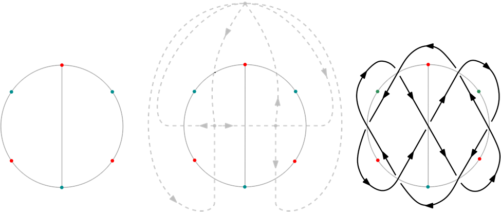
Figure 1. A planar bipartite graph $G$ along with its dual alternating dimap $D$ and its associated positive special alternating link $L_{G}$.

1.3. The BEST Theorem for Eulerian digraphs

Recall that an Eulerian tour of $D$ is a directed cycle that uses each edge of $D$ exactly once. An oriented spanning tree rooted at $r\in V(D)$ is a spanning tree of $D$ such that for each vertex $v\in V(D)$, there is a unique directed path from $v$ to $r$.

A classical theorem in graph theory by de Bruijn, Ehrenfest [23], Smith, and Tutte [22] (named the BEST Theorem for its authors) states that the number of Eulerian tours of an Eulerian digraph $D$ equals the number of oriented spanning trees of $D$ rooted at an arbitrary fixed vertex $r$ of $D$ multiplied by a constant dependent on $D$. In particular, the BEST Theorem implies that:

Theorem 1.2 ([23, 22]).

The number of oriented spanning trees of an Eulerian digraph $D$ is independent of the choice of root.

A $k$-spanning tree rooted at $r\in V(D)$ is a spanning tree of $D$ such that reversing the orientation of exactly $k$ of its edges yields an oriented spanning tree rooted at $r$. With this terminology, $0$-spanning trees coincide with oriented spanning trees. Analogously, an arborescence rooted at $r$ is a spanning tree such that for every $v\in V(D)$, there is a unique directed path from $r$ to $v$, i.e. arborescences of $D$ are precisely $\{|V(D)|-1\}$-spanning trees.

Denote by $c_{k}(D,r)$ the number of $k$-spanning trees rooted at $r$ in the Eulerian digraph $D$. Inspired by the Alexander polynomial of special alternating links, Murasugi and Stoimenow [16] prove the following extension of Theorem 1.2:

Theorem 1.3.

[16] For any $k\in\mathbb{N}$, the number of $k$-spanning trees of an Eulerian digraph $D$ is independent of the choice of root. Moreover, the sequence $c_{0}(D,r)$, $\ldots$, $c_{|V(D)|-1}(D,r)$ is palindromic. Equivalently: $c_{k}(D,r)=c_{|V(D)|-1-k}(D,r)$ for all $k\in\{0,1,\ldots,|V(D)|-1\}$.

We will provide a new proof of Theorem 1.3 which will help us establish connections between the Alexander polynomials of special alternating links and volumes of root polytopes. This connection is outlined in Section 1.5.

1.4. The Alexander polynomial of an Eulerian digraph

Murasugi and Stoimenow [16] define the Alexander polynomial of an Eulerian digraph $D$ (and arbitrary $r\in V(D)$) to be:

(1) $$P_{D}(t)=\sum_{k=0}^{\infty}c_{k}(D,r)t^{k}.$$

The name is justified by Murasugi and Stoimenow’s theorem that for an alternating dimap $D$, the polynomial $P_{D}(t)$ equals the Alexander polynomial of a special alternating link associated to $D$. Recall that an alternating dimap is a planar Eulerian digraph where at each vertex, the edges alternate between coming in and going out as we move cyclically around the vertex.

Theorem 1.4.

[16, Theorem 2] For an alternating dimap $D$, the polynomial $P_{D}(t)$ equals the Alexander polynomial $\Delta_{L_{G}}(-t)$ for the special alternating link $L_{G}$ associated to the planar dual $G$ of $D$.

We provide a proof of Theorem 1.4 in Section 4 which we will utilize in Section 6 to relate the Kauffman and Crowell state models. We note that Murasugi and Stoimenow denote the polynomial $P_{D}$ by $\Delta_{G}$ as they start with an undirected graph $G$ of even valence and then put an arbitrary Eulerian orientation on it. For us, the notation $P_{D}$ will be more convenient.

Previous work of the authors [5, Theorem 1.2] proves that for alternating dimaps $D$, the Alexander polynomial $\Delta_{L_{G}}(-t)$ for the special alternating link $L_{G}$ associated to the planar dual $G$ of $D$ is log-concave. In light of Theorem 1.4, this result can be rephrased as follows for the polynomial  $P_{D}$:

Theorem 1.5.

[5, Theorem 1.2] For any alternating dimap $D$, the coefficients of the polynomial $P_{D}(t)$ form a log-concave sequence with no internal zeros.

We conjecture that Theorem 1.5 generalizes as follows:

Conjecture 1.6.

For any Eulerian digraph $D$, the coefficients of the polynomial $P_{D}(t)$ form a log-concave sequence with no internal zeros.

In Section 5, we prove that Conjecture 1.6 holds for a special family of (not necessarily planar) Eulerian digraphs.

1.5. The polynomial $P_{D}$ in terms of root polytopes

Root polytopes of bipartite graphs were defined and extensively studied by Postnikov [18]. They were related to special alternating links in the works of Kálmán and Murakami [9] and Kálmán and Postnikov [10]. Tóthmérész [21] recently generalized Postnikov’s definition of a root polytope to all oriented co-Eulerian matroids (see Section 3 for definitions). Using this generalization, we connect the polynomial $P_{D}(t)$, as defined in equation (1), to volumes of root polytopes of oriented co-Eulerian matroids:

Theorem 1.7.

Let $D$ be an Eulerian digraph, and let $M$ be the oriented graphic matroid associated to $D$. Let $A$ be a totally unimodular matrix representing $M^{*}$, the oriented dual of $M$, and let $m$ be the size of a basis of $M^{*}$. Then

(2) $$P_{D}(t)=\sum_{H\text{ has property *}}Vol(Q_{H})(t-1)^{\#col(H)-m}$$

where a matrix $H$ has property * if it is obtained by deleting a set of columns from $A$ without decreasing the rank of the matrix.

The right-hand side of equation (2) was previously studied by Li and Postnikov [12] in the context of computing volumes of slices of zonotopes. Our proof techniques for Theorem 1.7 are different from Li and Postnikov’s [12] approach. We note the following interesting corollary for Alexander polynomials of special alternating links:

Corollary 1.8.

The Alexander polynomial $\Delta_{L_{G}}(-t)$ of the special alternating link associated to the planar bipartite graph $G$ can be expressed as:

(3) $$\Delta_{L_{G}}(-t)=\sum_{\begin{subarray}{c}H\subset G\\ H\text{ connected}\end{subarray}}Vol(Q_{H})(q-1)^{|E(H)|-|V(G)|+1}.$$

1.6. On the Kauffman and Crowell state models of the Alexander polynomial

The Alexander polynomial was initially defined by James Alexander II as a determinant [1]. Crowell, in 1959, gave the first combinatorial state model for Alexander polynomials of alternating links [3]. In John Conway’s paper [2], the Conway polynomial was introduced which satisfies a skein relation and is related to the Alexander polynomial by a substitution. In 1982, Kauffman defined the notion of states of a link universe, obtained from a link diagram. Originally, these states were used to compute a polynomial that could be specialized to the Conway polynomial. Later, in the most recent edition of [11], released in 2006, Kauffman described a means of using this combinatorial state model to directly compute the Alexander polynomial of any link.

Theorem 1.4, Murasugi and Stoimenow’s result expressing $P_{D}$ in terms of $k$-spanning trees for alternating dimaps $D$, is based on Kauffman’s model. We can view Theorem 1.4 as another way of expressing the Kauffman states in the special alternating link case. On the other hand, the present authors work establishing Fox’s conjecture for special alternating links, as in Theorem 1.5, is based on and heavily inspired by the Crowell state model for alternating links. It is, thus, natural to wonder about a weight-preserving combinatorial bijection between Crowell’s and Kauffman’s models. In Theorem 6.5, we construct such a bijection between the two models in the case of special alternating links.

Roadmap of the paper. In Section 2, we study the enumeration of $k$-spanning trees of Eulerian digraphs which we use in Section 3 to prove Theorem 1.7. In Section 4, we show that for alternating dimaps $D$, $P_{D}(t)$ is the Alexander polynomial of a special alternating link. The proof we give is inspired by Murasugi and Stoimenow’s proof but is written in a graph theoretic language. In Section 5, we discuss possible generalizations of Fox’s long-standing conjecture that the sequence of absolute values of coefficients of the Alexander polynomial of an alternating link is unimodal. We conclude in Section 6 by constructing an explicit weight preserving bijection between the Crowell and Kauffman states of a special alternating link.

Instead of having a lengthy background section, we will include the necessary background throughout the paper.

2. On $k$-spanning trees of Eulerian digraphs

In this section, we study $k$-spanning trees of Eulerian digraphs, as defined in Section 1.3. We will leverage the results from this section in Section 3 in order to connect the Alexander polynomials of Eulerian digraphs to volumes of root polytopes of oriented co-Eulerian matroids.

Recall from the introduction that $c_{k}(D,r)$ denotes the number of $k$-spanning trees rooted at $r$ in the Eulerian digraph $D$. We will give an alternative proof of the following theorem of Murasugi and Stoimenow:

Theorem 1.3.

([16, Proposition 1]) For any $k\in\mathbb{N}$, the number of $k$-spanning trees of an Eulerian digraph $D$ is independent of the choice of root. Moreover, the sequence $c_{0}(D,r)$, $\ldots$, $c_{|\operatorname{V}(D)|-1}(D,r)$ is palindromic. Equivalently: $c_{k}(D,r)=c_{|\operatorname{V}(D)|-1-k}(D,r)$ for all $k\in\{0,1,\ldots,|\operatorname{V}(D)|-1\}$.

To prove Theorem 1.3, we make use of the BEST Theorem (see Section 1.3) and some of its consequences.

Theorem 2.1.

([19, Theorem 10.2], [22, 23]) Let $D$ be an Eulerian digraph, and fix any edge $e\in\operatorname{E}(D)$ such that $\operatorname{init}(e)=r$. Let $\epsilon(D,e)$ denote the number of Eulerian tours of $D$ beginning with $e$. Then

$$\epsilon(D,e)=c_{0}(D,r)\prod_{u\in\operatorname{V}(D)}(\operatorname{outdeg}(u)-1)!$$

Theorem 1.2.

([19, Corollary 10.3], [22, 23]) For any Eulerian digraph $D$, $c_{0}(D,r)$ is independent of the root $r\in\operatorname{V}(D)$.

Let $D^{T}$ denote the transpose of $D$: the digraph obtained by reversing the direction of each edge in $D$.

Corollary 2.2.

For any Eulerian digraph $D$ and $r\in\operatorname{V}(D)$, $c_{0}(D,r)=c_{0}(D^{T},r)$. In particular, $c_{0}(D,r)=c_{|\operatorname{V}(D)|-1}(D,r)$.

Proof.

Observe that the Eulerian tours of $D^{T}$ are precisely the Eulerian tours of $D$ with the edges listed in reverse. In particular, if $e\in\operatorname{E}(D)$ has initial vertex $r$, then $\epsilon(D,e)=\epsilon(D^{T},f)$ for any $f\in\operatorname{E}(D^{T})$ with $\operatorname{init}(f)=r$. Theorem 2.1 therefore implies that $c_{0}(D,r)=c_{0}(D^{T},r)$.

The second statement follows by observing that $0$-spanning trees of $D$ (oriented spanning trees) are precisely $(|V(D)|-1)$-spanning trees (arborescences) of $D^{T}$ and vice-versa. ∎

We note that Corollary 2.2 also follows from [21, Theorem 4.9].

For an arbitrary digraph $D$ and subset $E^{\prime}\subset E(D)$, let $D\setminus E^{\prime}$ denote the graph obtained from $D$ by deleting the edges in $E^{\prime}$, and let $D/E^{\prime}$ denote the graph obtained from $D$ by contracting the edges in $E^{\prime}$. A minor of $D$ is any graph which can be obtained from $D$ by deleting and/or contracting edges.

Theorem 2.3.

Let $D$ be an Eulerian digraph, and fix any $r\in V(D)$. Then

$$c_{k}(D,r)=\sum_{i=0}^{k}(-1)^{i}\sum_{\begin{subarray}{c}\text{\emph{acyclic} }E^{\prime}\subset E(D)\\ |E^{\prime}|=k-i\end{subarray}}\binom{|V(D)|-1-(k-i)}{i}c_{0}(D/E^{\prime},r)$$

Proof.

Observe that if $T$ is a $0$-spanning tree in $D/E^{\prime}$ for some acyclic $E^{\prime}\subset E(D)$, then $T_{D}:=(\operatorname{V}(D),E(T)\cup E^{\prime})$ is an $i$-spanning tree in $D$ rooted at $r$ for some $0\leq i\leq k$. Similarly, if $T_{D}$ is an $i$-spanning tree in $D$ and $E_{\text{away}}$ is the set of edges of $T_{D}$ directed away from the root, then $T_{D}/E^{\prime}$ is a $0$-spanning tree in $D/E^{\prime}$ for any acyclic $E^{\prime}\supset E_{\text{away}}$. We can thus write

$$c_{k}(D,r)=\sum_{\begin{subarray}{c}\text{acyclic }E^{\prime}\subset E(D)\\ |E^{\prime}|=k\end{subarray}}c_{0}(D/E^{\prime},r)-\sum_{\begin{subarray}{c}\text{acyclic }E^{\prime}\subset E(D)\\ |E^{\prime}|=k\end{subarray}}c_{<k}(D,r)$$

where $c_{<k}(D,r)$ is the number of $0$-spanning trees $T$ in $D/E^{\prime}$ such that there exists $e\in E^{\prime}$ where $E(T)\cup\{e\}$ forms a 0-spanning tree in $D/(E^{\prime}-\{e\})$. Using inclusion-exclusion, we rewrite this as follows:

$$c_{k}(D,r)=\sum_{\begin{subarray}{c}\text{acyclic }E^{\prime}\subset E(D)\\ |E^{\prime}|=k\end{subarray}}c_{0}(D/E^{\prime},r)-\sum_{\begin{subarray}{c}\text{acyclic }E^{\prime}\subset E(D)\\ |E^{\prime}|=k\end{subarray}}\sum_{i=1}^{k}\sum_{\begin{subarray}{c}F\subset E^{\prime}\\ |F|=i\end{subarray}}(-1)^{i-1}c_{0}(D/(E^{\prime}-F),r).$$

Observe that for any subset $F^{\prime}\subset E(D)$ with $|F^{\prime}|=k-i$ and any $0$-spanning tree $T$ in $D/F^{\prime}$, contracting any $i$ edges of $T$ produces a $0$-spanning tree of $D/E^{\prime}$ for some $E^{\prime}$ with $|E^{\prime}|=k$. Relabeling $F^{\prime}:=E^{\prime}-F$ in the above equation thus yields

$$c_{k}(D,r)=\sum_{\begin{subarray}{c}\text{acyclic }E^{\prime}\subset E(D)\\ |E^{\prime}|=k\end{subarray}}c_{0}(D/E^{\prime},r)-\sum_{i=1}^{k}(-1)^{i-1}\sum_{\begin{subarray}{c}\text{acyclic }F^{\prime}\subset E(D)\\ |F^{\prime}|=k-i\end{subarray}}\binom{|V(D/F^{\prime})|-1}{i}c_{0}(D/F^{\prime},r).$$

Since $|V(D/F^{\prime})|=|V(D)|-(k-i)$, we can relabel and combine the sums to obtain

$$c_{k}(D,r)=\sum_{i=0}^{k}(-1)^{i}\sum_{\begin{subarray}{c}\text{acyclic }E^{\prime}\subset E(D)\\ |E^{\prime}|=k-i\end{subarray}}\binom{|V(D)|-1-(k-i)}{i}c_{0}(D/E^{\prime},r).$$

∎

Theorem 2.4.

For any Eulerian digraph $D$, $c_{k}(D,r)=c_{k}(D^{T},r)$.

Proof.

Corrolary 2.2 implies that this holds when $k=0$. Since Theorem 2.3 expresses $c_{k}(D,r)$ entirely in terms of $c_{0}(H,r)$ for Eulerian minors $H$ of $D$, this result follows immediately. ∎

Theorem 1.3.

For any Eulerian digraph $D$, $c_{k}(D,r)$ is independent of the root $r$, and the sequence $c_{0}(D,r)$, $\ldots$, $c_{|V(D)|-1}(D,r)$ is palindromic.

Proof.

Since $k$-spanning trees of $D$ are precisely $(|V(D)|-1-k)$-spanning trees of $D^{T}$, this follows immediately from Theorems 1.2 and 2.4. ∎

3. $P_{D}(t)$ in terms of volumes of Root Polytopes of oriented co-Eulerian matroids

In this section, we prove Theorem 1.7. Before we do so, we review the work of Tóthmérész [21] on root polytopes of co-Eulerian matroids. We follow parts of her exposition.

A matroid $M$ is said to be regular if it is representable by a totally unimodular matrix, i.e. a matrix whose subdeterminants are all either $1$, $0$, or $-1$. Let $A$ denote such a matrix and $\{a_{1},\dots,a_{m}\}$ its columns. For each circuit $C=\{i_{1},\dots,i_{j}\}$ of a regular matroid with a corresponding linear dependence relation $\sum_{k=1}^{j}\lambda_{k}a_{i_{k}}=0$ of columns of $A$, we may partition its elements into two sets: $C^{+}=\{i_{k}\ |\ \lambda_{k}>0\}$ and $C^{-}=\{i_{k}\ |\ \lambda_{k}<0\}$. Observe that scaling the expression $\sum_{k=1}^{j}\lambda_{k}a_{i_{k}}$ by a nonzero constant potentially interchanges $C^{+}$ and $C^{-}$, but the partition of $C$ into these two sets is well-defined up to this exchange. In this way, regular matroids are oriented.

Two regular oriented matroids $M_{1}$ and $M_{2}$ on groundset $E$ have mutually orthogonal signed circuits if for each pair of signed circuits $C_{1}={C_{1}}^{+}\sqcup{C_{1}}^{-}$ and $C_{2}={C_{2}}^{+}\sqcup{C_{2}}^{-}$ of $M_{1}$ and $M_{2}$, respectively, either $C_{1}\cap C_{2}=\emptyset$, or $({C_{1}}^{+}\cap{C_{2}}^{+})\cup({C_{1}}^{-}\cap{C_{2}}^{-})$ and $({C_{1}}^{+}\cap{C_{2}}^{-})\cup({C_{1}}^{-}\cap{C_{2}}^{+})$ are both nonempty. Every regular oriented matroid $M$ admits a unique dual oriented matroid $M^{*}$ such that $M$ and $M^{*}$ have mutually orthogonal signed circuits.

Definition 3.1 ([21] Definition 3.4).

A regular oriented matroid is co-Eulerian if for each circuit $C$, $|C^{+}|=|C^{-}|$.

Lemma 3.2 ([21] Claim 3.5).

For an Eulerian digraph $D$, the oriented dual $M^{*}$ of the graphic matroid of $D$ is a co-Eulerian regular oriented matroid.

With this foundation, Tóthmérész introduces the following definition and results.

Definition 3.3 ([21] Definition 3.1).

Let $A$ be a totally unimodular matrix with columns $a_{1},\dots,a_{m}$. The root polytope of $A$ is the convex hull $\mathcal{Q}_{A}:=\emph{conv}(a_{1},\dots,a_{m})$.

Tóthmérész demonstrates that for any pair of totally unimodular matrices $A$ and $A^{\prime}$ representing the same regular oriented matroid $M$, there is a lattice point-preseving linear bijection between $t\cdot\mathcal{Q}_{A}$ and $t\cdot\mathcal{Q}_{A^{\prime}}$ for any $t\in\mathbb{Z}$. In this way, the definition of a root polytope can be extended to regular oriented matroids. The set of arborescences of an Eulerian digraph yields a triangulation of the root polytope of the dual matroid. Recall that an arborescence of $D$ rooted at $r\in\operatorname{V}(D)$ is a directed subgraph $A$ such that for each other vertex $v$ of $D$, there is a unique directed path in $A$ from $r$ to $v$.

Proposition 3.4 ([21] Proposition 3.8).

For a regular oriented matroid represented by a totally unimodular matrix $A$ and a basis $B=\{i_{1},\dots,i_{j}\}$, the simplex $\Delta_{B}:=\emph{conv}(a_{i_{1}},\dots,a_{i_{j}})$ is unimodular. That is, its normalized volume is $1$.

Theorem 3.5 ([21] Theorem 4.1).

Let $D$ be an Eulerian digraph, and let $A$ be any totally unimodular matrix representing the oriented dual of the oriented graphic matroid of $D$. Let $r\in V(D)$ and $\mathcal{D}=\{B\subset E(D)\ |\ E(D)-B\ \text{is an arborescence of}\ D\ \text{rooted at}\ r\}$. Then $\{\Delta_{B}\ |\ B\in\mathcal{D}\}$ is a triangulation of $\mathcal{Q}_{A}$.

Corollary 3.6 ([21]).

Let $D$ be an Eulerian digraph, and let $A$ be any totally unimodular matrix representing the oriented dual of the oriented graphic matroid of $D$. Let $r\in V(D)$. Then

$$\emph{Vol}(\mathcal{Q}_{A})=c_{0}(D,r).$$

As a consequence, we may reformulate our Theorem 2.3 in terms of volumes of root polytopes.

Corollary 3.7.

For an Eulerian digraph $D$, let $H_{D}$ denote a totally unimodular matrix representing the oriented dual of the graphic matroid of $D$.

$$c_{k}(D,r)=\sum_{i=0}^{k}(-1)^{i}\sum_{\begin{subarray}{c}\text{acyclic }E^{\prime}\subset E(D)\\ |E^{\prime}|=k-i\end{subarray}}\binom{|V(D)|-1-(k-i)}{i}\emph{Vol}(\mathcal{Q}_{H_{D/E^{\prime}}}).$$

We are now ready to prove:

Theorem 1.7.

Let $D$ be an Eulerian digraph, and let $M$ be the oriented graphic matroid associated to $D$. Let $A$ be a totally unimodular matrix representing $M^{*}$, the oriented dual of $M$, and let $m$ be the size of a basis of $M^{*}$. Then

(4) $$P_{D}(t)=\sum_{k=0}^{\infty}c_{k}(D,r)t^{k}=\sum_{H\text{ has property *}}Vol(Q_{H})(t-1)^{\#col(H)-m}$$

where a matrix $H$ has property * if it is obtained by deleting a set of columns from $A$ without decreasing the rank of the matrix.

Proof.

Note that if $k>|V(D)|-1$, then $c_{k}(D,r)=0$ since a spanning tree in $D$ has $|V(D)|-1$ edges. Since $\#col(A)-m=|V(D)|-1$ (both sides compute the size of a basis of $M$), the right-hand side also has no terms of degree greater than $|V(D)|-1$.
Using a binomial expansion, the desired result is equivalent to

$$c_{k}(D,r)=\sum_{i=0}^{\#col(A)-k-m}\sum_{\begin{subarray}{c}H\text{ with property *}\\ \#col(H)=k+m+i\end{subarray}}(-1)^{i}\binom{k+i}{i}Vol(Q_{H})$$

for all $k\leq|V(D)|-1$. Since $c_{k}(D,r)=c_{|V(D)|-1-k}(D,r)$, this is also equivalent to

$$\begin{split}c_{k}(D,r)&=\sum_{i=0}^{\#col(A)-|V(D)|+k-m+1}\sum_{\begin{subarray}{c}H\text{ with property *}\\ \#col(H)=|V(D)|-1-k+m+i\end{subarray}}(-1)^{i}\binom{|V(D)|-1-k+i}{i}Vol(Q_{H})\\ &=\sum_{i=0}^{k}\sum_{\begin{subarray}{c}H\text{ with property *}\\ \#col(H)=\#col(A)-k+i\end{subarray}}(-1)^{i}\binom{|V(D)|-1-k+i}{i}Vol(Q_{H})\end{split}$$

Recall that by standard results in matroid theory, deleting elements of $M^{*}$ (or columns of $A$) is equivalent to contracting the corresponding elements in $M$. Furthermore, the set of columns we remove from $A$ to form $H$ are disjoint to a basis of $M^{*}$ (since removing them did not decrease the rank of the matrix), so these columns form an independent set of $M$. Since the independent sets in the graphic matroid of $D$ are precisely acyclic subsets of edges of $D$, the desired result is equivalent to

$$c_{k}(D,r)=\sum_{i=0}^{k}(-1)^{i}\sum_{\begin{subarray}{c}\text{acyclic }E^{\prime}\subset E(D)\\ |E^{\prime}|=k-i\end{subarray}}\binom{|V(D)|-1-(k-i)}{i}\emph{Vol}(\mathcal{Q}_{H_{D/E^{\prime}}})$$

which holds by Corollary 3.7. ∎

Both Theorem 1.7 and the following corollary are closely related to the beautiful unpublished work of Li and Postnikov [12].

Corollary 1.8.

The Alexander polynomial $\Delta_{L_{G}}(-t)$ of the special alternating link associated to the planar bipartite graph $G$ can be expressed as:

(5) $$\Delta_{L_{G}}(-t)=\sum_{\begin{subarray}{c}H\subset G\\ H\text{ connected}\end{subarray}}Vol(Q_{H})(q-1)^{|E(H)|-|V(G)|+1}.$$

Proof.

Note that for any alternating dimap $D$ whose planar dual is the bipartite graph $G$, Theorem 1.7 specializes to:

(6) $$P_{D}(t)=\sum_{\begin{subarray}{c}H\subset G\\ H\text{ connected}\end{subarray}}Vol(Q_{H})(q-1)^{|E(H)|-|V(G)|+1}.$$

Then Corollary 1.8 follows readily from Theorem 1.4 and equation (6). ∎

4. $P_{D}(t)$ as the Alexander polynomial of special alternating links

As mentioned in the introduction, the polynomial $P_{D}(t)$ is the Alexander polynomial of a special alternating link when $D$ is an alternating dimap. This was established by Murasugi and Stoimenow [16]. We give a proof here for completeness. Our proof is closely related to the one they provided. We will use parts of our proof of Theorem 1.4 to establish our weight-preserving bijection between the Crowell and Kauffman state models in Section 6.

Theorem 1.4.

[16, Theorem 2] For an alternating dimap $D$, the Alexander polynomial of $D$, $P_{D}(t)$, equals the Alexander polynomial $\Delta_{L_{G}}(-t)$ for the special alternating link $L_{G}$ associated to the planar dual $G$ of $D$. In other words:

$$\Delta_{L_{G}}(-t)\sim\sum_{k=0}^{|\operatorname{V}(D)|-1}c_{k}(D,r)t^{|\operatorname{V}(D)|-1-k}.$$

Theorem 1.4 is stated in [16] as $\Delta_{L_{G}}(-t)\sim P_{D}(t)$. By Theorem 1.3, $P_{D}(t)$ is palindromic; therefore, $\Delta_{L_{G}}(-t)\sim P_{D}(t)$ is equivalent to $\Delta_{L_{G}}(-t)\sim\sum_{k=0}^{|\operatorname{V}(D)|-1}c_{k}(D,r)t^{|\operatorname{V}(D)|-1-k}$ which is what we state in Theorem 1.4.

Before proving Theorem 1.4, we present Kauffman’s state model.

4.1. Kauffman’s state model

The State Summation, introduced by Kauffman [11], describes the Alexander polynomial as a sum over weights of decorations of a link diagram, called states [11]. To form a state, one begins with a (not necessarily alternating) link diagram and marks two (arbitrary) adjacent regions. Each meeting between a nonmarked region and a crossing is labeled as follows:

Each state is then a bijection between crossings in the diagram and the nonmarked regions so that each crossing is mapped to one of the four regions it meets. This bijection is presented diagrammatically, as in Figure 2, via state markers. For each state $S$, there is a signed monomial $\langle L|S\rangle$, computed as the product of the weights corresponding to the marked region at each crossing.

Kauffman defines a black hole to be any state marker of the form below.

Let $b(S)$ be the number of black holes in a fixed state $S$.

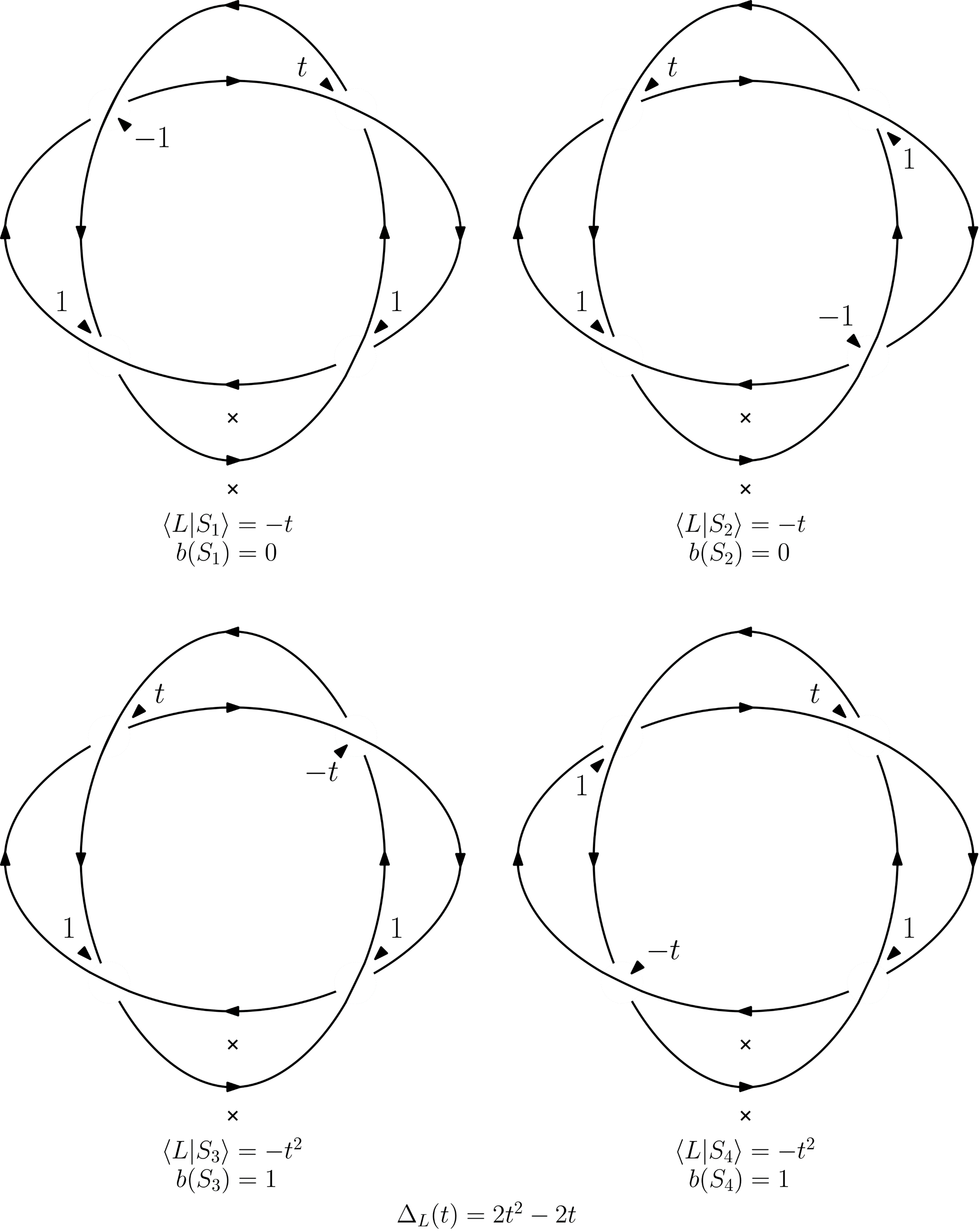
Figure 2. The four states of the positive $K(2,2)$ along with their monomial weights and the resulting Alexander polynomial.

Theorem 4.1 ([11] pg. 176).

$\Delta_{L}(t)\sim\sum_{S}\langle L|S\rangle(-1)^{b(S)}$.

Kauffman also interprets these states graph theoretically. Given any diagram of a link, 2-color its regions so that at each crossing, no two regions of the same color are adjacent. Partition the set of regions according to color into sets $V$ and $V^{\prime}$ where $V^{\prime}$ is the set containing the exterior. Given a link diagram, the checkerboard graph of the link is the graph with vertex set $V$ where two vertices $r,r^{\prime}\in V$ are connected by an edge if and only if their corresponding regions meet at a crossing in the link diagram. We will denote the checkerboard graph by $G$ and its planar dual by $G^{*}$. Notice that $G^{*}$ may be constructed in the same way by taking the vertex set to be $V^{\prime}$. We refer to $G^{*}$ as the checkerboard dual graph.

Kauffman provides a bijection between states of a link diagram and spanning trees of the checkerboard graph (or equivalently, spanning trees of the checkerboard dual). Given a state $S$, one draws an edge between vertices in its associated tree if and only if they are separated by a crossing whose state marker points from the region corresponding to one vertex to the region corresponding to the other. In this way, a state identifies a pair of spanning trees that we refer to as dual spanning trees: one in $G$ and one in $G^{*}$. We note that these dual spanning trees are not planar duals of each other; rather, they correspond to bases in the graphic matroids of $G$ and $G^{*}$ which are complements of one another.

Conversely, given a spanning tree $T$ of $G$ and its dual spanning tree $T^{\prime}$ in $G^{*}$ (which consists of the edges in $E(G^{*})$ which do not correspond to edges in $E(T)$, see Figure 3), one recovers a state by assigning edge orientations that make $T$ and $T^{\prime}$ oriented spanning trees rooted at the vertices corresponding to the two adjacent marked regions. When a directed edge is incident to a crossing, place a state marker pointing into that crossing from the region corresponding to the initial vertex of the edge, as in Figure 3.

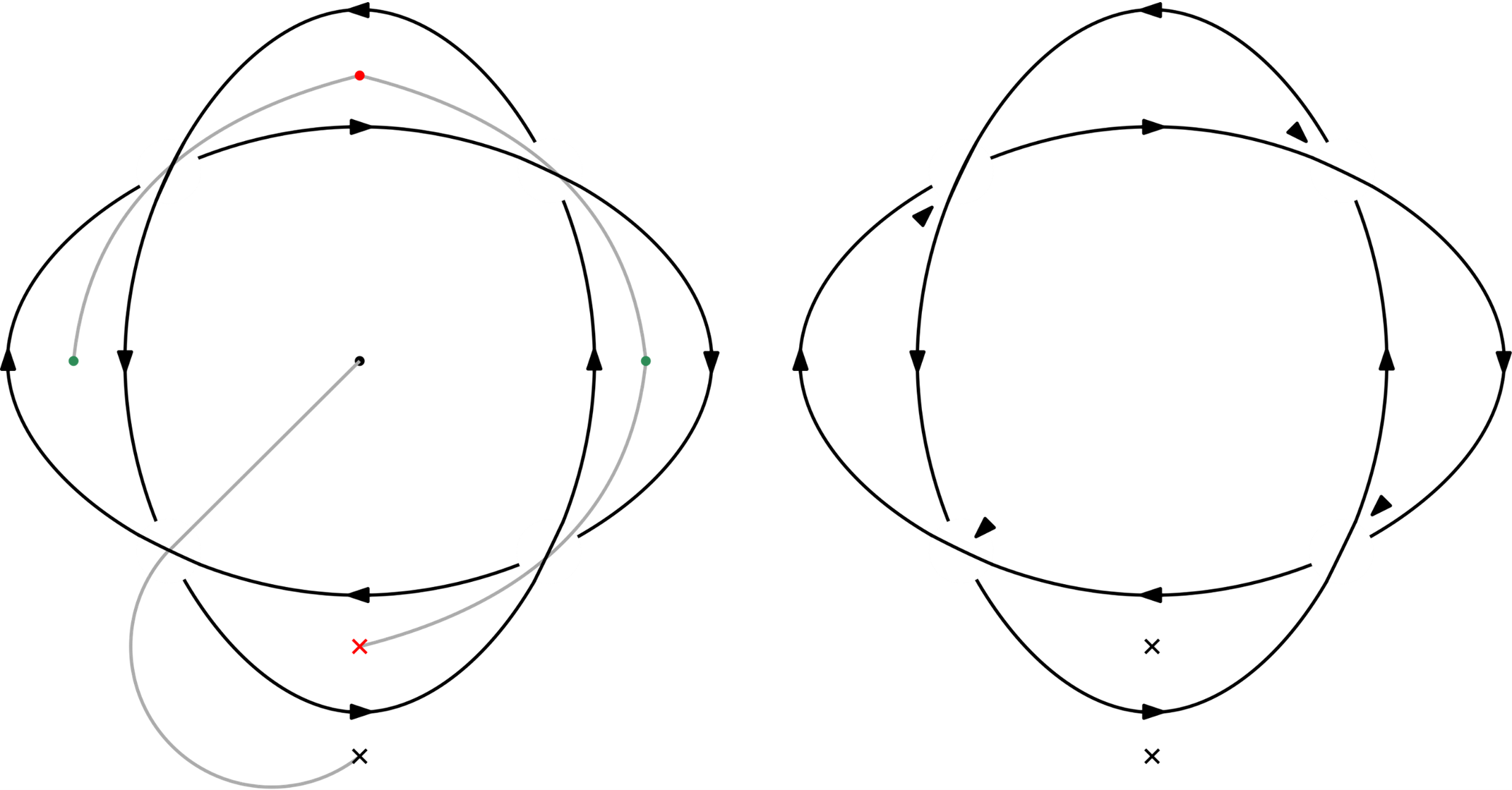
Figure 3. A tree in the checkerboard graph of the positive $K(2,2)$ and its dual along with the corresponding state.

4.2. Proof of Theorem 1.4

To prove Theorem 1.4, we require the following lemma which we will also utilize in our weight-preserving bijection between the Crowell and Kauffman models.

Lemma 4.2.

Fix a bipartite graph $G$ with color classes $A$ and $B$, and let $r^{\prime}\in\operatorname{V}(G)$. Let $S$ be any spanning tree of $G$. Orient the edges of $S$ so that it is an oriented spanning tree rooted at $r^{\prime}$. The number of oriented edges $(a,b)\in\operatorname{E}(S)$ where $a\in A$ and $b\in B$ is independent of the choice of $S$.

Proof.

We first consider the case where $G$ is a bipartite cycle. It is easy to see that the number of edges $(a,b)$ with $a\in A$ and $b\in B$ is $|A|$ if $r^{\prime}\in B$ and $|A|-1$ if $r^{\prime}\in A$. In either case, this is independent of the choice of spanning tree.

Next, let $G$ be an arbitrary bipartite graph, and let $r^{\prime}\in\operatorname{V}(G)$. Any two spanning trees of $G$ are connected by a sequence of edge exchanges. It, thus, suffices to show that if $S$ and $S^{\prime}$ are two spanning trees related by a single edge exchange and oriented so that they are oriented spanning trees rooted at $r^{\prime}$, then they have the same number of oriented edges $(a,b)$ with $a\in A$ and $b\in B$.

Notice that $S\cup S^{\prime}$ contains a single undirected cycle $C$ with distinct edges $e,e^{\prime}\in\operatorname{E}(C)$ such that $(S\cup S^{\prime})\setminus\{e\}=S$ and $(S\cup S^{\prime})\setminus\{e^{\prime}\}=S^{\prime}$. Consider the forest $(S\cup S^{\prime})\setminus C$. The component of this forest containing $r^{\prime}$ intersects $C$ in at least one vertex. Indeed, it must intersect $C$ in exactly one vertex $s$ – if it intersected $C$ in at least two distinct vertices, then $S\cup S^{\prime}$ would admit two distinct (undirected) cycles. Treating $C\setminus\{e\}$ and $C\setminus\{e^{\prime}\}$ as oriented spanning trees rooted at $s$, the above argument shows that they have the same number of oriented edges $(a,b)$ where $a\in A$ and $b\in B$. Since $S\setminus C=S^{\prime}\setminus C$, we conclude that $S$ and $S^{\prime}$ have the same number of oriented edges $(a,b)$ where $a\in A$ and $b\in B$. ∎

For the remainder of this section, we will let $A$ and $B$ denote the color classes of $G$ corresponding to regions in the diagram of $L_{G}$ with counterclockwise oriented boundary and clockwise oriented boundary, respectively.

Lemma 4.3.

Suppose each crossing of $L_{G}$ is labeled as in Kauffman’s model. Every meeting between a crossing and a region associated with an element of $A$ is labeled $t$, and every meeting between a crossing and a region associated with an element of $B$ is labeled $1$. (See Figure 5).

Proof.

The requirements that every crossing of $L_{G}$ is positive, that the segments of $L_{G}$ surrounding regions in $A$ spin clockwise, and that the segments of $L_{G}$ surrounding regions in $B$ spin counterclockwise imply that each meeting between an edge of $G$ and a crossing of $L_{G}$ has the form shown in Figure 5. The definition of Kauffman’s model, thus, yields the desired result. ∎

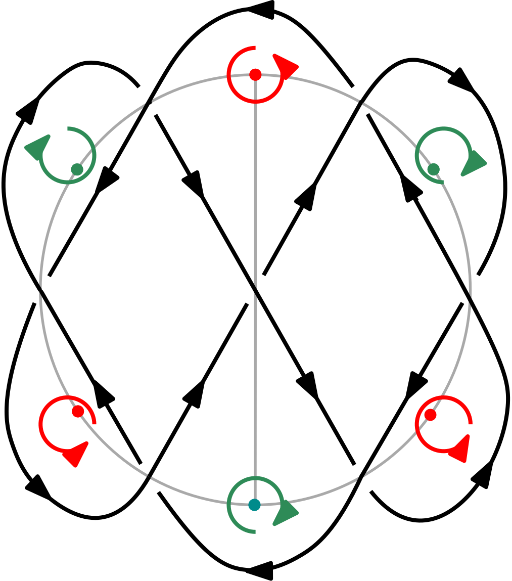
Figure 4. An example of a special alternating link with edge orientations around each vertex of the checkerboard graph indicated.

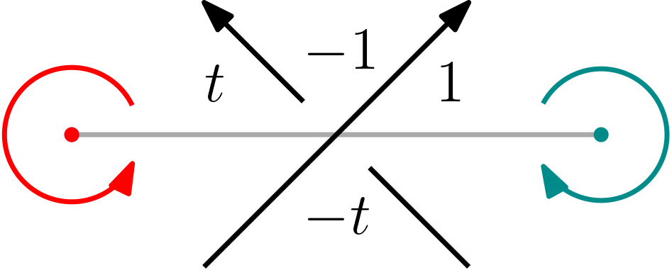
Figure 5. The Kauffman weights at each region meeting a crossing with an edge in $G$.

With this foundation, we proceed with the proof of Theorem 1.4.

Proof of Theorem 1.4. Given an alternating dimap $D$, we construct and orient the link $L_{G}$ as in Section 1.2. Supoose $L_{G}$ is labeled as in Kauffman’s model. By construction, whenever an edge of $D$ meets a crossing in $L_{G}$, the edge points from a region labeled $-t$ into a region labeled $-1$ (as shown in Figure 6).

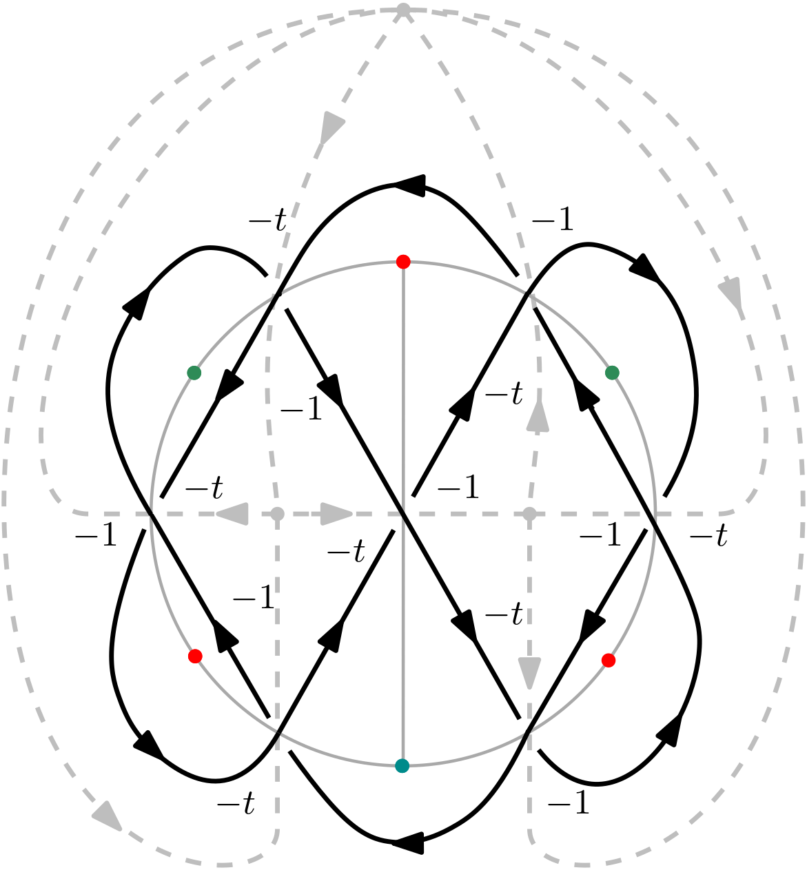
Figure 6. A special alternating link $L_{G}$ with $D$ superimposed. Here, edges of $D$ are weighted as in Kauffman’s model.

Now, let $r^{\prime}\in\operatorname{V}(G)$ and $r\in\operatorname{V}(D)$ denote vertices corresponding to adjacent regions in the link diagram $L_{G}$. Consider dual spanning trees $T$ and $T^{\prime}$ of $D$ and $G$, respectively. Recall that when forming a state using the dual trees $T^{\prime}$ and $T$ with roots $r^{\prime}$ and $r$, an edge $e$ of $T$ corresponds to a state marker with label $-t$ if and only if when $T$ is rooted at $r$, $e$ points from a region labeled $-t$ into a region labeled $-1$ at its corresponding crossing (otherwise, the state marker has label $-1$). By the above construction, this occurs precisely when the orientation of $e$ yielded by rooting $T$ at $r$ matches the orientation of $e$ in $D$.

Let $\operatorname{E}_{\text{away}}(T)$ denote the subset of edges of $T$ such that reversing the orientation of each element of $\operatorname{E}_{\text{away}}(T)$ makes $T$ an oriented spanning tree. The edges of $\operatorname{E}_{\text{away}}(T)$ are precisely those whose orientations after rooting $T$ at $r$ are opposite their orientation in $D$. This implies that $T$ contributes monomial weight $t^{|\operatorname{E}(T)\setminus\operatorname{E}_{\text{away}}(T)|}$ to $P_{D}(t)$; in other words, if $T$ is a $k$-spanning tree, it contributes weight $t^{|\operatorname{V}(G)|-1-k}$.

Notice that an edge in $T^{\prime}$ contributes nontrivially to its associated monomial if and only if it is directed away from a vertex in $A$. In particular, by Lemma 4.3, the degree of this monomial is the number of edges $(a,b)$ where $a\in A$ and $b\in B$, when $T^{\prime}$ is rooted at $r$. By Lemma 4.2, this degree $m$ is independent of the choice of spanning tree.

All directed edges of $D$ meet crossings of the original link at black holes. Viewing any edge in $D$ as in Figure 5, the directed edge meets the positive crossing from below where the segments of the link are also oriented upwards. The number of black holes in the state defined by $T$ and $T^{\prime}$ is thus $|\operatorname{E}_{\text{away}}(T)|$. As such, no cancellation occurs in the state summation of a special alternating link.

We thus conclude that if $T$ is a $k$-spanning tree and $S$ is the state given by $T$ and $T^{\prime}$, then $\langle L_{G}|S\rangle=t^{m}t^{|\operatorname{V}(G)|-1-k}$, and we can write

$$\Delta_{L_{G}}(-t)\sim\sum_{S}|\langle L_{G}|S\rangle| =\sum_{k=0}^{|\operatorname{V}(D)|-1}\sum_{S\ \text{such that T is a $k$-spanning tree}}|\langle L_{G}|S\rangle|$$

$$=\sum_{k=0}^{|\operatorname{V}(D)|-1}\sum_{S\ \text{such that T is a $k$-spanning tree}}t^{m}t^{|\operatorname{V}(D)|-1-k}$$

$$=\sum_{k=0}^{|\operatorname{V}(D)|-1}c_{k}(D,r)t^{m}t^{|\operatorname{V}(D)|-1-k}$$

$$\sim\sum_{k=0}^{|\operatorname{V}(D)|-1}c_{k}(D,r)t^{|\operatorname{V}(D)|-1-k}$$

∎

Remark 4.4.

The proof of Theorem 1.4 shows that in the case of special alternating links $L_{G}$, the Alexander polynomial $\Delta_{L_{G}}(-t)=P_{D}(t)$ can be calculated by collecting terms $t^{|\operatorname{E}(T)\setminus\operatorname{E}_{\text{away}}(T)|}$ for each spanning tree $T$ of $D$ (with specified arbitrary root $r$). We will later use the notation $\text{wt}_{K}(T)=t^{|\operatorname{E}(T)\setminus\operatorname{E}_{\text{away}}(T)|}$ where the subscript $K$ indicates that we are dealing with the Kauffman weight for special alternating links.

5. A note on generalizing Fox’s conjecture for special alternating links

We note that Conjecture 1.6 is a generalization of Fox’s Conjecture 1.1 for special alternating links. Recall Conjecture 1.6:

Conjecture 1.6.

For any Eulerian digraph $D$, the coefficients of the polynomial $P_{D}(t)$ form a log-concave sequence with no internal zeros.

While the methods of [5] settled the alternating dimap case of Conjecture 1.6, they cannot readily be adapted to all Eulerian digraphs. We offer here another case in which Conjecture 1.6 holds.

The Laplacian matrix of an Eulerian graph $D$ on the vertex set $[n]=\{1,\ldots,n\}$ is the matrix $L(D)=(l_{i,j})_{i,j\in[n]}$, defined by

$$l_{i,j}=\begin{cases}\operatorname{outdeg}(i)&\text{for}\ i=j\\ |\{e\in E(D)\ :\ $e$\ \text{is an edge from}\ i\ \text{to}\ j\}|&\text{for}\ i\neq j\end{cases}.$$

Let $\overline{L(D)}$ be the reduced Laplacian obtained from $L$ by removing a row and a column (of the same index).

Lemma 5.1 ([16]).

For any Eulerian directed graph, $P_{D}(t)$ can be expressed via the determinantal formula

$$P_{D}(t)=\det(\overline{L(D)}+t\overline{L(D)}^{T}).$$

Recall that a sequence of nonnegative integers $a_{0},\ldots,a_{d}$ is ultra log-concave if

$$\frac{a_{k}^{2}}{{d\choose k}^{2}}\geq\frac{a_{k+1}}{{d\choose{k+1}}}\frac{a_{k-1}}{{d\choose{k-1}}}\text{ for all }0<k<d.$$

In particular, ultra log-concavity implies log-concavity.

Proposition 5.2.

The sequence of coefficients of $P_{D}(t)$ is ultra log-concave for all Eulerian diagraphs $D$ on the vertex set $[n]$ which have the same number of edges going from vertex $i$ to vertex $j$ as from vertex $j$ to vertex $i$ for all $i,j\in[n]$.

Proof.

If $D$ has the same number of edges going from vertex $i$ to vertex $j$ as from vertex $j$ to vertex $i$ for all $i,j\in[n]$, then $\overline{L(D)}$ is symmetric: $\overline{L(D)}^{T}=\overline{L(D)}$. In this case, Lemma 5.1 yields:

$$P_{D}(t)=\det(\overline{L(D)}+t\overline{L(D)}^{T})=(t+1)^{n-1}\det(\overline{L(D)}).$$

Since the sequence of coefficients of $(t+1)^{n-1}$ is ultra log-concave, we achieve the desired result.

∎

We note that in general, ultra log-concavity of the coefficients of $P_{D}(t)$ does not hold. For example, consider the case when $D$ is an oriented three-cycle (see Figure 7). In this case, the sequence of coefficients of $P_{D}(t)$ is $(1,1,1)$ which is not ultra log-concave.

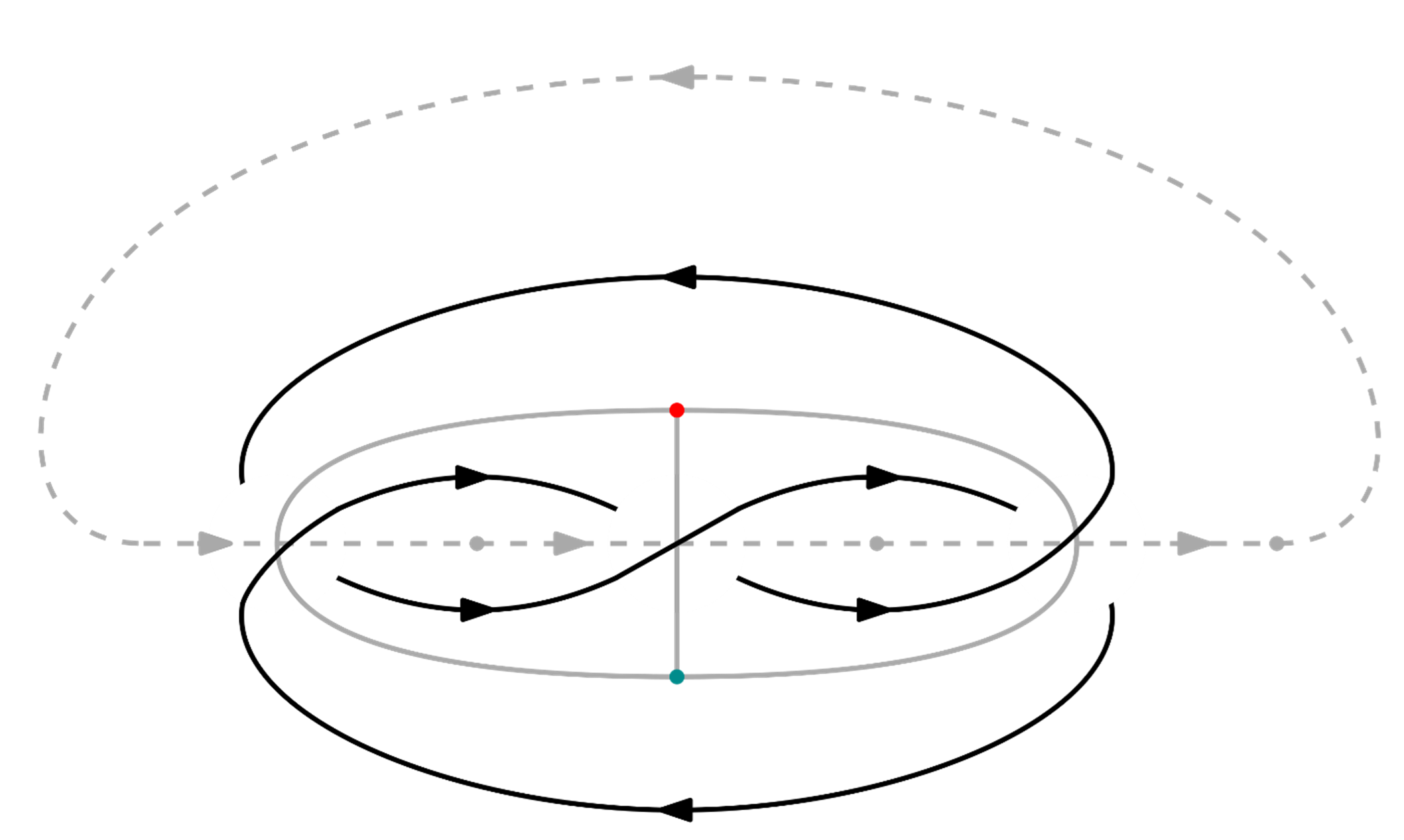
Figure 7. The oriented three-cycle $D$, superimposed on a link diagram of the trefoil knot, and its checkerboard graph.

6. Bijection between the Crowell and Kauffman state models

This section is devoted to relating the first state model for the Alexander polynomial: Crowell’s model [3] to the most well-known one: the Kauffman state model [11]. In Theorem 6.5, we define a weight-preserving bijection between the states of the Crowell model and the states of the Kauffman model for special alternating links.

We will use the following notation throughout Section 6. We denote by $G$ the planar bipartite graph which is the checkerboard graph of the special alternating link $L:=L_{G}$. The alternating dimap $D$ is the directed Eulerian dual of $G$ (see Section 1.2 and Figure 1).

6.1. Crowell’s model

The following combinatorial model for the Alexander polynomial of alternating links is due to Crowell [3]. Recall that a link is alternating if it has an alternating diagram. A diagram is alternating if its undercrossings and overcrossings alternate as we trace it.

Let $\mathcal{G}(L)$ be the planar graph obtained by flattening the crossings of an alternating diagram of $L$: the crossings of $L$ are the vertices of $\mathcal{G}(L)$, and the arcs between the crossings are the edges of $\mathcal{G}(L)$. Note that $\mathcal{G}(L)$ is a planar $4$-regular $2$-face colorable graph. Next, we assign directions and weights to the edges of $\mathcal{G}(L)$ in the following way:

On the left, we see the orientation of the link $L$ in an overcrossing, and on the right, we see how the edges of $\mathcal{G}(L)$ are directed and weighted. Note that the edge orientations assigned to $\overrightarrow{\mathcal{G}(L)}$ are not the same as the orientation of the corresponding components of the link. Denote by $\overrightarrow{\mathcal{G}(L)}$ the oriented weighted graph obtained from $\mathcal{G}(L)$ in this fashion. Let $var(e)$ denote the weight $-t$ or $1$ assigned to the edge $e\in E(\overrightarrow{\mathcal{G}(L)})$. See Figure 8 for a full example.

Recall that an arborescence of $\overrightarrow{\mathcal{G}(L)}$ rooted at $v\in\operatorname{V}(\overrightarrow{\mathcal{G}(L)})$ is a directed subgraph $T$ such that for each other vertex $u$, there is a unique directed path in $T$ from $v$ to $u$. We will denote by $\mathcal{A}_{v}(\overrightarrow{\mathcal{G}(L)})$ the set of arborescences of $\overrightarrow{\mathcal{G}(L)}$ rooted at $v$.

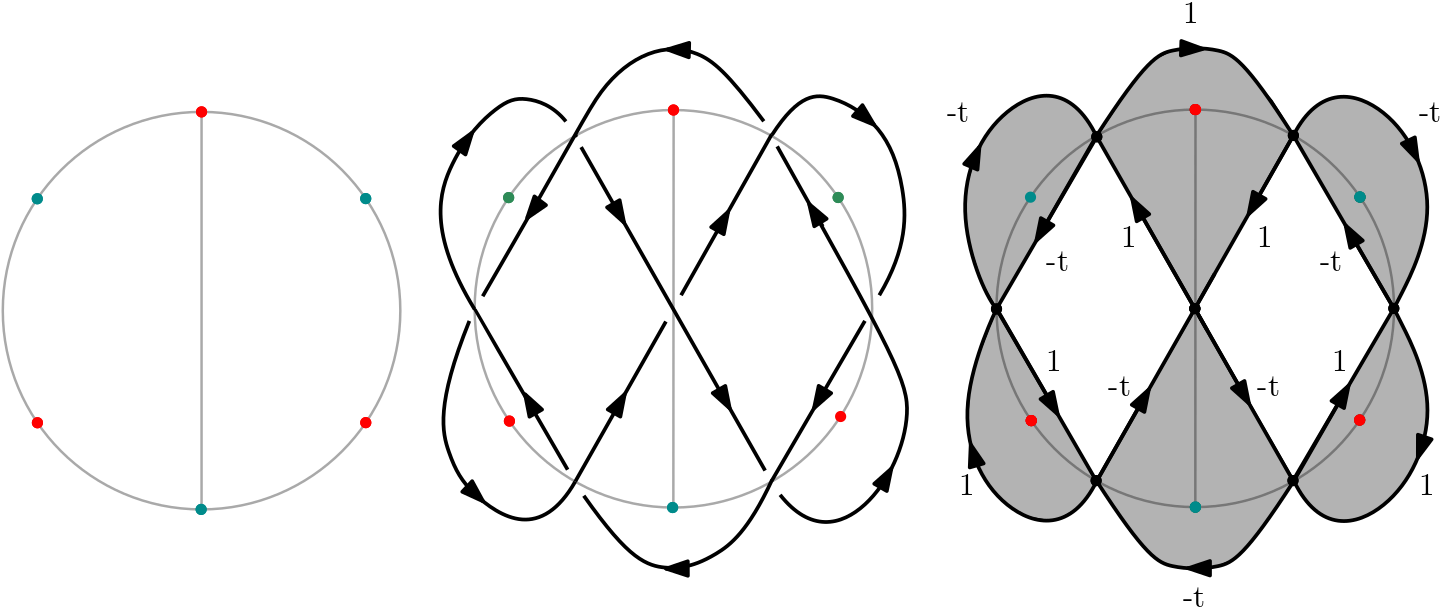
Figure 8. A planar bipartite graph $G$ along with its associated positive special alternating link $L$ and Crowell’s edge weighted digraph $\overrightarrow{\mathcal{G}(L)}.$

Theorem 6.1 ([3] Theorem 2.12).

Given an alternating diagram of the link $L$, fix an arbitrary vertex $v\in V(\overrightarrow{\mathcal{G}(L)})$. The Alexander polynomial of $L$ is:

$$\Delta_{L}(t)\sim\sum_{\begin{subarray}{c}A\in\mathcal{A}_{v}(\overrightarrow{\mathcal{G}(L)})\end{subarray}}\prod_{e\in E(A)}var(e).$$

Remark 6.2.

Theorem 6.1 shows that in the case of alternating links $L$, the Alexander polynomial $\Delta_{L}(t)$ can be calculated by collecting terms $\prod_{e\in E(A)}var(e)$ for each arborescence $A$ of $\overrightarrow{\mathcal{G}(L)}$ (with specified arbitrary root $v$). We will later use the notation $\text{wt}_{C}(A)=\prod_{e\in\operatorname{E}(A)}var(e)$ where the subscript $C$ indicates that we are dealing with the Crowell weight of an arborescence.

6.2. Definition of our weight-preserving bijection

Fix $v\in\operatorname{V}(\overrightarrow{\mathcal{G}(L)})$ and $f_{v}\in\operatorname{E}(\overrightarrow{\mathcal{G}(L)})$ with final vertex $v$. Let $\mathcal{C}(\overrightarrow{\mathcal{G}(L)})$ denote the set of Eulerian tours of $\overrightarrow{\mathcal{G}(L)}$, and let $\mathcal{T}(D)$ denote the set of spanning trees of $D$. Recall that without its edge orientation, $\overrightarrow{\mathcal{G}(L)}$ is the medial graph of $G$ (see Section 1.2). Since $D$ is the planar dual of $G$, $\overrightarrow{\mathcal{G}(L)}$ can equivalently be constructed as the medial graph of $D$. In this section, we will write $v_{e}$ to mean the vertex of $\overrightarrow{\mathcal{G}(L)}$ corresponding to an edge $e\in E(D)$, as in this medial graph construction.

Definition 6.3.

Let $\Phi:\mathcal{T}(D)\rightarrow\mathcal{C}(\overrightarrow{\mathcal{G}(L)})$ be the map which, given $T\in\mathcal{T}(D)$, produces $\Phi(T)$ by the following procedure. At each vertex $v_{e}$ of $\overrightarrow{\mathcal{G}(L)}$, we choose a pairing of incident edges as shown below, depending on whether or not $e$ is in $E(T)$.

On the left, we show an edge $e\in E(D)$ meeting the vertex $v_{e}$ in $\overrightarrow{\mathcal{G}(L)}$. The center diagram shows the choice of edge pairing in $\overrightarrow{\mathcal{G}(L)}$ when $e\in E(T)$, and the right diagram shows the choice of edge pairing in $\overrightarrow{\mathcal{G}(L)}$ when $e\notin E(T)$.

Figure 9 depicts an example of a spanning tree and its image under $\Phi$ interpreted as an Eulerian tour of $\overrightarrow{\mathcal{G}(L)}$.

Definition 6.4.

Let $\Psi_{v,f_{v}}:C(\overrightarrow{\mathcal{G}(L)})\rightarrow\mathcal{A}_{v}(\overrightarrow{\mathcal{G}(L)})$ be the following map. Given an Eulerian tour $C$ of $\overrightarrow{\mathcal{G}(L)}$, $\Psi_{v,f_{v}}(C)$ is the subgraph of $\overrightarrow{\mathcal{G}(L)}$ formed by tracing $C$, starting at the edge $f_{v}$, and at each $u\in\operatorname{V}(\overrightarrow{\mathcal{G}(L)})\setminus{v}$, selecting the first edge incoming to $u$.

An eloquent exposition of the map from Definition 6.4 can be found in Stanley’s account of the BEST Theorem [19]. Applying [19, Theorem 10.2] to $\overrightarrow{\mathcal{G}(L)}^{T}$ with the additional condition that every vertex of $\overrightarrow{\mathcal{G}(L)}$ has outdegree $2$, we readily obtain that $\Psi_{v,f_{v}}$ is a bijection. Recall that $\overrightarrow{\mathcal{G}(L)}^{T}$ denotes the transpose of $\overrightarrow{\mathcal{G}(L)}$, i.e. the digraph obtained by reversing the direction of each edge in $\overrightarrow{\mathcal{G}(L)}$. Refer back to Section 2 for more details on the BEST theorem.

The map $F=\Psi_{v,f_{v}}\circ\Phi$ is a bijection between spanning trees of $D$ and arborescences of $\overrightarrow{\mathcal{G}(L)}$. In fact, Theorem 6.5 says a lot more: $F$ is weight preserving (up to multiplication by a fixed monomial) when the spanning trees of $D$ and arborescences of $\overrightarrow{\mathcal{G}(L)}$ are weighted as in the Kauffman and Crowell models, respectively. For fixed $r\in\operatorname{V}(D)$ and for $T\in\mathcal{T}(D)$, we will write $\text{wt}_{K}(T)=t^{|\operatorname{E}(T)\setminus\operatorname{E}_{\text{away}}(T)|}$ for the Kauffman weight, as explained in Remark 4.4, where $\operatorname{E}_{\text{away}}(T)$ is the subset of edges of $T$ such that reversing the orientation of every edge in $\operatorname{E}_{\text{away}}(T)$ would make $T$ an oriented spanning tree rooted at $r$. Specifically, we leverage Lemma 4.2 and omit the contribution of the spanning tree of $G$ to each monomial. For fixed $v\in\operatorname{V}(\overrightarrow{\mathcal{G}(L)})$ and $A\in\mathcal{A}_{v}(\overrightarrow{\mathcal{G}(L)})$, we write $\text{wt}_{C}(A)=\prod_{e\in\operatorname{E}(A)}var(e)$ for the Crowell weight of an arborescence, as in Remark 6.2.

To make sense of the notation $m_{2}$ used in the statement of Theorem 6.5, we set the following convention. Refer to the clockwise oriented regions of $\overrightarrow{\mathcal{G}(L)}$ by $R(\overrightarrow{\mathcal{G}(L)})$. It was shown in [5, Lemma 3.1] that for each of these regions, the edges are either labeled exclusively by $-t$ or exclusively by $1$ in Crowell’s state model. Moreover, for any pair of adjacent vertices in $V(G)$, one of the corresponding regions must be labeled with $-t$ and the other with $1$. We can thus sort the elements of $R(\overrightarrow{\mathcal{G}(L)})$ into color classes $\{R_{1},\dots,R_{m_{1}}\}\sqcup\{R_{\overline{1}},\dots,R_{\overline{m_{2}}}\}$ where $\{R_{1},\dots,R_{m_{1}}\}$ are the regions whose boundary edges are labeled by $-t$ in Crowell’s state model. We refer to $\{R_{1},\dots,R_{m_{1}}\}$ and $\{R_{\overline{1}},\dots,R_{\overline{m_{2}}}\}$ as gold and blue regions respectively.

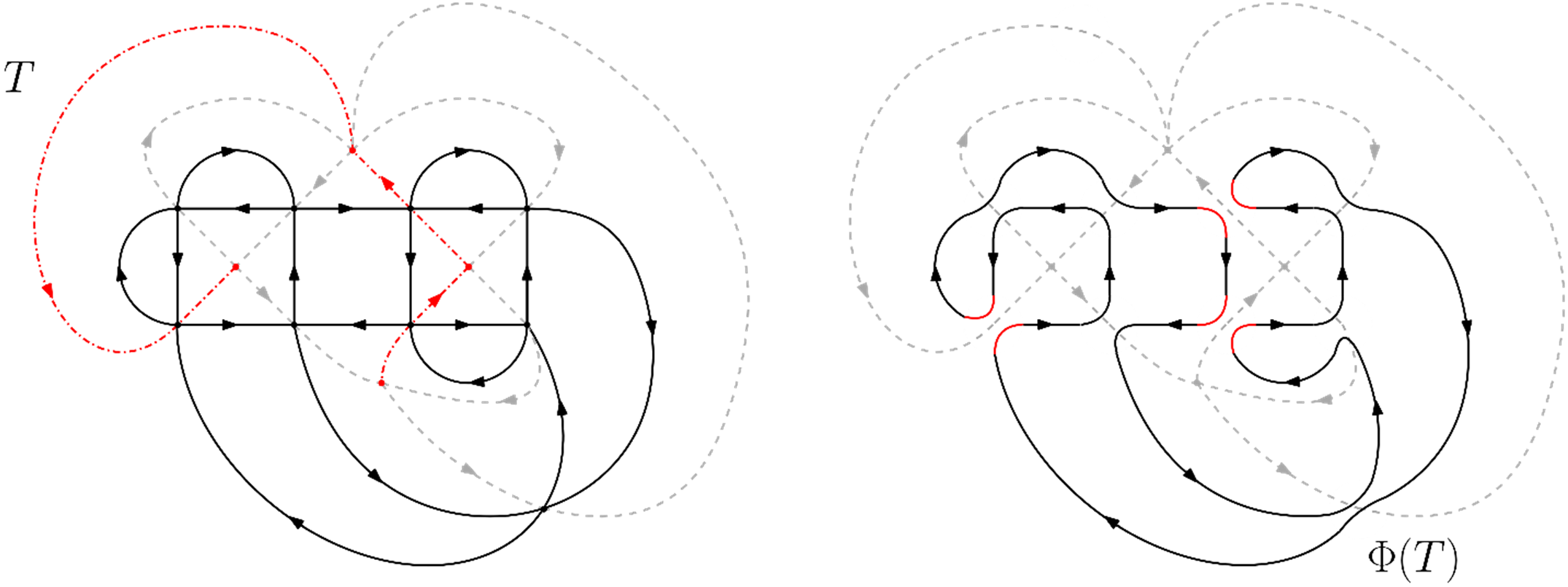
Figure 9. In the above image, $D$ is depicted in dashed grey, and $\overrightarrow{\mathcal{G}(L)}$ is depicted in black. On the left is a spanning tree $T$ of $D$. On the right is its image under $\Phi$.

Theorem 6.5.

Let $r\in\operatorname{V}(D)$ denote the vertex corresponding to the exterior region of $L$. Choose $v\in\operatorname{V}(\overrightarrow{\mathcal{G}(L)})$ such that $v=v_{e}$ for some $e\in E(D)$ with $\operatorname{fin}(e)=r$, and let $f_{v}\in\operatorname{E}(\overrightarrow{\mathcal{G}(L)})$ be the unique edge in the boundary of the exterior region such that $\operatorname{fin}(f_{v})=v$.

Then $F=\Psi_{v,f_{v}}\circ\Phi$ is a bijection between spanning trees of $D$ and arborescences of $\overrightarrow{\mathcal{G}(L)}$. Moreover, ${\rm wt}_{C}(A)={\rm wt}_{K}(T)t^{m_{2}-1}$ where $T\in\mathcal{T}(D)$, $A=F(T)\in\mathcal{A}_{v}(\overrightarrow{\mathcal{G}(L)})$, and $m_{2}$ is the number of blue regions, as defined above.

Figure 10 depicts an instance of the above bijection.

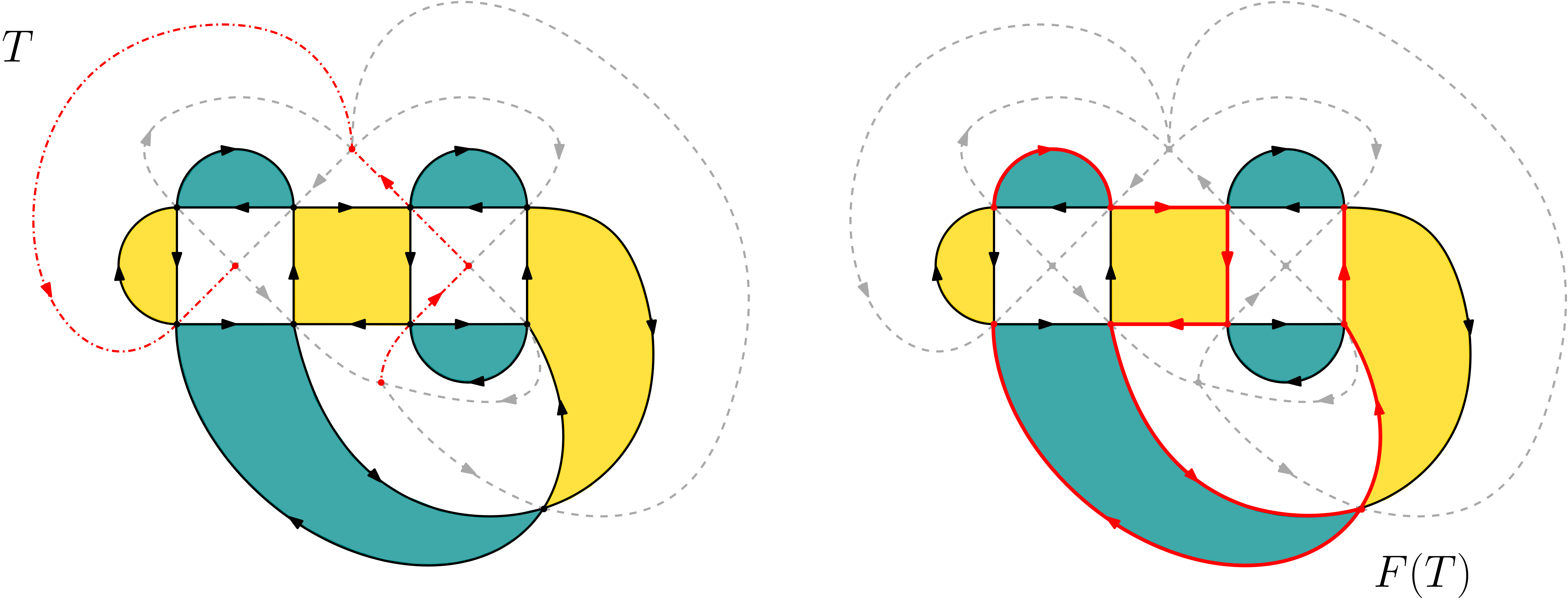
Figure 10. A spanning tree of $D$ and its image under $F$.

6.3. Proof of Theorem 6.5

To prove Theorem 6.5, we introduce two lemmas and accompanying notation.

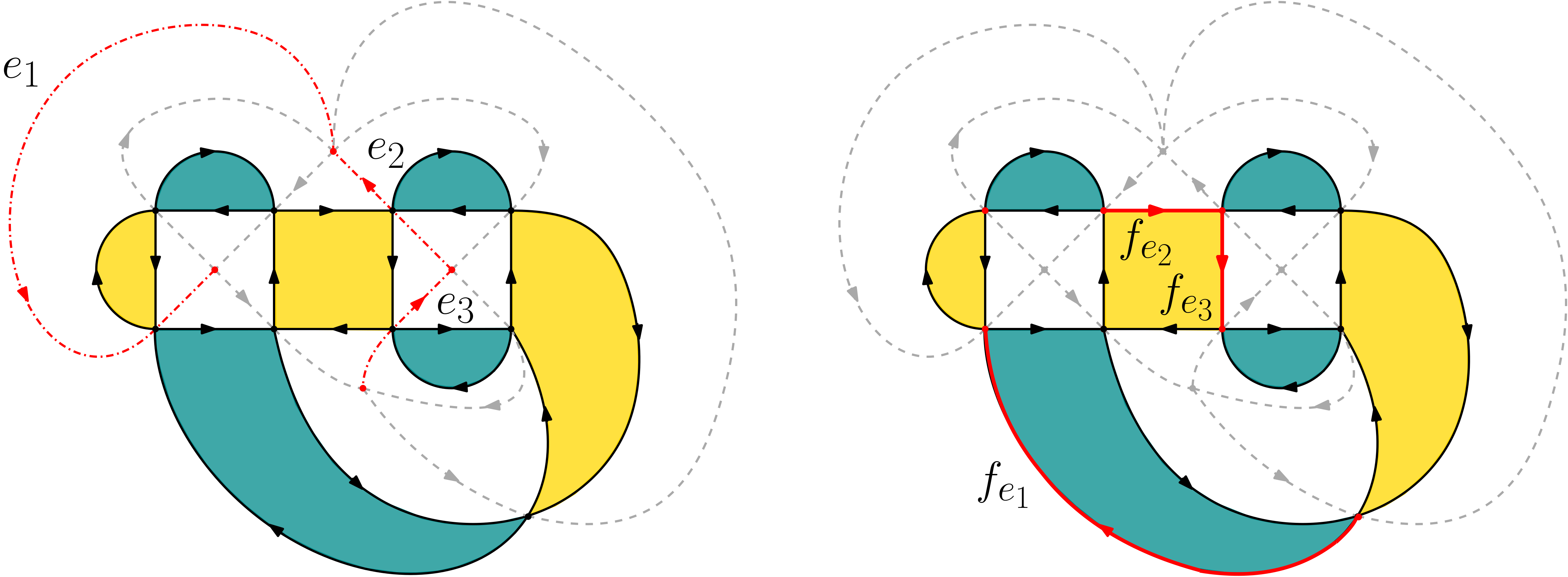
Figure 11. A spanning tree of $D$ and for each $e_{i}\in\operatorname{E}(T)$, the associated edge $f_{e_{i}}\in\operatorname{E}(F(T))$.

Definition 6.6.

Fix $T\in\mathcal{T}(D)$. For $e\in E(T)$ such that $v_{e}\neq v$, the root of $F(T)$, let $f_{e}\in\operatorname{E}(F(T))$ denote the unique edge of the arborescence $F(T)$ with final vertex $v_{e}$ (see Figure 11).

Lemma 6.7.

Fix a spanning tree $T$ of $D$, and let $r\in\operatorname{V}(D)$ denote the vertex corresponding to the exterior region of $L$. Fix $v\in\operatorname{V}(\overrightarrow{\mathcal{G}(L)})$ such that $v=v_{e}$ for some $e\in E(D)$ with $\operatorname{fin}(e)=r$. Let $f_{v}\in\operatorname{E}(\overrightarrow{\mathcal{G}(L)})$ be the unique edge in the boundary of the exterior region such that $\operatorname{fin}(f_{v})=v$. Then the edges in $\{f_{e}\ |\ e\in\operatorname{E}(T)\ \text{points towards}\ r\text{ in $T$}\}$ all border gold regions of $\overrightarrow{\mathcal{G}(L)}$, and the edges in $\{f_{e}\ |\ e\in\operatorname{E}(T)\ \text{points away from}\ r\text{ in $T$}\}$ all border blue regions of $\overrightarrow{\mathcal{G}(L)}$.

Proof.

For ease of reference, we say an edge of $\overrightarrow{\mathcal{G}(L)}$ is gold (resp. blue) if it borders a gold (resp. blue) region. Fix a spanning tree $T$ of $D$. We outline a procedure to determine the color of the first incoming edge to $v_{e}$ in $\Phi(T)$ for each $e\in\operatorname{E}(T)$. Note that the first incoming edge to $v_{e}$ in $\Phi(T)$ for each $e\in\operatorname{E}(T)$ is indeed $f_{e}$ according to Definitions 6.4 and 6.6.

Suppose first that $e\in\operatorname{E}(T)$ has $r$ as an endpoint. Let $P$ denote the portion of the oriented boundary of the exterior region of $\overrightarrow{\mathcal{G}(L)}$ from $v$ to $v_{e}$. We claim that the last edge of $P$ is the first edge incoming to $v_{e}$ along $\Phi(T)$ (which is $f_{e}$). Note that $\Phi(T)$, starting at $f_{v}$, can only leave the boundary of the exterior region when it meets a vertex of the form $v_{e^{\prime}}$ for some $e^{\prime}\in\operatorname{E}(T)$. Note also that upon leaving the boundary of the exterior region from a vertex of the form $v_{e^{\prime}}$ for some $e^{\prime}\in\operatorname{E}(T)$, the Eulerian cycle $\Phi(T)$ will return to $v_{e^{\prime}}$ before meeting any other vertex $v_{e^{\prime\prime}}$, $e^{\prime\prime}\in E(T)$, in the boundary of the exterior region. If the opposite were true, $T$ would contain a cycle, contradicting the fact that $T$ is a tree.

Accordingly, the first edge incident to $v_{e}$ along $\Phi(T)$ is blue if and only if the last edge of $P$ is blue. This happens if and only if $e$ is directed away from $r$ since the edges incident to $r$ alternate between incoming and outgoing (see the left and center images in Figure 12).

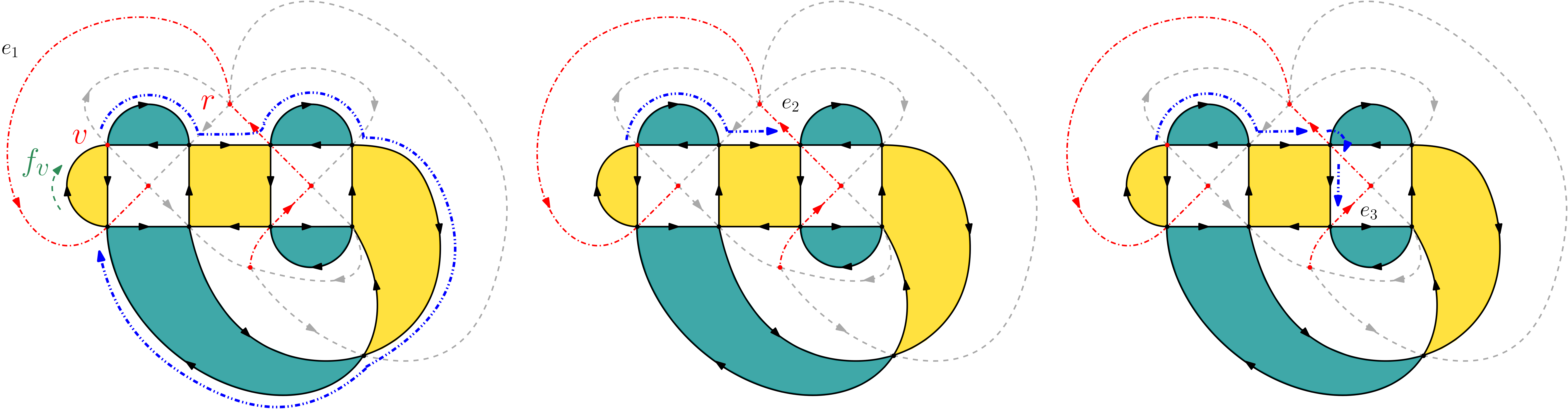
Figure 12. The procedure described in the proof of Lemma 6.7 to determine the first edge incident to $v_{e_{i}}$ for each of the edges of the spanning tree from Figures 10 and 11.

Next, we consider the case that $e\in\operatorname{E}(T)$ is not incident to $r$. Fix the shortest (undirected) path in $T$ from $r$ to a vertex of $e$, and let $e^{\prime\prime\prime}\neq e$ denote the final edge of this path. The edges $e$ and $e^{\prime\prime\prime}$ meet at a single vertex $w$. Let $P^{\prime}$ denote the oriented path from $v_{e^{\prime\prime\prime}}$ to $v_{e}$ in the boundary of the region of $\overrightarrow{\mathcal{G}(L)}$ corresponding to $w$ (in the rightmost image of Figure 12, $e$ is $e_{3}$, $e^{\prime\prime\prime}$ is $e_{2}$, and $w$ is the vertex where they meet). As before, the last edge of $P^{\prime}$ is the first edge incident to $v_{e}$ along $\Phi(T)$. If the length of the path connecting $v_{e^{\prime\prime\prime}}$ and $v_{e}$ is odd, then the colors of the first edges incident to $v_{e^{\prime\prime\prime}}$ and $v_{e}$ are identical, and $e^{\prime\prime\prime}$ and $e$ either both point towards $v$ or both point away from $v$. Similarly, if the length of the path connecting $v_{e^{\prime\prime\prime}}$ and $v_{e}$ is even, then the colors of the first edges incident to $v_{e^{\prime\prime\prime}}$ and $v_{e}$ are different, and exactly one of these edges points towards $v$. We, thus, achieve the desired result. ∎

Lemma 6.8.

Fix a spanning tree $T$ of $D$, and let $r\in\operatorname{V}(D)$ denote the exterior region of $L$. Fix $v\in\operatorname{V}(\overrightarrow{\mathcal{G}(L)})$ such that $v=v_{e}$ for some $e\in E(D)$ with $\operatorname{fin}(e)=r$. Let $f_{v}\in\operatorname{E}(\overrightarrow{\mathcal{G}(L)})$ be the unique edge in the boundary of the exterior region such that $\operatorname{fin}(f_{v})=v$. Let $f\in\operatorname{E}(\overrightarrow{\mathcal{G}(L)})$ be any edge bordering a blue region $C_{f}$ of $\overrightarrow{\mathcal{G}(L)}$. Then $f\in\operatorname{E}(F(T))$ if and only if

• $f$ is not the last edge in the boundary of $C_{f}$ to appear in the Eulerian tour $\Phi(T)$, and

• the final vertex $\operatorname{fin}(f)$ in $\overrightarrow{\mathcal{G}(L)}$ does not equal $v_{e}$ for some edge $e\in\operatorname{E}(T)$ directed towards the root $r$.

Proof.

First, suppose that $f$ is the last edge in the boundary of $C_{f}$ to appear in $\Phi(T)$. Then $f$ is first edge pointing into $\operatorname{fin}(f)$ in $\Phi(T)$ only when $\operatorname{fin}(f)=r$, so $f\notin\operatorname{E}(F(T))$.

If $\operatorname{fin}(f)=v_{e}$ where $e\in\operatorname{V}(T)$ is directed towards the root $r$, then by Lemma 6.7, $f_{e}$ must lie in the boundary of a gold region of $\overrightarrow{\mathcal{G}(L)}$. In particular, $f\neq f_{e}$, and so $f$ is not an edge of $F(T)$.

It now remains to show that all other edges $f$ which border a blue region of $\overrightarrow{\mathcal{G}(L)}$ must be in $F(T)$. Suppose $f$ satisfies conditions (a) and (b). One of the following cases must hold.

1. Case 1: The final vertex $\operatorname{fin}(f)=v_{e}$ for some edge $e\in\operatorname{E}(T)$ directed away from the root $r$. (Note that this implies $f\neq f_{v}$.)

   In this case, Lemma 6.7 implies that $f$ is an edge of $F(T)$.

2. Case 2: The final vertex $\operatorname{fin}(f)=v_{e}$ for some edge $e\in\operatorname{E}(D)$ which is not in $T$, and the unique edge $f^{\prime}$ in the boundary of $C_{f}$ with $\operatorname{fin}(f)=\operatorname{init}(f^{\prime})$ appears after $f$ in the Eulerian tour $\Phi(T)$.

   In this case, the only other edge of $\overrightarrow{\mathcal{G}(L)}$ with final vertex $\operatorname{fin}(f)$ must appear immediately before $f^{\prime}$ in $\Phi(T)$; therefore, $f$ is the first edge pointing into $\operatorname{fin}(f)$ in $\Phi(T)$. By the definition of $\Psi_{v,f_{v}}$, this implies $f$ is an edge of $F(T)$.

3. Case 3: The final vertex $\operatorname{fin}(f)=v_{e}$ for some edge $e\in\operatorname{E}(D)$ which is not in $T$, and the unique edge $f^{\prime}$ in the boundary of $C_{f}$ with $\operatorname{fin}(f)=\operatorname{init}(f^{\prime})$ appears before $f$ in the Eulerian tour $\Phi(T)$. We argue that this case would violate condition (a).

   Assuming Case 3, note that there must be a path $P$ in $\Phi(T)$ from $f^{\prime}$ to $f$, as shown below.

   Suppose that $g\in\operatorname{E}(\overrightarrow{\mathcal{G}(L)})$ is an edge not in $P$ such that $\operatorname{fin}(g)\in\operatorname{V}(P)$. Let $g^{\prime}$ be the edge immediately following $g$ in $\Phi(T)$; in particular, $\operatorname{init}(g^{\prime})=\operatorname{fin}(g)$. By construction of $\Phi$, $g$ and $g^{\prime}$ must either both lie inside the region bounded by $P$ or both lie outside it (see Definition 6.3). This implies that once $\Phi(T)$ reaches $f$, it cannot re-enter the portion of the graph enclosed by $P$. In particular, no edge in the boundary of $C_{f}$ can be reached after $f$ in $\Phi(T)$, so we have a contradiction with condition (a).

∎

Proof of Theorem 6.5. Let $w$ denote the degree of ${\rm wt}_{C}(F(T))$. For a region $R\in R(\overrightarrow{\mathcal{G}(L)})$, let $\partial R$ denote the oriented boundary of $R$ as a subgraph of $\overrightarrow{\mathcal{G}(L)}$.

$$w =\left|\{f\in\operatorname{E}(F(T))\ |\ f\ \text{is}\ \text{gold}\}\right|$$

$$=|\operatorname{E}(F(T))|-\left|\{f\in\operatorname{E}(F(T))\ |\ f\ \text{is}\ \text{blue}\}\right|$$

$$=(|V(\overrightarrow{\mathcal{G}(L)})|-1)-\left|\{f\in\operatorname{E}(F(T))\ |\ f\ \text{is}\ \text{blue}\}\right|.$$

Apply Lemma 6.8 to replace the second term in the difference above. Note that there are no edges of $\overrightarrow{\mathcal{G}(L)}$ which violate conditions $(a)$ and $(b)$ of the lemma simultaneously. Accordingly,

$$w =(|V(\overrightarrow{\mathcal{G}(L)})|-1)-\sum_{R\in R(\overrightarrow{\mathcal{G}(L)})\ \text{blue}}((|\operatorname{E}(\partial R)|-1)-\left|\{e\in\operatorname{E}(T)\ |\ v_{e}\in\partial R\ \text{and}\ e\ \text{points towards}\ r\}\right|)$$

$$=(|V(\overrightarrow{\mathcal{G}(L)})|-1)-\sum_{R\in R(\overrightarrow{\mathcal{G}(L)})\ \text{blue}}(|\operatorname{E}(\partial R)|-1)$$

$$\phantom{={}}+\sum_{R\in R(\overrightarrow{\mathcal{G}(L)})\ \text{blue}}\left|\{e\in\operatorname{E}(T)\ |\ v_{e}\in\partial R\ \text{and}\ e\ \text{points towards}\ r\}\right|$$

$$=(|V(\overrightarrow{\mathcal{G}(L)})|-1)-\left|\{e\in\operatorname{E}(\overrightarrow{\mathcal{G}(L)})\ |\ e\ \text{is blue}\}\right|+m_{2}+\left|\{e\in\operatorname{E}(T)\ |\ e\ \text{points towards}\ r\}\right|.$$

Now, the map $e\mapsto\operatorname{init}(e)$ is a bijection between blue edges of $\overrightarrow{\mathcal{G}(L)}$ and $\operatorname{V}(\overrightarrow{\mathcal{G}(L)})$, so

$$w=m_{2}-1+\left|\{e\in\operatorname{E}(F(T))\ |\ e\ \text{points towards}\ r\}\right|=m_{2}-1+|E(T)\backslash E_{\text{away}}(T)|.$$

Therefore, ${\rm wt}_{C}(A)={\rm wt}_{K}(T)t^{m_{2}-1}$. ∎

References

- [1] James W. Alexander, Topological invariants of knots and links, Trans. Amer. Math. Soc. 30 (1928), no. 2, 275–306.
- [2] John H. Conway, An enumeration of knots and links, and some of their algebraic properties, Computational problems in abstract algebra, Elsevier, 1970, pp. 329–358.
- [3] Richard H. Crowell, Genus of alternating link types, Ann. of Math. (2) 69 (1959), no. 2, 258–275.
- [4] Ralph Hartzler Fox, Some problems in knot theory, Topology of 3-manifolds and related topics (M.K. Fort, ed.), Prentice Hall, 1962, pp. 168–176.
- [5] Elena S. Hafner, Karola Mészáros, and Alexander Vidinas, Log-concavity of the Alexander polynomial, 2023, arXiv: 2303.04733.
- [6] Richard I. Hartley, On two-bridged knot polynomials, J. Aust. Math. Soc. 28 (1979), no. 2, 241–249.
- [7] In Dae Jong, Alexander polynomials of alternating knots of genus two, Osaka J. Math. 46 (2009), no. 1, 353–371.
- [8] András Juhász, Tamás Kálmán, and Jacob Rasmussen, Sutured Floer homology and hypergraphs, Math. Res. Lett. 19 (2012), no. 6, 1309–1328. MR 3091610
- [9] Tamás Kálmán and Hitoshi Murakami, Root polytopes, parking functions, and the HOMFLY polynomial, Quantum Topol. 8 (2017), no. 2, 205–248. MR 3659490
- [10] Tamás Kálmán and Alexander Postnikov, Root polytopes, Tutte polynomials, and a duality theorem for bipartite graphs, Proc. Lond. Math. Soc. 114 (2017), no. 3, 561–588.
- [11] Louis H. Kauffman, Formal knot theory, Dover books on mathematics, Dover Publications, 2006.
- [12] Nan Li and Alexander Postnikov, Slicing zonotopes. preprint, 2013.
- [13] Kunio Murasugi, On the Alexander polynomial of the alternating knot, Osaka Math. J. 10 (1958), no. 1, 181–189.
- [14] by same author, On the genus of the alternating knot II, Journal of the Mathematical Society of Japan 10 (1958), no. 3, 235–248.
- [15] by same author, On the Alexander polynomial of alternating algebraic knots, J. Aust. Math. Soc. 39 (1985), no. 3, 317–333.
- [16] Kunio Murasugi and Alexander Stoimenow, The Alexander polynomial of planar even valence graphs, Adv. in Appl. Math. 31 (2003), no. 2, 440–462. MR 2001624
- [17] Peter Ozsváth and Zoltán Szabó, Heegaard Floer homology and alternating knots, Geom. Topol. 7 (2003), 225–254.
- [18] Alexander Postnikov, Permutohedra, associahedra, and beyond, Int. Math. Res. Not. IMRN (2009), no. 6, 1026–1106.
- [19] Richard P. Stanley, Algebraic combinatorics, Springer, 2013.
- [20] Alexander Stoimenow, Newton-like polynomials of links, Enseign. Math. (2) 51 (2005), no. 3-4, 211–230.
- [21] Lilla Tóthmérész, A geometric proof for the root-independence of the greedoid polynomial of Eulerian branching greedoids, 2022, arXiv: 2204.12419.
- [22] William T. Tutte and Cedric A. B. Smith, On unicursal paths in a network of degree 4, Amer. Math. Monthly 48 (1941), no. 4, 233–237. MR 1525117
- [23] Tanja van Aardenne-Ehrenfest and Nicholas G. de Bruijn, Circuits and trees in oriented linear graphs, Simon Stevin 28 (1951), 203–217. MR 47311