Direct WIMP detection rates for transitions in isomeric nuclei

Abstract

The direct detection of dark matter constituents, in particular the weakly interacting massive particles (WIMPs), is central to particle physics and cosmology. In this paper we study WIMP induced transitions from isomeric nuclear states for two possible isomeric candidates: $\rm{}^{180}Ta$ and $\rm{}^{166}Ho$. The experimental setup, which can measure the possible decay of $\rm{}^{180}Ta$ induced by WIMPs, was proposed. The corresponding estimates of the half-life of $\rm{}^{180}Ta$ are given in the sense that the WIMP-nucleon interaction can be interpreted as ordinary radioactive decay.

I Introduction

At present there are plenty of evidences of dark matter from i) cosmological observations, the combined MAXIMA-1 [1], BOOMERANG  [2], DASI [3], COBE/DMR Cosmic Microwave Background (CMB) observations [4, 5], as well as the recent WMAP  [6] and Planck [7] data and ii) the observed rotational curves in the galactic halos, see e.g. the review [8]. It is, however, essential to directly detect such matter in order to unravel the nature of its constituents.

At the moment, there are many candidates, so-called Weakly Interacting Massive Particles (WIMPs), e.g. the LSP (Lightest Super-symmetric Particle) [9, 10, 11, 12, 13, 14, 15], technibaryon [16, 17], mirror matter [18, 19], Kaluza-Klein models with universal extra dimensions [20, 21] etc. Meanwhile, proposals such as dark matter as dark photons, axion-like particles and light scalar bosons were studied [22]. These models predict an interaction of dark matter with ordinary matter via the exchange of a scalar particle, which leads to a spin independent interaction (SI) or vector boson interaction, which leads to a spin dependent (SD) nucleon cross section. Additional theoretical tools are the structure of the nucleus, see e.g. [23, 24, 25, 26], and the nuclear matrix elements [27, 28, 29, 30, 31].

In this paper, we will focus on the spin dependent WIMP nucleus interaction. This cross section can be sizable in a variety of models, including the lightest super-symmetric particle (LSP) [32, 33, 29, 34], in the co-annihilation region [35], where the ratio of the SD to to the SI nucleon cross section, depending on $\tan{\beta}$ and the WIMP mass can be large, e.g. $10^{3}$ in the WIMP mass range 200-500 GeV.

Furthermore more recent calculations in the super-symmetric $SO(10)$ model [36], also in the co-annihilation region, predict ratios of the order of $2\cdot 10^{3}$ for a WIMP mass of about 850 GeV. Models of exotic WIMPs, like Kaluza-Klein models [20, 21] and Majorana particles with spin 3/2 [37], also can lead to large nucleon spin induced cross sections, which satisfy the relic abundance constraint. This interaction is very important because it can lead to inelastic WIMP-nucleus scattering with a non a prospect proposed some time ago [38] and considered in some detail by Ejiri and collaborators [39]. Indeed for a Maxwell-Boltzmann (M-B) velocity distribution the average kinetic energy of the WIMP is:

$$\langle T\rangle\approx 50\leavevmode\nobreak\ {\rm keV}\frac{m_{\chi}}{100\leavevmode\nobreak\ {\rm GeV}}$$ (1)

So, for sufficiently heavy WIMPs, the available energy via the high velocity tail of the M-B distribution may be adequate [40] to allow scattering to low lying excited states of of certain targets, e.g. of $57.7\leavevmode\nobreak\$keV for the $7/2^{+}$ excited state of ¹²⁷I, the 39.6 keV for the first excited $3/2^{+}$ of ¹²⁹Xe, 35.48 keV for the first excited $3/2^{+}$ state of ¹²⁵Te and 9.4 keV for the first excited $7/2^{+}$ state of ⁸³Kr. In fact calculations of the event rates for the inelastic WIMP-nucleus transitions involving the above systems have been performed [41, 42].

Interest in the inelastic WIMP-nucleus scattering has recently been revived by a new proposal to search for the de-excitation of meta-stable nuclear isomers [43] after such collisions. The longevity of these isomers is related to a strong suppression of $\gamma$ and $\beta$-transitions, typically inhibited by a large difference in the angular momentum for the nuclear transition. Collisional de-excitation by dark matter is possible since heavy dark matter particles can have a momentum exchange with the nucleus comparable to the inverse nuclear size, hence lifting tremendous angular momentum suppression of the nuclear transition.

II Kinematics

Evaluation of the differential rate for a WIMP induced transition $A^{i}_{iso}(E_{x})$ for an isomeric nuclear state at excitation energy $E_{x}$ to another one $A^{f}_{iso}(E^{\prime}_{x})$ (or to the ground state) proceeds in a fashion similar to that of the standard inelastic WIMP induced transition, except in the consideration of kinematics. We will make a judicious choice of the final nuclear state that can decay in a standard way to the ground state or to another lower excited state:

$$A^{i}_{iso}(E_{x})+\chi\rightarrow A^{f}_{iso}(E^{\prime}_{x})+\chi,$$ (2)

with $\chi$ the dark matter particle (WIMP). Assuming that all particles involved are non relativistic we get:

$$\frac{{\bf p}^{2}_{\chi}}{2m_{\chi}}+E_{x}=\frac{{\bf p}^{\prime 2}_{\chi}}{2m_{\chi}}+E^{\prime}_{x}+\frac{{\bf q}^{2}}{2m_{A}},$$ (3)

where ${\bf q}$ is the momentum transfer to the nucleus ${\bf q}={\bf p}_{\chi}-{\bf p}^{\prime}_{\chi}$ and $m_{A}$ is the isomer mass. So the above equation becomes

$$\frac{-{\bf q}^{2}}{2\mu_{r}}+\upsilon\xi q-\Delta=0,\quad\Delta=E_{x}-E^{\prime}_{x}\Leftrightarrow-\frac{m_{A}}{\mu_{r}}E_{R}+\upsilon\xi\sqrt{2m_{A}E_{R}}+\Delta=0,$$ (4)

where $\Delta>0$, $\xi$ is the cosine of the angle between the incident WIMP and the recoiling nucleus, $\upsilon$ the oncoming WIMP velocity, $\mu_{r}=\frac{m_{A}m_{\chi}}{m_{A}+m_{\chi}}$ the reduced mass of the WIMP-nucleus system and $E_{R}$ the nuclear recoil energy. From the above expression it is immediately apparent that

$$\xi=\frac{-\Delta+\frac{m_{A}}{\mu_{r}}E_{R}}{\upsilon\sqrt{2m_{A}E_{R}}}$$ (5)

Thus we find the next condition

$$-1\leq\frac{-\Delta+\frac{m_{A}}{\mu_{r}}E_{R}}{\upsilon\sqrt{2m_{A}E_{R}}}\leq 1$$

This means that for $-\Delta+\frac{m_{A}}{\mu_{r}}E_{R}>0$ the allowed range of velocities is

$$\upsilon_{2}\leq\upsilon\leq\upsilon_{\rm esc},\,\upsilon_{2}=\frac{-\Delta+\frac{m_{A}}{\mu_{r}}E_{R}}{\sqrt{2m_{A}E_{R}}},$$ (6)

where $\upsilon_{\rm esc}$ is the escape velocity, the maximum allowed velocity. For for $-\Delta+m_{A}/\mu_{r}\cdot E_{R}<0$ the allowed region is

$$\upsilon_{1}\leq\upsilon\leq\upsilon_{\rm esc},\,\upsilon_{1}=\frac{\Delta-\frac{m_{A}}{\mu_{r}}E_{R}}{\sqrt{2m_{A}E_{R}}}$$ (7)

At this point we should mention that in the standard inelastic scattering the region

$$\upsilon\leq\frac{E_{x}+\frac{m_{A}}{\mu_{r}}E_{R}}{\sqrt{2m_{A}E_{R}}}$$

is not available. Note the difference in sign between the previous equation and Eq.(6). As a result $\upsilon_{min}$ increases with $E_{x}$, which explains the suppression of the expected rates in the standard process as $E_{x}$ increases.

Based on Appendix A, in the special case of WIMP-nucleon scattering the maximum recoil energy is given by

$$\left(E_{R}\right)_{\rm max}=2m_{N}\upsilon_{\rm esc}^{2}\frac{1}{(1+x)^{2}}=2m_{N}\upsilon_{0}^{2}y_{\rm esc}^{2}\frac{1}{(1+x)^{2}},$$ (8)

where $x=m_{N}/m_{\chi}$. Using $\upsilon_{0}\approx 0.7\cdot 10^{-3}$ (in natural units) and $y_{\rm esc}=2.84$ we obtain

$$\left(E_{R}\right)_{\rm max}=8.0\times 10^{-6}m_{N}\frac{\rm GeV}{(1+x)^{2}}=8.0\frac{\rm keV}{(1+x)^{2}}$$ (9)

III Expressions for the cross section

The differential cross section is given by

$$d\sigma=\frac{1}{\upsilon}\frac{1}{(2\pi)^{2}}d^{3}{\bf q}\delta\left(\frac{q^{2}}{2\mu_{r}}-q\upsilon\xi-\Delta\right)\left(\frac{G_{F}}{\sqrt{2}}\right)^{2}|ME(q^{2})|^{2}$$ (10)

where $|ME(q)|^{2}$ is the nuclear matrix element of the WIMP-nucleon interaction in dimensionless units and $G_{F}$ the standard weak interaction strength. Integrating over $\xi$ by making use of the $\delta$ function we get

$$d\sigma=\frac{1}{\upsilon}\frac{1}{(2\pi)^{2}}q^{2}dq\frac{2\pi}{q\upsilon}\left(\frac{G_{F}}{\sqrt{2}}\right)^{2}|ME(q^{2})|^{2}$$ (11)

III.1 The elementary nucleon cross section

New physics is contained in elementary nucleon interaction, so we prefer to parameterize in terms of the elementary nucleon cross section. In the case of the nucleon Eq.(11) becomes

$$d\sigma=\frac{1}{\upsilon^{2}}\frac{1}{2\pi}qdq\left(\frac{G_{F}}{\sqrt{2}}\right)^{2}|ME_{N}|^{2}=\frac{1}{\upsilon^{2}}\frac{1}{2\pi}m_{N}dE_{R}\left(\frac{G_{F}}{\sqrt{2}}\right)^{2}|ME_{N}|^{2}$$ (12)

Folding the last equation with the velocity distribution and integrating over the allowed recoil energies (see the Appendix C), we obtain

$$\sigma_{N}=4.0\frac{1}{2\pi}m^{2}_{N}\left(\frac{G_{F}}{\sqrt{2}}\right)^{2}\left(f_{V}^{2}+3f_{A}^{2}\right)$$ (13)

IV Nuclear structure

The microscopic structure of atomic nuclei is described in terms of the spherical shell model [44, 45, 46], introduced in 1949 in order to explain the magic numbers 2, 8, 20, 28, 50, 82, 126, …, at which nuclei present particularly stable configurations. The shell model is obtained from the three-dimensional isotropic harmonic oscillator, to which the spin-orbit interaction is added. It offers a satisfactory description of nuclei with few valence protons and valence neutrons outside closed shells, corresponding to the magic numbers, but it fails to explain the experimentally observed large nuclear quadrupole moments away from closed shells, where it has been suggested [47] in 1950 that spheroidal instead of spherical shapes lead to greater stability. Along this line, the collective model of Bohr and Mottelson [48, 49] was introduced in 1952, in which departure from the spherical shape and from axial symmetry are described by the collective variables $\beta$ and $\gamma$, respectively. Furthermore in 1955 the Nilsson model [50, 51, 52] was introduced, in which a cylindrical harmonic oscillator is used instead of a spherical one, characterized by a deformation $\epsilon$, reflecting the departure of the cylindrical shape from spherical one. The single particle orbitals in the Nilsson model are labeled by $\Omega[Nn_{z}\Lambda]$, where $N$ is the total number of the oscillator quanta, $n_{z}$ is the number of quanta along the $z$-axis of cylindrical symmetry, while $\Lambda$ ($\Omega$) is the projection of the orbital (total) angular momentum on the $z$-axis.

In what follows it will be of interest to consider the expansions of the Nilsson orbitals in the spherical shell model basis $|Nlj\Omega\rangle$, where $N$ is the principal quantum number, $l$ ($j$) is the orbital (total) angular momentum, and $\Omega$ is the projection of the total angular momentum on the $z$-axis. The necessary expansions have been obtained as described in [53] and are shown in Tab. 3 and 4 for three different values of the deformation $\epsilon$.

An important remark on the expansions shown in Table 3 is in order. One can see that there is a basic difference between intruder orbitals (orbitals pushed within the spherical shell model by the spin-orbit interaction to the oscillator shell below) and normal parity orbitals (orbitals remaining in their own oscillator shell). Intruder orbitals remain concentrated on one spherical shell model vector at all deformations, while normal parity orbitals are concentrated on one spherical shell model orbital at small deformation, but will in general be distributed onto several spherical shell model orbitals at large deformations. The implications of this difference will become clear below. It should be mentioned that the “purity” observed in the case of the intruder orbitals is due to the fact that they do not mix with their normal parity neighbors, while the normal parity orbitals, of which there are more than one, do mix among themselves.

IV.1 The nucleus ¹⁶⁶Ho

The even-even core of $\rm{}^{166}_{\leavevmode\nobreak\ 67}Ho_{99}$ is $\rm{}^{164}_{\leavevmode\nobreak\ 66}Dy_{98}$, for which the experimental value of the collective deformation variable $\beta$ is 0.3486 [54], thus the Nilsson deformation $\epsilon=0.95\beta$ [52] is 0.3312 .

Covariant density functional theory calculations using the DDME2 functional indicate that the first neutron orbitals lying above the Fermi surface of the core nucleus $\rm{}^{164}_{\leavevmode\nobreak\ 66}Dy_{98}$ are 1/2[521] (lower) and 7/2[633] (higher), while the first proton orbitals lying above the Fermi surface of the core nucleus $\rm{}^{164}_{\leavevmode\nobreak\ 66}Dy_{98}$ are 7/2[523] (lower) and 7/2[404] (higher), with 3/2[411] lying at the Fermi surface.

In 1978 it has been argued that the $0^{-}$ ground state of $\rm{}^{166}_{\leavevmode\nobreak\ 67}Ho_{99}$ should arise from the coupling of the 7/2[633] neutron to the 7/2[523] proton. The $7^{-}$ isomer state can also arise from these orbitals.

Let us now consider the formation of the above mentioned states under the light of the expansions of the Nilsson orbitals in terms of spherical shell model orbitals, shown in Tabs. 3 and 4. Both the proton 7/2[523] and neutron 7/2[633] orbitals are intruder ones, therefore they are mainly concentrated on the spherical shell model vectors $|5\ 5\ 11/2\ 7/2\rangle$ and $|6\ 6\ 13/2\ 7/2\rangle$ respectively, although other vectors with smaller coefficients also contribute, as seen in Tab. 3 and 4.

IV.2 The nucleus ¹⁸⁰Ta

The even-even core of ${}^{180}_{\leavevmode\nobreak\ 73}$Ta₁₀₇ is ${}^{178}_{\leavevmode\nobreak\ 72}$Hf₁₀₆, for which the experimental value of the collective deformation variable $\beta$ is 0.2779 [54], thus the Nilsson deformation $\epsilon=0.95\beta$ [52] is 0.2640 .

Several different theoretical calculations, including covariant density functional theory using the DDME2 functional [55, 56], Skyrmre-Hartree-Fock-BCS [57], as well as a two quasi-particle plus rotor model in the mean field represented by a deformed Woods-Saxon potential [58] agree that the first neutron orbital lying above the Fermi surface of the core nucleus $\rm{}^{178}_{\leavevmode\nobreak\ 72}Hf_{106}$ is the 9/2[624] orbital, while the first proton orbital lying above the Fermi surface of the core nucleus $\rm{}^{178}_{\leavevmode\nobreak\ 72}Hf_{106}$ is the 9/2[514] orbital. Therefore it is safe to assume that these two orbitals will play a major role in the formation of the $9^{-}$ isomer state of $\rm{}^{180}_{\leavevmode\nobreak\ 73}Ta$.

The question then comes from which orbitals the excited state $2^{+}$ may arise. The above mentioned covariant density functional theory using the DDME2 functional [55, 56], calculations and Skyrmre-Hartree-Fock-BCS [57] calculations indicate that the last neutron orbital below the Fermi surface is the 5/2[512] orbital, while the last proton orbital below the Fermi surface is the 7/2[404] orbital. Then it is plausible that the $2^{+}$ excited state will come from combining the proton 9/2[514] orbital (the first orbital above the Fermi surface) with the neutron 5/2[512] orbital (the first orbital below the Fermi surface).

It is instructive to consider the formation of the aforementioned states under the light of the expansions of the Nilsson orbitals in terms of spherical shell model orbitals, shown in Tab. 3 and 4 The orbitals participating in the formation of the $9^{-}$ isomer, proton 9/2[514] and neutron 9/2[624], are both intruder orbitals, thus the main contribution comes from the $|5\ 5\ 11/2\ 9/2\rangle$ component of the former and the $|6\ 6\ 13/2\ 9/2\rangle$ component of the latter. The orbitals participating in the formation of the $2^{+}$ excited state are the proton 9/2[514] (intruder) and neutron 5/2[512] (normal parity) orbitals, from which the leading contribution will come from the $|5\ 5\ 11/2\ 9/2\rangle$ and $|5\ 3\ 7/2\ 5/2\rangle$ vectors respectively.

V Considerations of the $\rm{}^{166}Ho$ target

So we will begin with the nucleus ¹⁶⁶Ho, which is well studied, see, e.g., [59]. This is an odd-odd nucleus (Z=67, N=99), which is a deformed nucleus described in the Nilsson model by $\left(\frac{7}{2}\right)^{-}[523]$ for protons, deformed level associated with the spherical $0h$ level, and the $\left(\frac{7}{2}\right)^{+}[633]$ associated with the spherical level $0i$ for neutrons. It is convenient to express these states in a spherical basis in terms of a deformation [60]. Thus for the purpose of our calculation it is sufficient to consider the expression

$$\left(\frac{7}{2}\right)^{-}[523]\leftrightarrow C_{0h_{11/2}}|0h_{11/2}\rangle,\,\left(\frac{7}{2}\right)^{+}[633]\leftrightarrow C_{0i_{11/2}}|0i_{11/2}\rangle+C_{0i_{13/2}}|0i_{13/2}\rangle$$ (14)

with

$$C_{0h_{11/2}}=0.9836,\,C_{0i_{11/2}}=-0.1,C_{0i_{13/2}}=0.9658$$ (15)

It is reasonable to assume that this odd-odd nucleus can be considered as a two particle system composed of one proton and one neutron in the above levels. Thus we get

$$\begin{split}0^{-}&=C_{0i_{11/2}}C_{0h_{11/2}}\left[|0i_{11/2}\otimes 0h_{11/2}\rangle\right]^{0},\\ 7^{-}&=C_{0h_{11/2}}\left(C_{0i_{11/2}}\left[|0i_{11/2}\otimes 0h_{11/2}\rangle\right]^{7}+|C_{0i_{13/2}}\left[|0i_{13/2}\otimes 0h_{11/2}\rangle\right]^{7}\right)\end{split}$$ (16)

V.1 The nuclear matrix elements

In spite of the fact that the coefficient $C_{0i_{11/2}}$ is small, the inclusion of the $0i_{11/2}$ is mandatory to make the $0^{-}$ ground state wave function. The inclusion of the $0i_{13/2}$ state with the large coupling is helpful but it can not lead to proton induced transitions. So one expects a suppression of nuclear matrix element. The operator for the transition has the structure $T^{\lambda,J}$ with rank $J=7$ and orbital rank $\lambda=J-1,J,J+1$. The interaction cannot convert protons to neutrons or vice versa. So the $\lambda=J=7$ is excluded by parity conservation. Thus $\lambda=J=6,8$, i.e. only the spin induced transitions are allowed. As a result in this case the ratio of the nuclear matrix element divided by the corresponding one for the nucleon can be cast in the form:

$$R_{ME(q^{2})}^{2}=\frac{|ME(q^{2})|^{2}_{nuc}}{|ME_{N}|^{2}}=C_{VA}\left(R_{ME(q^{2})}^{2}\right)_{0},\,C_{VA}=\frac{f_{A}^{2}}{f_{V}^{2}+3f_{A}^{2}}$$ (17)

The function $R_{ME(q^{2})}^{2}$ is independent of the scale, but it does depend on the ratio $f_{A}/f_{V}$ via the coefficient

$$C_{VA}=\left\{\begin{array}[]{cc}\leavevmode\nobreak\ \leavevmode\nobreak\ 0,&f_{V}>>fA\\ 1/3,&f_{V}<<fA\\ 1/4,&f_{V}\approx fA\\ \end{array}\right.$$ (18)

The vector current does not contribute in this case, but the first line in this expression comes from the explicit dependence of the cross section on the couplings (see Eq.(45)). In evaluating the nuclear matrix elements one needs the reduced matrix element

$$RME=\langle 0^{6}||T^{\lambda,J}||7^{-}\rangle$$

Using standard Racah techniques [61] one can obtain Eq.(63) of the Appendix D. A detailed explicit calculation reduced matrix elements in the case of $\rm{}^{166}Ho$ is given in section D.1.

After that one can incorporate into the reduced matrix element the form factor associated with in each orbit, obtained via the corresponding radial integrals of the spherical Bessel $j_{\lambda}(qr)$ finding this way the single particle form factor for each orbit, see Appendix E.

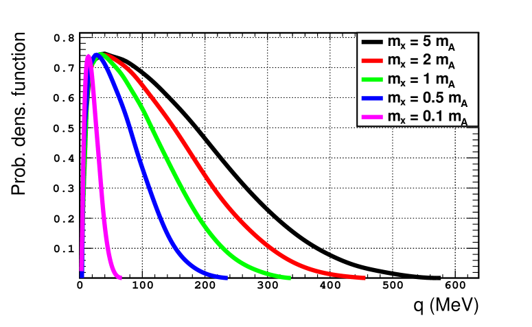
Figure 16: The allowed momentum distribution (defined in Appendix B) arising from the maximum allowed velocity (escape velocity) of the distribution for $\rm{}^{166}Ho$. Different line colors correspond to the WIMP masses $m_{\chi}=(0.1,\,0.5,\,1,\,2,\,5)m_{A}$

Let us now consider the allowed range of the momentum transfer. As we can see the minimum velocity must be smaller than the escape velocity, see Eq.38. For a M-B distribution see Eq.(43) with $y_{i}=\upsilon_{i}/\upsilon_{0},\leavevmode\nobreak\ i=1,2$. This momentum dependence is exhibited in Fig. 16. The nuclear matrix element $\left(R_{ME(q^{2})}^{2}\right)_{0}$ is exhibited in Fig. 4. We observe that it is greatly suppressed. This may be surprising in view of the fact that all single particle form factors involved are much larger, see Fig. 1 and take its square. These form factors, however, are much smaller the nuclear form factors encountered in the case of the standard WIMP searches involving the elastic WIMP-nucleus scattering, see Fig . 2.

This suppression appears to be mainly due to the geometric factors involved in the reduced matrix elements, i.e. nine-j symbols, Racah functions etc as well as due to smallness of the coefficient $C{i_{11/2}}$. Indeed the total nuclear matrix element can be written as

$$NME_{t}=\sum_{\ell,\lambda}C_{\ell,\lambda}FF_{\ell,\lambda}(q)$$

From the above reduced ME we find

$$C_{0i,8}=0.0203,\,C{{}_{0}i,6}=-0.01935,\,C_{0f,8}=0.000737,\,C_{0f,6}=0.00374.$$ (19)

The corresponding shell model single particle form factors are exhibited in Fig.  1. There appears to be some cancellation due to their size, but it is mainly a consequence of the fact that all the coefficients $C_{\ell,\lambda}$ are small and not of the same sign. Furthermore recall that, after incorporating the statistical factor

$$\left(R_{ME(q^{2})}^{2}\right)_{0}=\frac{1}{15}(NME_{t})^{2}$$

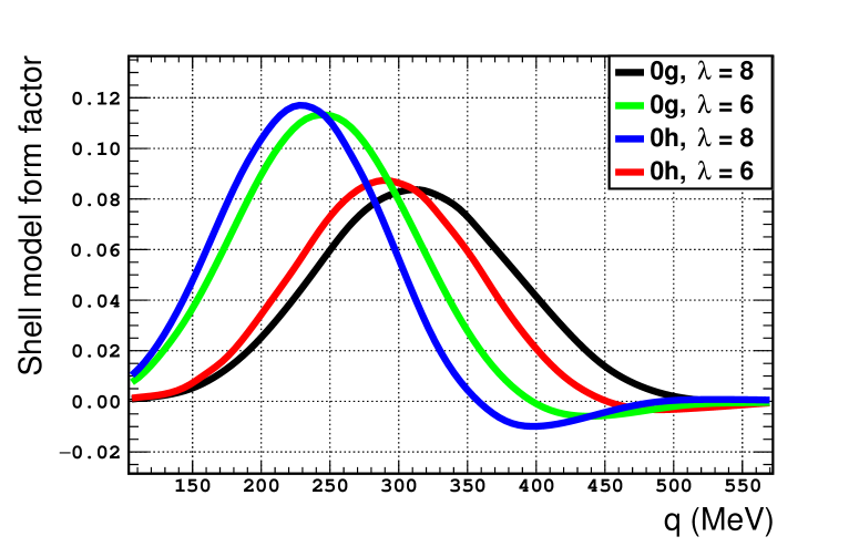
Figure 1: The shell model single particle form factors encountered in the case of a WIMP induced nuclear transition with $\Delta J=7$ for ¹⁶⁶Ho, with $\lambda$ is the orbital rank of the operator (multi-polarity).

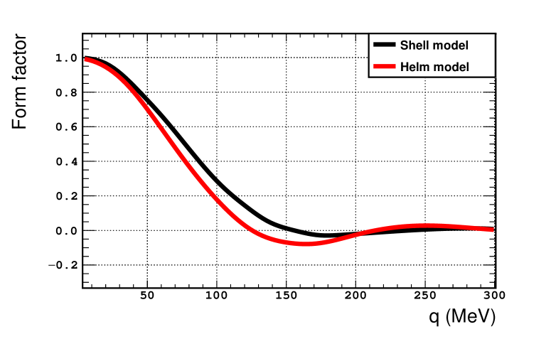
Figure 2: The shell model form factor encountered in the case of a WIMP induced elastic nuclear transition for ¹⁶⁶Ho and the same with the Helm form factor. The nuclear Matrix element in this case is obtained by multiplying this form factor with the number of nucleons in the nucleus, here $A=166$.

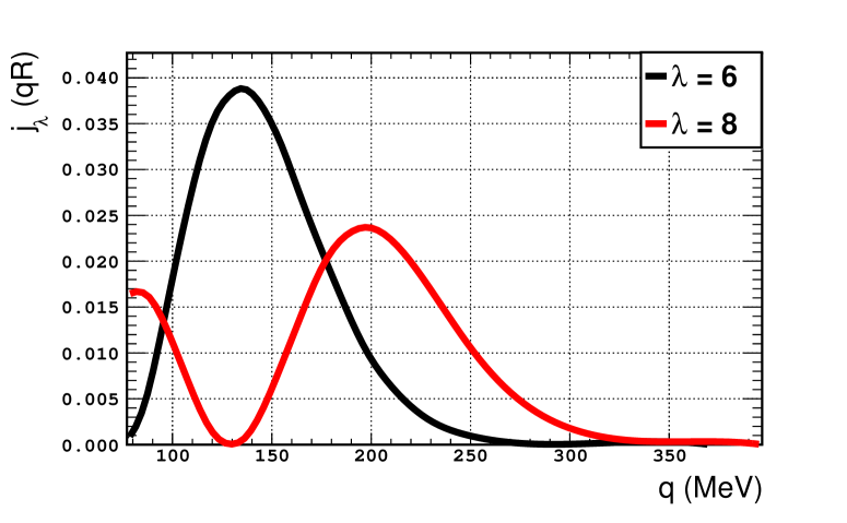
Figure 17: The function $j_{\lambda}(qR)$ for an A=156 nucleus in the range of $q$ of interest in the present work, $\lambda=8$ red line and $\lambda=6$ black line.

In addition it is also likely that the single particle form factors in the shell model are suppressed, or at least much smaller than implied by the scale set by the spherical Bessel functions $j_{\lambda}$, see Fig. 17. This suppression is not very significant, but ideally all fours single particle form factors could be determined experimentally.

For orientation purposes we will consider Helm like single particle form factors:

$$F_{\lambda}(q)=(2\lambda+1)e^{-\frac{1}{2}a^{2}q^{2}}\frac{j_{\lambda}(qR)}{qR}$$ (20)

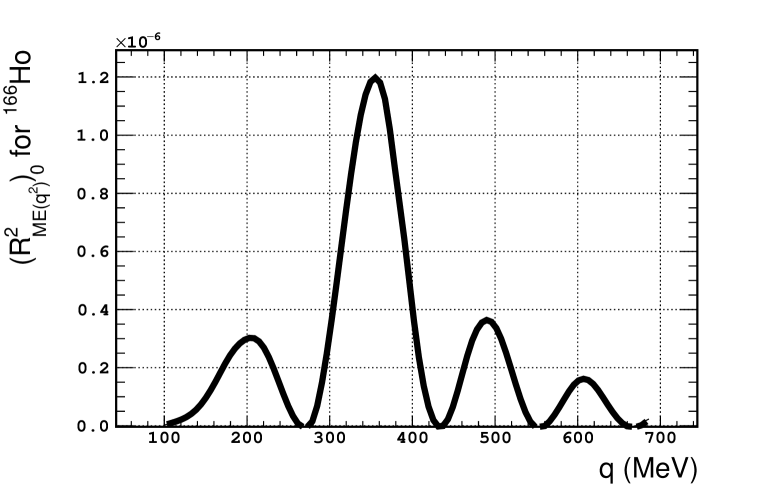
Figure 18: The same as in Fig. 4 obtained with Helm type single particle form factors. The restrictions on the allowed momenta are the same as in Fig. 4.

This is an extension of the Helm-form factor [62], normalized so that it is unity for $\lambda=1$ at $q=0$. This expression for $a=0.6$F and $R=6.87$F is exhibited in Fig. 3. The nuclear matrix element using these form factors is exhibited in Fig. 18.

There is now an improvement of two orders of magnitude, but the obtained result is still quite small.

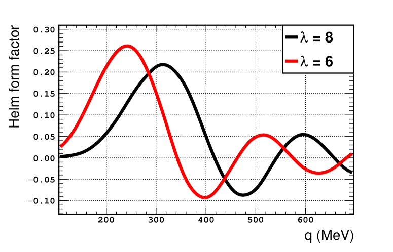
Figure 3: The Helm form factors $FFH_{\lambda}(q)$ for $\lambda=6$, red line, and for $\lambda=8$, black line, in the case of ¹⁶⁶Ho and momentum transfer of interest in the present work.

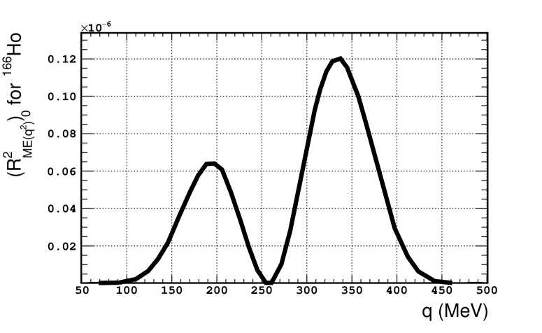
Figure 4: The function $\left(R_{ME(q^{2})}^{2}\right)_{0}$ for ¹⁶⁶Ho, which essentially is the ratio of the nuclear matrix element divided by the corresponding one for the nucleon, with the factor $\frac{f_{A}^{2}}{3f_{A}^{2}+f_{V}^{2}}$ removed. The part of the space above $q_{\rm max}=(65.6,233,349,464,579$ is not allowed for the case of $m_{\chi}=(0.1,\,0.5,\,1,\,2,\,5)m_{A}$ respectively (see Fig. 16 and the text for details).

In the case of the Helm-like form factors proceeding as in the case of shell model one finds

$$RME(q)=\sum_{\lambda}C_{\lambda}FFH_{\lambda}(q)$$ (21)

with

$$C_{\lambda}={0.02107,-0.01561}$$ (22)

These coefficients are also small. The negative sign in Eqs.(19) and (22) leads to suppression of the nuclear matrix element.

V.2 Some results for ¹⁶⁶Ho

The numerical value of

$$\Lambda\frac{m_{A}}{m_{N}^{2}}\frac{1}{\upsilon^{2}_{0}}\frac{1}{2\pi}$$

in Eq.45 using Eq. (17) with $f_{A}/f_{V}=1$, is 0.063 for A=166, expressed in units of keV^-1. The plot for $\frac{1}{\upsilon_{0}}\frac{1}{\sigma_{N}}\Big{\langle}\upsilon\frac{d\sigma}{dE_{R}}\Big{\rangle}$ versus the previous one multiplied with $0.063$. We prefer to express it as a function of $E_{R}$ in units of keV, i.e Fig. 5.

The expressions for $\sigma_{N}$, $\phi$ and $R$ can be obtained using the relevant values for the nucleon:

$$\sigma_{N}=3.5\cdot 10^{-39}(f_{V}^{2}+3f_{A}^{2}),{\rm\qquad cm^{2}}$$

$$\Phi=2.1\cdot 10^{38}\frac{m_{N}}{m_{\chi}},\qquad{\rm cm^{-2}y^{-1}}$$

(kinematics factor), yielding (see the Appendix C):

$$R_{N}=\Phi\sigma_{N}N_{N}=0.72\cdot(f_{V}^{2}+3f_{A}^{2}),\qquad{\rm y^{-1}}$$

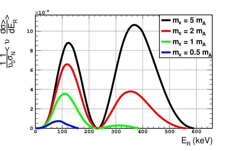
Figure 5: The function $\frac{1}{\upsilon_{0}}\frac{1}{\sigma_{N}}\langle\upsilon\frac{d\sigma>}{dE_{R}}\rangle$ in units of keV^-1. The Helm type form factor has been employed.

The same result holds for the obtained differential rate

$$\frac{1}{R_{N}(m_{\chi})}\frac{dR}{dE_{R}}$$

since the WIMP density used in obtaining the densities is the same. The situation is, however, different if one is comparing the obtained differential rate relative to the total rate for the nucleon at some fixed value of the WIMP mass. Indeed the obtained differential rate in units total rate of the nucleon for $m_{N}/m_{\chi}=1$ is exhibited in Fig. 6. The exhibited differential rate contains, of course, the WIMP mass dependence arising from the WIMP density in our galaxy.

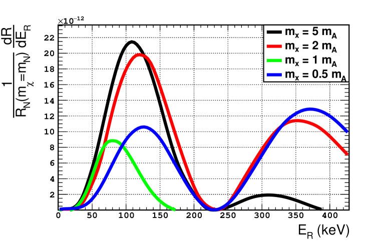
Figure 6: The differential rate relative to the total nucleon rate (for $m_{\chi}=m_{N}$), $\frac{1}{R_{N}(m_{\chi}=m_{N})}\frac{dR}{dE_{R}}$, in units of keV^-1. The Helm type form factor has been employed. It also contains the WIMP mass dependence arising from the WIMP density in our galaxy.

With such results the WIMP detection with the $\rm{}^{166}Ho$ appears very problematic.

VI Considerations of the $\rm{}^{180}Ta$ target

We begin by considering the transition of the isomeric $9^{-}$ state to the $2^{+}$ state. The momentum dependence of the cross section arising from the velocity distribution is different from that of $\rm{}^{166}Ho$, since the transition energy is $\Delta=37$ keV. Thus the analog of Fig.  16 is given in Fig. 7.

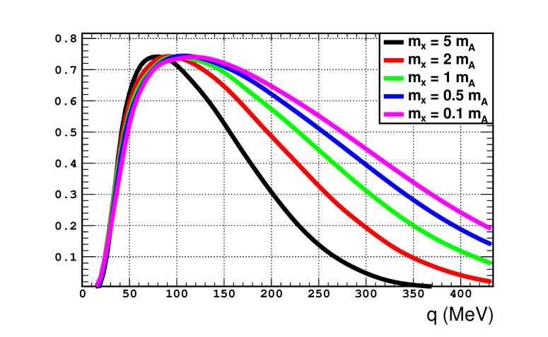
Figure 7: The allowed momentum distribution (defined in Appendix B) arising from the maximum allowed velocity (escape velocity) of the distribution, in the case of $\rm{}^{180}Ta$. For different WIMP masses $m_{\chi}=(0.1,\,0.5,\,1,\,2,\,5)m_{A}$. The transition energy is $\Delta=37$ keV.

To proceed further we need to determine the structure of the target $\rm{}^{180}Ta$. As explained in section IV.2 in the context of the Nilsson model we can consider the proton orbital $\frac{9}{2}$[514] both in the initial state $9^{-}$ and the final $2^{+}$. Furthermore for the neutrons we use $\frac{9}{2}$[624] for the $9^{-}$ and the $\frac{5}{2}$[512] for the $2^{+}$. To proceed further we use the expansion of the Nilsson orbitals into shell model states found in Tables 3 and 4 for deformation parameter 0.30. Note that in this case only the neutrons can undergo transitions, while the protons are just spectators. In the case of the shell model one encounters 8 transition types with odd multi-polarities.

VI.1 Shell model form factors

The vector and axial vector reduced nuclear matrix elements can be obtained using Eq.(62) where the quantities with subscript 1 indicate neutrons and those with 2 are associated with protons. Thus we find:

$$RME_{V}=\frac{f_{V}}{f_{A}}(0.0644445F(4,3,7,u)+1.01419F(4,5,7,u)+1.01419F(4,5,9,u)+1.52946F(6,3,7,u)+$$

$$1.52946F(6,3,9,u)+1.52946F(6,5,7,u)+1.79799F(6,5,9,u)+2.19718F(6,5,11,u))$$

$$RME_{A}=0.321503F(4,3,7,u)+2.05117F(4,5,7,u)+2.16715F(4,5,9,u)+2.04512F(6,3,7,u)+3.3217$$

$$F(6,3,9,u)+2.04512F(6,5,7,u)+2.31181F(6,5,9,u)+3.58938F(6,5,11,u)$$

In the above expressions $F(\ell,\ell^{\prime},\lambda)$ are the single particle form factors. The first two integers indicate orbital angular momentum quantum numbers $\ell,\ell^{\prime}$, while the last integer $\lambda$ gives the multipolarity of the transition. The quantity $u$ corresponds to $b_{N}q$, where $b_{N}$ is the harmonic oscillator length parameter. The nuclear matrix elements have been normalized as above in the case $\rm{}^{166}Ho$, see Eq.(17), with a compensating factor of $f_{A}$ appearing explicitly in the cross-section, Eq.45. The relevant form factors are exhibited in Fig. 8.

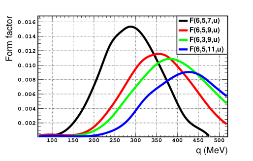
(a)

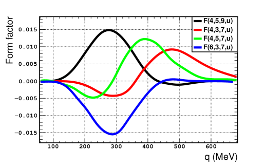
(b)

Figure 8: (a)The form factors for F(6,5,7,u), F(6,5,9,u), F(6,5,11,u) and F(6,3,9,u) are exhibited (b) The form factors F(6,3,7,u), F(4,5,7,u), F(4,5,9,u) and F(4,3,7,u) are shown.

The relevant nuclear ME is given by:

$$R^{2}_{ME}(q^{2})=\frac{1}{19}\left(RME_{V}^{2}+RME_{A}^{2}\right)$$ (23)

Its momentum dependence is exhibited in Fig.  9. We should note that the large value of the matrix element in the case of large $f_{V}$ is due to the normalization adopted to make the matrix element independent of the scale. Recall that the corresponding factor appears in the cross section. In the present work we will adopt $f_{V}=f_{A}$.

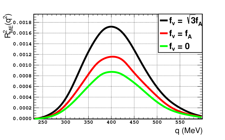
Figure 9: The momentum dependence of the expression $R^{2}_{ME}(q^{2})$ is exhibited as a function of $q$ for different values of $f_{V}$.

VI.2 Phenomenological form factors

It is generally believed that the shell model single particle factors lead to large suppression, so phenomenological form factors may be preferred. One example is the the Helm form factor, see Eq.(20). This has already been employed in the case of even transitions. We will employ here for odd (parity changing) transitions. Our treatment means that the radial integrals are independent of the angular momentum quantum numbers $\ell,\leavevmode\nobreak\ \ell^{\prime}$. The obtained results are exhibited in Fig. 10.

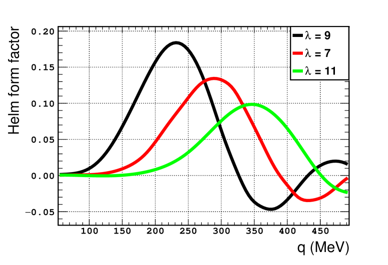
Figure 10: The Helm type form factors for $\lambda=7$, $\lambda=9$ and $\lambda=11$.

The reduced matrix elements for the vector and the axial vector are:

$$\begin{split}RMEH_{A}&=3.58938F_{11}(a,q,R)+6.46292F_{7}+7.80066F_{9}(a,q,R)\\ RMEH_{V}&=\frac{f_{V}}{f_{A}}(2.19718F_{11}(a,q,R)+4.13756F_{7}(a,q,R)+4.34165F_{9}(a,q,R)),\end{split}$$ (24)

where $F_{\lambda}$ are the Helm single particle form factors. The nuclear matrix element is:

$$R^{2}_{MEH}(q^{2})=\frac{1}{19}\left(RMEH_{V}^{2}+RMEH_{A}^{2}\right)$$ (25)

The momentum dependence of this ME is exhibited in Fig. 11

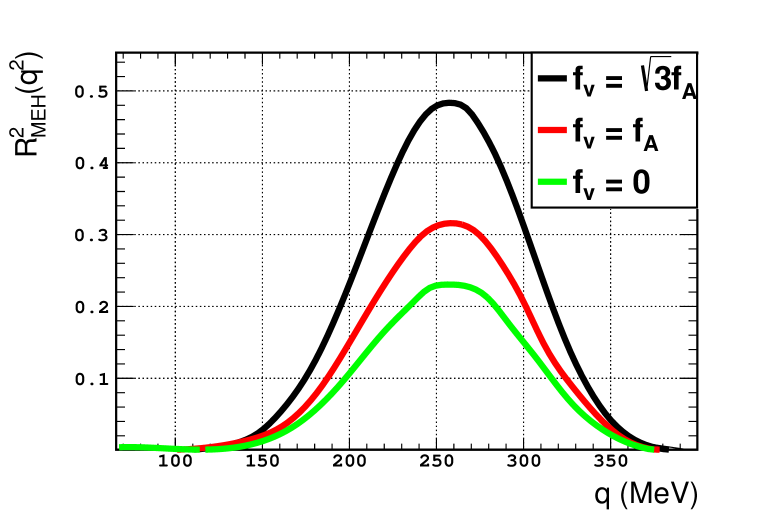
Figure 11: The momentum dependence of $R^{2}_{MEH}(q^{2})$ as a function of $q$ for different values of $f_{V}$. Helm form factors have been used.

VI.3 Some results for ¹⁸⁰Ta

The numerical value of

$$\Lambda\frac{m_{A}}{m_{N}^{2}}\frac{1}{\upsilon^{2}_{0}}\frac{1}{2\pi}$$

in Eq.(45) using Eq.(17) with $f_{A}/f_{V}=1$, is 0.068 for A=180, expressed in units of keV^-1. The plot for $\frac{1}{\upsilon_{0}}\frac{1}{\sigma_{N}}\big{\langle}\upsilon\frac{d\sigma>}{dE_{R}}\big{\rangle}$ versus the previous one multiplied with 0.063. The preference is to express it as a function of $E_{R}$ in units of keV, i.e Fig. 12. It can be shown that a similar expression holds for the rate

$$\frac{1}{R_{N}}\frac{dR}{dE_{R}},$$

see Fig. 13. The expressions for $\sigma_{N}$ and $R$ can be obtained using the relevant values for the nucleon:

$$\sigma_{N}=8.8\cdot 10^{-40}(f_{V}^{2}+3f_{A}^{2}),{\rm\qquad cm^{2}}$$

$$R_{N}=\Phi\sigma_{N}N_{N}=0.72\cdot(f_{V}^{2}+3f_{A}^{2}),\qquad{\rm y^{-1}}$$

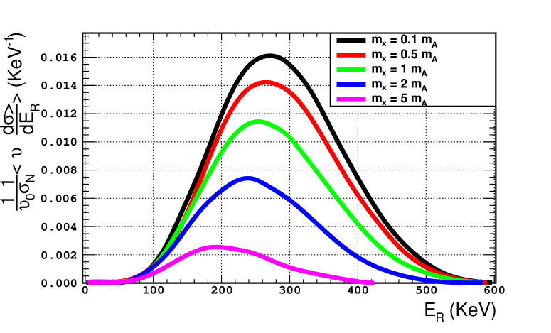
Figure 12: The function $\frac{1}{\upsilon_{0}}\frac{1}{\sigma_{N}}\langle\upsilon\frac{d\sigma>}{dE_{R}}\rangle$ in units of keV^-1. The Helm type form factor has been employed.

One can integrate the differential cross section over the recoil energy $E_{R}$ and multiply with the total nucleon to obtain the WIMP-Nucleus cross section as a function of the WIMP mass $m_{\chi}$ this is exhibited in Fig.  14

The same result holds for the obtained differential rate

$$\frac{1}{R_{N}(m_{\chi})}\frac{dR}{dE_{R}}$$

since the WIMP density used in obtaining the densities is the same. The situation is, however, changed if one is comparing the obtained differential rate relative to the total rate for the nucleon at some fixed value of the WIMP mass. Indeed the obtained differential rate in units total rate of the nucleon for $m_{N}/m_{\chi}=1$ is exhibited in Fig. 13. The exhibited differential rate contains, of course, the WIMP mass dependence arising from the WIMP density in our galaxy.

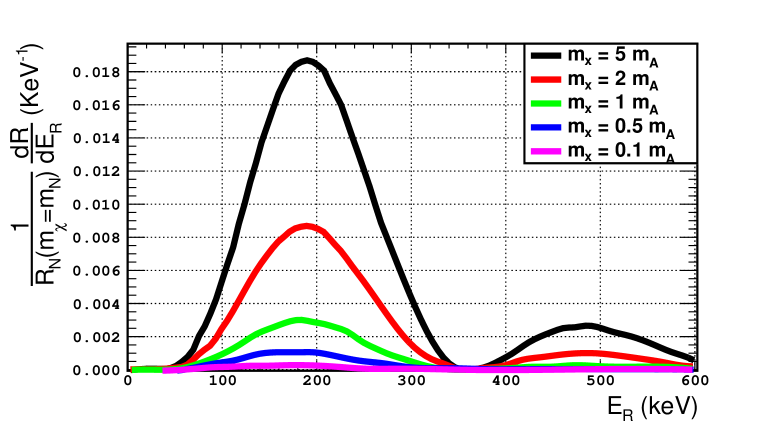
Figure 13: The differential rate relative to the total nucleon rate (for $m_{\chi}=m_{N}$), $\frac{1}{R_{N}(m_{\chi}=m_{N})}\frac{dR}{dE_{R}}$, in units of keV^-1 for the Ta target. The black curve in the drawing has been reduced by a factor of 5, so the related rate must be multiplied by 5. The Helm type form factor has been employed. It also contains the WIMP mass dependence arising from the WIMP density in our galaxy.

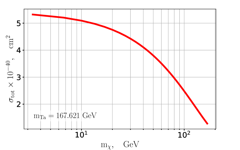
Figure 14: The total WIMP-Nucleus cross section as a function of WIMP mass for the target nucleus $\rm{}^{180m}Ta$.

One can integrate the differential rate over the recoil energy $E_{R}$ and multiply with the total number of nucleons to obtain the the total WIMP-Nucleus event rate as a function of the WIMP mass $m_{\chi}$.

VII Experimental approach for the dark matter search

Calculations performed in previous chapters have been dedicated to the most prominent candidates from the list shown in Tab. 1.

Table 1: Long-lived isomeric states with high spin differences that can be effectively produced and used for the dark matter search.

Isomer	Half-life (year)	Energy (keV)	Spin sequence from I.S. to G.S.	Decay B.R.
102mRh	3.74	140.73 (9)	$6^{+}$ $\rightarrow$ $2^{-}$	$\beta$ $\approx$ 100%
108mAg	438	109.406 (7) (9)	$6^{+}$ $\rightarrow$ $1^{+}$	Isomer tran. 9%
110mAg	0.68	117.59 (5)	$6^{+}$ $\rightarrow$ $2^{-}$ $\rightarrow$ $1^{+}$	Isomer tran. 1.3%
166mHo	1130	5.965 (12)	$7^{-}$ $\rightarrow$ $0^{-}$	$\beta$ $\approx$ 100%
178mHf	31	2446.09 (8)	$16^{+}$ $\rightarrow$ $8^{-}$ $\rightarrow$ $0^{+}$	Isomer tran. $\approx$ 100%
180mTa	$>7\cdot 10^{15}$	76.79 (55)	$9^{-}$ $\rightarrow$ $1^{+}$
186mRe	$2\cdot 10^{5}$	148.2 (5)	$8^{+}$ $\rightarrow$ $1^{-}$	Isomer tran. $>$ 90%
192mIr	241	168.14 (12)	$11^{-}$ $\rightarrow$ $4^{+}$	Isomer tran. $\approx$ 100%
210mBi	$3\cdot 10^{6}$	271.31 (11)	$9^{-}$ $\rightarrow$ $1^{-}$	$\alpha$ $\approx$ 100%
242mAm	141	48.60 (5)	$5^{-}$ $\rightarrow$ $1^{-}$	Isomer tran. $\approx$ 100%

The dark matter collision with the isomeric state has an exceedingly small cross section. Therefore, the isomeric states with longer half-lives are favored due to the smaller contribution of natural decay to their total decay rates. The $\rm{}^{180m}Ta$ is an outstanding candidate for investigation. As mentioned above this nuclide has been proposed [43] and treated by gamma-ray spectrometry with HPGe-detectors [63]. The expected gamma-lines of the direct isomer decay and the further $\rm{}^{180}Ta$ ground state decay (half-life $8.1\leavevmode\nobreak\ \rm h$) are shown in Tab. 2.

Table 2: Transition energies that can arise from the decay of the $9^{-}$ isomeric state of $\rm{}^{180m}Ta$.

Energy (keV)	Transition	Tran. type	Tot. electron CC (Ba)	Electron energy shell (keV)
37.25	180Ta $9^{-}$ $\rightarrow$ 180Ta $2^{+}$	E7	$>$ 108	L26
39.54	180Ta $2^{+}$ $\rightarrow$ 180Ta $1^{+}$	E1	$>$ 0.88	L28.5
76.79	180Ta $9^{-}$ $\rightarrow$ 180Ta $1^{+}$	M8	$>$ 108	K9.37; L65.8
93.30	180Hf $2^{+}$ $\rightarrow$ 180Hf $0^{+}$	E2	4.69	K27.9; L82.8
103.5	180W $2^{+}$ $\rightarrow$ 180W $0^{+}$	E2	1.48	K34
215.3	180Hf $4^{+}$ $\rightarrow$ 180Hf $2^{+}$	E2	0.24	K150
234.0	180W $4^{+}$ $\rightarrow$ 180W $2^{+}$	E2	0.20	K164.5
332.3	180Hf $6^{+}$ $\rightarrow$ 180Hf $4^{+}$	E2	0.060	K267
350.9	180W $6^{+}$ $\rightarrow$ 180W $4^{+}$	E2	0.054	K281,4

The decay energies are precisely determined thanks to the recent accurate measurements of excitation energy of the isomeric state by the Penning trap mass spectrometry: $76.80(33)\leavevmode\nobreak\ \rm keV$ [64]. The energy of transitions expected as a result of the decay of the isomer to the ground state and the daughter nuclides of ${}^{180}\rm W$ and ${}^{180}\rm Hf$ are shown in Tab. 2. Additionally, the values of the internal electron conversion coefficients indicated in the fifth column of Tab. 2. Only the gamma-transition with energy $103.5\leavevmode\nobreak\ \rm keV$ has been used to search for possible response to dark matter [63]. The $93.3\leavevmode\nobreak\ \rm keV$ line from the electron capture is too similar to the background lines from ²³⁴Th. The $\rm 103.5\leavevmode\nobreak\ keV$ gamma-line with the branching ratio $15\%$ registered with the detector efficiency $<0.3\%$ belongs to de-excitation of daughter nuclide ${}^{180}\rm W$. This results in a non-observation of any signal from the DM interaction obtained with HPGe-detector with total photon registration efficiency of $<4\cdot 10^{-4}$.

Meanwhile, Low Temperature Detectors (LTD) are widely used to search for rare events in nuclear and particle physics. Great success was achieved with Magnetic Micro Calorimeters (MMC) [65, 66] that can measure particle and photon energy with detection angle coverage close to $4\pi$. The use of such detectors will increase the sensitivity of recording rare events by many orders of magnitude in comparison with the conventional germanium detector used in [63]. In addition to the angular advantages in such detectors, it is possible to efficiently register the transition energies transmitted by internal conversion electrons, which considerably prevail in the decays of isomeric states with low transition energies. Another very important advantage is the energy resolution, which exceeds the extreme limits of any semiconductor detectors. The MMC-cryogenic detector consists of a metallic absorber that stores the released energy and has a very good connection to the temperature sensor – a paramagnetic alloy, which resides in a low magnetic field. The sensor is weakly connected to a thermal bath. The energy released in the absorber from a radioactive source completely enclosed in the absorber raises the temperature of the detector. This leads to a change of the sensor magnetization which is read out as a change of flux by SQUID magnetometer. Such type of an MMC has been used in the spectra measurement of ${}^{163}\rm Ho$ within the ECHo project [65]. The energy resolution on the level of $1.2\leavevmode\nobreak\ \rm eV$ was achieved at X-ray energy of $6\leavevmode\nobreak\ \rm keV$. The same detector can be used to search for DM-particles with interaction to isomeric state of $\rm{}^{166m}Ho$ (see Tab. 1). This isotope can plentifully be produced in reactors by neutron irradiation of ${}^{165}\rm Ho$. However, the small cross section for the DM-scattering obtained in our calculations for $\rm{}^{166m}Ho$ makes this detection unrealistic due to the strong background contribution of events from natural $\rm{}^{166m}Ho$ radioactive decay.

We emphasize again that $\rm{}^{180m}Ta$ is a promising candidate because its extremely long lifetime has very small background from its natural radioactive decay. Unlike the germanium detector, the MMC-technique allows measurement of all decay channels: characteristic X-ray and gamma-radiation and equally importantly, peaks from internal conversion electrons, which prevail in the spectrum of low-energy transitions, as can be seen in the fourth column of Tab. 2. The last column of the same table shows intensive expected electron energies of these transitions. The most intensive electron spectrum belongs to the energy region below $100\leavevmode\nobreak\ \rm keV$. The most prominent characteristic K X-rays for Ta and Hf nuclides that follow the electron conversion process in the interval from $64.4$ to $67.0\leavevmode\nobreak\ \rm keV$ are beyond the electron conversion spectra and can be also detected by the MMC-detector with high precision of approximately $100\leavevmode\nobreak\ \rm eV$. Thus, in comparison with the germanium detector used in the paper [63], the MMC-method can provide plenty of indicators of DM interactions with the Ta-isomeric state. As a matter of fact some careful elaboration concerning the long-term stability in vacuum and maintenance at low temperature, as well as the physicochemical properties of Ta can be taken into account.

The $\rm{}^{180m}Ta$ isomeric state is the only one in nature, having the abundance of $0.012\%$ in natural tantalum. Isotopic extraction of tantalum is very difficult. However $3\leavevmode\nobreak\ \rm mg$ of isomer diluted in $30\leavevmode\nobreak\ \rm mg$ of $\rm{}^{181}Ta$ was already used in [67]. Hopefully, a similar target is achieved by our proposed experiment instead of the method of [63] in which $180\leavevmode\nobreak\ \rm mg$ of $\rm{}^{180m}Ta$ in $1.5\leavevmode\nobreak\ \rm kg$ of natural tantalum is used. The total achievable mass of $3\leavevmode\nobreak\ \rm mg$ for $\rm{}^{180m}Ta$ corresponds to $N_{N}\approx 10^{19}$ and this value is later used for the half-life calculation in VIII.

Another possibility to produce $\rm{}^{180m}Ta$ is the reaction $(p,pn)$ on $\rm{}^{181}Ta$. Readout system can use SQUID microwave multiplexing [65]. The natural background will be approximately 1 event per year if the expected total lifetime of this isomer is $10^{19}$ year [68]. As can be seen from these estimates, the observation of the DM-effect is very challenging. It becomes more realistic if the cross section attributable to DM de-excitation and/or the natural lifetime of the isomeric state deviate for two-three orders of magnitude from used one. Such deviations are entirely possible. As long as no signature is observed in the long term experiment, limits can be constrain the DM de-excitation. However, if the $\rm{}^{180m}Ta$ decay is observed, then measurements with increased exposure time in deeper underground locations may be indicative of a DM response.

VIII Half-life time estimation

The $\rm{}^{180}Ta$ isomer is predicted to decay to the ground state, but the half-life has not yet been determined. There are only experimental and theoretical upper limits available for this isotope, since decay has never been observed in a real experiment. The expected half-life time should exceed $10^{19}$ years [68]. And the lower experimental bound for the total half-life time is $4.5\cdot 10^{16}$ years (90% C.L.) [69]. The interaction with the WIMP and subsequent decay can be interpreted as normal decay, and from this the half-life time can be estimated.

As shown in the previous section, the overall background is one event per year. Since all dark matter searches do not observe any events (signal is zero), statistical evaluation can be simplified using the conventional Feldman-Cousins approach [70]. The expected number of signal events $n_{exp}$ can be written as

$$n_{exp}=\Phi\cdot\sigma_{\rm tot}\cdot T\cdot N_{N}\cdot\varepsilon,$$ (26)

where $\Phi$ WIMP flux, $\sigma_{\rm tot}$ total cross-section of WIMP isomer interaction, $T$ exposure time, $N_{N}$ number of isomer atoms, $\varepsilon$ detection efficiency. With zero signal this $n_{exp}$ can be associated with a particular upper limit $n_{up}$. For instance in our case the 95% C.L. $n_{up}$ equals 2.33 (signal zero, background one for 1 year exposure [70]).

From another side, signal can be interpreted as normal radioactive decay that follows the exponential decay law. In this case $n_{exp}$ can be expressed as

$$n_{exp}=\varepsilon N_{N}\Big{(}1-\exp{\Big{[}-\ln{2}\cdot\frac{T}{T_{1/2}}\Big{]}}\Big{)}\simeq\frac{\varepsilon N_{N}T}{T_{1/2}}\cdot\ln{2},$$ (27)

with expected half-life time $T_{1/2}$. Combining Eq. (26) and Eq. (27), we can express $T_{1/2}$ as a function of $T$

$$T_{1/2}=\frac{T\cdot\ln{0.5}}{\ln{(1-\Phi\sigma T)}}\simeq\frac{\ln{2}}{\Phi\sigma}$$ (28)

As can be seen, the $T_{1/2}$ does not depend on the amount of isomer and detection efficiency, because in our case the cross-section is already determined from theory. Based on that, we can estimate the sensitivity of the proposed experimental setup to the WIMP-nucleon interaction, where the last one can be interpreted as normal radioactive decay.

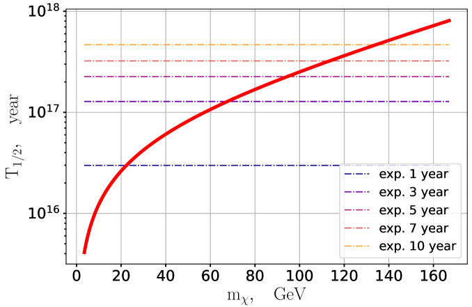
Figure 15: The solid red line is the half-life time as a function of the WIMP mass for $\rm{}^{180m}Ta$. Dashed lines indicate 95% C.L. sensitivity for the proposed experimental setup with different exposures. Assumed parameters for calculating sensitivity $\varepsilon=0.01$, $N_{N}=10^{19}$.

In Fig. 15 the half-life time of $\rm{}^{180m}Ta$ as function of WIMP mass is depicted. Several levels of the experimental sensitivity with different exposure time are also shown. We can conclude that the WIMP-nucleon interaction can be measured with 95% C.L. for masses $\leq 130$ GeV (10 years exposure time is assumed). The conservative value of the detector efficiency was chosen as 1%, and the result depends linearly from $\varepsilon$, hence it can be easily scaled for higher values of $\varepsilon$.

IX Discussion

We have seen that, not unexpectedly, the nuclear ME encountered in the inelastic WIMP-nucleus scattering involving isomeric nuclei is much smaller than that involved in the elastic process considered in the standard WIMP searches. This occurs for two reasons: a) the form factor in the elastic being favorable, see Fig. 2, and b) in the elastic case the cross section is proportional to the mass number $A^{2}$. In the present case the nuclear matrix element for $\rm{}^{180}Ta$, as indicated by the coefficients appearing in Eq. (24), is not unusually small compared to other typical inelastic processes. The Nilsson model is expected to work well in the case of $\rm{}^{180}Ta$, but the obtained event rate is quite small.

Following the estimated WIMP-nucleon cross section and the current mass of $\rm{}^{180}Ta$ isomer ($N_{N}\approx 10^{19}$), the estimated half-life time is between $10^{15}$ and $10^{18}$ years, covering current experimental limit $4.5\cdot 10^{16}$ years (90% C.L.) [69]. However it is still not enough to reach the expected half-life time for $\rm{}^{180m}Ta$. That is why various experimental approaches are required to disentangle this puzzle. Further improvement can be achieved using larger mass of isomer with better detection efficiency. At the same time, the experiment can exploit the signal provided by the subsequent standard decay of the $2^{+}$ state to the ground state, that is not available in the conventional WIMP searches.

Appendix A Recoil energy calculation

Let us estimate the maximum recoil energy. From Eq. (6) we find the maximum momentum is given by:

$$\frac{1}{q_{\rm max}}\Big{(}\frac{q_{\rm max}^{2}}{2\mu_{r}}-\Delta\Big{)}=\upsilon_{\rm esc}$$ (29)

The only acceptable solution is

$$q_{\rm max}=\mu_{r}\upsilon_{\rm esc}\left[1+\sqrt{1+\frac{2\Delta}{\mu_{r}\upsilon^{2}_{\rm esc}}}\right]$$ (30)

Thus the maximum recoil energy is given by

$$\left(E_{R}\right)_{\rm max}=\frac{1}{2m_{A}}q_{\rm max}^{2}=\frac{1}{2}m_{A}\upsilon_{\rm esc}^{2}\frac{1}{(1+x)^{2}}\left[1+\sqrt{1+\frac{\Delta(1+x)}{\frac{1}{2}m_{A}\upsilon_{\rm esc}^{2}}}\right]^{2},\quad x=\frac{m_{A}}{m_{\chi}}$$ (31)

In the special case of elastic scattering ($\Delta=0$), we find the expected results

$$\left(E_{R}\right)_{\rm max}=2m_{A}\upsilon_{\rm esc}^{2},\leavevmode\nobreak\ m_{\chi}>>m_{A},\leavevmode\nobreak\ \left(E_{R}\right)_{\rm max}\approx 0,\leavevmode\nobreak\ m_{A}>>m_{\chi},\leavevmode\nobreak\ \left(E_{R}\right)_{\rm max}=\frac{1}{2}m_{A}\upsilon_{\rm esc}^{2},\leavevmode\nobreak\ m_{A}\approx m_{\chi}$$ (32)

In the case of $\Delta>0$ we find that for $m_{\chi}\approx m_{A}$

$$\left(E_{R}\right)_{\rm max}=\frac{1}{8}m_{A}\upsilon_{\rm esc}^{2}\left[1+\sqrt{1+\frac{2\Delta}{\frac{1}{2}m_{A}\upsilon_{\rm esc}^{2}}}\right]^{2}\approx 0.5\cdot 10^{-6}m_{A}\left[1+\sqrt{1+\frac{\Delta}{2\cdot 10^{-6}m_{A}}}\right]^{2},\,m_{A}\approx m_{\chi}$$ (33)

Appendix B The differential cross section for the inelastic WIMP-nucleus scattering

Eq.(11), using Eq.(13), can be cast in the form:

$$d\sigma=\Lambda\frac{\sigma_{N}}{m_{N}^{2}}\frac{1}{\upsilon}\frac{1}{(2\pi)^{2}}d^{3}{\bf q}\delta\left(\frac{q^{2}}{2\mu_{r}}-q\upsilon\xi-\Delta\right)\frac{|ME(q^{2})|^{2}|}{f_{V}^{2}+3f_{A}^{2}}$$ (34)

Where

$$\Lambda=\frac{2\pi}{4}.$$

Folding Eq.(34) with the velocity distribution we find

$$\begin{split}\frac{1}{\upsilon_{0}}\frac{1}{\sigma_{N}}\langle\upsilon\frac{d\sigma}{dE_{R}}\rangle=&\Lambda\frac{m_{A}}{m_{N}^{2}}\frac{1}{\upsilon_{0}}\frac{1}{2\pi}\frac{|ME(q^{2})|^{2}}{f_{V}^{2}+3f_{A}^{2}}\\ &\left[\left(\Theta\left(\Delta-\frac{M_{A}E_{R}}{\mu_{r}}\right)\right)\int_{\upsilon_{1}}^{\upsilon_{\rm esc}}K(\upsilon)d\upsilon+\left(\Theta\left(-\Delta+\frac{M_{A}E_{R}}{\mu_{r}}\right)\right)\int_{\upsilon_{2}}^{\upsilon_{\rm esc}}K(\upsilon)d\upsilon\right]\end{split}$$ (35)

where $E_{R}$ is the nuclear recoil energy and $K(\upsilon)$ given by the velocity distribution

$$K(\upsilon)=\int d\Omega(\hat{\upsilon})\upsilon f_{\rm distr}(\bm{v})$$ (36)

and $\Theta$ is the step function:

$$\Theta(x)=\left\{\begin{array}[]{cc}1,&x>0\\ 0,&x<0\\ \end{array}\right.$$ (37)

Furthermore

$$\upsilon_{1,2}=\pm\leavevmode\nobreak\ \frac{1}{q}\Big{(}\Delta-\frac{q^{2}}{2\mu_{r}}\Big{)}$$ (38)

Note the dependence of the cross section on the recoil energy comes in two ways: i) From the nuclear form factor and ii) from the minimum required velocities $\upsilon_{1}$ and $\upsilon_{2}$ in the folding with the velocity distribution.

We will specialize our results in the commonly used Maxwell- Boltzmann (MB) distribution in the local frame

$$f_{MB}=\frac{1}{\pi^{3/2}}\frac{1}{\upsilon^{3}_{0}}e^{-(y^{2}+2y\xi+1)},\quad y=\frac{\upsilon}{\upsilon_{0}}$$ (39)

where $\upsilon_{0}$ is the velocity of the sun around the center of the galaxy and $\xi$ the angle between $\bm{v}$ and the direction of sun’s motion. Then

$$K(\upsilon)=\frac{2}{\sqrt{\pi}}e^{-(y^{2}+1)}y\int_{-1}^{1}e^{-2y\xi}=\frac{2}{\sqrt{\pi}}e^{-(y^{2}+1)}\sinh{2y}$$ (40)

$$\begin{split}&\frac{1}{\upsilon_{0}}\frac{1}{\sigma_{N}}\langle\upsilon\frac{d\sigma>}{dE_{R}}\rangle=\Lambda\frac{m_{A}}{m_{N}^{2}}\frac{1}{\upsilon^{2}_{0}}\frac{1}{2\pi}\frac{|ME(q^{2})|^{2}|}{f_{V}^{2}+3f_{A}^{2}}\\ &\left[\left(\Theta\left(\Delta-\frac{M_{A}E_{R}}{\mu_{r}}\right)\right)\int_{y_{1}}^{y_{\rm esc}}e^{-(y^{2}+1)}\sinh{2y}dy+\left(\Theta\left(-\Delta+\frac{M_{A}E_{R}}{\mu_{r}}\right)\right)\int_{y_{2}}^{y_{\rm esc}}e^{-(y^{2}+1)}\sinh{2y}dy\right]\end{split}$$ (41)

The above integrals can by computed analytically

$$\begin{split}\frac{1}{\upsilon_{0}}\frac{1}{\sigma_{N}}\langle\upsilon\frac{d\sigma}{dE_{R}}\rangle=&\Lambda\frac{m_{A}}{m_{N}^{2}}\frac{1}{\upsilon^{2}_{0}}\frac{1}{2\pi}\frac{|ME(q^{2})|^{2}|}{f_{V}^{2}+3f_{A}^{2}}\\ &\left[\left(\Theta\left(\Delta-\frac{M_{A}E_{R}}{\mu_{r}}\right)\right)\psi_{1}(y_{1},y_{\rm esc})+\left(\Theta\left(-\Delta+\frac{M_{A}E_{R}}{\mu_{r}}\right)\right)\psi_{2}(y_{2},y_{\rm esc})\right]\end{split}$$ (42)

where

$$\begin{split}\psi_{i}(y_{i},y_{\rm esc})&=\frac{1}{4}\sqrt{\pi}\left(\text{erf}\left(1-y_{i}\right)+\text{erf}\left(y_{i}+1\right)\right)-\frac{1}{4}\sqrt{\pi}\left(\text{erf}\left(1-y_{\rm esc}\right)+\text{erf}\left(y_{\rm esc}+1\right)\right),\quad i=1,2\end{split}$$ (43)

The functions $\psi_{i}(y_{i},y_{\rm esc})$ depend on the momentum transfer. This depends on the specific nuclear target and will be discussed below. The expression contained in the last square bracket is momentum dependent and provides a restriction in the range and distribution of momentum. It is given by Figs. 7 and 16 for the nuclei of interest in this work.

Sometimes is useful to modify the above formulas using dimensionless variables. let us define $\eta=qR$, where is the nuclear radius. Then

$$\frac{1}{q}\Big{(}\frac{q^{2}}{2\mu_{r}}-\Delta\Big{)}=\left(\frac{1}{2}(1+x)\frac{\eta^{2}}{m_{A}R^{2}}-\Delta\right)\frac{R}{\eta}=\frac{1}{2}(1+x)\frac{\eta}{a}-\frac{b}{\eta},\leavevmode\nobreak\ a=m_{A}R,\leavevmode\nobreak\ b=\Delta R$$

Thus

$$y_{1}=\frac{c}{\upsilon_{0}}\left(-\frac{1}{2}(1+x)\frac{\eta}{a}+\frac{b}{\eta}\right),\,y_{2}=\frac{c}{\upsilon_{0}}\left(\frac{1}{2}(1+x)\frac{\eta}{a}-\frac{b}{\eta}\right)$$ (44)

$$\begin{split}\frac{1}{\upsilon_{0}}\frac{1}{\sigma_{N}}\langle\upsilon\frac{d\sigma>}{dE_{R}}\rangle=&\Lambda\frac{m_{A}}{m_{N}^{2}}\frac{1}{\upsilon^{2}_{0}}\frac{1}{2\pi}\frac{|ME(q^{2})|^{2}|}{f_{V}^{2}+3f_{A}^{2}}\\ &\left[\left(\Theta\left(b-\frac{1}{2}(1+x)\frac{\eta^{2}}{a}\right)\right)\psi_{1}(y_{1},y_{\rm esc})+\left(\Theta\left(-b+\frac{1}{2}(1+x)\frac{\eta^{2}}{b}\right)\right)\psi_{2}(y_{2},y_{\rm esc})\right]\end{split}$$ (45)

where the functions $\psi_{1}$ and $\psi_{2}$ are given by Eq.(43) via Eq.(44).

In shell model calculations instead of the nuclear radius $R$ one may use the harmonic oscillator size parameter $b_{A}$ (see Appendix E). There remains the crucial part of the calculation in involving the nuclear matrix element and the associated nuclear form factor.

Appendix C The nucleon cross section and event rate

We have seen that Eq.(12) is correct, but it does not indicate the range of $q$ involved. To find it we return to the basic expression $\frac{q^{2}}{2mu_{2}}-q\upsilon\xi=0$. This leads to

$$\xi=\frac{q}{2\mu_{2}}{\upsilon}<1\Rightarrow\upsilon>\upsilon_{min},\quad\upsilon_{min}=\frac{\sqrt{2m_{N}E_{R}}}{2m_{N}}(1+x)=\sqrt{\frac{E_{R}}{2m_{N}}}(1+x)$$ (46)

This implies that

$$y_{min}=\sqrt{\frac{E_{R}}{2m_{N}\upsilon_{0}^{2}}}(1+x)$$ (47)

Folding expression of Eq.(12) with the velocity distribution, we obtain

$$\langle\upsilon d\sigma_{N}(\upsilon)\rangle=\int_{\upsilon_{min}}^{\upsilon_{\rm esc}}\upsilon d\sigma_{N}(\upsilon)f_{dist}(\bm{v})d^{3}\bm{v}$$ (48)

For a Maxwell-Boltzmann distribution, see Eq.(39), one can show that :

$$\langle d\sigma_{N}(\upsilon)\rangle=Sp\,dE_{R}\,\upsilon_{0}\frac{2}{\sqrt{\pi}}\int_{y_{min}}^{y_{\rm esc}}yf_{MB}dy,\,Sp=\frac{1}{\upsilon^{2}_{0}}\frac{1}{2\pi}m_{N}\left(\frac{G_{F}}{\sqrt{2}}\right)^{2}|ME_{N}|^{2}$$ (49)

where the factors $\upsilon_{0}$ have been separated judiciously (in dark matter searches the factor $\upsilon_{0}$ is absorbed in the WIMP flux (rate=flux $\times$ cross section).
Performing the integration over $y$ we find

$$\langle d\sigma_{N}(\upsilon)\rangle=\upsilon_{0}\psi(y_{min},y_{\rm esc})Sp.$$ (50)

with

$$\psi(y_{min},y_{\rm esc})=\frac{1}{4}\sqrt{\pi}\left(-\text{erf}\left(1-y_{\text{\rm esc}}\right)-\text{erf}\left(y_{\text{\rm esc}}+1\right)+\text{erf}\left(1-y_{min}\right)+\text{erf}\left(y_{\min}+1\right)\right)$$ (51)

$$y_{min}=\sqrt{\frac{E_{R}}{2m_{N}\upsilon_{0}^{2}}}(1+x)=\sqrt{\frac{E_{R}}{\mbox{keV}}}(1+x)$$

We must now integrate over the recoil energy from zero to $(E_{R})_{\rm max}$ given by Eq.(9)

$$\langle\sigma_{N}(\upsilon)\rangle=\upsilon_{0}(4m_{N}\upsilon^{2}_{0})\,Sp\phi(x),\,\phi(x)=\int_{0}^{(E_{R})_{\rm max}}dE_{R}\psi(y_{min},y_{\rm esc}).$$ (52)

The function can only be obtained numerically. It is exhibited in Fig. 19. It is clear that for values of $m_{\chi}$ much larger than $m_{N}$ the cross section becomes independent of $m_{\chi}$ .

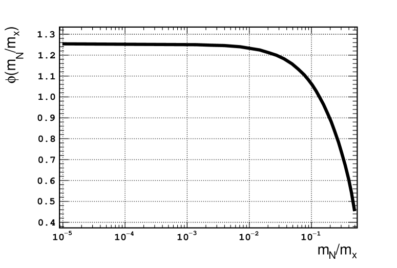
Figure 19: The dependence on the function $\phi(x)$ on the mass $m_{\chi}$ appearing in the case of the nucleon-WIMP scattering

Adopting the value $\phi(x)\approx 1$ we obtain:

$$\langle\sigma_{N}(\upsilon)\rangle=\upsilon_{0}\,4.0\,\frac{1}{2\pi}m^{2}_{N}\left(\frac{G_{F}}{\sqrt{2}}\right)^{2}|ME_{N}|^{2}$$ (53)

The WIMP-nucleon interaction is not known. Let us assume that it is of $V-A$ type in dimensionless units. Then

$$|ME_{N}|^{2}=|ME_{F}|^{2}+|ME_{A}|^{2}=f_{V}^{2}+f_{A}^{2}\langle N|\bm{s}|N\rangle^{2}=f_{V}^{2}+3f_{A}^{2}$$ (54)

Thus, if we absorb the factor $\upsilon_{0}$ into the flux, we can write the effective total cross section becomes:

$$\sigma_{N}=4.0\frac{1}{2\pi}m^{2}_{N}\left(\frac{G_{F}}{\sqrt{2}}\right)^{2}\left(f_{V}^{2}+3f_{A}^{2}\right)$$ (55)

$\sigma_{N}=3,3\times 10^{-39}(f_{V}^{2}+3f_{A}^{2})$
For calculating the rates in addition to the cross section one needs the flux of the oncoming particles and the number of particles in the target. For an estimate we will consider $N_{N}=10^{24}$ particles in the target. The WIMP energy density in our vicinity is $\rho=0.3$ $\rm GeV\cdot cm^{-3}$, leading to a particle density $N_{\chi}=\frac{\rho}{m_{\chi}}=\frac{\rho}{m_{N}}x$ with $x=\frac{m_{N}}{m_{\chi}}$
The flux is the particle density times the WIMP velocity:

$$\Phi=N_{\chi}\upsilon=\frac{\rho}{m_{\chi}}\upsilon_{0}=\frac{\rho}{m_{N}}\upsilon_{0}x=(0.3\times(220\times 10^{3}\times 10^{2})\times 3.157\times 10^{7}y^{-1}x=2.1\times 10^{14}\mbox{cm}^{-2}y^{-1}x$$ (56)

The combined effect on the rate is

$$f_{R}=\Phi N_{N}\sigma_{N}=2.1\times 10^{38}\mbox{cm}^{-2}y^{-1}x\times 3.3\times 10^{-39}(f_{V}^{2}+3f_{A}^{2})$$ (57)

Thus

$$f_{R}=0.72y^{-1}x(f_{V}^{2}+3f_{A}^{2})$$

for $m_{\chi}=m_{N}$ as reference we obtain the rate:

$$R=0.72\mbox{y}^{-1}(f_{V}^{2}+3f_{A}^{2})$$ (58)

A similar procedure can applied in the WIMP-nucleus-scattering with the obvious modification $m_{N}\rightarrow m_{A}$.

Appendix D The Reduced nuclear ME for a two particle system

As we have seen, the two particle proton- neutron system of the type considered here can be described in terms of one proton and one neutron Nilsson orbitals. These can be expanded in a spherical basis. The reduced nuclear matrix element (RNME) of WIMP-nuclear transition can be obtained using the well known Racah techniques.
i) The RNME in the case of $\rm{}^{180}Ta$ target.
Since the initial state is of negative parity involving a proton in a negative parity state, while the final state considered here is of positive parity, the interaction involves only the proton component with neutron being a spectator particle. Thus the reduced nuclear matrix takes the form:

$$\langle[j^{\prime}_{1}j_{2}]J_{f}||T^{[\lambda\otimes s]J}||[j_{1}j_{2}]J_{i}\rangle=\sqrt{\frac{2J_{f}+1}{2j^{\prime}_{1}+1}}U[j_{1},j_{2},J_{i},J,0,J,j^{\prime}_{1}j_{2},J_{]}]\langle j^{\prime}_{1}||T^{[\lambda\otimes s]}||j_{1}\rangle$$ (59)

where $U[\cdots]$ is the unitary Nine-J symbol, see e.g. [61]. Furthermore:

$$\langle j^{\prime}_{1}||T^{[\lambda\otimes s]J}||j_{1}\rangle=\sqrt{2j^{\prime}_{1}+1}U[\ell_{1},1/2,j_{1},\lambda,s,J,\ell^{\prime}_{1},1/2,j^{\prime}_{1}]\frac{\langle\ell^{\prime}_{1}||\sqrt{4\pi+1}Y^{\lambda}||\ell_{1}\rangle}{\sqrt{2\ell^{\prime}_{1}+1}}\times\begin{array}[]{cc}f_{V},s=0\\ f_{A}\sqrt{3},s=1\\ \end{array}$$ (60)

The last reduced ME is essentially that of the spherical harmonic

$$\langle\ell^{\prime}_{1}||\sqrt{4\pi+1}Y^{\lambda}||\ell_{1}\rangle=\sqrt{(2\ell_{1}+1)(2\lambda+1)}\langle\ell_{1},0;\lambda,0|\ell^{\prime}_{1},0\rangle\langle n^{\prime}_{1}\ell^{\prime}_{1}|j_{\lambda}(kr)|n_{1}\ell_{1}\rangle\Rightarrow$$ (61)

$$\begin{split}&\langle[j^{\prime}_{1}j^{\prime}_{2}]J_{f}||T^{[\lambda\otimes s]J}||[j_{1}j_{2}]J_{i}\rangle=\\ &\delta_{j_{2},j^{\prime}_{2}}\sqrt{2J_{f}+1}U[j_{1},j_{2},J_{i},J,0,J,j^{\prime}_{1}j_{2},J_{f}]U[\ell_{1},1/2,j_{1},\lambda,s,J,\ell^{\prime}_{1},1/2,j^{\prime}_{1}]\frac{\sqrt{(2\ell_{1}+1)(2\lambda+1)}}{\sqrt{(2\ell^{\prime}_{1}+1)}}\times\\ &\langle\ell_{1},0;\lambda,0|\ell^{\prime}_{1},0\rangle\langle n^{\prime}_{1}\ell^{\prime}_{1}|j_{\lambda}(kr)|n_{1}\ell_{1}\rangle\end{split}$$ (62)

ii)The case of interacting protons and neutrons.
In case that both protons and neutron can interact the above expression can be written compactly as follows

$$\begin{split}&\langle[j^{\prime}_{1}j^{\prime}_{2}]J_{f}||T^{[\lambda\otimes s]J}||[j_{1}j_{2}]J_{i}\rangle=\\ &\sqrt{2J_{f}+1}\left(\delta_{j_{2},j^{\prime}_{2}}U[j_{1},j_{2},J_{i},J,0,J,j^{\prime}_{1}j^{\prime}_{2},J_{f}]ff(j_{1},j^{\prime}_{1})+\delta_{j_{1},j^{\prime}_{1}}U[j_{1},j_{2},J_{i},0,J,J,j^{\prime}_{1}j^{\prime}_{2},J_{f}]ff(j_{2},j^{\prime}_{2})\right)\end{split}$$ (63)

with

$$ff(j_{i},j^{\prime}_{i})=\frac{\sqrt{(2\ell_{i}+1)(2\lambda+1)}}{\sqrt{(2\ell^{\prime}_{i}+1)}}U[\ell_{i},1/2,j_{i},\lambda,s,J,\ell^{\prime}_{i},1/2,j^{\prime}_{i}]\langle\ell_{i},0;\lambda,0|\ell^{\prime}_{i},0\rangle\langle n^{\prime}_{i}\ell^{\prime}_{i}|j_{\lambda}(kr)|n_{i}\ell_{i}\rangle,\quad i=1,2$$ (64)

A detailed explicit calculation reduced matrix elements in the case of ¹⁶⁶Ho is given in section D.1.

D.1 The explicit calculation reduced matrix elements in the case of $\rm{}^{166}Ho$

Using standard Racah techniques one finds [61]:

$$\begin{split}RME=&C^{2}_{0h_{11/2}}C^{2}_{0g_{11/2}}\left[\begin{array}[]{ccc}1_{1}/2&11/2&0\\ 7&0&7\\ 11/2&11/2&7\\ \end{array}\right]\\ &\frac{\langle 0g11/2||^{T(\lambda,J)}||0g{11/2}\rangle}{\sqrt{12}}+\frac{C_{0g_{13/2}}}{C^{2}_{0g_{11/2}}}\frac{\langle 0g11/2||T^{(\lambda,J)}||0g_{13/2}\rangle}{\sqrt{12}}\sqrt{\frac{7}{6}}-\frac{\langle 0h11/2||T^{(\lambda,J)}||0h_{11/2}\rangle}{\sqrt{12}}\end{split}$$ (65)

the unitary nine-j being $1/\sqrt{15}$.

$$\frac{\langle 0g11/2||^{T(\lambda,J)}||0g{11/2}\rangle}{\sqrt{12}}=\left[\begin{array}[]{ccc}6&1/2&11/2\\ \lambda&1&J\\ 6&1/2&11/2\\ \end{array}\right]\frac{\langle 6||\sqrt{4\pi}Y^{\lambda}||6\rangle}{\sqrt{13}}\frac{\langle 1/2|||\bm{\sigma}||1/2\rangle}{\sqrt{3}}=$$

$$\left[\begin{array}[]{ccc}6&1/2&11/2\\ \lambda&1&J\\ 6&1/2&11/2\\ \end{array}\right]\sqrt{2\lambda+1},\langle(6,0),(\lambda,0)(6.0)\rangle\sqrt{3}=\begin{array}[]{cc}140\sqrt{\frac{5}{46189}},&\lambda=8\\ \frac{10\sqrt{\frac{70}{209}}}{13},&\lambda=6\\ \end{array}$$

with the unitary nine-j being $2\sqrt{\frac{70}{263}}$ and $-\frac{1}{13}\sqrt{\frac{35}{6}}$ for $\lambda$=8 and 6 respectively.
The expression for the $\frac{\langle 0g11/2||^{T(\lambda,J)}||0g{13/2}\rangle}{\sqrt{12}}$ is similar except that now the nine-j are $-\sqrt{\frac{35}{442}}$ and $-\frac{4}{13}\sqrt{\frac{10}{7}}$ for $\lambda=8$ and 6 respectively.
Furthermore

$$\frac{\langle 0h11/2||^{T(\lambda,J)}||0h{11/2}\rangle}{\sqrt{12}}=\left[\begin{array}[]{ccc}5&1/2&11/2\\ \lambda&1&J\\ 5&1/2&11/2\\ \end{array}\right]\frac{\langle 5||\sqrt{4\pi}Y^{\lambda}||5\rangle}{\sqrt{11}}\frac{\langle 1/2|||\bm{\sigma}||1/2\rangle}{\sqrt{3}}=$$

$$\left[\begin{array}[]{ccc}5&1/2&11/2\\ \lambda&1&J\\ 5&1/2&11/2\\ \end{array}\right]\sqrt{2\lambda+1},\langle(5,0),(\lambda,0)(5.0)\rangle\sqrt{3}\begin{array}[]{cc}-28\sqrt{\frac{5}{46189}},&\lambda=8\\ -\frac{2\sqrt{\frac{1330}{11}}}{13},&\lambda=6\\ \end{array}$$

now the relevant nine-j are $-2\sqrt{\frac{2}{561}}$ and $\sqrt{\frac{95}{858}}$ for $\lambda$=8 and 6 respectively.

D.2 The explicit calculation reduced matrix elements in the case of ¹⁸⁰Ta

i) Vector matrix element.

$$VME=\frac{f_{V}}{f_{A}}(1.52946F_{6,5,7}(u)+1.79799F_{6,5,9}(u)+2.19718F_{6,5,11}(u)+1.52946F_{6,3,7}(u)+$$

$$1.52946F_{6,3,9}(u),1.01419+F_{4,5,7}(u)+1.01419F_{4,5,9}(u)-0.06445F_{4,3,7}(u))$$

i) Axial vector matrix element.

$$AME=-2.04512F_{6,5,7}-2.31181F_{6,5,9}(u)-3.58938F_{6,5,11}(u)-2.04512F_{6,3,7}(u)$$

$$-3.3217F_{6,3,9}(u)-2.05117F_{4,5,7}(u)-2.16715F_{4,5,9}(u)-0.3215F_{4,3,7}(u)$$

Appendix E The shell model nuclear form factors

The needed form factors $FF_{\ell\lambda}(u)$ are as follows
i) The case of $\rm{}^{166}Ho$.

$$FF_{6,8}(u)=\frac{e^{-\frac{u^{2}}{4}}u^{8}\left(u^{4}-84u^{2}+1596\right)}{8648640},\,FF_{6,6}(u)=-\frac{e^{-\frac{u^{2}}{4}}u^{6}\left(u^{6}-114u^{4}+3876u^{2}-38760\right)}{8648640},$$

$$FF_{5,8}(u)=-\frac{e^{-\frac{u^{2}}{4}}u^{8}\left(u^{2}-38\right)}{332640},\,FF_{5,6}(u)\frac{e^{-\frac{u^{2}}{4}}u^{6}\left(u^{4}-68u^{2}+1020\right)}{332640}$$

with $u=b_{N}(A)q$ with $b_{N}(A)$, the harmonic oscillator size parameter given, by:

$$b_{N}(A)\approx 1.00\sqrt[6]{A}$$ (66)

The first index specifies the interaction orbit (the transition is diagonal) and the second index corresponds to the multipolarity $\lambda$.

ii) The case of $\rm{}^{180}Ta$.
One can also calculate the odd parity form factors analytically. The resulting expressions are rather complicated to present here. We are satisfied with exhibiting our results in Fig. 8.

iii) In the case of the Helm type form factors one uses the nuclear radius

$$R(A)=1.24\cdot A^{1/3}$$ (67)

Appendix F Some useful expansions of Nilsson levels to shell model states

Table 3: Expansions of neutron Nilsson orbitals $\Omega[Nn_{z}\Lambda]$ in the shell model basis $|Nlj\Omega\rangle$ for three different values of the deformation $\epsilon$.

${7\over 2}[633]$
$|Nlj\Omega\rangle$	$\left|64{7\over 2}{7\over 2}\right\rangle$	$\left|64{9\over 2}{7\over 2}\right\rangle$	$\left|66{11\over 2}{7\over 2}\right\rangle$	$\left|66{13\over 2}{7\over 2}\right\rangle$
$\epsilon$
0.05	$-0.0012$	0.0544	$-0.0166$	0.9984
0.22	$-0.0161$	0.1927	$-0.0744$	0.9783
0.30	$-0.0254$	0.2380	$-0.1000$	0.9658

${9\over 2}[624]$
$|Nlj\Omega\rangle$		$\left|64{9\over 2}{9\over 2}\right\rangle$	$\left|66{11\over 2}{9\over 2}\right\rangle$	$\left|66{13\over 2}{9\over 2}\right\rangle$
$\epsilon$
0.05		0.0336	$-0.0176$	0.9993
0.22		0.1120	$-0.0724$	0.9911
0.30		0.1366	$-0.0947$	0.9861

${5\over 2}[512]$
$|Nlj\Omega\rangle$	$\left|53{5\over 2}{5\over 2}\right\rangle$	$\left|53{7\over 2}{5\over 2}\right\rangle$	$\left|55{9\over 2}{5\over 2}\right\rangle$	$\left|55{11\over 2}{5\over 2}\right\rangle$
$\epsilon$
0.05	0.0659	0.2016	0.9772	0.0047
0.22	$-0.0242$	0.8371	0.5231	$-0.1580$
0.30	$-0.0619$	0.8684	0.4439	$-0.2123$

Table 4: Expansions of proton Nilsson orbitals $\Omega[Nn_{z}\Lambda]$ in the shell model basis $|Nlj\Omega\rangle$ for three different values of the deformation $\epsilon$.

${7\over 2}[523]$
$|Nlj\Omega\rangle$	$\left|53{7\over 2}{7\over 2}\right\rangle$	$\left|55{9\over 2}{7\over 2}\right\rangle$	$\left|55{11\over 2}{7\over 2}\right\rangle$
$\epsilon$
0.05	0.0323	$-0.0212$	0.9993
0.22	0.1129	$-0.0872$	0.9898
0.30	0.1398	$-0.1138$	0.9836

${9\over 2}[514]$
$|Nlj\Omega\rangle$	$\left|55{9\over 2}{9\over 2}\right\rangle$	$\left|55{11\over 2}{9\over 2}\right\rangle$
$\epsilon$
0.05	$-0.0194$	0.9998
0.22	$-0.0716$	0.9974
0.30	$-0.0907$	0.9959