Learning Local Control Barrier Functions
for Safety Control of Hybrid Systems

Abstract

Hybrid dynamical systems are ubiquitous as practical robotic applications often involve both continuous states and discrete switchings. Safety is a primary concern for hybrid robotic systems. Existing safety-critical control approaches for hybrid systems are either computationally inefficient, detrimental to system performance, or limited to small-scale systems. To amend these drawbacks, in this paper, we propose a learning-enabled approach to construct local Control Barrier Functions (CBFs) to guarantee the safety of a wide class of nonlinear hybrid dynamical systems. The end result is a safe neural CBF-based switching controller. Our approach is computationally efficient, minimally invasive to any reference controller, and applicable to large-scale systems. We empirically evaluate our framework and demonstrate its efficacy and flexibility through two robotic examples including a high-dimensional autonomous racing case, against other CBF-based approaches and model predictive control.

I Introduction

Consider the following safety-critical scenarios: 1) automated vehicles switching from eco driving mode to sport driving mode; 2) bipedal robots walking in the warehouse to assist human; and 3) autonomous drones flying from high-pressure area to low-pressure area. The common feature of these ubiquitous autonomous systems is that they are all hybrid dynamical systems, which involve both continuous state evolution and discrete mode switching. Such discrete mode switching can be actively triggered by high-level logical decision-making or passively induced by sudden changes in the underlying physical environments.

Safety-critical control is one of the fundamental problems for hybrid dynamical systems. In the past decades, many approaches have been proposed to guarantee safety for hybrid systems such as model predictive control (MPC) [1] and Hamilton-Jacobi reachability (HJ-reach) [2, 3]. MPC provides safety guarantees by encoding safety constraints in a receding horizon optimization problem, which suffers from high online computation cost though, especially when the dynamics is nonlinear or the horizon is large. HJ-reach methods compute optimal safe controllers by solving PDEs through dynamic programmings, which are difficult to be applied to high-dimensional systems. Other approaches, such as computing controlled invariant sets [4], are also difficult to be applied to general nonlinear systems.

Control barrier function (CBF) [5, 6, 7] recently emerges as a promising approach since it can explicitly specify a safe control set and enforce the invariance of safe sets. This is achieved by constructing a CBF-based safety filter that projects unsafe reference control into the safe control set. Compared with MPC and HJ-reach, CBF enjoys low computation cost and can be applied to any reference controller as a flexible safety filter. In the context of safety control for hybrid systems, [8, 9] propose to use a common CBF that ensures safety for all modes to ensure gloabl safety. However, such common/global CBF may be overall conservative to deteriorate the system performance.

In our recent work [10], we propose a local CBFs-based approach to address the safety control problem for hybrid systems. Specifically, we assume that, for each dynamical mode of the hybrid system, there already exists a CBF that can ensure safety locally within this model. However, it is discovered that local safety for each mode is not sufficient to ensure safety globally as unsafe behaviors may occur under discrete jumps. To address this issue, safe switching sets are proposed to further refine the original local CBFs, by taking discrete jumps into account, such that the refined CBF-based controller can guarantee global safety. It is demonstrated that local CBFs method is more general than global CBF and enjoys better control performance.

Although the local CBF-based approach provides a promising framework for ensuring global safety for hybrid systems, the original approach of [10] has the significant limitation as it is only applicable to small-scale systems (the state dimension cannot be greater than 5 practically) because HJ-reach is used in the local CBF refinement. To overcome this issue, built upon the framework of [10], we propose a learning-based local CBF refinement approach in this paper, which can scale to high-dimension systems. Specifically, we inherit the spirit of reducing refining local CBF to solving HJ-reach PDE. However, we do not resort to traditional approach to solve HJ-reach PDE, i.e., discretizing the state space into grids and solve it through dynamic programming. Instead, we leverage recent advances in neural PDE solvers [11, 12, 13, 14] to approximate the solution of HJ-reach PDE through a deep neural network (DNN). This leads to a DNN representation of our refined CBF, and based on which a switching neural local CBFs-based controller can be obtained to guarantee global safety.

To summarize, the main contributions of our work are as follows:

• We propose a learning-based approach to refine local CBFs for hybrid systems, based on the original local CBFs, to ensure safety globally. Therefore, by leveraging the power of deep learning, our approach is applicable to high-dimensional systems as explicit dynamic programming can be avoided;

• Particularly, we prove that computing backward unsafe set for unsafe switching set using HJ-reach in [10] is not necessary. This further simplifies the safety controller synthesis procedure in the original local CBF framework;

• Furthermore, experimental simulations are provided to illustrate the benefits of our approach against other CBF-based approaches and MPC. In particular, we apply our approach to a high-dimensional autonomous racing scenario, for which the original local CBF approach cannot handle due to the curse of dimensionality.

All code and supplementary materials for the simulations are public online at https://github.com/shuoyang2000/neural_hybrid_cbf

I-A Related Works

Learning Control Barrier Function: An open problem for CBF is how to construct a valid CBF through a systematic approach. This problem is challenging as the CBF constraint should be satisfied for any safe state for a nonlinear dynamic with input constraints. One recent promising line of work tackling this challenge is to learn a CBF from data. These techniques either learn a CBF of a given system [15, 16, 17] or simultaneously learn a control policy with CBF safety filter [18, 19]. Unlike these existing works which mostly cast the learning CBF problem into supervised learning given safe and unsafe datasets, we reduce the CBF construction into a HJ-reach problem [20] and use deep neural network to approximate the solution of HJ-reach PDE by self-supervision.

Safety Control for Hybrid Systems: Various safety verification and control synthesis techniques for hybrid systems are studied in the past decades; see, e.g., [21, 22, 23, 24]. Barrier function was introduced in [25] to verify the safety of hybrid systems and has been studied widely [26, 27, 28] since it can provide provable safety guarantees. In [8, 9], hybrid CBF is proposed as a principled control method to synthesize safe controllers for hybrid systems. Furthermore, local CBFs-based method emerges and is demonstrated to be effective and general in the recent work [10]. In this paper, we propose a learning-based approach in local CBFs framework to enable the applicability to large-scale hybrid dynamical systems.

II Preliminary and Problem Formulation

We denote by $\mathbb{R}$ and $\mathbb{R}^{n}$ the sets of real numbers and real $n$-dimensional vectors, respectively. Given a set $X$, we denote by $\mathcal{P}(X)$ its powerset and we denote by $\sup X$ its supremum element. Set $\mathbb{N}$ denotes all natural numbers including zero. Function $\alpha$: $\mathbb{R}\rightarrow\mathbb{R}$ denotes an extended class $\mathcal{K}_{\infty}$ function, i.e., a strictly increasing function with $\alpha(0)=0$.

II-A Control Barrier Functions

We consider a continuous control-affine system

$$\dot{x}=F(x,u)=f(x)+g(x)u,\quad x(0)=x_{0},$$ (1)

where $x(t)\in\mathbb{R}^{n}$ is the system state at time $t\in\mathbb{R}_{\geq 0}$, and functions $f$ and $g$ are assumed to be locally Lipschitz. We denote the trajectory (solution) of system (1) at time $t$ starting at $x_{0},t_{0}$ under control signal $u$ by $\xi^{F,u}_{x_{0},t_{0}}(t)$. Safety is framed in the context of enforcing set invariance in the state space through appropriate control law $u$. Consider a continuously differentiable function $h:D\rightarrow\mathbb{R}$ where $D$ denotes a compact set in $\mathbb{R}^{n}$. The safe set $\mathcal{C}$ that we aim to render forward invariant is represented by the super-level set of $h$, i.e., $\mathcal{C}=\{x\in D\subset\mathbb{R}^{n}:h(x)\geq 0\}$.

We say that $h$ is a control barrier function (CBF) for safe set $\mathcal{C}$ if there exists an extended class $\mathcal{K}_{\infty}$ function $\alpha(\cdot)$ such that, for control system (1), for all $x\in D$, it holds that:

$$\sup_{u\in U}\left[\frac{\partial h(x)}{\partial x}\big{(}f(x)+g(x)u\big{)}\right]\geq-\alpha(h(x)),$$ (2)

where $U\subset\mathbb{R}^{m}$ is the admissible control set. Given the CBF $h(x)$, the set of all control values that render $\mathcal{C}$ safe is consequently given by

$$K_{cbf}(x):=\left\{u\!\in\!U:\frac{\partial h(x)}{\partial x}\big{(}f(x)+g(x)u\big{)}\!\geq\!-\alpha(h(x))\right\},$$

which we denote as the safe control set. The next theorem shows that the existence of a CBF implies safety:

Theorem 1.

[5, Theorem 2] Assume $h(x)$ is a CBF on $D\supset\mathcal{C}$. Then any Lipschitz continuous controller $u(x)$ such that $u(x)\in K_{cbf}(x)$ for all $x\in\mathcal{C}$ will render the set $\mathcal{C}$ forward invariant.

Typically, CBF works as a safety filter and a safe controller is obtained by solving the following quadratic programming problem [6] (referred as CBF-QP):

$$u(x) =\underset{u\in K_{cbf}(x)}{\text{argmin}}\quad\lVert u-k(x)\rVert^{2},$$ (3)

where $k(x)$ is any given potentially unsafe reference controller and the resulting $u(x)$ is the safe actual control input applied for state $x$.

II-B Hybrid Systems

We model hybrid systems with both continuous dynamic flows and discrete dynamic transitions following similar formalism of [29, 10]:

Definition 1 (Hybrid Systems).

A hybrid system $H$ is a tuple $H=\langle X,Q,U,F,\texttt{Guard}\rangle$, where $X\subseteq D\subseteq\mathbb{R}^{n}$ and $Q$ are the continuous flow state space and discrete operation modes set respectively, $U\subseteq\mathbb{R}^{m}$ is the admissible control input set, $F:Q\times X\times U\rightarrow X$ is the continuous-time dynamic flow, and $\texttt{Guard}:Q\times Q\rightarrow\mathcal{P}(X)$ denotes the guard set that triggers mode switching.

In this work, we define $F$ as a control affine system with admissible control set $U_{q}\subseteq U$ for mode $q$, i.e.,

$$\dot{x}=F_{q}(x,u)=f_{q}(x)+g_{q}(x)u,\quad u\in U_{q}.$$ (4)

A solution (trajectory) to hybrid system $H$ is a sequence $(q_{i},\varphi_{i},\delta_{i})_{i\in N}$, where $N$ is $\mathbb{N}$ or a bounded subset of $\mathbb{N}$, $q_{i}\in Q$ is the discrete mode, $\varphi_{i}:X\times\mathbb{R}_{\geq 0}\rightarrow X$ is the continuous state evolution, and $\delta_{i}$ is the duration of mode $q_{i}$ (i.e., dwell time). The switching time from mode $q_{i}$ to $q_{i+1}$ is denoted by

$$\tau_{i+1}=\sum_{j=0}^{i}\delta_{j},\forall i\in N\backslash\sup N.$$

The solution is formally defined below.

Definition 2 (Hybrid System Solution).

Given hybrid system $H$ with a set of initial conditions $Q_{0}\times X_{0}\subseteq Q\times X$, a solution of $H$ is a sequence $(q_{i},\varphi_{i},\tau_{i})_{i\in N}$ such that

1. $(q_{0},x_{0})\in Q_{0}\times X_{0}$ is the initial state at time $\tau_{0}=0$.

2. For all $i\in N$ with $i>0$ and $t\in[\tau_{i},\tau_{i+1}]$, $\varphi_{i}(x_{i},t)$ is the solution of (4) for mode $q_{i}$ with initial condition $x_{i}=\varphi_{i-1}(x_{i-1},\tau_{i})$. When $\tau_{i+1}=\infty$, $t$ ranges over $[\tau_{i},\tau_{i+1})$.

3. For all $i\in N$ with $i>0$, if $\tau_{i}<\infty$, then

   $$\varphi_{i-1}(x_{i-1},\tau_{i})\in\texttt{Guard}(q_{i-1},q_{i}).$$

We denote by $\mathcal{B}_{H}$ the set of all solutions of $H$ and define the set of all possible mode transition pairs of $H$ as $\mathcal{T}(H)=\{(q_{i},q_{i+1})_{i\in N\backslash\sup N}\;:\;(q_{i},\varphi_{i},\delta_{i})_{i\in N}\!\in\!\mathcal{B}_{H}\}.$

II-C Problem Formulation

To formulate our problem, we first recall the notions of transition safety and global safety for hybrid systems [10].

Definition 3 (Transition Safety).

Given a hybrid system $H$, a pair of modes $(q,q^{\prime})\in Q\times Q$, and safe sets $\mathcal{C}_{q},\mathcal{C}_{q^{\prime}}\subset D$ for modes $q$ and $q^{\prime}$ respectively, we say that $H$ is $(q,q^{\prime})$-safe w.r.t. $\mathcal{C}_{q}$ and $\mathcal{C}_{q^{\prime}}$ if for any initial state $(q_{0},x_{0})$ with $q_{0}=q$ and $x_{0}\in\mathcal{C}_{q}$, any trajectory $(q_{i},\varphi_{i},\delta_{i})_{i\in\{0,1\}}$ of $H$ with $q_{1}=q^{\prime}$ satisfies:

• $\varphi_{0}(x_{0},t)\in\mathcal{C}_{q},\forall t\in[\tau_{0},\tau_{1}]$; and

• $\varphi_{1}(x_{1},t)\in\mathcal{C}_{q^{\prime}},\forall t\in[\tau_{1},\tau^{\prime}]$, where $\tau^{\prime}=\tau_{2}$ if $\delta_{1}<\infty$ and $\tau^{\prime}=\infty$ otherwise.

Definition 4 (Global Safety).

Given a hybrid system $H$, safe sets $\mathcal{C}_{q}\subset D$ for any mode $q\in Q$, we say that $H$ is globally safe w.r.t. $\{\mathcal{C}_{q}\}_{q\in Q}$ if $H$ is $(q,q^{\prime})$-safe for any $(q,q^{\prime})\in\mathcal{T}(H)$.

Intuitively, $(q,q^{\prime})$-safety concerns the local transition safety from modes $q$ to $q^{\prime}$, and the system is globally safe if all trajectories are (transition) safe for all possible transition mode pairs. As we stated in the introduction, we assume that for each mode, a local CBF can be found to ensure safety within this mode, and our main focus is to ensure safety for mode switchings. This is captured by the following assumption.

Assumption 1.

For any mode $q\in Q$ of $H$, there exists a local CBF $h_{q}$ for (4) with the corresponding safe set $\mathcal{C}_{q}=\{x\in D\subset\mathbb{R}^{n}:h_{q}(x)\geq 0\}$.

Problem 1.

Given a hybrid system $H$, under Assumption 1, find switching control laws that guarantee transition safety and global safety of $H$.

III Methodology: Learning Local CBFs

In this section, we present our main methodology for sovling the safety control problem. Our approach builds upon the generic framework of local CBF as proposed in [10]. However, rather than explicitly solving this problem, we introduce a novel, highly efficient learning-based approach to address the challenge of the curse of dimensionality in high-dimensional systems.

III-A Local CBFs for Safety Control

Let $q,q^{\prime}\in Q$ be two modes. Then the safe switching set for mode jump $q\rightarrow q^{\prime}$ of $H$ is defined by

$$\mathcal{S}_{q,q^{\prime}}=\texttt{Guard}(q,q^{\prime})\cap\mathcal{C}_{q}\cap\mathcal{C}_{q^{\prime}}$$ (5)

and the unsafe switching set for mode jump $q\rightarrow q^{\prime}$ is

$$\mathcal{U}_{q,q^{\prime}}=(\texttt{Guard}(q,q^{\prime})\cap\mathcal{C}_{q})\setminus\mathcal{S}_{q,q^{\prime}}.$$ (6)

Furthermore, we define the unsafe backward set $q\rightarrow q^{\prime}$ in $H$ as the set of states from which unsafe switching is not avoidable, i.e.,

$$\texttt{BackUnsafe}_{q,q^{\prime}}=$$ (7)

$$\{x_{0}\in C_{q}:\forall u(\cdot)\in U_{[0,\infty)},\exists T\in\mathbb{R}_{\geq 0},\text{s.t. }\xi^{F_{q},u}_{x_{0},t_{0}}(T)\in\mathcal{U}_{q,q^{\prime}}\}.$$

Now we summarize the procedure of synthesizing (transition) safety controller for hybrid system $H$ through the following 4 steps.

• Step 1: For each $q\rightarrow q^{\prime}$, identify the safe switching set $\mathcal{S}_{q,q^{\prime}}$ and the unsafe switching set $\mathcal{U}_{q,q^{\prime}}$.

• Step 2: For each $q\rightarrow q^{\prime}$, based on $\mathcal{U}_{q,q^{\prime}}$, compute the backward reachable set $\texttt{BackUnsafe}_{q,q^{\prime}}$.

• Step 3: Refine the original local CBFs $\{\mathcal{C}_{q}\}_{q\in Q}$ by considering the computed new unsafe set through dynamic programming-based techniques [30].

• Step 4: Use the refined CBFs to control the hybrid systems and it is ensured to have transition safety.

The readers are referred to [10] for more technical details and other results such as how to guarantee global safety.

The above procedure can provably ensure the system safety. However, both the backward reachable set computation (Step 2) and CBF refinement process (Step 3) rely on Hamilton-Jacobi reachability, so this approach is limited to small-scale systems. This is typically the case because HJ-reach involves solving a PDE through dynamic programming, whose computational complexity scales exponentially with respect to the system state dimension. Practically, it can only handle low-dimensional models with state dimension less than 6. To overcome the “curse of dimensionality”, we propose a learning-based method instead in this work to synthesize safety controllers, which is introduced in the next subsection.

III-B Learn to Refine Local CBFs

We first introduce several necessary notions to facilitate the presentation of our method. We consider a safety constraint set $\mathcal{L}=\{x\in X:\ell(x)\geq 0\}$ that is the super-level set of a continuous function $\ell:X\rightarrow\mathbb{R}$. However, not every state in $\mathcal{L}$ can be guaranteed safe in a given time horizon considering system dynamics and input constraints. Thus, for system (1), we define the viability kernel $\mathcal{S}(t)$ as the largest (time-varying) control invariant subset of $\mathcal{L}$ within duration $[0,t]$:

$$\mathcal{S}(t):=\{x\in\mathcal{L}: \exists u(\cdot)\in U_{[0,t]}\text{ s.t. }\xi_{x,0}^{F,u}(s)\in\mathcal{L},\forall s\in[0,t]\}.$$ (8)

Intuitively $\mathcal{S}(t)\subseteq\mathcal{L}$ contains all initial states from which there exists a control signal that keeps system (1) stay inside the safe constraint set $\mathcal{L}$ over a time duration $[0,t]$. When $t\rightarrow\infty$, we know that every state in $\mathcal{S}(\infty)$ can stay inside forever. Note that the CBF safe set $\mathcal{C}$ is a subset of $\mathcal{S}(\infty)$, i.e., $\mathcal{C}\subseteq\mathcal{S}(\infty)$. Now we define a special CBF called Control Barrier-Value Function (CBVF) that has both state and time as inputs.

Definition 5.

(Control Barrier-Value Function [20]) A Control Barrier-Value Function $B_{\gamma}:X\times[0,\infty)\to\mathbb{R}$ is defined as:

$$B_{\gamma}(x,t):=\max_{u(\cdot)\in U_{[0,t]}}\min_{s\in[0,t]}e^{\gamma s}\ell(\xi_{x,0}^{F,u}(s)),$$ (9)

for some $\gamma\in\mathbb{R}_{\geq 0}$ and $\forall t\geq 0$, with initial condition $B_{\gamma}(x,0)=\ell(x)$.

The main property of the CBVF is that it recovers the viability kernel [20], i.e., $\forall t\geq 0$, $\gamma\in\mathbb{R}_{\geq 0}$, $\mathcal{C}_{B_{\gamma}}(t)=\mathcal{S}(t)$, where $\mathcal{C}_{B_{\gamma}}(t)=\{x\in D\subset\mathbb{R}^{n}:B_{\gamma}(x,t)\geq 0\}$. The CBVF in (9) can be computed using dynamic programming, which results in the following CBVF Hamilton-Jacobi-Isaacs Variational Inequality (HJI-VI):

$$\min\left\{-\frac{\partial B_{\gamma}(x,t)}{\partial t}+\textsf{Ham}(x,t),\ell(x)-B_{\gamma}(x,t)\right\}=0,$$ (10)

where Ham is the Hamiltonian which optimizes over the inner product between the spatial gradients of the $B_{\gamma}$ and the flow field of the dynamics:

$$\textsf{Ham}(x,t)=\max_{u}\langle\frac{\partial B_{\gamma}(x,t)}{\partial x},F(x,u)\rangle+\gamma B_{\gamma}(x,t).$$ (11)

The CBVF is constructed during the CBF refinement (Step 3 of Section III-A) by using a safety constraint set $\mathcal{L}$ excluding backward unsafe set. The obtained CBVF serves as the new CBF that ensures the safety of hybrid systems. In practice, to construct CBVF, we should solve the HJI-VI (10) on a spatially discretized grid representing the continuous state space, which results in exponential computational complexity w.r.t. the system state dimensionality and thus is intractable for large systems. To handle this challenge, we propose to use learning-based approach to approximate the solution of the HJ PDE without explicitly solving it. To avoid HJ computation, we first prove that the BackUnsafe set computation can be avoided and then present our learning-enabled HJI-VI solution.

Theorem 2.

The viability kernel $\mathcal{S}_{b}(\infty)$ of $\mathcal{L}\setminus\texttt{BackUnsafe}$ is equal to the viability kernel $\mathcal{S}_{u}(\infty)$ of $\mathcal{L}\setminus\mathcal{U}$.

Proof.

First we note that $\mathcal{L}\setminus\texttt{BackUnsafe}\subseteq\mathcal{L}\setminus\mathcal{U}$, so we have $\mathcal{S}_{b}(\infty)\subseteq\mathcal{S}_{u}(\infty)$. Next, we want to prove $\mathcal{S}_{u}(\infty)\subseteq\mathcal{S}_{b}(\infty)$, i.e., for any state $x\in\mathcal{S}_{u}(\infty)$, $x\in\mathcal{S}_{b}(\infty)$ also holds. We prove this by contradiction and suppose there exists $x$ such that $x\in\mathcal{S}_{u}(\infty)$ but $x\not\in\mathcal{S}_{b}(\infty)$. Since $x\not\in\mathcal{S}_{b}(\infty)$ implies that there exists $T\in[0,\infty)$ and $u(\cdot)\in U_{[0,T]}$ such that $\ell(\xi_{x,0}^{F_{q},u}(T))\not\in\mathcal{L}\setminus\texttt{BackUnsafe}$, i.e., $\ell(\xi_{x,0}^{F_{q},u}(T))\in\texttt{BackUnsafe}$ or $\ell(\xi_{x,0}^{F_{q},u}(T))\not\in\mathcal{L}$. On the other hand, $x\in\mathcal{S}_{u}(\infty)$ means that $\ell(\xi_{x,0}^{F_{q},u}(T))\in\mathcal{S}_{u}(\infty)\subseteq\mathcal{L}\setminus\mathcal{U}\subseteq\mathcal{L}$, so we conclude $\ell(\xi_{x,0}^{F_{q},u}(T))\in\texttt{BackUnsafe}$. This implies that there exists $T^{\prime}\in(T,\infty)$ and $u^{\prime}(\cdot)\in U_{[T,T^{\prime}]}$ such that $\ell(\xi_{x,0}^{F_{q},uu^{\prime}}(T^{\prime}))\in\mathcal{U}$ based on the definition of BackUnsafe, i.e., the trajectory starting from $x$ can enter the unsafe switching set $\mathcal{U}$. This, however, has contradicted with the assumption that $x\in\mathcal{S}_{u}(\infty)\subseteq\mathcal{L}\setminus\mathcal{U}$. Finally, we can conclude that $\mathcal{S}_{u}(\infty)\subseteq\mathcal{S}_{b}(\infty)$ also holds and thus end the proof. ∎

Proposition 1.

The CBVF $B^{b}_{\gamma}(x,\infty)$ constructed based on the constraint set $\mathcal{L}\setminus\texttt{BackUnsafe}$ shares the same safe set with the CBVF $B^{u}_{\gamma}(x,\infty)$ constructed based on the constraint set $\mathcal{L}\setminus\mathcal{U}$, i.e., $\mathcal{C}_{B^{b}_{\gamma}}(\infty)=\mathcal{C}_{B^{u}_{\gamma}}(\infty)$.

Proof.

Since CBVF $B_{\gamma}(x,\infty)$ recovers the largest viability kernel, we have that the largest viability kernels of $\mathcal{L}\setminus\texttt{BackUnsafe}$ and $\mathcal{L}\setminus\mathcal{U}$ are the same according to Theorem 2. Therefore, we know that $\mathcal{C}_{B^{b}_{\gamma}}(\infty)=\mathcal{C}_{B^{u}_{\gamma}}(\infty)$. ∎

Based on Proposition 1, we know that it is not necessary to compute the BackUnsafe set as the constructed CBVF will have the same safe set. This can help us avoid the Step 2 in Section III-A. Now, we are introducing a deep learning-based method to obtain the CBVF $B(x,t)$ for the new safety constraint set $\mathcal{L}\setminus\mathcal{U}$. We represent $\mathcal{U}$ as the zero-level set of a function $\ell_{\mathcal{U}}:X\rightarrow\mathbb{R}$, i.e., $\mathcal{U}=\{x\in X:\ell_{\mathcal{U}}(x)\leq 0\}$, so we can represent the new safety constraint set as $\mathcal{L}\setminus\mathcal{U}=\{x\in X:\ell_{new}(x)\geq 0\}$, where $\ell_{new}(x)=\min(\ell_{\mathcal{U}}(x),\ell(x))$.

Specifically, to obtain $B(x,t)$, we use a deep neural network (DNN) to represent the solution of (10). The network $B_{\theta}(x,t)$ is parameterized by $\theta$ and takes the state $x$ and time $t$ as inputs, and tries to output the value of $B(x,t)$. The advantage of using a DNN is to avoid the spatial discretization of the state and thus can generalize to large-scale systems. In this work, we adopt our DNN training from DeepReach [11]. We first sample an input dataset $\{(x_{i},t_{i})\}_{i\in\{1,2,\cdots,M\}}$, where $M$ is the sample size, and consider the following loss function $h(x_{i},t_{i};\theta)$ for a data point $(x_{i},t_{i})$:

$$h(x_{i},t_{i};\theta) =h_{1}(x_{i},t_{i};\theta)+\lambda h_{2}(x_{i},t_{i};\theta),$$ (12)

$$h_{1}(x_{i},t_{i};\theta) =\|\min\Big{\{}-\frac{\partial B_{\theta}(x_{i},t_{i})}{\partial t}+\textsf{Ham}(x_{i},t_{i}),$$

$$\quad\quad\quad\quad\quad\ell_{new}(x_{i})-B_{\theta}(x_{i},t_{i})\Big{\}}\|,$$

$$h_{2}(x_{i},t_{i};\theta) =\|B_{\theta}(x_{i},t_{i})-\ell_{new}(x_{i})\|\mathds{1}(t_{i}=0),$$

where $h_{1}$ requires that the training dataset should adhere to the HJ PDE dynamic, $h_{2}$ requires that the value of $B_{\theta}(x,t)$ at initial time $t=0$ should be as close to the ground truth as possible, and $\lambda$ is the importance tradeoff weight of $h_{1}$ and $h_{2}$. Thus, the loss function $h$ encourages the trained network to satisfy the PDE dynamic ($h_{1}$) and boundary condition ($h_{2}$).

Remark 1.

The most straightforward approach to train $B_{\theta}(x,t)$ is supervised learning, i.e., we should collect the ground truth values $y_{i}=B(x_{i},t_{i})$ as well for all sampled data inputs. However, these ground truths are not available especially for high-dimensional systems. Thus we resort to self-supervision training method using the loss function (12) then the ground truths of the sampled dataset are not necessary.

One challenge for training $B_{\theta}(x,t)$ is that the network should not only recover the values of CBVF, the gradient of the network should also represent the gradient of CBVF as the gradient is required to compute the safe control inputs during inference. Leveraging ideas from [31, 11], we use periodic activation functions for our DNN (sinusoidal function in our experiments), which are shown to be effective for representing target complex signals as well as their derivatives.

In addition, to improve the training efficiency, we initialize the safety boundary using the information from initial local CBF $h(x)$ rather than simply the constraint function $\ell(x)$, i.e., $\ell_{new}(x_{i})$ is replaced by $\min(\ell_{\mathcal{U}}(x_{i}),h(x_{i}))$ in the loss function (12). This can be considered as a warmstarting since $h(x)$ is typically a better guess of our desired CBVF than $\ell(x)$. Finally, we can ensure transition safety in Problem 1 by controlling the system with $B_{\theta}(x,t)$ when system has mode $q$, and with $h_{q^{\prime}}$ when system has mode $q^{\prime}$. Global safety can be guaranteed similarly following Theorem 3 of [10] with $B_{\theta}(x)$.

Remark 2.

One may ask the accuracy of the trained network, i.e., how close is the DNN with the CBVF ground truth. Training a network representing PDE solutions with theoretical error bound is generally difficult [32]. However, we empirically showcase that our trained network is close to the ground truth in Section IV. Also, one potential direction to obtain theoretical (probabilistic) error bound is to conduct post-processing for error evaluation using sampling-based methods [33, 34, 35] and we leave this as our future direction.

IV Numerical Experiments

In this section, we illustrate the proposed approach by numerical experiments. First, we use the adaptive cruise control (ACC) problem to demonstrate the efficiency of our approach compared with existing approaches. Then, we showcase simulations on a high-dimensional 2D autonomous racing case, which cannot be addressed by HJ-reach-based approach proposed in [10].

In particular, We consider and compare the following control methods:

• Neural Switch-Aware CBFs (our method): We use refined neural CBFs to be aware of safe switching and also be applicable to large-scale systems.

• Switch-Aware CBFs from [10]: Vanilla switch-aware CBFs can guarantee safety, but it is only limited to small-scale systems. In our ACC scenario, we consider this approach as an “optimal” CBF-based approach and show that the performance of our method is close to it.

• Switch-Unaware CBFs: As a baseline, each initial local CBF is applied directly at each mode. This approach is unaware of the safety after switching, and therefore, safety cannot be guaranteed.

• Global CBF [8]: Global CBF can also guarantee safety for hybrid systems. However, it is inherently difficult to construct such a global CBF and also poses more restrictions than local CBFs-based method, i.e., global CBF deteriorates system performance.

• MPC: Model predictive control can guarantee safety of the closed-loop system, but it is computationally expensive as it involves solving a receding-horizon optimization problem online. The computation cost is even higher when the dynamics is nonlinear or the horizon is large. Also, CBFs are more flexible than MPC as they can be deployed to any nominal controllers as safety filters but MPC requires again intense online computation when system objective changes.

The metrics compared on are system performance and online solving time, where system performance is related to the case-specific objective. Our simulations are implemented in Python 3 and we use CasADi [36] to solve the nonlinear optimization problems. Videos can be accessed online at https://youtu.be/aHg0p6zyGFg.

IV-A Adaptive Cruise Control

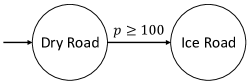
Figure 1: Hybrid adaptive cruise control system. The switching condition is when the position $p\geq 100$.

Scenario Setup. Adaptive cruise control (ACC) is a common example to validate safe control strategies [5, 37, 38], where the ego car and the leading car are driving on a straight road and the ego car is expected to maintain a safe distance with the leading car. In this case study, we consider ACC with hybrid dynamics following [10]. Specifically, the road is partitioned to high-friction part and low-friction part, which are called dry road and ice road, respectively, as shown in Figure 1. On the dry road, the dynamics is modelled as

$$\begin{bmatrix}\dot{p}\\ \dot{v}\\ \dot{d}\end{bmatrix}=\begin{bmatrix}v\\ -\frac{1}{m}F_{dry}(v)\\ v_{0}-v\end{bmatrix}+\begin{bmatrix}0\\ \frac{1}{m}\\ 0\end{bmatrix}u.$$ (13)

The system state is $x=[p\;v\;d]^{T}$, where $p$ is the ego car position, $v$ is the ego car velocity, and $d$ is the distance between the two cars. The leading car is driving with speed $v_{0}$. The control input $u$ is the acceleration with bound constraint $u\in[-mc_{d}g,mc_{d}g]$. The friction on dry road is $F_{dry}(v)=f_{0,d}v^{2}+f_{1,d}v+f_{2}$. The dynamic on the ice road is defined similarly with lower friction $F_{ice}(v)$ and control bound $[-mc_{i}g,mc_{i}g]$. The desired cruise speed is $v_{d}>v_{0}$.

In our simulation, we have the safety specification defined by the constraint function $c(x)=d-T_{h}v$, where $T_{h}$ is the look-ahead time. The local CBF used for dry road is $h_{dry}(x)=d-T_{h}v-\frac{(v_{0}-v)^{2}}{2c_{dry}g}$, and the local CBF used for ice road $h_{ice}(x)$ can be defined analogously by replacing $c_{dry}$ with $c_{ice}$. The control objective is that the ego car is expected to achieve the desired speed $v_{d}$ and to follow the leading car as close as possible. Specifically, the trajectory cost is defined as:

$$\texttt{Cost}=\int_{0}^{T}(0.01(v(t)-v_{d})^{2}+0.1(d(t)-T_{h}v(t))^{2})dt.$$ (14)

Training Details. The training consists of three stages. First, we train the network only using the loss term $h_{2}$ in (12), i.e., the network tries to fit the boundary condition of PDE at $t=0$ at the beginning phase. Then, we add loss term $h_{1}$ back and fit function $B_{\theta}$ gradually from $t=0$ to $t=T$, where $T$ is terminal time of neural network CBVF. Finally, we decrease the learning rate and train the network for the whole time interval $[0,T]$. Note that the terminal time $T$ of CBVF should be infinite theoretically, but it suffices to let $T$ be a finite time in practice, e.g., the pre-set maximum simulation/experiment time. These three phases’ training required approximately $1.5$ hour totally using PyTorch with a single GPU NVIDIA GeForce RTX3090. All states are normalized to $[-1,1]$ and time is scaled to $[-1,0]$. The training dataset is composed of 65K sampled states, among which 25K sampled states are close to the switching region between dry road and ice road in order to increase the approximation accuracy over this area.

Training Results. We show that our trained DNN can represent the PDE solution very accurately compared with the ground truth from [10]. The training results are presented in Figure 2. We compute the mean square error (MSE) over the position of ego car in Figure 2(a). Also, the calculated MSE over all dimensions is $1.9\times 10^{-3}$. Additionally, we show the unsafe volume error (UVE) and safe volume error (SVE) in Figure 2(b), in which UVE is the percentage volume of unsafe states that are considered safe by DNN and SVE is the percentage volume of safe states that are considered unsafe by DNN. We can observe that UVE is less than $0.1\%$ and SVE is less than $12\%$, which implies that our trained DNN is very safe but also a bit conservative. We numerically show that the performance degradation is actually slight soon. For more training results such as loss curve and examples of DNN value and ground truth, please direct to the Appendix.

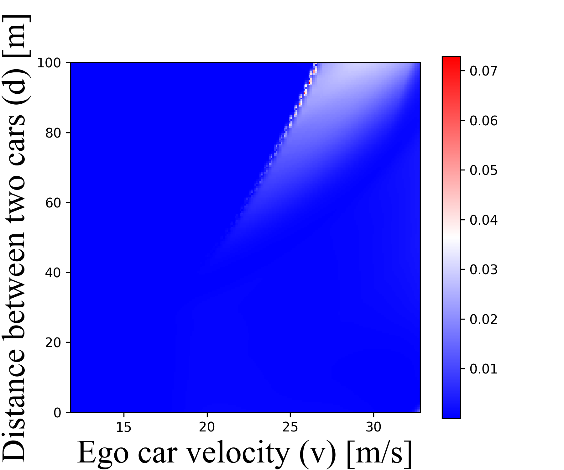
(a) MSE over position $p$

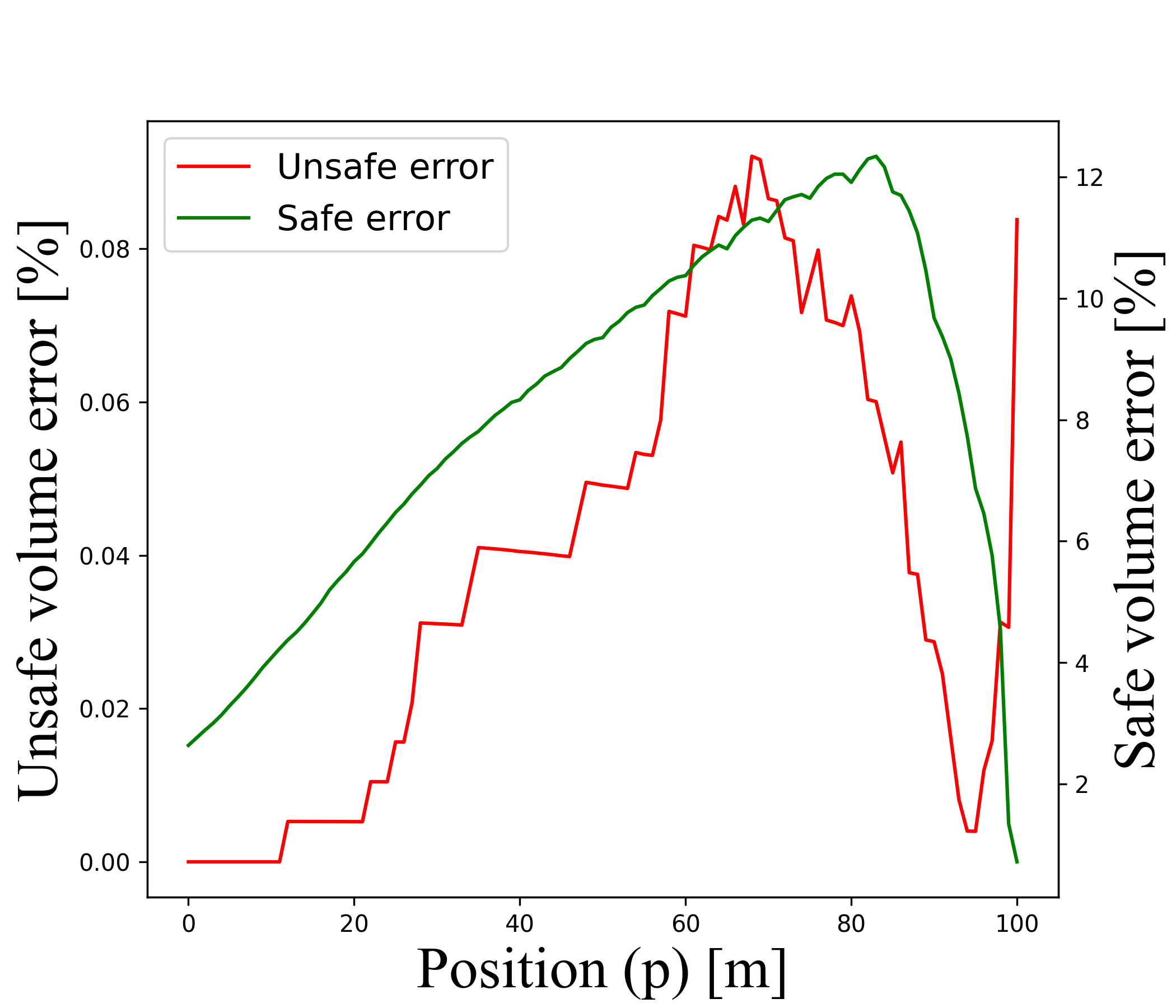
(b) Safe and unsafe volume errors

Figure 2: Training results of adaptive cruise control.

Numerical Comparison. We test four different baseline approaches over a horizon $T_{sim}=20s$ to evaluate their system performances. For CBF-based approaches, we choose a PID controller as the reference controller. For one testing initial condition $x(0)=[0\;30\;90]^{T}$, we plot all trajectories in Figure 3. Our numerical results are reported in Table I. We can observe that our neural switch-aware CBFs achieve very close performance to vanilla switch-aware CBFs [10], and it is even comparable with MPC. Switch-unaware local CBFs achieve reasonable performance but it violates hybrid system safety. Global CBF method is more conservative than local CBFs-based methods. In terms of online evaluation time, CBF-based approaches enjoy clear advantages over MPC. More details on parameters can be also found in Appendix.

(a) Neural switch-aware CBF

(b) Switch-aware CBF [10]

(c) Switch-unaware CBF

(d) Global CBF

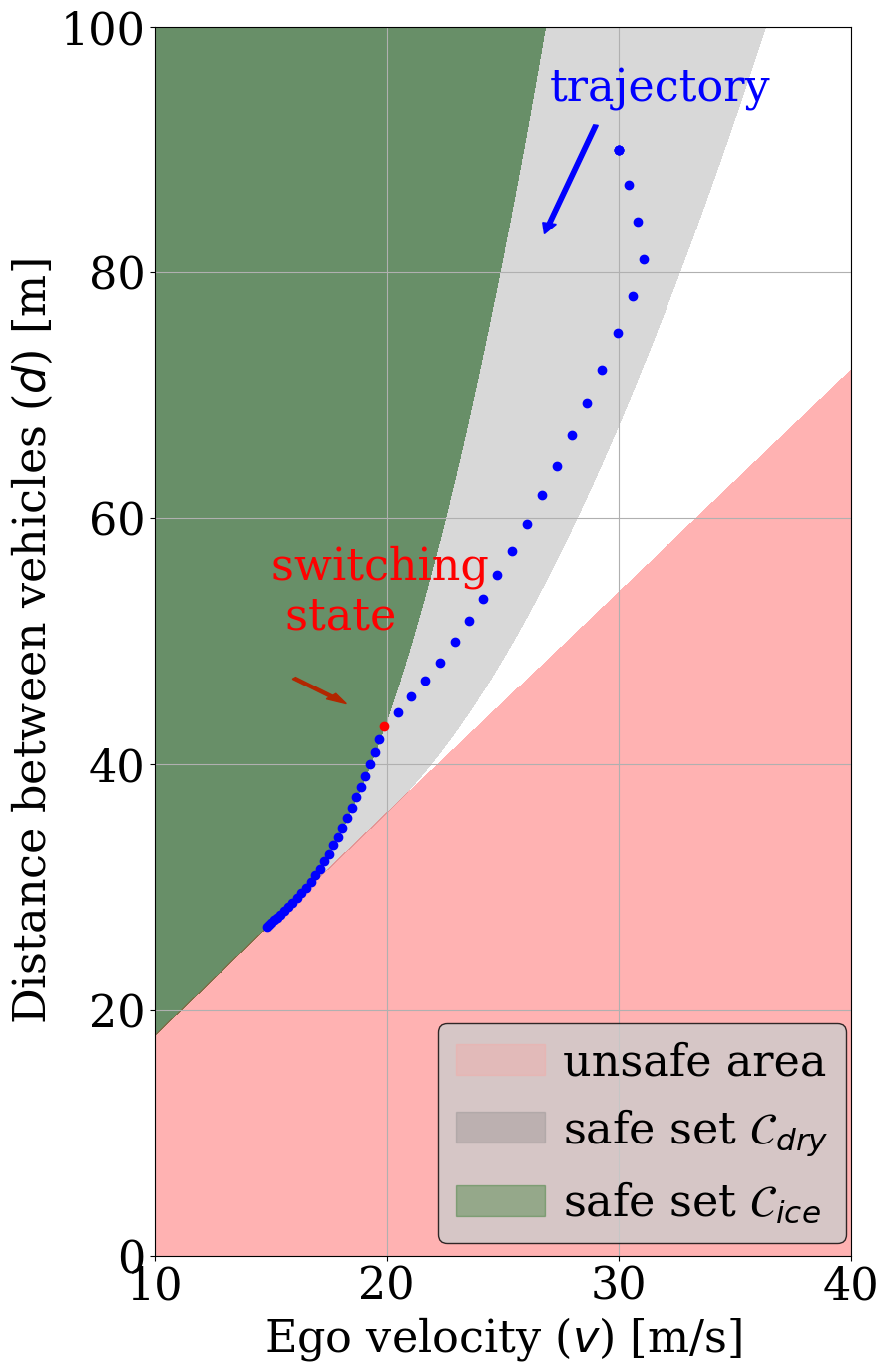
(e) MPC

Figure 3: Trajectories of our approach, original switch-aware CBF approach from [10], switch-unaware CBF approach, global CBF approach, and MPC. The unsafe area (red) is defined by the safety constraint function $c(x)$.

TABLE I: Closed-loop performance comparison of different methods in the adaptive cruise control example.

	Safety	Trajectory	Solve time
		cost	per step (s)
MPC	Safe	208.7	$1.7\!\times\!10^{-1}$
Global CBF	Safe	329.7	$5.6\!\times\!10^{-3}$
Switch-unaware CBFs	Unsafe	263.2	$5.7\!\times\!10^{-3}$
Switch-aware CBFs [10]	Safe	239.0	$5.7\!\times\!10^{-3}$
Neural switch-aware CBFs	Safe	244.8	$5.7\!\times\!10^{-3}$

IV-B 2D Autonomous Racing

Scenario Setup. We consider a second use case study using the F1Tenth gym simulator [39] with single-track model [40] (also known as the bicycle model). The state space model of single-track model is of 7 dimensions with two control inputs; the detailed dynamic equations of the model can be found in Appendix. Note that HJ-reach practically can only handle system with state dimension less than 6, so this case study cannot be addressed by approach in [10].

The racing track is a multi-friction road as shown in Figure 4. In this context, our safety specification is no collision with the wall. To ensure safety, we use a CBF from [41] at time $t$:

$$h_{wall}(x)=|e_{wall}-e_{t}|-\frac{\dot{e}_{t}^{2}}{a_{brake}}-d_{margin},$$ (15)

where $e_{wall}$ is the lateral distance with the wall from the track center-line, $e_{t}$ represents the lateral Frenet coordinate, $\dot{e}_{t}$ is its velocity, $a_{brake}$ is the maximum brake, and $d_{margin}$ is the safety margin. The intuition of $h_{wall}(x)$ is to define and ensure the safety as keeping the lateral coordinate within a safe margin $d_{margin}$ with the track boundaries. To consider the road friction, we replace the $a_{brake}$ term in (15) with $\eta\cdot a_{brake}$, where $\eta$ is a friction-dependent coefficient.

The control objective in this case study is to track a pre-computed optimal racing line [42] in the map and finish one lap while avoiding collision with the boundaries. For CBF-based approaches, we use pure pursuit and PID as our reference planner and controller respectively.

Training Details. We train two DNNs with three stages similar to the case of the ACC example. Here two DNNs are used for CBFs corresponding to the left and the right walls, respectively. More training details as well as the simulation parameters are available in Appendix.

Numerical Comparison. The simulation results are reported in Table II. Still, we can observe that vanilla switch-aware CBFs [10] is not applicable due to the high dimensionality of system state. MPC can finish one lap fastest while preserving safety, but its solving time per step is as high as almost 1 second. Our neural switch-aware CBFs performs close to MPC and the solving time is significantly lower. Global CBF is conservative regarding lap time and switch-unaware CBFs is not safe.

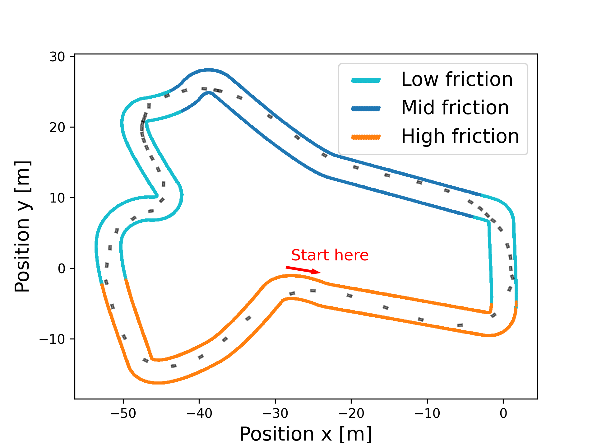
Figure 4: Multi-friction racing track. The trajectory from our approach is also presented.

TABLE II: Closed-loop performance comparison of controllers in the 2D autonomous racing example.

	Safety	Lap time	Solve time
		(s)	per step (s)
MPC	Safe	34.3	$7.2\times 10^{-1}$
Global CBF	Safe	69.2	$8.4\times 10^{-3}$
Switch-unaware CBFs	Unsafe	N/A	$8.2\times 10^{-3}$
Switch-aware CBFs [10]	N/A	N/A	N/A
Neural switch-aware CBFs	Safe	42.4	$8.0\times 10^{-3}$

V Conclusion and Discussion

In this work, we proposed a learning-enabled local CBFs method for safety control of hybrid systems. Specifically, we leveraged learning techniques to refine existing local CBFs, which are constructed without considering mode switchings, to ensure global safety. Our approach can scale to high-dimension systems and enjoys low computation cost during inference time. The proposed approach outperforms other safety-critical control methods, which is illustrated by two numerical simulations including one high-dimension autonomous racing case. In the future, we are interested in providing theoretical guarantees for the trained DNN to assure the validity of our neural CBFs. Also, we plan to conduct real-world experiments to validate our approach.

-A Experimental Details and Results

Adaptive Cruise Control. The training loss curve is shown in Figure 5(c). Figure 5(a) and Figure 5(b) are DNN and ground truth values when position ($p=95$) is around the switching area ($p=100$). We can observe that DNN can accurately recover the ground truth value. Parameters are shown in Table III. Note that the MPC horizon is 70 steps because this is almost the least steps number to ensure feasibility practically.

Autonomous Racing. The training procedure is similar to Adaptive Cruise Control case. Relevant parameters are shown in Table I. Also, 20 steps is almost the minimum horizon for MPC otherwise there is feasibility issue in practice.

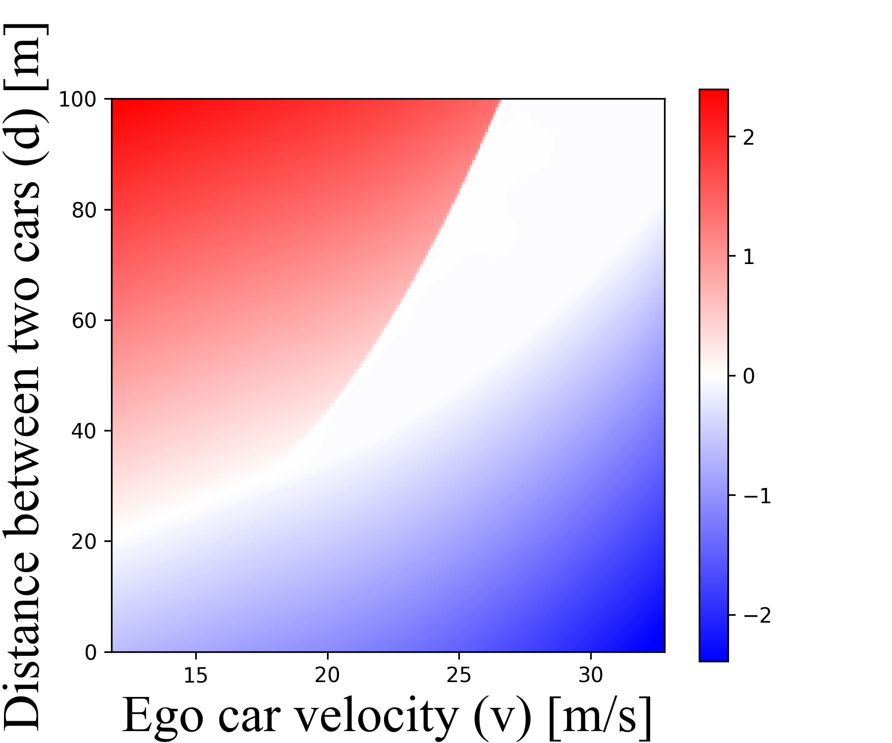
(a) DNN value for $p=95$

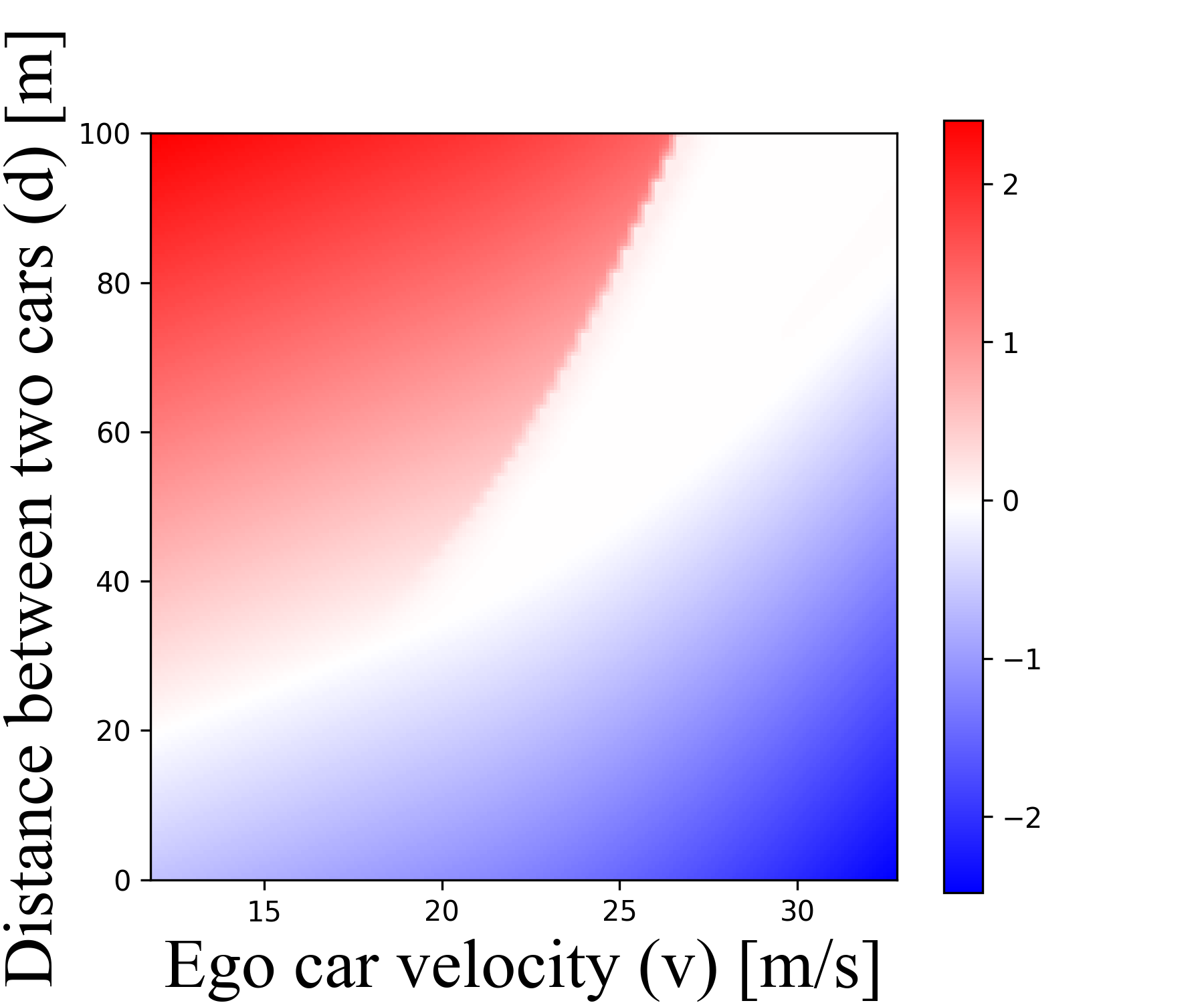
(b) Ground truth for $p=95$

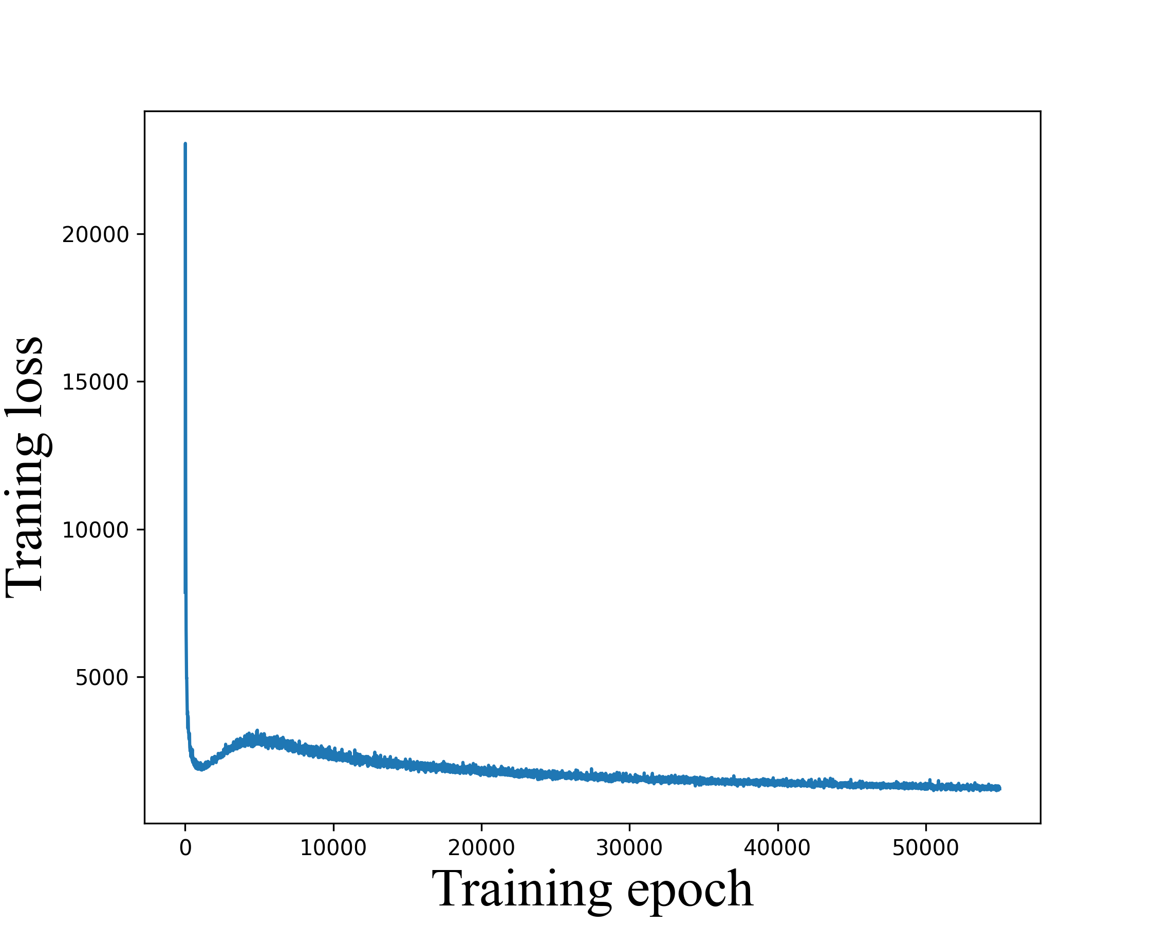
(c) Training loss curve

Figure 5: Training results of adaptive cruise control.

-B Single-Track Model

The single-track models a road vehicle with two wheels, where the front and rear wheel pairs are each lumped into one wheel. Compared with kinematic single-track mode, single-track model additionally considers tire slip, whose effect is more dominant when the vehicle is driving close to the physical capabilities. The state space model consist of 7 states $\mathbb{x}=\begin{bmatrix}s_{x}&s_{y}&\delta&v&\Psi&\dot{\Psi}&\beta\end{bmatrix}$ where the control input variables are $\begin{bmatrix}u_{1}&u_{2}\end{bmatrix}=\begin{bmatrix}v_{\delta}&a_{long}\end{bmatrix}.$

$$\dot{x}_{1}= x_{4}\cos\left(x_{5}+x_{7}\right),$$ (16)

$$\dot{x}_{2}= x_{4}\sin\left(x_{5}+x_{7}\right),$$

$$\dot{x}_{3}= f_{steer}\left(x_{3},u_{1}\right),$$

$$\dot{x}_{4}= f_{acc}\left(x_{4},u_{2}\right)$$

$$\dot{x}_{5}= x_{6},$$

$$\dot{x}_{6}= \frac{\mu m}{I_{z}\left(l_{r}+l_{f}\right)}(l_{f}C_{S,f}(gl_{r}-u_{2}h_{cg})x_{3}+(l_{r}C_{S,r}(gl_{f}$$

$$+u_{2}h_{cg})-l_{f}C_{S,f}(gl_{r}-u_{2}h_{cg}))x_{7}-(l_{f}^{2}C_{S,f}(gl_{r}$$

$$-u_{2}h_{cg})+l_{r}^{2}C_{S,r}(gl_{f}+u_{2}h_{cg}))\frac{x_{6}}{x_{4}}),$$

$$\dot{x}_{7}= \frac{\mu}{x_{4}(l_{r}+l_{f})}(C_{S,f}(gl_{r}-u_{2}h_{cg})x_{3}-(C_{S,r}(gl_{f}$$

$$+u_{2}h_{cg})+C_{S,f}(gl_{r}-u_{2}h_{cg}))x_{7}+(C_{S,r}(gl_{f}$$

$$+u_{2}h_{cg})l_{r}-C_{S,f}(gl_{r}-u_{2}h_{cg})l_{f})\frac{x_{6}}{x_{4}})-x_{6}.$$

where $f_{steer}$ and $f_{acc}$ impose physical constraints on steering and acceleration. Readers are referred to CommonRoad documentation [43] for the details of each parameter, which are omitted here due to limited space.

TABLE III: Adaptive cruise control (hyper)parameters.

Parameter	Value
Leading velocity $v_{0}$	14m/s
Desired velocity $v_{d}$	35m/s
Dry road friction coefficients $[f_{1}\;f_{2}\;f_{3}]$	$[0.3\ 15\ 0.75]$
Dry road control bound coefficient $c_{d}$	$0.3$
Ice road friction coefficients $[f_{1}\;f_{2}\;f_{3}]$	$[0.1\ 5\ 0.25]$
Ice road control bound coefficient $c_{i}$	$0.1$
Look-ahead time $T_{h}$	1.8s
MPC horizon	70 steps
MPC sampling frequency	10Hz
Simulation sampling frequency	100Hz
Simulation total time $T_{sim}$	20s
Neural network architecture	$[512\ 512\ 512]$
Neural network activation	Sine
Training optimizer	Adam
Learning rates	$2\times 10^{-5},8\times 10^{-7}$
Training epochs	5K,55K,5K
Terminal time $T$	25s

TABLE IV: Autonomous racing (hyper)parameters.

Parameter	Value
Friction coefficients $\mu_{low},\mu_{mid},\mu_{high}$	$0.12,0.6,1.04$
Friction brake coefficient $\eta_{low},\eta_{mid},\eta_{high}$	$0.01,50,500$
MPC horizon	20 steps
MPC sampling frequency	10Hz
Simulation sampling frequency	100Hz
Neural network architecture	$[512\ 512\ 512]$
Neural network activation	Sine
Training optimizer	Adam
Learning rates	$2\times 10^{-5},8\times 10^{-7}$
Training epochs for left wall	15K,165K,15K
Training epochs for right wall	25K,250K,25K
Terminal time $T$	20s

References

- [1] F. Borrelli, A. Bemporad, and M. Morari, Predictive control for linear and hybrid systems. Cambridge University Press, 2017.
- [2] C. J. Tomlin, I. Mitchell, A. M. Bayen, and M. Oishi, “Computational techniques for the verification of hybrid systems,” Proceedings of the IEEE, vol. 91, no. 7, pp. 986–1001, 2003.
- [3] S. Bansal, M. Chen, S. Herbert, and C. J. Tomlin, “Hamilton-jacobi reachability: A brief overview and recent advances,” in 2017 IEEE 56th Annual Conference on Decision and Control (CDC), pp. 2242–2253, IEEE, 2017.
- [4] B. Legat, P. Tabuada, and R. M. Jungers, “Computing controlled invariant sets for hybrid systems with applications to model-predictive control,” IFAC-PapersOnLine, vol. 51, no. 16, pp. 193–198, 2018.
- [5] A. D. Ames, X. Xu, J. W. Grizzle, and P. Tabuada, “Control barrier function based quadratic programs for safety critical systems,” IEEE Transactions on Automatic Control, vol. 62, no. 8, pp. 3861–3876, 2016.
- [6] A. D. Ames, S. Coogan, M. Egerstedt, G. Notomista, K. Sreenath, and P. Tabuada, “Control barrier functions: Theory and applications,” in 2019 18th European control conference (ECC), pp. 3420–3431, IEEE, 2019.
- [7] K.-C. Hsu, H. Hu, and J. F. Fisac, “The safety filter: A unified view of safety-critical control in autonomous systems,” arXiv preprint arXiv:2309.05837, 2023.
- [8] L. Lindemann, H. Hu, A. Robey, H. Zhang, D. Dimarogonas, S. Tu, and N. Matni, “Learning hybrid control barrier functions from data,” in Conference on Robot Learning, pp. 1351–1370, PMLR, 2021.
- [9] A. Robey, L. Lindemann, S. Tu, and N. Matni, “Learning robust hybrid control barrier functions for uncertain systems,” IFAC-PapersOnLine, vol. 54, no. 5, pp. 1–6, 2021.
- [10] S. Yang, M. Black, G. Fainekos, B. Hoxha, H. Okamoto, and R. Mangharam, “Safe control synthesis for hybrid systems through local control barrier functions,” arXiv preprint arXiv:2311.17201, 2023. Accepted by 2024 American Control Conference (ACC).
- [11] S. Bansal and C. J. Tomlin, “Deepreach: A deep learning approach to high-dimensional reachability,” in 2021 IEEE International Conference on Robotics and Automation (ICRA), pp. 1817–1824, IEEE, 2021.
- [12] J. Sirignano and K. Spiliopoulos, “Dgm: A deep learning algorithm for solving partial differential equations,” Journal of computational physics, vol. 375, pp. 1339–1364, 2018.
- [13] J. Han, A. Jentzen, and W. E, “Solving high-dimensional partial differential equations using deep learning,” Proceedings of the National Academy of Sciences, vol. 115, no. 34, pp. 8505–8510, 2018.
- [14] J. Berg and K. Nyström, “A unified deep artificial neural network approach to partial differential equations in complex geometries,” Neurocomputing, vol. 317, pp. 28–41, 2018.
- [15] M. Srinivasan, A. Dabholkar, S. Coogan, and P. A. Vela, “Synthesis of control barrier functions using a supervised machine learning approach,” in 2020 IEEE/RSJ International Conference on Intelligent Robots and Systems (IROS), pp. 7139–7145, IEEE, 2020.
- [16] A. Robey, H. Hu, L. Lindemann, H. Zhang, D. V. Dimarogonas, S. Tu, and N. Matni, “Learning control barrier functions from expert demonstrations,” in 2020 59th IEEE Conference on Decision and Control (CDC), pp. 3717–3724, IEEE, 2020.
- [17] A. Abate, D. Ahmed, A. Edwards, M. Giacobbe, and A. Peruffo, “Fossil: a software tool for the formal synthesis of lyapunov functions and barrier certificates using neural networks,” in Proceedings of the 24th International Conference on Hybrid Systems: Computation and Control, pp. 1–11, 2021.
- [18] Z. Qin, K. Zhang, Y. Chen, J. Chen, and C. Fan, “Learning safe multi-agent control with decentralized neural barrier certificates,” arXiv preprint arXiv:2101.05436, 2021.
- [19] Y. Wang, S. S. Zhan, R. Jiao, Z. Wang, W. Jin, Z. Yang, Z. Wang, C. Huang, and Q. Zhu, “Enforcing hard constraints with soft barriers: Safe reinforcement learning in unknown stochastic environments,” in International Conference on Machine Learning, pp. 36593–36604, PMLR, 2023.
- [20] J. J. Choi, D. Lee, K. Sreenath, C. J. Tomlin, and S. L. Herbert, “Robust control barrier–value functions for safety-critical control,” in 2021 60th IEEE Conference on Decision and Control (CDC), pp. 6814–6821, IEEE, 2021.
- [21] P. Mhaskar, N. H. El-Farra, and P. D. Christofides, “Robust hybrid predictive control of nonlinear systems,” Automatica, vol. 41, no. 2, pp. 209–217, 2005.
- [22] M. Benerecetti, M. Faella, and S. Minopoli, “Automatic synthesis of switching controllers for linear hybrid systems: Safety control,” Theoretical Computer Science, vol. 493, pp. 116–138, 2013.
- [23] R. Ivanov, J. Weimer, R. Alur, G. J. Pappas, and I. Lee, “Verisig: verifying safety properties of hybrid systems with neural network controllers,” in Proceedings of the 22nd ACM International Conference on Hybrid Systems: Computation and Control, pp. 169–178, 2019.
- [24] D. Phan, N. Paoletti, T. Zhang, R. Grosu, S. A. Smolka, and S. D. Stoller, “Neural state classification for hybrid systems,” in Proceedings of the Fifth International Workshop on Symbolic-Numeric Methods for Reasoning About CPS and IoT, pp. 24–27, 2019.
- [25] S. Prajna and A. Jadbabaie, “Safety verification of hybrid systems using barrier certificates,” in International Workshop on Hybrid Systems: Computation and Control, pp. 477–492, Springer, 2004.
- [26] P. Glotfelter, I. Buckley, and M. Egerstedt, “Hybrid nonsmooth barrier functions with applications to provably safe and composable collision avoidance for robotic systems,” IEEE Robotics and Automation Letters, vol. 4, no. 2, pp. 1303–1310, 2019.
- [27] M. Maghenem and R. G. Sanfelice, “Characterizations of safety in hybrid inclusions via barrier functions,” in Proceedings of the 22nd ACM International Conference on Hybrid Systems: Computation and Control, pp. 109–118, 2019.
- [28] A. Nejati, S. Soudjani, and M. Zamani, “Compositional construction of control barrier functions for continuous-time stochastic hybrid systems,” Automatica, vol. 145, p. 110513, 2022.
- [29] R. Goebel, R. G. Sanfelice, and A. R. Teel, “Hybrid dynamical systems,” IEEE control systems magazine, vol. 29, no. 2, pp. 28–93, 2009.
- [30] S. Tonkens and S. Herbert, “Refining control barrier functions through hamilton-jacobi reachability,” in 2022 IEEE/RSJ International Conference on Intelligent Robots and Systems (IROS), pp. 13355–13362, IEEE, 2022.
- [31] V. Sitzmann, J. Martel, A. Bergman, D. Lindell, and G. Wetzstein, “Implicit neural representations with periodic activation functions,” Advances in neural information processing systems, vol. 33, pp. 7462–7473, 2020.
- [32] L. Lu, X. Meng, Z. Mao, and G. E. Karniadakis, “Deepxde: A deep learning library for solving differential equations,” SIAM review, vol. 63, no. 1, pp. 208–228, 2021.
- [33] A. Lin and S. Bansal, “Generating formal safety assurances for high-dimensional reachability,” in 2023 IEEE International Conference on Robotics and Automation (ICRA), pp. 10525–10531, IEEE, 2023.
- [34] G. C. Calafiore and M. C. Campi, “The scenario approach to robust control design,” IEEE Transactions on automatic control, vol. 51, no. 5, pp. 742–753, 2006.
- [35] Y. Chen, C. Shang, X. Huang, and X. Yin, “Data-driven safe controller synthesis for deterministic systems: A posteriori method with validation tests,” arXiv preprint arXiv:2304.00729, 2023.
- [36] J. A. Andersson, J. Gillis, G. Horn, J. B. Rawlings, and M. Diehl, “Casadi: a software framework for nonlinear optimization and optimal control,” Mathematical Programming Computation, vol. 11, pp. 1–36, 2019.
- [37] J. Zeng, B. Zhang, Z. Li, and K. Sreenath, “Safety-critical control using optimal-decay control barrier function with guaranteed point-wise feasibility,” in 2021 American Control Conference (ACC), pp. 3856–3863, IEEE, 2021.
- [38] S. Yang, S. Chen, V. M. Preciado, and R. Mangharam, “Differentiable safe controller design through control barrier functions,” IEEE Control Systems Letters, vol. 7, pp. 1207–1212, 2022.
- [39] M. O’Kelly, H. Zheng, D. Karthik, and R. Mangharam, “F1tenth: An open-source evaluation environment for continuous control and reinforcement learning,” Proceedings of Machine Learning Research, vol. 123, 2020.
- [40] M. Althoff, M. Koschi, and S. Manzinger, “Commonroad: Composable benchmarks for motion planning on roads,” in 2017 IEEE Intelligent Vehicles Symposium (IV), pp. 719–726, IEEE, 2017.
- [41] L. Berducci, S. Yang, R. Mangharam, and R. Grosu, “Learning adaptive safety for multi-agent systems,” arXiv preprint arXiv:2309.10657, 2023.
- [42] A. Heilmeier, A. Wischnewski, L. Hermansdorfer, J. Betz, M. Lienkamp, and B. Lohmann, “Minimum curvature trajectory planning and control for an autonomous race car,” Vehicle System Dynamics, 2019.
- [43] “Commonroad documentation.” https://gitlab.lrz.de/tum-cps/commonroad-vehicle-models.