Convergence analysis of the adaptive stochastic collocation finite element method

Abstract.

This paper is focused on the convergence analysis of an adaptive stochastic collocation algorithm for the stationary diffusion equation with parametric coefficient. The algorithm employs sparse grid collocation in the parameter domain alongside finite element approximations in the spatial domain, and adaptivity is driven by recently proposed parametric and spatial a posteriori error indicators. We prove that for a general diffusion coefficient with finite-dimensional parametrization, the algorithm drives the underlying error estimates to zero. Thus, our analysis covers problems with affine and nonaffine parametric coefficient dependence.

1. Introduction

Sparse grid stochastic collocation is an established and well-studied computational method for solving high-dimensional parametric partial differential equations (PDEs) that are ubiquitous in uncertainty quantification models. The sparsity of the underlying set of collocation points is critical for this task even for moderately high-dimensional problems, as basic tensor-product grids of collocation points yield approximations suffering from the curse of dimensionality; see, for example, [BNT07, NTW08b, NTW08a, Bie11, BTNT12, NTT16, EST18]. Furthermore, in a typical setting of a high-dimensional parametric PDE, the solution is anisotropic in the parameter domain, calling for adaptive enrichment of sparse grid collocation points.

Adaptively generated sparse grids trace back to the work of Gerstner and Griebel [GG03] on high-dimensional quadratures. Their ideas have found successful applications to collocation methods for parametric PDEs, see, for example, [CCS14, NTTT16], where parametric adaptivity is driven by heuristic error indicators that require solving additional PDEs. An alternative approach, proposed in [GN18], is based on a posteriori error estimation. Here, a reliable residual-based a posteriori error estimator is derived to control two distinct sources of discretization error arising from parametric (sparse grid collocation) and spatial (finite element) components of approximations. Crucially, this error estimator avoids the solution of additional PDEs; it is also localizable and, thus, can be readily used in an adaptive algorithm. In particular, the parametric component of the error estimator is used in [GN18] to design an algorithm that generates adaptive sparse grid (semidiscrete) approximations. The convergence analysis of a modified version of the adaptive algorithm in [GN18] is performed in [EEST22]. In [FS21], the authors extended the adaptive algorithm proposed in [GN18] to include spatial (finite element) adaptivity and proved convergence of the resulting ‘fully adaptive’ algorithm.

It is important to note that the a posteriori error estimation framework developed in [GN18] and, hence, the adaptive algorithms in [GN18, EEST22, FS21], are inherently restricted to parametric PDEs whose inputs have affine dependence on parameters; cf. [GN18, section 4]. In our recent work [BSX22], we proposed a novel a posteriori error estimation strategy for finite element-based sparse grid stochastic collocation approximations. This error estimation strategy is applicable to general elliptic parametric PDEs with either affine or nonaffine parametric dependence of inputs. It is similar in spirit to the hierarchical error estimation framework proposed in the context of stochastic Galerkin finite element methods, see [BPS14, BS16, BPRR19a, BPRR19b, BX20].

In this contribution, we bridge a gap in the existing theory of adaptive algorithms for stochastic collocation finite element methods (SC-FEMs) by extending the convergence analysis in [EEST22, FS21] to a broader class of parametric elliptic PDEs that covers problems with nonaffine parametric coefficients. Specifically, we study convergence of an adaptive algorithm guided by reliable a posteriori error estimates and the associated error indicators proposed in [BSX22]. We note that the adaptive algorithm considered in this work is slightly different from the one proposed in [BSX22]; the difference lies in how the algorithm performs parametric marking and enrichment (see Remark 7). Our main result in Theorem 14 shows that the modified adaptive algorithm generates SC-FEM approximations, with the corresponding sequence of error estimates converging to zero. A key ingredient of our analysis is a certain summability property of Taylor coefficients for semidiscrete (finite element) approximations. We prove that this summability property holds in the case of affine-parametric coefficients satisfying the uniform ellipticity assumption (see Lemma 1). Furthermore, for PDEs with general parametric coefficients, we show that the assumptions guaranteeing the analyticity of the exact solution in the parameter domain also ensure the required summability property of Taylor coefficients for semidiscrete approximations (see Lemma 2 and Remark 3).

The outline of the paper is as follows. After introducing the parametric model problem in section 2, we set up its stochastic collocation discretization in section 3. Section 4 focuses on the summability property of Taylor coefficients for semidiscrete (finite element) approximations. In section 5, we recall the main components of the a posteriori error estimation strategy developed in [BSX22] and present the adaptive SC-FEM algorithm. Sections 6 and 7 focus on proving convergence of parametric and spatial error estimates for SC-FEM approximations generated by the adaptive algorithm. In section 8, we formulate and prove the main result of this work. The results of numerical experiments are presented and discussed in section 9.

2. Parametric model problem

Let $D\subset\mathbb{R}^{2}$ be a bounded Lipschitz domain with polygonal boundary $\partial D$; we will refer to $D$ as the spatial domain. Let us also introduce the parameter domain $\Gamma:=\Gamma_{1}\times\Gamma_{2}\ldots\times\Gamma_{M}\subset\mathbb{R}^{M}$, where $M\in\mathbb{N}$ and each $\Gamma_{m}$ ($m=1,\ldots,M$) is a bounded interval in $\mathbb{R}$. Let $\pi(\mathbf{y}):=\prod_{m=1}^{M}\pi_{m}(y_{m})$ be a probability measure on $(\Gamma,\mathcal{B}(\Gamma))$; here, $\mathcal{B}(\Gamma)$ is the Borel $\sigma$-algebra on $\Gamma$, and $\pi_{m}$ denotes a probability measure on $(\Gamma_{m},\mathcal{B}(\Gamma_{m}))$ for $m=1,\ldots,M$.

We consider the following parametric elliptic problem: find $u:\overline{D}\times\Gamma\to\mathbb{R}$ satisfying

$$-\nabla\cdot(a(\cdot,\mathbf{y})\nabla u(\cdot,\mathbf{y})) =f \text{in $D$},$$ (1)

$$u(\cdot,\mathbf{y}) =0 \partial D$$ on

$\pi$-almost everywhere on $\Gamma$ (i.e., almost surely). Here, the forcing term $f\in L^{2}(D)$ is deterministic and the coefficient $a$ is a random field on $(\Gamma,\mathcal{B}(\Gamma),\pi)$ over $L^{\infty}(D)$. We assume that the coefficient $a$ is positive and bounded, i.e.,

$$0<a_{\min}\leq\operatorname*{ess\;inf}_{x\in D}a(x,\mathbf{y})\leq\operatorname*{ess\;sup}_{x\in D}a(x,\mathbf{y})\leq a_{\max}<\infty\quad\text{$\pi$-a.e. on $\Gamma$}$$ (2)

with some positive constants $a_{\min}$, $a_{\max}$. This assumption implies the norm equivalence for the Sobolev space on the spatial domain: for any $v\in\mathbb{X}:=H^{1}_{0}(D)$ there holds

$$a_{\min}\|\nabla v\|_{L^{2}(D)}^{2}\leq\|a(\cdot,\mathbf{y})\nabla v\|_{L^{2}(D)}^{2}\leq a_{\max}\|\nabla v\|_{L^{2}(D)}^{2}\quad\text{$\pi$-a.e. on $\Gamma$}.$$ (3)

For the purpose of finding the numerical solution to the parametric problem (1), we write it in the following weak form: given $f\in L^{2}(D)$, find $u:\Gamma\to\mathbb{X}$ such that

$$\int_{D}a(x,\mathbf{y})\nabla u(x,\mathbf{y})\cdot\nabla v(x)\mathrm{d}x=\int_{D}f(x)v(x)\mathrm{d}x\quad\forall v\in\mathbb{X},\ \text{$\pi$-a.e. on $\Gamma$}.$$ (4)

The above assumptions on the problem data ensure the existence and uniqueness of the solution $u$ in the Bochner space $\mathbb{V}:=L_{\pi}^{p}(\Gamma;\mathbb{X})$ for any $p\in[1,\infty]$; see [BNT07, Lemma 1.1] for details.

3. Stochastic collocation finite element method

For the numerical solution of problem (1) we apply the stochastic collocation finite element method. Let us recall the main ideas, including the construction of the underlying approximation spaces.

We denote by $\mathcal{T}_{\bullet}$ a mesh on the spatial domain $D$ (i.e., a conforming triangulation of $D$ into compact non-degenerate triangles $T$) and let $\mathcal{N}_{\bullet}$ denote the set of vertices of $\mathcal{T}_{\bullet}$. For mesh refinement, we employ newest vertex bisection (NVB); see, e.g., [Ste08, KPP13]. We assume that any mesh $\mathcal{T}_{\bullet}$ employed for the spatial discretization is obtained by (uniform or local) refinement of a given (coarse) initial mesh $\mathcal{T}_{0}$. For the numerical solution of (4), we employ the space $\mathbb{X}_{\bullet}$ of continuous piecewise linear functions,

$$\mathbb{X}_{\bullet}:=\SS^{1}_{0}(\mathcal{T}_{\bullet}):=\{v\in\mathbb{X}:v|_{T}\text{ is affine for all }T\in\mathcal{T}_{\bullet}\}\subset\mathbb{X}=H^{1}_{0}(D).$$

In particular, $\mathbb{X}_{0}:=\SS^{1}_{0}(\mathcal{T}_{0}).$ The standard basis of $\mathbb{X}_{\bullet}$ is given by $\{\varphi_{\bullet,\xi}:\xi\in\mathcal{N}_{\bullet}\setminus\partial D\}$, where $\varphi_{\bullet,\xi}$ denotes the hat function associated with the vertex $\xi\in\mathcal{N}_{\bullet}$.

Let $\widehat{\mathcal{T}}_{\bullet}$ be the mesh obtained by uniform NVB refinement of $\mathcal{T}_{\bullet}$ (i.e., all elements in $\mathcal{T}_{\bullet}$ are refined by three bisections). Then, $\widehat{\mathcal{N}}_{\bullet}$ denotes the set of vertices of $\widehat{\mathcal{T}}_{\bullet}$, and $\mathcal{N}_{\bullet}^{+}:=(\widehat{\mathcal{N}}_{\bullet}\setminus\mathcal{N}_{\bullet})\setminus\partial D$ is the set of new interior vertices created by this refinement of $\mathcal{T}_{\bullet}$. The finite element space associated with $\widehat{\mathcal{T}}_{\bullet}$ is denoted as $\widehat{\mathbb{X}}_{\bullet}:=\SS^{1}_{0}(\widehat{\mathcal{T}}_{\bullet})$, and $\{\widehat{\varphi}_{\bullet,\xi}:\xi\in\widehat{\mathcal{N}}_{\bullet}\setminus\partial D\}$ is the corresponding basis of hat functions.

Let $\mathbf{z}$ be a fixed point in $\Gamma$. We denote by $u_{\bullet\mathbf{z}}\in\mathbb{X}_{\bullet}$ the Galerkin finite element approximation satisfying

$$\int_{D}a(x,\mathbf{z})\nabla u_{\bullet\mathbf{z}}(x)\cdot\nabla v(x)\mathrm{d}x=\int_{D}f(x)v(x)\mathrm{d}x\quad\forall v\in\mathbb{X}_{\bullet}.$$ (5)

Hence, given a finite set $\mathcal{Y}_{\bullet}$ of collocation points in $\Gamma$, the SC-FEM approximation of the solution $u$ to parametric problem (1) is given by

$$u_{\bullet}^{\rm SC}(x,\mathbf{y}):=\sum\limits_{\mathbf{z}\in\mathcal{Y}_{\bullet}}u_{\bullet\mathbf{z}}(x)L_{\bullet\mathbf{z}}(\mathbf{y}),$$ (6)

where $\{L_{\bullet\mathbf{z}}(\mathbf{y}),\mathbf{z}\in\mathcal{Y}_{\bullet}\}$ is a set of multivariable Lagrange basis functions constructed for the set of collocation points $\mathcal{Y}_{\bullet}$ and satisfying $L_{\bullet\mathbf{z}}(\mathbf{z}^{\prime})=\delta_{\mathbf{z}\mathbf{z}^{\prime}}$, $\forall\mathbf{z},\,\mathbf{z}^{\prime}\in\mathcal{Y}_{\bullet}$.

Note that the SC-FEM solution considered in this work follows the so-called single-level construction that employs the same finite element space $\mathbb{X}_{\bullet}$ for all collocation points $\mathbf{z}\in\mathcal{Y}_{\bullet}$ (cf. [BNT07, NTW08b, GN18, BSX22]). This is in contrast to the multilevel SC-FEM approximations that allow $\mathbb{X}_{\bullet\mathbf{z}}\not=\mathbb{X}_{\bullet\mathbf{z}^{\prime}}$ for $\mathbf{z}\not=\mathbf{z}^{\prime}$; see, e.g., [LSS20, FS21, BS23].

In the context of the numerical solution of high-dimensional parametric problems, the state-of-the-art stochastic collocation methods employ the nodes of sparse grids as collocation points. We briefly describe the construction of sparse grids in the next section.

3.1. Sparse grid interpolation

Since any finite interval in $\mathbb{R}$ can be mapped to $[-1,1]$ via appropriate linear transformation, we can assume without loss of generality that $\Gamma_{1}=\Gamma_{2}=\ldots=\Gamma_{M}=[-1,1]$. The construction of a sparse grid $\mathcal{Y}_{\bullet}\subset\Gamma=[-1,1]^{M}$ hinges on three ingredients:

• a family of nested sets of 1D nodes on $[-1,1]$ (in this work, we will consider the nested sets of Leja points and Clenshaw–Curtis (CC) quadrature points);

• a strictly increasing function $\kappa:\mathbb{N}_{0}\to\mathbb{N}_{0}$ satisfying $\kappa(0)=0$, $\kappa(1)=1$ (e.g., $\kappa(i)=i$ for Leja points and $\kappa(i)=2^{i-1}+1$, $i>1$ for CC nodes with the doubling rule).

• a monotone finite set $\Lambda_{\bullet}\,{\subset}\,\mathbb{N}^{M}$ of multi-indices; specifically, $\Lambda_{\bullet}\,{=}\,\{\boldsymbol{\nu}\,{=}\,[\nu_{1},\ldots,\nu_{M}]:\nu_{m}\in\mathbb{N},\,m=1,\ldots,M\}$ is such that $\#\Lambda_{\bullet}<\infty$ and

  $$\boldsymbol{\nu}\in\Lambda_{\bullet}\Longrightarrow\boldsymbol{\nu}-\boldsymbol{\varepsilon}_{m}\in\Lambda_{\bullet}\quad\forall\,m=1,\ldots,M\text{ such that }\nu_{m}>1,$$

  where $(\boldsymbol{\varepsilon}_{m})_{i}=\delta_{mi}$ for all $i=1,\ldots,M$. Note that the monotonicity property of $\Lambda_{\bullet}$ implies that $\boldsymbol{1}=[1,1,\dots,1]\in\Lambda_{\bullet}$;

Now, for each $\boldsymbol{\nu}\in\Lambda_{\bullet}$, the set of nodes along the $m$-th coordinate axis in $\mathbb{R}^{M}$ is given by the set $\mathcal{Y}_{m}^{\kappa(\nu_{m})}$ such that $\#\mathcal{Y}_{m}^{\kappa(\nu_{m})}=\kappa(\nu_{m})$, and we define

$$\mathcal{Y}^{\,(\boldsymbol{\nu})}:=\mathcal{Y}_{1}^{\kappa(\nu_{1})}\times\mathcal{Y}_{2}^{\kappa(\nu_{2})}\times\ldots\times\mathcal{Y}_{M}^{\kappa(\nu_{M})}.$$

For a given index set $\Lambda_{\bullet}$, the sparse grid $\mathcal{Y}_{\bullet}$ of collocation points on $\Gamma$ is defined as

$$\mathcal{Y}_{\bullet}=\mathcal{Y}_{\Lambda_{\bullet}}:=\bigcup_{\boldsymbol{\nu}\in\Lambda_{\bullet}}\mathcal{Y}^{\,(\boldsymbol{\nu})}.$$

Let $I_{m}^{\kappa(\nu_{m})}:C^{0}([-1,1];\mathbb{X})\to\mathbb{P}_{\kappa(\nu_{m})-1}([-1,1];\mathbb{X})$ be the standard Lagrange interpolation operator associated with the set of 1D nodes $\mathcal{Y}_{m}^{\kappa(\nu_{m})}\subset[-1,1]$. Here, $\mathbb{P}_{q}$ is the set of univariate polynomials of degree at most $q\in\mathbb{N}_{0}$. Setting $I_{m}^{0}=0$ for all $m=1,\ldots,M$, we define 1D detail operators

$$\Delta_{m}^{\kappa(\nu_{m})}:=I_{m}^{\kappa(\nu_{m})}-I_{m}^{\kappa(\nu_{m}-1)}.$$

Now, the sparse grid collocation operator associated with the sparse grid $\mathcal{Y}_{\Lambda_{\bullet}}$ is defined as

$$S_{\bullet}=S_{\Lambda_{\bullet}}:=\sum\limits_{\boldsymbol{\nu}\in\Lambda_{\bullet}}\Delta^{\boldsymbol{\kappa}(\boldsymbol{\nu})},$$ (7)

where $\boldsymbol{\kappa}(\boldsymbol{\nu}):=[\kappa(\nu_{1}),\ldots,\kappa(\nu_{M})]$ and $\Delta^{\boldsymbol{\kappa}(\boldsymbol{\nu})}:=\bigotimes_{m=1}^{M}\Delta_{m}^{\kappa(\nu_{m})}$ is called the hierarchical surplus operator.

The nestedness of 1D node sets and the monotonicity of the index set $\Lambda_{\bullet}$ ensure the interpolation property for the operator $S_{\Lambda_{\bullet}}$ (cf. [BNTT11]), i.e.,

$$S_{\Lambda_{\bullet}}:C^{0}(\Gamma;\mathbb{X})\to\mathbb{P}_{\Lambda_{\bullet}}(\Gamma;\mathbb{X})\text{\; is such that \;}S_{\Lambda_{\bullet}}v(\mathbf{z})=v(\mathbf{z})\ \;\forall\,\mathbf{z}\in\mathcal{Y}_{\Lambda_{\bullet}},$$ (8)

where $\mathbb{P}_{\Lambda_{\bullet}}:=\bigoplus_{\boldsymbol{\nu}\in\Lambda_{\bullet}}\mathbb{P}_{\boldsymbol{\kappa}(\boldsymbol{\nu})-\boldsymbol{1}}$ with $\mathbb{P}_{\boldsymbol{\kappa}(\boldsymbol{\nu})-\boldsymbol{1}}:=\bigotimes_{m=1}^{M}\mathbb{P}_{\kappa(\nu_{m})-1}$. Therefore, the SC-FEM solution defined by (6) can be written as

$$u_{\bullet}^{\rm SC}(x,\mathbf{y})=[S_{\bullet}U_{\bullet}](x,\mathbf{y})=\sum\limits_{\mathbf{z}\in\mathcal{Y}_{\bullet}}u_{\bullet\mathbf{z}}(x)L_{\bullet\mathbf{z}}(\mathbf{y})$$ (9)

with a function $U_{\bullet}:\Gamma\to\mathbb{X}_{\bullet}$ satisfying $U_{\bullet}(\mathbf{z})=u_{\bullet\mathbf{z}}$ for all $\mathbf{z}\in\mathcal{Y}_{\bullet}$.

Let $\mathbb{W}\in\big{\{}\mathbb{X}_{0},\mathbb{X}_{\bullet},\widehat{\mathbb{X}}_{\bullet}\big{\}}$. We introduce a semidiscrete approximation $w:\Gamma\to\mathbb{W}$ such that $w(\cdot,\mathbf{y})\in\mathbb{W}$ satisfies

$$\int_{D}a(x,\mathbf{y})\nabla w(x,\mathbf{y})\cdot\nabla v(x)\mathrm{d}x=\int_{D}f(x)v(x)\mathrm{d}x\quad\forall v\in\mathbb{W},\ \text{$\pi$-a.e. in $\Gamma$}$$ (10)

(for each $\mathbb{W}\in\big{\{}\mathbb{X}_{0},\mathbb{X}_{\bullet},\widehat{\mathbb{X}}_{\bullet}\big{\}}$, the corresponding semidiscrete approximation satisfying (10) will be denoted by $u_{0}^{\rm semi},\,u_{\bullet}^{\rm semi}$ and $\hat{u}_{\bullet}^{\rm semi}$, respectively). We assume that the following two representations of $w$ hold (cf. [GN18, eq. (12)]):

$$w(x,\mathbf{y}):=\sum\limits_{\mathbf{i}\in\mathbb{N}_{0}^{M}}w_{\mathbf{i}}(x)P_{\mathbf{i}}(\mathbf{y})=\sum\limits_{\boldsymbol{\nu}\in\mathbb{N}^{M}}\Delta^{\boldsymbol{\kappa}(\boldsymbol{\nu})}w(x,\mathbf{y})\quad\text{$\pi$-a.e. on $\Gamma$},$$ (11)

where $P_{\mathbf{i}}(\mathbf{y})=\prod_{m=1}^{M}y_{m}^{i_{m}}$ and

$$w_{\mathbf{i}}(x)=\frac{1}{\mathbf{i}!}\frac{\partial^{\mathbf{i}}w(x,\mathbf{y})}{\partial\mathbf{y}^{\mathbf{i}}}\Big{|}_{\mathbf{y}=\boldsymbol{0}},\quad\mathbf{i}\in\mathbb{N}^{M}_{0}$$ (12)

are the Taylor coefficients. The following summability property of the Taylor coefficients $w_{\mathbf{i}}(x)$ will play a key role in our analysis: there exists $\boldsymbol{\rho}=[\rho_{1},\dots,\rho_{M}]>\boldsymbol{1}$ such that

$$\left(\boldsymbol{\rho}^{\mathbf{i}}\big{\|}w_{\mathbf{i}}\big{\|}_{\mathbb{X}}\right)_{\mathbf{i}\in\mathbb{N}_{0}^{M}}\in l^{2}(\mathbb{N}_{0}^{M})\quad\text{and}\quad\sum\limits_{\mathbf{i}\in\mathbb{N}_{0}^{M}}\boldsymbol{\rho}^{2\mathbf{i}}\big{\|}w_{\mathbf{i}}\big{\|}^{2}_{\mathbb{X}}\leq C<\infty,$$ (13)

where $C$ is independent of the underlying finite element space. Hereafter, for two vectors $\mathbf{a}=[a_{1},\ldots,a_{M}]\in\mathbb{R}^{M}$ and $\mathbf{b}=[b_{1},\ldots,b_{M}]\in\mathbb{R}^{M}$, we use the notation $\mathbf{a}^{\mathbf{b}}:=\prod_{m=1}^{M}a_{m}^{b_{m}}$ and $\mathbf{a}\mathbf{b}:=\prod_{m=1}^{M}a_{m}b_{m}$; we also write $\mathbf{a}>\mathbf{b}$ iff $a_{m}>b_{m}$ for all $m=1,\dots,M$; furthermore, for $\mathbf{i}\in\mathbb{N}_{0}^{M}$, we denote by $\mathbf{i}!=\prod_{m=1}^{M}i_{m}!$ the multivariable factorial.

In the next section, we establish the conditions on the problem data (specifically, on the coefficient $a(\cdot,\mathbf{y})$ in (1)) that guarantee the summability property (13).

4. The summability property of Taylor coefficients

We start with the case of the diffusion coefficient $a(\cdot,\mathbf{y})$ having affine dependence on the parameters.

Lemma 1.

Suppose that the diffusion coefficient has affine representation, i.e.,

$$a(x,\mathbf{y})=a_{0}(x)+\sum\limits_{m=1}^{M}a_{m}(x)y_{m}\quad\text{for all $x\in D$ and $\mathbf{y}\in\Gamma=[-1;1]^{M}$}.$$

If the expansion coefficients $a_{m}\in L^{\infty}(D)$, $m=0,1,\ldots,M$, satisfy the uniform ellipticity assumption, i.e.,

$$\exists\,r>0\text{ such that }\ \sum\limits_{m=1}^{M}|a_{m}(x)|\leq a_{0}(x)-r\quad\forall x\in D,$$

then inequalities (2) hold and the Taylor coefficients $w_{\mathbf{i}}(x)$ given by (12) satisfy the summability property (13).

Proof.

It is easy to see that the uniform ellipticity assumption implies (2); in particular, there holds

$$r\leq a_{0}(x)-\sum\limits_{m=1}^{M}|a_{m}(x)|\leq|a(x,\mathbf{y})|\leq a_{0}(x)+\sum\limits_{m=1}^{M}|a_{m}(x)|\leq 2a_{0}(x)-r$$

and therefore,

$$r\leq a_{\min}\quad\text{and}\quad a_{\max}\leq 2\operatorname*{ess\;\sup}_{x\in D}a_{0}(x)-r.$$

Now, in order to prove the summability property (13) in the current setting of the affine representation satisfying the uniform ellipticity assumption, let us define

$$\alpha:=1-\frac{a_{\min}}{\|a_{0}\|_{L^{\infty}(D)}}\in(0,1).$$

Then for any $\boldsymbol{\rho}=[\rho_{1},\dots,\rho_{M}]$ with $1<\rho_{m}<\alpha^{-1}$ ($m=1,\dots,M$), there holds

$$\delta:=\bigg{\|}\frac{\sum_{m=1}^{M}\rho_{m}|a_{m}|}{a_{0}}\bigg{\|}_{L^{\infty}(D)} <\alpha^{-1}\,\bigg{\|}\frac{\sum_{m=1}^{M}|a_{m}|}{a_{0}}\bigg{\|}_{L^{\infty}(D)}=\alpha^{-1}\,\bigg{\|}1-\frac{a_{0}-\sum_{m=1}^{M}|a_{m}|}{a_{0}}\bigg{\|}_{L^{\infty}(D)}$$

$$\leq\alpha^{-1}\,\bigg{(}1-\frac{a_{\min}}{\|a_{0}\|_{L^{\infty}(D)}}\bigg{)}=1.$$

This shows that the weighted uniform ellipticity assumption from [BCM17, Lemma 2.1 and Theorem 2.2] is satisfied (cf. [BCM17, eq. (2.20)]). Repeating the arguments in the proof of [BCM17, Lemma 2.1 and Theorem 2.2] for the Taylor coefficients $w_{\mathbf{i}}$ of the semidiscrete approximation $w$ (rather than for the Taylor coefficients of the exact solution $u$) proves that $\left(\boldsymbol{\rho}^{\mathbf{i}}\big{\|}w_{\mathbf{i}}\big{\|}_{\mathbb{X}}\right)_{\mathbf{i}\in\mathbb{N}^{M}_{0}}\in l^{2}(\mathbb{N}^{M}_{0})$ and

$$\sum\limits_{\mathbf{i}\in\mathbb{N}^{M}_{0}}\left(\boldsymbol{\rho}^{\mathbf{i}}\big{\|}w_{\mathbf{i}}\big{\|}_{\mathbb{X}}\right)^{2}\leq\frac{(2-\delta)\|a_{0}\|_{L^{\infty}}}{(2-2\delta)\big{(}\!\operatorname*{ess\;inf}_{x\in D}a_{0}(x)\big{)}^{3}}\,\|f\|_{L^{2}(D)}=:C<\infty,$$

where $C$ is independent of the underlying finite element mesh; cf. [BCM17, eq. (2.22)]. This completes the proof. ∎

Next, inspired by the analysis in [BNT07] for a general diffusion coefficient $a(\cdot,\mathbf{y})$, we identify the assumptions on $a(\cdot,\mathbf{y})$ that ensure the summability property (13). In the lemma below, we use the notation $\mathbf{M}=[1,2,\dots,M]$.

Lemma 2.

Suppose that inequalities (2) hold for the diffusion coefficient $a(x,\mathbf{y})$ and assume that for every $\mathbf{y}\in\Gamma$, the derivatives of $a(x,\mathbf{y})$ with respect to parameters satisfy the following inequalities:

$$\left\lVert a^{-1}(\cdot,\mathbf{y})\,\frac{\partial^{\mathbf{k}}a(\cdot,\mathbf{y})}{\partial\mathbf{y}^{\mathbf{k}}}\right\rVert_{L^{\infty}(D)}\leq(\mathbf{M}+\boldsymbol{1})^{-\mathbf{k}}\,\boldsymbol{\delta}^{-\mathbf{k}}\,\mathbf{k}!\quad\forall\,\mathbf{k}\in\mathbb{N}_{0}^{M}\setminus\{\boldsymbol{0}\}$$ (14)

with some vector $\boldsymbol{\delta}=[\delta_{1},\dots,\delta_{M}]>\boldsymbol{1}.$ Then the Taylor coefficients $w_{\mathbf{i}}(x)$ given by (12) satisfy the summability property (13).

Proof.

Let us denote $\mathbb{N}_{+}^{M}:=\mathbb{N}_{0}^{M}\setminus\{\boldsymbol{0}\}$ and apply the differential operator $\partial^{\mathbf{k}}:=\frac{\partial^{\mathbf{k}}}{\partial\mathbf{y}^{\mathbf{k}}}$ with $\mathbf{k}\in\mathbb{N}_{+}^{M}$ to both sides of equation (10). We obtain the following formula for all $v\in\mathbb{W}$ and $\pi$-almost all $\mathbf{y}\in\Gamma$:

$$\int_{D}a(x,\mathbf{y})\nabla\partial^{\mathbf{k}}w(x,\mathbf{y})\nabla v(x)\mathrm{d}x\,{=}\,-\sum\limits_{\begin{subarray}{c}\boldsymbol{\nu}\in\mathbb{N}_{+}^{M}\\ \boldsymbol{\nu}\leq\mathbf{k}\end{subarray}}\binom{\mathbf{k}}{\boldsymbol{\nu}}\int_{D}\partial^{\boldsymbol{\nu}}a(x,\mathbf{y})\nabla\partial^{\mathbf{k}-\boldsymbol{\nu}}w(x,\mathbf{y})\nabla v(x)\mathrm{d}x,$$ (15)

where $\binom{\mathbf{k}}{\boldsymbol{\nu}}=\prod_{m=1}^{M}\binom{k_{m}}{\nu_{m}}=\prod_{m=1}^{M}\frac{k_{m}!}{(k_{m}-\nu_{m})!\nu_{m}!}=\frac{\mathbf{k}!}{(\mathbf{k}-\boldsymbol{\nu})!\boldsymbol{\nu}!}$. Taking $v:=\partial^{\mathbf{k}}w$ in (15) and applying the Cauchy–Schwarz inequality, we derive that (here and in the rest of the proof, we omit the functions’ arguments when this does not lead to ambiguity)

$$\big{\|}\sqrt{a}\nabla\partial^{\mathbf{k}}w\big{\|}^{2}_{L^{2}(D)} \leq\sum\limits_{\begin{subarray}{c}\boldsymbol{\nu}\in\mathbb{N}_{+}^{M}\\ \boldsymbol{\nu}\leq\mathbf{k}\end{subarray}}\binom{\mathbf{k}}{\boldsymbol{\nu}}\int_{D}\big{|}\partial^{\boldsymbol{\nu}}a\nabla\partial^{\mathbf{k}-\boldsymbol{\nu}}w\nabla\partial^{\mathbf{k}}w\big{|}\mathrm{d}x$$

$$\leq\sum\limits_{\begin{subarray}{c}\boldsymbol{\nu}\in\mathbb{N}_{+}^{M}\\ \boldsymbol{\nu}\leq\mathbf{k}\end{subarray}}\binom{\mathbf{k}}{\boldsymbol{\nu}}\left\lVert\frac{\partial^{\boldsymbol{\nu}}a}{a}\right\rVert_{L^{\infty}(D)}\big{\|}\sqrt{a}\nabla\partial^{\mathbf{k}-\boldsymbol{\nu}}w\big{\|}_{L^{2}(D)}\big{\|}\sqrt{a}\nabla\partial^{\mathbf{k}}w\big{\|}_{L^{2}(D)}.$$

We can rewrite the last inequality as follows:

$$\frac{\big{\|}\sqrt{a}\nabla\partial^{\mathbf{k}}w\big{\|}_{L^{2}(D)}}{\mathbf{k}!}\leq\sum\limits_{\begin{subarray}{c}\boldsymbol{\nu}\in\mathbb{N}_{+}^{M}\\ \boldsymbol{\nu}\leq\mathbf{k}\end{subarray}}\frac{1}{\boldsymbol{\nu}!}\left\lVert\frac{\partial^{\boldsymbol{\nu}}a}{a}\right\rVert_{L^{\infty}(D)}\frac{\big{\|}\sqrt{a}\nabla\partial^{\mathbf{k}-\boldsymbol{\nu}}w\big{\|}_{L^{2}(D)}}{(\mathbf{k}-\boldsymbol{\nu})!}.$$

Hence, denoting

$$R_{\mathbf{k}}=R_{\mathbf{k}}(\mathbf{y}):=\frac{\big{\|}\sqrt{a}\,\nabla\partial^{\mathbf{k}}w(\cdot,\mathbf{y})\big{\|}_{L^{2}(D)}}{\mathbf{k}!},\quad\mathbf{k}\in\mathbb{N}_{0}^{M}$$ (16)

and taking (14) into account, we obtain the following recursive inequality for any $\mathbf{k}\in\mathbb{N}_{+}^{M}$:

$$R_{\mathbf{k}}\leq\sum\limits_{\begin{subarray}{c}\boldsymbol{\nu}\in\mathbb{N}_{+}^{M}\\ \boldsymbol{\nu}\leq\mathbf{k}\end{subarray}}\boldsymbol{\gamma}^{\boldsymbol{\nu}}R_{\mathbf{k}-\boldsymbol{\nu}}\quad\text{with $\boldsymbol{\gamma}:=(\mathbf{M}+\boldsymbol{1})^{-1}\,\boldsymbol{\delta}^{-1}$}.$$ (17)

Observe that $\big{\|}\sqrt{a}\,\nabla w\big{\|}^{2}_{L^{2}(D)}=\int_{D}f\,w\,\mathrm{d}x\leq\frac{C_{P}\|f\|_{L^{2}(D)}}{\sqrt{a_{\min}}}\big{\|}\sqrt{a}\,\nabla w\big{\|}_{L^{2}(D)},$ where $C_{P}$ is the Poincaré constant. Thus,

$$R_{\boldsymbol{0}}=\big{\|}\sqrt{a}\nabla w\big{\|}_{L^{2}(D)}\leq\frac{C_{P}\big{\|}f\big{\|}_{L^{2}(D)}}{\sqrt{a_{\min}}}.$$ (18)

We will now show that the recursive inequality in (17) implies that for any $M\in\mathbb{N}$ and for all $\mathbf{k}\in\mathbb{N}_{0}^{M}$ there holds:

$$R_{\mathbf{k}}\leq(\mathbf{M}+\boldsymbol{1})^{\mathbf{k}}\boldsymbol{\gamma}^{\mathbf{k}}R_{\boldsymbol{0}}=\boldsymbol{\delta}^{-\mathbf{k}}R_{\boldsymbol{0}}.$$ (19)

Note that this inequality is trivially true for $\mathbf{k}=\boldsymbol{0}\in\mathbb{N}_{0}^{M}$ for any $M\in\mathbb{N}$. We will prove (19) by induction in $M$. If $M=1$, then for each scalar $k\in\mathbb{N}$, the inequality in (19) is obtained by applying (17) recursively:

$$R_{k}\leq\frac{1}{2}(2\gamma)^{k}R_{0}\leq(M+1)^{k}\gamma^{k}R_{0}.$$ (20)

For a fixed $M\in\mathbb{N}$, we assume that (19) holds for all $\mathbf{k}\in\mathbb{N}_{0}^{M}$ (the induction assumption) and we will prove that

$$R_{\mathbf{k}^{\prime}}\leq\big{(}\mathbf{M}^{\prime}+\boldsymbol{1}^{\prime}\big{)}^{\mathbf{k}^{\prime}}\big{(}\boldsymbol{\gamma}^{\prime}\big{)}^{\mathbf{k}^{\prime}}R_{\boldsymbol{0}^{\prime}}\quad\forall\,\mathbf{k}^{\prime}=\big{(}\mathbf{k},k^{*}\big{)}\in\mathbb{N}^{M+1}_{0},$$

where we denote $\boldsymbol{\gamma}^{\prime}=\big{[}\boldsymbol{\gamma},\gamma^{*}\big{]}\in\mathbb{R}^{M+1}$, $\mathbf{M}^{\prime}=[1,2,\dots,M+1]$, $\boldsymbol{1}^{\prime}=[\boldsymbol{1},1]\in\mathbb{N}^{M+1}$ and $\boldsymbol{0}^{\prime}=[\boldsymbol{0},0]\in\mathbb{N}^{M+1}_{0}$.

Using inequality (17) for any $\mathbf{k}^{\prime}\in\mathbb{N}_{+}^{M+1}:=\mathbb{N}_{0}^{M+1}\setminus\{\boldsymbol{0}^{\prime}\}$ we derive

$$R_{\mathbf{k}^{\prime}} \leq\sum\limits_{\begin{subarray}{c}\boldsymbol{\nu}^{\prime}\in\mathbb{N}_{+}^{M+1}\\ \boldsymbol{\nu}^{\prime}\leq\mathbf{k}^{\prime}\end{subarray}}(\boldsymbol{\gamma}^{\prime})^{\boldsymbol{\nu}^{\prime}}R_{\mathbf{k}^{\prime}-\boldsymbol{\nu}^{\prime}}$$

$$=\sum\limits_{\begin{subarray}{c}1\leq\nu^{*}\leq k^{*}\\ \boldsymbol{\nu}=\boldsymbol{0}\end{subarray}}(\gamma^{*})^{\nu^{*}}R_{(\mathbf{k},\,k^{*}-\nu^{*})}+\sum\limits_{\begin{subarray}{c}\boldsymbol{\nu}\in\mathbb{N}_{+}^{M}\\ \boldsymbol{\nu}\leq\mathbf{k}\end{subarray}}\boldsymbol{\gamma}^{\boldsymbol{\nu}}R_{(\mathbf{k}-\boldsymbol{\nu},\,k^{*})}+\sum\limits_{\begin{subarray}{c}1\leq\nu^{*}\leq k^{*}\end{subarray}}(\gamma^{*})^{\nu^{*}}\sum\limits_{\begin{subarray}{c}\boldsymbol{\nu}\in\mathbb{N}_{+}^{M}\\ \boldsymbol{\nu}\leq\mathbf{k}\end{subarray}}\boldsymbol{\gamma}^{\boldsymbol{\nu}}R_{(\mathbf{k}-\boldsymbol{\nu},\,k^{*}-\nu^{*})}$$

$$\leq\frac{1}{2}(2\gamma^{*})^{k^{*}}R_{(\mathbf{k},\,0)}+(\mathbf{M}+\boldsymbol{1})^{\mathbf{k}}\boldsymbol{\gamma}^{\mathbf{k}}R_{(\boldsymbol{0},\,k^{*})}+\frac{1}{2}(2\gamma^{*})^{k^{*}}(\mathbf{M}+\boldsymbol{1})^{\mathbf{k}}\boldsymbol{\gamma}^{\mathbf{k}}R_{(\boldsymbol{0},\,0)},$$ (21)

where, in the last step, we applied inequality (20) for $M=1$ as well as the induction assumption (19), exploiting the fact that for a fixed $\mathbf{k}$ (resp., $k^{*}$) we deal with sums over one-dimensional (resp., $M$-dimensional) multi-indices.

If $k^{*}\geq 1$, we apply (19) and (20) to $R_{(\mathbf{k},\,0)}$ and $R_{(\boldsymbol{0},\,k^{*})}$ in the first two terms on the right-hand side of (4) to obtain

$$R_{(\mathbf{k},\,0)}\leq(\mathbf{M}+\boldsymbol{1})^{\mathbf{k}}\boldsymbol{\gamma}^{\mathbf{k}}R_{(\boldsymbol{0},\,0)}\quad\text{and}\quad R_{(\boldsymbol{0},\,k^{*})}\leq\frac{1}{2}(2\gamma^{*})^{k^{*}}R_{(\boldsymbol{0},\,0)}.$$ (22)

From (4) and (22) we conclude that

$$R_{\mathbf{k}^{\prime}}\leq\frac{3}{2}\,2^{k^{*}}(\mathbf{M}+\boldsymbol{1})^{\mathbf{k}}\big{(}\boldsymbol{\gamma}^{\prime}\big{)}^{\mathbf{k}^{\prime}}R_{\boldsymbol{0}^{\prime}}\leq\big{(}\mathbf{M}^{\prime}+\boldsymbol{1}^{\prime}\big{)}^{\mathbf{k}^{\prime}}\big{(}\boldsymbol{\gamma}^{\prime}\big{)}^{\mathbf{k}^{\prime}}R_{\boldsymbol{0}^{\prime}}.$$

Here, we used the fact that $\frac{3}{2}2^{k^{*}}\leq(M+2)^{k^{*}}$ for any $M\geq 1$ and $k^{*}\geq 1$.

If $k^{*}=0$ then the first and the third terms on the right-hand side of (4) are redundant and therefore,

$$R_{\mathbf{k}^{\prime}}\leq(\mathbf{M}+\boldsymbol{1})^{\mathbf{k}}\boldsymbol{\gamma}^{\mathbf{k}}R_{(\boldsymbol{0},\,0)}=\big{(}\mathbf{M}^{\prime}+\boldsymbol{1}^{\prime}\big{)}^{\mathbf{k}^{\prime}}\big{(}\boldsymbol{\gamma}^{\prime}\big{)}^{\mathbf{k}^{\prime}}R_{\boldsymbol{0}^{\prime}}$$

as required. Thus, we have proved by induction that (19) is true.

Now, we can use (19) to estimate the norms of the Taylor coefficient $w_{\mathbf{k}}(x)$ for the semidiscrete solution $w(x,\mathbf{y})$. To that end, we recall the definition of $R_{\mathbf{k}}(\mathbf{y})$ in (16) to derive

$$\sqrt{a_{\min}}\,\big{\|}w_{\mathbf{k}}\big{\|}_{\mathbb{X}}=\sqrt{a_{\min}}\,\frac{\big{\|}\nabla\partial^{\mathbf{k}}w(\cdot,\boldsymbol{0})\big{\|}_{L^{2}(D)}}{\mathbf{k}!}\leq R_{\mathbf{k}}(\boldsymbol{0})\stackrel{{\scriptstyle\eqref{ineq:main}}}{{\leq}}\boldsymbol{\delta}^{-\mathbf{k}}R_{\boldsymbol{0}}(\boldsymbol{0})\stackrel{{\scriptstyle\eqref{eq:R0}}}{{\leq}}\boldsymbol{\delta}^{-\mathbf{k}}\frac{C_{P}\big{\|}f\big{\|}_{L^{2}(D)}}{\sqrt{a_{\min}}}.$$

Hence,

$$\big{\|}w_{\mathbf{k}}\big{\|}_{\mathbb{X}}\leq a_{\min}^{-1}\,C_{P}\,\|f\|_{L^{2}(D)}\,\boldsymbol{\delta}^{-\mathbf{k}}\quad\forall\,\mathbf{k}\in\mathbb{N}_{0}^{M}.$$

Therefore, there exists a vector $\boldsymbol{\rho}=[\rho_{1},\ldots,\rho_{M}]$ such that $\delta_{m}>\rho_{m}>1$ for all $m=1,\dots,M$ and $\left(\boldsymbol{\rho}^{\mathbf{k}}\big{\|}w_{\mathbf{k}}\big{\|}_{\mathbb{X}}\right)_{\mathbf{k}\in\mathbb{N}^{M}_{0}}\in l^{2}(\mathbb{N}^{M}_{0})$. This proves (13) as required. ∎

Remark 3.

For the proof of Lemma 2, the assumption on $a(x,\mathbf{y})$ in (14) is required only for $\mathbf{y}=\boldsymbol{0}$, i.e., it is sufficient to assume in Lemma 2 that

$$\left\lVert a^{-1}(\cdot,\boldsymbol{0})\,\frac{\partial^{\mathbf{k}}a(\cdot,\mathbf{y})}{\partial\mathbf{y}^{\mathbf{k}}}\Big{|}_{\mathbf{y}=\boldsymbol{0}}\right\rVert_{L^{\infty}(D)}\leq(\mathbf{M}+\boldsymbol{1})^{-\mathbf{k}}\,\boldsymbol{\delta}^{-\mathbf{k}}\,\mathbf{k}!\quad\forall\,\mathbf{k}\in\mathbb{N}_{0}^{M}\setminus\{\boldsymbol{0}\}$$

with some vector $\boldsymbol{\delta}>\boldsymbol{1}$. However, if (14) holds true for every $\mathbf{y}\in\Gamma$, the exact solution $u(\cdot,\mathbf{y})$ of (4) admits an analytic extension into a region in the complex plane due to [BNT07, Lemma 3.2]. Importantly, this analyticity property also holds for semidiscrete solutions $u_{\bullet}^{\rm semi}(\cdot,\mathbf{y})\in\mathbb{X}_{\bullet}$ and $\hat{u}_{\bullet}^{\rm semi}(\cdot,\mathbf{y})\in\widehat{\mathbb{X}}_{\bullet}$ satisfying (10) with $\mathbb{W}=\mathbb{X}_{\bullet}$ and $\mathbb{W}=\widehat{\mathbb{X}}_{\bullet}$, respectively. We will exploit this fact in the proof of Theorem 12 below.

5. Error estimates, error indicators and adaptive algorithm

In this section, we briefly recall the a posteriori error estimation strategy for SC-FEM approximations developed in [BSX22] as well as the associated error indicators that steer adaptive refinement; we refer to [BSX22, section 4] for full details.

We denote by $\|\cdot\|$ the norm in the Bochner space $\mathbb{V}=L^{p}_{\pi}(\Gamma,\mathbb{X})$ for a fixed $1\leq p\leq\infty$ and we define $\|\cdot\|_{\mathbb{X}}:=\|\nabla\cdot\|_{L^{2}(D)}$. We set $p=2$ when computing the norms in $\mathbb{V}=L^{p}_{\pi}(\Gamma,\mathbb{X})$ in practice. The error estimation strategy developed in [BSX22] employs a hierarchical construction (see, e.g., [AO00, Chapter 5]). This construction relies on enhanced SC-FEM approximations that reduce either spatial or parametric contributions to the overall discretization error $u-u_{\bullet}^{\rm SC}=u-S_{\bullet}U_{\bullet}$.

The spatial enhancement of SC-FEM approximations is performed by uniform refinement of the underlying mesh. For a fixed $\mathbf{z}\in\Gamma$, the enhanced Galerkin solution satisfying (5) for all $v\,{\in}\,\widehat{\mathbb{X}}_{\bullet}$ is denoted by $\widehat{u}_{\bullet\mathbf{z}}\,{\in}\,\widehat{\mathbb{X}}_{\bullet}$. Then, the spatial error estimate is given by

$$\mu_{\bullet} :=\|S_{\bullet}(\widehat{U}_{\bullet}-U_{\bullet})\|=\bigg{\|}\sum\limits_{\mathbf{z}\in\mathcal{Y}_{\bullet}}(\widehat{u}_{\bullet\mathbf{z}}-u_{\bullet\mathbf{z}})\,L_{\bullet\mathbf{z}}\bigg{\|},$$ (23)

with a function $\widehat{U}_{\bullet}:\Gamma\to\widehat{\mathbb{X}}_{\bullet}$ satisfying $\widehat{U}_{\bullet}(\mathbf{z})=\widehat{u}_{\bullet\mathbf{z}}$ for all $\mathbf{z}\in\mathcal{Y}_{\bullet}$. Let us now turn to the associated spatial error indicators (see [BSX22, §4.1]). For each collocation point $\mathbf{z}\in\mathcal{Y}_{\bullet}$, one can first compute local two-level error indicators associated with interior edge midpoints of the underlying finite element mesh (recall that the same mesh $\mathcal{T}_{\bullet}$ is assigned to each collocation point):

$$\mu_{\bullet\mathbf{z}}(\xi):=\frac{\big{|}(f,\widehat{\varphi}_{\bullet,\xi})_{L^{2}(D)}-(a(\cdot,\mathbf{z})\nabla u_{\bullet\mathbf{z}},\nabla\widehat{\varphi}_{\bullet,\xi})_{L^{2}(D)}\big{|}}{\|\widehat{\varphi}_{\bullet,\xi}\|_{\mathbb{X}}}\quad\text{for all }\xi\in\mathcal{N}_{\bullet}^{+}.$$ (24)

These indicators are then combined to produce the spatial error indicator for each $\mathbf{z}\in\mathcal{Y}_{\bullet}$:

$$\mu^{2}_{\bullet\mathbf{z}}:=\sum\limits_{\xi\in\mathcal{N}_{\bullet}^{+}}\mu^{2}_{\bullet\mathbf{z}}(\xi).$$ (25)

Local mesh refinement is effected by using Dörfler marking on local error indicators (24) to find a set of marked vertices $\mathcal{M}_{\bullet}\subseteq\mathcal{N}_{\bullet}^{+}$. Then the mesh $\mathcal{T}_{\circ}:=\operatorname*{refine}(\mathcal{T}_{\bullet},\mathcal{M}_{\bullet})$ is the refinement of $\mathcal{T}_{\bullet}$ such that $\mathcal{M}_{\bullet}\subset\mathcal{N}_{\circ}$, i.e., all marked vertices of $\widehat{\mathcal{T}}_{\bullet}$ are vertices of $\mathcal{T}_{\circ}$.

The parametric enhancement of SC-FEM approximations is performed by expanding the set $\mathcal{Y}_{\bullet}$ of collocation points in the parameter domain. To that end, we enrich the index set $\Lambda_{\bullet}$ by introducing its reduced margin

$${\rm R}_{\bullet}={\rm R}({\Lambda_{\bullet}}):=\{\boldsymbol{\nu}\in\mathbb{N}^{M}\backslash\Lambda_{\bullet}:\boldsymbol{\nu}{-}\boldsymbol{\varepsilon}_{m}\in\Lambda_{\bullet}\text{ for all }m=1,\dots,M\text{ such that }\nu_{m}\,{>}\,1\}.$$ (26)

Then, the parametric error estimate is defined as follows (cf. [BSX22, §4.2 and Remarks 1 and 4]):

$$\tau_{\bullet}:=\bigg{\|}\sum\limits_{\boldsymbol{\nu}\in{\rm R}_{\bullet}}\Delta^{\boldsymbol{\kappa}(\boldsymbol{\nu})}\sum\limits_{\mathbf{z}\in\mathcal{Y}_{\Lambda_{\bullet}\cup{\rm R}_{\bullet}}}u_{0\mathbf{z}}\widehat{L}_{\bullet\mathbf{z}}\bigg{\|},$$ (27)

where $u_{0\mathbf{z}}$ solves (5) with $\mathbb{X}_{\bullet}$ replaced by $\mathbb{X}_{0}$ and $\{\widehat{L}_{\bullet\mathbf{z}}(\mathbf{y}),\mathbf{z}\in\mathcal{Y}_{\Lambda_{\bullet}\cup{\rm R}_{\bullet}}\}$ is a set of multivariable Lagrange basis functions constructed for the set of collocation points $\mathcal{Y}_{\Lambda_{\bullet}\cup{\rm R}_{\bullet}}$ and satisfying $\widehat{L}_{\bullet\mathbf{z}}(\mathbf{z}^{\prime})=\delta_{\mathbf{z}\mathbf{z}^{\prime}}$ for any $\mathbf{z},\,\mathbf{z}^{\prime}\in\mathcal{Y}_{\Lambda_{\bullet}\cup{\rm R}_{\bullet}}$.

A useful property of the reduced margin is that for a monotone $\Lambda_{\bullet}$ and for any subset of marked indices $\text{M}_{\bullet}\subseteq{\rm R}_{\bullet}$, the index set $\Lambda_{\bullet}\cup\text{M}_{\bullet}$ is also monotone. Therefore, for each index $\boldsymbol{\nu}\in{\rm R}_{\bullet}$, a natural parametric error indicator is given by the norm of the hierarchical surplus associated with the parametric enhancement as a result of adding $\boldsymbol{\nu}$ to $\Lambda_{\bullet}$:

$$\tau_{\bullet\boldsymbol{\nu}}=\tau_{\bullet\boldsymbol{\nu}}[u_{0}^{\rm semi}]:=\bigg{\|}\Delta^{\boldsymbol{\kappa}(\boldsymbol{\nu})}\sum\limits_{\mathbf{z}\in\mathcal{Y}_{\Lambda_{\bullet}\cup{\rm R}_{\bullet}}}u_{0\mathbf{z}}\widehat{L}_{\bullet\mathbf{z}}\bigg{\|}=\bigg{\|}\Delta^{\boldsymbol{\kappa}(\boldsymbol{\nu})}\sum\limits_{\boldsymbol{\mu}\in\Lambda_{\bullet}\cup{\rm R}_{\bullet}}\Delta^{\boldsymbol{\kappa}(\boldsymbol{\mu})}u_{0}^{\rm semi}\bigg{\|},$$ (28)

where $u_{0}^{\rm semi}$ is the semidiscrete approximation satisfying (10) with $\mathbb{W}$ replaced by $\mathbb{X}_{0}$.

In addition to $\tau_{\bullet\boldsymbol{\nu}}[u_{0}^{\rm semi}]$, we introduce two other parametric indicators for each $\boldsymbol{\nu}\,{\in}\,{\rm R}_{\bullet}$: $\tau_{\bullet\boldsymbol{\nu}}[u_{\bullet}^{\rm semi}]$ and $\tau_{\bullet\boldsymbol{\nu}}[\hat{u}_{\bullet}^{\rm semi}]$. Here, $u_{\bullet}^{\rm semi}$ (resp., $\hat{u}_{\bullet}^{\rm semi}$) is the semidiscrete approximation satisfying (10) with $\mathbb{W}$ replaced by $\mathbb{X}_{\bullet}$ (resp., $\widehat{\mathbb{X}}_{\bullet}$). Specifically, for $w\in\left\{u_{\bullet}^{\rm semi},\hat{u}_{\bullet}^{\rm semi}\right\}$, we define

$$\tau_{\bullet\boldsymbol{\nu}}[w]:=\bigg{\|}\Delta^{\boldsymbol{\kappa}(\boldsymbol{\nu})}\sum\limits_{\mathbf{z}\in\mathcal{Y}_{\Lambda_{\bullet}\cup{\rm R}_{\bullet}}}w_{\bullet\mathbf{z}}\widehat{L}_{\bullet\mathbf{z}}\bigg{\|}=\bigg{\|}\Delta^{\boldsymbol{\kappa}(\boldsymbol{\nu})}\sum\limits_{\boldsymbol{\mu}\in\Lambda_{\bullet}\cup{\rm R}_{\bullet}}\Delta^{\boldsymbol{\kappa}(\boldsymbol{\mu})}w\bigg{\|},$$ (29)

where

$$w_{\bullet\mathbf{z}}=\begin{cases}u_{\bullet\mathbf{z}}&\text{if $w=u_{\bullet}^{\rm semi}$},\\ \widehat{u}_{\bullet\mathbf{z}}&\text{if $w=\hat{u}_{\bullet}^{\rm semi}$}.\end{cases}$$

Remark 4.

We emphasize that in order to steer the adaptive refinement in Algorithm 5 below, we only use the parametric error indicators $\tau_{\bullet\boldsymbol{\nu}}=\tau_{\bullet\boldsymbol{\nu}}[u_{0}^{\rm semi}]$ that are associated with approximations on the coarsest mesh and hence cheap to compute. The two other parametric indicators, $\tau_{\bullet\boldsymbol{\nu}}[u_{\bullet}^{\rm semi}]$ and $\tau_{\bullet\boldsymbol{\nu}}[\hat{u}_{\bullet}^{\rm semi}]$, are significantly more expensive to compute. While these indicators are not part of the adaptive algorithm, they arise as theoretical tools in our analysis (see Theorem 12 and its application in the proof of the main result in Theorem 14).

Let $\widehat{u}_{\bullet}^{\rm\,SC}$ denote the sum of spatially and parametrically enhanced SC-FEM approximations as explained above. Under the assumption that $\widehat{u}_{\bullet}^{\rm\,SC}$ reduces the discretization error, i.e.,

$$\|u-\widehat{u}_{\bullet}^{\rm\,SC}\|\leq q_{\rm sat}\,\|u-u_{\bullet}^{\rm SC}\|$$ (30)

with a constant $q_{\rm sat}\in(0,1)$ independent of discretization parameters, the error estimate in the SC-FEM approximation $u_{\bullet}^{\rm SC}$ is given by the sum of spatial and parametric contributions (see equations (22), (23) in [BSX22]):

$$\|u-u_{\bullet}^{\rm SC}\|\leq\big{(}1-q_{\rm sat}\big{)}^{-1}\big{(}\mu_{\bullet}+\tau_{\bullet}\big{)}.$$ (31)

We refer to [BS23, section 3] for a discussion of computational costs associated with computing the error estimates $\mu_{\bullet}$ and $\tau_{\bullet}$. The key point is that in practice, the computation of these error estimates is only required to give a reliable criterion for termination of the adaptive process and, therefore, can be done periodically. On the other hand, the error indicators $\mu_{\bullet\mathbf{z}}$ and $\tau_{\bullet\boldsymbol{\nu}}$ are cheaper to compute and the following inequalities hold (see equations (31)–(34) and Remark 3 in [BSX22]):

$$\mu_{\bullet}\lesssim\sum\limits_{\mathbf{z}\in\mathcal{Y}_{\bullet}}\mu_{\bullet\mathbf{z}}\,\|L_{\bullet\mathbf{z}}\|_{L^{p}_{\pi}(\Gamma)}\quad\text{and}\quad\tau_{\bullet}\leq\sum\limits_{\boldsymbol{\nu}\in{\rm R}_{\bullet}}\tau_{\bullet\boldsymbol{\nu}}.$$ (32)

This motivates the use of the error indicators in the marking strategy within the adaptive algorithm.

Algorithm 5.

Input: $\Lambda_{0}=\{\boldsymbol{1}\}$; $\mathcal{T}_{0}$.
Set the iteration counter $\ell:=0$.

• Compute Galerkin approximations $\big{\{}u_{\ell\mathbf{z}}\in\mathbb{X}_{\ell}:\mathbf{z}\in\mathcal{Y}_{\Lambda_{\ell}}\big{\}}$ by solving (5).

• Compute the spatial error indicators $\big{\{}\mu_{\ell\mathbf{z}}:\mathbf{z}\in\mathcal{Y}_{\ell}\big{\}}$ given by (25).

• Compute Galerkin approximations $\big{\{}u_{0\mathbf{z}}\in\mathbb{X}_{0}:\mathbf{z}\in\mathcal{Y}_{\Lambda_{\ell}\cup{\rm R}_{\ell}}\setminus\mathcal{Y}_{\Lambda_{\ell}}\big{\}}$ by solving (5).

• Compute the parametric error indicators $\big{\{}\tau_{\ell\boldsymbol{\nu}}:\boldsymbol{\nu}\in{\rm R}_{\ell}\big{\}}$ given by (28).

• Use the marking criterion in Algorithm 6 to determine $\mathcal{M}_{\ell\mathbf{z}}\subseteq\mathcal{N}_{\ell}^{+}$ for all $\mathbf{z}\in\mathcal{Y}_{\ell}$, $\Upsilon_{\ell}\subseteq{\rm R}_{\ell}$ and, if $\Upsilon_{\ell}\not=\emptyset$, $\boldsymbol{\nu}^{*}_{\ell}\in{\rm R}_{\ell}\setminus\Upsilon_{\ell}$.

• Set $\mathcal{T}_{\ell+1}:=\operatorname*{refine}(\mathcal{T}_{\ell},\bigcup_{\mathbf{z}\in\mathcal{Y}_{\ell}}\mathcal{M}_{\ell\mathbf{z}})$, and $\Lambda_{\ell+1}:=\Lambda_{\ell}\cup\Upsilon_{\ell}\cup\{\boldsymbol{\nu}^{*}_{\ell}\}$.

• Increase the counter $\ell\mapsto\ell+1$ and goto (i).

Output: $\big{(}\mathcal{T}_{\ell},\,\Lambda_{\ell},\,u_{\ell}^{\rm SC},\,\mu_{\ell}+\tau_{\ell}\big{)}_{\ell\in\mathbb{N}_{0}}$, where the SC-FEM approximation $u_{\ell}^{\rm SC}$ is computed via (6) from Galerkin approximations $\big{\{}u_{{\ell}\mathbf{z}}\in\mathbb{X}_{\ell}:\mathbf{z}\in\mathcal{Y}_{\ell}\big{\}}$ and the error estimates $\mu_{\ell}$ and $\tau_{\ell}$ are given by (23) and (27), respectively.

The following Dörfler-type marking strategy is used for step (v) of Algorithm 5.

Algorithm 6.

Input: error indicators $\big{\{}\mu_{\ell\mathbf{z}}(\xi):\mathbf{z}\in\mathcal{Y}_{\ell},\ \xi\in\mathcal{N}_{\ell}^{+}\big{\}}$, $\big{\{}\mu_{\ell\mathbf{z}}:\mathbf{z}\in\mathcal{Y}_{\ell}\big{\}}$, and $\big{\{}\tau_{\ell\boldsymbol{\nu}}:\boldsymbol{\nu}\in{\rm R}_{\ell}\big{\}}$; marking parameters $0<\theta_{\mathbb{X}},\theta_{\mathcal{Y}}\leq 1$ and $\vartheta>0$.

• If  $\sum_{\mathbf{z}\in\mathcal{Y}_{\ell}}\mu_{\ell\mathbf{z}}\|L_{\ell\mathbf{z}}\|_{L^{p}_{\pi}(\Gamma)}\geq\vartheta\sum_{\boldsymbol{\nu}\in{\rm R}_{\ell}}\tau_{\ell\boldsymbol{\nu}}$, then proceed as follows (spatial refinement):

  • set $\Upsilon_{\ell}:=\emptyset$;

  • for each $\mathbf{z}\in\mathcal{Y}_{\ell}$, determine $\mathcal{M}_{\ell\mathbf{z}}\subseteq\mathcal{N}_{\ell}^{+}$ of minimal cardinality such that

    $$\theta_{\mathbb{X}}\,\mu_{\ell\mathbf{z}}^{2}\leq\sum_{\xi\in\mathcal{M}_{\ell\mathbf{z}}}\mu^{2}_{\ell\mathbf{z}}(\xi).$$ (33)

• Otherwise, proceed as follows (parametric enrichment):

  • set $\mathcal{M}_{\ell\mathbf{z}}:=\emptyset$ for all $\mathbf{z}\in\mathcal{Y}_{\ell}$;

  • determine the set $\Upsilon_{\ell}\subseteq{\rm R}_{\ell}$ of minimal cardinality such that

    $$\theta_{\mathcal{Y}}\,\sum_{\boldsymbol{\nu}\in{\rm R}_{\ell}}\tau_{\ell\boldsymbol{\nu}}\leq\sum_{\boldsymbol{\nu}\in\Upsilon_{\ell}}\tau_{\ell\boldsymbol{\nu}};$$ (34a)

  • determine $\boldsymbol{\nu}^{*}_{\ell}\in{\rm R}_{\ell}\setminus\Upsilon_{\ell}$ such that

    $$\boldsymbol{\nu}^{*}_{\ell}=\arg\min\limits_{\boldsymbol{\nu}\in{\rm R}_{\ell}\setminus\Upsilon_{\ell}}\|\boldsymbol{\nu}\|_{1};$$ (34b)

    if there are several $\boldsymbol{\nu}^{*}_{\ell}\in{\rm R}_{\ell}\setminus\Upsilon_{\ell}$ satisfying (34b), then choose the one that comes first in lexicographic ordering.

Output: $\mathcal{M}_{\ell\mathbf{z}}\subseteq\mathcal{N}_{\ell}^{+}$ for all $\mathbf{z}\in\mathcal{Y}_{\ell}$, $\Upsilon_{\ell}\subseteq{\rm R}_{\ell}$ and, if $\Upsilon_{\ell}\not=\emptyset$, $\boldsymbol{\nu}^{*}_{\ell}\in{\rm R}_{\ell}\setminus\Upsilon_{\ell}$.

Remark 7.

In the above marking strategy, parametric Dörfler marking is complemented by adding a multi-index $\boldsymbol{\nu}^{*}_{\ell}\in{\rm R}_{\ell}\setminus\Upsilon_{\ell}$ of the smallest magnitude (in the sense of the $1$-norm). In practice, using only the Dörfler marking criterion given by (34a) tends to be sufficient for the adaptive algorithm to generate converging SC-FEM approximations for representative test problems (see [BSX22, section 5] and section 9 below). However, in a general case of the parametric elliptic PDE given by (1), adding a multi-index $\boldsymbol{\nu}^{*}_{\ell}$ satisfying (34b) is required in our analysis to guarantee convergence of adaptive SC-FEM approximations.

6. Convergence of parametric error estimates

The goal of this section is to show that $\lim\limits_{k\to\infty}\tau_{\ell_{k}}=\lim\limits_{k\to\infty}\sum\limits_{\boldsymbol{\nu}\in{\rm R}_{\ell_{k}}}\tau_{\ell_{k}\boldsymbol{\nu}}=0$ along the subsequence $\left(\ell_{k}\right)_{k\in\mathbb{N}_{0}}$ of iterations where parametric enrichments occur in Algorithm 5. We follow the idea that was used in [EEST22] in order to prove convergence of the adaptive algorithm proposed in [GG03]. We start by collecting some auxiliary results. The following lemma establishes a useful property of hierarchical surplus operators.

Lemma 8 ([FS21, Theorem 2.3]).

Let $\boldsymbol{\nu},\boldsymbol{\mu}\in\mathbb{N}^{M}$ be two multi-indices such that $\nu_{m}<\mu_{m}$ for some $m\in\{1,2,\ldots,M\}$. Then $\Delta^{\boldsymbol{\kappa}(\boldsymbol{\nu})}\Delta^{\boldsymbol{\kappa}(\boldsymbol{\mu})}v(\mathbf{y})\equiv 0$ for any $v\in C^{0}(\Gamma;\mathbb{X})$.

Next, we formulate the following abstract result for $l^{p}$-sequences. This result was originally proved for $p=2$ in [BPRR19a, Lemma 15]. However, the proof is easy to generalize to the case of arbitrary $p\in[1,\infty)$; cf. [EEST22, Lemma 2.5].

Lemma 9 ([BPRR19a, Lemma 15]).

Let $(x_{n})_{n\in\mathbb{N}}\subset\mathbb{R}_{\geq 0}$ and $(x_{n}^{(\ell)})_{n\in\mathbb{N}}\subset\mathbb{R}_{\geq 0}$ with $\ell\in\mathbb{N}_{0}$. Let $p\in[1,\infty)$ and assume that $(x_{n})_{n\in\mathbb{N}}\in l^{p}(\mathbb{N})$ and $\|x_{n}-x_{n}^{(\ell)}\|_{l^{p}(\mathbb{N})}\to 0$ as $\ell\to\infty$. In addition, let $g:\mathbb{R}_{\geq 0}\to\mathbb{R}_{\geq 0}$ be a continuous function with $g(0)=0$ and assume that there exists a sequence $(\mathcal{P}_{\ell})_{\ell\in\mathbb{N}_{0}}$ of nested subsets of $\mathbb{N}$ (i.e., $\mathcal{P}_{\ell}\subseteq\mathcal{P}_{\ell+1}$ for all $\ell\in\mathbb{N}_{0}$) satisfying the following property:

$$x_{m}^{(\ell)}\leq g\Bigg{(}\sum_{n\in\mathcal{P}_{\ell+1}\setminus\mathcal{P}_{\ell}}(x_{n}^{(\ell)})^{p}\Bigg{)}\quad\text{for all }\ell\in\mathbb{N}_{0}\text{ and }m\in\mathbb{N}\setminus\mathcal{P}_{\ell+1}.$$ (35)

Then $\sum_{n\in\mathbb{N}\setminus\mathcal{P}_{\ell}}x_{n}^{p}\to 0$ as $\ell\to\infty$.

Now, let $\Lambda_{\infty}:=\cup_{\ell\in\mathbb{N}_{0}}\Lambda_{\ell}$ and ${\rm R}_{\infty}:={\rm R}(\Lambda_{\infty})$. For each $\ell\in\mathbb{N}_{0}\cup\{\infty\}$, let us consider the following sequence:

$$\widehat{\tau}_{\ell}:=\big{(}\widehat{\tau}_{\ell\boldsymbol{\nu}}\big{)}_{\boldsymbol{\nu}\in\mathbb{N}^{M}}\quad\text{with \ }\widehat{\tau}_{\ell\boldsymbol{\nu}}=\begin{cases}\tau_{\ell\boldsymbol{\nu}},&\boldsymbol{\nu}\in\Lambda_{\ell}\cup{\rm R}_{\ell},\\ 0,&\boldsymbol{\nu}\in\mathbb{N}^{M}\setminus(\Lambda_{\ell}\cup{\rm R}_{\ell}),\end{cases}$$ (36)

where $\tau_{\ell\boldsymbol{\nu}}$ are defined according to (28) for $\boldsymbol{\nu}\in{\rm R}_{\ell}$ as well as for $\boldsymbol{\nu}\in\Lambda_{\ell}$.

Lemma 10.

For any $\ell\in\mathbb{N}_{0}$, the sequence $\widehat{\tau}_{\ell}$ is a subsequence of $\widehat{\tau}_{\infty}$.

Proof.

Let $\ell\in\mathbb{N}_{0}$ and consider a multi-index $\boldsymbol{\nu}\in\big{(}\Lambda_{\ell}\cup{\rm R}_{\ell}\big{)}\subset\big{(}\Lambda_{\infty}\cup{\rm R}_{\infty}\big{)}$. Using the definition of the reduced margin in (26) and applying Lemma 8, we obtain

$$\tau_{\infty\boldsymbol{\nu}}\stackrel{{\scriptstyle\eqref{eq:param:indicator}}}{{=}}\bigg{\|}\Delta^{\boldsymbol{\kappa}(\boldsymbol{\nu})}\sum\limits_{\boldsymbol{\mu}\in\Lambda_{\infty}\cup{\rm R}_{\infty}}\Delta^{\boldsymbol{\kappa}(\boldsymbol{\mu})}u_{0}^{\rm semi}\bigg{\|} =\bigg{\|}\Delta^{\boldsymbol{\kappa}(\boldsymbol{\nu})}\bigg{(}\sum\limits_{\boldsymbol{\mu}\in\Lambda_{\ell}\cup{\rm R}_{\ell}}+\sum\limits_{\boldsymbol{\mu}\in(\Lambda_{\infty}\cup{\rm R}_{\infty})\setminus(\Lambda_{\ell}\cup{\rm R}_{\ell})}\bigg{)}\Delta^{\boldsymbol{\kappa}(\boldsymbol{\mu})}u_{0}^{\rm semi}\bigg{\|}$$

$$=\bigg{\|}\Delta^{\boldsymbol{\kappa}(\boldsymbol{\nu})}\sum\limits_{\boldsymbol{\mu}\in\Lambda_{\ell}\cup{\rm R}_{\ell}}\Delta^{\boldsymbol{\kappa}(\boldsymbol{\mu})}u_{0}^{\rm semi}\bigg{\|}\stackrel{{\scriptstyle\eqref{eq:param:indicator}}}{{=}}\tau_{\ell\boldsymbol{\nu}}.$$

This proves the statement of the lemma. ∎

Now, we are ready to establish convergence of parametric error estimates along the subsequence of iterations for which parametric enrichment takes place.

Theorem 11.

Suppose that the Taylor coefficients $[u_{0}^{\rm semi}]_{\mathbf{i}}$, $\mathbf{i}\in\mathbb{N}_{0}^{M}$, defined by (12) with $w=u_{0}^{\rm semi}$ satisfy the summability property (13). Let $(\ell_{k})_{k\in\mathbb{N}_{0}}\subset\mathbb{N}_{0}$ denote the subsequence of iterations where parametric enrichment occurs in Algorithm 5 and assume that $\ell_{k}\,{\xrightarrow{k\to\infty}}\,\infty$. Then the associated subsequences of parametric error indicators defined in (28) and parametric error estimates (27) converge to zero, i.e.,

$$\sum\limits_{\boldsymbol{\nu}\in{\rm R}_{\ell_{k}}}\tau_{\ell_{k}\boldsymbol{\nu}}\xrightarrow{k\to\infty}0\quad\text{and}\quad\tau_{\ell_{k}}\xrightarrow{k\to\infty}0.$$

Proof.

We omit the subscript $k$ to simplify notation in the proof and assume that $\ell=\ell_{k}{\xrightarrow{k\to\infty}}\,\infty$. Using the sequences introduced in (36) and the triangle inequality, we estimate

$$\tau_{\ell}\stackrel{{\scriptstyle\eqref{eq:err:indicators}}}{{\leq}}\sum\limits_{\boldsymbol{\nu}\in{\rm R}_{\ell}}\tau_{\ell\boldsymbol{\nu}}\leq\sum\limits_{\boldsymbol{\nu}\in{\rm R}_{\ell}}\widehat{\tau}_{\infty\boldsymbol{\nu}}+\sum\limits_{\boldsymbol{\nu}\in{\rm R}_{\ell}}|\widehat{\tau}_{\ell\boldsymbol{\nu}}-\widehat{\tau}_{\infty\boldsymbol{\nu}}|\leq\sum\limits_{\boldsymbol{\nu}\in{\rm R}_{\ell}}\widehat{\tau}_{\infty\boldsymbol{\nu}}+\big{\|}\widehat{\tau}_{\infty}-\widehat{\tau}_{\ell}\big{\|}_{l^{1}(\mathbb{N}^{M})}.$$ (37)

We will complete the proof by showing that each term on the right-hand side of (37) converges to zero as $\ell\to\infty$. We will do this in three steps.

Step 1. First, we show that $\widehat{\tau}_{\ell}\in l^{1}(\mathbb{N}^{M})$ for any $\ell\in\mathbb{N}_{0}\cup\{\infty\}$. Let $\ell\in\mathbb{N}_{0}$. For any $\boldsymbol{\nu}\in\Lambda_{\ell}\cup{\rm R}_{\ell}$ we have

$$\tau_{\ell\boldsymbol{\nu}} \stackrel{{\scriptstyle\eqref{eq:param:indicator}}}{{=}}\bigg{\|}\Delta^{\boldsymbol{\kappa}(\boldsymbol{\nu})}\sum\limits_{\boldsymbol{\mu}\in\Lambda_{\ell}\cup{\rm R}_{\ell}}\Delta^{\boldsymbol{\kappa}(\boldsymbol{\mu})}u_{0}^{\rm semi}\bigg{\|}$$

$$\stackrel{{\scriptstyle\phantom{\eqref{eq:param:indicator}}}}{{=}}\bigg{\|}\Delta^{\boldsymbol{\kappa}(\boldsymbol{\nu})}\bigg{(}\sum\limits_{\boldsymbol{\mu}\in\Lambda_{\ell}\cup{\rm R}_{\ell}}+\sum\limits_{\boldsymbol{\mu}\in\mathbb{N}^{M}\setminus(\Lambda_{\ell}\cup{\rm R}_{\ell})}\bigg{)}\Delta^{\boldsymbol{\kappa}(\boldsymbol{\mu})}u_{0}^{\rm semi}\bigg{\|}=\bigg{\|}\Delta^{\boldsymbol{\kappa}(\boldsymbol{\nu})}\sum\limits_{\boldsymbol{\mu}\in\mathbb{N}^{M}}\Delta^{\boldsymbol{\kappa}(\boldsymbol{\mu})}u_{0}^{\rm semi}\bigg{\|}$$

$$\stackrel{{\scriptstyle\eqref{eq:poly:representation}}}{{=}}\bigg{\|}\Delta^{\boldsymbol{\kappa}(\boldsymbol{\nu})}\sum\limits_{\mathbf{i}\in\mathbb{N}_{0}^{M}}[u_{0}^{\rm semi}]_{\mathbf{i}}P_{\mathbf{i}}\bigg{\|}=\bigg{\|}\sum\limits_{\mathbf{i}\in\mathbb{N}_{0}^{M}}[u_{0}^{\rm semi}]_{\mathbf{i}}\,\Delta^{\boldsymbol{\kappa}(\boldsymbol{\nu})}P_{\mathbf{i}}\bigg{\|},$$

where we used Lemma 8 in the second equality. Hence, applying the triangle inequality and then the Cauchy-Schwarz inequality, we obtain

$$\tau_{\ell\boldsymbol{\nu}}\leq\bigg{(}\sum\limits_{\mathbf{i}\in\mathbb{N}_{0}^{M}}\boldsymbol{\rho}^{2\mathbf{i}}\big{\|}[u_{0}^{\rm semi}]_{\mathbf{i}}\big{\|}^{2}_{\mathbb{X}}\bigg{)}^{1/2}\,\bigg{(}\sum\limits_{\mathbf{i}\in\mathbb{N}_{0}^{M}}\boldsymbol{\rho}^{-2\mathbf{i}}\big{\|}\Delta^{\boldsymbol{\kappa}(\boldsymbol{\nu})}P_{\mathbf{i}}\big{\|}^{2}_{L_{\pi}^{p}(\Gamma)}\bigg{)}^{1/2}.$$ (38)

The summability property (13) for the Taylor coefficients $[u_{0}^{\rm semi}]_{\mathbf{i}}$ implies

$$\bigg{(}\sum\limits_{\mathbf{i}\in\mathbb{N}_{0}^{M}}\boldsymbol{\rho}^{2\mathbf{i}}\big{\|}[u_{0}^{\rm semi}]_{\mathbf{i}}\big{\|}^{2}_{\mathbb{X}}\bigg{)}^{1/2}=:C_{1}<\infty.$$ (39)

Now, let us consider the second factor on the right-hand side of (38). Firstly, introducing the Lebesgue constant $\mathcal{L}(\boldsymbol{\nu})$ of the hierarchical surplus operator $\Delta^{\boldsymbol{\kappa}(\boldsymbol{\nu})}$ (with respect to the $L_{\pi}^{\infty}(\Gamma)$-norm) and using the fact that $\Gamma=[-1,1]^{M}$, we estimate

$$\big{\|}\Delta^{\boldsymbol{\kappa}(\boldsymbol{\nu})}P_{\mathbf{i}}\big{\|}_{L_{\pi}^{p}(\Gamma)}\leq\big{\|}\Delta^{\boldsymbol{\kappa}(\boldsymbol{\nu})}P_{\mathbf{i}}\big{\|}_{L_{\pi}^{\infty}(\Gamma)}\leq\mathcal{L}(\boldsymbol{\nu})\big{\|}P_{\mathbf{i}}\big{\|}_{L_{\pi}^{\infty}(\Gamma)}=\mathcal{L}(\boldsymbol{\nu})\cdot\max\limits_{\mathbf{y}\in\Gamma}|\mathbf{y}^{\mathbf{i}}|=\mathcal{L}(\boldsymbol{\nu}).$$ (40)

Secondly, since $I_{m}^{\kappa(\nu_{m})}g=g$ for any (univariate) polynomial $g$ of degree $\leq\kappa(\nu_{m})-1$, we find that

$$\Delta^{\boldsymbol{\kappa}(\boldsymbol{\nu})}P_{\mathbf{i}}(\mathbf{y})=\prod_{m=1}^{M}\Delta_{m}^{\kappa(\nu_{m})}P_{i_{m}}(y_{m})=\prod_{m=1}^{M}\Big{(}I_{m}^{\kappa(\nu_{m})}-I_{m}^{\kappa(\nu_{m}-1)}\Big{)}P_{i_{m}}(y_{m})\equiv 0,$$

provided that $i_{m}\leq\max\,\{0,\kappa(\nu_{m}-1)-1\}$ for at least one $m\in\{1,\ldots,M\}$. Consequently, $\Delta^{\boldsymbol{\kappa}(\boldsymbol{\nu})}P_{\mathbf{i}}(\mathbf{y})\not\equiv 0$ for $\mathbf{i}\geq\boldsymbol{\kappa}(\boldsymbol{\nu}-\boldsymbol{1})\geq\boldsymbol{\nu}-\boldsymbol{1}$. Thus, the second sum on the right-hand side of (38) can be estimated as follows:

$$\sum\limits_{\mathbf{i}\in\mathbb{N}_{0}^{M}}\boldsymbol{\rho}^{-2\mathbf{i}}\big{\|}\Delta^{\boldsymbol{\kappa}(\boldsymbol{\nu})}P_{\mathbf{i}}\big{\|}^{2}_{L_{\pi}^{p}(\Gamma)} \stackrel{{\scriptstyle\phantom{\eqref{eq:L^p-norm:estimate}}}}{{=}}\sum\limits_{\mathbf{i}\geq\boldsymbol{\nu}-\boldsymbol{1}}\boldsymbol{\rho}^{-2\mathbf{i}}\big{\|}\Delta^{\boldsymbol{\kappa}(\boldsymbol{\nu})}P_{\mathbf{i}}\big{\|}^{2}_{L_{\pi}^{p}(\Gamma)}$$

$$\stackrel{{\scriptstyle\eqref{eq:L^p-norm:estimate}}}{{\leq}}\mathcal{L}^{2}(\boldsymbol{\nu})\sum\limits_{\mathbf{i}\geq\boldsymbol{\nu}-\boldsymbol{1}}\boldsymbol{\rho}^{-2\mathbf{i}}=\mathcal{L}^{2}(\boldsymbol{\nu})\,C^{2}_{\boldsymbol{\rho}}\,\boldsymbol{\rho}^{-2\boldsymbol{\nu}},$$ (41)

where at the last step we used a finite product of geometric series to calculate the infinite sum over multi-indices as follows:

$$\sum\limits_{\mathbf{i}\geq\boldsymbol{\nu}-\boldsymbol{1}}\boldsymbol{\rho}^{-2\mathbf{i}}=\prod_{m=1}^{M}\sum\limits_{i_{m}\geq\nu_{m}-1}\rho_{m}^{-2i_{m}}=\prod_{m=1}^{M}\frac{\rho_{m}^{-2(\nu_{m}-1)}}{1-\rho_{m}^{-2}}=C^{2}_{\boldsymbol{\rho}}\,\boldsymbol{\rho}^{-2\boldsymbol{\nu}}\ \ \text{with $C^{2}_{\boldsymbol{\rho}}:=\prod_{m=1}^{M}\frac{\rho_{m}^{2}}{1-\rho_{m}^{-2}}$}.$$

Now, combining (38), (39), and (6), we obtain

$$\tau_{\ell\boldsymbol{\nu}}\leq C_{1}\,C_{\boldsymbol{\rho}}\,\mathcal{L}(\boldsymbol{\nu})\,\boldsymbol{\rho}^{-\boldsymbol{\nu}}\lesssim\mathcal{L}(\boldsymbol{\nu})\,\boldsymbol{\rho}^{-\boldsymbol{\nu}}\quad\forall\,\boldsymbol{\nu}\in\Lambda_{\ell}\cup{\rm R}_{\ell}.$$ (42)

The Lebesgue constant of the hierarchical surplus operator can be estimated as follows:

$$\mathcal{L}(\boldsymbol{\nu})\lesssim\begin{cases}\prod_{m=1}^{M}\nu_{m},&\text{for CC points,}\\[4.0pt] \prod_{m=1}^{M}\nu^{2}_{m}\log{\nu_{m}},&\text{for Leja points};\end{cases}$$ (43)

for CC points, we refer to [FS21, Section 2.1] and for Leja points the bound follows from [Chk13, Theorem 3.1] using the idea in [FS21, Section 2.1]. Hence, $\left(\mathcal{L}(\boldsymbol{\nu})\boldsymbol{\rho}^{-\boldsymbol{\nu}}\right)_{\boldsymbol{\nu}\in\mathbb{N}^{M}}\in l^{1}(\mathbb{N}^{M})$ due to the integral convergence test for series. Therefore, recalling the definition of $\widehat{\tau}_{\ell\boldsymbol{\nu}}$ in (36), we conclude from (42) that $\widehat{\tau}_{\ell}\in l^{1}(\mathbb{N}^{M})$ for any $\ell\in\mathbb{N}_{0}$. Due to Lemma 10, each element of $\widehat{\tau}_{\infty}$ can be bounded in the same way, i.e., $\tau_{\infty\boldsymbol{\nu}}\lesssim\mathcal{L}(\boldsymbol{\nu})\,\boldsymbol{\rho}^{-\boldsymbol{\nu}}$ for all $\boldsymbol{\nu}\in\Lambda_{\infty}\cup{\rm R}_{\infty}$. Since $\left(\mathcal{L}(\boldsymbol{\nu})\boldsymbol{\rho}^{-\boldsymbol{\nu}}\right)_{\boldsymbol{\nu}\in\mathbb{N}^{M}}\in l^{1}(\mathbb{N}^{M})$, recalling the definition of $\widehat{\tau}_{\infty\boldsymbol{\nu}}$ in (36), we conclude that $\widehat{\tau}_{\infty}\in l^{1}(\mathbb{N}^{M})$.

Step 2. Next, we prove that $\big{\|}\widehat{\tau}_{\infty}-\widehat{\tau}_{\ell}\big{\|}_{l^{1}(\mathbb{N}^{M})}\to 0$ as $\ell\to\infty$. We again apply Lemma 10 to derive

$$\big{\|}\widehat{\tau}_{\infty}-\widehat{\tau}_{\ell}\big{\|}_{l^{1}(\mathbb{N}^{M})} =\sum\limits_{\boldsymbol{\nu}\in(\Lambda_{\infty}\cup{\rm R}_{\infty})\setminus(\Lambda_{\ell}\cup{\rm R}_{\ell})}\tau_{\infty\boldsymbol{\nu}}=\sum\limits_{n=\ell+1}^{\infty}\;\sum\limits_{\boldsymbol{\nu}\in(\Lambda_{n}\cup{\rm R}_{n})\setminus(\Lambda_{n-1}\cup{\rm R}_{n-1})}\tau_{\infty\boldsymbol{\nu}}$$

$$=\sum\limits_{n=\ell+1}^{\infty}\;\sum\limits_{\boldsymbol{\nu}\in(\Lambda_{n}\cup{\rm R}_{n})\setminus(\Lambda_{n-1}\cup{\rm R}_{n-1})}\tau_{n\boldsymbol{\nu}}\stackrel{{\scriptstyle\eqref{eq:tau:est:final}}}{{\lesssim}}\sum\limits_{n=\ell+1}^{\infty}\;\sum\limits_{\boldsymbol{\nu}\in(\Lambda_{n}\cup{\rm R}_{n})\setminus(\Lambda_{n-1}\cup{\rm R}_{n-1})}\mathcal{L}(\boldsymbol{\nu})\boldsymbol{\rho}^{-\boldsymbol{\nu}}$$

$$=\sum\limits_{\boldsymbol{\nu}\in(\Lambda_{\infty}\cup{\rm R}_{\infty})\setminus(\Lambda_{\ell}\cup{\rm R}_{\ell})}\mathcal{L}(\boldsymbol{\nu})\boldsymbol{\rho}^{-\boldsymbol{\nu}}.$$

Since $\left(\mathcal{L}(\boldsymbol{\nu})\boldsymbol{\rho}^{-\boldsymbol{\nu}}\right)_{\boldsymbol{\nu}\in\mathbb{N}^{M}}\in l^{1}(\mathbb{N}^{M})$ and $\Lambda_{\infty}\cup{\rm R}_{\infty}=\cup_{\ell\in\mathbb{N}_{0}}\Lambda_{\ell}\cup{\rm R}_{\ell}$, we conclude that

$$\lim\limits_{\ell\to\infty}\big{\|}\widehat{\tau}_{\infty}-\widehat{\tau}_{\ell}\big{\|}_{l^{1}(\mathbb{N}^{M})}=\lim\limits_{\ell\to\infty}\sum\limits_{\boldsymbol{\nu}\in(\Lambda_{\infty}\cup{\rm R}_{\infty})\setminus(\Lambda_{\ell}\cup{\rm R}_{\ell})}\mathcal{L}(\boldsymbol{\nu})\boldsymbol{\rho}^{-\boldsymbol{\nu}}=0.$$ (44)

Step 3. In this step, we apply Lemma 9 with $p=1$ to prove that $\sum_{\boldsymbol{\nu}\in{\rm R}_{\ell}}\widehat{\tau}_{\infty\boldsymbol{\nu}}\to 0$ as $\ell\to\infty$. In fact, all hypotheses of Lemma 9 are satisfied in the present setting:

• $\mathbb{N}^{M}$ is a countable set that can be identified (via a one-to-one map) with $\mathbb{N}$;

• $\left(\widehat{\tau}_{\infty\boldsymbol{\nu}}\right)_{\boldsymbol{\nu}\in\mathbb{N}^{M}}\in l^{1}(\mathbb{N}^{M})$ is identified with a sequence $\left(x_{n}\right)_{n\in\mathbb{N}}\in l^{1}(\mathbb{N})$;

• $\left(\widehat{\tau}_{\ell\boldsymbol{\nu}}\right)_{\boldsymbol{\nu}\in\mathbb{N}^{M}}$ is identified with a sequence $\big{(}x^{(\ell)}_{n}\big{)}_{n\in\mathbb{N}}$ for all $\ell\in\mathbb{N}_{0}$;

• after this identification, we conclude that $\lim\limits_{\ell\to\infty}\big{\|}x_{n}-x_{n}^{(\ell)}\big{\|}_{l^{1}(\mathbb{N})}\stackrel{{\scriptstyle\eqref{eq:limit:sequence}}}{{=}}0$;

• $\Lambda_{\ell}\subset\mathbb{N}^{M}$ is identified with a set $\mathcal{P}_{\ell}\subset\mathbb{N}$ for each $\ell\in\mathbb{N}_{0}$;

• the set of newly added indices $\Lambda_{\ell+1}\setminus\Lambda_{\ell}=\Upsilon_{\ell}\cup\{\boldsymbol{\nu}^{*}_{\ell}\}$ is thus identified with $\mathcal{P}_{\ell+1}\setminus\mathcal{P}_{\ell}$;

• with this identification, one has $\mathcal{P}_{\ell}\subset\mathcal{P}_{\ell+1}$ for $\ell\in\mathbb{N}_{0}$, and Dörfler marking (34a) with $0<\theta_{\mathcal{Y}}\leq 1$ implies inequality (35) with $g(s):=\frac{1-\theta_{\mathcal{Y}}}{\theta_{\mathcal{Y}}}s$; indeed,

  $$\theta_{\mathcal{Y}}\bigg{(}\sum_{\boldsymbol{\nu}\in{\rm R}_{\ell}\setminus\left(\Upsilon_{\ell}\cup\{\boldsymbol{\nu}^{*}_{\ell}\}\right)}\tau_{\ell\boldsymbol{\nu}}+\sum_{\boldsymbol{\nu}\in\Upsilon_{\ell}\cup\{\boldsymbol{\nu}^{*}_{\ell}\}}\tau_{\ell\boldsymbol{\nu}}\bigg{)}\stackrel{{\scriptstyle\eqref{ineq:dorfler}}}{{\leq}}\sum_{\boldsymbol{\nu}\in\Upsilon_{\ell}}\tau_{\ell\boldsymbol{\nu}}\leq\sum_{\boldsymbol{\nu}\in\Upsilon_{\ell}\cup\{\boldsymbol{\nu}^{*}_{\ell}\}}\tau_{\ell\boldsymbol{\nu}}$$

  and therefore

  $$\widehat{\tau}_{\ell\boldsymbol{\nu}}\leq\sum_{\boldsymbol{\nu}\in{\rm R}_{\ell}\setminus\left(\Upsilon_{\ell}\cup\{\boldsymbol{\nu}^{*}_{\ell}\}\right)}\tau_{\ell\boldsymbol{\nu}}\leq\frac{1-\theta_{\mathcal{Y}}}{\theta_{\mathcal{Y}}}\sum_{\boldsymbol{\mu}\in\Upsilon_{\ell}\cup\{\boldsymbol{\nu}^{*}_{\ell}\}}\widehat{\tau}_{\ell\boldsymbol{\mu}}\quad\forall\boldsymbol{\nu}\in\mathbb{N}^{M}\setminus\Lambda_{\ell+1}.$$

Hence, applying Lemma 9, we prove that $\sum\limits_{\boldsymbol{\nu}\in\mathbb{N}^{M}\setminus\Lambda_{\ell}}\widehat{\tau}_{\infty\boldsymbol{\nu}}\xrightarrow{\ell\to\infty}0$. Therefore, recalling that ${\rm R}_{\ell}\subset\mathbb{N}^{M}\setminus\Lambda_{\ell}$, we conclude that $\sum\limits_{\boldsymbol{\nu}\in{\rm R}_{\ell}}\widehat{\tau}_{\infty\boldsymbol{\nu}}\xrightarrow{\ell\to\infty}0$.

Now, the proof is completed by applying the results of Steps 2 and 3 to the right-hand side of (37) and recalling that $\ell=\ell_{k}\xrightarrow{k\to\infty}\infty$. ∎

Next, we prove convergence of the alternative parametric error indicators (29) with $w\in\left\{u_{\bullet}^{\rm semi},\hat{u}_{\bullet}^{\rm semi}\right\}$.

Theorem 12.

Suppose that the diffusion coefficient $a(x,\mathbf{y})$ satisfies the assumptions of either Lemma 1 or Lemma 2. Let $(\ell_{k})_{k\in\mathbb{N}_{0}}\subset\mathbb{N}_{0}$ denote the subsequence of iterations where parametric enrichment occurs in Algorithm 5 and assume that $\ell_{k}\,{\xrightarrow{k\to\infty}}\,\infty$. Then the associated subsequences of parametric error indicators defined in (29) with $w\in\left\{u_{\bullet}^{\rm semi},\hat{u}_{\bullet}^{\rm semi}\right\}$ converge to zero, i.e.,

$$\sum\limits_{\boldsymbol{\nu}\in{\rm R}_{\ell_{k}}}\tau_{\ell_{k}\boldsymbol{\nu}}[u_{\ell_{k}}^{\rm semi}]\xrightarrow{k\to\infty}0\quad\text{and}\quad\sum\limits_{\boldsymbol{\nu}\in{\rm R}_{\ell_{k}}}\tau_{\ell_{k}\boldsymbol{\nu}}[\hat{u}_{\ell_{k}}^{\rm semi}]\xrightarrow{k\to\infty}0.$$

Proof.

We will prove the convergence result for $\tau_{\ell_{k}\boldsymbol{\nu}}[u_{\ell_{k}}^{\rm semi}]$, while the proof for $\tau_{\ell_{k}\boldsymbol{\nu}}[\hat{u}_{\ell_{k}}^{\rm semi}]$ is exactly the same. Taking into account the assumptions on the diffusion coefficient in either Lemma 1 or Lemma 2, we can repeat the proof of [BNT07, Lemma 3.2] for the semidiscrete solution $u_{\ell_{k}}^{\rm semi}:\Gamma\to\mathbb{X}_{\ell_{k}}$ satisfying (10) to make the following two conclusions:

• the semidiscrete solution $u_{\ell_{k}}^{\rm semi}$ as a function of $\mathbf{y}$ admits an analytic extension in the region $\Sigma(\Gamma,\boldsymbol{\sigma})=\left\{\boldsymbol{\zeta}\in\mathbb{C}^{M},\;\text{dist}(\zeta_{m},\Gamma_{m})\leq\sigma_{m},\;\forall m=1,\dots,M\right\}$ for some $\boldsymbol{\sigma}=[\sigma_{1},\dots,\sigma_{M}]$ that depends on the diffusion coefficient $a(\cdot,\mathbf{y})$;

• there holds $\max\limits_{\boldsymbol{\zeta}\in\Sigma(\Gamma,\boldsymbol{\sigma})}\|u_{\ell_{k}}^{\rm semi}(\cdot,\boldsymbol{\zeta})\|_{\mathbb{X}}\leq C_{\rm reg}$ with a positive constant $C_{\rm reg}$ that depends on the problem data and is independent of the discretization in the spatial domain (in fact, $C_{\rm reg}$ is exactly the same as given in the proof of Lemma 3.2 in [BNT07]).

Thus, applying Lemma 8 and then [FS21, Lemma 2.2], we obtain for any $\boldsymbol{\nu}\in{\rm R}_{\ell_{k}}$:

$$\tau_{\ell_{k}\boldsymbol{\nu}}[u_{\ell_{k}}^{\rm semi}] \stackrel{{\scriptstyle\eqref{eq:param:indicator1}}}{{=}}\bigg{\|}\Delta^{\boldsymbol{\kappa}(\boldsymbol{\nu})}\sum\limits_{\boldsymbol{\mu}\in\Lambda_{\ell_{k}}\cup{\rm R}_{\ell_{k}}}\Delta^{\boldsymbol{\kappa}(\boldsymbol{\mu})}u_{\ell_{k}}^{\rm semi}\bigg{\|}=\bigg{\|}\Delta^{\boldsymbol{\kappa}(\boldsymbol{\nu})}\sum\limits_{\boldsymbol{\mu}\in\mathbb{N}^{M}}\Delta^{\boldsymbol{\kappa}(\boldsymbol{\mu})}u_{\ell_{k}}^{\rm semi}\bigg{\|}\stackrel{{\scriptstyle\eqref{eq:poly:representation}}}{{=}}\big{\|}\Delta^{\boldsymbol{\kappa}(\boldsymbol{\nu})}u_{\ell_{k}}^{\rm semi}\big{\|}$$

$$\lesssim\mathcal{L}(\boldsymbol{\nu})\,e^{-\beta\|\boldsymbol{\kappa}(\boldsymbol{\nu}-\boldsymbol{1})\|_{1}}\,\max\limits_{\boldsymbol{\zeta}\in\Sigma(\Gamma,\boldsymbol{\sigma})}\|u_{\ell_{k}}^{\rm semi}(\cdot,\boldsymbol{\zeta})\|_{\mathbb{X}}\leq C_{\rm reg}\,\mathcal{L}(\boldsymbol{\nu})\,e^{-\beta\|\boldsymbol{\kappa}(\boldsymbol{\nu}-\boldsymbol{1})\|_{1}},$$ (45)

where $\beta:=\min\limits_{m=1,\dots,M}\beta_{m}>0$ with $\beta_{m}:=\log{\left(\frac{2\sigma_{m}}{|\Gamma_{m}|}+\sqrt{1+\frac{4\sigma_{m}^{2}}{|\Gamma_{m}|^{2}}}\right)}$, $\mathcal{L}(\boldsymbol{\nu})$ is the Lebesgue constant, and the hidden constant is independent of $u_{\ell_{k}}^{\rm semi}$ and the discretization in the spatial domain.

Note that for any $\boldsymbol{\nu}\in{\rm R}_{\ell_{k}}$, the Lebesgue constant $\mathcal{L}(\boldsymbol{\nu})$ can be bounded as follows:

$$\mathcal{L}(\boldsymbol{\nu})\stackrel{{\scriptstyle\eqref{eq:lebesgue}}}{{\lesssim}}\begin{cases}\prod_{m=1}^{M}\nu_{m}\leq\left(\frac{\|\boldsymbol{\nu}\|_{1}}{M}\right)^{M}\leq\left(\frac{M+k+1}{M}\right)^{M}\lesssim(k+1)^{M}&\text{for CC points,}\\[4.0pt] \prod_{m=1}^{M}\nu^{2}_{m}\log{\nu_{m}}\leq\prod_{m=1}^{M}\nu^{3}_{m}\lesssim(k+1)^{3M}&\text{for Leja points}.\end{cases}$$

Furthermore, the definition of the reduced margin implies that

$$\#{\rm R}_{\ell_{k}}\leq(k+1)^{M}.$$

Therefore, using (6), we obtain

$$\sum\limits_{\boldsymbol{\nu}\in{\rm R}_{\ell_{k}}}\tau_{\ell_{k}\boldsymbol{\nu}}[u_{\ell_{k}}^{\rm semi}] \lesssim\sum\limits_{\boldsymbol{\nu}\in{\rm R}_{\ell_{k}}}\mathcal{L}(\boldsymbol{\nu})\,e^{-\beta\|\boldsymbol{\kappa}(\boldsymbol{\nu}-\boldsymbol{1})\|_{1}}$$

$$\lesssim\begin{cases}(k+1)^{2M}e^{-\beta\min\limits_{\boldsymbol{\nu}\in{\rm R}_{\ell_{k}}}\|\boldsymbol{\kappa}(\boldsymbol{\nu}-\boldsymbol{1})\|_{1}}&\text{for CC points,}\\[4.0pt] (k+1)^{4M}e^{-\beta\min\limits_{\boldsymbol{\nu}\in{\rm R}_{\ell_{k}}}\|\boldsymbol{\nu}-\boldsymbol{1}\|_{1}}&\text{for Leja points}.\end{cases}$$ (46)

The parametric enrichment by adding any multi-index $\boldsymbol{\nu}^{*}_{\ell_{k}}\in{\rm R}_{\ell_{k}}\setminus\Upsilon_{\ell_{k}}$ satisfying (34b) ensures that $\min\limits_{\boldsymbol{\nu}\in{\rm R}_{\ell_{k}}}\|\boldsymbol{\nu}-\boldsymbol{1}\|_{1}$ increases with parametric enrichments. Let us prove this fact by estimating $\min\limits_{\boldsymbol{\nu}\in{\rm R}_{\ell_{k}}}\|\boldsymbol{\nu}-\boldsymbol{1}\|_{1}$ in terms of the parametric enrichment counter $k$. We consider the case of Leja points, and the arguments below apply immediately to CC points, since $\boldsymbol{\kappa}$ is a bijection. Let $b_{k}:=\min\limits_{\boldsymbol{\nu}\in{\rm R}_{\ell_{k}}}\|\boldsymbol{\nu}-\boldsymbol{1}\|_{1}$, $k\in\mathbb{N}_{0}$. Note that for a given $b\in\mathbb{N}$ there are $\binom{b+M-1}{b}$ different multi-indices $\boldsymbol{\nu}\geq\boldsymbol{1}$ such that $\|\boldsymbol{\nu}-\boldsymbol{1}\|_{1}=b$. Therefore, by marking a multi-index $\boldsymbol{\nu}^{*}_{\ell_{k}}$ satisfying (34b) and adding it to the index set $\Lambda_{\ell_{k}}$, it is guaranteed that any current value of $b_{k}$ will increase after at most $\binom{b_{k}+M-1}{b_{k}}$ parametric enrichments. Consequently, the number of parametric enrichments required to reach a given value of $b_{k}$ can be estimated as follows:

$$k+1 \leq\sum_{n=1}^{b_{k}}\binom{n+M-1}{n}=\sum_{n=1}^{b_{k}}\frac{(n+M-1)!}{n!(M-1)!}=\sum_{n=1}^{b_{k}}\prod_{m=1}^{M-1}\frac{n+m}{m}=$$

$$=\sum_{n=1}^{b_{k}}\prod_{m=1}^{M-1}\left(1+\frac{n}{m}\right)\leq\sum_{n=1}^{b_{k}}(1+n)^{M-1}<\sum_{n=1}^{b_{k}+1}n^{M-1}\lesssim(b_{k}+1)^{M}.$$

Thus, $\min\limits_{\boldsymbol{\nu}\in{\rm R}_{\ell_{k}}}\|\boldsymbol{\nu}-\boldsymbol{1}\|_{1}=b_{k}\gtrsim\sqrt[M]{k+1}$. Substituting this estimate into (6), we deduce that

$$\sum\limits_{\boldsymbol{\nu}\in{\rm R}_{\ell_{k}}}\tau_{\ell_{k}\boldsymbol{\nu}}[u_{\ell_{k}}^{\rm semi}]\lesssim(k+1)^{4M}e^{-\beta\sqrt[M]{k+1}}\xrightarrow{k\xrightarrow{}\infty}0.$$

This concludes the proof. ∎

7. Convergence of spatial error estimates

In this section, we prove convergence of spatial error indicators $\mu_{\ell_{k}\mathbf{z}}$ along a subsequence $\left(\ell_{k}\right)_{k\in\mathbb{N}_{0}}$ of iterations where spatial refinements occur. In fact, for a fixed collocation point $\mathbf{z}$, convergence of spatial error indicators $\mu_{\ell_{k}\mathbf{z}}$ in (25) can be inferred from the results of [MSV08] for deterministic problems. Indeed, for each sample $\mathbf{z}\in\Gamma$, the problem formulation, its discretization and the adaptive refinement process satisfy the general framework in [MSV08, section 2]. Specifically: (i) the weak formulation (4) fits into the class of problems considered in [MSV08, section 2.1]; (ii) the Galerkin discretization (5) satisfies the assumptions in [MSV08, eqs. (2.6)–(2.8)]; (iii) the spatial NVB refinement satisfies the assumptions on mesh refinement in [MSV08, eqs. (2.5) and (2.14)]; (iv) the Dörfler marking criterion (33) satisfies the marking condition in [MSV08, eq. (2.13)]; and finally, (v) the local error indicators (24) satisfy [MSV08, eq. (2.9b)]. Thus, a direct application of Theorem 2.1 from [MSV08] proves the following result.

Theorem 13.

Let $\mathbf{z}\in\bigcup_{\ell\in\mathbb{N}_{0}}\mathcal{Y}_{\ell}$ be a collocation point generated by Algorithm 5. Let $(\ell_{k})_{k\in\mathbb{N}_{0}}\subset\mathbb{N}_{0}$ denote a subsequence of iterations where spatial refinements occur in Algorithm 5 such that $\mathbf{z}\in\mathcal{Y}_{\ell_{0}}$ and $\ell_{k}\,{\xrightarrow{k\to\infty}}\,\infty$. Then the associated spatial error indicators $\mu_{\ell_{k}\mathbf{z}}$ converge to zero, i.e., $\mu_{\ell_{k}\mathbf{z}}\xrightarrow{k\to\infty}0$.

8. Convergence of the adaptive algorithm

Now we are ready to prove the main result of this work.

Theorem 14.

Let $f\in L^{2}(D)$ and let the diffusion coefficient $a(x,\mathbf{y})$ satisfy the hypotheses of either Lemma 1 or Lemma 2. Then for any choice of marking parameters $\theta_{\mathbb{X}}$, $\theta_{\mathcal{Y}}$ and $\vartheta$, Algorithm 5 generates a convergent sequence of error estimates, specifically, $\mu_{\ell}+\tau_{\ell}\to 0$ as $\ell\to\infty$.

Proof.

The assumption on $a(x,\mathbf{y})$ implies that the Taylor coefficients $[u_{0}^{\rm semi}]_{\mathbf{i}}$, $\mathbf{i}\in\mathbb{N}_{0}^{M}$, defined by (12) with $w=u_{0}^{\rm semi}$ satisfy the summability property (13) (see Lemmas 1 and 2). This, in particular, enables the application of Theorem 11 in the proof below, where we consider three possible refinement scenarios that may occur when running Algorithm 5.

Scenario 1. In the first scenario, the spatial refinement occurs finitely many times, i.e., $\exists\,\ell_{0}\in\mathbb{N}_{0}$ such that $\sum_{\mathbf{z}\in\mathcal{Y}_{\ell}}\mu_{\ell\mathbf{z}}\|L_{\ell\mathbf{z}}\|_{L^{p}_{\pi}(\Gamma)}<\vartheta\sum_{\boldsymbol{\nu}\in{\rm R}_{\ell}}\tau_{\ell\boldsymbol{\nu}}$ for all $\ell\geq\ell_{0}$. In this case, applying Theorem 11, we obtain

$$\tau_{\ell}\xrightarrow{\ell\to\infty}0\quad\text{and}\quad\mu_{\ell}\stackrel{{\scriptstyle\eqref{eq:err:indicators}}}{{\lesssim}}\sum_{\mathbf{z}\in\mathcal{Y}_{\ell}}\mu_{\ell\mathbf{z}}\|L_{\ell\mathbf{z}}\|_{L^{p}_{\pi}(\Gamma)}<\vartheta\sum\limits_{\boldsymbol{\nu}\in{\rm R}_{\ell}}\tau_{\ell\boldsymbol{\nu}}\xrightarrow{\ell\to\infty}0.$$ (47)

Scenario 2. In the second scenario, the parametric refinement occurs finitely many times, i.e., $\exists\,\ell_{0}\in\mathbb{N}_{0}$ such that $\sum_{\boldsymbol{\nu}\in{\rm R}_{\ell}}\tau_{\ell\boldsymbol{\nu}}\leq\vartheta^{-1}\sum_{\mathbf{z}\in\mathcal{Y}_{\ell}}\mu_{\ell\mathbf{z}}\|L_{\ell\mathbf{z}}\|_{L^{p}_{\pi}(\Gamma)}$ for all $\ell\geq\ell_{0}$. In this case, starting with iteration $\ell=\ell_{0}$, the algorithm performs only spatial refinements. Therefore, the set of collocation points $\mathcal{Y}_{\ell}$ (and, consequently, the associated set of Lagrange polynomials) stays the same for all iterations $\ell\geq\ell_{0}$. Thus, applying Theorem 13, we conclude that

$$\tau_{\ell}\leq\sum_{\boldsymbol{\nu}\in{\rm R}_{\ell}}\tau_{\ell\boldsymbol{\nu}}\leq\vartheta^{-1}\sum_{\mathbf{z}\in\mathcal{Y}_{\ell}}\mu_{\ell\mathbf{z}}\|L_{\ell\mathbf{z}}\|_{L^{p}_{\pi}(\Gamma)}\xrightarrow{\ell\to\infty}0\quad\text{and}\quad\mu_{\ell}\xrightarrow{\ell\to\infty}0.$$

Scenario 3. Finally, both types of refinement may occur infinitely often. In this case, we split the sequences $\left(\mu_{\ell}\right)_{\ell\in\mathbb{N}_{0}}$ and $\left(\tau_{\ell}\right)_{\ell\in\mathbb{N}_{0}}$ into disjoint subsequences as follows:

$$\left(\mu_{\ell}\right)_{\ell\in\mathbb{N}_{0}}=\big{(}\mu_{\ell^{(a)}_{k}}\big{)}_{k\in\mathbb{N}_{0}}\cup\big{(}\mu_{\ell^{(b)}_{k}}\big{)}_{k\in\mathbb{N}_{0}}\quad\text{and}\quad\left(\tau_{\ell}\right)_{\ell\in\mathbb{N}_{0}}=\big{(}\tau_{\ell^{(a)}_{k}}\big{)}_{k\in\mathbb{N}_{0}}\cup\big{(}\tau_{\ell^{(b)}_{k}}\big{)}_{k\in\mathbb{N}_{0}};$$

here, the subsequences indexed by $(a)$ (resp., by $(b)$) correspond to iterations where only the spatial (resp., parametric) refinement occurs (see Figure 1, where we denote by $\bar{\mu}_{\ell}:=\sum_{\mathbf{z}\in\mathcal{Y}_{\ell}}\mu_{\ell\mathbf{z}}\|L_{\ell\mathbf{z}}\|_{L^{p}_{\pi}(\Gamma)}$ (resp., $\bar{\tau}_{\ell}:=\sum_{\boldsymbol{\nu}\in{\rm R}_{\ell}}\tau_{\ell\boldsymbol{\nu}}$) the cumulative spatial (resp., cumulative parametric) error indicator at the $\ell$-th iteration).

Figure 1. An example of disjoint subsequences of spatial and parametric error indicators.

For the subsequences $\big{(}\tau_{\ell^{(b)}_{k}}\big{)}_{k\in\mathbb{N}_{0}}$ and $\big{(}\mu_{\ell^{(b)}_{k}}\big{)}_{k\in\mathbb{N}_{0}}$, arguing as in (47) we conclude that

$$\tau_{\ell^{(b)}_{k}}\xrightarrow{k\to\infty}0\quad\text{and}\quad\mu_{\ell^{(b)}_{k}}\lesssim\sum_{\mathbf{z}\in\mathcal{Y}_{\ell^{(b)}_{k}}}\mu_{\ell^{(b)}_{k}\mathbf{z}}\big{\|}L_{{\ell^{(b)}_{k}}\mathbf{z}}\big{\|}_{L^{p}_{\pi}(\Gamma)}<\vartheta\sum\limits_{\boldsymbol{\nu}\in{\rm R}_{\ell^{(b)}_{k}}}\tau_{{\ell^{(b)}_{k}}\boldsymbol{\nu}}\xrightarrow{k\to\infty}0.$$ (48)

Thus, it remains to show that $\mu_{\ell^{(a)}_{k}}\xrightarrow{k\to\infty}0$ and $\tau_{\ell^{(a)}_{k}}\xrightarrow{k\to\infty}0$. For any $k\in\mathbb{N}_{0}$, we denote by $q=q(k)\in\mathbb{N}_{0}$ and $n=n(k)\in\mathbb{N}$ the smallest possible integers such that $\ell^{(a)}_{k}+n=\ell^{(b)}_{q}$ (such values of $q$ and $n$ always exist, since both types of refinement occur infinitely many times; furthermore, $q\to\infty$ as $k\to\infty$). We split the rest of the proof into two steps.

Step 3.1. Firstly, if for several consecutive $k\in\mathbb{N}$, we have $\ell^{(a)}_{k+1}=\ell^{(a)}_{k}+1$, it means that a number of spatial refinements occur sequentially; e.g., in Figure 1, this corresponds to iterations $\ell^{(a)}_{k}$ with $k=0,\dots,7$. Thus, the set of collocation points $\mathcal{Y}_{\ell^{(a)}_{k+i}}$ and the associated set of Lagrange polynomials remain the same for $i=0,1,\dots,n$. Due to Theorem 13 and the nature of the scenario we are considering, the sum of spatial indicators, $\bar{\mu}_{\ell_{k}^{(a)}}=\sum_{\mathbf{z}\in\mathcal{Y}_{\ell^{(a)}_{k}}}\mu_{{\ell^{(a)}_{k}}\mathbf{z}}\,\|L_{{\ell^{(a)}_{k}}\mathbf{z}}\|_{L^{p}_{\pi}(\Gamma)}$, will eventually fall below the following threshold as $k$ increases:

$$\vartheta\!\!\sum\limits_{\boldsymbol{\nu}\in{\rm R}_{\ell^{(a)}_{k}}}\tau_{\ell^{(a)}_{k}\boldsymbol{\nu}}\,{=}\,\vartheta\!\!\sum\limits_{\boldsymbol{\nu}\in{\rm R}_{\ell^{(a)}_{k}+1}}\tau_{(\ell^{(a)}_{k}+1)\boldsymbol{\nu}}\,{=}\,\ldots\,{=}\,\vartheta\!\!\sum\limits_{\boldsymbol{\nu}\in{\rm R}_{\ell^{(a)}_{k}+n}}\tau_{(\ell^{(a)}_{k}+n)\boldsymbol{\nu}}\,{=}\,\vartheta\!\!\sum\limits_{\boldsymbol{\nu}\in{\rm R}_{\ell^{(b)}_{q}}}\tau_{\ell^{(b)}_{q}\boldsymbol{\nu}}\xrightarrow{q\to\infty}0$$ (49)

(here, the equality is ensured by the fact that $\tau_{\ell\boldsymbol{\nu}}$ are independent of mesh refinements, since they are calculated using the coarsest-mesh Galerkin approximations; cf. (28)). This triggers the change of the refinement type from spatial to parametric, i.e.,

$$\sum_{\mathbf{z}\in\mathcal{Y}_{\ell^{(a)}_{k}+n}}\mu_{({\ell^{(a)}_{k}+n})\mathbf{z}}\,\big{\|}L_{({\ell^{(a)}_{k}+n})\mathbf{z}}\big{\|}_{L^{p}_{\pi}(\Gamma)}=\sum_{\mathbf{z}\in\mathcal{Y}_{\ell^{(b)}_{q}}}\mu_{{\ell^{(b)}_{q}}\mathbf{z}}\,\big{\|}L_{{\ell^{(b)}_{q}}\mathbf{z}}\big{\|}_{L^{p}_{\pi}(\Gamma)}<\vartheta\sum\limits_{\boldsymbol{\nu}\in{\rm R}_{\ell^{(b)}_{q}}}\tau_{\ell^{(b)}_{q}\boldsymbol{\nu}}\xrightarrow{q\to\infty}0.$$

Step 3.2. Next, let us consider the case when $\ell^{(a)}_{k+1}>\ell^{(a)}_{k}+1$, i.e., at least one parametric enrichment occurs between two spatial refinements (for example, see iterations $\ell_{7}^{(a)}=7$, $\ell_{8}^{(a)}=9$ and $\ell_{0}^{(b)}=8$ in Figure 1). We will show that in this case the spatial error estimate $\mu_{\ell^{(a)}_{k+1}}$ is bounded by a quantity that converges to zero as $k\to\infty$. Using the definition of spatial error estimates in (23) and the marking criterion (34) for parametric enrichment, we obtain

$$\mu_{\ell^{(a)}_{k+1}} =\Big{\|}S_{\ell^{(a)}_{k+1}}\Big{(}\widehat{U}_{\ell^{(a)}_{k+1}}-U_{\ell^{(a)}_{k+1}}\Big{)}\Big{\|}\stackrel{{\scriptstyle\eqref{eq:S:def}}}{{=}}\bigg{\|}\sum\limits_{\boldsymbol{\nu}\in\Lambda_{\ell^{(b)}_{q}}\cup\Upsilon_{\ell^{(b)}_{q}}\cup\{\boldsymbol{\nu}^{*}_{\ell^{(b)}_{q}}\}}\Delta^{\boldsymbol{\kappa}(\boldsymbol{\nu})}\big{(}\hat{u}_{\ell^{(a)}_{k+1}}^{\rm semi}-u_{\ell^{(a)}_{k+1}}^{\rm semi}\big{)}\bigg{\|}$$

$$\leq\bigg{\|}\sum\limits_{\boldsymbol{\nu}\in\Lambda_{\ell^{(b)}_{q}}}\Delta^{\boldsymbol{\kappa}(\boldsymbol{\nu})}\big{(}\hat{u}_{\ell^{(a)}_{k+1}}^{\rm semi}-u_{\ell^{(a)}_{k+1}}^{\rm semi}\big{)}\bigg{\|}+\sum\limits_{\boldsymbol{\nu}\in{\rm R}_{\ell^{(b)}_{q}}}\Big{\|}\Delta^{\boldsymbol{\kappa}(\boldsymbol{\nu})}\big{(}\hat{u}_{\ell^{(a)}_{k+1}}^{\rm semi}-u_{\ell^{(a)}_{k+1}}^{\rm semi}\big{)}\Big{\|},$$ (50)

where $u_{\ell^{(a)}_{k+1}}^{\rm semi}$ and $\hat{u}_{\ell^{(a)}_{k+1}}^{\rm semi}$ are semidiscrete solutions satisfying (10) with $\mathbb{W}=\mathbb{X}_{\ell^{(a)}_{k+1}}$ and $\mathbb{W}=\widehat{\mathbb{X}}_{\ell^{(a)}_{k+1}}$, respectively. Note that $u_{\ell^{(a)}_{k+1}}^{\rm semi}=u_{\ell^{(b)}_{q}}^{\rm semi}$, as the finite element mesh does not change during the parametric enrichment step. Therefore, the first term on the right-hand side of (8) is an element of the sequence $(\mu_{\ell^{(b)}_{k}})_{k\in\mathbb{N}_{0}}$, for which we have already proved convergence; cf. (48). Thus,

$$\bigg{\|}\sum\limits_{\boldsymbol{\nu}\in\Lambda_{\ell^{(b)}_{q}}}\Delta^{\boldsymbol{\kappa}(\boldsymbol{\nu})}\big{(}\hat{u}_{\ell^{(b)}_{q}}^{\rm semi}-u_{\ell^{(b)}_{q}}^{\rm semi}\big{)}\bigg{\|}=\mu_{\ell^{(b)}_{q}}\xrightarrow{q\to\infty}0.$$ (51)

The second term on the right-hand side of (8) can be estimated using the triangle inequality:

$$\sum\limits_{\boldsymbol{\nu}\in{\rm R}_{\ell^{(b)}_{q}}}\Big{\|}\Delta^{\boldsymbol{\kappa}(\boldsymbol{\nu})}\big{(}\hat{u}_{\ell^{(b)}_{q}}^{\rm semi}-u_{\ell^{(b)}_{q}}^{\rm semi}\big{)}\Big{\|}\leq\sum\limits_{\boldsymbol{\nu}\in{\rm R}_{\ell^{(b)}_{q}}}\Big{\|}\Delta^{\boldsymbol{\kappa}(\boldsymbol{\nu})}\hat{u}_{\ell^{(b)}_{q}}^{\rm semi}\Big{\|}+\sum\limits_{\boldsymbol{\nu}\in{\rm R}_{\ell^{(b)}_{q}}}\Big{\|}\Delta^{\boldsymbol{\kappa}(\boldsymbol{\nu})}u_{\ell^{(b)}_{q}}^{\rm semi}\Big{\|}.$$ (52)

The two terms on the right-hand side of (52) are the alternative parametric error indicators defined in (29). Thus, applying Theorem 12, we conclude that

$$\sum\limits_{\boldsymbol{\nu}\in{\rm R}_{\ell^{(b)}_{q}}}\Big{\|}\Delta^{\boldsymbol{\kappa}(\boldsymbol{\nu})}u_{\ell^{(b)}_{q}}^{\rm semi}\Big{\|} \stackrel{{\scriptstyle\eqref{eq:poly:representation}}}{{=}}\sum\limits_{\boldsymbol{\nu}\in{\rm R}_{\ell^{(b)}_{q}}}\bigg{\|}\Delta^{\boldsymbol{\kappa}(\boldsymbol{\nu})}\sum\limits_{\boldsymbol{\mu}\in\Lambda_{\ell^{(b)}_{q}}\cup{\rm R}_{\ell^{(b)}_{q}}}\Delta^{\boldsymbol{\kappa}(\boldsymbol{\mu})}u_{\ell^{(b)}_{q}}^{\rm semi}\bigg{\|}$$

$$\stackrel{{\scriptstyle\eqref{eq:param:indicator1}}}{{=}}\sum\limits_{\boldsymbol{\nu}\in{\rm R}_{\ell^{(b)}_{q}}}\tau_{\ell^{(b)}_{q}\boldsymbol{\nu}}\big{[}u_{\ell^{(b)}_{q}}^{\rm semi}\big{]}\xrightarrow{q\to\infty}0,$$ (53)

where we again used Lemma 8 in the first equality. The same argument applies to $\hat{u}_{\ell^{(b)}_{q}}^{\rm semi}$.

From (8)–(8) we conclude that $\mu_{\ell^{(a)}_{k+1}}\xrightarrow{k\to\infty}0$. Furthermore, it follows from (49) and (32) that $\tau_{\ell^{(a)}_{k+1}}\leq\sum_{\boldsymbol{\nu}\in{\rm R}_{\ell_{k+1}^{(a)}}}\tau_{{\ell^{(a)}_{k+1}}\boldsymbol{\nu}}\xrightarrow{k\to\infty}0$. Thus, we have proved that all considered subsequences converge to zero as $k\to\infty$. Hence, $\mu_{\ell}+\tau_{\ell}\xrightarrow{\ell\to\infty}0.$

For each refinement scenario, we have established convergence of spatial and parametric error estimates to zero. This concludes the proof of the theorem. ∎

The following result is an immediate consequence of Theorem 14 and the a posteriori error estimate in (31).

Corollary 15.

Let $f\in L^{2}(D)$ and let the diffusion coefficient $a(x,\mathbf{y})$ satisfy the hypotheses of either Lemma 1 or Lemma 2. Let $\big{(}u_{\ell}^{\rm SC}\big{)}_{\ell\in\mathbb{N}_{0}}$ be the sequence of SC-FEM approximations generated by Algorithm 5 and denote by $\big{(}\widehat{u}_{\ell}^{\rm SC}\big{)}_{\ell\in\mathbb{N}_{0}}$ the associated sequence of enhanced SC-FEM approximations (as described in section 5). Suppose that the saturation assumption (30) holds for each pair $u_{\ell}^{\rm SC},\,\widehat{u}_{\ell}^{\rm SC}$ ($\ell\in\mathbb{N}_{0}$). Then for any choice of marking parameters $\theta_{\mathbb{X}}$, $\theta_{\mathcal{Y}}$ and $\vartheta$, the sequence of SC-FEM approximations converges to the true solution of problem (1), i.e., $\|u-u_{\ell}^{\rm SC}\|\to 0$ as $\ell\to\infty$.

9. Numerical results

In this section, we present the numerical results that underpin our theoretical findings. These results were generated using the software available from https://github.com/albespalov/Adaptive_ML-SCFEM.

For each of the two test cases described below, we set an error tolerance and run Algorithm 5 with the stopping criterion $\mu_{\ell}+\tau_{\ell}<\tt{errortolerance}$, where $\mu_{\ell}$ and $\tau_{\ell}$ are the spatial and parametric error estimates, respectively (see (23), (27)). In all experiments, we employ the marking strategy in Algorithm 6 with marking parameters $\vartheta=1$, $\theta_{\mathbb{X}}=\theta_{\mathcal{Y}}=0.3$. In particular, the type of refinement is determined in Algorithm 6 by comparing the cumulative spatial and parametric error indicators given by $\bar{\mu}_{\ell}=\sum_{\mathbf{z}\in\mathcal{Y}_{\ell}}\mu_{\ell\mathbf{z}}\|L_{\ell\mathbf{z}}\|_{L^{p}_{\pi}(\Gamma)}$ and $\bar{\tau}_{\ell}=\sum_{\boldsymbol{\nu}\in{\rm R}_{\ell}}\tau_{\ell\boldsymbol{\nu}}$, respectively.

In both test cases, the parameters $y_{m},\;m=1,\dots,M$ are the images of uniformly distributed independent mean-zero random variables, so that $\mathrm{d}\pi_{m}(y_{m})=\frac{1}{2}\mathrm{d}y_{m}$. We will present the results for both Leja and Clenshaw-Curtis sets of collocation points in each test case.

9.1. Test case I: affine coefficient data (cookie problem)

Our first example is the test problem considered in [FS21, section 4.2]. Let $D=(0,1)^{2}$ and let $F,\,A_{1},\,A_{2},\,\ldots,\,A_{8}$ be nine disjoint subdomains of $D$ as depicted in the left plot of Figure 2. We set the forcing term as the characteristic function of $F$, i.e., $f(x)=100\chi_{F}(x)$, and look to solve the model problem (1) with the parametric coefficient given by

$$a(x,\mathbf{y})=a_{0}(x)+\sum_{m=1}^{8}a_{m}(x)\,y_{m},\quad x\in D,\ \mathbf{y}\in\Gamma.$$ (54)

Following [FS21, section 4.2], we set the expansion coefficients as

$$a_{0}(x)\equiv 1.1\;\text{and}\;a_{m}(x)=\omega_{m}\chi_{m}(x)\;\text{for}\;m=1,\dots,8,$$ (55)

where $\{\omega_{m}\}_{m=1}^{8}=\{1,0.8,0.4,0.2,0.1,0.05,0.02,0.01\}$ and $\chi_{m}(x)$ is the characteristic function of subdomain $A_{m}$.

We run Algorithm 5 with the initial mesh $\mathcal{T}_{0}$ (a uniform partition of $D$ containing 128 right-angled triangles) and with $\tt{errortolerance}$ set to 2e-2. The right plot in Figure 2 shows the finite element mesh after 18 iterations of Algorithm 5 using Leja collocation points in the parameter domain. This mesh is locally refined to resolve singularities at the corners of $D$ and at the boundaries of subdomains. The magnitudes of $\{a_{m}(x)\}_{m=1}^{8}$ and $f(x)$ affect the priority and the strength of refinement around the edges of subdomains.

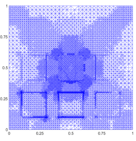
Figure 2. Test case I: spatial domain and subdomains (left) and the refined mesh after 18 iterations of Algorithm 5 using Leja collocation points (right).

The tolerance was satisfied after 32 spatial refinement steps and 6 parametric enrichment steps (38 iterations in total) for Leja points and after 30 spatial and 4 parametric enrichment steps (34 iterations in total) for CC points. The evolution of the error indicators and component error estimates is reported in Figure 3 and Figure 4, respectively. The key point here is that the combined error estimate $\eta_{\ell}:=\mu_{\ell}+\tau_{\ell}$ decreases at every iteration. In contrast, the total error indicator $\bar{\eta}_{\ell}:=\bar{\mu}_{\ell}+\bar{\tau}_{\ell}$ can be seen to increase at iterations that follow a parametric enrichment; see Figure 3. This is caused by a ‘jump’ of the spatial error indicator $\bar{\mu}_{\ell}$ that occurs every time when the set of collocation point expands. In addition to this, the mesh assigned to the new collocation point may be unsuitable for the sample of the diffusion coefficient at this point, which causes the growth of the two-level spatial error indicators associated with new collocation points in comparison with the spatial error indicators associated with previous collocation points. We have not observed ‘jumps’ for error estimates in the experiments we carried out; see, e.g., Figure 4. However, as we proved in Theorem 14, even if such ‘jumps’ occur, they are bounded by the terms converging to zero.

Figure 3. Test case I: evolution of the error indicators for Leja (left) and CC (right) points. The axes limits are identical in the left and right plots.

Figure 4. Test case I: evolution of the error estimates for Leja (left) and CC (right) points. The axes limits are identical in the left and right plots.

9.2. Test case II: nonaffine coefficient data

In this case, we set $f=1$ and solve the model problem (1) with coefficient $a(x,\mathbf{y})=\exp(h(x,\mathbf{y}))$ on the L-shaped domain $D=(-1,1)^{2}\backslash(-1,0]^{2}$. We set the exponent field $h(x,\mathbf{y})$ to have affine dependence on parameters $y_{m}$, i.e.,

$$h(x,\mathbf{y})=h_{0}(x)+\sum_{m=1}^{M}h_{m}(x)\,y_{m},\quad x\in D,\ \mathbf{y}\in\Gamma.$$ (56)

The expansion coefficients $h_{m}$, $m=0,1,\dots,M$, are chosen to represent planar Fourier modes of increasing total order. Thus, we fix $h_{0}(x):=1$ and set

$$h_{m}(x):=\alpha_{m}\cos(2\pi\beta_{1}(m)\,x_{1})\cos(2\pi\beta_{2}(m)\,x_{2}),\ x=(x_{1},x_{2})\in D.$$ (57)

The modes are ordered so that for any $m\in\mathbb{N}$,

$$\beta_{1}(m)=m-k(m)(k(m)+1)/2\ \ \hbox{and}\ \ \beta_{2}(m)=k(m)-\beta_{1}(m)$$ (58)

with $k(m)=\lfloor-1/2+\sqrt{1/4+2m}\rfloor$. Furthermore, to ensure that the diffusion coefficient satisfies (14), the amplitudes $\alpha_{m}$ in (57) are chosen as follows:

$$\alpha_{1}=0.498\ \ \text{and}\ \ \alpha_{m}=\bar{\alpha}m^{-1}\ \text{for $m=2,\dots,M$ with $\bar{\alpha}=0.547$}.$$ (59)

Indeed, differentiating the diffusion coefficient with respect to parameters, we obtain

$$\frac{\partial^{\mathbf{k}}a(\cdot,\mathbf{y})}{\partial\mathbf{y}^{\mathbf{k}}}=a(\cdot,\mathbf{y})\prod_{m=1}^{M}h^{k_{m}}_{m}(x).$$

Thus,

$$\left\lVert a^{-1}(\cdot,\mathbf{y})\,\frac{\partial^{\mathbf{k}}a(\cdot,\mathbf{y})}{\partial\mathbf{y}^{\mathbf{k}}}\right\rVert_{L^{\infty}(D)}=\left\lVert\ \prod_{m=1}^{M}h^{k_{m}}_{m}(x)\right\rVert_{L^{\infty}(D)}\leq\prod_{m=1}^{M}\alpha^{k_{m}}_{m}\leq(\mathbf{M}+\boldsymbol{1})^{-\mathbf{k}}\,\boldsymbol{\delta}^{-\mathbf{k}}\,\mathbf{k}!$$

for $\alpha_{m}$ given in (59) and for some vector $\boldsymbol{\delta}>\boldsymbol{1}$, as required by (14).

Figure 5. Test case II: evolution of the error indicators for Leja (left) and CC (right) points. The axes limits are identical in the left and right plots.

Figure 6. Test case II: evolution of the error estimates for Leja (left) and CC (right) points. The axes limits are identical in the left and right plots.

For this test case, we set the dimension of the parameter domain to $M=4$ and run Algorithm 5 with $\tt{errortolerance}=$ 2e-3. This tolerance was reached after 31 iterations (including 5 parametric refinement steps) for Leja points and after 31 iterations (including 3 parametric enrichments) for CC points. We record the evolution of spatial, parametric and cumulative error indicators as well as the evolution of the corresponding error estimates; see Figures 5 and 6. From these plots we can see that both the error indicators and the error estimates show similar behavior to that observed in Test Case I. Additionally, for both test cases, we observe that the execution of the algorithm with Leja collocation points requires more parametric enrichments than that with CC points to reach the same tolerance. This is explained by the fact that every new multi-index generates more collocation points of the CC type than those of the Leja type. For instance, in 1D, each index $i\in\mathbb{N}$ generates one new Leja collocation point and $2^{i-1}$ new CC points.

References

- [AO00] M. Ainsworth and J. T. Oden. A posteriori error estimation in finite element analysis. Pure and Applied Mathematics (New York). Wiley, 2000.
- [BCM17] M. Bachmayr, A. Cohen, and G. Migliorati. Sparse polynomial approximation of parametric elliptic PDEs. Part I: Affine coefficients. ESAIM Math. Model. Numer. Anal., 51(1):321–339, 2017.
- [Bie11] M. Bieri. A sparse composite collocation finite element method for elliptic SPDEs. SIAM J. Numer. Anal., 49(6):2277–2301, 2011.
- [BNT07] I. Babuška, F. Nobile, and R. Tempone. A stochastic collocation method for elliptic partial differential equations with random input data. SIAM J. Numer. Anal., 45(3):1005–1034, 2007.
- [BNTT11] J. Bäck, F. Nobile, L. Tamellini, and R. Tempone. Stochastic spectral Galerkin and collocation methods for PDEs with random coefficients: a numerical comparison. In Spectral and high order methods for partial differential equations, volume 76 of Lect. Notes Comput. Sci. Eng., pages 43–62. Springer, Heidelberg, 2011.
- [BPRR19a] A. Bespalov, D. Praetorius, L. Rocchi, and M. Ruggeri. Convergence of Adaptive Stochastic Galerkin FEM. SIAM J. Numer. Anal., 57(5):2359–2382, 2019.
- [BPRR19b] A. Bespalov, D. Praetorius, L. Rocchi, and M. Ruggeri. Goal-oriented error estimation and adaptivity for elliptic PDEs with parametric or uncertain inputs. Comput. Methods Appl. Mech. Engrg., 345:951–982, 2019.
- [BPS14] A. Bespalov, C. E. Powell, and D. Silvester. Energy norm a posteriori error estimation for parametric operator equations. SIAM J. Sci. Comput., 36(2):A339–A363, 2014.
- [BS16] A. Bespalov and D. Silvester. Efficient adaptive stochastic Galerkin methods for parametric operator equations. SIAM J. Sci. Comput., 38(4):A2118–A2140, 2016.
- [BS23] A. Bespalov and D. Silvester. Error estimation and adaptivity for stochastic collocation finite elements Part II: Multilevel approximation. SIAM J. Sci. Comput., 45(2):A784–A800, 2023.
- [BSX22] A. Bespalov, D. J. Silvester, and F. Xu. Error estimation and adaptivity for stochastic collocation finite elements Part I: Single-level approximation. SIAM J. Sci. Comput., 44(5):A3393–A3412, 2022.
- [BTNT12] J. Beck, R. Tempone, F. Nobile, and L. Tamellini. On the optimal polynomial approximation of stochastic PDEs by Galerkin and collocation methods. Math. Models Methods Appl. Sci., 22(9):1250023, 33, 2012.
- [BX20] A. Bespalov and F. Xu. A posteriori error estimation and adaptivity in stochastic Galerkin FEM for parametric elliptic PDEs: beyond the affine case. Comput. Math. Appl., 80(5):1084–1103, 2020.
- [CCS14] A. Chkifa, A. Cohen, and C. Schwab. High-dimensional adaptive sparse polynomial interpolation and applications to parametric PDEs. Found. Comput. Math., 14:601–633, 2014.
- [Chk13] M. A. Chkifa. On the Lebesgue constant of Leja sequences for the complex unit disk and of their real projection. J. Approx. Theory, 166:176–200, 2013.
- [EEST22] M. Eigel, O. G. Ernst, B. Sprungk, and L. Tamellini. On the convergence of adaptive stochastic collocation for elliptic partial differential equations with affine diffusion. SIAM Journal on Numerical Analysis, 60(2):659–687, 2022.
- [EST18] O. G. Ernst, B. Sprungk, and L. Tamellini. Convergence of sparse collocation for functions of countably many Gaussian random variables (with application to elliptic PDEs). SIAM J. Numer. Anal., 56(2):877–905, 2018.
- [FS21] M. Feischl and A. Scaglioni. Convergence of adaptive stochastic collocation with finite elements. Comput. Math. Appl., 98:139–156, 2021.
- [GG03] T. Gerstner and M. Griebel. Dimension-adaptive tensor-product quadrature. Computing, 71:65–87, 2003.
- [GN18] D. Guignard and F. Nobile. A posteriori error estimation for the stochastic collocation finite element method. SIAM J. Numer. Anal., 56(5):3121–3143, 2018.
- [KPP13] M. Karkulik, D. Pavlicek, and D. Praetorius. On 2D newest vertex bisection: Optimality of mesh-closure and -stability of -projection. Constr. Approx., 38:213–234, 2013.
- [LSS20] J. Lang, R. Scheichl, and D. Silvester. A fully adaptive multilevel stochastic collocation strategy for solving elliptic PDEs with random data. J. Comput. Phys., 419:109692, 17, 2020.
- [MSV08] P. Morin, K. G. Siebert, and A. Veeser. A basic convergence result for conforming adaptive finite elements. Math. Models Methods Appl. Sci., 18(5):707–737, 2008.
- [NTT16] F. Nobile, L. Tamellini, and R. Tempone. Convergence of quasi-optimal sparse-grid approximation of Hilbert-space-valued functions: application to random elliptic PDEs. Numer. Math., 134:343–388, 2016.
- [NTTT16] F. Nobile, L. Tamellini, F. Tesei, and R. Tempone. An adaptive sparse grid algorithm for elliptic PDEs with lognormal diffusion coefficient. In J. Garcke and D. Pflüger, editors, Sparse Grids and Applications—Stuttgart 2014, pages 191–220. Springer, 2016.
- [NTW08a] F. Nobile, R. Tempone, and C. G. Webster. An anisotropic sparse grid stochastic collocation method for partial differential equations with random input data. SIAM J. Numer. Anal., 46(5):2411–2442, 2008.
- [NTW08b] F. Nobile, R. Tempone, and C. G. Webster. A sparse grid stochastic collocation method for partial differential equations with random input data. SIAM J. Numer. Anal., 46(5):2309–2345, 2008.
- [Ste08] R. Stevenson. The completion of locally refined simplicial partitions created by bisection. Math. Comp., 77(261):227–241, 2008.