Convergence of the Adapted Smoothed Empirical Measures

Abstract

The adapted Wasserstein distance controls the calibration errors of optimal values in various stochastic optimization problems, pricing and hedging problems, optimal stopping problems, etc. Motivated by approximating the true underlying distribution by empirical data, we consider empirical measures of $\mathbb{R}^{d}$-valued stochastic process in finite discrete-time. It is known that the empirical measures do not converge under the adapted Wasserstein distance. To address this issue, we consider convolutions of Gaussian kernels and empirical measures as an alternative, which we refer to the Gaussian-smoothed empirical measures. By setting the bandwidths of Gaussian kernels depending on the number of samples, we prove the convergence of the Gaussian-smoothed empirical measures to the true underlying measure in terms of mean, deviation, and almost sure convergence. Although Gaussian-smoothed empirical measures converge to the true underlying measure and can potentially enlarge data, they are not discrete measures and therefore not applicable in practice. Therefore, we combine Gaussian-smoothed empirical measures and the adapted empirical measures in [AH22] to introduce the adapted smoothed empirical measures, which are discrete substitutes of the smoothed empirical measures. We establish the polynomial mean convergence rate, the exponential deviation convergence rate and the almost sure convergence of the adapted smoothed empirical measures.

Keywords: adapted Wasserstein distance, empirical measure, convergence rate
MSC (2020): 60B10, 62G30, 49Q22

1 Introduction

The development of the adapted Wasserstein distance is motivated by its robustness in stochastic optimization problems within a dynamic framework, as discussed in [PP14]. In stochastic finance, optimal values of various important problems, including pricing and hedging problems, optimal stopping problems, etc., are not continuous with respect to the Wasserstein distance. It’s worth noting that two stochastic models can be arbitrarily close to each other based on the Wasserstein distance, while their corresponding values in the aforementioned optimization problems can differ significantly. However, these optimal values are Lipschitz continuous with respect to the adapted Wasserstein distance, see [Bac+20, PP14]. This Lipschitz property implies that the adapted Wasserstein distance is strong enough to guarantee the robustness of path-dependent problems. On the other hand, the induced topology of adapted Wasserstein distance is not overstrong because it is the coarsest topology which makes optimal stopping values continuous. Therefore, the adapted Wasserstein distance is an appropriate metric when considering stochastic optimization problems under general probability distributions. For further details, please refer to [Bac+17, Las18, Rüs85, Bac+19, Pam22, ABP22, BW23].

Motivated by the Lipschitz property, we aim at building models that are close to the underlying measure under the adapted Wasserstein distance. However simply minimizing the adapted Wasserstein distance between models and empirical measures does not work, because empirical measures do not converge to the underlying measure under the adapted Wasserstein distance. To address this issue, Pflug-Pichler examine the smoothed empirical measures in [PP16] and establish their convergence in probability. As kernel-mixtures measures, smoothed empirical measures augment data and strengthen robustness in application, but they are not discrete, which restricts their applicability. Recently, Backhoff et al. introduce adapted empirical measures in [Bac+22] and establish their convergence. Surprisingly, adapted empirical measures recover the same optimal mean rate and deviation rate that are known for classical empirical measures with respect to the classical Wasserstein distance. Although adapted empirical measures are discrete, the projection of samples onto a grid leads to less distinct samples in practice. In summary, both measures have their own advantages and limitations in applications.

In this paper, we introduce the adapted smoothed empirical measures. We add Gaussian samples to our empirical samples and project the noised samples to grids as in the adapted empirical measures [Bac+22]. By this construction, adapted smoothed empirical measures are discrete measures. Moreover they allow one to augment data to any desired size meanwhile setting the grid size arbitrarily small. Despite the favorable practical properties mentioned above, we examine their convergence under the adapted Wasserstein distance. We prove that adapted smoothed empirical measures converge almost surely. Moreover, we prove almost optimal mean convergence rate and exponential deviation convergence rate. Our contributions in this paper are as follows:

• We establish the domination inequality between the weighted total variation and the adapted Wasserstein distance (Theorem 3.4).

• We generalize the convergence result of smoothed empirical measures under the adapted Wasserstein distance in [PP16] to the most general setting. We prove that Gaussian-smoothed empirical measures converge to $\mu$ almost surely (Theorem 2.15) as long as $\mu$ is integrable. Under additional assumptions, we prove polynomial mean convergence rate (Theorem 2.13) and exponential deviation convergence rate (Theorem 2.14).

• We establish the robustness of adapted Wasserstein distance with respect to Gaussian-noise perturbation. If $\mu$ is integrable, Gaussian-smoothed measures converge to $\mu$ almost surely (Theorem 2.10) as the variance of Gaussian noise goes to zero. If additionally $\mu$ has Lipschitz kernels, the convergence speed is linear (Theorem 2.12).

• We introduce the adapted smoothed empirical measures, which are discrete and allow data augmentation. We establish their convergence under adapted Wasserstein distance in mean, deviation and almost sure convergence (Theorem 2.23).

1.1 Related Literature

Smoothed empirical measure

Estimating the convergence of empirical measures under Wasserstein distance is a fundamental problem. Some seminal works are those by [GN21, Dud69, BGV07, BL14, DSS13, WB19, FG15, Lei18, BG10, Fou22]. Concerning empirical measures of stochastic processes, Pflug-Pichler [PP16] first noticed that empirical measures of stochastic processes do not converge to the true underlying measure under the adapted Wasserstein distance. To resolve this concern, they considered convolutions of smooth compact kernels with the empirical measures and analyzed their convergence when the underlying measures are compactly supported, with sufficiently regular densities bounded away from zero, and have uniformly Lipschitz kernels. If the kernels are non-negative and compactly supported, satisfying uniform consistency conditions, smoothed empirical measures converge in probability. Although their result does not hold for Gaussian kernels, the idea is essentially the same as that of Gaussian-smoothed empirical measures, and we are greatly inspired by their approach to introduce the adapted smoothed empirical measures in our work.

Adapted empirical measure

Backhoff et al. in [Bac+22] introduce the adapted empirical measures, which project paths onto a grid before taking the empirical measures, and establish almost sure convergence for measures with compact support. With further Lipschitz kernels assumption, they recover the same mean convergence rate as those for the Wasserstein distance in [FG15], which are sharp for all measures that are absolutely continuous with respect to the Lebesgue measure. Moreover, they prove the exponential concentration inequality under the same assumption. In [AH22], they have generalized these results beyond the compact assumption and proved convergence rates under finite moment and finite exponential moment conditions. In this paper, we crucially employ adapted empirical measures on $\mathbb{R}^{d}$ to prove convergence rate of the adapted smoothed empirical measures.

Organization of the paper. In Section 1, we give a brief introduction of the problem and elaborate our contributions. Then, in Section 2, we introduce the setting and state our main results. In Section 3, we introduce smooth distances and prove the convergence of empirical measures under various smooth distances. In Section 4, we analyze the bandwidth effect under adapted Wasserstein distance. In Section 5, we prove the convergence of smoothed empirical measures under adapted Wasserstein distance. In Section 6, we prove the convergence of adapted empirical smoothed measures under adapted Wasserstein distance. In Section 7, we prove the convergence of adapted smoothed empirical measures under adapted Wasserstein distance. Finally, in Appendix A, we collect some technical results and needed tools.

2 Setting and main results

Throughout the paper, we let $d\geq 3$ be the dimension of the state space and $T\geq 2$ be the time horizon. We consider finite discrete-time paths $x=x_{1:T}=(x_{1},\dots,x_{T})\in\mathbb{R}^{dT}$, where $x_{t}\in\mathbb{R}^{d}$ represents the value of the path at time $t=1,\dots,T$. We equip $\mathbb{R}^{dT}$ with a sum-norm $\|\cdot\|\colon\mathbb{R}^{dT}\to\mathbb{R}$ defined by $\|x\|=\sum_{t=1}^{T}\|x_{t}\|_{\mathbb{R}^{d}}$ for simplicity, but without loss of generality since all norms are equivalent on $\mathbb{R}^{dT}$. Let $\mathcal{P}(\mathbb{R}^{dT})$ be the space of canonical Borel probability measures on $\mathbb{R}^{dT}$, and let $\mu,\nu\in\mathcal{P}(\mathbb{R}^{dT})$. For $p\geq 1$, we denote by $M_{p}(\mu)=\int\|x\|^{p}\mu(dx)$ the $p$-th moment of $\mu$ and denote by $\mathcal{P}_{p}(\mathbb{R}^{dT})$ probability measures on $\mathbb{R}^{dT}$ with finite $p$-th moments. We let $(X^{(n)})_{n\in\mathbb{N}}$ be i.i.d. samples from $\mu$ defined on some probability space $(\Omega,\mathcal{F},{\mathbb{P}})$. For all $\sigma>0$, we denote by ${\mathcal{N}}_{\sigma}={\mathcal{N}}(\mathbf{0},\sigma^{2}\mathbf{I}_{dT})$ the Gaussian distribution and by $\varphi_{\sigma}$ its density function. Let $(\varepsilon^{(n,m)})_{n,m\in\mathbb{N}}$ be i.i.d. samples from ${\mathcal{N}}_{1}$ on $(\Omega,\mathcal{F},{\mathbb{P}})$ independent with $(X^{(n)})_{n\in\mathbb{N}}$. For all $\mu\in{\mathcal{P}}(\mathbb{R}^{dT})$, we call the convolution measure of $\mu$ and ${\mathcal{N}}_{\sigma}$ the Gaussian-smoothed measure of $\mu$ such that

$$(\mu\ast{\mathcal{N}}_{\sigma})(dx)=\int_{\mathbb{R}^{dT}}\varphi_{\sigma}(x-y)\mu(dy)dx,$$

and we denote $\mu\ast{\mathcal{N}}_{\sigma}$ by $\mu_{\sigma}$ for notational simplicity throughout the paper.

2.1 Adapted Wasserstein distance

In this section, we introduce different metrics on ${\mathcal{P}}(\mathbb{R}^{dT})$, in particular the adapted Wasserstein distance.

Definition 2.1 (Weighted total variation distance).

For $p\in[1,+\infty)$ and $\mu,\nu\in{\mathcal{P}}(\mathbb{R}^{dT})$, the $p$-th order weighed total variation distance $\mathrm{TV}_{p}(\cdot,\cdot)$ on $\mathcal{P}(\mathbb{R}^{dT})$ is defined by

$$\mathrm{TV}^{p}_{p}(\mu,\nu)=\int\big{\|}x\|^{p}|\mu-\nu|(dx),$$

where $|\mu-\nu|=\mu+\nu-2(\mu\wedge\nu)$.

Definition 2.2 (Wasserstein distance).

For $p\geq 1$ and $\mu,\nu\in{\mathcal{P}}(\mathbb{R}^{dT})$, the $p$-th order Wasserstein distance $\mathcal{W}_{p}(\cdot,\cdot)$ on $\mathcal{P}(\mathbb{R}^{dT})$ is defined by

$$\mathcal{W}_{p}^{p}(\mu,\nu)=\inf_{\pi\in\text{Cpl}(\mu,\nu)}\int\sum_{t=1}^{T}\big{\lVert}x_{t}-y_{t}\big{\rVert}^{p}_{\mathbb{R}^{d}}\pi(dx,dy),$$

where $\text{Cpl}(\mu,\nu)$ denotes the set of couplings between $\mu$ and $\nu$, that is, probabilities in $\mathcal{P}(\mathbb{R}^{dT}\times\mathbb{R}^{dT})$ with first marginal $\mu$ and second marginal $\nu$.

Next, we introduce the adapted Wasserstein distance. For notational simplicity, we denote by $x_{1:t}=(x_{1},...,x_{t})$, for $t=1,...,T$. For $\mu\in\mathcal{P}(\mathbb{R}^{dT})$, we denote the up to time $t$ marginal of $\mu$ by $\mu_{1:t}$, and the kernel (disintegration) of $\mu$ w.r.t. $x_{1:t}$ by $\mu_{x_{1:t}}$, so the following holds: $\mu(dx_{t+1})=\int_{\mathbb{R}^{dt}}\mu_{x_{1:t}}(dx_{t+1})\mu_{1:t}(dx_{1:t})$. Similarly, we denote the up to time $t$ marginal of $\pi\in\text{Cpl}(\mu,\nu)$ by $\pi_{1:t}$, and the kernel of $\pi$ w.r.t. $(x_{1:t},y_{1:t})$ by $\pi_{x_{1:t},y_{1:t}}$, so that $\pi(dx_{t+1},dy_{t+1})=\int_{\mathbb{R}^{dt}\times\mathbb{R}^{dt}}\pi_{x_{1:t},y_{1:t}}(dx_{t+1},dy_{t+1})\pi_{1:t}(dx_{1:t},dy_{1:t})$. For simplicity, we denote by $\pi_{1}=\pi_{1:1}=\pi_{x_{1:0},y_{1,0}}$. Now, we restrict our attention to couplings $\pi\in\text{Cpl}(\mu,\nu)$ such that the conditional law of $\pi$ is still a coupling of the conditional laws of $\mu$ and $\nu$, that is,

$$\pi_{x_{1:t},y_{1:t}}\in\text{Cpl}\big{(}\mu_{x_{1:t}},\nu_{y_{1:t}}\big{)}.$$ (1)

Such couplings are called bi-causal [Las18], and denoted by $\text{Cpl}_{\text{bc}}(\mu,\nu)$. The causality constraint can be expressed in different equivalent ways, see e.g. [Bac+17, ABZ20] in the context of transport, and [BY78] in the filtration enlargement framework. Roughly, in a causal transport, for every time $t$, only information on the $x$-coordinate up to time $t$ is used to determine the mass transported to the $y$-coordinate at time $t$. And in a bi-causal transport this holds in both directions, i.e. also when exchanging the role of $x$ and $y$.

As already mentioned in the Introduction, the adaptdness or bi-causality constraint turns out to be the correct one to impose on couplings, in order to modify the Wasserstein distance so to ensure robustness of stochastic optimization problems. That is to say, if two measures $\mu,\nu$ are close w.r.t. this distance, then solving w.r.t. $\mu$ optimization problems such as optimal stopping, optimal hedging, utility maximization etc, provides an “almost optimizer” for $\nu$; see [Bac+20].

Definition 2.3 (Adapted Wasserstein distance / Nested distance).

For $p\geq 1$ and $\mu,\nu\in{\mathcal{P}}(\mathbb{R}^{dT})$, the $p$-th order adapted Wasserstein distance $\mathcal{AW}_{p}$ on $\mathcal{P}(\mathbb{R}^{dT})$ is defined by

$$\mathcal{AW}^{p}_{p}(\mu,\nu)=\inf_{\pi\in\text{Cpl}_{\text{bc}}(\mu,\nu)}\int\sum_{t=1}^{T}\big{\lVert}x_{t}-y_{t}\big{\rVert}_{\mathbb{R}^{d}}^{p}\pi(dx,dy).$$ (2)

Bi-causal couplings and the corresponding optimal transport problem were considered by Rüschendorf [Rüs85] in so-called ‘Markov-constructions’. This concept was independently introduced by Pflug-Pichler [PP12] in the context of stochastic multistage optimization problems, see also [PP14], and also considered by Bion-Nadal and Talay in [BT19] and Gigli in [Gig08]. Pflug-Pichler refer to the adapted Wasserstein distance as nested distance, with an alternative representation through dynamic programming principle by disintegrating (2) and replacing conditional laws with (1). For notational simplicity, we state it here only for the case $T=2$, where one obtains the representation

$$\mathcal{AW}_{1}(\mu,\nu)=\inf_{\pi\in\text{Cpl}(\mu_{1},\nu_{1})}\int\|x_{1}-y_{1}\|_{\mathbb{R}^{d}}+\mathcal{W}_{1}(\mu_{x_{1}},\nu_{y_{1}})\pi(dx_{1},dy_{1}).$$

This reflects clearly that $\mathcal{AW}$ considers not only marginal laws but also the difference between conditional laws.

Example 2.4.

Let $\mu,\nu\in\mathcal{P}([0,1]^{2})$ be given by $\mu=\frac{1}{2}\delta_{(0,1)}+\frac{1}{2}\delta_{(0,-1)}$ and $\nu=\frac{1}{2}\delta_{(\epsilon,1)}+\frac{1}{2}\delta_{(-\epsilon,-1)}$, with $\epsilon\in(0,1)$, visualized in Figure 1. Then $\mathcal{W}(\mu,\nu)=\epsilon$, while $\mathcal{AW}(\mu,\nu)=1+\epsilon$, since $\mathcal{W}(\mu_{x_{1}},\nu_{y_{1}})=1$ no matter how we couple the first coordinate.

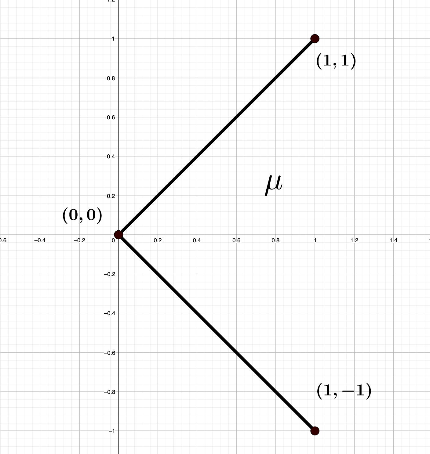
(a) $\mu=\frac{1}{2}\delta_{(0,1)}+\frac{1}{2}\delta_{(0,-1)}$

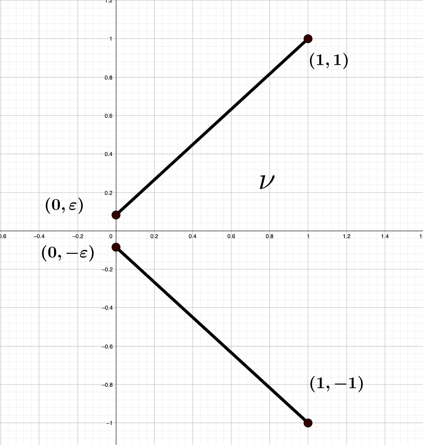
(b) $\nu=\frac{1}{2}\delta_{(\epsilon,1)}+\frac{1}{2}\delta_{(-\epsilon,-1)}$

Figure 1: Visualization of $\mu$ and $\nu$.

Let now consider a financial market with an asset whose law is described by $\mu$, and another market with an asset whose law is described by $\nu$. Then under the Wasserstein distance the two markets are judged as being close to each other, while they clearly present very different features (random versus deterministic evolution, no-arbitrage versus arbitrage, etc.). It is also evident how optimization problems in the two situations would lead to very different decision making. This is a standard example to motivate the introduction of adapted distances, that instead can distinguish between the two models.

2.2 Main results

In this section, we introduce the empirical measures and different variants of the empirical measures. Then we establish their convergence under the adapted Wasserstein distance.

Definition 2.5 (Empirical measures).

For all $N\in\mathbb{N}$, we denote by $\mu^{N}\coloneqq\frac{1}{N}\sum_{n=1}^{N}\delta_{X^{(n)}}$ the empirical measures of $\mu$, where $(X^{(n)})_{n\in\mathbb{N}}$ are i.i.d. samples from $\mu$.

2.2.1 Smoothed empirical measures with fixed bandwidth

First, we introduce the smoothed empirical measures by convoluting the empirical measures with Gaussian distribution.

Definition 2.6 (Smoothed empirical measures).

For all $N\in\mathbb{N}$ and $\sigma>0$, we call the convoluted measures of the empirical measures $\mu^{N}$ and ${\mathcal{N}}_{\sigma}$ the smoothed empirical measures of $\mu$, denoted by $\mu^{N}\ast{\mathcal{N}}_{\sigma}$.

With the bandwidth $\sigma$ fixed, the smoothed empirical measures $\mu^{N}\ast{\mathcal{N}}_{\sigma}$ converge to $\mu\ast{\mathcal{N}}_{\sigma}$ under adapted Wasserstein distance in terms of mean, deviation and almost sure convergence, see Section 3 for the proofs.

Theorem 2.7 (Mean convergence under smooth $\mathcal{AW}_{1}$).

Let $p>2$ and $\mu\in{\mathcal{P}}(\mathbb{R}^{dT})$ with finite $p$-th moment denoted by $M_{p}$. Then there exists $C_{\sigma,p,M_{p}}>0$ such that, for all $N\in\mathbb{N}$,

$$\mathbb{E}\left[\mathcal{AW}_{1}(\mu\ast{\mathcal{N}}_{\sigma},\mu^{N}\ast{\mathcal{N}}_{\sigma})\right]\leq C_{\sigma,p,M_{p}}N^{-\frac{1}{2}},$$

where $C_{\sigma,p,M_{p}}$ is given by (5) in Theorem 3.1.

Theorem 2.8 (Deviation convergence under smooth $\mathcal{AW}_{1}$).

Let $K\subseteq\mathbb{R}^{dT}$ be compact and $\mu\in{\mathcal{P}}(K)$. There exist $C_{\sigma,p,M_{p}},c_{\sigma,K}>0$ such that, for all $x>0$ and $N\in\mathbb{N}$

$${\mathbb{P}}\!\left(\mathcal{AW}_{1}(\mu\ast{\mathcal{N}}_{\sigma},\mu^{N}\ast{\mathcal{N}}_{\sigma})\geq x+C_{\sigma,p,M_{p}}N^{-\frac{1}{2}}\right)\leq e^{-\frac{Nx^{2}}{c_{\sigma,K}^{2}}},$$

where $C_{\sigma,p,M_{p}}$ is given by (5) in Theorem 3.1 and $c_{\sigma,K}$ is given by (9) in Theorem 3.3.

Theorem 2.9 (Almost sure convergence under smooth $\mathcal{AW}_{1}$).

Let $\mu\in{\mathcal{P}}(\mathbb{R}^{dT})$ integrable. Then

$$\lim_{N\to\infty}\mathcal{AW}_{1}(\mu\ast{\mathcal{N}}_{\sigma},\mu^{N}\ast{\mathcal{N}}_{\sigma})=0,\quad{\mathbb{P}}\text{-a.s.}$$

2.2.2 Bandwidth effect

It worths noticing that with the bandwidth $\sigma$ fixed, $\mu^{N}\ast{\mathcal{N}}_{\sigma}$ do converge to $\mu\ast{\mathcal{N}}_{\sigma}$ but not to the underlying measure $\mu$. In order to close the gap between $\mu\ast{\mathcal{N}}_{\sigma}$ and $\mu$, we now focus on the bandwidth effect of $\sigma$, namely the adapted Wasserstein distance between $\mu\ast\mathcal{N}_{\sigma}$ and $\mu$. We prove that as $\sigma$ approaches zero, $\mathcal{AW}_{1}(\mu,\mu\ast\mathcal{N}_{\sigma})$ converge to zero; see Section 4 for the proof.

Theorem 2.10 (Stability).

Let $\mu\in{\mathcal{P}}(\mathbb{R}^{dT})$ be integrable. Then

$$\lim_{\sigma\to 0}\mathcal{AW}_{1}(\mu,\mu\ast{\mathcal{N}}_{\sigma})=0.$$

Under additional assumption of Lipschitz kernels, the error can even be linearly controlled by $\sigma$; see Section 4 for the proof.

Definition 2.11.

Let $L>0$. We say that $\mu\in\mathcal{P}(\mathbb{R}^{dT})$ has $L$-Lipschitz kernels if there exists a disintegration s.t. for all $t=1,\dots,T-1$, $x_{1:t}\mapsto\mu_{x_{1:t}}$ is $L$-Lipschitz (${\mathcal{P}}(\mathbb{R}^{d})$ equipped with $\mathcal{W}_{1}$).

Theorem 2.12 (Lipschitz stability).

Let $L>0$ and $\mu\in{\mathcal{P}}(\mathbb{R}^{dT})$ with $L$-Lipschitz kernels. Then there exists $\tilde{C}_{L}>0$ s.t. for all $\sigma>0$,

$$\begin{split}\mathcal{AW}_{1}(\mu,\mu\ast{\mathcal{N}}_{\sigma})\leq\tilde{C}_{L}\sigma.\end{split}$$

2.2.3 Smoothed empirical measures with decaying bandwidth

The subsequent step is now evident that we combine the convergence with fixed bandwidth and the bandwidth effect. Setting $\sigma_{N}=N^{-r}$ and $\mathrm{rate}(N)={\mathcal{O}}(N^{-r})$ with $r=(dT+2)^{-1}$, we prove convergence of $\mu^{N}\ast{\mathcal{N}}_{\sigma_{N}}$ to $\mu$ under adapted Wasserstein distance, see Section 5 for the proofs.

Theorem 2.13 (Mean convergence under $\mathcal{AW}_{1}$).

Let $p>2$, $L>0$ and $\mu\in{\mathcal{P}}(\mathbb{R}^{dT})$ with finite $p$-th moment and $L$-Lipschitz kernels. Then there exists $C>0$ s.t. for all $N\in\mathbb{N}$,

$$\begin{split}\mathbb{E}\left[\mathcal{AW}_{1}(\mu,\mu^{N}\ast{\mathcal{N}}_{\sigma_{N}})\right]\leq CN^{-r}.\end{split}$$

Theorem 2.14 (Deviation convergence under $\mathcal{AW}_{1}$).

Let $K\subseteq\mathbb{R}^{dT}$ compact, $L>0$ and $\mu\in{\mathcal{P}}(K)$ with $L$-Lipschitz kernels. Then there exists $c_{K}>0$ such that for all $x>0$ and $N\in\mathbb{N}$,

$${\mathbb{P}}\Big{(}\mathcal{AW}_{1}(\mu,\mu^{N}\ast{\mathcal{N}}_{\sigma_{N}})\geq x+\mathrm{rate}(N)\Big{)}\leq e^{-\frac{x^{2}N^{1-r}}{c_{K}}}.$$

Theorem 2.15 (Almost sure convergence under $\mathcal{AW}_{1}$).

Let $\mu\in{\mathcal{P}}(\mathbb{R}^{dT})$ be integrable. Then

$$\lim_{N\to\infty}\mathcal{AW}_{1}(\mu,\mu^{N}\ast{\mathcal{N}}_{\sigma_{N}})=0,\quad{\mathbb{P}}\text{-a.s.}$$

Remark 2.16.

These theorems generalize the convergence result in [PP16] and further establish convergence rates in mean and deviation.

As we discussed above, the smoothed empirical measures converge but are still not discrete measures. Notice that the adapted empirical measures introduced in [Bac+22] converge and are discrete. Naturally, we combine the Gaussian-smoothing and adapted projection to construct the adapted smoothed empirical measures.

2.2.4 Adapted smoothed empirical measures

First, let us recall the definition of adapted empirical measures in [AH22].

Definition 2.17 (Adapted empirical measures).

For $N\in\mathbb{N}$ and grid size $\Delta_{N}>0$, we let ${\mathcal{M}}=\lceil\frac{1}{\Delta_{N}}\rceil$ and consider the uniform partition $\hat{\Phi}$ of $\mathbb{R}^{dT}$ given by

$$\hat{\Phi}^{N}=\left\{\hat{\mathcal{C}}_{\mathbf{z}}^{N}=\Big{[}0,\frac{1}{{\mathcal{M}}}\Big{]}^{dT}+\frac{1}{{\mathcal{M}}}\mathbf{z},\mathbf{z}\in\mathbb{Z}^{dT}\right\}.$$

Let $\hat{\Lambda}^{N}$ be the set of mid points of all cubes $\hat{\mathcal{C}}_{\mathbf{z}}^{N}$ in the partition $\hat{\Phi}^{N}$, and let $\hat{\varphi}^{N}\colon\mathbb{R}^{dT}\to\hat{\Lambda}^{N}$ map each cube $\hat{\mathcal{C}}_{\mathbf{z}}^{N}$ to its mid point (points belonging to more than one cube can be mapped into any of them). Then we denote by

$$\hat{\mu}^{N}=\frac{1}{N}\sum_{n=1}^{N}\delta_{\hat{\varphi}^{N}(X^{(n)})},$$

the adapted empirical measures of $\mu$ with grid size $\Delta_{N}$.

Remark 2.18.

Intuitively, the adapted empirical measure is constructed via the following procedure: (i) we tile $\mathbb{R}^{dT}$ with cubes of size $(\frac{1}{{\mathcal{M}}})^{dT}$ that form the partition $\hat{\Phi}^{N}$; (ii) we project all points in each cube $\hat{\mathcal{C}}_{\mathbf{z}}^{N}$ to its mid point. As a result, the push-forward measure obtained as empirical measures of the samples after projections is indeed the adapted empirical measure.

Next, we make a simple combination by considering the adapted empirical measures of Gaussian smoothed measure $\mu_{\sigma}=\mu\ast{\mathcal{N}}_{\sigma}$.

Definition 2.19 (Adapted empirical smoothed measures).

For all $N\in\mathbb{N}$ and $\sigma>0$, we call the adapted empirical measures of $\mu_{\sigma}$ the adapted empirical smoothed measures of $\mu$, denoted by $\hat{\mu}_{\sigma}^{N}$.

Setting $\sigma_{N}$ approaching zero, $\hat{\mu}_{\sigma_{N}}^{N}$ converge to $\mu$ under adapted Wasserstein distance, see Section 6. However, by Definition 2.19, the adapted empirical smoothed measures are still restricted to at most $N$ samples given $N$ i.i.d. samples of $\mu$ and therefore fail to augment dataset. Notice that an equivalent definition of $\hat{\mu}_{\sigma_{N}}^{N}$ is the following: $\hat{\mu}_{\sigma_{N}}^{N}=\frac{1}{N}\sum_{n=1}^{N}\delta_{\hat{\varphi}^{N}(X^{(n)}+\sigma_{N}\varepsilon^{(n,1)})}$, where $(\varepsilon^{(n,1)})_{n\in\mathbb{N}}$ are i.i.d. samples from ${\mathcal{N}}_{1}$. Inspired by this, we introduce the adapted smoothed empirical measures by copying each sample $X^{(n)}$ for $M$-many times and then adding independent Gaussian noise $(\varepsilon^{(n,m)})_{n,m\in\mathbb{N}}$ to each $X^{(n)}$, where $(\varepsilon^{(n,m)})_{n,m\in\mathbb{N}}$ are i.i.d. samples from ${\mathcal{N}}_{1}$.

Definition 2.20 (Adapted smoothed empirical measures).

For $N\in\mathbb{N}$ and grid size $\Delta_{N}>0$, we let ${\mathcal{M}}=\lceil\frac{1}{\Delta_{N}}\rceil$. For all $M\in\mathbb{N}$, we let $\zeta=(\zeta^{m})_{m=1}^{M}$ be $M$ distinct points in $(0,\frac{1}{2{\mathcal{M}}})^{dT}$ and denote by

$$\tilde{\mu}^{N,M}\vcentcolon=\frac{1}{M}\sum_{m=1}^{M}\tilde{\mu}^{N}_{\zeta,m},\quad\tilde{\mu}^{N}_{\zeta,m}=(x\mapsto x+\zeta^{m})\tilde{\mu}^{N}_{m},\quad\tilde{\mu}^{N}_{m}\vcentcolon=\frac{1}{N}\sum_{n=1}^{N}\delta_{\hat{\varphi}^{N}(X^{(n)}+\sigma_{N}\varepsilon^{(n,m)})},$$

the adapted smoothed empirical measures of $\mu$, where $\hat{\varphi}^{N}$ is the adapted projection in Definition 2.17, $\sigma_{N}=\Delta_{N}=N^{-r}$ with $r=(dT+2)^{-1}$. In particular, when $M=1$, we have $\tilde{\mu}^{N,1}=\hat{\mu}_{\sigma_{N}}^{N}$.

Table 1: Different measures

Symbol	Name	Convergence ($\mathcal{AW}_{1}$)	Discrete	Augment data
$\mu^{N}$	empirical measures	✗	✓	✗
$\mu_{\sigma_{N}}$	smoothed measures	✓  (Section 4)	✗	✗
$\mu^{N}\ast{\mathcal{N}}_{\sigma_{N}}$	smoothed empirical measures	✓  (Section 5)	✗	✓
$\hat{\mu}^{N}$	adapted empirical measures	✓  ([AH22])	✓	✗
$\hat{\mu}_{\sigma_{N}}^{N}$	adapted empirical smoothed measures	✓  (Section 6)	✓	✗
$\tilde{\mu}^{N,M}$	adapted smoothed empirical measures	✓  (Section 7)	✓	✓

Remark 2.21.

The adapted projection is necessary; without it, adapted smoothed empirical measures fail to converge. By taking $\mu$ a Dirac measure, it boils down to that empirical measures of Gaussian distribution do not converge to the underlying measure under the adapted Wasserstein distance.

Remark 2.22.

The introduction of $(\zeta^{m})_{m=1}^{M}$ is technical. Without $(\zeta^{m})_{m=1}^{M}$, all $(\tilde{\mu}^{M}_{m})_{m=1}^{M}$ are supported on the same grid $\hat{\Lambda}^{N}$. Then some measures might have intersection on the support. Since the adapted Wasserstein distance is so sensitive to the support that it is not convex w.r.t. its marginal, see Example A.3 for a counterexample. However with $(\zeta^{m})_{m=1}^{M}$ distinct introduced, $(\hat{\Lambda}^{N}+\zeta^{m})_{m=1}^{M}$ are distinct grids such that $(\tilde{\mu}^{M}_{\zeta,m})_{m=1}^{M}$ has no intersection in the support. This allows us to decouple bicausal couplings on distinct supports to establish convexity of the adapted Wasserstein distance, see Lemma A.2 for details. Also we choose $(\zeta^{m})_{m=1}^{M}$ from $(0,\frac{1}{2{\mathcal{M}}})^{dT}$ such that the shifting error is absorbed by ${\mathcal{O}}(N^{-r})$.

The adapted smoothed empirical measures are discrete and able to augment dataset by increasing $M$. Next, we show their convergence under the adapted Wasserstein distance and establish the convergence rates in mean, deviation and almost sure convergence; see Section 7 for the proof.

Theorem 2.23.

Let $L>0$, $\alpha\geq 2$, $\gamma>0$, $\mu\in\mathcal{P}(\mathbb{R}^{dT})$ with finite $(\alpha,\gamma)$-exponential moment. Assume that $\sup_{x_{1:t}\in\mathbb{R}^{dt}}{\mathcal{E}}_{\alpha,2^{\alpha}\gamma}(\mu_{x_{1:t}})<\infty$ for all $t=1,\dots,T-1$ and that for all $\sigma\in(0,1]$, $\mu\ast{\mathcal{N}}_{\sigma}$ has $L$-Lipschitz kernels. Then there exist constants $c,C>0$ s.t. for all $x>0$ and $N,M\in\mathbb{N}$,

$$\mathbb{E}\big{[}\mathcal{AW}_{1}(\mu,\tilde{\mu}^{N,M})\big{]}\leq CN^{-r},$$

and

$${\mathbb{P}}\Big{(}\mathcal{AW}_{1}(\mu,\tilde{\mu}^{N,M})\geq x+\mathrm{rate}(N)\Big{)}\leq CMe^{-cNx^{2}},$$

where $\mathrm{rate}(N)={\mathcal{O}}(N^{-r})$, $r=(dT+2)^{-1}$. Moreover,

$$\lim_{N\to\infty}\mathcal{AW}_{1}(\mu,\tilde{\mu}^{N,M})=0,\quad{\mathbb{P}}\text{-a.s.}$$ (3)

We conclude this section by illustrating a widely recognized probabilistic model that exemplifies the fulfillment of the assumption of Theorem 2.23.

Example 2.24 (Gaussian mixture model).

Let $K\in\mathbb{N}$ and $\mu\in{\mathcal{P}}(\mathbb{R}^{dT})$ with density $p_{\mu}(x)=\sum_{k=1}^{K}w_{k}\varphi_{\sigma^{k}}(x-x^{k})$, where $\sum_{k=1}^{K}w_{k}=1$, $w_{k}\geq 0,\sigma^{k}\geq 0$, $x^{k}\in\mathbb{R}^{dT}$ for all $k=1,\dots,K$. The assumption of Theorem 2.23 is satisfied, see Appendix A.2 for details.

3 Smooth distances

Throughout this section, we fix the bandwidth $\sigma$ and analyze the error between Gaussian-smoothed empirical measures $\mu^{N}\ast{\mathcal{N}}_{\sigma}$ and the Gaussian-smoothed underlying measure $\mu_{\sigma}=\mu\ast{\mathcal{N}}_{\sigma}$. For simplicity, we refer to the distance between two smoothed measures as the smooth distance between the measures.

3.1 Convergence under smooth $\mathrm{TV}_{1}$

We begin by establishing convergence results under the weighted total variation distance, and then generalize results to the adapted Wasserstein distance.

Theorem 3.1 (Mean convergence under smooth $\mathrm{TV}_{1}$).

Let $p>2$ and $\mu\in{\mathcal{P}}(\mathbb{R}^{dT})$ with finite $p$-th moment denoted by $M_{p}$. Then there exist $C_{1},C_{2}>0$ such that, for all $N\in\mathbb{N}$,

$$\mathbb{E}\Big{[}\mathrm{TV}_{1}(\mu\ast{\mathcal{N}}_{\sigma},\mu^{N}\ast{\mathcal{N}}_{\sigma})\Big{]}\leq C_{\sigma,p,M_{p}}N^{-\frac{1}{2}},$$ (4)

where

$$C_{\sigma,p,M_{p}}=\left(\int\frac{\|x\|^{2}}{1+\|x\|^{p}}dx\right)^{\frac{1}{2}}\sqrt{\big{(}C_{1}(2^{p}M_{p}+1)+C_{2}2^{p}\sigma^{p}\big{)}\frac{1}{(2\pi\sigma)^{dT}}}.$$ (5)

Proof.

The proof is similar to the proof of Proposition 2 in [Gol+20] and w.l.o.g. we use the 2-norm $\|x\|=\left(\sum_{t=1}^{T}\lVert x_{t}-y_{t}\rVert_{2}^{2}\right)^{\frac{1}{2}}$ for simplicity. Recall that we denote the density of the Gaussian kernel by $\varphi_{\sigma}$. Since $\varphi_{\sigma}$ is smooth, by convolution, $\mu\ast{\mathcal{N}}_{\sigma}$ and $\mu^{N}\ast{\mathcal{N}}_{\sigma}$ also have smooth densities, and we denote them by $q$ and $q^{N}$. Let $f_{p}\colon\mathbb{R}^{dT}\to\mathbb{R}_{\geq 0}$ s.t. $f_{p}(x)=\frac{1}{1+\|x\|^{p}}$ for all $x\in\mathbb{R}^{dT}$. By Cauchy-Schwarz, we have

$$\begin{split}\mathbb{E}\Big{[}\mathrm{TV}_{1}(\mu\ast{\mathcal{N}}_{\sigma},\mu^{N}\ast{\mathcal{N}}_{\sigma})\Big{]}&=\mathbb{E}\Big{[}\int\|x\||q-q_{N}|(x)dx\Big{]}\\ &\leq\left(\int\|x\|^{2}f_{p}(x)dx\right)^{\frac{1}{2}}\left(\int\frac{\mathbb{E}\left[(q(x)-q_{N}(x))^{2}\right]}{f_{p}(x)}dx\right)^{\frac{1}{2}}.\end{split}$$ (6)

Notice that $\mathbb{E}[q_{N}(x)]=q(x)$. We have

$$\begin{split}\mathbb{E}\Big{[}(q(x)-q_{N}(x))^{2}\Big{]}&=\mathrm{Var}\left[q_{N}(x)\right]=\mathrm{Var}\Big{[}\frac{1}{N}\sum_{i=1}^{N}\varphi_{\sigma}(x-X^{(i)})\Big{]}=\frac{1}{N}\mathrm{Var}\Big{[}\varphi_{\sigma}(x-X^{(1)})\Big{]}\\ &\leq\frac{1}{N}\mathbb{E}\Big{[}\varphi^{2}_{\sigma}(x-X^{(1)})\Big{]}=\frac{1}{N}\frac{1}{(2\pi\sigma^{2})^{dT}}\mathbb{E}\Big{[}e^{-\frac{\|x-X^{(1)}\|^{2}}{\sigma^{2}}}\Big{]}.\end{split}$$

This implies that

$$\int\frac{\mathbb{E}\Big{[}(q(x)-q_{N}(x))^{2}\Big{]}}{f_{p}(x)}dx\leq\frac{1}{(2\pi\sigma^{2})^{dT}}\cdot\frac{1}{N}\mathbb{E}\Big{[}\int\frac{1}{f_{p}(x)}\cdot e^{-\frac{\|x-X^{(1)}\|^{2}}{\sigma^{2}}}dx\Big{]}.$$ (7)

Notice that

$$\begin{split}&\quad\mathbb{E}\Big{[}\int\frac{1}{f_{p}(x)}\cdot e^{-\frac{\|x-X\|^{2}}{\sigma^{2}}}dx\Big{]}=\int\int\frac{1}{f_{p}(x)}\cdot e^{-\frac{\|x-z\|^{2}}{\sigma^{2}}}dx\mu(dz)=\int\int\frac{1}{f_{p}(z+y)}\cdot e^{-\frac{\|y\|^{2}}{\sigma^{2}}}dy\mu(dz),\quad(x=y+z)\\ &=\int\int(\|z+y\|^{p}+1)\cdot e^{-\frac{\|y\|^{2}}{\sigma^{2}}}dy\mu(dz)\leq\int\int\left(2^{p}\left(\|z\|^{p}+\|y\|^{p}\right)+1\right)\cdot e^{-\frac{\|y\|^{2}}{\sigma^{2}}}dy\mu(dz)\\ &=\int(2^{p}\|z\|^{p}+1)\int e^{-\frac{\|y\|^{2}}{\sigma^{2}}}dy\mu(dz)+\int 2^{p}\|y\|^{p}\cdot e^{-\frac{\|y\|^{2}}{\sigma^{2}}}dy\\ &=\int(2^{p}\|z\|^{p}+1)\int\sigma^{dT}e^{-\|u\|^{2}}du\mu(dz)+\int 2^{p}\sigma^{dT+p}\|u\|^{p}\cdot e^{-\|u\|^{2}}du,\quad(y=\sigma u)\\ &=C_{1}\sigma^{dT}\int(2^{p}\|z\|^{p}+1)\mu(dz)+C_{2}2^{p}\sigma^{dT+p}=\sigma^{dT}\big{(}C_{1}(2^{p}M_{p}+1)+C_{2}2^{p}\sigma^{p}\big{)}.\end{split}$$

where $C_{1}$ and $C_{2}$ are appropriate constants. Therefore, by combining this, (6) and (7), we obtain that

$$\mathbb{E}\Big{[}\mathrm{TV}_{1}(\mu\ast{\mathcal{N}}_{\sigma},\mu^{N}\ast{\mathcal{N}}_{\sigma})\Big{]}\leq\left(\int\frac{\|x\|^{2}}{1+\|x\|^{p}}dx\right)^{\frac{1}{2}}\sqrt{\big{(}C_{1}(2^{p}M_{p}+1)+C_{2}2^{p}\sigma^{p}\big{)}\frac{1}{(2\pi\sigma)^{dT}}\frac{1}{N}}.$$

Therefore, by setting

$$C_{\sigma,p,M_{p}}=\left(\int\frac{\|x\|^{2}}{1+\|x\|^{p}}dx\right)^{\frac{1}{2}}\sqrt{\big{(}C_{1}(2^{p}M_{p}+1)+C_{2}2^{p}\sigma^{p}\big{)}\frac{1}{(2\pi\sigma)^{dT}}},$$

we prove (4). ∎

Remark 3.2.

Theorem 3.1 holds not only for Gaussian kernel ${\mathcal{N}}_{\sigma}$, but also for a broad class of sub-Gaussian kernels. Let ${\mathcal{G}}_{\sigma}\in{\mathcal{P}}(\mathbb{R}^{dT})$ with density $g_{\sigma}$ that decomposes as $g_{\sigma}(x)=\prod_{j=1}^{dT}\tilde{g}_{\sigma}(x_{j})$ and the measure with density $\tilde{g}_{\sigma}$ is $\sigma$-subgaussian, bounded and monotonically decreasing as its argument goes away from zero in either direction. Let $\delta=\min\{1,\frac{1}{4\sigma^{2}}\}$, then by Lemma 2 in [GG20], there exists a constant $c_{1}>0$ s.t.

$$g_{\sigma}(x)\leq c_{1}^{dT}e^{\delta\|x\|^{2}}\varphi_{\sigma}(x),\quad\forall x\in\mathbb{R}^{dT}.$$

Then by replacing ${\mathcal{N}}_{\sigma}$ with ${\mathcal{G}}_{\sigma}$, Theorem 3.1 still holds but with a different constant. For details, see [GG20].

Theorem 3.3 (Deviation convergence under smooth $\mathrm{TV}_{1}$).

Let $K\subseteq\mathbb{R}^{dT}$ be compact and $\mu\in{\mathcal{P}}(K)$. Then there exists $c_{1}>0$ s.t. for all $x>0$ and $N\in\mathbb{N}$,

$${\mathbb{P}}\Big{(}\mathrm{TV}_{1}(\mu\ast{\mathcal{N}}_{\sigma},\mu^{N}\ast{\mathcal{N}}_{\sigma})-\mathbb{E}\!\left[\mathrm{TV}_{1}(\mu\ast{\mathcal{N}}_{\sigma},\mu^{N}\ast{\mathcal{N}}_{\sigma})\right]\geq x\Big{)}\leq e^{-\frac{Nx^{2}}{c_{\sigma,K}^{2}}},$$ (8)

where

$$c_{\sigma,K}=c_{1}(\sup_{x\in K}\frac{\|x\|}{\sigma}+1).$$ (9)

Proof.

In the proof, we apply McDiarmid’s inequality, see [McD89], to $\mathrm{TV}_{1}(\mu\ast{\mathcal{N}}_{\sigma},\mu^{N}\ast{\mathcal{N}}_{\sigma})$. First, we derive a variational expression of $\mathrm{TV}_{1}(\mu\ast{\mathcal{N}}_{\sigma},\mu^{N}\ast{\mathcal{N}}_{\sigma})$. Let ${\mathcal{F}}=\{f\in{\mathcal{B}}(\mathbb{R}^{d},\mathbb{R})\colon f(x)\leq\|x\|,\forall x\in\mathbb{R}^{dT}\}$, ${\mathcal{F}}_{\sigma}=\{f\ast\varphi_{\sigma}\colon f\in{\mathcal{F}}\}$. Since $\varphi_{\sigma}$ is smooth, then by convolution, $\mu\ast{\mathcal{N}}_{\sigma}$ and $\mu^{N}\ast{\mathcal{N}}_{\sigma}$ also have smooth densities, and we denote them by $q$ and $q^{N}$. Let $f^{*}(x)=\mathrm{sign}(q^{N}(x)-q(x))\cdot\|x\|\in{\mathcal{F}}$. Then, we have

$$\begin{split}\mathrm{TV}_{1}(\mu\ast{\mathcal{N}}_{\sigma},\mu^{N}\ast{\mathcal{N}}_{\sigma})&=\int\|x\||q(x)-q^{N}(x)|dx=\int f^{*}(x)q^{N}(x)dx-\int f^{*}(x)q(x)dx\\ &=\sup_{f\in{\mathcal{F}}}\int_{\mathbb{R}^{dT}}f(x)\left(\int_{\mathbb{R}^{dT}}\varphi_{\sigma}(x-y)\mu^{N}(dy)-\int_{\mathbb{R}^{dT}}\varphi_{\sigma}(x-y)\mu(dy)\right)dx\\ &=\sup_{f\in{\mathcal{F}}}\int_{\mathbb{R}^{dT}}(f\ast\varphi_{\sigma})(y)\mu^{N}(dy)-\int_{\mathbb{R}^{dT}}(f\ast\varphi_{\sigma})(y)\mu(dy)\\ &=\sup_{f\in{\mathcal{F}}}\frac{1}{N}\sum_{n=1}^{N}(f\ast\varphi_{\sigma})(X^{(n)})-\int_{\mathbb{R}^{dT}}(f\ast\varphi_{\sigma})(y)\mu(dy).\end{split}$$ (10)

Let $F\colon K^{N}\to\mathbb{R}$ s.t. for all $(x_{1},\dots,x_{N})\in K^{N}$,

$$F(x_{1},\dots,x_{N})=\sup_{f\in{\mathcal{F}}}\frac{1}{N}\sum_{n=1}^{N}(f\ast\varphi_{\sigma})(x_{n})-\int_{\mathbb{R}^{dT}}(f\ast\varphi_{\sigma})(y)\mu(dy).$$

Next, we show that $F$ satisfies the conditions to apply the McDiarmid’s inequality. For all $(x_{1},\dots,x_{N})$, $(x_{1}^{\prime},\dots,x_{N}^{\prime})\in K^{N}$ that differ only in the $i$-th coordinate, $i=1,\dots,N$, we have that

$$\begin{split}&\quad F(x_{1},\dots,x_{N})-F(x^{\prime}_{1},\dots,x^{\prime}_{N})\\ &=\sup_{f\in{\mathcal{F}}}\left(\frac{1}{N}\sum_{n=1}^{N}(f\ast\varphi_{\sigma})(x_{n})-\int_{\mathbb{R}^{dT}}(f\ast\varphi_{\sigma})(y)\mu(dy)\right)-\sup_{g\in{\mathcal{F}}}\left(\frac{1}{N}\sum_{n=1}^{N}(g\ast\varphi_{\sigma})(x^{\prime}_{n})-\int_{\mathbb{R}^{dT}}(g\ast\varphi_{\sigma})(y)\mu(dy)\right)\\ &\leq\sup_{f\in{\mathcal{F}}}\frac{1}{N}\sum_{n=1}^{N}(f\ast\varphi_{\sigma})(x_{n})-\frac{1}{N}\sum_{n=1}^{N}(f\ast\varphi_{\sigma})(x^{\prime}_{n})=\sup_{f\in{\mathcal{F}}}\frac{1}{N}(f\ast\varphi_{\sigma})(x_{i})-\frac{1}{N}(f\ast\varphi_{\sigma})(x^{\prime}_{i}).\end{split}$$ (11)

Notice that for all $f\in{\mathcal{F}}$, $x=(x^{(1)},\dots,x^{(dT)})\in K$ and $j=1,\cdots,dT$,

$$\begin{split}\frac{\partial}{\partial x^{(j)}}(f\ast\varphi_{\sigma})(x)&=\frac{\partial}{\partial x^{(j)}}\int_{\mathbb{R}^{dT}}\varphi_{\sigma}(x-y)f(y)dy=\int_{\mathbb{R}^{dT}}\frac{\partial}{\partial x^{(j)}}\varphi_{\sigma}(x-y)f(y)dy\\ &=-\int_{\mathbb{R}^{dT}}\frac{y^{(j)}-x^{(j)}}{\sigma^{2}}\varphi_{\sigma}(y-x)f(y)dy=-\int_{\mathbb{R}^{dT}}\frac{z^{(j)}}{\sigma^{2}}\varphi_{\sigma}(z)f(x+z)dz,\quad(z=y-x)\\ &\leq\int_{\mathbb{R}^{dT}}\frac{|z^{(j)}|}{\sigma^{2}}\varphi_{\sigma}(z)\|x+z\|dz=\int_{\mathbb{R}^{dT}}|\frac{u^{(j)}}{\sigma}|\varphi_{1}(u)\|x+\sigma u\|du,\quad(z=\sigma u)\\ &\leq\int_{\mathbb{R}^{dT}}\frac{\|x\|}{\sigma}|u^{(j)}|\varphi_{1}(u)du+\int_{\mathbb{R}^{dT}}|u^{(j)}|\varphi_{1}(u)\|u\|du\\ &\leq(\frac{\|x\|}{\sigma}+1)\int_{\mathbb{R}^{dT}}|u^{(j)}|(1+\|u\|)\varphi_{1}(u)du\leq(\sup_{x\in K}\frac{\|x\|}{\sigma}+1)\int_{\mathbb{R}^{dT}}|u^{(j)}|(1+\|u\|)\varphi_{1}(u)du.\end{split}$$

Let $c_{1}=\int_{\mathbb{R}^{dT}}|u^{(1)}|(1+\|u\|)\varphi_{1}(u)du$ and $c_{\sigma,K}=c_{1}(\sup_{x\in K}\frac{\|x\|}{\sigma}+1)$. Thus for all $x,x^{\prime}\in K$, we have

$$\sup_{f\in{\mathcal{F}}}|(f\ast\varphi_{\sigma})(x)-(f\ast\varphi_{\sigma})(x^{\prime})|\leq c_{\sigma,K}\|x-x^{\prime}\|.$$

Combine this with (11). We have for all $(x_{1},\dots,x_{N})$, $(x_{1}^{\prime},\dots,x_{N}^{\prime})\in K^{N}$ that differ only in the $i$-th coordinate, $i=1,\dots,N$, $F(x_{1},\dots,x_{N})-F(x^{\prime}_{1},\dots,x^{\prime}_{N})\leq\frac{c_{\sigma,K}}{N}\|x_{i}-x^{\prime}_{i}\|$. Therefore, we can apply McDiarmid’s inequality, see [McD89], to conclude that for all $x>0$, $N\in\mathbb{N}$,

$${\mathbb{P}}\Big{(}F(X^{(1)},\dots,X^{(N)})-\mathbb{E}[F(X^{(1)},\dots,X^{(N)})]\geq x\Big{)}\leq e^{-\frac{Nx^{2}}{c_{\sigma,K}^{2}}}.$$

Combining this, the definition of $F$ and (10), we prove (8). ∎

3.2 Convergence under smooth $\mathcal{AW}_{1}$

First, we show that the weighted total variation is stronger than the adapted Wasserstein distance.

Theorem 3.4 (Metric dominations).

Let $\mu,\nu\in{\mathcal{P}}(\mathbb{R}^{dT})$ be such that the distances below are well-defined. Then

$$\mathcal{W}_{1}(\mu,\nu)\leq\mathcal{AW}_{1}(\mu,\nu)\leq\mathrm{TV}_{1}(\mu,\nu).$$

Proof.

It is obvious that $\mathcal{W}_{1}\leq\mathcal{AW}_{1}$, because any bi-causal coupling is a coupling. Thus, we remain to prove that $\mathcal{AW}_{1}\leq\mathrm{TV}_{1}$. For notational simplicity, we denote the marginals at time $t=1$ by $\mu_{x_{1:0}}=\mu_{1}$ and $\nu_{y_{1:0}}=\nu_{1}$. The idea of the proof is to construct a bi-causal coupling $\pi^{\mathrm{bc}}\in\text{Cpl}_{\text{bc}}(\mu,\nu)$ such that $\int\|x-y\|\pi^{\mathrm{bc}}(dx,dy)$ is dominated by $\mathrm{TV}_{1}(\mu,\nu)$. The main ingredient to construct such $\pi^{\mathrm{bc}}$ is the total variation coupling. For all $t=0,\dots,T-1$ and $x_{1:t},y_{1:t}\in\mathbb{R}^{dt}$, we define the total variation coupling $\gamma^{\mathrm{tv}}_{x_{1:t},y_{1:t}}\in\text{Cpl}(\mu_{x_{1:t}},\nu_{y_{1:t}})$ by

$$\left\{\begin{aligned} \gamma^{\mathrm{tv}}_{x_{1:t},y_{1:t}}&=\gamma^{\mathrm{id}}_{x_{1:t},y_{1:t}}+\gamma^{\mathrm{sd}}_{x_{1:t},y_{1:t}},\\ \gamma^{\mathrm{id}}_{x_{1:t},y_{1:t}}&=(\mathbf{id},\mathbf{id})_{\#}(\mu_{x_{1:t}}\wedge\nu_{y_{1:t}}),\\ \gamma^{\mathrm{sd}}_{x_{1:t},y_{1:t}}&=(\mu_{x_{1:t}}-\mu_{x_{1:t}}\wedge\nu_{y_{1:t}})\otimes(\nu_{y_{1:t}}-\mu_{x_{1:t}}\wedge\nu_{y_{1:t}}).\end{aligned}\right.$$

Now we can construct $\pi^{\mathrm{bc}}$ iteratively by kernels s.t.

$$\pi^{\mathrm{bc}}(dx_{1:T},dy_{1:T})=\pi^{\mathrm{bc}}_{1}(dx_{1},dy_{1})\prod_{t=1}^{T-1}\pi^{\mathrm{bc}}_{x_{1:t},y_{1:t}}(dx_{t+1},dy_{t+1}),$$

where the first marginal distribution $\pi^{\mathrm{bc}}_{1}$ and kernels $\pi^{\mathrm{bc}}_{x_{1:t},y_{1:t}}$ are defined by

$$\left\{\begin{aligned} \pi^{\mathrm{bc}}_{1}&=\gamma^{\mathrm{tv}}_{x_{1:0},y_{1:0}},\\ \pi^{\mathrm{bc}}_{x_{1:t},y_{1:t}}&=\delta_{\{x_{1:t}=y_{1:t}\}}\gamma^{\mathrm{tv}}_{x_{1:t},y_{1:t}}+\delta_{\{x_{1:t}\neq y_{1:t}\}}\left(\mu_{x_{1:t}}\otimes\nu_{y_{1:t}}\right),\quad\forall t=1,\dots,T-1.\end{aligned}\right.$$

Note that $\gamma^{\mathrm{tv}}_{x_{1:t},y_{1:t}}\in\text{Cpl}(\mu_{x_{1:t}},\nu_{y_{1:t}})$ and $\left(\mu_{x_{1:t}}\otimes\nu_{y_{1:t}}\right)\in\text{Cpl}(\mu_{x_{1:t}},\nu_{y_{1:t}})$. Thus, we have $\pi^{\mathrm{bc}}_{x_{1:t},y_{1:t}}\in\text{Cpl}(\mu_{x_{1:t}},\nu_{y_{1:t}})$, which implies that $\pi^{\mathrm{bc}}\in\text{Cpl}_{\text{bc}}(\mu,\nu)$ by definition. Next, we prove that $\pi^{\mathrm{bc}}$ satisfies that $\int\|x-y\|\pi^{\mathrm{bc}}(dx,dy)\leq\mathrm{TV}_{1}(\mu,\nu)$. Notice that

$$\begin{split}\pi^{\mathrm{bc}}&=\pi^{\mathrm{bc}}_{1}\prod_{t=1}^{T-1}\pi^{\mathrm{bc}}_{x_{1:t},y_{1:t}}=\Big{(}\gamma^{\mathrm{id}}_{x_{1:0},y_{1:0}}+\gamma^{\mathrm{sd}}_{x_{1:0},y_{1:0}}\Big{)}\Big{(}\delta_{\{x_{1}=y_{1}\}}\gamma^{\mathrm{tv}}_{x_{1},y_{1}}+\delta_{\{x_{1}\neq y_{1}\}}\left(\mu_{x_{1}}\otimes\nu_{y_{1}}\right)\Big{)}\prod_{t=2}^{T-1}\pi^{\mathrm{bc}}_{x_{1:t},y_{1:t}}\\ &=\Big{(}\gamma^{\mathrm{id}}_{x_{1:0},y_{1:0}}+\gamma^{\mathrm{sd}}_{x_{1:0},y_{1:0}}\Big{)}\Big{(}\delta_{\{x_{1}=y_{1}\}}\gamma^{\mathrm{id}}_{x_{1},y_{1}}+\delta_{\{x_{1}=y_{1}\}}\gamma^{\mathrm{sd}}_{x_{1},y_{1}}+\delta_{\{x_{1}\neq y_{1}\}}\left(\mu_{x_{1}}\otimes\nu_{y_{1}}\right)\Big{)}\prod_{t=2}^{T-1}\pi^{\mathrm{bc}}_{x_{1:t},y_{1:t}}\\ &=\Big{(}\gamma^{\mathrm{id}}_{x_{1:0},y_{1:0}}\gamma^{\mathrm{id}}_{x_{1},y_{1}}+\gamma^{\mathrm{id}}_{x_{1:0},y_{1:0}}\gamma^{\mathrm{sd}}_{x_{1},y_{1}}+\gamma^{\mathrm{sd}}_{x_{1:0},y_{1:0}}\left(\mu_{x_{1}}\otimes\nu_{y_{1}}\right)\Big{)}\prod_{t=2}^{T-1}\pi^{\mathrm{bc}}_{x_{1:t},y_{1:t}}\\ &=\Big{(}\gamma^{\mathrm{id}}_{x_{1:0},y_{1:0}}\gamma^{\mathrm{id}}_{x_{1},y_{1}}\gamma^{\mathrm{id}}_{x_{1:2},y_{1:2}}+\gamma^{\mathrm{id}}_{x_{1:0},y_{1:0}}\gamma^{\mathrm{id}}_{x_{1},y_{1}}\gamma^{\mathrm{sd}}_{x_{1:2},y_{1:2}}+\gamma^{\mathrm{id}}_{x_{1:0},y_{1:0}}\gamma^{\mathrm{sd}}_{x_{1},y_{1}}\left(\mu_{x_{1:2}}\otimes\nu_{y_{1:2}}\right)\\ &\quad+\gamma^{\mathrm{sd}}_{x_{1:0},y_{1:0}}\left(\mu_{x_{1}}\otimes\nu_{y_{1}}\right)\left(\mu_{x_{1:2}}\otimes\nu_{y_{1:2}}\right)\Big{)}\prod_{t=3}^{T-1}\pi^{\mathrm{bc}}_{x_{1:t},y_{1:t}}.\end{split}$$

By induction, we have

$$\begin{split}\pi^{\mathrm{bc}}&=\prod_{t=0}^{T-1}\gamma^{\mathrm{id}}_{x_{1:t},y_{1:t}}+\sum_{t=0}^{T-1}\Big{(}\prod_{s=0}^{t-1}\gamma^{\mathrm{id}}_{x_{1:s},y_{1:s}}\Big{)}\gamma^{\mathrm{sd}}_{x_{1:t},y_{1:t}}\Big{(}\prod_{r=t+1}^{T-1}\left(\mu_{x_{1:r}}\otimes\nu_{y_{1:r}}\right)\Big{)}\\ &=\mu\wedge\nu+\sum_{t=0}^{T-1}\Big{(}\prod_{s=0}^{t-1}\gamma^{\mathrm{id}}_{x_{1:s},y_{1:s}}\Big{)}\gamma^{\mathrm{sd}}_{x_{1:t},y_{1:t}}\Big{(}\prod_{r=t+1}^{T-1}\left(\mu_{x_{1:r}}\otimes\nu_{y_{1:r}}\right)\Big{)}=\vcentcolon\mu\wedge\nu+\hat{\pi}^{\mathrm{bc}}.\end{split}$$ (12)

Intuitively, we split the coupling $\pi^{\mathrm{bc}}$ into $T+1$ terms. The first term is $\mu\wedge\nu$. The rest $T$ terms are couplings, composed of identical couplings before $t$, symmetric difference coupling at $t$ and product couplings after $t$, with $t=0,\dots,T-1$. On one hand, we compute that

$$\begin{split}\int\|x\|d\hat{\pi}^{\mathrm{bc}}&=\int\|x\|\sum_{t=0}^{T-1}\Big{(}\prod_{s=0}^{t-1}\gamma^{\mathrm{id}}_{x_{1:s},y_{1:s}}\Big{)}\gamma^{\mathrm{sd}}_{x_{1:t},y_{1:t}}\Big{(}\prod_{r=t+1}^{T-1}\left(\mu_{x_{1:r}}\otimes\nu_{y_{1:r}}\right)\Big{)}\\ &=\int\|x\|\sum_{t=0}^{T-1}\Big{(}\prod_{s=0}^{t-1}(\mu_{x_{1:s}}\wedge\nu_{y_{1:s}})\Big{)}(\mu_{x_{1:t}}-\mu_{x_{1:t}}\wedge\nu_{x_{1:t}})\Big{(}\prod_{r=t+1}^{T-1}\mu_{x_{1:r}}\Big{)}.\end{split}$$ (13)

On the other hand, we notice that

$$\begin{split}\mu-\mu\wedge\nu&=\prod_{t=0}^{T-1}\mu_{x_{1:t}}-\prod_{t=0}^{T-1}(\mu_{x_{1:t}}\wedge\nu_{x_{1:t}})\\ &=\prod_{t=0}^{T-1}\mu_{x_{1:t}}-(\mu_{x_{1:0}}\wedge\nu_{x_{1:0}})\prod_{t=1}^{T-1}\mu_{x_{1:t}}+(\mu_{x_{1:0}}\wedge\nu_{x_{1:0}})\prod_{t=1}^{T-1}\mu_{x_{1:t}}-\prod_{t=0}^{T-1}(\mu_{x_{1:t}}\wedge\nu_{x_{1:t}})\\ &=(\mu_{x_{1:0}}-\mu_{x_{1:0}}\wedge\nu_{x_{1:0}})\prod_{t=1}^{T-1}\mu_{x_{1:t}}+(\mu_{x_{1:0}}\wedge\nu_{x_{1:0}})\Big{\{}\prod_{t=1}^{T-1}\mu_{x_{1:t}}-\prod_{t=1}^{T-1}(\mu_{x_{1:t}}\wedge\nu_{x_{1:t}})\Big{\}},\end{split}$$

and by induction, we obtain that

$$\begin{split}\mu-\mu\wedge\nu&=\sum_{t=0}^{T-1}\Big{(}\prod_{s=0}^{t-1}(\mu_{x_{1:s}}\wedge\nu_{y_{1:s}})\Big{)}(\mu_{x_{1:t}}-\mu_{x_{1:t}}\wedge\nu_{x_{1:t}})\Big{(}\prod_{r=t+1}^{T-1}\mu_{x_{1:r}}\Big{)}.\end{split}$$ (14)

Notice that the right hand side of (14) is exactly the measure in (13). By plugging (14) into (13), we obtain that $\int\|x\|d\hat{\pi}^{\mathrm{bc}}=\int\|x\|d(\mu-\mu\wedge\nu)$. By symmetry, we can similarly obtain that $\int\|y\|d\hat{\pi}^{\mathrm{bc}}=\int\|y\|d(\nu-\mu\wedge\nu)$. Therefore, we conclude that

$$\begin{split}\mathcal{AW}_{1}(\mu,\nu)&\leq\int\|x-y\|d\pi^{\mathrm{bc}}=\int\|x-y\|d\hat{\pi}^{\mathrm{bc}}\leq\int(\|x\|+\|y\|)d\hat{\pi}^{\mathrm{bc}}\\ &=\int\|x\|d(\mu-\mu\wedge\nu)+\int\|y\|d(\nu-\mu\wedge\nu)=\int\big{\|}x\||\mu-\nu|(dx)=\mathrm{TV}_{1}(\mu,\nu).\end{split}$$

∎

With the domination theorem above, we can easily extend the convergence results under the weighted total variation $\mathrm{TV}_{1}$ to the adapted Wasserstein distance $\mathcal{AW}_{1}$.

Proof of Theorem 2.7.

By combining Theorem 3.1 and Theorem 3.4, we complete the proof. ∎

Proof of Theorem 2.8.

By combining Theorem 3.4, Theorem 3.1 and Theorem 3.3, we conclude that

$$\begin{split}&\quad{\mathbb{P}}\!\left(\mathcal{AW}_{1}(\mu\ast{\mathcal{N}}_{\sigma},\mu^{N}\ast{\mathcal{N}}_{\sigma})\geq x+C_{\sigma,p,M_{p}}N^{-\frac{1}{2}}\right)\leq{\mathbb{P}}\!\left(\mathrm{TV}_{1}(\mu\ast{\mathcal{N}}_{\sigma},\mu^{N}\ast{\mathcal{N}}_{\sigma})\geq x+C_{\sigma,p,M_{p}}N^{-\frac{1}{2}}\right)\\ &={\mathbb{P}}\!\left(\mathrm{TV}_{1}(\mu\ast{\mathcal{N}}_{\sigma},\mu^{N}\ast{\mathcal{N}}_{\sigma})-\mathbb{E}\!\left[\mathrm{TV}_{1}(\mu\ast{\mathcal{N}}_{\sigma},\mu^{N}\ast{\mathcal{N}}_{\sigma})\right)+\mathbb{E}\!\left(\mathrm{TV}_{1}(\mu\ast{\mathcal{N}}_{\sigma},\mu^{N}\ast{\mathcal{N}}_{\sigma})\right]\geq x+C_{\sigma,p,M_{p}}N^{-\frac{1}{2}}\right)\\ &\leq{\mathbb{P}}\!\left(\mathrm{TV}_{1}(\mu\ast{\mathcal{N}}_{\sigma},\mu^{N}\ast{\mathcal{N}}_{\sigma})-\mathbb{E}\!\left[\mathrm{TV}_{1}(\mu\ast{\mathcal{N}}_{\sigma},\mu^{N}\ast{\mathcal{N}}_{\sigma})\right]\geq x\right)+{\mathbb{P}}\!\left(\mathbb{E}\!\left[\mathrm{TV}_{1}(\mu\ast{\mathcal{N}}_{\sigma},\mu^{N}\ast{\mathcal{N}}_{\sigma})\right]\geq C_{\sigma,p,M_{p}}N^{-\frac{1}{2}}\right)\\ &={\mathbb{P}}\!\left(\mathrm{TV}_{1}(\mu\ast{\mathcal{N}}_{\sigma},\mu^{N}\ast{\mathcal{N}}_{\sigma})-\mathbb{E}\!\left[\mathrm{TV}_{1}(\mu\ast{\mathcal{N}}_{\sigma},\mu^{N}\ast{\mathcal{N}}_{\sigma})\right]\geq x\right)\leq e^{-\frac{Nx^{2}}{c_{\sigma,K}^{2}}}.\end{split}$$

∎

Next, by combining the deviation convergence and the Borel-Cantelli Lemma, we prove almost sure convergence when $\mu$ is compactly supported.

Lemma 3.5.

Let $K\subseteq\mathbb{R}^{dT}$ be compact and $\mu\in{\mathcal{P}}(K)$. Then

$$\lim_{N\to\infty}\mathcal{AW}_{1}(\mu\ast{\mathcal{N}}_{\sigma},\mu^{N}\ast{\mathcal{N}}_{\sigma})=0,\quad{\mathbb{P}}\text{-a.s.}$$

Proof.

By setting $x=N^{-\frac{1}{4}}$ in Theorem 2.8, there exist $C,c_{\sigma,K}>0$ such that for all $x>0$ and $N\in\mathbb{N}$,

$${\mathbb{P}}\!\left(\mathcal{AW}_{1}(\mu\ast{\mathcal{N}}_{\sigma},\mu^{N}\ast{\mathcal{N}}_{\sigma})\geq N^{-\frac{1}{4}}+CN^{-\frac{1}{2}}\right)\leq e^{-\frac{N^{\frac{1}{2}}}{c_{\sigma,K}^{2}}}.$$

Notice that $\lim_{N\to 0}N^{-\frac{1}{4}}+CN^{-\frac{1}{2}}=0$ and $\sum_{N\to\infty}e^{-\frac{N^{\frac{1}{2}}}{c_{\sigma,K}^{2}}}<\infty$. Thus, by Borel-Cantelli Lemma, we complete the proof. ∎

For general integrable measure $\mu$, we construct a compactly supported measure $\nu$ approximating $\mu$ under the adapted Wasserstein distance; see Lemma A.1 for details. Then we can extend Lemma 3.5 to general integrable measures.

Proof of Theorem 2.9.

The idea of the proof is to construct a measure $\nu\in{\mathcal{P}}(\mathbb{R}^{dT})$ that is compactly supported to apply Lemma 3.5, but still very close to $\mu$ under the adapted Wasserstein distance. By Lemma A.1, for all $\epsilon>0$, there exists $\nu$ compactly supported s.t.

$$\begin{split}\mathcal{AW}_{1}(\mu\ast{\mathcal{N}}_{\sigma},\nu\ast{\mathcal{N}}_{\sigma})\leq\epsilon\quad\text{and}\quad\lim_{N\to\infty}\mathcal{AW}_{1}(\mu^{N}\ast{\mathcal{N}}_{\sigma},\nu^{N}\ast{\mathcal{N}}_{\sigma})\leq\epsilon,\quad{\mathbb{P}}\text{-a.s.}\end{split}$$ (15)

Since $\nu$ is compactly supported, we have

$$\lim_{N\to\infty}\mathcal{AW}_{1}(\nu\ast{\mathcal{N}}_{\sigma},\nu^{N}\ast{\mathcal{N}}_{\sigma})=0,\quad{\mathbb{P}}\text{-a.s.}$$ (16)

By combining (15), (16) and triangle inequality, we conclude that

$$\begin{split}\lim_{N\to\infty}\mathcal{AW}_{1}(\mu\ast{\mathcal{N}}_{\sigma},\mu^{N}\ast{\mathcal{N}}_{\sigma})\leq\mathcal{AW}_{1}(\mu\ast{\mathcal{N}}_{\sigma},\nu\ast{\mathcal{N}}_{\sigma})+\lim_{N\to\infty}\mathcal{AW}_{1}(\mu^{N}\ast{\mathcal{N}}_{\sigma},\nu^{N}\ast{\mathcal{N}}_{\sigma})+0\leq 2\epsilon.\end{split}$$

By arbitrarity of $\epsilon$, we complete the proof. ∎

4 Bandwidth effect

In this section, we temporarily shift our focus away from the empirical measures. Instead, we focus on the bandwidth effect, namely the convergence of $\mathcal{AW}_{1}(\mu,\mu\ast\mathcal{N}_{\sigma})$ as $\sigma$ approaches zero. For notational simplicity, in this section, we denote $\mu\ast{\mathcal{N}}_{\sigma}$ by $\mu^{\sigma}$ to avoid double subscripts of $\sigma$ and conditional index.

4.1 Lipschitz kernels

We begin by assuming Lipschitz kernels and proceed to prove a linear convergence rate w.r.t. the decay of $\sigma$.

Proof of Theorem 2.12.

Recall the proof of Lemma 3.1 in [Bac+22], which does not depend on the compactness of $\mu$. Lemma 3.1 in [Bac+22] states that there exists $C_{L}>0$ s.t. for all $\sigma>0$,

$$\mathcal{AW}_{1}(\mu,\mu^{\sigma})\leq C_{L}\mathcal{W}_{1}(\mu_{1},\mu^{\sigma}_{1})+C_{L}\sum_{t=1}^{T-1}\int\mathcal{W}_{1}(\mu_{x_{1:t}},\mu^{\sigma}_{x_{1:t}})\mu^{\sigma}(dx_{1:t}).$$ (17)

For the first term in (17),

$$\mathcal{W}_{1}(\mu_{1},\mu^{\sigma}_{1})\leq\sigma\int_{{\mathbb{R}}^{d}}\|x_{1}\|{\mathcal{N}}_{1}(dx_{1})=\sigma M_{1}({\mathcal{N}}_{1}).$$ (18)

Thus we remain to estimate the second term in (17). Let $\omega_{\sigma}(x_{1:t},d\tilde{x}_{1:t})=\frac{\varphi_{\sigma}(\tilde{x}_{1:t}-x_{1:t})\mu(d\tilde{x}_{1:t})}{\int\varphi_{\sigma}(\tilde{x}_{1:t}-x_{1:t})\mu(d\tilde{x}_{1:t})}.$ Since $\mu$ has $L$-Lipschitz kernels, we obtain that

$$\begin{split}&\quad\mathcal{W}_{1}(\mu_{x_{1:t}},\mu^{\sigma}_{x_{1:t}})=\mathcal{W}_{1}\big{(}\mu_{x_{1:t}},\int\omega_{\sigma}(x_{1:t},d\tilde{x}_{1:t})(\mu_{\tilde{x}_{1:t}}\ast{\mathcal{N}}_{\sigma})\big{)}\leq\int\omega_{\sigma}(x_{1:t},d\tilde{x}_{1:t})\mathcal{W}_{1}\big{(}\mu_{x_{1:t}},\mu_{\tilde{x}_{1:t}}\ast{\mathcal{N}}_{\sigma}\big{)}\\ &\leq\int\omega_{\sigma}(x_{1:t},d\tilde{x}_{1:t})\left(\mathcal{W}_{1}\big{(}\mu_{x_{1:t}},\mu_{\tilde{x}_{1:t}}\big{)}+\mathcal{W}_{1}\big{(}\mu_{\tilde{x}_{1:t}},\mu_{\tilde{x}_{1:t}}\ast{\mathcal{N}}_{\sigma}\big{)}\right)\\ &=\sigma+\int\omega_{\sigma}(x_{1:t},d\tilde{x}_{1:t})\mathcal{W}_{1}\big{(}\mu_{x_{1:t}},\mu_{\tilde{x}_{1:t}}\big{)}\leq\sigma+L\int\omega_{\sigma}(x_{1:t},d\tilde{x}_{1:t})\|x_{1:t}-\tilde{x}_{1:t}\|.\end{split}$$ (19)

Let us denote the density of $\mu^{\sigma}$ by $p_{\mu^{\sigma}}$ s.t. $p_{\mu^{\sigma}}(x_{1:t})=\int\varphi_{\sigma}(\tilde{x}_{1:t}-x_{1:t})\mu(d\tilde{x}_{1:t})$. Then we have

$$\begin{split}&\quad\int\int\omega_{\sigma}(x_{1:t},d\tilde{x}_{1:t})\|x_{1:t}-\tilde{x}_{1:t}\|\mu^{\sigma}(dx_{1:t})=\int\int\frac{\varphi_{\sigma}(\tilde{x}_{1:t}-x_{1:t})\mu(d\tilde{x}_{1:t})}{\int\varphi_{\sigma}(\tilde{x}_{1:t}-x_{1:t})\mu(d\tilde{x}_{1:t})}\|x_{1:t}-\tilde{x}_{1:t}\|\mu^{\sigma}(dx_{1:t})\\ &=\int\int\frac{\varphi_{\sigma}(\tilde{x}_{1:t}-x_{1:t})\mu(d\tilde{x}_{1:t})}{p_{\mu^{\sigma}}(x_{1:t})}\|x_{1:t}-\tilde{x}_{1:t}\|p_{\mu^{\sigma}}(x_{1:t})dx_{1:t}\\ &=\int\Big{(}\int\varphi_{\sigma}(\tilde{x}_{1:t}-x_{1:t})\|x_{1:t}-\tilde{x}_{1:t}\|dx_{1:t}\Big{)}\mu(d\tilde{x}_{1:t})=\sigma\int\varphi_{1}(x_{1:t})\|x_{1:t}\|dx_{1:t}.\end{split}$$ (20)

Combining (19) and (20), we obtain that for all $t=1,\dots,T-1$,

$$\int\mathcal{W}_{1}(\mu_{x_{1:t}},\mu^{\sigma}_{x_{1:t}})\mu^{\sigma}(dx_{1:t})\leq\sigma\Big{(}1+L\int\varphi_{1}(x_{1:t})\|x_{1:t}\|dx_{1:t}\Big{)}.$$ (21)

By combining (17), (18) and (21), we conclude that

$$\begin{split}\mathcal{AW}_{1}(\mu,\mu\ast{\mathcal{N}}_{\sigma})&\leq C_{L}M_{1}({\mathcal{N}}_{1})\sigma+C_{L}\sum_{t=1}^{T-1}\Big{(}1+L\int\varphi_{1}(x_{1:t})\|x_{1:t}\|dx_{1:t}\Big{)}\sigma\leq\tilde{C}_{L}\sigma,\end{split}$$

where $\tilde{C}_{L}=C_{L}M_{1}({\mathcal{N}}_{1})+C_{L}\sum_{t=1}^{T-1}\big{(}1+L\int\varphi_{1}(x_{1:t})\|x_{1:t}\|dx_{1:t}\big{)}$. This completes the proof. ∎

Remark 4.1.

If $\mu\in{\mathcal{P}}(\mathbb{R}^{dT})$ is compactly supported, by the smoothing effect of convolution with Gaussian distribution, $\mu\ast{\mathcal{N}}_{\sigma}$ has Lipschitz kernels.

4.2 Measurable kernels

First, we relax the Lipschitz kernels assumption in Theorem 2.12 to continuous kernels.

Definition 4.2.

We say that $\mu\in\mathcal{P}(\mathbb{R}^{dT})$ has continuous kernels if there exists an integration of $\mu$ s.t. for all $t=1,\dots,T-1$, $x_{1:t}\mapsto\mu_{x_{1:t}}$ is continuous (${\mathcal{P}}(\mathbb{R}^{d})$ equipped with $\mathcal{W}_{1}$).

Lemma 4.3.

Let $K\subseteq\mathbb{R}^{dT}$ be compact and $\mu\in{\mathcal{P}}(K)$ with continuous kernels. Then for all $\epsilon>0$, there exists $\sigma_{\epsilon}>0$ s.t. for all $\sigma<\sigma_{\epsilon}$, $\mathcal{AW}_{1}(\mu,\mu^{\sigma})\leq\epsilon$, where $\mu^{\sigma}=\mu\ast{\mathcal{N}}_{\sigma}$.

Proof.

Lemma 5.1. in [Bac+22] states that for all $\epsilon>0$ there exists $C_{\epsilon}>0$ s.t. for all $\sigma>0$,

$$\mathcal{AW}_{1}(\mu,\mu^{\sigma})\leq\epsilon+C_{\epsilon}\mathcal{W}_{1}(\mu_{1},\mu^{\sigma}_{1})+C_{\epsilon}\sum_{t=1}^{T-1}\int\mathcal{W}_{1}(\mu_{x_{1:t}},\mu^{\sigma}_{x_{1:t}})\mu^{\sigma}(dx_{1:t}).$$ (22)

Next, by replacing the $L$-Lipschitz estimate by uniformly continuous estimate with the module of continuity function in (21), we obtain that for all $\epsilon>0$ there exists $C_{\epsilon}>0$ s.t. for all $\sigma>0$ and $x_{1:t},y_{1:t}\in\mathbb{R}^{dt}$, $t=1,\dots,T-1$,

$$\int\mathcal{W}_{1}(\mu_{x_{1:t}},\mu^{\sigma}_{x_{1:t}})\mu^{\sigma}(dx_{1:t})\leq(C_{\epsilon}+\epsilon)\,\sigma.$$ (23)

Combine (22) and (23). For all $\epsilon>0$, there exists $C_{\epsilon}$ s.t. for all $\sigma>0$,

$$\mathcal{AW}_{1}(\mu,\mu^{\sigma}) \leq\epsilon+C_{\epsilon}\mathcal{W}_{1}(\mu_{1},\mu^{\sigma}_{1})+C_{\epsilon}\sum_{t=1}^{T-1}\int\mathcal{W}_{1}(\mu_{x_{1:t}},\mu^{\sigma}_{x_{1:t}})\mu^{\sigma}(dx_{1:t})\leq\epsilon+C_{\epsilon}\sigma+C_{\epsilon}(T-1)(C_{\epsilon}+\epsilon)\sigma.$$

Then by choosing $\sigma_{\epsilon}=\left(C_{\epsilon}+C_{\epsilon}(T-1)(C_{\epsilon}+\epsilon)\right)^{-1}\epsilon$ and re-scaling $\epsilon$, we complete the proof. ∎

Next, we relax the continuous kernels assumption in Lemma 4.3 to measruable kernels by Lusin’s theorem and Tietze’s extension theorem.

Lemma 4.4.

Let $K\subseteq\mathbb{R}^{dT}$ be compact and $\mu\in{\mathcal{P}}(K)$. Then for all $\epsilon>0$, there exists $\sigma_{\epsilon}>0$ s.t. for all $\sigma<\sigma_{\epsilon}$, $\mathcal{AW}_{1}(\mu,\mu\ast{\mathcal{N}}_{\sigma})\leq\epsilon$.

Proof.

We follow the same idea in proving Theorem 1.3 in [Bac+22]. We provide the proof for a two-period setting, that is $T=2$. The general case follows by the same arguments applying Lusin’s theorem recursively at each time, however it involves a lengthy backward induction. W.l.o.g. we let $K$ be the unit closed ball on $\mathbb{R}^{dT}$. Let $\epsilon>0$ and we would like to construct $\nu\in{\mathcal{P}}(\mathbb{R}^{dT})$ s.t. $\nu$ has continuous kernels and $\mathcal{AW}_{1}(\mu,\nu)\leq\epsilon$. First, by Lusin’s theorem there exists a compact set $\tilde{K}\subseteq K$ such that $\mu(K-\tilde{K})>1-\epsilon$ and $\tilde{K}\ni x_{1}\to\mu_{x_{1}}$ is continuous on $\tilde{K}$. Extend the latter mapping to a continuous mapping $K\ni x_{1}\to\nu_{x_{1}}$ by Tietze’s extension theorem (actually, a generalization thereof to vector valued functions: Dugundji’s theorem, Theorem 4.1 in [Dug51]). Let $\nu(dx_{1},dx_{2})=\mu_{1}(dx_{1})\nu_{x_{1}}(dx_{2})$. Then by taking the identity coupling in the first coordinate, we have $\mathcal{AW}_{1}(\mu,\nu)\leq\epsilon$. Next, by Theorem 3.4, we have for all $\sigma>0$,

$$\begin{split}&\quad\mathcal{AW}_{1}(\mu\ast{\mathcal{N}}_{\sigma},\nu\ast{\mathcal{N}}_{\sigma})\leq\mathrm{TV}_{1}(\mu\ast{\mathcal{N}}_{\sigma},\nu\ast{\mathcal{N}}_{\sigma})\\ &=\int_{\mathbb{R}^{2d}}\|x_{1:2}\|\left|\int_{K}\varphi_{\sigma}(x_{1:2}-y_{1:2})\mu(dy_{1:2})-\int_{K}\varphi_{\sigma}(x_{1:2}-y_{1:2})\nu(dy_{1:2})\right|dx_{1:2}\\ &\leq\int_{\mathbb{R}^{2d}}\|x_{1:2}\|\int_{K}|\varphi_{\sigma}(x_{1:2}-y_{1:2})|\mu-\nu|(dy_{1:2})dx_{1:2}\\ &=\int_{K}\int_{\mathbb{R}^{2d}}\|x_{1:2}\|\varphi_{\sigma}(x_{1:2}-y_{1:2})dx_{1:2}|\mu-\nu|(dy_{1:2})\leq\left(\sup_{y_{1:2}\in K}\int_{\mathbb{R}^{2d}}\|x_{1:2}\|\varphi_{\sigma}(x_{1:2}-y_{1:2})dx_{1:2}\right)\epsilon.\end{split}$$ (24)

Combine (24), triangle inequality and Lemma 4.3 applied to $\nu$. For all $\epsilon>0$, there exists $C_{K},\sigma_{\epsilon}>0$ s.t. for all $\sigma<\sigma_{\epsilon}$,

$$\mathcal{AW}_{1}(\mu,\mu\ast{\mathcal{N}}_{\sigma})\leq\mathcal{AW}_{1}(\mu,\nu)+\mathcal{AW}_{1}(\nu,\nu\ast{\mathcal{N}}_{\sigma})+\mathcal{AW}_{1}(\mu\ast{\mathcal{N}}_{\sigma},\nu\ast{\mathcal{N}}_{\sigma})\leq\epsilon+\epsilon+C_{K}\epsilon.$$

By re-scaling $\epsilon$, we complete the proof. ∎

Finally, we relax the compactness assumption in Lemma 4.4 by approximating any integrable measure under the adapted Wasserstein distance by a compactly supported measure; see Lemma A.1.

Proof of Theorem 2.10.

By Lemma A.1, for all $\epsilon>0$, there exists $\nu$ compactly supported s.t.

$$\mathcal{AW}_{1}(\mu,\nu)\leq\epsilon\quad\text{and}\quad\mathcal{AW}_{1}(\mu\ast{\mathcal{N}}_{\sigma},\nu\ast{\mathcal{N}}_{\sigma})\leq\epsilon.$$ (25)

By combining (25), triangle inequality and Lemma 4.4 applied to $\nu$. For all $\epsilon>0$, there exists $\sigma_{\epsilon}>0$ s.t. for all $\sigma<\sigma_{\epsilon}$,

$$\begin{split}\mathcal{AW}_{1}(\mu,\mu\ast{\mathcal{N}}_{\sigma})\leq\mathcal{AW}_{1}(\mu,\nu)+\mathcal{AW}_{1}(\nu,\nu\ast{\mathcal{N}}_{\sigma})+\mathcal{AW}_{1}(\mu\ast{\mathcal{N}}_{\sigma},\nu\ast{\mathcal{N}}_{\sigma})\leq 3\epsilon.\end{split}$$

By re-scaling $\epsilon$, we complete the proof. ∎

Remark 4.5.

By assuming more regularity of the underlying measure, one can prove linear convergence as well under $\mathrm{TV}_{1}$.

5 Smoothed empirical measures

In this section, we establish the convergence of smoothed empirical measures to the true underlying measure under the adapted Wasserstein distance. To achieve this, we let $\sigma$ depending on $N$ and utilize the triangle inequality:

$$\mathcal{AW}_{1}(\mu,\mu^{N}\ast{\mathcal{N}}_{\sigma_{N}})\leq\mathcal{AW}_{1}(\mu,\mu\ast{\mathcal{N}}_{\sigma_{N}})+\mathcal{AW}_{1}(\mu\ast{\mathcal{N}}_{\sigma_{N}},\mu^{N}\ast{\mathcal{N}}_{\sigma_{N}}).$$ (26)

We show the convergence of the first term by leveraging the bandwidth effect described in Section 4. Then, we show the convergence of the second term by utilizing the convergence under smooth $\mathcal{AW}_{1}$ in Section 3 with additional considerations for constants (depending on $\sigma$) in front of the convergence rate. Specifically, $C_{\sigma_{N},p,M_{p}}$ in (5) and $c_{\sigma_{N},K}$ in (9) will now depend on $N$, so it is necessary to extract $N$ from these constants. Throughout this section, we let $r=(2dT+1)^{-1}$, $\sigma_{N}=N^{-r}$ and $\mathrm{rate}(N)={\mathcal{O}}(N^{-r})$ for all $N\in\mathbb{N}$. We choose $r=(2dT+1)^{-1}$ by balancing the two terms in (26) to get the optimal rate. This will become quite clear in the proof of Lemma 5.1 provided below.

Lemma 5.1.

Let $K\subseteq\mathbb{R}^{dT}$ compact. Then there exist $C,c_{K}>0$ independent of $N$ s.t.

$$C_{\sigma_{N},p,M_{p}}N^{-\frac{1}{2}}=CN^{-r}\quad\text{and}\quad-\frac{N}{c^{2}_{\sigma_{N},K}}\leq-\frac{N^{1-2r}}{c_{K}},$$

where $C_{\sigma_{N},p,M_{p}}$ is given by (5) and $c_{\sigma_{N},K}$ is given by (9).

Proof.

By plugging $\sigma_{N}=N^{-r}$ into $C_{\sigma_{N},p,M_{p}}$, there exists $C>0$ s.t.

$$\begin{split}C_{\sigma_{N},p,M_{p}}&=\left(\int\frac{\|x\|^{2}}{1+\|x\|^{p}}dx\right)^{\frac{1}{2}}\sqrt{\big{(}C_{1}(2^{p}M_{p}+1)+C_{2}2^{p}\sigma^{p}\big{)}\frac{1}{(2\pi\sigma_{N})^{dT}}}=C\sqrt{\frac{1}{N^{-rdT}}}.\end{split}$$

Thus,

$$C_{\sigma_{N},p,M_{p}}N^{-\frac{1}{2}}=C\sqrt{\frac{1}{N^{-rdT}}}N^{-\frac{1}{2}}=CN^{\frac{rdT-1}{2}}=CN^{-r}.$$

Similarly, by plugging $\sigma_{N}=N^{-r}$ into $c_{\sigma_{N},K}$, there exists $c_{1}>0$ s.t.

$$c_{\sigma_{N},K}=c_{1}(\sup_{x\in K}\frac{\|x\|}{\sigma_{N}}+1)=c_{1}(\sup_{x\in K}\|x\|N^{r}+1)\leq c_{1}(\sup_{x\in K}\|x+1)\|N^{r}.$$

Thus, there exists $c_{K}>0$ s.t.

$$-\frac{N}{c^{2}_{\sigma_{N},K}}\leq-\frac{N^{1-2r}}{c_{K}}.$$

∎

Proof of Theorem 2.13.

Combine Theorem 2.12, Theorem 2.7 and triangle inequality. There exists $C_{L}>0$ such that, for all $N\in\mathbb{N}$,

$$\begin{split}\mathbb{E}\Big{[}\mathcal{AW}_{1}(\mu,\mu^{N}\ast{\mathcal{N}}_{\sigma_{N}})\Big{]}\leq\mathbb{E}\Big{[}\mathcal{AW}_{1}(\mu,\mu\ast{\mathcal{N}}_{\sigma_{N}})\Big{]}+\mathbb{E}\Big{[}\mathcal{AW}_{1}(\mu\ast{\mathcal{N}}_{\sigma_{N}},\mu^{N}\ast{\mathcal{N}}_{\sigma_{N}})\Big{]}\leq C_{L}\sigma_{N}+C_{\sigma_{N},p,M_{p}}N^{-\frac{1}{2}},\end{split}$$

where $C_{\sigma_{N},p,M_{p}}$ is given by (5). Deploying Lemma 5.1. there exists $C_{0}>0$ s.t.

$$\begin{split}\mathbb{E}\Big{[}\mathcal{AW}_{1}(\mu,\mu^{N}\ast{\mathcal{N}}_{\sigma_{N}})\Big{]}=C_{0}N^{-r}+C_{L}N^{-r}.\end{split}$$

By setting $C=C_{0}+C_{L}$, we complete the proof. ∎

Proof of Theorem 2.14.

Combine Theorem 2.8 and Lemma 5.1. There exists $C,c_{K}>0$ s.t. for all $x>0$ and $N\in\mathbb{N}$,

$${\mathbb{P}}\!\left(\mathcal{AW}_{1}(\mu\ast{\mathcal{N}}_{\sigma_{N}},\mu^{N}\ast{\mathcal{N}}_{\sigma_{N}})\geq\frac{x}{2}+CN^{-r}\right)\leq e^{-\frac{x^{2}N^{1-2r}}{4c_{K}^{2}}}.$$ (27)

By Theorem 2.12, there exists $C_{L}>0$ s.t. for all $N\in\mathbb{N}$,

$$\mathcal{AW}_{1}(\mu,\mu\ast{\mathcal{N}}_{\sigma_{N}})\leq C_{L}\sigma_{N}={\mathcal{O}}(\sigma_{N})=\mathrm{rate}(N).$$ (28)

By combining (27), (28) and triangle inequality, we have for all $x>0$ and $N\in\mathbb{N}$,

$$\begin{split}&\quad{\mathbb{P}}\Big{(}\mathcal{AW}_{1}(\mu,\mu^{N}\ast{\mathcal{N}}_{\sigma_{N}})\geq x+\mathrm{rate}(N)\Big{)}\\ &\leq{\mathbb{P}}\Big{(}\mathcal{AW}_{1}(\mu\ast{\mathcal{N}}_{\sigma_{N}},\mu^{N}\ast{\mathcal{N}}_{\sigma_{N}})\geq\frac{x}{2}+\mathrm{rate}(N)\Big{)}+{\mathbb{P}}\Big{(}\mathcal{AW}_{1}(\mu,\mu\ast{\mathcal{N}}_{\sigma_{N}})\geq\frac{x}{2}+\mathrm{rate}(N)\Big{)}\\ &={\mathbb{P}}\Big{(}\mathcal{AW}_{1}(\mu\ast{\mathcal{N}}_{\sigma_{N}},\mu^{N}\ast{\mathcal{N}}_{\sigma_{N}})\geq\frac{x}{2}+\mathrm{rate}(N)\Big{)}\leq e^{-\frac{x^{2}N^{1-2r}}{4c_{K}^{2}}}.\end{split}$$

By re-scaling $c_{K}$, we complete the proof. ∎

Proof of Theorem 2.15.

By Lemma A.1, for all $\epsilon>0$, there exists $\nu$ compactly supported s.t.

$$\sup_{\sigma\in(0,1]}\mathcal{AW}_{1}(\mu\ast{\mathcal{N}}_{\sigma},\nu\ast{\mathcal{N}}_{\sigma})\leq\epsilon\quad\text{and}\quad\lim_{N\to\infty}\sup_{\sigma\in(0,1]}\mathcal{AW}_{1}(\mu^{N}\ast{\mathcal{N}}_{\sigma},\nu^{N}\ast{\mathcal{N}}_{\sigma})\leq\epsilon,\quad{\mathbb{P}}\text{-a.s.}$$ (29)

Notice that $\nu$ is compactly supported by construction and $\nu^{N}$ are empirical measures of $\nu$. Combine Theorem 2.8 and Lemma 5.1. By setting $x=N^{-\frac{r}{2}}$, there exists $C,c_{K}>0$ s.t. for all $N\in\mathbb{N}$,

$${\mathbb{P}}\!\left(\mathcal{AW}_{1}(\nu\ast{\mathcal{N}}_{\sigma_{N}},\nu^{N}\ast{\mathcal{N}}_{\sigma_{N}})\geq\frac{x}{2}+CN^{-r}\right)\leq e^{-\frac{x^{2}N^{1-2r}}{4c_{K}^{2}}}.$$

Notice that $\lim_{N\to 0}\frac{1}{2}N^{-\frac{r}{2}}+\mathrm{rate}(N)=0$ and $\sum_{N=1}^{\infty}e^{-\frac{N^{1-3r}}{c_{K}}}<\infty$. Thus, by Borel-Cantelli lemma, we have

$$\lim_{N\to\infty}\mathcal{AW}_{1}(\nu\ast{\mathcal{N}}_{\sigma_{N}},\nu^{N}\ast{\mathcal{N}}_{\sigma_{N}})=0,\quad{\mathbb{P}}\text{-a.s.}$$ (30)

Therefore, by combining (29), (30) and triangle inequality, we have

$$\begin{split}&\quad~{}\lim_{N\to\infty}\mathcal{AW}_{1}(\mu\ast{\mathcal{N}}_{\sigma_{N}},\mu^{N}\ast{\mathcal{N}}_{\sigma_{N}})\\ &\leq\sup_{\sigma\in(0,1]}\mathcal{AW}_{1}(\mu\ast{\mathcal{N}}_{\sigma},\nu\ast{\mathcal{N}}_{\sigma})+\lim_{N\to\infty}\sup_{\sigma\in(0,1]}\mathcal{AW}_{1}(\mu^{N}\ast{\mathcal{N}}_{\sigma},\nu^{N}\ast{\mathcal{N}}_{\sigma})+0\leq 2\epsilon.\end{split}$$

By arbitrarity of $\epsilon$, we conclude that

$$\lim_{N\to\infty}\mathcal{AW}_{1}(\mu\ast{\mathcal{N}}_{\sigma_{N}},\mu^{N}\ast{\mathcal{N}}_{\sigma_{N}})=0,\quad{\mathbb{P}}\text{-a.s.}$$ (31)

Combining triangle inequality, (31) and Theorem 2.10, we have

$$\begin{split}&\quad~{}\lim_{N\to\infty}\mathcal{AW}_{1}(\mu,\mu^{N}\ast{\mathcal{N}}_{\sigma_{N}})\leq\lim_{N\to\infty}\mathcal{AW}_{1}(\mu,\mu\ast{\mathcal{N}}_{\sigma_{N}})+\lim_{N\to\infty}\mathcal{AW}_{1}(\mu\ast{\mathcal{N}}_{\sigma_{N}},\mu^{N}\ast{\mathcal{N}}_{\sigma_{N}})=0,\quad{\mathbb{P}}\text{-a.s.}\end{split}$$

∎

6 Adapted empirical smoothed measures

In this section, we establish the convergence of the adapted empirical smoothed measures to the true underlying measure under the adapted Wasserstein distance. To achieve this, we let $\sigma$ depending on $N$ and utilize the triangle inequality as in previous section:

$$\mathcal{AW}_{1}(\mu,\hat{\mu}_{\sigma_{N}}^{N})\leq\mathcal{AW}_{1}(\mu,\mu_{\sigma_{N}})+\mathcal{AW}_{1}(\mu_{\sigma_{N}},\hat{\mu}_{\sigma_{N}}^{N}).$$

We show the convergence of the first term by leveraging the bandwidth effect described in Section 4 as previous section. Then, we show the convergence of the second term by utilizing the convergence theorems of adapted empirical measures in [AH22]. In this section, we let $r=(2dT+1)^{-1}$, $\sigma_{N}=\Delta_{N}=N^{-r}$ and $\mathrm{rate}(N)={\mathcal{O}}(N^{-r})$ for all $N\in\mathbb{N}$. All adapted empirical measures are with grid size $\Delta_{N}$.

6.1 Mean and deviation convergence

For $p\geq 1$, we denote by $M_{p}(\mu)=\int\|x\|^{p}\mu(dx)$ the $p$-th moment of $\mu$, and for $\alpha,\gamma>0$, we denote by $\mathcal{E}_{\alpha,\gamma}(\mu)=\int\exp\left(\gamma\|x\|^{\alpha}\right)\mu(dx)$ the $(\alpha,\gamma)$-exponential moment of $\mu$. First, we prove convergence of $\hat{\mu}_{\sigma}^{N}$ to $\mu_{\sigma}$ for all $\sigma\in(0,1]$ and later set $\sigma$ depending on $N$.

Lemma 6.1.

Let $L>0$, $\alpha\geq 2$, $\gamma>0$, $\mu\in\mathcal{P}(\mathbb{R}^{dT})$ with finite $(\alpha,\gamma)$-exponential moment. Assume that $\sup_{x_{1:t}\in\mathbb{R}^{dt}}{\mathcal{E}}_{\alpha,2^{\alpha}\gamma}(\mu_{x_{1:t}})<\infty$ for all $t=1,\dots,T-1$ and that for all $\sigma\in(0,1]$, $\mu\ast{\mathcal{N}}_{\sigma}$ has $L$-Lipschitz kernels. Then there exist constants $c,C>0$ s.t. for all $\sigma\in(0,1]$, $x\geq 0$ and $N\in\mathbb{N}$,

$$\mathbb{E}\Big{[}\mathcal{AW}_{1}(\mu_{\sigma},\hat{\mu}_{\sigma}^{N})\Big{]}\leq CN^{-\frac{1}{dT}},$$

and

$${\mathbb{P}}\Big{(}\mathcal{AW}_{1}(\mu_{\sigma},\hat{\mu}_{\sigma}^{N})\geq x+\mathrm{rate}(N)\Big{)}\leq Ce^{-cNx^{2}},$$

where $\mathrm{rate}(N)=\mathcal{O}(N^{-\frac{1}{dT}})$.

Proof.

W.l.o.g. let $\alpha=2,\gamma=1$. We estimate the exponential moments of conditional laws of $\mu\ast{\mathcal{N}}_{\sigma}$. Notice that for all $t=1,\dots,T-1$ and $x_{1:t}\in\mathbb{R}^{dt}$,

$$(\mu\ast{\mathcal{N}}_{\sigma})_{x_{1:t}}=\int_{\mathbb{R}^{dt}}(\mu_{y_{1:t}}\ast{\mathcal{N}}_{\sigma})w(x_{1:t},dy_{1:t}),\quad w(x_{1:t},dy_{1:t})=\frac{\varphi_{\sigma}(x_{1:t}-y_{1:t})\mu(dy_{1:t})}{\int_{\mathbb{R}^{dt}}\varphi_{\sigma}(x_{1:t}-y^{\prime}_{1:t})\mu(dy^{\prime}_{1:t})}.$$

Therefore

$$\begin{split}\mathcal{E}_{\alpha,\gamma}((\mu\ast{\mathcal{N}}_{\sigma})_{x_{1:t}})&=\int_{\mathbb{R}}\exp\left(\gamma\|x_{t+1}\|^{\alpha}\right)\int_{\mathbb{R}^{dt}}(\mu_{y_{1:t}}\ast{\mathcal{N}}_{\sigma})(dx_{t+1})w(x_{1:t},dy_{1:t})\\ &=\int_{\mathbb{R}^{dt}}w(x_{1:t},dy_{1:t})\int_{\mathbb{R}}\exp\left(\gamma\|x_{t+1}\|^{\alpha}\right)(\mu_{y_{1:t}}\ast{\mathcal{N}}_{\sigma})(dx_{t+1})\\ &=\int_{\mathbb{R}^{dt}}w(x_{1:t},dy_{1:t})\mathbb{E}_{Z,\eta}\left[\exp\left(\gamma\|Z_{y_{1:t}}+\sigma\eta\|^{\alpha}\right)\right]\\ &\leq\int_{\mathbb{R}^{dt}}w(x_{1:t},dy_{1:t})\mathbb{E}_{Z_{y_{1:t}},\eta}\left[\exp\left(2^{\alpha}\gamma\|Z_{y_{1:t}}\|^{\alpha}\right)\cdot\exp\left(2^{\alpha}\gamma\|\sigma\eta\|^{\alpha}\right)\right]\\ &\leq\mathbb{E}_{\eta}\left[\exp\left(2^{\alpha}\gamma\|\eta\|^{\alpha}\right)\right]\int_{\mathbb{R}^{dt}}w(x_{1:t},dy_{1:t})\mathbb{E}_{Z_{y_{1:t}}}\left[\exp\left(2^{\alpha}\gamma\|Z_{y_{1:t}}\|^{\alpha}\right)\right]\\ &\leq\mathbb{E}_{\eta}\left[\exp\left(2^{\alpha}\gamma\|\eta\|^{\alpha}\right)\right]\cdot\sup_{y_{1:t}\in\mathbb{R}^{dt}}{\mathcal{E}}_{\alpha,2^{\alpha}\gamma}(\mu_{y_{1:t}})<\infty,\end{split}$$

where $Z_{y_{1:t}}\sim\mu_{y_{1:t}}$ and $\eta\sim{\mathcal{N}}_{1}$ are independent. Thus, $\mu\ast{\mathcal{N}}_{\sigma}$ has uniform $(\alpha,\gamma)$-exponential moment kernels for all $\sigma\in(0,1]$. On the other hand, by assumptions, for all $\sigma\in(0,1]$, $\mu\ast{\mathcal{N}}_{\sigma}$ has $L$-Lipschitz kernels. Therefore, we can apply Theorem 2.16 (i) (with $p>\frac{d}{d-1}$) and Theorem 2.19 (i) in [AH22] to $\mu\ast{\mathcal{N}}_{\sigma}$ with $N$ many samples, for all $\sigma\in(0,1]$. Then there exist constants $c,C>0$ such that, for all $\sigma\in(0,1]$, $x\geq 0$ and $N\in\mathbb{N}$,

$$\mathbb{E}\Big{[}\mathcal{AW}_{1}(\mu_{\sigma},\hat{\mu}_{\sigma}^{N})\Big{]}\leq CN^{-\frac{1}{dT}},$$

and

$${\mathbb{P}}\Big{(}\mathcal{AW}_{1}(\mu_{\sigma},\hat{\mu}_{\sigma}^{N})\geq x+\mathrm{rate}(N)\Big{)}\leq Ce^{-cNx^{2}},$$

where $\mathrm{rate}(N)=\mathcal{O}(N^{-\frac{1}{dT}})$. This completes the proof. ∎

Next, we set $\sigma$ depending on $N$ and focus on the convergence of $\hat{\mu}_{\sigma_{N}}^{N}$ to $\mu$.

Theorem 6.2.

Let $L>0$, $\alpha\geq 2$, $\gamma>0$, $\mu\in\mathcal{P}(\mathbb{R}^{dT})$ with finite $(\alpha,\gamma)$-exponential moment. Assume that $\sup_{x_{1:t}\in\mathbb{R}^{dt}}{\mathcal{E}}_{\alpha,2^{\alpha}\gamma}(\mu_{x_{1:t}})<\infty$ for all $t=1,\dots,T-1$ and that for all $\sigma\in(0,1]$, $\mu\ast{\mathcal{N}}_{\sigma}$ has $L$-Lipschitz kernels. Then there exist constants $c,C>0$ s.t. for all $x>0$ and $N\in\mathbb{N}$,

$$\mathbb{E}\big{[}\mathcal{AW}_{1}(\mu,\hat{\mu}_{\sigma_{N}}^{N})\big{]}\leq CN^{-r},$$

and

$${\mathbb{P}}\Big{(}\mathcal{AW}_{1}(\mu,\hat{\mu}_{\sigma_{N}}^{N})\geq x+\mathrm{rate}(N)\Big{)}\leq Ce^{-cNx^{2}},$$

where $\mathrm{rate}(N)={\mathcal{O}}(N^{-r})$, $r=(dT+2)^{-1}$. Moreover,

$$\lim_{N\to\infty}\mathcal{AW}_{1}(\mu,\hat{\mu}_{\sigma_{N}}^{N})=0,\quad{\mathbb{P}}\text{-a.s.}$$ (32)

Proof.

By triangle inequality, we have

$$\mathcal{AW}_{1}(\mu,\hat{\mu}_{\sigma_{N}}^{N})\leq\mathcal{AW}_{1}(\mu,\mu_{\sigma_{N}})+\mathcal{AW}_{1}(\mu_{\sigma_{N}},\hat{\mu}_{\sigma_{N}}^{N}).$$ (33)

For the first term in (33), by Theorem 2.12, there exists $C_{L}>0$ s.t. for all $N\in\mathbb{N}$,

$$\begin{split}\mathcal{AW}_{1}(\mu,\mu_{\sigma_{N}})\leq C_{L}\sigma_{N}=C_{L}N^{-r}.\end{split}$$ (34)

For the second term in (33), since $\hat{\mu}_{\sigma_{N}}^{N}$ is by definition the adapted empirical measures of $\mu\ast{\mathcal{N}}_{\sigma_{N}}$ with $N$ many samples, we can apply Lemma 6.1 such that there exist constants $c_{2},C_{2}>0$ s.t. for all $x\geq 0$ and $N\in\mathbb{N}$,

$$\begin{split}&\mathbb{E}\Big{[}\mathcal{AW}_{1}(\mu_{\sigma_{N}},\hat{\mu}_{\sigma_{N}}^{N})\Big{]}\leq C_{2}N^{-\frac{1}{dT}},\\ &{\mathbb{P}}\Big{(}\mathcal{AW}_{1}(\mu_{\sigma_{N}},\hat{\mu}_{\sigma_{N}}^{N})\geq x+\mathrm{rate}(N)\Big{)}\leq C_{2}e^{-c_{2}Nx^{2}},\end{split}$$ (35)

where $\mathrm{rate}(N)={\mathcal{O}}(N^{-\frac{1}{dT}})$. By combining (33), (34) and (35), there exist constants $c,C>0$ such that for all $x>0$ and $N\in\mathbb{N}$,

$$\begin{split}&\quad~{}\mathbb{E}\Big{[}\mathcal{AW}_{1}(\mu,\hat{\mu}_{\sigma_{N}}^{N})\Big{]}\leq C_{L}N^{-r}+C_{2}N^{-\frac{1}{dT}}\leq CN^{-r},\\ &\quad~{}{\mathbb{P}}\Big{(}\mathcal{AW}_{1}(\mu,\hat{\mu}_{\sigma_{N}}^{N})\geq x+\mathrm{rate}(N)\Big{)}\\ &\leq{\mathbb{P}}\Big{(}\mathcal{AW}_{1}(\mu,\mu_{\sigma_{N}})\geq\mathrm{rate}(N)\Big{)}+{\mathbb{P}}\Big{(}\mathcal{AW}_{1}(\mu_{\sigma_{N}},\hat{\mu}_{\sigma_{N}}^{N})\geq x+\mathrm{rate}(N)\Big{)}\leq Ce^{-cNx^{2}}.\end{split}$$

By combining this and Borel-Cantelli as in the proof of Lemma 3.5, we prove (32). ∎

7 Adapted smoothed empirical measures

In this section, we prove the convergence of adapted smoothed empirical measures. Throughout this section, we let $r=(2dT+1)^{-1}$, $\sigma_{N}=N^{-r}$ and $\mathrm{rate}(N)={\mathcal{O}}(N^{-r})$ for all $N\in\mathbb{N}$.

Proof of Theorem 2.23.

Recall the definition of adapted smoothed empirical measures that

$$\tilde{\mu}^{N,M}\vcentcolon=\frac{1}{M}\sum_{m=1}^{M}\tilde{\mu}^{N}_{\zeta,m},\quad\tilde{\mu}^{N}_{\zeta,m}=(x\mapsto x+\zeta^{m})\tilde{\mu}^{N}_{m},\quad\tilde{\mu}^{N}_{m}\vcentcolon=\frac{1}{N}\sum_{n=1}^{N}\delta_{\hat{\varphi}^{N}(X^{(n)}+\sigma_{N}\varepsilon^{(n,m)})},$$

where $\hat{\varphi}^{N}$ is the adapted projection in Definition 2.17 and $(\zeta^{m})_{m=1}^{M}$ are $M$ distict points in $(0,\frac{1}{2{\mathcal{M}}})^{dT}$. In general, $\mathcal{AW}_{1}$ is not convex w.r.t. its marginal, see Example A.3. However, here $(\tilde{\mu}^{N}_{m})_{m=1}^{M}$ have distinct supports. By Lemma A.2, we have

$$\begin{split}\mathcal{AW}_{1}(\mu,\tilde{\mu}^{N,M})=\mathcal{AW}_{1}(\mu,\frac{1}{M}\sum_{m=1}^{M}\tilde{\mu}^{N}_{\zeta,m})\leq\frac{1}{M}\sum_{m=1}^{M}\mathcal{AW}_{1}(\mu,\tilde{\mu}^{N}_{\zeta,m})\leq\frac{1}{M}\sum_{m=1}^{M}\mathcal{AW}_{1}(\mu,\tilde{\mu}^{N}_{m})+\frac{\sqrt{d}T}{2}\frac{1}{{\mathcal{M}}}.\end{split}$$ (36)

Let $C_{0}=\frac{\sqrt{d}T}{2}$. By combining (36), Theorem 6.2 and $\frac{1}{{\mathcal{M}}}\leq\Delta_{N}=N^{-r}$, there exist constants $c,C>0$ s.t. for all $x>0$ and $N\in\mathbb{N}$,

$$\begin{split}&\quad~{}\mathbb{E}\big{[}\mathcal{AW}_{1}(\mu,\tilde{\mu}^{N,M})\big{]}\leq\frac{1}{M}\sum_{m=1}^{M}\mathbb{E}\big{[}\mathcal{AW}_{1}(\mu,\tilde{\mu}^{N}_{m})\big{]}+C_{0}N^{-r}\leq CN^{-r},\\ &\quad~{}{\mathbb{P}}\big{(}\mathcal{AW}_{1}(\mu,\tilde{\mu}^{N,M})\geq x+\mathrm{rate}(N)\big{)}\leq{\mathbb{P}}\Big{(}\frac{1}{M}\sum_{m=1}^{M}\mathcal{AW}_{1}\Big{(}\mu,\tilde{\mu}^{N}_{m}\Big{)}\geq x+\mathrm{rate}(N)\Big{)}\\ &\leq M{\mathbb{P}}\Big{(}\mathcal{AW}_{1}\big{(}\mu,\tilde{\mu}^{N}_{m}\big{)}\geq x+\mathrm{rate}(N)\Big{)}\leq MCe^{-cNx^{2}}.\end{split}$$

By combining this and Borel-Cantelli as in the proof of Lemma 3.5, we prove (3) and complete the proof. ∎

Appendix A Appendix

A.1 Compact approximation

Lemma A.1.

Let $\mu\in{\mathcal{P}}(\mathbb{R}^{dT})$ be integrable. Then for all $\epsilon>0$ and $\sigma>0$, there exists $\nu\in{\mathcal{P}}(\mathbb{R}^{dT})$ compactly supported s.t.

1. $\mathcal{AW}_{1}(\mu,\nu)\leq\epsilon$,

2. $\mathcal{AW}_{1}(\mu\ast{\mathcal{N}}_{\sigma},\nu\ast{\mathcal{N}}_{\sigma})\leq\epsilon$,

3. $\lim_{N\to\infty}\mathcal{AW}_{1}(\mu^{N}\ast{\mathcal{N}}_{\sigma},\nu^{N}\ast{\mathcal{N}}_{\sigma})\leq\epsilon$, ${\mathbb{P}}$-a.s.,

4. $\sup_{\sigma\in(0,1]}\mathcal{AW}_{1}(\mu\ast{\mathcal{N}}_{\sigma},\nu\ast{\mathcal{N}}_{\sigma})\leq\epsilon$,

5. $\lim_{N\to\infty}\sup_{\sigma\in(0,1]}\mathcal{AW}_{1}(\mu^{N}\ast{\mathcal{N}}_{\sigma},\nu^{N}\ast{\mathcal{N}}_{\sigma})\leq\epsilon$, ${\mathbb{P}}$-a.s.,

where $\mu^{N}$ and $\nu^{N}$ are empirical measures of $\mu$ and $\nu$.

Proof.

Since $\mu$ is integrable by assumption, for all $\epsilon>0$ there exists a large enough $R_{\epsilon}\geq 1$ s.t. the compact cube $K_{\epsilon}\coloneqq[-R_{\epsilon},R_{\epsilon}]^{dT}\subseteq\mathbb{R}^{dT}$ satisfies that

$$\int_{K_{\epsilon}^{c}}\|x\|\mu(dx)\leq\epsilon\quad\text{and}\quad\mu(K_{\epsilon}^{c})\leq\epsilon.$$ (37)

Similarly, we define the compact cubes for all $t=1,\dots,T$ by $K_{\epsilon,1:t}=[-R_{\epsilon},R_{\epsilon}]^{dt}$, $K_{\epsilon,1}=K_{\epsilon,1:1}$ and let $x^{\epsilon}=(R_{\epsilon}+\epsilon,\dots,R_{\epsilon}+\epsilon)\in K_{\epsilon}^{c}$. Next, we define projections onto compact sets to construct $\nu$. For $x_{1}\in\mathbb{R}^{d}$ and $x\in\mathbb{R}^{dT}$, we define $\phi_{1}\colon\mathbb{R}^{d}\to\mathbb{R}^{d}$ and $\phi\colon\mathbb{R}^{dT}\to\mathbb{R}^{dT}$ by

$$\phi_{1}(x_{1})=\left\{\begin{aligned} x_{1},\quad&x_{1}\in K_{\epsilon,1}\\ x^{\epsilon}_{1},\quad&x_{1}\not\in K_{\epsilon,1}\\ \end{aligned}\right.,\quad\phi(x)=(x_{1:\tau-1},x_{\tau:T}^{\epsilon}),\quad\tau=\inf\{t\colon x_{t}\notin K_{\epsilon,1}\}.$$

With the projections defined above, we are ready to construct a coupling $\pi$ with the first marginal $\mu$ and second marginal compactly supported, denoted by $\nu$. We define the coupling $\pi$ iteratively by

$$\pi(dx_{1:T},dy_{1:T})=\pi_{1}(dx_{1},dy_{1})\prod_{t=1}^{T-1}\pi_{x_{1:t},y_{1:t}}(dx_{t+1},dy_{t+1}),$$

where $\pi_{1}=(\mathbf{id},\phi_{1})_{\#}\mu_{1}$ and for all $t=1,\dots,T-1$, $x_{1:t},y_{1:t}\in\mathbb{R}^{dt}$,

$$\pi_{x_{1:t},y_{1:t}}=\left\{\begin{aligned} (\mathbf{id},\phi_{1})_{\#}\mu_{x_{1:t}},\quad&x_{1:t}\in K_{\epsilon,1:t},y_{1:t}=x_{1:t}\\ \mu_{x_{1:t}}\otimes\delta_{x_{t+1}^{\epsilon}},\quad&\text{otherwise}\\ \end{aligned}\right..$$

We claim that $\pi_{1:t}(K_{\epsilon,1:t}\times K_{\epsilon,1:t}\cap\{x_{1:t}\neq y_{1:t}\})=0$ for all $t=1,\dots,T$. First, we notice that $\pi_{1}=(\mathbf{id},\phi_{1})_{\#}\mu_{1}=(\mathbf{id},\mathbf{id})_{\#}\mu_{1}|_{K_{\epsilon,1}}+\mu_{1}|_{K^{c}_{\epsilon,1}}\otimes\delta_{x^{\epsilon}_{1}}$, where $\mu_{1}|_{K_{\epsilon,1}}(dx_{1})=\mu_{1}(dx_{1}\cap K_{\epsilon,1})$ and $\mu_{1}|_{K_{\epsilon,1}^{c}}(dx_{1})=\mu_{1}(dx_{1}\cap K_{\epsilon,1}^{c})$. Thus $\pi_{1}(K_{\epsilon,1}\times K_{\epsilon,1}\cap\{x_{1}\neq y_{1}\})=0$. Then by induction, assuming $\pi_{1:t}(K_{\epsilon,1:t}\times K_{\epsilon,1:t}\cap\{x_{1:t}\neq y_{1:t}\})=0$, we have

$$\begin{split}&\quad~{}\pi_{1:t+1}(K_{\epsilon,1:t+1}\times K_{\epsilon,1:t+1}\cap\{x_{1:t+1}\neq y_{1:t+1}\})\\ &\leq\pi_{1:t+1}(K_{\epsilon,1:t+1}\times K_{\epsilon,1:t+1}\cap\{x_{1:t}\neq y_{1:t}\})+\pi_{1:t+1}(K_{\epsilon,1:t+1}\times K_{\epsilon,1:t+1}\cap\{x_{1:t}=y_{1:t},x_{t+1}\neq y_{t+1}\})\\ &\leq\pi_{1:t}(K_{\epsilon,1:t}\times K_{\epsilon,1:t}\cap\{x_{1:t}\neq y_{1:t}\})+\pi_{1:t+1}(K_{\epsilon,1:t+1}\times K_{\epsilon,1:t+1}\cap\{x_{1:t}=y_{1:t},x_{t+1}\neq y_{t+1}\})\\ &=\pi_{1:t+1}(K_{\epsilon,1:t+1}\times K_{\epsilon,1:t+1}\cap\{x_{1:t}=y_{1:t},x_{t+1}\neq y_{t+1}\})\\ &=\int_{K_{\epsilon,1:t}\times K_{\epsilon,1:t}\cap\{x_{1:t}=y_{1:t}\}}\int_{K_{\epsilon,1}\times K_{\epsilon,1}\cap\{x_{t+1}\neq y_{t+1}\}}\pi_{x_{1:t},y_{1:t}}(dx_{t+1},dy_{t+1})\pi_{1:t}(dx_{1:t},dy_{1:t}).\end{split}$$ (38)

Then by the definition of $\pi_{x_{1:t},y_{1:t}}$, we have for all $(x_{1:t},y_{1:t})\in K_{\epsilon,1:t}\times K_{\epsilon,1:t}\cap\{x_{1:t}=y_{1:t}\}$,

$$\begin{split}\int_{K_{\epsilon,1}\times K_{\epsilon,1}\cap\{x_{t+1}\neq y_{t+1}\}}\pi_{x_{1:t},y_{1:t}}(dx_{t+1},dy_{t+1})&=(\mathbf{id},\phi_{1})_{\#}\mu_{x_{1:t}}(K_{\epsilon,1}\times K_{\epsilon,1}\cap\{x_{t+1}\neq y_{t+1}\})=0.\end{split}$$ (39)

Combining (38), (39) and the induction, we complete the proof of the claim. Now we are ready to check that $\pi\in\text{Cpl}_{\text{bc}}(\mu,\nu)$. By definition, $\pi_{x_{1:t},y_{1:t}}(dx_{t+1})=\mu_{x_{1:t}}(dx_{t+1})$. On the other hand, we know from the claim above that $x_{1:t}=y_{1:t}$ $\pi_{1:t}$-a.s. on $K_{\epsilon,1:t}\times K_{\epsilon,1:t}$. Thus

$$\pi_{x_{1:t},y_{1:t}}(dy_{t+1})=\left\{\begin{aligned} {\phi_{1}}_{\#}\mu_{y_{1:t}},\quad&y_{1:t}\in K_{\epsilon,1:t}\\ \delta_{x_{t+1}^{\epsilon}},\quad&\text{otherwise}\\ \end{aligned}\right.\quad\pi_{1:t}\text{-a.s.}$$

Therefore $\pi_{x_{1:t},y_{1:t}}\in\text{Cpl}(\mu_{x_{1:t}},\nu_{y_{1:t}})$, which proves that $\pi\in\text{Cpl}_{\text{bc}}(\mu,\nu)$. Moreover, it is easy to check that $\nu=\phi_{\#}\mu$ by construction. Intuitively, we define $\pi$ in a dynamic way to transport $\mu$ to $\phi_{\#}\mu$. By construction of $\phi$, $\nu$ is compactly supported and for all $x\in\mathbb{R}^{dT}$,

$$\begin{split}\|\phi(x)\|&=\|(x_{1:\tau-1},x_{\tau:T}^{\epsilon})\|=\sum_{t=1}^{\tau-1}\|x_{t}\|+\sum_{t=\tau}^{T}\|x_{t}^{\epsilon}\|=\sum_{t=1}^{\tau-1}\|x_{t}\|+\sum_{t=\tau}^{T}\sqrt{d}(R_{\epsilon}+\epsilon)\\ &\leq\sum_{t=1}^{\tau-1}\|x_{t}\|+\sum_{t=\tau}^{T}\sqrt{d}(R_{\epsilon}+\epsilon)\frac{\|x_{\tau}\|}{R_{\epsilon}}\leq\sum_{t=1}^{\tau-1}\|x_{t}\|+\sum_{t=\tau}^{T}2\sqrt{d}\|x_{\tau}\|\leq 2T\sqrt{d}\|x\|.\end{split}$$

Therefore, we remain to prove the items:
(i) Since we have already defined a bi-causal coupling between $\mu$ and $\nu$, that is $\pi=(\mathbf{id},\phi)_{\#}\mu\in\text{Cpl}_{\text{bc}}(\mu,\nu)$, by the definition of adapted Wasserstein distance we have

$$\mathcal{AW}_{1}(\mu,\nu)\leq\int_{\mathbb{R}^{dT}}\|x-\phi(x)\|\mu(dx)=\int_{K_{\epsilon}^{c}}\|x-\phi(x)\|\mu(dx)\leq(1+2T\sqrt{d})\int_{K_{\epsilon}^{c}}\|x\|\mu(dx)\leq(1+2T\sqrt{d})\epsilon.$$ (40)

(ii) Let $m_{\sigma}=\int_{\mathbb{R}^{dT}}\|x\|\varphi_{\sigma}(x)dx$ for all $\sigma>0$. By Theorem 3.4, we have

$$\begin{split}&\quad\mathcal{AW}_{1}(\mu\ast{\mathcal{N}}_{\sigma},\nu\ast{\mathcal{N}}_{\sigma})\leq\mathrm{TV}_{1}(\mu\ast{\mathcal{N}}_{\sigma},\nu\ast{\mathcal{N}}_{\sigma})=\int_{\mathbb{R}^{dT}}\|x\|\int_{\mathbb{R}^{dT}}\varphi_{\sigma}(x-y)|\mu-\nu|(dy)dx\\ &=\int_{\mathbb{R}^{dT}}\int_{\mathbb{R}^{dT}}\|x\|\varphi_{\sigma}(x-y)dx|\mu-\nu|(dy)\leq\int_{\mathbb{R}^{dT}}\Big{(}\int_{\mathbb{R}^{dT}}\|x-y\|\varphi_{\sigma}(x-y)dx+\|y\|\Big{)}|\mu-\nu|(dy)\\ &=\Big{(}\int_{\mathbb{R}^{dT}}\|z\|\varphi_{\sigma}(z)dz\Big{)}\int_{\mathbb{R}^{dT}}|\mu-\nu|(dy)+\int_{\mathbb{R}^{dT}}\|y\||\mu-\nu|(dy)\\ &\leq m_{\sigma}\cdot 2\mu(K_{\epsilon}^{c})+\int_{K_{\epsilon}^{c}}\|x\|\mu(dx)+\int_{K_{\epsilon}^{c}}\|y\|\nu(dy)\leq 2m_{\sigma}\epsilon+(1+2T\sqrt{d})\int_{K_{\epsilon}^{c}}\|x\|\mu(dx)\\ &\leq 2m_{\sigma}\epsilon+(1+2T\sqrt{d})\epsilon.\end{split}$$ (41)

(iii) Similar to (41), we have

$$\begin{split}\mathcal{AW}_{1}(\mu^{N}\ast{\mathcal{N}}_{\sigma},\nu^{N}\ast{\mathcal{N}}_{\sigma})\leq\mathrm{TV}_{1}(\mu^{N}\ast{\mathcal{N}}_{\sigma},\nu^{N}\ast{\mathcal{N}}_{\sigma})\leq 2m_{\sigma}\epsilon+(1+2T\sqrt{d})\int_{K_{\epsilon}^{c}}\|x\|\mu^{N}(dx).\end{split}$$

Then by the law of large number, we conclude that

$$\begin{split}\lim_{N\to\infty}\mathcal{AW}_{1}(\mu^{N}\ast{\mathcal{N}}_{\sigma},\nu^{N}\ast{\mathcal{N}}_{\sigma})\leq 2m_{\sigma}\epsilon+(1+2T\sqrt{d})\int_{K_{\epsilon}^{c}}\|x\|\mu(dx)\leq 2m_{\sigma}\epsilon+(1+2T\sqrt{d})\epsilon.\end{split}$$ (42)

(iv) By (41), we have

$$\begin{split}\sup_{\sigma\in(0,1]}\mathcal{AW}_{1}(\mu\ast{\mathcal{N}}_{\sigma},\nu\ast{\mathcal{N}}_{\sigma})&\leq\sup_{\sigma\in(0,1]}2m_{\sigma}\epsilon+(1+2T\sqrt{d})\epsilon.\end{split}$$ (43)

(v) By (41) and the law of large number, we have

$$\begin{split}\lim_{N\to\infty}\sup_{\sigma\in(0,1]}\mathcal{AW}_{1}(\mu^{N}\ast{\mathcal{N}}_{\sigma},\nu^{N}\ast{\mathcal{N}}_{\sigma})&\leq\sup_{\sigma\in(0,1]}2m_{\sigma}\epsilon+\lim_{N\to\infty}(1+2T\sqrt{d})\int_{K_{\epsilon}^{c}}\|x\|\mu^{N}(dx)\\ &\leq\sup_{\sigma\in(0,1]}2m_{\sigma}\epsilon+(1+2T\sqrt{d})\epsilon.\end{split}$$ (44)

By re-scaling $\epsilon$ and combining (40), (41), (42), (43) and (44), we complete the proof. ∎

A.2 Uniform Lipschitz

Proof of the statement in Example 2.24.

Let $\mu$ follows the Gaussian mixture law described in Example 2.24. For all $\sigma\in(0,1]$, $\mu\ast{\mathcal{N}}_{\sigma}$ has density

$$\begin{split}p_{\mu\ast{\mathcal{N}}_{\sigma}}(x)&=\int\varphi_{\sigma}(x-y)p_{\mu}(y)dy=\sum_{k=1}^{K}w_{k}\int\varphi_{\sigma}(x-y)\varphi_{\sigma^{k}}(y-x^{k})dy\\ &=\sum_{k=1}^{K}w_{k}\int\varphi_{\sigma}(x-y)\varphi_{\sigma^{k}}(y-x^{k})dy=\sum_{k=1}^{K}w_{k}\varphi_{\sqrt{(\sigma^{k})^{2}+\sigma^{2}}}(x-x^{k}).\end{split}$$

Therefore, for all $x_{1:t}\in\mathbb{R}^{dt},t=1,\dots,T-1$, the kernel $(\mu\ast{\mathcal{N}}_{\sigma})_{x_{1:t}}$ has density

$$p_{\mu\ast{\mathcal{N}}_{\sigma}}(x_{t+1}|x_{1:t})=\sum_{k=1}^{K}\alpha_{k}(x_{1:t})\varphi_{\sqrt{(\sigma^{k})^{2}+\sigma^{2}}}(x_{t+1}-x_{t+1}^{k}),\quad\alpha_{k}(x_{1:t})=\frac{w_{k}\varphi_{\sqrt{(\sigma^{k})^{2}+\sigma^{2}}}(x_{1:t}-x^{k}_{1:t})}{\sum_{k=1}^{K}w_{k}\varphi_{\sqrt{(\sigma^{k})^{2}+\sigma^{2}}}(x_{1:t}-x^{k}_{1:t})}.$$

Thus for all $x_{1:t},x^{\prime}_{1:t}\in\mathbb{R}^{dt}$, $t=1,\dots,T-1$,

$$\mathcal{W}_{1}((\mu\ast{\mathcal{N}}_{\sigma})_{x_{1:t}},(\mu\ast{\mathcal{N}}_{\sigma})_{x^{\prime}_{1:t}})\leq\sup_{k,k^{\prime}=1,\dots,K}\mathcal{W}_{1}\Big{(}{\mathcal{N}}\big{(}x_{1:t}^{k},(\sigma^{k})^{2}+\sigma^{2}\big{)},{\mathcal{N}}\big{(}x_{1:t}^{k^{\prime}},(\sigma^{k^{\prime}})^{2}+\sigma^{2}\big{)}\Big{)}\sum_{k=1}^{K}|\alpha_{k}(x_{1:t})-\alpha_{k}(x^{\prime}_{1:t})|.$$

Since $\alpha_{k}$ is Lipschitz in $x_{1:t}$, there exists $L>0$ s.t. for all $\sigma\in(0,1]$, $\mu\ast{\mathcal{N}}_{\sigma}$ has $L$-Lipschitz kernels. Moreover, notice that the Gaussian mixture model has Gaussian tail in both density and conditional density. Thus, $\mu$ has finite $(2,1)$-exponential moment and $\sup_{x_{1:t}\in\mathbb{R}^{dt}}{\mathcal{E}}_{2,4}(\mu_{x_{1:t}})<\infty$. Therefore, $\mu$ satisfies the assumption in Theorem 2.23. ∎

A.3 Non-convexity of adapted Wasserstein distance

Lemma A.2.

Let $M\in\mathbb{N}$, $\mu\in{\mathcal{P}}(\mathbb{R}^{dT})$ and $\nu^{m}\in{\mathcal{P}}(\mathbb{R}^{dT})$ for all $m=1,\dots,M$. Assume $(\nu^{m})_{m=1}^{M}$ have distinct supports. Then

$$\mathcal{AW}_{1}(\mu,\nu)\leq\frac{1}{M}\sum_{m=1}^{M}\mathcal{AW}_{1}(\mu,\nu^{m}),$$ (45)

where $\nu=\frac{1}{M}\sum_{m=1}^{M}\nu^{m}$.

Proof.

Let $\pi^{m}\in\text{Cpl}_{\text{bc}}(\mu,\nu^{m})$, $m=1,\dots,M$ and define $\pi=\frac{1}{M}\sum_{m=1}^{M}\pi^{m}$. First, we notice that $\pi\in\text{Cpl}(\mu,\nu)$ since marginals are interchangeable with convex average. Thus, we remain to prove that $\pi$ is a bi-causal coupling. We prove it by inspecting whether $\pi_{x_{1:t},y_{1:t}}\in\text{Cpl}(\mu_{x_{1:t}},\nu_{y_{1:t}})$ for $\pi$-a.s. $(x_{1:t},y_{1:t})\in\mathbb{R}^{2dt}$ and $t=1,\dots,T-1$. Notice that $(\nu^{m})_{m=1}^{M}$ have distinct supports, which we denote by $(\Lambda_{m})_{m=1}^{M}$. We have

$$\nu^{m}(\Lambda_{m^{\prime}})=\mathbbm{1}_{\{m=m^{\prime}\}},\quad\pi^{m}(\mathbb{R}^{dT}\times\Lambda_{m^{\prime}})=\mathbbm{1}_{\{m=m^{\prime}\}}.$$

Thus, for $\nu$-a.s. $y_{1:t}\in\mathbb{R}^{dt}$, and $\pi$-a.s. $(x_{1:t},y_{1:t})\in\mathbb{R}^{2dt}$,

$$\frac{1}{M}\frac{d\nu^{m}}{d\nu}(y_{1:t})=\mathbbm{1}_{\{y_{1:t}\in\Lambda_{m}\}},\quad\frac{1}{M}\frac{d\pi^{m}}{d\pi}(x_{1:t},y_{1:t})=\mathbbm{1}_{\{y_{1:t}\in\Lambda_{m}\}}.$$

Therefore

$$\begin{split}\pi_{x_{1:t},y_{1:t}}&=\frac{1}{M}\sum_{m=1}^{M}\frac{d\pi^{m}}{d\pi}(x_{1:t},y_{1:t})\pi^{m}_{x_{1:t},y_{1:t}}=\sum_{m=1}^{M}\mathbbm{1}_{\{y_{1:t}\in\Lambda_{m}\}}\pi^{m}_{x_{1:t},y_{1:t}},\\ \nu_{y_{1:t}}(dy_{t+1})&=\frac{1}{M}\sum_{m=1}^{M}\frac{d\nu^{m}}{d\nu}(y_{1:t})\nu^{m}_{y_{1:t}}(dy_{t+1})=\sum_{m=1}^{M}\mathbbm{1}_{\{y_{1:t}\in\Lambda_{m}\}}\nu^{m}_{y_{1:t}}(dy_{t+1}).\end{split}$$ (46)

Since $\pi^{m}\in\text{Cpl}_{\text{bc}}(\mu,\nu^{m})$, we have $\pi^{m}_{x_{1:t},y_{1:t}}\in\text{Cpl}(\mu_{x_{1:t}},\nu^{m}_{y_{1:t}})$. Combining this and (46), we have

$$\left\{\begin{aligned} \pi_{x_{1:t},y_{1:t}}(dx_{t+1})&=\sum_{m=1}^{M}\mathbbm{1}_{\{y_{1:t}\in\Lambda_{m}\}}\pi^{m}_{x_{1:t},y_{1:t}}(dx_{t+1})=\mu_{x_{1:t}}(dx_{t+1}),\\ \pi_{x_{1:t},y_{1:t}}(dy_{t+1})&=\sum_{m=1}^{M}\mathbbm{1}_{\{y_{1:t}\in\Lambda_{m}\}}\pi^{m}_{x_{1:t},y_{1:t}}(dy_{t+1})=\sum_{m=1}^{M}\mathbbm{1}_{\{y_{1:t}\in\Lambda_{m}\}}\nu^{m}_{y_{1:t}}(dy_{t+1})=\nu_{y_{1:t}}(dy_{t+1}),\end{aligned}\right.$$

which proves that $\pi\in\text{Cpl}_{\text{bc}}(\mu,\nu)$. Therefore, we have

$$\mathcal{AW}_{1}(\mu,\nu)\leq\int\|x-y\|\pi(dx,dy)=\frac{1}{M}\sum_{m=1}^{M}\int\|x-y\|\pi^{m}(dx,dy).$$

By taking the infimum among bi-causal couplings on the right hand side, we conclude that

$$\mathcal{AW}_{1}(\mu,\nu)\leq\frac{1}{M}\sum_{m=1}^{M}\inf_{\pi^{m}\in\text{Cpl}_{\text{bc}}(\mu,\nu^{m})}\int\|x-y\|\pi^{m}(dx,dy)=\frac{1}{M}\sum_{m=1}^{M}\mathcal{AW}_{1}(\mu,\nu^{m}).$$

∎

Example A.3.

Let $\epsilon>0$, $M=2$, $\mu,\nu^{1},\nu^{2},\nu\in{\mathcal{P}}(\mathbb{R}^{2})$ s.t.

$$\mu=\nu^{1}=\frac{1}{2}\delta_{(\epsilon,1)}+\frac{1}{2}\delta_{(-\epsilon,-1)},\quad\nu^{2}=\frac{1}{2}\delta_{(-\epsilon,1)}+\frac{1}{2}\delta_{(\epsilon,-1)},\quad\nu=\frac{1}{2}\nu^{1}+\frac{1}{2}\nu^{2},$$

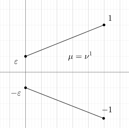
(a) $\mu=\nu^{1}$

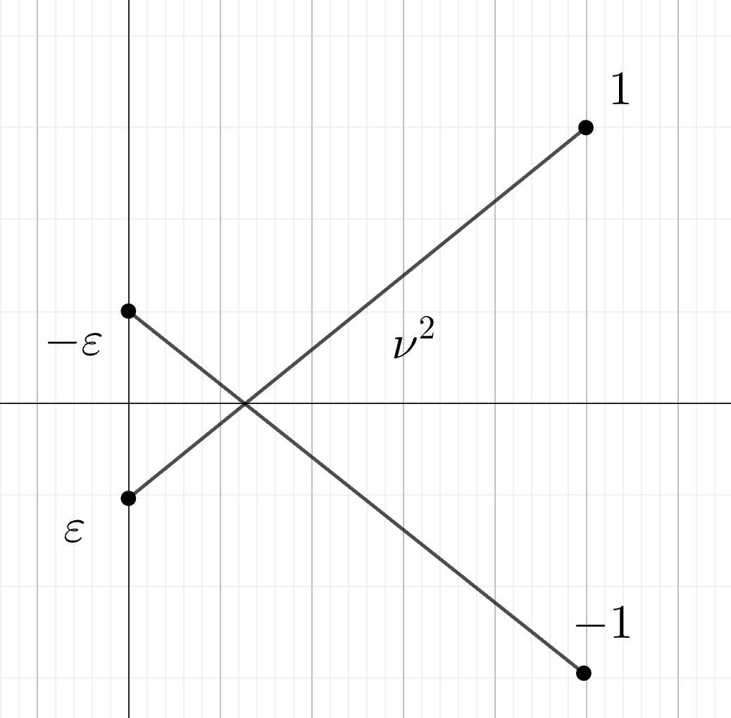
(b) $\nu^{2}$

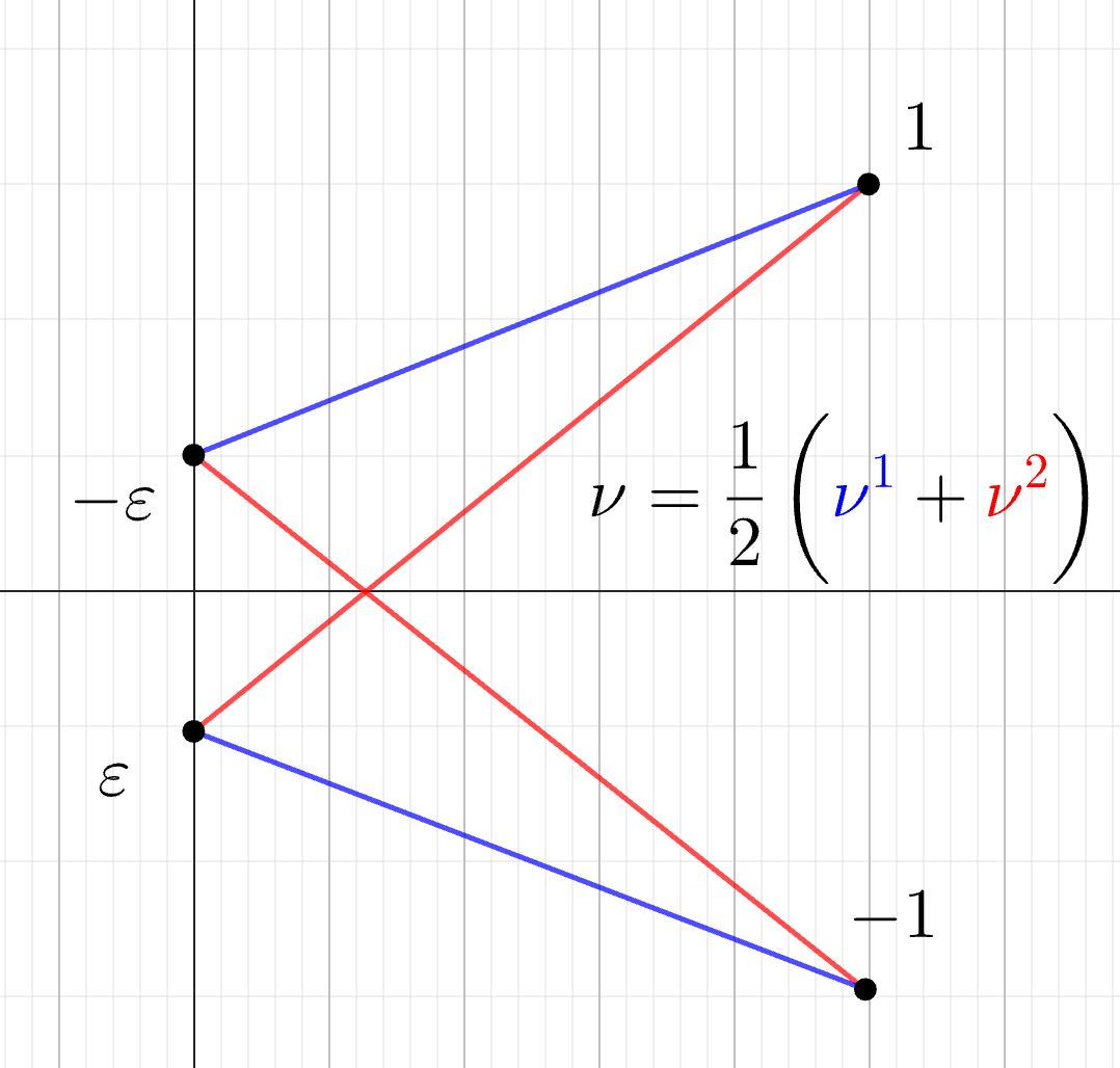
(c) $\nu$

Figure 2: Visualization of $\mu,\nu^{1},\nu^{2}$ and $\nu$.

see Figure 2 for visualization. Then we have

$$\mathcal{AW}_{1}(\mu,\nu^{1})=0,\quad\mathcal{AW}_{1}(\mu,\nu^{2})=2\epsilon,\quad\mathcal{AW}_{1}(\mu,\nu)=1.$$

By choosing $\epsilon<1$, we have

$$\mathcal{AW}_{1}(\mu,\nu)=1>\epsilon=\frac{1}{M}\sum_{m=1}^{M}\mathcal{AW}_{1}(\mu,\nu^{m}).$$

References

• [ABP22] Beatrice Acciaio, Julio Backhoff and Gudmund Pammer “Quantitative fundamental theorem of asset pricing” In arXiv preprint arXiv:2209.15037, 2022
• [ABZ20] Beatrice Acciaio, Julio Backhoff-Veraguas and Anastasiia Zalashko “Causal optimal transport and its links to enlargement of filtrations and continuous-time stochastic optimization” In Stochastic Processes and their Applications 130.5 Elsevier, 2020, pp. 2918–2953
• [AH22] Beatrice Acciaio and Songyan Hou “Convergence of Adapted Empirical Measures on $\mathbb{R}^{d}$ In arXiv preprint arXiv:2211.10162, 2022
• [Bac+22] Julio Backhoff, Daniel Bartl, Mathias Beiglböck and Johannes Wiesel “Estimating processes in adapted Wasserstein distance” In The Annals of Applied Probability 32.1 Institute of Mathematical Statistics, 2022, pp. 529–550
• [Bac+19] Julio Backhoff-Veraguas, Daniel Bartl, Mathias Beiglböck and Manu Eder “All adapted topologies are equal” In Probability Theory and Related Fields 178, 2019, pp. 1125–1172
• [Bac+20] Julio Backhoff-Veraguas, Daniel Bartl, Mathias Beiglböck and Manu Eder “Adapted Wasserstein distances and stability in mathematical finance” In Finance and Stochastics 24 Springer, 2020, pp. 601–632
• [Bac+17] Julio Backhoff-Veraguas, Mathias Beiglbock, Yiqing Lin and Anastasiia Zalashko “Causal transport in discrete time and applications” In SIAM Journal on Optimization 27.4 SIAM, 2017, pp. 2528–2562
• [BW23] Daniel Bartl and Johannes Wiesel “Sensitivity of Multiperiod Optimization Problems with Respect to the Adapted Wasserstein Distance” In SIAM Journal on Financial Mathematics, 2023
• [BT19] Jocelyne Bion–Nadal and Denis Talay “On a Wasserstein-type distance between solutions to stochastic differential equations” In The Annals of Applied Probability 29.3 Institute of Mathematical Statistics, 2019, pp. 1609–1639
• [BG10] Sergey G. Bobkov and Friedrich Gotze “Concentration of empirical distribution functions with applications to non-i.i.d. models” In Bernoulli 16, 2010, pp. 1385–1414
• [BL14] Emmanuel Boissard and Thibaut Le Gouic “On the mean speed of convergence of empirical and occupation measures in Wasserstein distance” In Annales de l’IHP Probabilités et statistiques 50.2, 2014, pp. 539–563
• [BGV07] François Bolley, Arnaud Guillin and Cédric Villani “Quantitative concentration inequalities for empirical measures on non-compact spaces” In Probability Theory and Related Fields 137 Springer, 2007, pp. 541–593
• [BY78] Pierre Brémaud and Marc Yor “Changes of filtrations and of probability measures” In Zeitschrift für Wahrscheinlichkeitstheorie und verwandte Gebiete 45.4 Springer, 1978, pp. 269–295
• [DSS13] Steffen Dereich, Michael Scheutzow and Reik Schottstedt “Constructive quantization: Approximation by empirical measures” In Annales de l’IHP Probabilités et statistiques 49.4, 2013, pp. 1183–1203
• [Dud69] Richard Mansfield Dudley “The speed of mean Glivenko-Cantelli convergence” In The Annals of Mathematical Statistics 40.1 JSTOR, 1969, pp. 40–50
• [Dug51] James Dugundji “An extension of Tietze’s theorem.” In Pacific Journal of Mathematics 1.3, 1951, pp. 353–367
• [Fou22] Nicolas Fournier “Convergence of the empirical measure in expected Wasserstein distance: non asymptotic explicit bounds in Rd” In ESAIM: Probability and Statistics, 2022
• [FG15] Nicolas Fournier and Arnaud Guillin “On the rate of convergence in Wasserstein distance of the empirical measure” In Probability Theory and Related Fields 162.3 Springer, 2015, pp. 707–738
• [Gig08] Nicola Gigli “On the geometry of the space of probability measures in Rn endowed with the quadratic optimal transport distance”, 2008
• [GN21] Evarist Giné and Richard Nickl “Mathematical foundations of infinite-dimensional statistical models” Cambridge university press, 2021
• [Gol+20] Ziv Goldfeld, Kristjan Greenewald, Jonathan Niles-Weed and Yury Polyanskiy “Convergence of smoothed empirical measures with applications to entropy estimation” In IEEE Transactions on Information Theory 66.7 IEEE, 2020, pp. 4368–4391
• [GG20] Ziv Goldfeld and Kristjan H. Greenewald “Gaussian-Smoothed Optimal Transport: Metric Structure and Statistical Efficiency” In AISTATS, 2020
• [Las18] Rémi Lassalle “Causal transference plans and their Monge-Kantorovich problems” In Stochastic Processes and their Applications 36.3 Elsevier, 2018, pp. 452–484
• [Lei18] Jing Lei “Convergence and concentration of empirical measures under Wasserstein distance in unbounded functional spaces” In Bernoulli, 2018
• [McD89] Colin McDiarmid “On the method of bounded differences” In Surveys in combinatorics 141.1 Norwich, 1989, pp. 148–188
• [Pam22] Gudmund Pammer “A note on the adapted weak topology in discrete time” In arXiv preprint arXiv:2205.00989, 2022
• [PP12] Georg Ch Pflug and Alois Pichler “A distance for multistage stochastic optimization models” In SIAM Journal on Optimization 22.1 SIAM, 2012, pp. 1–23
• [PP14] Georg Ch Pflug and Alois Pichler “Multistage stochastic optimization” Springer, 2014
• [PP16] Georg Ch Pflug and Alois Pichler “From empirical observations to tree models for stochastic optimization: convergence properties” In SIAM Journal on Optimization 26.3 SIAM, 2016, pp. 1715–1740
• [Rüs85] Ludger Rüschendorf “The Wasserstein distance and approximation theorems” In Probability Theory and Related Fields 70.1 Springer, 1985, pp. 117–129
• [WB19] Jonathan Weed and Francis Bach “Sharp asymptotic and finite-sample rates of convergence of empirical measures in Wasserstein distance” In Bernoulli 25.4A Bernoulli Society for Mathematical StatisticsProbability, 2019, pp. 2620–2648