Data-Enabled Policy Optimization for Direct Adaptive Learning of the LQR

Abstract

Direct data-driven design methods for the linear quadratic regulator (LQR) mainly use offline or episodic data batches, and their online adaptation has been acknowledged as an open problem. In this paper, we propose a direct adaptive method to learn the LQR from online closed-loop data. First, we propose a new policy parameterization based on the sample covariance to formulate a direct data-driven LQR problem, which is shown to be equivalent to the certainty-equivalence LQR with optimal non-asymptotic guarantees. Second, we design a novel data-enabled policy optimization (DeePO) method to directly update the policy, where the gradient is explicitly computed using only a batch of persistently exciting (PE) data. Third, we establish its global convergence via a projected gradient dominance property. Importantly, we efficiently use DeePO to adaptively learn the LQR by performing only one-step projected gradient descent per sample of the closed-loop system, which also leads to an explicit recursive update of the policy. Under PE inputs and for bounded noise, we show that the average regret of the LQR cost is upper-bounded by two terms signifying a sublinear decrease in time $\mathcal{O}(1/\sqrt{T})$ plus a bias scaling inversely with signal-to-noise ratio (SNR), which are independent of the noise statistics. Finally, we perform simulations to validate the theoretical results and demonstrate the computational and sample efficiency of our method.

I Introduction

As a cornerstone of modern control theory, the linear quadratic regulator (LQR) design has been widely studied in data-driven control, where no model but only raw data is available [1]. The manifold approaches to data-driven LQR design can be broadly categorized as indirect, i.e., based on offline system identification (SysID) followed by model-based control design, versus direct when bypassing the identification step. Another classification is episodic when obtaining the policy from single or multiple alternating episodes of data collection and control (see Fig. 1), versus adaptive when updating the policy from online closed-loop data (see Fig. 2).

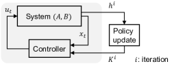
Figure 1: An illustration of episodic approaches, where $h^{i}=(x_{0},u_{0},\dots,x_{T^{i}})$ denotes the trajectory of the $i$-th episode.

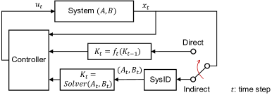
Figure 2: An illustration of indirect and direct adaptive approaches in closed-loop, where $f_{t}$ is some explicit function.

The indirect data-driven LQR design has a rich history and has developed well-understood tools for identification and control. Representative approaches include [2] advocating optimism-in-face-of-uncertainty, [3] in the robust setting, and [4, 5, 6, 7, 8] based on certainty-equivalence control. Most of them are episodic in that they either estimate the system dynamics from a single episode of offline data, or update their estimate only after an episode is completed [2, 3, 4, 5]. This is due to their requirement of statistically independent data and regret analysis methods. Notable adaptive methods are [6, 7, 8] rooted on certainty-equivalence LQR: a system is first identified by ordinary least-squares from closed-loop data, and then a certainty-equivalence LQR problem is solved by treating the estimated system as the ground-truth [4]. By alternating identification and certainty-equivalence LQR, they guarantee convergence to the optimal LQR gain. In particular, the work [6] takes the first step towards indirect adaptive control with asymptotic convergence guarantees by regularizing the identification objective with the LQR cost. Recent works [7, 8] have shown that certainty-equivalence control with explorative input ensuring persistency of excitation meets optimal non-asymptotic guarantees, i.e., the LQR gain converges at a sublinear rate. However, the indirect adaptive approach requires solving an algebraic Riccati equation per time, which is computationally demanding and lacks a recursive policy update.

Instead of solving an algebraic Riccati equation with the identified model, an emerging line of direct methods obtains the LQR directly from a single episode of persistently exciting (PE) data [9, 10, 11, 12, 13]. It is inspired by subspace methods [14] and the fundamental lemma [15] in behavioral system theory [16, 17, 18, 19]. Using subspace relations, the works [9, 10, 11] show that the closed-loop system can be parameterized by state-space data, leading to direct data-driven formulations of the LQR problem. By a standard change of variables, they can be reformulated as semi-definite programs (SDPs) parameterized by raw data matrices. In the presence of noise, regularization methods are introduced for direct LQR design to promote certainty-equivalence or robustness [11, 12, 13]. There are also works [20, 21] developing matrix S-lemma or combining prior knowledge for robust LQR design, while they are inherently conservative. All these methods are based on a single episode of offline data, and the dimension of their formulations usually scales with data length. Since adaptation of the policy to the latest data may not improve the performance, they cannot use online closed-loop data to achieve adaptive learning of the LQR. In fact, their real-time adaptation is a fundamental open problem in the data-driven control field [16, 14, 22].

A possible path to direct and online adaptive control is policy optimization (PO), a direct design framework where the policy is parameterized and recursively updated to minimize a cost function. Dating back to the adaptive control of aircraft in the 1950s [23], the concept of direct PO has a long history in control theory [24, 25, 26]. However, due to the non-convexity of PO formulations, it is usually challenging to obtain strong performance guarantees. Recently, there have been resurgent interests in studying theoretical properties of zeroth-order PO, an essential approach of modern reinforcement learning [27, 28, 29, 30, 31, 32]. It improves the policy by gradient methods, where the gradient is estimated from observations of the cost. For the LQR problem, zeroth-order PO meets global linear convergence thanks to a gradient dominance property [27, 28, 29]. However, zeroth-order PO is intrinsically unsuitable for adaptive control since 1) the cost used for gradient estimate can be obtained only after observing an entire trajectory, 2) the trajectory needs to be sufficiently long to reduce the estimation error, and 3) it requires numerous trajectories to find an optimal policy. Different from zeroth-order PO, our recent work [33] has proposed a data-enabled PO (DeePO) method for the LQR, where the gradient is computed directly from a single trajectory of finite length, and shown global convergence. This is achieved by adopting the data-based policy parameterization in [10, 11, 12, 13]. While this DeePO method is based on offline data, it paves the way to applying PO for direct and online adaptive control.

Following [33], this paper proposes a novel DeePO method for direct adaptive learning of the LQR, where the policy is directly updated by gradient methods from online closed-loop data; see Fig. 2. Hence, we provide a promising solution to the open problem in [16, 14, 22].

One of our main contributions is a new policy parameterization for the LQR based on the sample covariance, which is a key ingredient in SysID [4], filtering [34], and data-driven control parameterizations [35, 19, 36]. Compared with the existing parameterization [10, 11, 12, 13], it has two salient features that enable online adaptation of DeePO. First, the dimension of the parameterized policy is a constant depending only on the system dimension. Second, the resulting direct LQR is shown to be equivalent to the indirect certainty-equivalence LQR, which usually requires regularized direct formulations and methods [11, 12, 13]. In view of [4, 5], this equivalence implies that our covariance parameterization is efficient in using data.

Based on the covariance parameterization of the policy, we first show the convergence of DeePO for the LQR. While the covariance-parameterized LQR problem is non-convex and has a subspace constraint, we show that a key projected gradient dominance property holds. In conjunction with the local smoothness of the LQR cost, we show that projected gradient descent achieves global convergence. Then, we use DeePO to adaptively learn the LQR gain, while performing only a single projected gradient step per time using online closed-loop data. It leads to an explicit recursive update of the policy and has negligible real-time computation cost compared to the indirect adaptive approach [6, 7, 8].

We provide non-asymptotic guarantees of DeePO for adaptive learning of the LQR. Under a quantitative condition of PE inputs and bounded process noise, the average regret of the LQR cost is upper-bounded by two terms signifying a sublinear decrease in time $\mathcal{O}(1/\sqrt{T})$ plus a bias scaling inversely as signal-to-noise ratio (SNR), which are independent of the noise statistics. It improves over single batch methods [11, 12, 13], whose performance also depends on SNR but does not decay over time. Our sublinear decrease rate aligns with that of first-order methods in online convex optimization of smooth functions [37, Chapter 3], even though our considered LQR problem is non-convex. This astonishing rate shows the sample efficiency of DeePO to learn from online closed-loop data.

In the simulation, we validate the convergence of DeePO for learning the LQR using offline and online closed-loop data, respectively. Moreover, we compare DeePO with the indirect adaptive approach [6, 7, 8] and zeroth-order PO [27, 29, 28] over a benchmark problem in [3]. The simulations show the superior computational and sample efficiency of our method.

The rest of this paper is organized as follows. Section II recapitulates data-driven LQR formulations and describes the adaptive learning problem. Section III proposes the covariance parameterization for the LQR. Section IV uses DeePO to solve LQR parameterization with offline data. Section V extends DeePO to direct adaptive learning of the LQR with non-asymptotic guarantees. Section VI validates our theoretical results via simulations. We provide concluding remarks in Section VII. All the proofs are deferred to the Appendices.

Notation. We use $I_{n}$ to denote the $n$-by-$n$ identity matrix. We use $\underline{\sigma}(\cdot)$ to denote the minimal singular value of a matrix. We use $\|\cdot\|$ to denote the $2$-norm of a vector or matrix, and $\|\cdot\|_{F}$ the Frobenius norm. We use $\rho(\cdot)$ to denote the spectral radius of a square matrix. We use $A^{\dagger}:=A^{\top}(AA^{\top})^{-1}$ to denote the right inverse of a full row rank matrix $A\in\mathbb{R}^{n\times m}$. We use $\mathcal{N}(A)$ to denote the nullspace of $A$ and $\Pi_{A}:=I_{m}-A^{\dagger}A$ the projection operator onto it.

II Data-driven formulations and adaptive learning of the LQR

In this section, we first recapitulate indirect certainty-equivalence LQR (least-square SysID followed by model-based LQR design), direct LQR design using data-based policy parameterization, and policy optimization (PO) of the LQR based on zeroth-order gradient estimate. Then, we formalize our adaptive learning problem.

II-A Model-based LQR

Consider a discrete-time linear time-invariant system

$$x_{t+1}=Ax_{t}+Bu_{t}+w_{t},$$ (1)

where $t\in\mathbb{N}$, $x_{t}\in\mathbb{R}^{n}$ is the state, $u_{t}\in\mathbb{R}^{m}$ is the control input, $w_{t}\in\mathbb{R}^{n}$ is the noise, and $(A,B)$ is controllable.

The LQR problem is phrased as finding a state-feedback gain $K\in\mathbb{R}^{m\times n}$ to minimize the quadratic cost

$$\limsup_{T\rightarrow\infty}\mathbb{E}_{\{w_{t}\}}\left[\frac{1}{T}\sum_{t=0}^{T-1}(x_{t}^{\top}Qx_{t}+u_{t}^{\top}Ru_{t})\right],$$

where $Q\succ 0$, $R\succ 0$, and $\{x_{t},u_{t}\}$ is the trajectory following $u_{t}=Kx_{t}$ starting from an initial state $x_{0}$.

When $A+BK$ is stable and $\{w_{t}\}$ is a white process with zero mean and unit covariance, the cost can be written as [27]

$$C(K):=\text{Tr}\left((Q+K^{\top}RK)\Sigma_{K}\right),$$ (2)

where $\Sigma_{K}$ is the closed-loop state covariance matrix obtained as the positive definite solution to the Lyapunov equation

$$\Sigma_{K}=I_{n}+(A+BK)\Sigma_{K}(A+BK)^{\top}.$$ (3)

We refer to (2)-(3) as a policy parameterization of the LQR.

There are alternative formulations to find the optimal LQR gain $K^{*}$ of (2)-(3), e.g., via the celebrated Riccati equation with known $(A,B)$ [1]. For unknown $(A,B)$, there is a plethora of data-driven control methods to find $K^{*}$, some of which we recapitulate below.

II-B Indirect certainty-equivalence LQR with ordinary least-square identification

This conventional approach to data-driven LQR design first identifies a system $(A,B)$ from data, and then solves the LQR problem regarding the identified model as the ground-truth. The SysID step is based on subspace relations among the state-space data. Consider the $t$-long time series of states, inputs, noises, and successor states

$$X_{0} :=\begin{bmatrix}x_{0}&x_{1}&\dots&x_{t-1}\end{bmatrix}\in\mathbb{R}^{n\times t},$$ (4)

$$U_{0} :=\begin{bmatrix}u_{0}&u_{1}&\dots&u_{t-1}\end{bmatrix}\in\mathbb{R}^{m\times t},$$

$$W_{0} :=\begin{bmatrix}w_{0}&w_{1}&\dots&w_{t-1}\end{bmatrix}\in\mathbb{R}^{n\times t},$$

$$X_{1} :=\begin{bmatrix}x_{1}&x_{2}&\dots&x_{t}\end{bmatrix}\in\mathbb{R}^{n\times t},$$

which satisfy the system dynamics

$$X_{1}=AX_{0}+BU_{0}+W_{0}.$$ (5)

We assume that the data is persistently exciting (PE) [15], i.e., the block matrix of input and state data

$$D_{0}:=\begin{bmatrix}U_{0}\\ X_{0}\end{bmatrix}\in\mathbb{R}^{(m+n)\times T}$$

has full row rank

$$\text{rank}(D_{0})=m+n.$$ (6)

This PE condition is mild and necessary for the data-driven LQR design [38, 39].

Based on the subspace relations (5) and the rank condition (6), an estimate $(\hat{A},\hat{B})$ of the system can be obtained as the unique solution to the ordinary least-squares problem

$$[\hat{B},\hat{A}]=\underset{B,A}{\arg\min}\left\|X_{1}-[B,A]D_{0}\right\|_{F}=X_{1}D_{0}^{\dagger}.$$ (7)

Following the certainty-equivalence principle [12], the system $(A,B)$ is replaced with its estimate $(\hat{A},\hat{B})$ in (2)-(3), and the LQR problem can be reformulated as a bi-level program

$$\mathop{\text{minimize}}\limits_{K,\Sigma\succeq 0}{}{} \text{Tr}\left((Q+K^{\top}RK)\Sigma\right),$$ (8)

subject to $$\Sigma=I_{n}+(\hat{A}+\hat{B}K)\Sigma(\hat{A}+\hat{B}K)^{\top}$$

$$[\hat{B},\hat{A}]=\underset{B,A}{\arg\min}\left\|X_{1}-[B,A]W_{0}\right\|_{F}.$$

The problem (8) is termed certainty-equivalence and indirect data-driven LQR design in [13]. By alternating between solving (8) and using the resulting policy to collect online closed-loop data, it achieves adaptive learning of the LQR with optimal non-asymptotic guarantees [7, 8]. However, it is computationally demanding to solve (8) per time and a recursive policy update is absent.

II-C Direct LQR design with data-based policy parameterization

In contrast to the SysID-followed-by-control approach (8), the direct data-driven LQR design aims to find $K^{*}$ bypassing the identification step (7). It uses a data-based policy parameterization: by the rank condition (6), there exists a matrix $G\in\mathbb{R}^{T\times n}$ that satisfies

$$\begin{bmatrix}K\\ I_{n}\end{bmatrix}=D_{0}G$$ (9)

for any given $K$. Together with the subspace relations (5), the closed-loop matrix can be written as

$$A+BK=[B,A]\begin{bmatrix}K\\ I_{n}\end{bmatrix}\overset{\eqref{equ:relation}}{=}[B,A]D_{0}G\overset{\eqref{equ:dynamics}}{=}(X_{1}-W_{0})G,$$

Since $W_{0}$ is unknown and unmeasurable, it is disregarded and $X_{1}G$ is used as the closed-loop matrix. Following the certainty-equivalence principle [12], we substitute $A+BK$ with $X_{1}G$ in (2)-(3), and together with (9) the LQR problem becomes

$$\mathop{\text{minimize}}\limits_{G,\Sigma\succeq 0}~{}\text{Tr}\left((Q+G^{\top}U_{0}^{\top}RU_{0}G)\Sigma\right),$$ (10)

$$\text{subject to}~{}~{}\Sigma=I_{n}+X_{1}G\Sigma G^{\top}X_{1}^{\top},~{}X_{0}G=I_{n}$$

with the gain matrix $K=U_{0}G$, which can be reformulated as an SDP [10]. The LQR parameterization (10) is direct data-driven, as it does not involve any explicit SysID.

However, the dimension of the LQR parameterization (10) scales linearly with $t$, and it is unclear how to turn (10) into a recursive formulation suited for online closed-loop adaptation.

II-D PO of the LQR using zeroth-order gradient estimate

As an essential approach of modern reinforcement learning, zeroth-order PO finds $K^{*}$ by iterating the gradient descent [27, 29, 28] for the policy parameterization of the LQR (2)-(3):

$$K^{\prime}=K-\eta\widehat{\nabla C(K)}.$$ (11)

The PO (11) is initialized with a stabilizing gain, $\eta>0$ is a constant stepsize, and $\widehat{\nabla C(K)}$ is the gradient estimate from zeroth-order information. For example, the two-point gradient estimate is given by

$$\widehat{\nabla C(K)}=\left(\hat{C}(K+rF)-\hat{C}(K-rF)\right)\cdot\frac{mn}{r}F,$$ (12)

where the constant $r>0$ is the smoothing radius, $F$ is uniformly sampled from the unit sphere $\mathbb{S}^{mn-1}$, and $\hat{C}$ is the approximated cost observed from a $T$-long trajectory of system (1), i.e., $\hat{C}(K)=\frac{1}{T}\sum_{t=0}^{T-1}(x_{t}^{\top}Qx_{t}+u_{t}^{\top}Ru_{t})$ with $u_{t}=Kx_{t}$.

While zeroth-order PO has a recursive policy update, it requires to sample numerous long trajectories to find $K^{*}$, which is inherently unsuitable for online adaptive control.

II-E Direct adaptive learning for the LQR with online closed-loop data

All the aforementioned data-driven LQR design methods either lack a recursive policy update, or are unsuitable for adaptive control with online closed-loop data. In this paper, we focus on the direct adaptive learning problem of the LQR:

Problem: design a recursive direct method based on online closed-loop data such that the control policy converges to the optimal LQR gain.

Following [10, 11, 12, 13], we start with a direct data-driven LQR formulation but with a new policy parameterization that enables efficient use of data. Then, we take an iterative PO perspective to the direct data-driven LQR as in our previous work [33], and use projected gradient methods to achieve adaptive learning of the LQR using online closed-loop data.

III Direct data-driven LQR with a new policy parameterization

In this section, we first propose a new policy parameterization based on the sample covariance to formulate the direct data-driven LQR problem. Then, we establish its equivalence to the indirect certainty-equivalence LQR problem.

III-A A new policy parameterization using sample covariance

To efficiently use data, we propose a new policy parameterization based on the sample covariance of input-state data

$$\Lambda:=\frac{1}{t}D_{0}D_{0}^{\top}=\frac{1}{t}\begin{bmatrix}U_{0}\\ X_{0}\end{bmatrix}\begin{bmatrix}U_{0}\\ X_{0}\end{bmatrix}^{\top},$$ (13)

which plays an important role in SysID [4], filtering [34], and data-driven control parameterizations [35, 19, 36]. Under the PE rank condition (6), the sample covariance $\Lambda$ is positive definite, and there exists a unique solution $V\in\mathbb{R}^{(n+m)\times n}$ to

$$\begin{bmatrix}K\\ I_{n}\end{bmatrix}=\Lambda V$$ (14)

for any given $K$. We refer to (14) as the covariance parameterization of the policy. In contrast to the parameterization in (9), the dimension of $V$ here is independent of the data length.

Remark 1

The covariance parameterization (14) can also be derived from (9). Since $D_{0}$ does not necessarily have full column rank, there is a considerable nullspace in the solution of (9), which can be reparameterized via orthogonal decomposition:

$$G=\frac{1}{t}D_{0}^{\top}V+\Delta,\Delta\in\mathcal{N}(D_{0})$$ (15)

with $V\in\mathbb{R}^{(n+m)\times n}$. If we remove the nullspace $\mathcal{N}(D_{0})$ in (15), then the parameterization (9) reduces to (14). We note that the nullspace is undesirable, and regularization methods have to be used to single out a solution[11, 12, 13].  

For brevity, let

$$\overline{X}_{0}=\frac{1}{t}X_{0}D_{0}^{\top},\overline{U}_{0}=\frac{1}{t}U_{0}D_{0}^{\top},$$

$$\overline{W}_{0}=\frac{1}{t}W_{0}D_{0}^{\top},\overline{X}_{1}=\frac{1}{t}X_{1}D_{0}^{\top}.$$

Then, the closed-loop matrix can be written as

$$A+BK=[B,A]\begin{bmatrix}K\\ I_{n}\end{bmatrix}\overset{\eqref{equ:newpara}}{=}[B,A]\Lambda V\overset{\eqref{equ:dynamics}}{=}(\overline{X}_{1}-\overline{W}_{0})V.$$ (16)

Analogously to (10), we disregard the uncertainty $\overline{W}_{0}$ in the parameterized closed-loop matrix and formulate the direct data-driven LQR problem using $(X_{0},U_{0},X_{1})$ as

$$\mathop{\text{minimize}}\limits_{V,\Sigma_{V}\succeq 0}~{}J(V):=\text{Tr}\left((Q+V^{\top}\overline{U}_{0}^{\top}R\overline{U}_{0}V)\Sigma_{V}\right),$$ (17)

$$\text{subject to}~{}~{}\Sigma_{V}=I_{n}+\overline{X}_{1}V\Sigma_{V}V^{\top}\overline{X}_{1}^{\top},\overline{X}_{0}V=I_{n}$$

with the gain matrix $K=\overline{U}_{0}V$. We refer to (17) as the LQR problem with covariance parameterization.

III-B The equivalence between the covariance parameterization of the LQR and the indirect certainty-equivalence LQR

We now show that the data-driven covariance parameterization (17) is equivalent to the indirect certainty-equivalence LQR (8) in the sense that their solutions coincide. Let $J^{*}$ and $C_{\text{CE}}^{*}$ be the optimum of (17) and (8), respectively. Then, we have the following result.

Lemma 1 (Equivalence to the certainty-equivalence LQR)

The feasible sets of (17) and (8) coincide under the change of variables $V=\Lambda^{-1}[K^{\top},I_{n}]^{\top}$, and their optimum is equal, i.e., $J^{*}=C_{\text{CE}}^{*}$.

Remark 2 (Implicit regularization)

This equivalence has also been shown for the LQR parameterization (10) with a sufficiently large certainty-equivalence regularizer, i.e.,

$$\mathop{\text{minimize}}\limits_{G,\Sigma\succeq 0}~{}\text{Tr}\left((Q+G^{\top}U_{0}^{\top}RU_{0}G)\Sigma\right)+\lambda\|\Pi_{D_{0}}G\|,$$ (18)

$$\text{subject to}~{}~{}\Sigma=I_{n}+X_{1}G\Sigma G^{\top}X_{1}^{\top},~{}X_{0}G=I_{n}$$

with the gain $K=U_{0}G$ [12, Corollary 3.2]. Thus, the covariance parametrization of the LQR (17) is implicitly regularized as it achieves this equivalence without any regularization. An implicit regularization property is also observed in the PO of (18) in the absence of noise [33, Theorem 2].  

While the LQR problem with covariance parameterization (17) can be reformulated as an SDP as in [10, 11, 12, 13], our subsequent solution will not make use of that. Instead, the next section solves (17) via an iterative PO method with convergence guarantees.

IV DeePO for the LQR with covariance parameterization using offline data

In this section, we first present our novel PO method to solve the LQR problem with covariance parameterization (17) given offline data $(X_{0},U_{0},X_{1})$. Then, we show its global convergence by proving a projected gradient dominance property.

IV-A Data-enabled policy optimization to solve the LQR problem with covariance parameterization (17)

Define the feasible set of (17) as

$$\mathcal{S}:=\{V\mid\overline{X}_{0}V=I_{n},\rho(\overline{X}_{1}V)<1\},$$

which is assumed to be non-empty. Since it contains a subspace constraint $\overline{X}_{0}V=I_{n}$, we use projected gradient methods to solve (17) while maintaining feasibility.

We first derive the gradient for $J(V)$. Since $\Sigma_{V}=\sum_{i=0}^{\infty}(\overline{X}_{1}V)^{i}(V^{\top}\overline{X}_{1}^{\top})^{i}$, the cost $J(V)$ can be expressed as

$$J(V) =\text{Tr}\left((Q+V^{\top}\overline{U}_{0}^{\top}R\overline{U}_{0}V)\sum_{i=0}^{\infty}(\overline{X}_{1}V)^{i}(V^{\top}\overline{X}_{1}^{\top})^{i}\right)$$

$$=\text{Tr}\left(\sum_{i=0}^{\infty}(V^{\top}\overline{X}_{1}^{\top})^{i}(Q+V^{\top}\overline{U}_{0}^{\top}R\overline{U}_{0}V)(\overline{X}_{1}V)^{i}\right)$$

$$=\text{Tr}(P_{V}),$$ (19)

where $P_{V}$ satisfies the Lyapunov equation

$$P_{V}=Q+V^{\top}\overline{U}_{0}^{\top}R\overline{U}_{0}V+V^{\top}\overline{X}_{1}^{\top}P_{V}\overline{X}_{1}V.$$ (20)

Then, the closed-form expression for $\nabla J(V)$ is as follows.

Lemma 2

For $V\in\mathcal{S}$, the gradient of $J(V)$ is

$$\nabla J(V)=2\left(\overline{U}_{0}^{\top}R\overline{U}_{0}+\overline{X}_{1}^{\top}P_{V}\overline{X}_{1}\right)V\Sigma_{V}.$$

By Lemma 2, the gradient can be computed directly from raw data matrices. Starting from a feasible $V^{0}\in\mathcal{S}$, the projected gradient method iterates as

$$V^{k+1}=V^{k}-\eta\Pi_{\overline{X}_{0}}\nabla J(V^{k}),~{}k\in\mathbb{N},$$ (21)

where $\eta\geq 0$ is a constant stepsize, and the projection $\Pi_{\overline{X}_{0}}$ enforces the subspace constraint $\overline{X}_{0}V=I_{n}$. We refer to (21) as data-enabled policy optimization (DeePO) since the projected gradient is data-driven, and the control gain can be recovered from the covariance parameterization (14) as $K=\overline{U}_{0}V$.

Due to non-convexity of the considered problem (19)-(20), it is challenging to provide convergence guarantees for DeePO in (21). The existing PO methods achieve global convergence for the LQR by leveraging a gradient dominance property[27, 29, 28], which is a weaker condition than strong convexity. Here, we show a similar projected gradient dominance property of $J(V)$, as a key to global convergence within $\mathcal{S}$.

IV-B Projected gradient dominance of the LQR cost

We first define the projected gradient dominance property.

Definition 1 (Projected gradient dominance)

A continuously differentiable function $g(x):\mathbb{R}^{n}\rightarrow\mathbb{R}$ is projected gradient dominated of degree $p\in\{1,2\}$ over a subset $\mathcal{X}\subseteq\text{dom}(g)$ if

$$g(x)-g(x^{*})\leq\alpha\|\Pi\nabla g(x)\|^{p},~{}~{}\forall x\in\mathcal{X},$$

where $\alpha>0$ is a constant, $x^{*}$ is an optimal solution of $g(x)$ over $\mathcal{X}$, and $\Pi$ is a projection onto a subset of $\mathcal{X}$.

In comparison to the definition of gradient dominance [32, Definition 1], Definition 1 focuses on the property of the projected gradient, meaning that optimality is achieved when the projected gradient attains zero. It leads to global convergence of projected gradient descent in conjuncture with a smoothness property, and the convergence rate depends on the degree $p$. In particular, for smooth objective $p=1$ leads to a sublinear rate and $p=2$ leads to a linear rate.

For problem (19)-(20), we show that $J(V)$ is projected gradient dominated of degree 1 over any sublevel set $\mathcal{S}(a):=\{V\in\mathcal{S}\mid J(V)\leq a\}$ with $a>0$, the proof of which leverages [40, Theorem 1] and a convex reparameterization.

Lemma 3 (Projected gradient dominance of degree 1)

For $V\in\mathcal{S}(a)$, it holds that

$$J(V)-J^{*}\leq\mu(a)\|\Pi_{\overline{X}_{0}}\nabla J(V)\|,$$

with $\mu(a):={4a^{2}}/\left({(\underline{\sigma}(Q))^{{3}/{2}}(\underline{\sigma}(R))^{{1}/{2}}\underline{\sigma}(\overline{U}_{0})}\right).$

Armed with Lemma 3, we show the global convergence of the projected gradient descent (21) in the next subsection.

IV-C Global convergence of DeePO

As in the LQR parameterization (2)-(3), the cost $J(V)$ here tends to infinity as $V$ approaches the boundary $\partial\mathcal{S}$ [27]. Thus, it is only locally smooth over a sublevel set.

Lemma 4 (Local smoothness)

For any $V,V^{\prime}\in\mathcal{S}(a)$ satisfying $V+\phi(V^{\prime}-V)\in\mathcal{S}(a)$ for all scalar $\phi\in[0,1]$, it holds that

$$J(V^{\prime})\leq J(V)+\langle\nabla J(V),V^{\prime}-V\rangle+{l(a)}\|V^{\prime}-V\|^{2}/2,$$

where the smoothness constant is given by

$$l(a):=4a^{2}\left(\xi(a)+a-\underline{\sigma}(Q)\right)\frac{\|\overline{X}_{1}\|_{F}^{2}}{\underline{\sigma}^{2}(Q)}+\frac{2\xi(a)a}{\underline{\sigma}(Q)}$$

with $\xi(a):=\|\overline{U}_{0}\|^{2}\|R\|+\|\overline{X}_{1}\|^{2}a$.

While Lemmas 3 and 4 are local properties over a sublevel set, we can use them as global ones by selecting an appropriate stepsize such that the policy sequence stays in this sublevel set. For brevity, let $\mu^{0}:=\mu(J(V^{0}))$ and $l^{0}:=l(J(V^{0}))$, where $V^{0}\in\mathcal{S}$ is an initial policy. The convergence of DeePO in (21) is shown as follows.

Theorem 1 (Global convergence)

For $V^{0}\in\mathcal{S}$ and a stepsize $\eta\in(0,1/l^{0}]$, the projected gradient descent (21) leads to $V^{k}\in\mathcal{S}(J(V^{0})),\forall k\in\mathbb{N}$. Moreover, for any $\epsilon>0$ and

$$k\geq\frac{2(\mu^{0})^{2}}{\epsilon(2\eta-l^{0}\eta^{2})},$$ (22)

the update (21) meets the following performance bound

$$J(V^{k})-J^{*}\leq\epsilon.$$

We compare our DeePO method developed thus far with zeroth-order PO in (11)-(12) [27, 28, 29]. Since $J(V)$ is projected gradient dominated of degree 1, we have shown sublinear convergence of projected gradient descent to $J^{*}$. In comparison, $C(K)$ in (2) is gradient dominated of degree 2 [27], and hence zeroth-order PO meets linear convergence to $C^{*}:=\min_{K}C(K)$. However, they rely on zeroth-order gradient estimates, which inevitably require numerous and long trajectories. In contrast, DeePO efficiently computes the gradient from a batch of raw and PE data matrices based on the covariance parameterization of the LQR (17). This remarkable feature enables DeePO to utilize online closed-loop data for adaptive control with recursive updates, as shown in the next section.

V DeePO for direct, adaptive, and recursive learning of the LQR with online closed-loop data

In this section, we first use DeePO to adaptively and recursively learn the LQR from online closed-loop data. Then, we provide non-asymptotic convergence guarantees for DeePO.

V-A Direct adaptive learning of the LQR

In the adaptive control setting, we collect online closed-loop data $x_{t},u_{t},x_{t+1}$ at time $t$ that constitutes the data matrices $(X_{0,t+1},U_{0,t+1},X_{1,t+1})$. The goal is to use DeePO to learn the optimal LQR gain $K^{*}$ directly from online closed-loop data. Our key idea is to first use $(X_{0,t+1},U_{0,t+1},X_{1,t+1})$ to perform one-step projected gradient descent for the parameterized policy at time $t$, then update the control gain to collect new closed-loop data, and repeat. The details are presented in Algorithm 1, which is both direct and adaptive.

Algorithm 1 DeePO for direct adaptive learning of the LQR

1:Offline data $(X_{0,t_{0}},U_{0,t_{0}},X_{1,t_{0}})$, an initial policy $K_{t_{0}}$ obtained from offline data, and a stepsize $\eta$.

2:for $t=t_{0},t_{0}+1,\dots$ do

3:     Apply $u_{t}$ and observe $x_{t+1}$.

4:     Given $K_{t}$, solve $V_{t+1}$ via

$$V_{t+1}=\Lambda_{t+1}^{-1}\begin{bmatrix}K_{t}\\ I_{n}\end{bmatrix}.$$ (23)

5:     Compute the gradient $\nabla J_{t+1}(V_{t+1})$ by Lemma 2 directly from $(X_{0,t+1},U_{0,t+1},X_{1,t+1})$.

6:     Perform one-step projected gradient descent

$$V_{t+1}^{\prime}=V_{t+1}-\eta\Pi_{\overline{X}_{0,t+1}}\nabla J_{t+1}(V_{t+1}).$$ (24)

7:     Update the control gain by

$$K_{t+1}=\overline{U}_{0,t+1}V_{t+1}^{\prime}.$$ (25)

8:end for

To obtain an initial control gain, Algorithm 1 requires the feasibility of the LQR problem (17) parameterized by offline data $(X_{0,t_{0}},U_{0,t_{0}},X_{1,t_{0}})$.

Assumption 1

The covariance parameterization of the LQR problem in (17) with $(X_{0,t_{0}},{U}_{0,t_{0}},{X}_{1,t_{0}})$ is feasible, i.e., the feasible set $\mathcal{S}_{t_{0}}$ is non-empty.

By Lemma 1, Assumption 1 is equivalent to the feasibility of the certainty-equivalence LQR problem (8), and hence is mild and standard in indirect adaptive control [7, 8]. We set the initial gain to $K_{t_{0}}=\overline{U}_{0,t_{0}}V_{t_{0}}^{\prime}$, where we use $V_{t_{0}}^{\prime}$ to denote the solution to (17) based on $(X_{0,t_{0}},U_{0,t_{0}},X_{1,t_{0}})$ such that the notation is consistent with that in Algorithm 1.

At the online stage $t\geq t_{0}$, we do not limit the control policy of $u_{t}$ to a fixed form for the sake of flexibility and generality. Instead, we only make the following assumptions on $u_{t}$.

Assumption 2

For $t\geq t_{0}$, the input matrix $U_{0,t}$ is $\gamma{\sqrt{t(n+1)}}/{\zeta}$-persistently exciting of order $1+n$, i.e., $\underline{\sigma}(\mathcal{H}_{n+1}(U_{0,t}))\geq\gamma{\sqrt{t(n+1)}}/{\zeta}$, where $\zeta>0$ is a constant related only to $(A,B)$, and $\mathcal{H}_{n+1}(U_{0,t})$ is the Hankel matrix

$$\mathcal{H}_{n+1}(U_{0,t}):=\begin{bmatrix}u_{0}&u_{1}&\cdots&u_{t-n-1}\\ u_{1}&u_{2}&\cdots&u_{t-n}\\ \vdots&\vdots&\ddots&\vdots\\ u_{n}&u_{n+1}&\cdots&u_{t-1}\end{bmatrix}.$$

Assumption 3

There exist constants $\bar{u}>0,\bar{x}>0$ such that $\forall t\in\mathbb{N},\|u_{t}\|_{F}\leq\bar{u}$ and $\|x_{t}\|_{F}\leq\bar{x}$.

Assumption 2 uses a quantitative notion of PE [41, Definition 1] that limits the lower bound of the minimal singular value of $\mathcal{H}_{n+1}(U_{0,t})$, and hence implies the PE rank condition (6). Assumption 3 ensures the boundedness of data matrices and is made only for technical reasons. Both two assumptions are mild in practice. For example, $u_{t}$ can take the form of

$$u_{t}=K_{t}x_{t}+v_{t},~{}t\geq t_{0},$$ (26)

where $\{v_{t}\}$ is a probing noise sequence that is i.i.d. Gaussian or computed online. In particular, since the feedback term $K_{t}x_{t}$ is known, a simple linear algebraic manipulation can determine $v_{t}$ to satisfy Assumption 2. Assumption 3 can be satisfied for open-loop stable systems by adding saturation or a simple switching mechanism to the input (26)[8].

Finally, we assume that the process noise $w_{t}$ is bounded as in [10, 11, 12, 13, 20], which does not necessarily follow any particular statistics.

Assumption 4

The norm of the process noise $w_{t}$ is upper-bounded, i.e., $\|w_{t}\|_{F}\leq\delta$ for some constant $\delta\geq 0$.

We refer to $\gamma/\delta$ as the signal-to-noise ratio (SNR) describing the ratio between the useful and useless information $D_{0,t}$ and $W_{0,t}$, which is essential to our theoretical analysis.

While Algorithm 1 requires to compute the data matrices $\overline{X}_{0,t},\overline{U}_{0,t},\overline{X}_{1,t}$ and $\Lambda_{t}^{-1}$, it does not need to store all the data $(X_{0,t},U_{0,t},X_{1,t})$ in the memory and can be implemented recursively, as shown in the next subsection.

V-B Recursive implementation of Algorithm 1

We show how to efficiently implement Algorithm 1 via recursive rank-one update. First, the data matrices $\overline{X}_{0,t},\overline{U}_{0,t},\overline{X}_{1,t}$ can be updated recursively. For brevity, let $\psi_{t}:=[u_{t}^{\top},x_{t}^{\top}]^{\top}.$ Then, $\overline{X}_{0,t+1}$ can be written as

$$\overline{X}_{0,t+1}=\frac{1}{t+1}\sum_{k=0}^{t}x_{k}\psi_{k}^{\top}=\frac{t}{t+1}\overline{X}_{0,t}+\frac{1}{t+1}x_{t}\psi_{t}^{\top},$$

where the first term is the weighted data matrix from the last iteration, and the second is a rank-one matrix. The other two matrices $\overline{U}_{0,t},\overline{X}_{1,t}$ can be updated accordingly.

Second, the covariance parameterization in (23) can also be implemented via rank-one update. We write the sample covariance recursively as $\Lambda_{t+1}=(t\Lambda_{t}+\psi_{t}\psi_{t}^{\top})/(t+1).$ By Sherman-Morrison formula [42], its inverse $\Lambda_{t+1}^{-1}$ satisfies

$$\Lambda_{t+1}^{-1}=\frac{t+1}{t}\left(\Lambda_{t}^{-1}-\frac{\Lambda_{t}^{-1}\psi_{t}\psi_{t}^{\top}\Lambda_{t}^{-1}}{t+\psi_{t}^{\top}\Lambda_{t}^{-1}\psi_{t}}\right).$$

Furthermore, (23) can be written as a rank-one update

$$V_{t+1} =\frac{t+1}{t}\left(\Lambda_{t}^{-1}-\frac{\Lambda_{t}^{-1}\psi_{t}\psi_{t}^{\top}\Lambda_{t}^{-1}}{t+\psi_{t}^{\top}\Lambda_{t}^{-1}\psi_{t}}\right)\Lambda_{t}V_{t}^{\prime}$$

$$=\frac{t+1}{t}\left(V_{t}^{\prime}+\frac{\Lambda_{t}^{-1}\psi_{t}\psi_{t}^{\top}V_{t}^{\prime}}{t+\psi_{t}^{\top}\Lambda_{t}^{-1}\psi_{t}}\right),$$

where $\Lambda_{t}^{-1}$ and $V_{t}^{\prime}$ are given from the last iteration.

Next, we provide non-asymptotic convergence guarantees for Algorithm 1.

V-C Non-asymptotic convergence guarantees for Algorithm 1

Let Assumptions 1-4 hold throughout this section. Let $T:=t-t_{0}+1$ denote the running time of Algorithm 1. Define the average regret of the LQR cost as

$$\text{Regret}_{T}:=\frac{1}{T}\sum_{t=t_{0}}^{t_{0}+T-1}(C(K_{t})-C^{*}),~{}T\geq 1.$$

Then, we have the following non-asymptotic guarantees.

Informal main result. Given $(X_{0,t_{0}},U_{0,t_{0}},X_{1,t_{0}})$, there exist system-dependent constants $\nu_{i}>0,i\in\{1,2,3,4\}$, such that, if $\eta\in(0,\nu_{1}]$ and $\text{SNR}\geq\nu_{2}$, then $\{K_{t}\}$ is stabilizing for $t\geq t_{0}$, and

$$\text{Regret}_{T}\leq\nu_{3}/{\sqrt{T}}+\nu_{4}\text{SNR}^{-1/2}.$$

It shows that under a proper stepsize and a sufficiently large SNR, the gain sequence $\{K_{t}\}$ is stabilizing. Moreover, the average regret is governed by two terms signifying a sublinear decrease in time $\mathcal{O}(1/\sqrt{T})$ plus a bias scaling as SNR^-1/2 independent of the noise statistics. If the SNR scales as $\mathcal{O}(T)$, then the regret bound is simply $\mathcal{O}(1/\sqrt{T})$. The formal statement of the main result is found in Theorem 2.

There are two main challenges in establishing the main result. First, the online optimization of $J_{t}(V)$ is a time-varying non-convex problem: $J_{t}(V)$ is non-convex in $V$, and its closed-form expression varies with $t$. While the progress of one-step projected gradient descent (24) can be quantified by using Lemmas 3 and 4, it depends on $t$. Second, we need to characterize our tracking objective $J_{t}^{*}$ and bridge the convergence between $J_{t}(V_{t})$ and $C(K_{t})$.

In the sequel, we first quantify the progress of (24) by providing uniform bounds for the constants in Lemmas 3 and 4 via the robust fundamental lemma [41, Theorem 5] and the boundedness of data matrices. Then, we provide upper bounds for the difference among $C(K_{t}),J_{t+1}(V_{t+1})$, and $J_{t}(V_{t}^{\prime})$ in terms of the SNR by using perturbation theory of Lyapunov equations [27, Lemma 16]. We also use Lemma 1 and perturbation theory of the algebraic Riccati equation [4, Proposition 1] to bound the sub-optimality gap $J_{t}^{*}-C^{*}$ by the SNR. Finally, we provide uniform bounds for $J_{t}(V)$ and show the convergence of the average regret.

1) Quantifying the progress of the projected gradient descent in (24) with a recursive form. In the considered time-varying setting, the gradient dominance constant in Lemma 3 involves a time-varying term $\underline{\sigma}(\overline{U}_{0,t})$. We provide its lower bound by using the robust fundamental lemma in [41, Theorem 5], which quantifies $\underline{\sigma}(D_{0,t})$ under a sufficiently large SNR. For $z\in\mathbb{R}^{n}$, define the noise propagation matrix

$$\Phi_{z}:=\begin{bmatrix}0&0&\cdots&0\\ z^{\top}&0&\cdots&0\\ z^{\top}A&z^{\top}&\cdots&0\\ \vdots&\vdots&\ddots&\vdots\\ z^{\top}A^{n-1}&z^{\top}A^{n-2}&\cdots&z^{\top}\end{bmatrix}$$

and its norm $\omega=\sup_{\|z\|\leq 1}\|\Phi_{z}\|$. Then, we establish uniform lower bounds on $\underline{\sigma}(D_{0,t})$ and $\underline{\sigma}(\overline{U}_{0,t})$.

Lemma 5

If ${\delta}/{\gamma}\leq 1/{(2\omega)}$, then it holds that $\underline{\sigma}(D_{0,t})\geq\sqrt{t}\gamma/2$ and $\underline{\sigma}(\overline{U}_{0,t})\geq\gamma^{2}/(2\zeta)$.

By Lemmas 3 and 5, it is straightforward to show that $J_{t}(V)$ has a uniform gradient dominance constant independent of $t$.

Lemma 6 (Uniform projected gradient dominance)

If $V\in\mathcal{S}_{t}(a)$ and ${\delta}/{\gamma}\leq{\sqrt{n+1}}/{(2n\omega)}$, then it holds that

$$J_{t}(V)-J_{t}^{*}\leq\mu(a)\|\Pi_{\overline{X}_{0,t}}\nabla J_{t}(V)\|,$$

where $\mu(a)={8a^{2}\zeta}/({\gamma^{2}(\underline{\sigma}(Q))^{{3}/{2}}(\underline{\sigma}(R))^{{1}/{2}}}).$

Next, we show that $J_{t}(V)$ also has a uniform smoothness constant, which follows directly from Lemma 4 and the boundedness of the data matrices $\|\overline{U}_{0,t}\|\leq\bar{u}(\bar{u}+\bar{x})$ and $\|\overline{X}_{1,t}\|\leq\bar{x}(\bar{u}+\bar{x})$ in Assumption 3.

Lemma 7 (Uniform local smoothness)

For any $V,V^{\prime}\in\mathcal{S}_{t}(a)$ satisfying $V+\phi(V^{\prime}-V)\in\mathcal{S}_{t}(a)$ for all scalar $\phi\in[0,1]$, it holds that

$$J_{t}(V^{\prime})\leq J_{t}(V)+\langle\nabla J_{t}(V),V^{\prime}-V\rangle+{l(a)}\|V^{\prime}-V\|^{2}/2,$$

where the uniform smoothness constant is given by

$$l(a)=2\left(\bar{u}^{2}+\bar{x}\bar{u}\right)^{2}\frac{a\|R\|}{\underline{\sigma}(Q)}+\left(\bar{x}^{2}+\bar{x}\bar{u}\right)^{2}\frac{2a^{2}}{\underline{\sigma}^{2}(Q)}$$

$$~{}~{}~{}\times\left(2(\bar{u}^{2}+\bar{x}\bar{u})^{2}\|R\|+2(\bar{x}^{2}+\bar{x}\bar{u})^{2}a+2a-\underline{\sigma}(Q)\right).$$

Following the proof of Theorem 1, for $\eta\in[0,1/l(J_{t}(V_{t}))]$, the progress of (24) can be characterized as

$$J_{t}(V_{t}^{\prime})-J_{t}(V_{t})$$ (27)

$$\leq-\frac{\eta}{\mu^{2}(J_{t}(V_{t}))}\left(1-\frac{l(J_{t}(V_{t}))\eta}{2}\right)(J_{t}(V_{t})-J_{t}^{*})^{2}.$$

2) Bounding the difference among $C(K_{t}),J_{t+1}(V_{t+1})$ and $J_{t}(V_{t}^{\prime})$. Since the noise matrix is disregarded in the parameterized closed-loop matrix (16), the parameterized LQR cost $J_{t+1}(V_{t+1})$ and $J_{t}(V_{t}^{\prime})$ are not equal to $C(K_{t})$. To bound their difference, we quantify the distance between their closed-loop matrices. In particular, it holds that

$$\left\|A+BK_{t}-\overline{X}_{1,t}V_{t}^{\prime}\right\|$$ (28)

$$\overset{\eqref{equ:dynamics}}{=}\left\|A+BK_{t}-\left(\begin{bmatrix}B&A\end{bmatrix}\Lambda_{t}+\overline{W}_{0,t}\right)V_{t}^{\prime}\right\|$$

$$\overset{\eqref{equ:KV'}}{=}\left\|{W}_{0,t}D_{0,t}^{\dagger}\begin{bmatrix}K_{t}\\ I_{n}\end{bmatrix}\right\|.$$

By Lemma 5 and Assumption 4, it follows that

$$\left\|W_{0,t}D_{0,t}^{\dagger}\right\|\leq{\|W_{0,t}\|}{(\underline{\sigma}(D_{0,t}))^{-1}}\leq\frac{2\delta}{\gamma},$$ (29)

and (28) further leads to

$$\left\|A+BK_{t}-\overline{X}_{1,t}V_{t}^{\prime}\right\|\leq 2(1+\|K_{t}\|){\delta}/{\gamma}.$$ (30)

Then, we can use perturbation theory of Lyapunov equations to bound $|C(K_{t})-J_{t}(V_{t}^{\prime})|$. Let $p(a)$ be the following polynomial of a scalar $a\geq 0$:

$$p(a)=\frac{16a^{3}}{\underline{\sigma}^{2}(Q)}\left(1+\frac{a}{\underline{\sigma}(Q)}\right)\left(1+\sqrt{\frac{a}{\underline{\sigma}(R)}}\right).$$

Then, we have the following results.

Lemma 8

For $t\geq t_{0}$, if $V_{t}^{\prime}\in\mathcal{S}_{t}$ and

$$\frac{\delta}{\gamma}\leq\min\left\{\frac{J_{t}^{2}(V_{t}^{\prime})}{\underline{\sigma}(Q)p(J_{t}(V_{t}^{\prime}))},\frac{1}{2\omega}\right\},$$

then it holds that

$$|C(K_{t})-J_{t}(V_{t}^{\prime})|\leq\frac{p(J_{t}(V_{t}^{\prime}))\delta}{2\gamma},$$ (31)

$$|J_{t+1}(V_{t+1})-J_{t}(V_{t}^{\prime})|\leq\frac{p(J_{t}(V_{t}^{\prime}))\delta}{\gamma},$$ (32)

$$|J_{t+1}(V_{t+1})-C(K_{t})|\leq\frac{3p(J_{t}(V_{t}^{\prime}))\delta}{2\gamma}.$$ (33)

3) Bounding $|J_{t}^{*}-C^{*}|$. By Lemma 1, it is equivalent to provide an upper bound for $|C_{\text{CE},t}^{*}-C^{*}|$, which is exactly the sub-optimality gap of the certainty-equivalence LQR (8). Since by (29) $\|[\hat{B}_{t},\hat{A}_{t}]-[B,A]\|=\|W_{0,t}D_{0,t}^{\dagger}\|\leq 2\delta/\gamma$, we can use perturbation theory of Riccati equations [4, Proposition 1] to provide an upper bound for $|C_{\text{CE},t}^{*}-C^{*}|$.

Lemma 9

There exist two constants $c_{1},c_{2}$ depending only on $n,A,B,Q,R$ such that, if $\delta/\gamma\leq\min\{c_{1},1/({2\omega})\}$, then $\left|J_{t}^{*}-C^{*}\right|\leq c_{2}\delta/\gamma.$

4) Uniform bounds for $J_{t}(V)$. Both $\mu(J_{t}(V_{t})),l(J_{t}(V_{t}))$ in (27) and the bounds in Lemma 8 depend on $J_{t}(V_{t})$ and $J_{t}(V_{t}^{\prime})$. Next, we provide uniform bounds for $J_{t}(V_{t})$ and $J_{t}(V_{t}^{\prime})$. For brevity, let $c_{3}:=l(\underline{\sigma}(Q)),~{}c_{4}:=\mu(\underline{\sigma}(Q)),\bar{J}:=J_{t_{0}}^{*}+C^{*}+c_{1}c_{2}+{1}/{(2c_{3}c_{4}^{2})}+1,\bar{\mu}:=\mu(\bar{J}),\bar{l}:=l(\bar{J}),\text{and}~{}\bar{p}:=p(\bar{J}).$ Then, we have the following result.

Lemma 10

If $\eta\in(0,1/\bar{l}]$ and

$$\frac{\delta}{\gamma}\leq\min\left\{\frac{\bar{J}^{2}}{\underline{\sigma}(Q)\bar{p}},\frac{1}{2\omega},\frac{\eta}{2\bar{\mu}^{2}\bar{p}},c_{1}\right\},$$ (34)

then $J_{t}(V_{t})\leq\bar{J}$ for $t>t_{0}$ and $J_{t}(V_{t}^{\prime})\leq\bar{J}$ for $t\geq t_{0}$.

Equipped with Lemmas 5-10, we provide formal non-asymptotic guarantees for Algorithm 1.

Theorem 2 (Non-asymptotic guarantees)

Let $\eta\in(0,1/\bar{l}]$ and (34) hold. Then, $\{K_{t}\}$ is stabilizing and

$$\text{Regret}_{T}\leq{b_{1}}/{\sqrt{T}}+\sqrt{{b_{2}\delta}/{\gamma}},$$

where $T=t-t_{0}+1$, $b_{1}=\sqrt{2\bar{\mu}^{2}(C(K_{t_{0}})-C^{*})/\eta}$ and $b_{2}={4\bar{p}\bar{\mu}^{2}}/{\eta}+4c_{2}\bar{J}+{15\bar{p}\bar{J}}/{2}$.

V-D Discussion

The DeePO method in Algorithm 1 is adaptive and direct in that it learns from online closed-loop data without any explicit SysID. This is in contrast to the indirect adaptive control that involves an identification step [6, 7, 8], and the episodic methods using single or multiple alternating episodes of data collection and control [2, 27, 10]. Hence, we provide a promising solution to the open problem in [16, 14, 22].

The DeePO method has a recursive policy update and is computationally efficient. In particular, Algorithm 1 performs only one-step projected gradient descent per time efficiently computed from online closed-loop data, and can be implemented recursively (see Section V-B). In comparison, the indirect adaptive control [6, 7, 8] requires to solve a certainty-equivalence LQR problem (8) per time, which is computationally more demanding and lacks a recursive policy update.

Our analysis of Theorem 2 is non-asymptotic and independent of the noise statistics. It improves over single batch methods [11, 12, 13], where their performance also depends on SNR but does not decay over time (e.g., the LQR parameterization with certainty-equivalence regularization (18) [13, Theorem 4.1]). Our sublinear decrease term matches the attainable rate $\mathcal{O}(1/\sqrt{T})$ of first-order methods in online convex optimization of smooth functions [37, Chapter 3], even though our considered LQR problem (2)-(3) is non-convex [27]. This indicates a favorable sample efficiency of DeePO to learn from online closed-loop data.

In case that $w_{t}$ is an i.i.d. zero-mean noise signal with finite variance, we expect that the LQR cost converges to the optimum at a sublinear rate with a high probability, which has been shown for indirect methods [8, 7]. To see this, suppose that $u_{t}$ takes the form of (26). Then, the sample covariance $\Lambda_{t}$ will converge to a constant, and hence the difference among $C(K_{t}),J_{t+1}(V_{t+1})$ and $J_{t}(V_{t}^{\prime})$ converges to zero. Moreover, since the estimation error $\|[\hat{B}_{t}-B,\hat{A}_{t}-A]\|$ converges to zero, $|J_{t}^{*}-C^{*}|$ also tends to zero. Hence, the convergence of the LQR cost follows from the proof of Theorem 2. A detailed investigation is left for future work.

Since the policy update of DeePO is end-to-end and stepwise, it can be extended straightforwardly to time-varying systems by changing the data-driven parameterization. For example, we can use only the latest data of length $\Delta t$ (e.g., $(X_{t-\Delta t,\Delta t},U_{t-\Delta t,\Delta t},X_{t-\Delta t+1,\Delta t})$) to make the policy gradient adaptive to time-varying dynamics, and all the results in Section V-C still hold. Another way is adding a forgetting factor to the sample covariance (13), i.e., $\Lambda:=D_{0}SD_{0}^{\top}$ with $S=\text{diag}(\beta^{t-1},\beta^{t-2},\cdots,1)$, where $\beta\in(0,1)$ is a forgetting factor. We defer a detailed investigation to future work.

VI Simulations

In this section, we first simulate over a randomly generated linear system to validate the convergence of DeePO for learning the LQR using offline and online closed-loop data, respectively. Then, we compare DeePO with indirect adaptive control [7, 8] and zeroth-order PO [27, 29, 28].

VI-A Convergence of DeePO for the LQR with offline data

We randomly generate a controllable and open-loop stable system $(A,B)$ with $n=4,m=2$ as

$$A=\begin{bmatrix}-0.13&0.14&-0.29&0.28\\ 0.48&0.09&0.41&0.30\\ -0.01&0.04&0.17&0.43\\ 0.14&0.31&-0.29&-0.10\end{bmatrix},B=\begin{bmatrix}1.63&0.93\\ 0.26&1.79\\ 1.46&1.18\\ 0.77&0.11\end{bmatrix}.$$

Let $Q=I_{4}$ and $R=I_{2}$. We generate PE data $X_{0},{U}_{0},W_{0}$ of length $8$ from a standard normal distribution and compute $X_{1}$ using the linear dynamics (5). In the sequel, we use only $(X_{0},{U}_{0},X_{1})$ to perform DeePO (21) to solve the LQR problem with covariance parameterization (17), which is feasible under the given set of PE data. We set the stepsize to $\eta=0.1$ and the initial policy to $V^{0}=\Lambda^{-1}[0,I_{4}]^{\top}\in\mathcal{S}.$

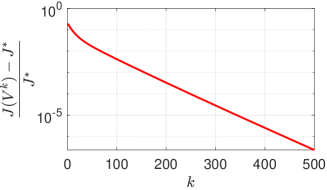
Figure 3: Convergence of DeePO for the LQR with offline data, where $J^{*}$ is obtained by solving the convex program of the LQR problem with covariance parameterization (17).

Fig. 3 shows that the LQR cost converges to $J^{*}$ at a linear rate, which implies that the sublinear rate in Theorem 1 may be conservative.

VI-B Convergence of DeePO for the adaptive learning of the LQR with online closed-loop data

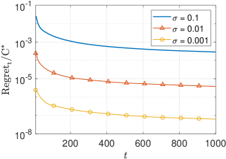
Figure 4: Convergence of DeePO for adaptive learning of the LQR under different level of noise $\sigma$.

In this subsection, we perform Algorithm 1 for the adaptive learning of the LQR with online closed-loop data to validate Theorem 2. We set $x_{0}=0$ and $u_{t}\sim\mathcal{N}(0,I_{2})$ for $t<t_{0}$ with $t_{0}=8$. For $t\geq t_{0}$, we set $u_{t}=K_{t}x_{t}+v_{t}$ with $v_{t}\sim\mathcal{N}(0,I_{2})$ to ensure persistency of excitation. The white noise sequence $\{w_{t}\}$ is drawn from a uniform distribution, where each element of $w_{t}$ is uniformly sampled from $[0,\sigma]$. We consider three noise levels $\sigma\in\{0.1,0.01,0.001\}$, which correspond approximately to the SNR $\in[0,5],[10,15],[20,25]$ dB, respectively. We set the stepsize to $\eta=0.01$.

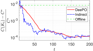
Figure 5: Comparison of DeePO and indirect methods for adaptive learning of the LQR. We also plot the performance gap of the initial gain (dashed green line) computed by single batch methods from offline data [11, 12, 13].

Fig. 4 shows that average regret matches the expected sublinear decrease $\mathcal{O}(1/\sqrt{T})$ in Theorem 2. Moreover, since the bounded noise $w_{t}$ has non-zero mean, the regret does not converge to zero. Roughly, the bias scales as SNR^-2 rather than the expected SNR^-1/2, which implies that our bound on the bias term in Theorem 2 may be conservative. Bridging this gap requires tighter perturbation bounds.

VI-C Comparison with indirect certainty-equivalence control for adaptive learning of the LQR

Consider the system proposed in [3, Section 6]

$$A=\begin{bmatrix}1.01&0.01&0\\ 0.01&1.01&0.01\\ 0&0.01&1.01\end{bmatrix},~{}B=I_{3},$$ (35)

which corresponds to a discrete-time marginally unstable Laplacian system. Let $Q=R=I_{3}$. To verify that our method can handle unbounded noise, let $w_{t}\sim\mathcal{N}(0,I_{3}/100)$ which corresponds to SNR $\in[0,5]$. We compare Algorithm 1 with the indirect adaptive approach in [7, 8]. Specifically, the indirect methods alternate between finding the certainty-equivalence LQR gain $K_{t}$ (8) and using $u_{t}=K_{t}x_{t}+v_{t}$ with $v_{t}\sim\mathcal{N}(0,I_{2})$ to obtain the new state $x_{t+1}$. For both methods, we use the solution to the LQR problem with covariance parameterization (17) based on $(X_{0,t_{0}},U_{0,t_{0}},X_{1,t_{0}})$ as the initial stabilizing gain $K_{t_{0}}$.

Fig. 5 shows that the performance gap of both methods converges at a sublinear rate to $10^{-4}$ in $200$ time steps. By using online closed-loop data, both methods improve the performance over the initial gain, which equals the solution to the regularized LQR parameterization (18) based on offline data $(X_{0,t_{0}},U_{0,t_{0}},X_{1,t_{0}})$ [11, 12, 13] (see Remark 2). For $t\leq 20$, the indirect approach exhibits faster convergence than DeePO. This is because DeePO only performs one-step projected gradient descent per time, and hence requires more iterations to asymptotically approach the performance of the certainty-equivalence LQR. Indeed, they achieve similar performance for $t\geq 60$. Moreover, thanks to the recursive policy update, the curve of DeePO is significantly smoother.

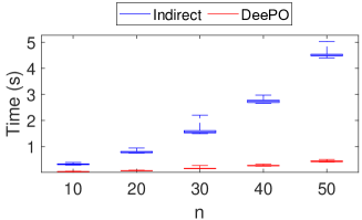
Figure 6: Comparison of the computation time for performing $100$ time steps.

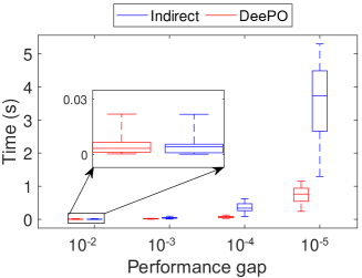
Figure 7: Comparison of the computation time to achieve a specified performance gap.

Next, we compare their efficiency in terms of real-time computation. For a fair comparison, we apply rank-one update for both Algorithm 1 (see Section V-B) and SysID (7) in indirect methods. With identified model, the certainty-equivalence LQR problem (8) is solved using the dlqr function in MATLAB. First, we evaluate the computation time for systems with different dimensions during $100$ time steps. Let $n=m\in\{10,20,30,40,50\}$. For each instance, we perform $50$ independent trials, where each trial uses randomly generated stable state matrix $A$ and identity input matrix $B$. The box plot in Fig. 6 shows that DeePO is significantly more efficient than indirect methods, and their gap scales significantly with $n$. Second, we also compare the computation time to achieve different performance gap $\epsilon:={(C(K)-C^{*})}/C^{*}$ for a fixed system dimension $n=4$. Fig. 7 shows the results from $50$ independent trials. For a large performance gap (e.g., $\epsilon=10^{-2}$), the computation time is similar for both methods. This reveals that while the indirect method converges faster at the beginning (see Fig. 5), its real-time computation is more time-consuming. For a small performance gap (e.g., $\epsilon=10^{-5}$), DeePO requires significantly less computation time. Since a rank-one update has been applied in both methods, the difference of computational efficiency is due to DeePO only performing one-step gradient descent per time, but the indirect method needs to solve a Riccati equation.

VI-D Comparison with zeroth-order PO

	$\epsilon=1$	$\epsilon=0.1$	$\epsilon=0.01$
Zeroth-order PO (# of trajectories)	$1414$	$43850$	$142865$
DeePO (# of input-state pairs)	$10$	$24$	$48$

TABLE I: Comparison of the sample complexity to achieve a specified performance gap $\epsilon$.

While the zeroth-order PO methods[27, 29, 28] are episodic (see Fig. 1), we compare them with DeePO in Algorithm 1 to demonstrate our sample efficiency. We use the simulation model (35) with $Q=R=I_{3}$ and $w_{t}\sim\mathcal{N}(0,0.01I_{n})$. We adopt the zeroth-order PO method in (11)-(12) for comparison. In particular, we use a minibatch of $30$ zeroth-order samples for (12) to reduce the variance of gradient estimate. We set the smooth radius to $r=0.02$, the stepsize to $\eta=10^{-3}$, and the length of the trajectory to $T=50$. The setting for Algorithm 1 is the same as in Section VI-B. For both methods, we use $-0.15\times I_{3}$ as the initial stabilizing gain.

Table I demonstrates the sample complexity of zeroth-order PO (in terms of number of trajectories) and DeePO (in terms of number of input-state pairs) to achieve different performance gap. It indicates that the zeroth-order PO is vastly less efficient for solving the LQR problem, which is in line with the sample complexity discussion in [43].

VII Concluding remarks

In this paper, we have proposed the DeePO method for the adaptive learning of the LQR based on a covariance parameterization. Hence, we have addressed the open problem in [16, 14, 22]. We have shown that under a quantitative condition of PE inputs and the boundedness of noises, the average regret is governed by two terms signifying a sublinear decrease in time plus a bias scaling inversely with the SNR. We have validated our theoretical findings and shown the superior computational and sample efficiency via simulations.

We believe that our paper leads to fruitful future works. By using the covariance parameterization, we can solve other classical control problems (e.g., the $\mathcal{H}_{\infty}$ problem considered in [10]) in a direct data-driven fashion and investigate the performance of DeePO on them. It would be desirable to understand whether regularization methods can be used to promote robustness of DeePO under our covariance parameterization (17), which has been achieved for the existing LQR parameterization (10) in [33]. As discussed in Section V-D, it would be valuable to study DeePO in the stochastic noise setting and extend to time-varying systems. As observed in the simulation, the sublinear rate in Theorem 1 and the dependence on the SNR in Theorem 2 may be conservative, and their sharper analysis is an important future work.

Appendix A Proof of Lemma 1

By the covariance parameterization (14) and the positive definiteness of $\Lambda$ (due to the PE condition (6)), $V$ is uniquely determined as $V=\Lambda^{-1}[K^{\top},I_{n}]^{\top}$. Then, the LQR problem with covariance parameterization (17) can be reformulated as

$$\mathop{\text{minimize}}\limits_{K,\Sigma\geq 0}~{}\text{Tr}\left((Q+K^{\top}RK)\Sigma\right),$$

$$\text{subject to}~{}~{}\Sigma=I_{n}+X_{1}D_{0}^{\dagger}\begin{bmatrix}K\\ I_{n}\end{bmatrix}\Sigma\begin{bmatrix}K\\ I_{n}\end{bmatrix}^{\top}(X_{1}D_{0}^{\dagger})^{\top}.$$

By the definition $[\hat{B},\hat{A}]=X_{1}D_{0}^{\dagger}$ in (7), this problem is exactly the certainty-equivalence LQR problem (8).

Appendix B Proof in Section IV

We provide some useful bounds which will be invoked frequently in the rest of the paper.

Lemma 11

For $V\in\mathcal{S}$, it holds that (i) $\|\Sigma_{V}\|\leq\text{Tr}(\Sigma_{V})\leq{J(V)}/{\underline{\sigma}(Q)},$ (ii) $\|P_{V}\|\leq J(V),$ and (iii) $\|\overline{U}_{0}V\|_{F}\leq({J(V)}/{\underline{\sigma}(R)})^{{1}/{2}}.$

Proof:

The proof of (i) and (ii) follows directly from the definition of $J(V)$. To show (iii), we have $J(V)=\text{Tr}((Q+V^{\top}\overline{U}_{0}^{\top}R\overline{U}_{0}V)\Sigma_{V})\geq\text{Tr}(V^{\top}\overline{U}_{0}^{\top}R\overline{U}_{0}V\Sigma_{V})\geq\text{Tr}(V^{\top}\overline{U}_{0}^{\top}\overline{U}_{0}V)\underline{\sigma}(R)=\|\overline{U}_{0}V\|_{F}^{2}\underline{\sigma}(R).$  

B-A Proof of Lemma 2

The proof follows the same vein as that of [26, Proposition 1]. We first compute the differential of $P_{V}$. Define $E_{V}:=(\overline{U}_{0}^{\top}R\overline{U}_{0}+\overline{X}_{1}^{\top}P_{V}\overline{X}_{1})V$. By definition, it holds that

$$dP_{V}=dV^{\top}E_{V}+E^{\top}_{V}dV+V^{\top}\overline{X}_{1}^{\top}dP_{V}\overline{X}_{1}V.$$

Since $\rho(\overline{X}_{1}V)<1$, we obtain

$$dP_{V} =\sum_{i=0}^{\infty}\left(V^{\top}\overline{X}_{1}^{\top}\right)^{i}\left(dV^{\top}E_{V}+E^{\top}_{V}dV\right)\left(\overline{X}_{1}V\right)^{i}$$

$$\text{Tr}(dP_{V}) =\text{Tr}\left(2\sum_{i=0}^{\infty}(\overline{X}_{1}V)^{i}(V^{\top}\overline{X}_{1}^{\top})^{i}\cdot E^{\top}_{V}dV\right)$$

$$=\text{Tr}\left(2\Sigma_{V}E_{V}^{\top}dV\right).$$

B-B Proof of Lemma 3

We apply [40, Theorem 1] to prove Lemma 3. We first relate the LQR problem with covariance parameterization (17) to the following convex reparameterization via a change of variables $V=L\Sigma^{-1}$:

$$\mathop{\text{minimize}}\limits_{L,\Sigma}~{}f(L,\Sigma):=\text{Tr}(Q\Sigma)+\text{Tr}(L\Sigma^{-1}L^{\top}\overline{U}_{0}^{\top}R\overline{U}_{0}),$$ (36)

$$\text{subject to}~{}~{}\Sigma=\overline{X}_{0}L,~{}\begin{bmatrix}\Sigma-I_{n}&\overline{X}_{1}L\\ L^{\top}\overline{X}_{1}^{\top}&\Sigma\end{bmatrix}\succeq 0.$$

Let $\mathcal{L}$ denote the feasible set of (36). The equivalence between (17) and (36) are established below.

Lemma 12

For any $(L,\Sigma)\in\mathcal{L}$, it holds that $\Sigma$ is invertible and $L\Sigma^{-1}\in\mathcal{S}$. Moreover, for $V\in\mathcal{S}$, we have

$$J(V)=\min_{L,\Sigma}\{f(L,\Sigma),\text{s.t.}(L,\Sigma)\in\mathcal{L},L\Sigma^{-1}=V\}.$$ (37)

Proof:

Applying the Schur complement to the linear matrix inequality constraint in (36) yields $\Sigma\succ 0$ and

$$\Sigma-I_{n}-\overline{X}_{1}L\Sigma^{-1}L^{\top}\overline{X}_{1}^{\top}\succeq 0.$$

By the non-singularity of $\Sigma$, let $V=L\Sigma^{-1}$. Then, a substitution of $L=V\Sigma$ into the above inequality yields

$$\Sigma-I_{n}-\overline{X}_{1}V\Sigma V^{\top}\overline{X}_{1}^{\top}\succeq 0.$$

Thus, $\overline{X}_{1}V$ is stable, i.e., $\rho(\overline{X}_{1}V)<1$. Since the first constraint of (36) implies $\overline{X}_{0}V=\overline{X}_{0}L\Sigma^{-1}=\Sigma\Sigma^{-1}=I_{n}$, it holds that $V=L\Sigma^{-1}\in\mathcal{S}$.

Next, we prove the second statement. Using the constraint $V=L\Sigma^{-1}$ and the Schur complement, the right-hand side of (37) becomes

$$\min_{\Sigma\succ 0}~{}\text{Tr}\left(\left(Q+V^{\top}\overline{U}_{0}^{\top}R\overline{U}_{0}V\right)\Sigma\right)$$ (38)

$$~{}\text{s.t.}~{}\overline{X}_{0}V=I_{n},\Sigma\succeq I_{n}+\overline{X}_{1}V\Sigma V^{\top}\overline{X}_{1}^{\top}.$$

Let $\Sigma(\Theta)$ be the unique positive definite solution of the Lyapunov equation

$$\Sigma(\Theta)=\Theta+\overline{X}_{1}V\Sigma(\Theta)V^{\top}\overline{X}_{1}^{\top}$$

with $\Theta\succeq I_{n}$. By monotonicity of $\Sigma(\Theta)$, we have $\Sigma(\Theta)\succeq\Sigma(I_{n})$. Since $Q+V^{\top}\overline{U}_{0}^{\top}R\overline{U}_{0}V\succ 0$, the minimum of (38) is attained at $\Sigma(I_{n})$, which is $\text{Tr}((Q+V^{\top}\overline{U}_{0}^{\top}R\overline{U}_{0}V)\Sigma(I_{n}))$ with $\overline{X}_{0}V=I_{n}$. This is exactly the definition of $J(V)$.  

Next, we show the convexity of the reparameterization (36).

Lemma 13

The feasible set $\mathcal{L}$ is convex, and $f(L,\Sigma)$ is convex over $\mathcal{L}$. Moreover, $f(L,\Sigma)$ is differentiable over an open domain that contains $\mathcal{L}$.

Proof:

Since the constraints in (36) are linear in $(L,\Sigma)$, the feasible set $\mathcal{L}$ is convex. Clearly, $f(L,\Sigma)$ is differential over $\mathcal{L}$. Hence, $f$ is convex over $\mathcal{L}$. Define the derivative and Hessian of $f$ along the direction $(\tilde{L},\tilde{\Sigma})$ as

$$f^{\prime}(L,\Sigma)[(\tilde{L},\tilde{\Sigma})]:=\frac{d}{d\tau}f(L+\tau\tilde{L},\Sigma+\tau\tilde{\Sigma})\big{|}_{\tau=0},$$

$$\nabla^{2}f(L,\Sigma)[(\tilde{L},\tilde{\Sigma}),(\tilde{L},\tilde{\Sigma})]:=\frac{d^{2}}{d\tau^{2}}f(L+\tau\tilde{L},\Sigma+\tau\tilde{\Sigma})\big{|}_{\tau=0},$$

respectively. By the definition of $f(L,\Sigma)$, it holds that

$$f^{\prime}(L,\Sigma)[(\tilde{L},\tilde{\Sigma})]= \text{Tr}(Q\tilde{\Sigma})-\text{Tr}(\Sigma^{-1}L^{\top}\overline{U}_{0}^{\top}R\overline{U}_{0}L\Sigma^{-1}\tilde{\Sigma})$$

$$+2\text{Tr}(\tilde{L}\Sigma^{-1}L^{\top}\overline{U}_{0}^{\top}R\overline{U}_{0}).$$

For brevity, let $\overline{R}=\overline{U}_{0}^{\top}R\overline{U}_{0}$. Then, the Hessian satisfies

$$\nabla^{2}f(L,\Sigma)[(\tilde{L},\tilde{\Sigma}),(\tilde{L},\tilde{\Sigma})]$$

$$=\text{Tr}(\Sigma^{-1}\tilde{\Sigma}\Sigma^{-1}L^{\top}\overline{R}L\Sigma^{-1}\tilde{\Sigma})+\text{Tr}(\Sigma^{-1}L^{\top}\overline{R}L\Sigma^{-1}\tilde{\Sigma}\Sigma^{-1}\tilde{\Sigma})$$

$$~{}~{}~{}+2\text{Tr}(\tilde{L}\Sigma^{-1}\tilde{L}^{\top}\overline{R})-4\text{Tr}(\overline{R}L\Sigma^{-1}\tilde{\Sigma}\Sigma^{-1}\tilde{L}^{\top})$$

$$=2\left\|R^{\frac{1}{2}}(\overline{U}_{0}\tilde{L}-\overline{U}_{0}L\Sigma^{-1}\tilde{\Sigma})\Sigma^{-\frac{1}{2}}\right\|_{F}^{2}\geq 0,$$

which completes the proof.  

By Lemmas 12 and 13, the LQR problem with covariance parameterization (17) and its convex reparameterization (36) satisfy the assumptions of [40, Theorem 1]. Then, there exists $c>0$ and a direction $Z\in\mathcal{N}(\overline{X}_{0})$ with $\|Z\|_{F}=1$ in the descent cone of $\mathcal{S}(a)$ such that

$$J^{\prime}(V)[Z]\leq-c(J(V)-J^{*}),$$

where $J^{\prime}(V)[Z]$ denotes the derivative of $J(V)$ along the direction $Z$. Let $Z^{\prime}=\Pi_{\overline{X}_{0}}\nabla J(V)/\|\Pi_{\overline{X}_{0}}\nabla J(V)\|_{F}$ be the normalized projected gradient. Since both $Z$ and $Z^{\prime}$ are feasible directions but $Z^{\prime}$ is the direction of the projected gradient, we have $J^{\prime}(V)[Z^{\prime}]\leq J^{\prime}(V)[Z],\forall Z\in\mathcal{N}(\overline{X}_{0})$. Thus, it holds that $J(V)-J^{*}\leq\|\Pi_{\overline{X}_{0}}\nabla J(V)\|/c$.

Next, we derive an explicit upper bound of $1/c$ over $V\in\mathcal{S}(a)$. By [40, Theorem 1], $c$ is given by

$$c=(2\max\{\|L-L^{*}\|_{F}/\underline{\sigma}(\Sigma),\|\Sigma-\Sigma^{*}\|_{F}\|L\|/\underline{\sigma}^{2}(\Sigma)\})^{-1},$$

where $(L^{*},\Sigma^{*})$ is an optimal solution of (36), and

$$(L,\Sigma)=\mathop{\text{argmin}}\limits_{(L^{\prime},\Sigma^{\prime})\in\mathcal{L}}\{f(L^{\prime},\Sigma^{\prime}),\text{s.t.}~{}L^{\prime}(\Sigma^{\prime})^{-1}=V\}.$$

We now provide upper bounds for $\underline{\sigma}^{-1}(\Sigma),\|\Sigma\|_{F},\|L\|_{F}$. Since $\underline{\sigma}(\Sigma)\geq 1$, it holds $\underline{\sigma}^{-1}(\Sigma)\leq 1$. The sublevel set gives $\text{Tr}(Q\Sigma)\leq a$, and hence $\|\Sigma\|_{F}\leq a/\underline{\sigma}(Q)$. Since

$$\underline{\sigma}(R)\underline{\sigma}^{2}(\overline{U}_{0})\|\Sigma\|^{-1}\|L\|^{2}_{F}\leq\text{Tr}\left(L\Sigma^{-1}L^{\top}\overline{U}_{0}^{\top}R\overline{U}_{0}\right)$$

$$\leq\text{Tr}(Q\Sigma)+\text{Tr}\left(L\Sigma^{-1}L^{\top}\overline{U}_{0}^{\top}R\overline{U}_{0}\right)\leq a,$$

an upper bound of $\|L\|_{F}$ is given by

$$\|L\|_{F}\leq\left(\frac{a\|\Sigma\|}{\underline{\sigma}(R)\underline{\sigma}^{2}(\overline{U}_{0})}\right)^{{1}/{2}}\leq\frac{a}{(\underline{\sigma}(Q)\underline{\sigma}(R))^{1/2}\underline{\sigma}(\overline{U}_{0})}.$$

Those bounds are also true for $(L^{*},\Sigma^{*})$. Furthermore, we can provide the following upper bound

$$\frac{1}{c}\leq\frac{4a}{(\underline{\sigma}(Q)\underline{\sigma}(R))^{1/2}\underline{\sigma}(\overline{U}_{0})}\max\left\{1,\frac{a}{\underline{\sigma}(Q)}\right\}.$$

Since $\mathcal{S}(a)$ is non-empty, we have $a\geq J^{*}\geq\underline{\sigma}(Q)$. Hence,

$$\frac{1}{c}\leq\frac{4a^{2}}{(\underline{\sigma}(Q))^{{3}/{2}}(\underline{\sigma}(R))^{{1}/{2}}\underline{\sigma}(\overline{U}_{0})}:=\mu(a).$$

B-C Proof of Lemma 4

We show the local smoothness of $J(V)$ by providing an upper bound for $\|\nabla^{2}J(V)\|:=\sup_{\|Z\|_{F}=1}\left|\nabla^{2}J(V)[Z,Z]\right|$ over the sublevel set $V\in\mathcal{S}(a)$. We first present a formula for the Hessian of $J(V)$.

Lemma 14

For $V\in\mathcal{S}$ and a feasible direction $Z\in\mathbb{R}^{(n+m)\times n}$, the Hessian of $J(V)$ is characterized as

$$\nabla^{2}J(V)[Z,Z]=4\text{Tr}\left(Z^{\top}\overline{X}_{1}^{\top}P^{\prime}[Z]\overline{X}_{1}V\Sigma_{V}\right)$$

$$+2\text{Tr}\left(Z^{\top}\left(\overline{U}_{0}^{\top}R\overline{U}_{0}+\overline{X}_{1}^{\top}P_{V}\overline{X}_{1}\right)Z\Sigma_{V}\right),$$

where $P^{\prime}[Z]=\sum_{i=0}^{\infty}(V^{\top}\overline{X}_{1}^{\top})^{i}(Z^{\top}E_{V}+E_{V}^{\top}Z)(\overline{X}_{1}V)^{i}.$

Proof:

By the definition of $P_{V}$ in (20), it holds that

$$P^{\prime}[Z] =Z^{\top}\overline{X}_{1}^{\top}P_{V}\overline{X}_{1}V+V^{\top}\overline{X}_{1}^{\top}P_{V}\overline{X}_{1}Z$$

$$+Z^{\top}\overline{U}_{0}^{\top}R\overline{U}_{0}V+V^{\top}\overline{U}_{0}^{\top}R\overline{U}_{0}Z+V^{\top}\overline{X}_{1}^{\top}P^{\prime}[Z]\overline{X}_{1}V$$

$$=Z^{\top}E_{V}+E_{V}^{\top}Z+V^{\top}\overline{X}_{1}^{\top}P^{\prime}[Z]\overline{X}_{1}V.$$

Then, we have $E^{\prime}[Z]=(\overline{U}_{0}^{\top}R\overline{U}_{0}+\overline{X}_{1}^{\top}P_{V}\overline{X}_{1})Z+\overline{X}_{1}^{\top}P^{\prime}[Z]\overline{X}_{1}V,$ and the Hessian $P^{\prime\prime}[Z]$ satisfies

$$P^{\prime\prime}[Z] =V^{\top}\overline{X}_{1}^{\top}P^{\prime}[Z]\overline{X}_{1}Z+Z^{\top}\overline{X}_{1}^{\top}P^{\prime}[Z]\overline{X}_{1}V$$

$$~{}~{}~{}+Z^{\top}E^{\prime}[Z]+(E^{\prime}[Z])^{\top}Z+V^{\top}\overline{X}_{1}^{\top}P^{\prime\prime}[Z]\overline{X}_{1}V$$

$$=S+V^{\top}\overline{X}_{1}^{\top}P^{\prime\prime}[Z]\overline{X}_{1}V,$$

where $S=2V^{\top}\overline{X}_{1}^{\top}P^{\prime}[Z]\overline{X}_{1}Z+2Z^{\top}\overline{X}_{1}^{\top}P^{\prime}[Z]\overline{X}_{1}V+2Z^{\top}(\overline{U}_{0}^{\top}R\overline{U}_{0}+\overline{X}_{1}^{\top}P_{V}\overline{X}_{1})Z.$

By the definition of $J(V)$ in (19), it holds that $\nabla^{2}J(V)[Z,Z]=\text{Tr}(P^{\prime\prime}[Z])=\text{Tr}\left(S\Sigma_{V}\right).$  

Next, we provide an upper bound for $\|\nabla^{2}J(V)\|$. Let $Z\in\mathbb{R}^{(n+m)\times n}$ be a feasible direction with $\|Z\|_{F}=1$. Then,

$$\|\nabla^{2}J(V)\|\leq 4\left|\text{Tr}\left(Z^{\top}\overline{X}_{1}^{\top}P^{\prime}[Z]\overline{X}_{1}V\Sigma_{V}\right)\right|$$ (39)

$$+2\left\|Z^{\top}\left(\overline{U}_{0}^{\top}R\overline{U}_{0}+\overline{X}_{1}^{\top}P_{V}\overline{X}_{1}\right)Z\right\|\text{Tr}(\Sigma_{V}).$$

For the first term, we have that

$$\left|\text{Tr}(Z^{\top}\overline{X}_{1}^{\top}P^{\prime}[Z]\overline{X}_{1}V\Sigma_{V})\right|$$

$$\leq\left\|Z^{\top}\overline{X}_{1}^{\top}P^{\prime}[Z]\overline{X}_{1}V\Sigma_{V}^{\frac{1}{2}}\right\|_{F}\left\|\Sigma_{V}^{\frac{1}{2}}\right\|_{F}$$

$$\leq\left\|\overline{X}_{1}\right\|_{F}^{2}\left\|\overline{X}_{1}V\Sigma_{V}^{\frac{1}{2}}\right\|_{F}\left\|\Sigma_{V}^{\frac{1}{2}}\right\|_{F}\left\|P^{\prime}[Z]\right\|_{F}$$

$$\leq\left\|\overline{X}_{1}\right\|_{F}^{2}\|P^{\prime}[Z]\|_{F}\cdot a/{\underline{\sigma}(Q)},$$

where the last inequality follows from Lemma 11 and

$$\left\|\overline{X}_{1}V\Sigma_{V}^{\frac{1}{2}}\right\|_{F}^{2}=\text{Tr}\left(\overline{X}_{1}V\Sigma_{V}V^{\top}\overline{X}_{1}^{\top}\right)$$

$$\leq\text{Tr}\left(\overline{X}_{1}V\Sigma_{V}V^{\top}\overline{X}_{1}^{\top}+I_{n}\right)=\left\|\Sigma_{V}^{\frac{1}{2}}\right\|_{F}^{2}.$$

Thus, we only need to provide an upper bound for $\|P^{\prime}[Z]\|_{F}$. Since $\|Z\|_{F}=1$ and

$$Z^{\top}E_{V}+E_{V}^{\top}Z \preceq Z^{\top}\left(\overline{U}_{0}^{\top}R\overline{U}_{0}+\overline{X}_{1}^{\top}P_{V}\overline{X}_{1}\right)Z$$

$$~{}~{}~{}+V^{\top}\left(\overline{U}_{0}^{\top}R\overline{U}_{0}+\overline{X}_{1}^{\top}P_{V}\overline{X}_{1}\right)V$$

$$=Z^{\top}\left(\overline{U}_{0}^{\top}R\overline{U}_{0}+\overline{X}_{1}^{\top}P_{V}\overline{X}_{1}\right)Z+P_{V}-Q$$

$$\preceq\left(\left(\xi(a)+a\right)/{\underline{\sigma}(Q)}-1\right)Q,$$

it follows from the definition that

$$P^{\prime}[Z] =\sum_{i=0}^{\infty}\left(V^{\top}\overline{X}_{1}^{\top}\right)^{i}\left(Z^{\top}E_{V}+E_{V}^{\top}Z\right)(\overline{X}_{1}V)^{i}$$

$$\preceq\left(\left(\xi(a)+a\right)/{\underline{\sigma}(Q)}-1\right)P_{V}.$$

Then, it holds that $\|P^{\prime}[Z]\|_{F}\leq a\left(\left(\xi(a)+a\right)/{\underline{\sigma}(Q)}-1\right)$, and the first term of the right-hand side of (39) is bounded by $4\left(\left(\xi(a)+a\right)/{\underline{\sigma}(Q)}-1\right)\|\overline{X}_{1}\|_{F}^{2}{a^{2}}/{\underline{\sigma}(Q)}$. By Lemma 11, the second term is bounded by $2\xi(a){a}/{\underline{\sigma}(Q)}$. That is,

$$\|\nabla^{2}J(V)\|\leq 4a^{2}\left(\xi(a)+a-\underline{\sigma}(Q)\right)\frac{\|\overline{X}_{1}\|_{F}^{2}}{\underline{\sigma}^{2}(Q)}+\frac{2\xi(a)a}{\underline{\sigma}(Q)}.$$

In conjunction with the Taylor expansion of $J(V)$, the proof is completed.

B-D Proof of Theorem 1

Define $V_{\eta}:=V-\eta\Pi_{\overline{X}_{0}}\nabla J(V)$. We first show that for a non-optimal $V\in\mathcal{S}(a)$ and any $\eta\in[0,1/l(a)]$, it holds $V_{\eta}\in\mathcal{S}(a)$.

Define $\mathcal{S}^{o}(a):=\{V\in\mathcal{S}\mid J(V)<a\}$, and $(\mathcal{S}^{o}(a))^{c}$ as its complement, which is closed. By Lemma 4, given $\phi\in(0,1)$, there exists $b>0$ such that $\|\nabla^{2}J(V)\|\leq(1+\phi)l(a)$ for $V\in\mathcal{S}(a+b)$. Clearly, $\mathcal{S}(a)\cap(\mathcal{S}^{o}(a+b))^{c}=\emptyset$. Then, the distance between them $d:=\inf\{\|V^{\prime}-V\|,\forall V\in\mathcal{S}(a),V^{\prime}\in(\mathcal{S}^{o}(a+b))^{c}\}$ is positive. Let $\overline{N}\in\mathbb{N}_{+}$ be large enough such that $2/(\overline{N}(1+\phi)l(a))<d/\|\Pi_{\overline{X}_{0}}\nabla J(V)\|$, which is well-defined since $V$ is not optimal. Define a stepsize $\tau\in[0,2/(\overline{N}(1+\phi)l(a))]$. Since $\tau<d/\|\Pi_{\overline{X}_{0}}\nabla J(V)\|$, we have $\|V_{\tau}-V\|<d$, i.e., $V_{\tau}\in\mathcal{S}(a+b)$. Thus, we can apply Lemma 4 over $\mathcal{S}(a+b)$ to show $J(V_{\tau})-J(V)\leq-\tau(1-{(1+\phi)l(a)\tau}/{2})\|\Pi_{\overline{X}_{0}}\nabla J(V)\|^{2}\leq 0,$ where the last inequality follows from $\tau\leq 2/(1+\phi)l(a)$. This implies that the segment between $V$ and $V_{\tau}$ is contained in $\mathcal{S}(a)$. It is also clear that $V_{2\tau}\in\mathcal{S}(a+b)$ since $\|V_{2\tau}-V_{\tau}\|<d$. Then, we can use induction to show that the segment between $V$ and $V_{N\tau}$ for $N\in\mathbb{N}_{+}$ is in $\mathcal{S}(a)$ as long as $N\tau\leq 2/(1+\phi)l(a)$. Since $\phi\in(0,1)$, we let $\eta\leq 1/l(a)$ to ensure the segment between $V$ and $V_{\eta}$ contained in $\mathcal{S}(a)$.

Then, a simple induction leads to that for $\eta\in[0,1/l^{0}]$, the update (21) satisfies $V^{k}\in\mathcal{S}(J(V^{0})),\forall k\in\mathbb{N}$. Moreover, the cost satisfies

$$J(V^{k+1})\leq J(V^{k})-\eta\left(1-\frac{l^{0}\eta}{2}\right)\|\Pi_{\overline{X}_{0}}\nabla J(V^{k})\|^{2}.$$

Using Lemma 3 and subtracting $J^{*}$ in both sides yield

$$J(V^{k+1})-J^{*}\leq J(V^{k})-J^{*}-\frac{2\eta-l^{0}\eta^{2}}{2(\mu^{0})^{2}}(J(V^{k})-J^{*})^{2}.$$

Dividing by $(J(V^{k})-J^{*})(J(V^{k+1})-J^{*})$ in both sides and noting $J(V^{k+1})\leq J(V^{k})$ lead to

$$\frac{2\eta-l^{0}\eta^{2}}{2(\mu^{0})^{2}}\leq\frac{1}{J(V^{k+1})-J^{*}}-\frac{1}{J(V^{k})-J^{*}}.$$

Summing up both sides over $0,1,\dots,k-1$ and using telescopic cancellation yield that

$$\frac{k(2\eta-l^{0}\eta^{2})}{2(\mu^{0})^{2}}\leq\frac{1}{J(V^{k})-J^{*}}.$$

Letting the right-hand side of the above inequality equal $\epsilon$ and solving $k$ yields the required number of iterations (22).

Appendix C Proof in Section V

C-A Proof of Lemma 5

Since $\underline{\sigma}(\overline{U}_{0,t})\geq\underline{\sigma}(U_{0,t})\underline{\sigma}(D_{0,t})/t$, we provide lower bounds for $\underline{\sigma}(U_{0,t})$ and $\underline{\sigma}(D_{0,t})$, respectively.

Let $\theta_{l}\in\mathbb{R}^{m},\theta_{r}\in\mathbb{R}^{t}$ be the left and right singular vectors of $U_{0,t}$ corresponding to the minimal singular value $\underline{\sigma}(U_{0,t})$, respectively, i.e., $\theta_{l}^{\top}U_{0,t}=\underline{\sigma}(U_{0,t})\theta_{r}^{\top}$ with $\|\theta_{l}\|=\|\theta_{r}\|=1$. Define the diagonal block matrix $\Omega:=\text{diag}(\theta_{l}^{\top},\dots,\theta_{l}^{\top})\in\mathbb{R}^{n\times nm}$, which has full row rank. Then, it holds that $\Omega\cdot\mathcal{H}_{n+1}(U_{0,t})=\underline{\sigma}(U_{0,t})\mathcal{H}_{n+1}(\theta_{r})$, and hence

$$\underline{\sigma}(\Omega)\underline{\sigma}(\mathcal{H}_{n+1}(U_{0,t}))\leq\underline{\sigma}(U_{0,t})\|\mathcal{H}_{n+1}(\theta_{r})\|.$$ (40)

Since $\|\theta_{l}\|=\|\theta_{r}\|=1$, we have $\|\mathcal{H}_{n+1}(\theta_{r})\|\leq\sqrt{n+1}$ and $\underline{\sigma}(\Omega)=1$. Substituting them into (40) and using Assumption 2, we yield $\underline{\sigma}(U_{0,t})\geq\sqrt{t}\gamma/\zeta.$

By Assumption 2 and the robust fundamental lemma [41, Theorem 5], it follows that

$$\underline{\sigma}(D_{0,t})\geq\sqrt{t}\gamma-\frac{\omega\|\mathcal{H}_{n}(W_{0,t-1})\|}{\sqrt{n+1}}.$$

By Assumption 4, it holds that $\|\mathcal{H}_{n}(W_{0,t-1})\|\leq\|\mathcal{H}_{n}(W_{0,t-1})\|_{F}\leq\sqrt{n(t-n)}\delta\leq\sqrt{(n+1)t}\delta.$ Then, the hypothesis ${\delta}/{\gamma}\leq 1/(2\omega)$ leads to $\underline{\sigma}(D_{0,t})\geq\sqrt{t}\gamma/2$.

Hence, we have $\underline{\sigma}(\overline{U}_{0,t})\geq\underline{\sigma}(U_{0,t})\underline{\sigma}(D_{0,t})/t\geq\gamma^{2}/(2\zeta)$.

C-B Proof of Lemma 8

The proof leverages the following result on the perturbation theory for Lyapunov equations.

Lemma 15

Let $A\in\mathbb{R}^{n\times n}$ be stable and $\Sigma(A)=I_{n}+A\Sigma(A)A^{\top}$. If $\|A^{\prime}-A\|\leq 1/({4\|\Sigma(A)\|(1+\|A\|)}),$ then $A^{\prime}$ is stable and $\|\Sigma(A^{\prime})-\Sigma(A)\|\leq 4\|\Sigma(A)\|^{2}(1+\|A\|)\|A^{\prime}-A\|.$

Proof:

The proof follows the same vein as that of [27, Lemma 16] and is omitted for saving space.  

1) Proof of (31). By definition, the cost can be written as

$$J_{t}(V_{t}^{\prime})=\text{Tr}\left((Q+K_{t}^{\top}RK_{t})\Sigma_{t}(V_{t}^{\prime})\right)$$

$$C(K_{t})=\text{Tr}\left((Q+K_{t}^{\top}RK_{t})\Sigma_{K_{t}}\right)$$

with $\Sigma_{t}(V_{t}^{\prime})=I_{n}+\overline{X}_{1,t}V_{t}^{\prime}\Sigma_{t}(V_{t}^{\prime})(V_{t}^{\prime})^{\top}\overline{X}_{1,t}^{\top}$ and $\Sigma_{K_{t}}=I_{n}+(A+BK_{t})\Sigma_{K_{t}}(A+BK_{t})^{\top}$. Then, it holds that

$$|C(K_{t})-J_{t}(V_{t}^{\prime})| =|\text{Tr}(Q+K_{t}^{\top}RK_{t})(\Sigma_{K_{t}}-\Sigma_{t}({V_{t}^{\prime}}))|$$

$$\leq J_{t}(V_{t}^{\prime})\|\Sigma_{K_{t}}-\Sigma_{t}({V_{t}^{\prime}})\|.$$

Next, we provide an upper bound for $\|\Sigma_{K_{t}}-\Sigma_{t}({V_{t}^{\prime}})\|$ based on Lemma 15. Starting from (30), we have

$$\left\|A+BK_{t}-\overline{X}_{1,t}V_{t}^{\prime}\right\|\leq\frac{2\delta}{\gamma}\left(1+\sqrt{\frac{J_{t}(V_{t}^{\prime})}{\underline{\sigma}(R)}}\right)$$

$$\leq\frac{\underline{\sigma}^{2}(Q)}{4J_{t}(V_{t}^{\prime})(\underline{\sigma}(Q)+J_{t}(V_{t}^{\prime}))}\leq\frac{\underline{\sigma}(Q)}{4J_{t}(V_{t}^{\prime})(1+\|\overline{X}_{1,t}V_{t}^{\prime}\|)},$$

where the first inequality follows from Lemmas 5 and 11, the second from the condition on $\delta/\gamma$, and the last from $\|\overline{X}_{1,t}V_{t}^{\prime}\|\leq\|\overline{X}_{1,t}V_{t}^{\prime}\Sigma_{t}^{{1}/{2}}(V_{t}^{\prime})\|\|\Sigma_{t}^{{1}/{2}}(V_{t}^{\prime})\|\leq\|\Sigma_{t}(V_{t}^{\prime})\|\leq{J_{t}(V_{t}^{\prime})}/{\underline{\sigma}(Q)}.$

Then, it follows from Lemma 15 that

$$\left\|\Sigma_{K_{t}}-\Sigma_{t}(V_{t}^{\prime})\right\|\leq 4\left(\frac{J_{t}(V_{t}^{\prime})}{\underline{\sigma}(Q)}\right)^{2}\left(1+\|\overline{X}_{1,t}V_{t}^{\prime}\|\right)$$ (41)

$$\times\left\|A+BK_{t}-\overline{X}_{1,t}V_{t}^{\prime}\right\|.$$

Hence, the cost difference can be bounded as

$$\left|C(K_{t})-J_{t}(V_{t}^{\prime})\right|\leq J_{t}(V_{t}^{\prime})\|\Sigma_{K_{t}}-\Sigma_{t}({V_{t}^{\prime}})\|$$

$$\leq\left(\frac{4J_{t}^{3}(V_{t}^{\prime})}{\underline{\sigma}^{2}(Q)}\right)\left(1+\|\overline{X}_{1,t}V_{t}^{\prime}\|\right)\left\|A+BK_{t}-\overline{X}_{1,t}V_{t}^{\prime}\right\|$$

$$\leq{p(J_{t}(V_{t}^{\prime}))\delta}/{(2\gamma)}.$$

2) Proof of (32). By definition, we have

$$J_{t+1}(V_{t+1})=\text{Tr}\left((Q+K_{t}^{\top}RK_{t})\Sigma_{t+1}({V_{t+1}})\right)$$

with $\Sigma_{t+1}({V_{t+1}})=I_{n}+\overline{X}_{1,t+1}V_{t+1}\Sigma_{t+1}({V_{t+1}})V_{t+1}^{\top}\overline{X}_{1,t+1}^{\top}$. Then, it follows that $|J_{t+1}(V_{t+1})-J_{t}(V_{t}^{\prime})|=|\text{Tr}((Q+K_{t}^{\top}RK_{t})\left(\Sigma_{t+1}({V_{t+1}})-\Sigma_{t}(V_{t}^{\prime})\right))|\leq J_{t}(V_{t}^{\prime})\cdot\|\Sigma_{t+1}({V_{t+1}})-\Sigma_{t}(V_{t}^{\prime})\|.$ Since

$$\left\|\overline{X}_{1,t+1}V_{t+1}-\overline{X}_{1,t}V_{t}^{\prime}\right\|$$ (42)

$$=\left\|\overline{W}_{0,t+1}V_{t+1}-\overline{W}_{0,t}V_{t}^{\prime}\right\|$$

$$=\left\|{W}_{0,t+1}D_{0,t+1}^{\dagger}\begin{bmatrix}K_{t}\\ I_{n}\end{bmatrix}-{W}_{0,t}D_{0,t}^{\dagger}\begin{bmatrix}K_{t}\\ I_{n}\end{bmatrix}\right\|$$

$$\leq\left\|{W}_{0,t+1}D_{0,t+1}^{\dagger}-{W}_{0,t}D_{0,t}^{\dagger}\right\|(1+\|K_{t}\|)$$

$$\leq\frac{4\delta}{\gamma}\left(1+\sqrt{\frac{J_{t}(V_{t}^{\prime})}{\underline{\sigma}(R)}}\right)\leq\frac{\underline{\sigma}(Q)}{4J_{t}(V_{t}^{\prime})(1+\|\overline{X}_{1,t}V_{t}^{\prime}\|)},$$

it follows from Lemma 15 that

$$\left\|\Sigma_{t+1}({V_{t+1}})-\Sigma_{t}(V_{t}^{\prime})\right\|$$

$$\leq 4\left(\frac{J_{t}(V_{t}^{\prime})}{\underline{\sigma}(Q)}\right)^{2}\left(1+\|\overline{X}_{1,t}V_{t}^{\prime}\|\right)\left\|\overline{X}_{1,t+1}V_{t+1}-\overline{X}_{1,t}V_{t}^{\prime}\right\|$$

$$\leq\frac{16\delta}{\gamma}\left(\frac{J_{t}(V_{t}^{\prime})}{\underline{\sigma}(Q)}\right)^{2}\left(1+\frac{J_{t}(V_{t}^{\prime})}{\underline{\sigma}(Q)}\right)\left(1+\sqrt{\frac{J_{t}(V_{t}^{\prime})}{\underline{\sigma}(R)}}\right).$$

Then, the cost difference can be upper-bounded as

$$|J_{t+1}(V_{t+1})-J_{t}(V_{t}^{\prime})| \leq J_{t}(V_{t}^{\prime})\|\Sigma_{t+1}({V_{t+1}})-\Sigma_{t}(V_{t}^{\prime})\|$$

$$\leq p(J_{t}(V_{t}^{\prime}))\delta/\gamma.$$

3) Proof of (33). It follows by combining (31) and (32).

C-C Proof of Lemma 9

Let $P^{*}$ and $P_{t}^{*}$ be the solution to the algebraic Riccati equation of the ground-truth $(A,B)$ and the estimated system $(\hat{A}_{t},\hat{B}_{t})$, respectively, i.e.,

$$P^{*}=A^{\top}P^{*}A+Q-A^{\top}P^{*}B(R+B^{\top}P^{*}B)^{-1}B^{\top}P^{*}A,$$

$$P_{t}^{*}=\hat{A}_{t}^{\top}P_{t}^{*}\hat{A}_{t}+Q-\hat{A}_{t}^{\top}P_{t}^{*}\hat{B}_{t}(R+\hat{B}_{t}^{\top}P_{t}^{*}\hat{B}_{t})^{-1}\hat{B}_{t}^{\top}P_{t}^{*}\hat{A}_{t}.$$

By the perturbation theory for the discrete-time Riccati equation [4, Proposition 1], there exist two constants $\bar{c}_{1},\bar{c}_{2}$ depending only on $A,B,Q,R$, such that if $\|[\hat{B}_{t},\hat{A}_{t}]-[B,A]\|\leq\bar{c}_{1}$, then $\|P_{t}^{*}-P^{*}\|\leq\bar{c}_{2}\|[\hat{B}_{t},\hat{A}_{t}]-[B,A]\|.$ Since $\|[\hat{B}_{t},\hat{A}_{t}]-[B,A]\|=\|W_{0,t}D_{0,t}^{\dagger}\|\leq 2\delta/\gamma$, it suffices to let $\delta/\gamma\leq\bar{c}_{1}/2:=c_{1}$. Then, it follows that $\|P_{t}^{*}-P^{*}\|\leq\bar{c}_{2}\|[\hat{B}_{t},\hat{A}_{t}]-[B,A]\|\leq 2\bar{c}_{2}{\delta}/{\gamma}.$ Hence, it holds that $\left|C_{\text{CE},t}^{*}-C^{*}\right|=|\text{Tr}(P_{t}^{*})-\text{Tr}(P^{*})|\leq 2\sqrt{n}\bar{c}_{2}\delta/\gamma.$ By Lemma 1, it holds that $|C^{*}-J_{t}^{*}|=|C^{*}-C_{\text{CE},t}^{*}|$. Letting $c_{2}=2\sqrt{n}\bar{c}_{2}$ completes the proof.

C-D Proof of Lemma 10

The proof relies on the lower bounds of the gradient dominance and smoothness constants in Lemmas 6 and 7. For brevity, let $\mu_{t}:=\mu(J_{t}(V_{t}))$ and $\l_{t}:=l(J_{t}(V_{t}))$.

Lemma 16

For $V_{t}\in\mathcal{S}_{t}$, it holds that $l_{t}\geq c_{3}$ and $\mu_{t}\geq c_{4}$.

Proof:

By definition, it holds that $J_{t}(V_{t})\geq J_{t}^{*}\geq\underline{\sigma}(Q)$. Then, $l_{t}$ and $\mu_{t}$ can be lower-bounded accordingly.  

We use mathematical induction to show $J_{t}(V_{t})\leq\bar{J}$ for $t>t_{0}$. We first show that it holds at $t=t_{0}+1$. Since $J_{t_{0}}(V_{t_{0}}^{\prime})=J_{t_{0}}^{*}\leq\bar{J}$, the assumption of Lemma 8 is satisfied, and

$$J_{t_{0}+1}(V_{t_{0}+1})\leq J_{t_{0}}(V_{t_{0}}^{\prime})+{p(J_{t_{0}}(V_{t_{0}}^{\prime}))\delta}/{\gamma}\leq J_{t_{0}}^{*}+{\bar{p}\delta}/{\gamma}.$$

Using the condition $\delta/\gamma\leq{\eta}/{(2\bar{\mu}^{2}\bar{p})}$ and Lemma 16 lead to

$$J_{t_{0}+1}(V_{t_{0}+1})\leq J_{t_{0}}^{*}+\frac{\eta}{2\bar{\mu}^{2}}\leq J_{t_{0}}^{*}+\frac{1}{2\bar{l}\bar{\mu}^{2}}\leq J_{t_{0}}^{*}+\frac{1}{2c_{3}c_{4}^{2}}\leq\bar{J}.$$

Next, we assume that $J_{t}(V_{t})\leq\bar{J}$ and show $J_{t+1}(V_{t+1})\leq\bar{J}$. Since $J_{t}(V_{t})\leq\bar{J}$, we have $l_{t}\leq\bar{l}$ and $\eta\leq 1/\bar{l}\leq 1/l_{t}$. Following the same vein as the proof of Theorem 1, we can show that $V_{t}^{\prime}\in\mathcal{S}_{t}$ and

$$J_{t}(V_{t}^{\prime})-J_{t}(V_{t}) \leq-\eta\left(1-\frac{l_{t}\eta}{2}\right)\left\|\Pi_{\overline{X}_{0,t}}\nabla J_{t}(V_{t})\right\|^{2}$$ (43)

$$\leq-\frac{\eta}{2}\left\|\Pi_{\overline{X}_{0,t}}\nabla J_{t}(V_{t})\right\|^{2},$$

where the second inequality follows from $\eta\leq 1/l_{t}$. Hence, it holds that $J_{t}(V_{t}^{\prime})\leq J_{t}(V_{t})\leq\bar{J}$. By Lemma 8 and our condition $\delta/\gamma\leq{\eta}/{(2\bar{\mu}^{2}\bar{p})}$, we have

$$J_{t+1}(V_{t+1})-J_{t}(V_{t}^{\prime})\leq\frac{p(J_{t}(V_{t}^{\prime}))\delta}{\gamma}\leq\frac{\bar{p}\delta}{\gamma}\leq\frac{\eta}{2\bar{\mu}^{2}}.$$ (44)

Combing (43) and (44) and using Lemma 6 yield

$$J_{t+1}(V_{t+1})-J_{t}(V_{t}) \leq\frac{\eta}{2\bar{\mu}^{2}}-\frac{\eta}{2}\left\|\Pi_{\overline{X}_{0,t}}\nabla J_{t}(V_{t})\right\|^{2}$$ (45)

$$\leq\frac{\eta}{2\mu_{t}^{2}}-\frac{\eta}{2\mu^{2}_{t}}(J_{t}(V_{t})-J_{t}^{*})^{2}.$$

To show $J_{t+1}(V_{t+1})\leq\bar{J}$, we consider two cases. Suppose that $J_{t}(V_{t})\geq C^{*}+c_{1}c_{2}+1.$ By Lemma 9, it holds that $\left|C^{*}-J_{t}^{*}\right|\leq c_{2}\delta/\gamma\leq c_{1}c_{2}$. Hence, $(J_{t}(V_{t})-J_{t}^{*})^{2}\geq(C^{*}+c_{1}c_{2}+1-J_{t}^{*})^{2}\geq 1.$ Furthermore, (45) yields

$$J_{t+1}(V_{t+1})\leq J_{t}(V_{t})+\frac{\eta}{2\mu_{t}^{2}}-\frac{\eta}{2\mu^{2}_{t}}(J_{t}(V_{t})-J_{t}^{*})^{2}\leq\bar{J}.$$

Otherwise, if $J_{t}(V_{t})<C^{*}+c_{1}c_{2}+1,$ then (45) yields

$$J_{t+1}(V_{t+1})\leq J_{t}(V_{t})+\frac{\eta}{2\mu_{t}^{2}}\leq J_{t}(V_{t})+\frac{1}{2c_{3}c_{4}^{2}}\leq\bar{J},$$

where the second inequality follows from $\eta\leq 1/\bar{l}$ and Lemma 16. Thus, the induction shows that $J_{t}(V_{t})\leq\bar{J}$ for $t>t_{0}$.

It follows from (43) that $J_{t}(V_{t}^{\prime})\leq\bar{J}$ for $t>t_{0}$. Recalling that $J_{t_{0}}(V_{t_{0}}^{\prime})=J_{t_{0}}^{*}\leq\bar{J}$ completes the proof.

C-E Proof of Theorem 2

By Lemma 10, it holds that $V_{t}^{\prime}\in\mathcal{S}_{t},\forall t\geq t_{0}$. Hence, the assumption of Lemma 8 is satisfied and $\{K_{t}\}$ is stabilizing.

It follows from $\eta\in(0,1/\bar{l}]$ and Lemma 10 that $\eta<1/l_{t+1}$. Then, the progress of the one-step projected gradient descent in (27) leads to

$$J_{t+1}(V_{t+1}^{\prime})-J_{t+1}(V_{t+1})\leq-\frac{\eta}{2\mu_{t+1}^{2}}(J_{t+1}(V_{t+1})-J_{t+1}^{*})^{2}.$$

By Lemmas 8 and 10, it holds that

$$J_{t+1}(V_{t+1})-J_{t}(V_{t}^{\prime})\leq{p(J_{t}(V_{t}^{\prime}))\delta}/{\gamma}\leq{\bar{p}\delta}/{\gamma}.$$

Adding the above two inequalities on both sides and noting $\mu_{t}\leq\bar{\mu}$ yield

$$J_{t+1}(V_{t+1}^{\prime})-J_{t}(V_{t}^{\prime})\leq\frac{\bar{p}\delta}{\gamma}-\frac{\eta}{2\bar{\mu}^{2}}(J_{t+1}(V_{t+1})-J_{t+1}^{*})^{2}.$$ (46)

By Lemma 8, the left-hand side of (46) is lower-bounded:

$$J_{t+1}(V_{t+1}^{\prime})-J_{t}(V_{t}^{\prime})\geq C(K_{t+1})-C(K_{t})-\frac{\bar{p}\delta}{\gamma}.$$ (47)

Next, we provide a lower bound for the right-hand side of (46). For $t>t_{0}$, it holds that

$$(J_{t}(V_{t})-J_{t}^{*})^{2} =\left(J_{t}(V_{t})-C^{*}\right)^{2}+\left(C^{*}-J_{t}^{*}\right)^{2}$$

$$~{}~{}~{}+2\left(J_{t}(V_{t})-C^{*}\right)\left(C^{*}-J_{t}^{*}\right)$$

$$\geq\left(J_{t}(V_{t})-C^{*}\right)^{2}-2\left|J_{t}(V_{t})-C^{*}\right|\left|C^{*}-J_{t}^{*}\right|$$

$$\geq\left(J_{t}(V_{t})-C^{*}\right)^{2}-4c_{2}\bar{J}\delta/\gamma,$$

where the last inequality follows from Lemmas 9 and 10.

Define $e_{t}=C(K_{t})-C^{*}$. Then, $\left(J_{t}(V_{t})-C^{*}\right)^{2}$ can be further bounded as

$$\left(J_{t}(V_{t})-C^{*}\right)^{2}=\left(J_{t}(V_{t})-C(K_{t-1})+e_{t-1}\right)^{2}$$ (48)

$$\geq e_{t-1}^{2}-2\left|J_{t}(V_{t})-C(K_{t-1})\right|\left|e_{t-1}\right|$$

$$\geq e_{t-1}^{2}-\frac{3\bar{p}\delta}{\gamma}\left(C(K_{t-1})+C^{*}\right)$$

$$\geq e_{t-1}^{2}-\frac{3\bar{p}\delta}{\gamma}\left(J_{t}(V_{t})+\frac{3\bar{p}\delta}{2\gamma}+C^{*}\right)$$

$$\geq e_{t-1}^{2}-\frac{3\bar{p}\delta}{\gamma}\left(\bar{J}+\frac{3}{2}\left(C^{*}+\frac{1}{2c_{3}c_{4}^{2}}\right)\right)$$

$$\geq e_{t-1}^{2}-\frac{15\bar{p}\bar{J}\delta}{2\gamma},$$

where the second and the third inequalities follow from Lemma 8, and the fourth follows from

$$\bar{p}\frac{\delta}{\gamma}\leq\frac{\eta}{2\bar{\mu}^{2}}\leq\frac{1}{2\bar{l}\bar{\mu}^{2}}\leq\frac{1}{2c_{3}c_{4}^{2}}.$$

Then, the right-hand side of (46) can be upper-bounded by

$$-\frac{\eta}{2\bar{\mu}^{2}}e_{t}^{2}+\left(\bar{p}+\frac{2\eta c_{2}\bar{J}}{\bar{\mu}^{2}}+\frac{15\eta\bar{p}\bar{J}}{4\bar{\mu}^{2}}\right)\frac{\delta}{\gamma}.$$

Combining (47), we yield

$$e_{t+1}-e_{t}\leq-\frac{\eta}{2\bar{\mu}^{2}}e_{t}^{2}+\left(2\bar{p}+\frac{2\eta c_{2}\bar{J}}{\bar{\mu}^{2}}+\frac{15\eta\bar{p}\bar{J}}{4\bar{\mu}^{2}}\right)\frac{\delta}{\gamma}.$$

Rearranging it yields $e_{t}^{2}\leq{2\bar{\mu}^{2}}(e_{t}-e_{t+1})/\eta+{b_{2}\delta}/{\gamma}.$ Summing up both sides from $t_{0}$ to $t$ yields

$$\sum_{k=t_{0}}^{t}e_{k}^{2}\leq\frac{2\bar{\mu}^{2}}{\eta}(e_{t_{0}}-e_{t+1})+\frac{Tb_{2}\delta}{\gamma}\leq b_{1}^{2}+\frac{Tb_{2}\delta}{\gamma}$$

with $T=t-t_{0}+1$. Dividing both sides by $T$ and using the AM-GM inequality yield that

$$\text{regret}_{T}\leq\sqrt{\frac{b_{1}^{2}}{T}+\frac{b_{2}\delta}{\gamma}}\leq\frac{{b_{1}}}{\sqrt{T}}+\sqrt{\frac{b_{2}\delta}{\gamma}}.$$

Feiran Zhao received the B.S. degree in Control Science and Engineering from the School of Astronautics, Harbin Institute of Technology, Harbin, China, in 2018. He is currently pursuing the Ph.D. degree in Control Science and Engineering at the Department of Automation, Tsinghua University, Beijing, China. He held a visiting position at ETH Zürich. His research interests include policy optimization, data-driven control, control theory and their applications.

Florian Dörfler is an Associate Professor at the Automatic Control Laboratory at ETH Zürich. He received his Ph.D. degree in Mechanical Engineering from the University of California at Santa Barbara in 2013, and a Diplom degree in Engineering Cybernetics from the University of Stuttgart in 2008. From 2013 to 2014 he was an Assistant Professor at the University of California Los Angeles. He has been serving as the Associate Head of the ETH Zürich Department of Information Technology and Electrical Engineering from 2021 until 2022. His research interests are centered around automatic control, system theory, and optimization. His particular foci are on network systems, data-driven settings, and applications to power systems. He is a recipient of the distinguished young research awards by IFAC (Manfred Thoma Medal 2020) and EUCA (European Control Award 2020). His team has received many best thesis and best paper awards in the top venues of control, power systems, power electronics, and circuits and systems. He is currently serving on the council of the European Control Association and as a senior editor of Automatica.

Alessandro Chiuso (Fellow, IEEE) is Professor with the Department of Information Engineering, Università di Padova. He received the “Laurea” degree summa cum laude in Telecommunication Engineering from the University of Padova in July 1996 and the Ph.D. degree (Dottorato di ricerca) in System Engineering from the University of Bologna in 2000. He has been a visiting scholar with the Dept. of Electrical Engineering, Washington University St. Louis and Post-Doctoral fellow with the Dept. Mathematics, Royal Institute of Technology, Sweden. He joined the University of Padova as an Assistant Professor in 2001, Associate Professor in 2006 and then Full Professor since 2017. He currently serves as Editor (System Identification and Filtering) for Automatica. He has served as an Associate Editor for Automatica, IEEE Transactions on Automatic Control, IEEE Transactions on Control Systems Technology, European Journal of Control and MCSS. He is chair of the IFAC Coordinating Committee on Signals and Systems. He has been General Chair of the IFAC Symposium on System Identification, 2021 and he is a Fellow of IEEE (Class 2022). His research interests are mainly at the intersection of Machine Learning, Estimation, Identification and their Applications, Computer Vision and Networked Estimation and Control.

Keyou You received the B.S. degree in Statistical Science from Sun Yat-sen University, Guangzhou, China, in 2007 and the Ph.D. degree in Electrical and Electronic Engineering from Nanyang Technological University (NTU), Singapore, in 2012. After briefly working as a Research Fellow at NTU, he joined Tsinghua University in Beijing, China where he is now a Full Professor in the Department of Automation. He held visiting positions at Politecnico di Torino, Hong Kong University of Science and Technology, University of Melbourne and etc. Prof. You’s research interests focus on the intersections between control, optimization and learning as well as their applications in autonomous systems. He received the Guan Zhaozhi award at the 29th Chinese Control Conference in 2010 and the ACA (Asian Control Association) Temasek Young Educator Award in 2019. He received the National Science Funds for Excellent Young Scholars in 2017, and for Distinguished Young Scholars in 2023. Currently, he is an Associate Editor for Automatica, IEEE Transactions on Control of Network Systems, and IEEE Transactions on Cybernetics.

References

- [1] B. D. Anderson and J. B. Moore, Optimal control: linear quadratic methods. Courier Corporation, 2007.
- [2] Y. Abbasi-Yadkori and C. Szepesvári, “Regret bounds for the adaptive control of linear quadratic systems,” in Proceedings of the 24th Annual Conference on Learning Theory. JMLR Workshop and Conference Proceedings, 2011, pp. 1–26.
- [3] S. Dean, H. Mania, N. Matni, B. Recht, and S. Tu, “On the sample complexity of the linear quadratic regulator,” Foundations of Computational Mathematics, vol. 20, no. 4, pp. 633–679, 2020.
- [4] H. Mania, S. Tu, and B. Recht, “Certainty equivalence is efficient for linear quadratic control,” in Advances in Neural Information Processing Systems, vol. 32. Curran Associates, Inc., 2019.
- [5] M. Simchowitz and D. Foster, “Naive exploration is optimal for online LQR,” in International Conference on Machine Learning. PMLR, 2020, pp. 8937–8948.
- [6] M. C. Campi and P. Kumar, “Adaptive linear quadratic gaussian control: the cost-biased approach revisited,” SIAM Journal on Control and Optimization, vol. 36, no. 6, pp. 1890–1907, 1998.
- [7] F. Wang and L. Janson, “Exact asymptotics for linear quadratic adaptive control,” The Journal of Machine Learning Research, vol. 22, no. 1, pp. 12 136–12 247, 2021.
- [8] Y. Lu and Y. Mo, “Almost surely regret bound for adaptive LQR,” arXiv preprint arXiv:2301.05537, 2023.
- [9] F. Celi, G. Baggio, and F. Pasqualetti, “Closed-form and robust expressions for data-driven LQ control,” Annual Reviews in Control, vol. 56, p. 100916, 2023.
- [10] C. De Persis and P. Tesi, “Formulas for data-driven control: Stabilization, optimality, and robustness,” IEEE Transactions on Automatic Control, vol. 65, no. 3, pp. 909–924, 2019.
- [11] ——, “Low-complexity learning of linear quadratic regulators from noisy data,” Automatica, vol. 128, p. 109548, 2021.
- [12] F. Dörfler, P. Tesi, and C. De Persis, “On the certainty-equivalence approach to direct data-driven lqr design,” IEEE Transactions on Automatic Control, vol. 68, no. 12, pp. 7989–7996, 2023.
- [13] ——, “On the role of regularization in direct data-driven LQR control,” in 61st IEEE Conference on Decision and Control (CDC), 2022, pp. 1091–1098.
- [14] I. Markovsky, L. Huang, and F. Dörfler, “Data-driven control based on the behavioral approach: From theory to applications in power systems,” IEEE Control Systems Magazine, vol. 43, no. 5, pp. 28–68, 2023.
- [15] J. C. Willems, P. Rapisarda, I. Markovsky, and B. L. De Moor, “A note on persistency of excitation,” Systems & Control Letters, vol. 54, no. 4, pp. 325–329, 2005.
- [16] I. Markovsky and F. Dörfler, “Behavioral systems theory in data-driven analysis, signal processing, and control,” Annual Reviews in Control, vol. 52, pp. 42–64, 2021.
- [17] J. Coulson, J. Lygeros, and F. Dörfler, “Data-enabled predictive control: In the shallows of the DeePC,” in 18th European Control Conference (ECC), 2019, pp. 307–312.
- [18] V. Breschi, A. Chiuso, and S. Formentin, “Data-driven predictive control in a stochastic setting: a unified framework,” Automatica, vol. 152, p. 110961, 2023.
- [19] A. Chiuso, M. Fabris, V. Breschi, and S. Formentin, “Harnessing the final control error for optimal data-driven predictive control,” arXiv preprint arXiv:2312.14788, 2023.
- [20] H. J. van Waarde, M. K. Camlibel, and M. Mesbahi, “From noisy data to feedback controllers: Nonconservative design via a matrix S-lemma,” IEEE Transactions on Automatic Control, vol. 67, no. 1, pp. 162–175, 2020.
- [21] J. Berberich, C. W. Scherer, and F. Allgöwer, “Combining prior knowledge and data for robust controller design,” IEEE Transactions on Automatic Control, vol. 68, no. 8, pp. 4618–4633, 2023.
- [22] A. M. Annaswamy and A. L. Fradkov, “A historical perspective of adaptive control and learning,” Annual Reviews in Control, vol. 52, pp. 18–41, 2021.
- [23] H. P. Whitaker, J. Yamron, and A. Kezer, Design of model-reference adaptive control systems for aircraft. Massachusetts Institute of Technology, Instrumentation Laboratory, 1958.
- [24] P. Makila and H. Toivonen, “Computational methods for parametric LQ problems – A survey,” IEEE Transactions on Automatic Control, vol. 32, no. 8, pp. 658–671, 1987.
- [25] R. E. Kalman et al., “Contributions to the theory of optimal control,” Bol. soc. mat. mexicana, vol. 5, no. 2, pp. 102–119, 1960.
- [26] K. Mårtensson and A. Rantzer, “Gradient methods for iterative distributed control synthesis,” in Proceedings of the 48h IEEE Conference on Decision and Control (CDC) held jointly with 2009 28th Chinese Control Conference, 2009, pp. 549–554.
- [27] M. Fazel, R. Ge, S. Kakade, and M. Mesbahi, “Global convergence of policy gradient methods for the linear quadratic regulator,” in International Conference on Machine Learning, 2018, pp. 1467–1476.
- [28] H. Mohammadi, A. Zare, M. Soltanolkotabi, and M. R. Jovanović, “Convergence and sample complexity of gradient methods for the model-free linear quadratic regulator problem,” IEEE Transactions on Automatic Control, vol. 67, no. 5, pp. 2435–2450, 2022.
- [29] D. Malik, A. Pananjady, K. Bhatia, K. Khamaru, P. Bartlett, and M. Wainwright, “Derivative-free methods for policy optimization: Guarantees for linear quadratic systems,” in 22nd International Conference on Artificial Intelligence and Statistics, 2019, pp. 2916–2925.
- [30] F. Zhao, K. You, and T. Başar, “Global convergence of policy gradient primal-dual methods for risk-constrained LQRs,” IEEE Transactions on Automatic Control, vol. 68, no. 5, pp. 2934–2949, 2023.
- [31] F. Zhao, X. Fu, and K. You, “Convergence and sample complexity of policy gradient methods for stabilizing linear systems,” arXiv preprint arXiv:2205.14335, 2022.
- [32] B. Hu, K. Zhang, N. Li, M. Mesbahi, M. Fazel, and T. Başar, “Toward a theoretical foundation of policy optimization for learning control policies,” Annual Review of Control, Robotics, and Autonomous Systems, vol. 6, pp. 123–158, 2023.
- [33] F. Zhao, F. Dörfler, and K. You, “Data-enabled policy optimization for the linear quadratic regulator,” in 62nd IEEE Conference on Decision and Control (CDC), 2023, pp. 6160–6165.
- [34] T. Kailath, A. H. Sayed, and B. Hassibi, Linear estimation. Prentice Hall, 2000.
- [35] A. Rantzer, “Minimax adaptive control for a finite set of linear systems,” in Learning for Dynamics and Control. PMLR, 2021, pp. 893–904.
- [36] B. Song and A. Iannelli, “The role of identification in data-driven policy iteration: A system theoretic study,” arXiv preprint arXiv:2401.06721, 2024.
- [37] E. Hazan et al., “Introduction to online convex optimization,” Foundations and Trends® in Optimization, vol. 2, no. 3-4, pp. 157–325, 2016.
- [38] H. J. Van Waarde, J. Eising, H. L. Trentelman, and M. K. Camlibel, “Data informativity: a new perspective on data-driven analysis and control,” IEEE Transactions on Automatic Control, vol. 65, no. 11, pp. 4753–4768, 2020.
- [39] S. Kang and K. You, “Minimum input design for direct data-driven property identification of unknown linear systems,” Automatica, vol. 156, p. 111130, 2023.
- [40] Y. Sun and M. Fazel, “Analysis of policy gradient descent for control: Global optimality via convex parameterization,” [Online], Available at https://github.com/sunyue93/Nonconvex-optimization-meets-control/blob/master/convexify.pdf.
- [41] J. Coulson, H. J. Van Waarde, J. Lygeros, and F. Dörfler, “A quantitative notion of persistency of excitation and the robust fundamental lemma,” IEEE Control Systems Letters, vol. 7, pp. 1243–1248, 2022.
- [42] J. Sherman and W. J. Morrison, “Adjustment of an inverse matrix corresponding to a change in one element of a given matrix,” The Annals of Mathematical Statistics, vol. 21, no. 1, pp. 124–127, 1950.
- [43] S. Tu and B. Recht, “The gap between model-based and model-free methods on the linear quadratic regulator: An asymptotic viewpoint,” in Conference on Learning Theory, 2019, pp. 3036–3083.