Machine-learning approach for operating electron beam at KEK $e^{-}$/$e^{+}$ injector Linac

Abstract

In current accelerators, numerous parameters and monitored values are to be adjusted and evaluated, respectively. In addition, fine adjustments are required to achieve the target performance. Therefore, the conventional accelerator-operation method, in which experts manually adjust the parameters, is reaching its limits. We are currently investigating the use of machine learning for accelerator tuning as an alternative to expert-based tuning. In recent years, machine-learning algorithms have progressed significantly in terms of speed, sensitivity, and application range. In addition, various libraries are available from different vendors and are relatively easy to use. Herein, we report the results of electron-beam tuning experiments using Bayesian optimization, a tree-structured Parzen estimator, and a covariance matrix-adaptation evolution strategy. Beam-tuning experiments are performed at the KEK $e^{-}$/$e^{+}$ injector Linac to maximize the electron-beam charge and reduce the energy-dispersion function. In each case, the performance achieved is comparable to that of a skilled expert.

I Introduction

To improve or maintain the high performance of modern accelerators, dozens or even hundreds of parameters must be optimized to accommodate the volatile conditions. Values monitored to determine the success or failure of the optimization include those of the beam orbit, beam charge, energy-dispersion function, emittance, and charge loss in each accelerator sector. Hundreds of values are monitored. Determining the operating parameters, such as the magnetic field, based solely on the beam dynamics is typically challenging. For example, the KEK $e^{-}$/$e^{+}$ injector Linac (referred to as the KEK Linac) has no monitors to diagnose the beam energy in each sector, and the energy gains of individual RF cavities are accurately determined only occasionally. In addition, changes in the environmental temperature affect the RF system and set energy drifts. Therefore, the actual operation requires beam-parameter optimization while the beam conditions are monitored. Hitherto, operation experts have optimized the beam parameters based on their knowledge and experience. Complex and sensitive accelerator operations, such live optimizations based on expert inputs, may be time consuming reproduce, even if the results satisfy the required criteria. In particular, in the case of Linac accelerating a beam in a single pass, a self-feedback mechanism does not exist, unlike the ring where the beam orbits. Thus, the beam condition cannot be reproduced easily even if the same operating parameters are set.

Accelerator tuning using machine learning has recently garnered attention as an alternative to expert-dependent optimization. Machine learning has progressed significantly in terms of speed, sensitivity, and application range since the 2010s. Various libraries are available from different vendors and are relatively easy to use. For example, a neural network approach learns the response between the applied current of a coil (input) and a beam orbit (output) over weeks to months. Subsequently, it predicts the best applied current to achieve an optimal beam orbit. Because neural networks are based on supervised learning, their regression calculation accuracy is generally higher than that of unsupervised learning. Additionally, they can detect (classify) anomalies. However, the overtraining problem, in which the regression accuracy decreases significantly when the test situation differs from the training data, must be addressed [1]. In certain accelerator applications, differences in the environmental temperature and other time-dependent drifts may deteriorate the regression performance.

Deep learning [2], which a new machine-learning method that uses autoencoders and fine tuning, may offer better predictive ability and solve overlearning problems. Nevertheless, Mishra et al. [3] highlighted that even predictions from a trained neural network may contain significant errors and uncertainties owing to bias, noise, and other inevitable factors. The inadequate interpretability of deep-learning models may worsen the effect of such errors and uncertainties on particle-accelerator applications. To the best of our knowledge, deep-learning applications for accelerator tuning have not been reported.

The objective of this study is to realize accelerator tuning using unsupervised parameter-optimization algorithms. Bayesian optimization [4] is a parameter-optimization algorithm based on the Gaussian process [5] and Bayesian decision theory [6]. It performs unsupervised learning through multiple changing parameters and obtains response trials. Because it does not use supervised data, it is less susceptible to environmental changes, such as temperature drifts. Nevertheless, multiple trials are required to improve the prediction accuracy. In accelerator tuning, in which the cost of a single trial cannot be disregarded, one should avoid performing numerous trials. Owing to these conflicting demands, we evaluated Bayesian optimization for actual beam tuning to determine whether the target perperformance was achieved, the number of trials required for the specified parameters, and whether multiple goals (e.g., beam charge vs. dispersion function) were achieved simultaneously. In addition to Bayesian optimization, we evaluated other parameter-optimization algorithms, i.e., the tree-structured Parzen estimator (TPE) [7] and the covariance matrix-adaptation evolution strategy (CMA-ES) [8], by comparing their characteristics and tuning results. We performed a beam-tuning experiment at the KEK Linac in June 2023 using a parameter-optimization library name optuna [9]. optuna internally implements not only the BoTorch [10] (Bayesian optimization), TPE, and CMA-ES algorithms, but also other single- and multiobjective optimization algorithms. The results of beam tuning using various optimization algorithms provide essential guidelines for future machine-learning applications associated with particle accelerators.

The remainder of this paper is organized as follows: Section II describes the flow of single-objective optimization using Bayesian optimization, the TPE, and the CMA-ES. Section III reports the experimental results of the single-objective optimization performed at the KEK Linac. Section IV describes the flow of multiobjective optimization. Section V details an actual beam experiment performed at the KEK Linac. Finally, Section VI concludes the paper.

II Single-objective optimization

For simplicity, we define parameter optimization as the process of identifying optimal parameter values (e.g., applied currents of steering magnetic coils) to minimize the objective function (e.g., dispersion function). If the parameters are to be optimized by maximizing the objective function (e.g., the beam charge), then the discussion in this section can be applied by reversing the sign of the evaluated value.

II.1 Bayesian optimization

Bayesian optimization is an iterative strategy for the global optimization of black-box functions using a stochastic process known as the Gaussian process. A detailed description of the Gaussian processes is provided in Ref. [5]. In this study, we used the BoTorch algorithm [10] via optuna [9] for Bayesian optimization.

In Bayesian optimization, the objective function $f(x)$ for each putative input location $x$ is assumed to adhere to a Gaussian process $\mathcal{GP}(0,k)$ with a mean function of $0$ and a covariance function $k$. The covariance function is similarly known as the kernel function, and the Matern kernel function is used in this study.

$$k_{\nu}(x,x^{\prime}) =\frac{2^{1-\nu}}{\Gamma(\nu)}(\sqrt{2\nu}d)^{\nu}K_{\nu}(\sqrt{2\nu}d)$$ (1)

$$d =(x-x^{\prime})^{T}\Theta^{2}(x-x^{\prime}).$$

Here, $K_{\nu}$ is the modified Bessel function of the second kind. The parameter $\nu$ determines the smoothness of the function, and we use $\nu=5/2$ in this study. The lengthscale parameter $\Theta$ scales the kernel function and is estimated from data. The automatic relevance determination technique is employed in this study to set the lengthscale parameter $\Theta$ very long, resulting in a covariance function effectively removing irrelevant dimensions [4, 5].

In a Gaussian process, the observed value can be written as $y=f(x)+\varepsilon$. A noise $\varepsilon$ is assumed adhere to $\varepsilon\sim\mathcal{N}(0,\sigma^{2})$, where a constant variance $\sigma^{2}$ is independent of the location $x$ and is inferred in the algorithm. Under these assumptions, we obtain the following probability model between location $x$ and observed value $y$:

$$p(y\mid x,\mathcal{H}_{t})=\mathcal{N}(\mu_{t}(x,\mathcal{H}_{t}),\sigma_{t}(x,\mathcal{H}_{t})^{2}).$$ (2)

$\mathcal{H}_{t}=\{(x_{i},y_{i})\}_{i=1}^{t-1}$ is the history of pairs of location $x$ and observed value $y$ up to the $t-1$-th trial. For the specific forms of $\mu_{t}$ and $\sigma_{t}$, please refer to Ref. [5].

The acquisition function in Bayesian optimization is defined as a real-valued function $\alpha(x,\mathcal{H}_{t})$ in the space of objective function $\mathcal{X}$. In each trial, the location $x$ that maximizes the acquisition function $\alpha$ is selected, which is then input to the objective function $f(x)$ to obtain the observed value $y$. The expected improvement (EI) is applied in the acquisition function used in this study.

$$x_{t} \in\operatorname*{\arg\max}_{x^{\prime}\in\mathcal{X}}\alpha(x^{\prime};\mathcal{H}_{t})$$ (3)

$$\alpha_{\textrm{EI}}(x\,;\mathcal{H}_{t}) =\int\max(y^{\ast}_{t}-y,0)p(y\mid x,\mathcal{H}_{t})dy.$$

Specifically, the EI represents the expected value for the conditional probability distribution $p(y\mid x,\mathcal{H}_{t})$ and the extent by which the observed value $y$ improves from the currently obtained minimum $y$ value (denoted $y^{\ast}_{t}$) based on a location $x$ selected; and $y^{\ast}_{t}$ is a constant determined based on the history $\mathcal{H}_{t}$.

II.2 TPE

Unlike Bayesian optimization with Gaussian processes, which directly models $p(y\mid x,\mathcal{H}_{t})$, as shown in Eq. (2), the TPE [7] models $p(x\mid y,\mathcal{H}_{t})$ and $p(y)$ and uses them to calculate the EI. The conditional probability distribution can be modeled using two densities, as follows:

$$p(x\mid y,\mathcal{H}_{t})=\begin{cases}l(x)&(y<y^{\ast}_{t})\\ g(x)&(y\geq y^{\ast}_{t}).\end{cases}$$ (4)

The distribution exhibited by $x$ when the observed value $y$ is lower than $y^{\ast}_{t}$ is denoted as $l(x)$, and the distribution when $y$ is larger than $y^{\ast}_{t}$ as $g(x)$. The two distributions in Eq. (4) are obtained using kernel density estimators [11]. $y^{\ast}_{t}$ shall be provided to satisfy the probability $\gamma=p(y<y^{\ast}_{t}\mid\mathcal{H}_{t})$ for the predefined threshold $\gamma$ ($0<\gamma<1$).

Using Eq. (4), we can obtain the EI from the TPE.

$$\alpha_{\textrm{EI}}(x\,;\mathcal{H}_{t}) =\int_{-\infty}^{\infty}\max(y^{\ast}_{t}-y,0)p(y\mid x,\mathcal{H}_{t})dy$$ (5)

$$=\int_{-\infty}^{y^{\ast}_{t}}(y^{\ast}_{t}-y)\frac{p(x\mid y,\mathcal{H}_{t})p(y\mid\mathcal{H}_{t})}{p(x\mid\mathcal{H}_{t})}dy$$

$$=\frac{l(x)}{p(x\mid\mathcal{H}_{t})}\int_{-\infty}^{y^{\ast}_{t}}(y^{\ast}_{t}-y)p(y\mid\mathcal{H}_{t})dy,$$

where the normalization in the denominator is written as

$$p(x\mid\mathcal{H}_{t}) =\int p(x\mid y,\mathcal{H}_{t})p(y\mid\mathcal{H}_{t})$$ (6)

$$=\gamma l(x)+(1-\gamma)g(x).$$

The final integral in Eq. (5) is independent of $x$. Thus, the specific form of $p(y\mid\mathcal{H}_{t})$ need not be considered when maximizing $\alpha_{\textrm{EI}}(x\,;\mathcal{H}_{t})$. Finally, we approximate Eq. (5) as

$$\alpha_{\textrm{EI}}(x\,;\mathcal{H}_{t}) =\frac{l(x)}{p(x\mid\mathcal{H}_{t})}\int_{-\infty}^{y^{\ast}_{t}}(y^{\ast}_{t}-y)p(y\mid\mathcal{H}_{t})dy$$ (7)

$$\propto\frac{l(x)}{\gamma l(x)+(1-\gamma)g(x)}$$

$$=\left(\gamma+\frac{g(x)}{l(x)}(1-\gamma)\right)^{-1}.$$

Eq. (7) indicates that the $x$ value maximizing $\alpha_{\textrm{EI}}(x\,;\mathcal{H}_{t})$ is the location that minimizes the density ratio $g(x)/l(x)$.

II.3 CMA-ES

The CMA-ES [8] is an evolutionary computational algorithm for continuous optimization problems. In each iteration (generation, denoted as $g$), new candidate solutions (individuals, denoted as $x$) are generated following the multivariate normal distribution determined by the parental individuals. The set of individuals is known as the population, and the population size in each generation is denoted by $\lambda$. The algorithm comprises the following steps:

1. Generate $\lambda$ candidate solutions (individuals) based on the multivariate normal distribution $\mathcal{N}(m,\sigma^{2}C)$ and calculate the objective function for each individual.

2. Among the $\lambda$ individuals generated, extract $\mu(\mu<\lambda)$ individuals with the highest-ranking objective functions and update the mean vector $m$ by multiplying the $\mu$ individuals by their weights.

3. Update the variance parameters (i.e., $\sigma$ and $C$) of the multivariate normal distribution based on the isotropic and anisotropic evolution paths.

4. Repeat steps 1–3.

Step 1: The $k$-th individual $x_{k}^{(g+1)}$ in generation $g+1$ can be determined based on the multivariate normal distribution $x_{k}^{(g+1)}\sim\mathcal{N}(m^{(g)},(\sigma^{(g)})^{2}C^{(g)})$. The mean vector $m^{(g)}$, step size $\sigma^{(g)}$, and covariance matrix $C^{(g)}$ are parameters constructed from the generation $g$. The objective function for $x_{k}^{(g+1)}$ is denoted as $f(x_{k}^{(g+1)})$.

Step 2: Define $x_{i:\lambda}^{(g)}$ as the $\lambda$ individuals in generation $g$ sorted in the ascending order of the corresponding objective functions. The mean vector $m^{(g)}$ is written as

$$m^{(g)}=\sum_{i=1}^{\mu}w_{i}x_{i:\lambda}^{(g)},$$ (8)

where $w_{i}$ is the weight of each individual and satisfies the relation

$$\sum_{i=1}^{\mu}w_{i}=1\hskip 14.22636pt(w_{1}\geq w_{2}\geq\cdots\geq w_{\mu}\geq 0).$$ (9)

The specific expression for $w_{i}$ is provided in Appendix A of Ref. [8]. In this study, $\mu=\lambda/2$ is used.

Step 3: The step size $\sigma^{(g)}$ used to search for the ($g+1$)th generation is obtained by updating the previous step size $\sigma^{(g-1)}$.

$$\sigma^{(g)}=\sigma^{(g-1)}\exp\left[\frac{c_{\sigma}}{d_{\sigma}}\left(\frac{\lVert p_{\sigma}^{(g)}\rVert}{E\lVert\mathcal{N}(0,I)\rVert}\right)-1\right].$$ (10)

For the specific forms of $c_{\sigma}$, $d_{\sigma}$, $p_{\sigma}^{(g)}$, and $E\lVert\mathcal{N}(0,I)\rVert$, see Appendix A in Ref. [8]. Next, we construct a covariance matrix $C$ that characterizes the population distribution in each generation. The $C^{(g)}$ used for generation $g+1$ is obtained by updating $C^{(g-1)}$. Because the input space for new individuals can be changed adaptively through $\sigma^{(g)}$ only, near-optimal solutions are obtained even without $C^{(g)}$. However, an isotropic search without $C^{(g)}$ is inefficient because the sphere space increases exponentially in proportion to the number of input dimensions. Thus, the isotropic search becomes inefficient, particularly when the sensitivity to the objective function differs significantly among the input parameters. The covariance matrix is updated such that the input space expands in the direction in which the sensitivity of the objective function increases. A detailed discussion regarding updates to the covariance matrix is provided in Sec. 3 of Ref. [8].

The covariance matrix $C^{(0)}$ is initialized with a unit matrix $I$. The user should set the normal distribution center $m^{(0)}$ and step size $\sigma^{(0)}$ based on the problem to be addressed.

III Application to beam-charge maximization

III.1 A. Experimental setup at KEK Linac

Figure 1: Layout of pulsed steering magnets and beam position monitors at KEK Linac.

This section describes the properties and layout of the pulsed steering magnets and beam position monitors (BPMs) used in the beam-tuning experiments at the KEK Linac.

Figure 1 shows a schematic illustration of the Linac. First, an electron beam is generated using electron guns, i.e., a thermionic DC gun and a photocathode RF gun [12]. The electron beam used to generate positrons in the beam-tuning experiments, which is known as the KBP beam, is generated by a thermionic DC gun suitable for generating high-charge beams. After passing through the bunchers [12], the electron beam enters the straight A–B sectors, followed by the arc sector known as the R sector. After turning around in the R sector, the $1.5\text{\,}\mathrm{GeV}$ electron beam entering the C sector is further accelerated to $3.3\text{\,}\mathrm{GeV}$ and strikes a positron-generating target composed of tungsten in sector 1 [13]. Positrons generated via multiple scattering in the tungsten target and the subsequent electron-positron pair generation are focused forward by the flux concentrator [14]. The positron beam is accelerated to $1.1\text{\,}\mathrm{GeV}$ and injected into the damping ring [15] from sector 2. During the $40\text{\,}\mathrm{ms}$ storage in the damping ring, the emittance is reduced via radiation damping. In the switchyard downstream of sector 5, the positron beam is injected into the beam transport line, thus resulting in a SuperKEKB positron ring [12] (denoted as LER in Fig. 1).

The beam-tuning experiment for single-objective optimization aims to optimize the current applied to the coils of the pulsed steering magnet [16] and consequently maximize the electron-beam charge arriving at the tungsten target. Such charge-maximization tunings are typically performed manually by operation experts. The current experiment was conducted to determine whether an optimization program can replace expert-based tunings. Six pulsed steering magnets were used in the beam-tuning experiments. Two of the pulsed steering magnets were PX(Y)_A4_4 (X is horizontal, Y is vertical) at the A-sector end, and four were PX(Y)_R0_01 and PX(Y)_R0_02 near the entrance of the R sector, thus totaling six steering magnets. PX(Y)_A4_4, PX(Y)_R0_01 and PX(Y)_R0_02 are six pulsed steering magnets installed from the A-sector end to the R-sector end. A total of 14 BPMs [17, 18] for the beam-charge measurements, each with a resolution of approximately $1\text{\,}\mathrm{\char 37\relax}$, were selected from downstream of the R sector to immediately before the tungsten target.

We set the applied current and acquired the measured charge using the EPICS protocol [19]. Because the electron-beam repetition rate during the beam experiment was $1\text{\,}\mathrm{Hz}$, a wait time of $1\text{\,}\mathrm{s}$ was allowed after changing the applied current until the change in the applied current was reflected in the beam-orbit modification. The measured charges were averaged for all BPMs every second, and the operation was repeated two more times and averaged (which required $3\text{\,}\mathrm{s}$) to obtain a better charge-measurement resolution.

III.2 Experimental results

This section presents the results of the beam-tuning experiments conducted at the Linac in June 2023.

Figure 2 shows the results obtained using Bayesian optimization based on the BoTorch algorithm. Panel (a) shows the peak hold values of the electron-beam charge, which varied from the 1st to the 100th trial. The five solid lines (each referred to as a run) represent the cases in which the optimization parameters and applied currents of the coils are set randomly within the configuration domain during initialization. Hereafter, these runs are referred to as “cold starting.” The initialization was immediately interleaved after the optimization program was started. Initialization was performed 10 times for the first to tenth trials, which was necessary to obtain an estimation of the probability density distribution over the configuration domain. One run for every 100 trials required approximately 20 min, which constituted primarily the wait time required to average the charge information from the BPMs. In two of the five runs, a charge of approximately $4\text{\,}\mathrm{nC}$ was obtained in the first trial immediately after initialization. In all five runs, a maximum electron-beam charge exceeding $9.3\text{\,}\mathrm{nC}$ was reached in approximately 35 trials (which required 7 min), which was comparable to the pre-experiment manual-adjustment results by the experts.

The five dashed lines (which cannot be distinguished easily because they almost overlap) represent the case in which a combination of applied currents known in advance to provide a high beam charge is enqueued as the initial configuration. Hereafter, we refer to these runs as “warm starting” [20]. The enqueued applied current combinations were copied from the 10 combinations with the highest-ranking beam charges extracted from one of the cold starting runs (solid lines). Consequently, the dashed lines indicate a high peak charge immediately after initialization. The warm-starting method should benefit actual accelerator tuning provided that a certain degree of reproducibility can be guaranteed.

Panel (b) shows the integrated charge over trials, which is expressed as

$$Q_{\textrm{int}}(t)=\sum_{i=2}^{t}\lvert q(i)-q(i-1)\rvert,$$ (11)

where $q(i)$ denotes the beam charge obtained in the $i$-th trial. Similar to panel (b), panels (c) and (d) show the integral applied current for PX_A4_4 and PY_A4_4, respectively, which is expressed as

$$I_{\textrm{int}}(t)=\sum_{i=2}^{t}\lvert I(i)-I(i-1)\rvert.$$ (12)

Here, $I(i)$ indicates the current applied in the $i$-th trial. The integrated charge and applied current determine the trial at which the beam charge becomes steeper or milder. The five solid lines in panels (b)–(d) correspond to the cold-starting runs, where three ascended considerably from approximately the 30th to the 40th trial. Comparing the three solid lines in panel (a), we discovered that the optimization shifted from exploitation to exploration around the trial when the beam charge reached its maximum. Similarly, the solid magenta line in panel (a), which reached the maximum beam charge the slowest, indicated a significant shift to exploration at approximately the 55th trial, as shown in panels (b)–(d). In the five dashed lines for warm starting in panel (b), the increase in the integrated charge remained gradual after the 20th trial, which is consistent with the fact that the BoTorch algorithm continued to exploit the near-optimum applied current, as shown in panels (c) and (d).

Figure 2: Results obtained using Bayesian optimization based on BoTorch algorithm. Panel (a) indicates peak hold values of electron-beam charge. Panel (b) indicates integrated charge over trials. Panels (c) and (d) indicate integral applied current for PX_A4_4 and PY_A4_4, respectively.

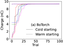
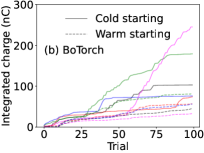
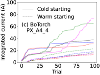
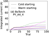
Figure 3 shows the results of the TPE algorithm. We performed a beam-tuning experiment using BoTorch on June 2, 2023, 11 am–3 pm, and an experiment using the TPE on the same day, 3–6 pm; the change in the Linac conditions between the two was negligible.

The five runs indicated by the solid line in panel (a) reached $9\text{\,}\mathrm{nC}$ around the 40th trial and the maximum charge around the 60th trial. The maximum charge was slightly lower than $9.2\text{\,}\mathrm{nC}$, which was in fact $0.1\text{\,}\mathrm{nC}$ lower than the result achieved by BoTorch (see Fig. 2 (a)). The dashed lines in panel (a) show the cases of “warm starting.” Ten combinations of the applied currents were obtained from the cold-starting BoTorch results shown in Fig. 2 (a). As expected from the superior combinations, the maximum charge of the warm-starting runs in Fig. 3 (a) exceeded $9.3\text{\,}\mathrm{nC}$.

Panel (b) shows that the integrated charge obtained by the cold-starting TPE was generally higher than that of BoTorch, as shown in Fig. 2 (b), regardless of whether cold or warm starting was used. Based on panels (b)–(d), the TPE algorithm might focus more on exploration than exploitation and thus reach its maximum charge slower than BoTorch. In panel (b), we observed that up to the 50th trial, the integrated charge for the warm-starting runs was slightly smaller than that for cold-starting runs; however, after the 50th trial, the difference between the two became less prominent. This transition may be because, as shown in panels (c) and (d), the warm-starting TPE algorithm searches a broader range of configuration parameter domains than the cold-starting TPE after initialization. In panels (c) and (d), we observed that the integral applied current of warm starting exceeded that of cold starting around the 30–40th trials.

Figure 3: Results obtained using TPE algorithm. Panel (a) indicates peak hold values of electron-beam charge. Panel (b) indicates integrated charge over trials. Panels (c) and (d) indicate integral applied current for PX_A4_4 and PY_A4_4, respectively.

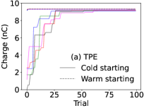
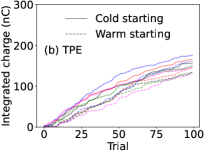
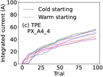
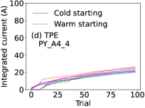
Figure 4 shows the experimental results obtained using the CMA-ES. The measurements were performed on June 12, i.e., 10 days after the BoTorch measurements, as shown in Fig. 2, and the TPE measurements are shown in Fig. 3. During those 10 days, the situation downstream of the electron-beam direction changed, and the beam charge arriving at the most upstream pulsed steering magnet, PX(Y)_A4_4, decreased. Therefore, the maximum charge obtained via the CMA-ES was lower, i.e., below $9\text{\,}\mathrm{nC}$. In panel (a), the solid lines for the cold-starting case shows the maximum charge increasing the most slowly among the three algorithms considered. The dashed lines show the warm-starting case, where the 10 combinations of the applied currents were obtained from the cold-starting CMA-ES measurements (i.e., one of the solid lines). As shown in panels (b)–(d), the integrated charge and applied current were consistently lower for warm starting than for cold starting. This tendency indicates that, as with BoTorch, in the case of warm starting, the optimized applied current is enqueued as the initial value combination and the surrounding domain of that combination is exploited.

The three algorithms, shown in Figs. 2–4, were terminated after 100 trials. However, for BoTorch and the TPE, only one run each was tested, and the optimization was extended to 300 trials. Based on the results, BoTorch continued to be optimized, thus emphasizing exploitation near the maximum charge. However, the TPE shifted from exploitation to exploration after the 150th trial. Systematic measurements based on a significantly higher number of runs shall be attempted in future studies.

Figure 4: Results obtained using CMA-ES algorithm. Panel (a) indicates peak hold values of electron-beam charge. Panel (b) indicates integrated charge over trials. Panels (c) and (d) show integrated applied currents for PX_A4_4 and PY_A4_4, respectively.

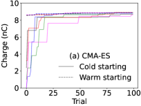
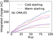
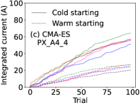
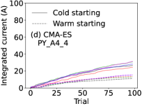
Figure 5 shows the empirical distribution function (EDF), which is defined as

$$F(q_{\textrm{thr}})=\frac{\textrm{number of trials of }q<q_{\textrm{thr}}}{100}=\frac{1}{100}\sum_{i=1}^{100}\mathds{1}_{q<q_{\textrm{thr}}}.$$ (13)

Panel (a) shows the results of the BoTorch algorithm averaged over five runs for the cold-starting (solid line) and warm-starting (dashed line) cases. Each line shows a steep increase in the EDF beginning at approximately $8.5\text{\,}\mathrm{nC}$, thus indicating that many trials yielded a beam charge exceeding $8.5\text{\,}\mathrm{nC}$. For cold starting, approximately $60\text{\,}\mathrm{\char 37\relax}$ of the trials were distributed above $8.5\text{\,}\mathrm{nC}$, whereas for warm starting, approximately $80\text{\,}\mathrm{\char 37\relax}$ of the trials were distributed above $8.5\text{\,}\mathrm{nC}$. The results shown in panel (a) are consistent with the superior performance of BoTorch shown in Fig.. 2.

Panel (b) shows the results of the TPE measured on the same day as that of BoTorch. For a specified beam charge, the warm-starting TPE (dashed line) consistently showed a lower EDF than the cold-starting TPE (solid line), thus indicating that the warm-starting trials were distributed at a slightly higher beam charge. However, the shapes of the EDFs were almost identical, and the differences were insignificant compared with those of BoTorch and the CMA-ES. Slight differences between the two curves suggest that the warm-starting TPE affects the maximum charge through initialization but negligibly affects the trade-off between exploration and exploitation. This trend is consistent with the integrated charge and applied current distributions shown in Figs. 3 (b)–(d).

Panel (c) shows the measurement results obtained using the CMA-ES, where the EDF integrated from 0 to $8\text{\,}\mathrm{nC}$ for cold starting was the largest among the three algorithms considered. Similar to the results shown in Fig. 4 (a), the CMA-ES algorithm for cold starting performed an exploration-oriented optimization in this experiment. However, for warm starting, more than $70\text{\,}\mathrm{\char 37\relax}$ of the trials occurred at $8\text{\,}\mathrm{nC}$ or higher, thus indicating that the optimization focused on exploitation. The trends in panel (c) are similarly shown in Figs. 4 (b)–(d) for warm starting (dashed line).

Figure 5: Empirical distribution functions (EDF) averaged over five runs. Panels (a), (b), and (c) show results of BoTorch, TPE, and CMA-ES, respectively.

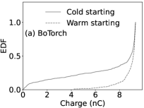
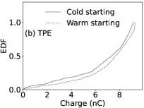
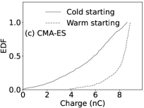
Figure 6 shows the importance of each parameter, namely, the effectiveness of the applied currents in increasing the beam charge. The importance of the parameters can be quantified using a method proposed in Ref. [21], which is based on a random forest prediction model [22] and functional analysis of variance (fANOVA). First, a random-forest model was established to predict the average algorithm performance over the configuration domain. Subsequently, the fANOVA decomposes the variance of the overall algorithm performance into additive components, with each corresponding to a subset of the algorithm parameters. Finally, the fraction of variance associated with each subset of parameters relative to the overall performance variance quantifies the importance of the corresponding subset.

Panel (a) shows the results of the BoTorch measurements. The black circles and red squares represent the average of five cold- and warm-starting runs, respectively. For cold starting, the maximum importance was $\sim 0.5$ for pulsed steering magnet PX_A4_4. Because the importance was normalized such that the sum was 1, PX_A4_4 alone appeared to have contributed to approximately $50\text{\,}\mathrm{\char 37\relax}$ of the importance. As shown in Fig. 1, PX_A4_4 was the most upstream of the three horizontal magnets used in the beam-tuning experiment. Therefore, PX_A4_4 is expected to exert the most significant effect on the horizontal orbit modification, thus resulting in a higher importance for the objective function (i.e., beam charge). Because of a sizable orbit error in the horizontal direction, the beam established contact with the beam collimator in the arc R sector, thus resulting in a significant beam-charge loss. This may explain the higher importance of the horizontal direction PX_A4_4 compared with that of the vertical direction PY_A4_4. For warm starting, the importance of PY_A4_4 increased to 0.4. As shown by the integrated charge in Fig. 2 (b), the integrated applied current in Figs. 2 (c) and (d), and the EDF in Fig. 5 (a), most of the 100 parameter sets for warm starting did not change significantly from the best parameter set that yielded the maximum charge. That is, the applied current of PY_A4_4, which was located upstream, was almost optimized immediately after the initialization. Thus, a slight change in the applied current significantly affected the beam charge loss and became more important. In two locations in the R sector, the vertical beta function exceeded $100\text{\,}\mathrm{m}$. In addition, an electron beam generated by the thermionic DC gun indicated a large emittance. Therefore, if the beam orbit is shifted vertically, then a portion of the bunch with a large transverse size hits the beam pipe, thus resulting in beam-charge loss.

Panel (b) presents the TPE results. The results of cold and warm starting were similar. As shown in Figs. 3 (b)–(d) and Fig. 5 (b), the trade-off between exploitation and exploration changed only slightly, regardless of whether cold or warm starting was used in TPE. Thus, we can assume that the importance of each parameter is similarly distributed for both the cold- and warm-starting runs. Because the TPE optimizes with emphasis on exploration even for warm starting, the results achieved are comparable to those yielded by BoTorch for cold starting.

Panel (c) presents the CMA-ES results. The results for warm starting were comparable to those of BoTorch, which is as expected owing to the similarity of the EDFs shown in Figs. 5 (a) and (c). Meanwhile, the importance of PX_A4_4 for cold starting exceeded 0.7 for the CMA-ES, as compared with 0.5 for BoTorch. Although we have yet to achieve quantitative understanding, we hypothesize that the anti-correlation between the more critical PX_A4_4 and less critical PX_R0_01 may affect the importance of PX_A4_4. Based on panels (a) and (b), the importance of PX_R0_01 is 0.15–0.2, whereas it is less than 0.1 in panel (c).

Figure 6: Importance of each input parameter averaged over five runs. Panels (a), (b), and (c) show results of BoTorch, TPE, and CMA-ES, respectively.

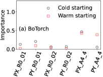
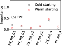
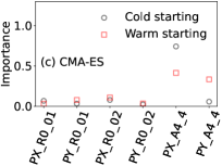
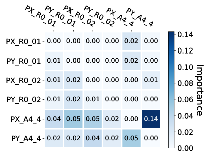
Figure 7 shows the importance of the two-parameter combinations. The results yielded by the warm-starting BoTorch and warm-starting TPE are shown above and below the diagonal line, respectively. For simplicity, we set the values on the diagonal line to zero. In the BoTorch results, the combination of PX_A4_4 and PY_A4_4 showed the highest importance of $\sim 0.14$. Combining the results for warm starting (black squares) in Fig. 6 (a), we observed that the order of importance from highest to lowest was PX_A4_4, PY_A4_4, the combination of both, and the other parameters.

Meanwhile, the importance of the other pulsed steering magnets and their combinations was less than 0.1. The TPE results below the diagonal line show that the importance for the combination of each parameter was 0.05 at the maximum. PY_A4_4 was less critical in the TPE, even for warm starting, as shown in Fig. 6 (b). Consequently, the combination of PX_A4_4 and PY_A4_4 was less critical.

Figures6 and 7 show that the applied currents of PX_A4_4 and PY_A4_4, which were the most upstream pulsed steering magnets used in the experiment, functioned similarly as the other steering magnets for the three algorithms. Therefore, only the applied currents of PX_A4_4 and PY_A4_4 appeared to be sufficient for the enqueued initial parameter values considered under warm starting.

In the next beam-tuning experiment, we plan to perform beam tuning at different sectors of Linac using other magnets and other types of objective functions to obtain more general insights into machine learning-assisted beam tuning.

Figure 7: Importance of each input parameter combination. Numbers shown above and below diagonal line indicate BoTorch and TPE results, respectively. Both results are for warm starting.

IV Multiobjective optimization

This section provides an overview of the methodology of multiobjective optimization, i.e., the case in which multiple objective functions are optimized simultaneously. The $M$-dimensional multiple-objective functions are denoted as $f^{(1)},f^{(1)},\ldots,f^{(M)}$. In the beam-tuning experiment, we set $M=2$ to accommodate the two objective functions (maximization of the beam charge and minimization of the dispersion function). For simplicity, we assume that the goal of multiobjective optimization is to maximize all dimensions.

The simultaneous optimization of multiobjective functions can be redefined as obtaining all the Pareto optimal solutions. To illustrate the Pareto optimal solution, we define the dominance relation. For the two objective functions $\bm{f}(\bm{x})$ and $\bm{f}(\bm{x^{\prime}})$, the relation

$$\bm{f}(\bm{x})\succeq\bm{f}(\bm{x^{\prime}})\Leftrightarrow\forall m\in\{1,\ldots,M\}f^{(m)}(\bm{x})\geqq f^{(m)}(\bm{x^{\prime}})$$ (14)

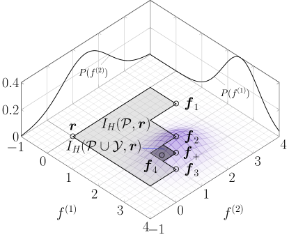
indicates that $\bm{f}(\bm{x})$ dominates $\bm{f}(\bm{x^{\prime}})$ if $f^{(m)}(\bm{x})$ is greater than or equal to $f^{(m)}(\bm{x^{\prime}})$ for all dimensions. Here, $\bm{x}_{i}$ represent the input variables (applied currents of the pulsed steering magnets) and $\bm{f}_{i}$ the objective functions (a beam charge and a dispersion function). The last inequality is presented in Eq. (14) as we are addressing a maximization problem. For example, as shown in Fig. 8, $\bm{f}_{+}$ dominates $\bm{f}_{4}$. We regard $\bm{f}$ as a Pareto-optimal solution when no other point in the objective function space dominates $\bm{f}$. Generally, more than one Pareto-optimal solution exists for multiple objective functions.

The Pareto front is the surface created when plotting the Pareto solution set. Multiobjective optimization aims to efficiently obtain many Pareto-optimal solutions near the Pareto front by discounting the superiority or inferiority of the multiple Pareto-optimal solutions. To obtain the Pareto front, we introduce a Pareto hypervolume. Let $\mathcal{D}=\{(\bm{x}_{i},\bm{f}_{i})\}_{i=1}^{N}$ denote the current dataset, where $N$ is the dataset size. The Pareto front in the data set $\mathcal{D}$ expands with each data addition.

Once a reference point is determined to evaluate the expansion, a hyperrectangle can be defined using the reference point $\bm{r}$ and the Pareto solution set $\mathcal{P}\in\mathcal{D}$.

$$\cup_{i=1}^{\mathcal{P}}[\bm{r},\bm{f}_{i}].$$ (15)

The hypervolume indicator in Eq. (15) is the $M$-dimensional Lebesgue measure, which is expressed as

$$I_{H}(\mathcal{P},\bm{r})=\lambda_{M}(\cup_{i=1}^{\mathcal{P}}[\bm{r},\bm{f}_{i}]).$$ (16)

The shaded light-gray area in Fig. 8 shows the hypervolume indicator with the Pareto solution set $\mathcal{P}=\{(\bm{x}_{i},\bm{f}_{i})\}_{i=1}^{3}$, and reference point $\bm{r}$. The hypervolume indicator increases monotonically for each additional data point. The shaded dark-gray area shows an increase in the hypervolume indicator owing to new observations $\mathcal{Y}=(\bm{x}_{+},\bm{f}_{+})$. Based on this increase, we can define an acquisition function, i.e., the expected hypervolume improvement (EHVI), which is the expected increment in the hypervolume indicator before and after obtaining a new observation $\mathcal{Y}$.

$$\mathit{EHVI}(\mathcal{Y},\mathcal{P},\bm{r})=\\ \int\left(I_{H}(\mathcal{P}\cup\mathcal{Y},\bm{r})-I_{H}(\mathcal{P},\bm{r})\right)p(\bm{f}_{+}\mid\bm{x}_{+},\mathcal{D})d\bm{f}_{+}.$$ (17)

The posterior $p(\bm{f}_{+}\mid\bm{x}_{+},\mathcal{D})$, which is the distribution indicated by the blue surface in Fig. 8, is approximated via a Gaussian process in the Bayesian optimization. Analogous to the single-objective optimization, as discussed in Sec. II, the location $\bm{x}$ that maximizes the acquisition function EHVI is selected and then input to the objective function to advance the Pareto front. The methodology described above assumes a multiobjective Bayesian optimization. A detailed description of this multiobjective optimization based on the TPE algorithm is provided in Refs. [23, 24].

Figure 8: Example of hypervolume indicator $I_{H}$ with Pareto solution set $\{(\bm{x}_{i},\bm{f}_{i})\}_{i=1}^{3}$.

V Application to beam charge and dispersion simultaneous optimization

V.1 Experimental setup at KEK Linac

To investigate the feasibility of applying multiobjective Bayesian optimization to accelerator tuning, we attempted to simultaneously maximize the electron-beam charge and minimize the dispersion function.

The unexpected dispersion function in the Linac and beam-transport line increases the emittance of the injection beam and further reduces the injection efficiency to the light source storage rings (PF and PF-AR) and SuperKEKB [12] downstream of the beam-transport line. Therefore, the beam must be adjusted such that the sizable dispersion function in sector R (see Fig. 1) does not leak downstream.

In this beam-tuning experiment, we used an electron beam generated by a thermionic DC gun dedicated for positron generation. Notably, the dispersion function in sector 1 does not significantly affect positron generation in the actual operation. We attempted to minimize the dispersion function in this experiment such that better electron beams would be received by the PF, PF-AR, and SuperKEKB. Notably, the electron beam generated by the RF electron gun was supplied to the PF and PF-AR when this experiment was conducted and was not used in this study.

In this study, the dispersion function was not used as an objective function. Instead, the following dispersion-position function was used for simplicity, which multiplies the square of the dispersion function by the sum of the squares of the horizontal and vertical positions.

$$f_{\textit{disp-pos}}=\sum_{i=1}^{14}(\eta_{x,i}^{2}+\eta_{y,i}^{2})\sum_{j=1}^{14}(d_{x,j}^{2}+d_{y,j}^{2}).$$ (18)

The dispersion functions and beam positions were measured using 14 BPMs. Additionally, the square value instead of the absolute value in Eq. (18) was adopted to limit the outliers. The product of the dispersion function and position was adopted to simultaneously reduce both the dispersion function and beam-orbit residual. The dispersion function at each BPM location was measured using the inevitably occurring beam-energy jitter. Compared with the case where the dispersion function is measured by intentionally changing the energy-adjustment knob, the method using energy jitter enables measurements to be performed while the beam is being supplied to the light source storage rings or SuperKEKB because the adjustment knob is fixed. However, the energy-jitter method relies on randomly generated jitter and requires a long measurement time to obtain sufficient resolution. In this experiment, 100 data points were required after the pulsed magnet settings were changed. Because the beam repetition rate was $1\text{\,}\mathrm{Hz}$, a waiting period of $100\text{\,}\mathrm{s}$ was permitted after the magnet settings were changed.

V.2 Experimental results

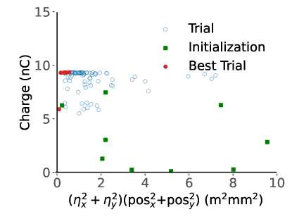
Figure 9 shows the scatter plots of the obtained beam charge vs. the dispersion-position function in Eq. (18) for each trial. Measurements were performed on June 1, 2023, 2–4 am, with 100 trials performed using the BoTorch algorithm. The green squares indicate the 10 trials performed until the end of initialization, the blue open circles indicate the 11th to 100th trials, and the red dots are the Pareto-optimal solution set (five points in total). The initialization explores the beam charge and dispersion-position function domain more extensively than the pairs obtained after the initialization. The beam charges were generally distributed above $6\text{\,}\mathrm{nC}$, and the charge optimization was efficient. Meanwhile, the dispersion-position function exhibited a tail exceeding $2\text{\,}{\mathrm{m}}^{2}\text{\,}{\mathrm{mm}}^{2}$, which can be further improved. Although not used in this study, optuna implements a constrained optimization function. If either the dispersion function or beam-orbit position is constrained, then the optimization can focus of regions where the dispersion-position function is small, e.g., smaller than $1\text{\,}{\mathrm{m}}^{2}\text{\,}{\mathrm{mm}}^{2}$.

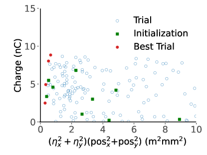
Figure 10 shows a scatter plot of the beam charge vs. dispersion-position function obtained using the TPE algorithm via 200 trials. The result indicates an exploration-oriented optimization of both the beam charge and dispersion-position function, unlike the BoTorch result presented in Fig. 9. This trend is consistent with TPE’s focus on exploration instead of exploitation, as discussed in Sec. III.2. The TPE algorithm data were obtained on June 12, 2023, 6–10 pm; therefore, the beam conditions may have changed since June 1 when we conducted the beam test using the BoTorch algorithm.

As shown in Figs. 9 and 10, we obtain Pareto-optimal solutions for both algorithms. Only a few Pareto-optimal solutions were available for 100 or 200 trials, thus clearly indicating a low-cost performance in terms of the beamtime. The Pareto-optimal solution must be obtained promptly for time-consuming measurements, e.g., more than 60 s per measurement, as in the current tuning experiment. In the future, we plan to test the efficiency of obtaining Pareto-optimal solutions using a constrained optimization algorithm.

Figure 9: BoTorch result for multiobjective optimization on beam charge (vertical axis) and dispersion-position function (horizontal axis).

Figure 10: TPE result for multiobjective optimization on beam charge (vertical axis) and dispersion-position function (horizontal axis).

VI Conclusions

We conducted beam-tuning experiments at the KEK Linac using Bayesian optimization (BoTorch), a TPE, and the CMA-ES to determine the feasibility of using machine learning, in particular optimization algorithms.

In a single-objective optimization experiment to maximize the electron-beam charge from sector C to sector 1 of the Linac, the beam orbit was adjusted by optimizing the applied current of six pulsed steering magnets. The maximum beam charge obtained in the beam-tuning experiment was comparable to that obtained in previous experiments. Approximately 35 trials (10 of which pertained to initialization) were required to reach the maximum beam charge when using the cold-starting BoTorch. On average, the TPE and CMA-ES achieved a lower beam charge under cold starting compared with BoTorch, even after 100 trials. Under warm starting, BoTorch and the CMA-ES showed excellent optimization performance from the initialization phase, where the enqueued initial values were utilized; however, the optimization performance of the TPE under warm starting did not differ significantly from that of cold starting. We conclude that the proposed optimization algorithm can replace manual tuning by experts for beam-charge maximization using steering magnets.

Multiobjective optimization was tested to simultaneously maximize the beam charge and minimize the dispersion-position function. The multiobjective optimization task was to obtain as many effective Pareto-optimal solutions as feasible. The dispersion function was measured using the inevitable beam energy jitter. Two algorithms, i.e., BoTorch and the TPE, were used, and their results were compared. As shown in the single-objective optimization results, the beam charge vs. dispersion-position function distribution was exploitation-oriented for BoTorch and exploitation-oriented for the TPE. Both algorithms yielded four to five Pareto-optimal solutions over 100–200 trials. The efficiency of obtaining the optimal solution is essential for applying multiobjective optimization to accelerator tuning, where each trial is time consuming and hence expensive. In the next test, we shall introduce a constrained optimization algorithm to improve the efficiency of obtaining the optimal solution. In addition, the number of parameters shall be increased to approximately 20 to assess the applicability of multivariable optimization to beam tuning.

The machine-learning-based beam-tuning tool developed for this experiment will be applied to the beam tuning of the SuperKEKB (e.g., beam injection from the beam-transport line to the main ring, correction for horizontal and vertical couplings, and adjustment of the beam collimator head position).