Residual Quantization
with Implicit Neural Codebooks

Abstract

Vector quantization is a fundamental operation for data compression and vector search. To obtain high accuracy, multi-codebook methods increase the rate by representing each vector using codewords across multiple codebooks. Residual quantization (RQ) is one such method, which increases accuracy by iteratively quantizing the error of the previous step. The error distribution is dependent on previously selected codewords. This dependency is, however, not accounted for in conventional RQ as it uses a generic codebook per quantization step. In this paper, we propose QINCo, a neural RQ variant which predicts specialized codebooks per vector using a neural network that is conditioned on the approximation of the vector from previous steps. Experiments show that QINCo outperforms state-of-the-art methods by a large margin on several datasets and code sizes. For example, QINCo achieves better nearest-neighbor search accuracy using 12 bytes codes than other methods using 16 bytes on the BigANN and Deep1B dataset.

Matthijs Douze () and Jakob Verbeek () [Code]https://github.com/facebookresearch/QINCo

1 Introduction

Vector embedding of different data types, e.g. from text (Schwenk and Douze, 2017; Devlin et al., 2018; Izacard et al., 2022) or images (Pizzi et al., 2022; Ypsilantis et al., 2023; Radford et al., 2021), is a pervasive component of many machine learning systems for analysis tasks, recognition, search, matching, and many others. In similarity search and recommender systems (Paterek, 2007), representing entities with embedding vectors is efficient as it enables simple vector comparison. In this context, many techniques and libraries have been developed to search in large collections embedding vectors (Malkov and Yashunin, 2018; Douze et al., 2024; Guo et al., 2020; Morozov and Babenko, 2019). In our work we consider the data embedding approach is fixed, but the resulting vectors need to be compressed for storage, search, or transmission. Lossy vector codecs leverage a quantizer that maps a continuous-domain vector to a code: a (possibly fixed-sized) bit vector. This process induces distortion, measured as the difference between the uncompressed vector and its decoded approximation. A fundamental trade-off exists, where lower rate introduces higher distortion (Cover and Thomas, 1991).

Figure 1: Overview of the QINCo architecture. Top: The reconstructed vector $\hat{{\bm{x}}}$ is obtained in $M$ sequential steps from the code ${\bm{i}}=(i^{1},\dots,i^{M})$. Bottom: Step $m$ involves a look-up from a table with the element $i^{m}$, that is concatenated with the previous estimate $\hat{{\bm{x}}}^{m}$ and transformed with residual MLPs to produce $\hat{{\bm{x}}}^{m+1}$. At decoding time, each step uses the provided $i^{m}$ index. At encoding time, all $i^{m}$ values are tested and the one that yields the $\hat{{\bm{x}}}^{m}$ that best approximates ${\bm{x}}$ is selected.

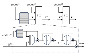
We focus on vector quantization (VQ) (Gray, 1984), which aims to represent a vector with a nearby “prototype” vector. Effective quantizers adapt to the vector distribution by learning a codebook of centroids from a representative set of training vectors. The well-known k-means algorithm leverages this strategy and tends to be near-optimal, but it does not scale well for codes larger than a few bytes, as the number of centroids grows exponentially with the code length. Multi-codebook quantizers (MCQ) yield a tractable alternative. Seminal MCQ techniques —such as product quantization (PQ), residual quantization (RQ) and additive quantization (AQ)— are based on clustering and linear algebra techniques (Jégou et al., 2010; Babenko and Lempitsky, 2014; Martinez et al., 2016, 2018; Chen et al., 2010), while more recent approaches rely on deep neural networks for this purpose (Morozov and Babenko, 2019; Zhu et al., 2023; Niu et al., 2023). However, due to quantization being inherently non-differentiable, gradient-based optimization of such networks tends to be difficult, and involves biased and/or noisy gradient estimation techniques. Codebook collapse (Huh et al., 2023), which causes many codebook vectors to remain unused, is a well-known challenge in such models as well.

Conventional RQ (Chen et al., 2010), which is a special case of AQ, quantizes in each step the residual between the original vector and its reconstruction based on the previous quantization steps. In this paper, we propose a neural variant of RQ. Our method is based on the observation that the residual distribution depends on the selected quantization vectors in earlier steps, which makes it sub-optimal to use fixed codebooks as in conventional RQ. To account for a varying residual distribution, we propose to update the codebook in each step per data point. To this end we leverage a neural network that is conditioned upon the vector reconstruction from the previous steps and a pre-trained RQ base-codebook. We call our method QINCo for Quantization with Implicit Neural Codebooks. See Fig. 1 for a schematic overview.

In contrast to earlier neural MCQ methods, such as (Morozov and Babenko, 2019), QINCo transforms the codebook vectors rather than the vectors to be quantized. Therefore, codebook assignment happens in the original data space and does not require gradient estimation to propagate through the quantization operation. This makes QINCo’s training simple and stable. The similarity of QINCo to a standard RQ enables combining it with inverted file indexes (IVF) (Jégou et al., 2010) and re-ranking techniques for fast approximate decoding. This renders QINCo suitable as well for highly accurate large-scale similarity search. Our contributions can be summarized as follows:

• We introduce QINCo, a neural residual vector quantizer that — instead of using fixed codebooks — adapts quantization vectors to data points. It is stable to train and has few hyperparameters.

• QINCo sets state-of-the-art performance for vector compression on multiple datasets and rates, and thanks to its compatibility with fast approximate search techniques, it also beats state-of-the-art similarity search performance for high recall operating points.

• QINCo codes can be decoded from the most to the least significant byte, with prefix codes yielding accuracy on par with codes specifically trained for that code length, making QINCo an effective multi-rate codec.

2 Related work

Vector quantization. A vector quantizer maps a vector ${\bm{x}}\in\mathbb{R}^{D}$ to a vector taken from a finite set of size $K$ (Gray, 1984). This set is called the codebook, and each codebook entry is referred to as “centroid”, or “codeword”. The objective is to minimize the distortion between ${\bm{x}}$ and its quantization. Lloyd’s algorithm, a.k.a. k-means, uses the squared $\ell_{2}$ distance to measure distortion. Even though obtaining the global optimum of k-means is NP hard, good local minima are accessible in practice. The $K$ centroids output by k-means can be enumerated, leading to codes of size $\lceil\log_{2}(K)\rceil$ bits. K-means, however, only scales well up to a few million centroids, resulting in code lengths in the order of 20 bits, which is too coarse for a practical codec.

Multi-codebook quantization. To scale beyond the inherent limitations of k-means, MCQ was introduced, which uses several k-means quantizers. PQ slices vectors into sub-vectors that are quantized independently (Jégou et al., 2010). AQ, on the other hand, represents each vector as a sum of multiple codebook entries (Babenko and Lempitsky, 2014; Martinez et al., 2016, 2018). RQ progressively quantizes residuals (Chen et al., 2010). A trade-off exists between compression accuracy and encoding speed. PQ enables fast encoding, while AQ is typically more accurate. We build upon RQ, using neural networks to improve its accuracy.

Neural quantization. Neural quantization has been explored to learn discrete image representations, which are then used to leverage discrete sequence models for the generation of images (van den Oord et al., 2017; Esser et al., 2021; Lee et al., 2022; Chang et al., 2022) and audio (Copet et al., 2023). Another line of work uses such models for compression of images (Agustsson et al., 2017; El-Nouby et al., 2023) and audio (Défossez et al., 2023; Kumar et al., 2023). Klein and Wolf (2019) explored a neural variant of PQ for image embeddings, which was trained with a supervised loss based on image class labels. In contrast to all these works, our work focuses on unsupervised neural MCQ for vector compression.

UNQ (Morozov and Babenko, 2019) and DeepQ (Zhu et al., 2023) are neural vector quantization approaches for additive MCQ with trainable codebooks. To overcome challenges regarding gradient estimation of the non-differentiable quantization procedure, both approaches model the selected quantization vector as a sample from a categorical distribution during training, for which gradient estimators exist. DeepQ leverages the REINFORCE estimator (Glynn, 1990; Williams, 1992) with additional control variates to reduce its variance, and UNQ uses the Straight-through-Gumbel-Softmax estimator (Jang et al., 2017; Maddison et al., 2017) with carefully initialized trainable Boltzmann temperatures (Huijben et al., 2022). Both models use the nearest codeword during encoding. Since QINCo encodes in data space, and thus does note have an encoder that needs gradient updates, QINCo does not require gradient propagation through the quantization step. This takes away the need for a gradient estimator. By avoiding the use of an encoder, and initializing QINCo with vanilla RQ, training of QINCo is very stable and does not suffer from codebook collapse. As such it does not require an additional regularizer as used in UNQ and DeepQ, that maximizes the spread of vectors over the codebook.

Re-ranking. It is common practice to accelerate large-scale nearest neighbor search with approximation techniques that rely on a cheap distance measure to select a “shortlist” of nearest neighbors, which are subsequently re-ordered using a more accurate measure. This re-ordering can, e.g., be done using a finer quantizer (Jégou et al., 2011), or in the limit no quantizer (Guo et al., 2020), compared to the one used for creating the shortlist. It is also possible to re-interpret the same codes with a more complex decoding procedure. For example, polysemous codes (Douze et al., 2016) can be compared both as binary codes with Hamming distances, similar to (He et al., 2013), and as PQ codes. UNQ (Morozov and Babenko, 2019) uses a fast AQ for search and re-ranks with a slower decoding network. It has also been shown that in some cases, given a codec, it is possible to train a neural decoder that improves the accuracy (Amara et al., 2022), and use the trained decoder to re-rank the shortlist. To enable fast search with QINCo, we also propose to use a less accurate, but faster linear decoder to create a shortlist for re-ranking, for which —given the QINCo encoder— a closed-form solution is available in the least-squared sense (Babenko and Lempitsky, 2014).

3 RQ with implicit neural codebooks

Before we detail our approach, we briefly review RQ to set some notation; for more details see, e.g., (Chen et al., 2010). We use ${\bm{x}}\in\mathbb{R}^{D}$ to denote vectors we aim to quantize using $M$ codebooks of $K$ elements each. Let $\hat{{\bm{x}}}^{m}$ for $m=1,\dots,M$ be the reconstruction of ${\bm{x}}$ based on the first $m-1$ quantization steps, where we define $\hat{{\bm{x}}}^{1}=\mathbf{0}$. For each quantization stage $m$, RQ learns a separate codebook ${\bm{C}}^{m}\in\mathbb{R}^{D\times K}$ to quantize the residuals ${\bm{r}}^{m}={\bm{x}}-\hat{{\bm{x}}}^{m}$, by applying k-means separately for each level. We denote the individual codebook elements in the columns of ${\bm{C}}^{m}$ as ${\bm{c}}^{m}_{k}$ for $k=1,\dots,K$. To encode ${\bm{x}}$, the partial data reconstruction is recursively updated according to $\hat{{\bm{x}}}^{m+1}=\hat{{\bm{x}}}^{m}+{\bm{c}}^{m}_{i^{m}}$, where $i^{m}={\arg\min}_{k=1,\dots,K}\left\lVert{\bm{r}}^{m}-{\bm{c}}_{k}^{m}\right\rVert^{2}_{2}$. The $M$ quantization indices ${\bm{i}}=(i^{1},\dots,i^{M})$ are finally stored to represent ${\bm{x}}$ using $M\log_{2}(K)$ bits. To decode ${\bm{i}}$, the corresponding codebook elements are summed to obtain the approximation $\hat{{\bm{x}}}=\sum_{m=1}^{M}{\bm{c}}^{m}_{i^{m}}$, i.e. RQ has an additive decoder.

3.1 Implicit neural codebooks

At each step of the previously-described RQ scheme, all residuals are quantized with a single step-dependent codebook ${\bm{C}}^{m}$. This is sub-optimal, as in general the distribution of residuals differs across quantization cells. In theory, one could improve upon RQ by proceeding in a hierarchical manner, using a different “local” codebook for each hierarchical Voronoi cell that is adapted to model the data in that cell. In practice, however, as the number of hierarchical Voronoi cells grows exponentially with the number of quantization steps $M$, this is feasible only for very shallow RQs. To sidestep the practical infeasibility of RQ with explicit local codebooks, we leverage neural networks to implicitly represent locally-adaptive codebooks for RQ.

For each quantization step $m$ we train a separate neural network that, given a partial reconstruction $\hat{{\bm{x}}}^{m}$ and a base codeword $\bar{{\bm{c}}}_{k}^{m}$, produces a specialized codeword for the residuals ${\bm{r}}^{m}$ in the corresponding hierarchical Voronoi cell. In this way the same network can be re-used for improving all $K$ vectors in the $m$-th codebook: ${\bm{c}}_{k}^{m}=f(\hat{{\bm{x}}}^{m},\bar{{\bm{c}}}_{k}^{m};\theta_{m})$. This network has and output dimension $D$, and the $K$ specialized codewords can be computed in parallel. The $M$ base codebooks $\bar{{\bm{C}}}=(\bar{{\bm{C}}}^{1},\dots,\bar{{\bm{C}}}^{M})$ are initialized using a pre-trained conventional RQ, and $f(\cdot)$ contains residual connections (He et al., 2016) that let the pre-trained base codebook pass-through, while allowing trainable multi-layer perceptrons (MLPs) to modulate these codebooks. This architecture design prevents spending many training cycles to achieve RQ baseline performance. The base codebooks are made trainable parameters themselves as well, so that $\bar{{\bm{C}}}^{m}\subset\theta_{m}$.

More precisely, the first layer in $f(\cdot)$ projects the concatenation of $\bar{{\bm{c}}}_{k}^{m}$ and $\hat{{\bm{x}}}^{m}$ to a $D$-dimensional space. The MLPs in the subsequent residual blocks all contain two linear layers, with a ReLU activation in between. Note that in the first quantization step we have $\hat{{\bm{x}}}^{1}=\mathbf{0}$ by construction, which does not provide any useful context to condition the codebook-generating network on. As such, we define a simplified architecture for $f(\cdot;\theta_{1})$, which just selects the nearest codebook elements from the trainable base codebook. The number of trainable parameters $|\theta|=\sum_{m}|\theta_{m}|$ in QINCo equals:

$$|\theta|=M\underbrace{KD}_{\bar{{\bm{C}}}^{m}}+(M-1)\big{[}\underbrace{\big{(}2D^{2}+D\big{)}}_{\text{concat. block}}+\underbrace{2LDh}_{\text{residual-MLPs}}\big{]},$$ (1)

with $L$ the number of trainable residual-MLP blocks, and $h$ the hidden dimension of the 2-layer residual-MLPs. See Fig. 1 for an illustration of the architecture.

3.2 Encoding and decoding

Encoding a vector into a sequence of quantization indices proceeds as in conventional RQ encoding, the only difference is that QINCo predicts the $K$ codewords for the $m^{\text{th}}$ codebook as ${\bm{c}}_{k}^{m}=f(\hat{{\bm{x}}}^{m},\bar{{\bm{c}}}_{k}^{m};\theta_{m})$, with $k=1,\ldots,K$, rather than using a fixed codebook per step $m$.

Unlike the conventional RQ decoder, QINCo has a sequential decoding process, as the codebook-generating network is conditioned on the partial reconstructions $\hat{{\bm{x}}}^{m}$. Given an encoding ${\bm{i}}$, and an initial reconstruction $\hat{{\bm{x}}}^{1}=\mathbf{0}$, for each quantizaton step $m=1,\dots,M$, the reconstruction is updated according to $\hat{{\bm{x}}}^{m+1}\leftarrow\hat{{\bm{x}}}^{m}+f(\hat{{\bm{x}}}^{m},\bar{{\bm{c}}}_{i^{m}}^{m};\theta_{m})$, with $\hat{{\bm{x}}}:=\hat{{\bm{x}}}^{M+1}$ being the final reconstruction.

3.3 Training

To train parameters $\theta=(\theta_{1},\dots,\theta_{m})$ we perform stochastic gradient decent to minimize the mean-squared-error (MSE) between each residual and the nearest codebook centroid. For each quantization step, we optimize the following elementary training objective, defined per data point as:

$$\mathcal{L}^{m}(\theta)=\min_{k=1,\dots,K}\left\lVert{\bm{r}}^{m}-f(\hat{{\bm{x}}}^{m},\bar{{\bm{c}}}_{k}^{m};\theta_{m})\right\rVert^{2}_{2}.$$ (2)

Note that both ${\bm{r}}^{m}$ and $\hat{{\bm{x}}}^{m}$ are implicitly dependent on parameters $(\theta_{1},\ldots,\theta_{m-1})$. Therefore, gradients from later quantization steps propagate back to earlier ones as well. The reconstruction is recursively updated as $\hat{{\bm{x}}}^{m+1}=\hat{{\bm{x}}}^{m}+{\bm{c}}^{m}_{i^{m}}$, with assignment $i^{m}={\arg\min}_{k=1,\dots,K}\left\lVert{\bm{r}}^{m}-{\bm{c}}_{k}^{m}\right\rVert^{2}_{2}$. Combining this loss for all $M$ steps yields the final loss:

$$\mathcal{L}_{\textrm{{QINCo}}}(\theta)=\sum_{m=1}^{M}\mathcal{L}^{m}(\theta).$$ (3)

Computationally, the loss just performs an encoding of the training vectors. It avoids costly mining of negative samples for contrastive learning, as done in UNQ (Morozov and Babenko, 2019). In the implementation, we compute the loss in two passes: (1) an encoding of the training batch without tracking the gradients, and (2) computation of the loss with gradients when the codes are known. This speeds up the computation 2.5$\times$ compared to a naive implementation.

4 Large-scale search with QINCo

For nearest-neighbor search in billion-scale datasets it is prohibitive to exhaustively decompress all vectors with QINCo, and compute distances between the query and the decompressed vectors. To accelerate search we combine an inverted index structure (Sec. 4.1) with approximate decoding (see Sec. 4.2) and re-ranking with the QINCo decoder. We refer to this fast search pipeline as IVF-QINCo. This approach gradually refines the search, and concentrates compute on the most promising database vectors.

4.1 Inverted file index (IVF)

A basic technique in large-scale search (Jégou et al., 2010) consists of partitioning the database in ${K_{\mathrm{IVF}}}$ buckets using k-means, and maintaining for each centroid in the resulting codebook a list of all vectors that are assigned to it. Given a query, only data in the ${P_{\mathrm{IVF}}}\ll{K_{\mathrm{IVF}}}$ buckets corresponding to the ${P_{\mathrm{IVF}}}$ centroids closest to the query are accessed.

Similar to how the classical IVFADC indexing (Jégou et al., 2010) uses a PQ to encode the residual of IVF vectors w.r.t. the centroids of the cluster they are assigned to, we integrate IVF with QINCo. When inserting a database vector into the IVF-QINCo index, the first quantization step ($m\!=\!1$) becomes equivalent to the subsequent steps ($m\!>\!1$): it is a codebook-predicting network that is conditioned upon $\hat{{\bm{x}}}^{1}:={\bm{c}}_{i^{\text{IVF}}}$, where ${\bm{c}}_{i^{\text{IVF}}}$ is the IVF centroid the vector is assigned to.

4.2 Approximate decoding

Searching with IVF reduces the number of distance computations by a factor ${P_{\mathrm{IVF}}}/{K_{\mathrm{IVF}}}$. However, compared to PQ and RQ, this does not result in competitive search times yet when combined with QINCo. This is because PQ and RQ, in addition to being cheaper to decode, can benefit from pre-computation of inner products between the query and all codebook elements. Distance computation between the query and a compressed database vector then reduces to summing $M$ pre-computed dot-products per database vector, which amounts to $M$ look-ups and additions (Jégou et al., 2010). Note that, for RQ, when using $\ell_{2}$ distances instead of dot-products for search, the norm of the vectors must also be stored (Babenko and Lempitsky, 2014).

QINCo codebooks are not fixed, so this speed-up by table look-ups can not be applied directly. However, it is possible to fit an additive decoder with fixed and explicit codebooks per quantization level, using quantization indices from our QINCo encoder. This returns approximate distances that can be used to create a short-list of database vectors for which the exact QINCo decoder is applied. More precisely, let ${\bm{G}}=({\bm{G}}^{1},\dots,{\bm{G}}^{M})$ denote a set of $M$ explicit codebooks ${\bm{G}}^{m}\in\mathbb{R}^{D\times K}$, and let ${\bm{g}}^{m}_{k}$ denote the $k$-th element in the $m$-th codebook, we then minimize the MSE loss, defined per data point as:

$$\mathcal{L}_{\mathrm{MSE}}({\bm{G}})=\left\lVert{\bm{x}}-\sum_{m=1}^{M}{\bm{g}}^{m}_{i^{m}}\right\rVert_{2}^{2},$$ (4)

where $\sum_{m=1}^{M}{\bm{g}}^{m}_{i^{m}}$ is the reconstruction of ${\bm{x}}$ using the quantization indices ${\bm{i}}$ produced by the QINCo encoder. This optimization can be solved in closed form (Babenko and Lempitsky, 2014). We refer to this approximate decoder as “AQ decoder”, as opposed the QINCo decoder. While at first it may seem unlikely that this AQ decoder will yield useful reconstructions, it turns out that the reconstructions are accurate enough to pre-select vectors that can be re-ranked using the QINCo decoder. This is likely at least in part due to the initialization of QINCo with vanilla RQ codebooks.

5 Experiments

5.1 Experimental setup

Datasets and metrics. We leverage datasets that vary in dimensionality ($D$) and modality: Deep1B ($D$=96) (Babenko and Lempitsky, 2016) and BigANN ($D$=128) (Jégou et al., 2011) are widely-used benchmark datasets for VQ and similarity search that contain CNN image embeddings and SIFT descriptors, respectively. Facebook SimSearchNet++ (FB-ssnpp; $D$=256) (Simhadri et al., 2022) contains image embeddings intended for image copy detection that were generated using the SSCD model (Pizzi et al., 2022) for a challenge on approximate nearest neighbor search. It is considered challenging for indexing, as the vectors are spread far apart. SIFT1M ($D$=128) (Jégou et al., 2010) is a smaller-scale dataset of SIFT descriptors used for vector search benchmarks. In addition, we introduce the Contriever dataset, that consists of 21M 100-token text passages extracted from Wikipedia, embedded ($D$=768) using the Contriever model (Izacard et al., 2022). This model is a BERT architecture (Devlin et al., 2018) fine-tuned specifically for text retrieval. We randomly split the embeddings in database vectors, queries, and training vectors.

We report compression performance using the mean-squared-error (MSE) on 1M database vectors. To evaluate search performance we additionally report the nearest-neighbor recall percentages at ranks 1, 10 and 100 using 10k non-compressed queries and 1M or 1B compressed database vectors. For resource consumption we focus on parameter counts: since QINCo contains essentially linear layers, the decoding time is proportional to this count, making it a good proxy for run time.

Baselines. We compare QINCo to widely-adopted baselines OPQ (Ge et al., 2013), RQ (Chen et al., 2010), LSQ (Martinez et al., 2018), for which we use implementations in the Faiss library (Douze et al., 2024) with default settings. We also compare to state-of-the-art neural baselines UNQ (Morozov and Babenko, 2019), RVPQ (Niu et al., 2023), and DeepQ (Zhu et al., 2023). RVPQ slices vectors into chunks like PQ and subsequently performs RQ separately in each block rather than using a single quantizer per block. For UNQ, RVPQ and DeepQ we quote performances from the original papers. For UNQ we also reproduced results using the author’s public code, and run additional experiments, see Sec. A.2 for more details.

		BigANN1M		Deep1M		Contriever1M		FB-ssnpp1M
		MSE	R@1	MSE	R@1	MSE	R@1	MSE	R@1
		($\times 10^{4}$)						($\times 10^{4}$)
8 bytes	OPQ	2.95	21.9	0.26	15.9	1.87	8.0	9.52	2.5
	RQ	2.49	27.9	0.20	21.4	1.82	10.2	9.20	2.7
	LSQ	1.91	31.9	0.17	24.6	1.65	13.1	8.87	3.3
	UNQ	1.51	34.6	0.16	26.7	—	—	—	—
	QINCo	1.12	45.2	0.12	36.3	1.40	20.7	8.67	3.6
16 bytes	OPQ	1.79	40.5	0.14	34.9	1.71	18.3	7.25	5.0
	RQ	1.30	49.0	0.10	43.0	1.65	20.2	7.01	5.4
	LSQ	0.98	51.1	0.09	42.3	1.35	25.6	6.63	6.2
	UNQ	0.57	59.3	0.07	47.9	—	—	—	—
	QINCo	0.32	71.9	0.05	59.8	1.10	31.1	6.58	6.4

Table 1: Comparison of QINCo with state-of-the-art methods in terms of reconstruction error (MSE) and nearest-neighbor search recall (R@1) in percentages.

Training details. We run experiments using 500k and 10M training vectors. In all experiments, we hold out an additional set of 10k vectors for validation, except for the smaller SIFT1M dataset for which we always use 95k training vectors and 5k validation vectors. We perform early stopping based on the validation loss. For training, all data were normalized by dividing the vector by the maximum absolute value in the training set.

The number of trainable parameters in QINCo scales linearly with the number of residual blocks $L$ and the hidden dimension $h$ of the residual-MLPs. Preliminary experiments showed that the performance gain of increasing either $L$ or $h$ by the same factor was very similar, see Sec. B.1. Therefore, to vary the capacity of QINCo, we varied the number of residual blocks $L$, and fixed the hidden dimension to $h=256$. For most experiments we use $M\in\{8,16\}$ quantization levels and vocabulary size $K=256$, which we denote as “8 bytes” and “16 bytes” encoding. For more details on our experimental setup see App. A.

	4 bytes			8 bytes
	R@1	R@10	R@100	R@1	R@10	R@100
	SIFT1M
RVPQ	10.2	34.7	74.5	30.3	73.8	97.4
DeepQ	11.0	37.7	76.8	28.0	70.2	96.4
QINCo	14.9	45.5	82.7	35.8	80.4	98.6
	Deep1M
DeepQ	7.4	30.0	72.5	20.9	62.1	94.1
QINCo	9.1	36.3	77.8	25.4	72.1	97.4

Table 2: Recall values at different ranks for similarity search. QINCo with $L\!=\!4$ is reported.

5.2 Quantization performance

In Tab. 1 we compare QINCo against the baselines on four datasets. For Contriever we report QINCo with $L\!=\!12$, for the other datasets we report $L\!=\!16$. QINCo outperforms all baselines on all datasets with a large margin. On BigANN for example, QINCo reduces the MSE by 26% and 44% for 8 and 16 bytes encodings respectively, and we search recall (R@1) is improved by more than 10 points for both encodings. To compare to reported results for DeepQ (Zhu et al., 2023) and RVPQ (Niu et al., 2023) we train a smaller QINCo ($L\!=\!4$) on 100k vectors for Deep1B and 95k vectors for SIFT1M. Tab. 2 shows that QINCo substantially outperforms these methods as well on both datasets. In general we find that QINCo optimally uses all codewords without explicitly enforcing this using regularization during training, see Sec. B.2.

Note that the methods that we compare have different numbers of parameters and training set sizes, and also vary in encoding and decoding speed. These are analyzed in Secs. 5.3 and 5.4.

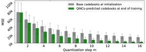
Figure 2 shows that QINCo gains accuracy with respect to the base RQ in all quantization steps, but the improvement is larger in the deeper ones. An explanation is that for deeper quantization steps, the residual distributions tend to become more heterogeneous across cells, so specialized codebooks predicted by QINCo become more useful.

5.3 Search performance

Figure 2: MSE on BigANN1M across 16 bytes quantization steps at initialization of QINCo ($L\!=\!16$), and after training on 10M samples.

	Encoding		Decoding
	FLOPS	time	FLOPS	time
OPQ	$D^{2}+KD$	1.5	$D(D+1)$	1.0
RQ	$KMDB$	8.3	$MD$	1.3
UNQ	$h^{\prime}(D\!+\!h^{\prime}\!+\!Mb\!+\!MK)$	18.8	$h^{\prime}(b\!+\!h^{\prime}\!+\!D\!+\!M)$	13.0
QINCo	$2MKD(D+Lh)$	823.4	$2MD(D+Lh)$	8.3

Table 3: Complexity of encoding and decoding per vector (in floating point operations, FLOPS) and indicative timings on 32 CPU cores (in $\mu$s) with parameters: $D$=128; QINCo: $L$=2, $M$=8, $h$=256; UNQ: $h^{\prime}$=1024; $b$=256; RQ: beam size $B$=5. In practice, at search time for OPQ and RQ we perform distance computations in the compressed domain, which takes $M$ FLOPS (0.16 ns).

In Tab. 3 we report the complexity and corresponding encoding/decoding times of QINCo and baselines. All timings are performed on 32 threads of a 2.2 GHz E5-2698 CPU with appropriate batch sizes. Both the complexity and the timings show that plain QINCo is slower than the competing methods. Given the encoding complexity of QINCo on CPU, we run encoding on GPU for all QINCo experiments not related to timing. The encoding time for the same QINCo model on a Tesla V100 GPU is 28.4 $\mu$s per vector.

Since the search speed depends on the decoding speed of the model, we experiment with approximate decoding for QINCo, as described in Sec. 4.2. For each query we fetch $n_{\mathrm{short}}$ results using the approximate AQ representation and do a full QINCo decoding on these to produce the final search results. Table 4 shows that the R@1 accuracy of the approximate AQ decoding is low compared to decoding with QINCo (and compared to RQ). However, re-ranking the top-1000 results (i.e., 0.1% of the database) of the AQ decoder with QINCo brings the recall within 0.3% of exhaustive QINCo decoding.

	BigANN1M		Deep1M
	8 bytes	16 bytes	8 bytes	16 bytes
AQ	12.7	15.6	11.9	17.6
$n_{\mathrm{short}}=10$	30.5	43.1	25.3	40.3
$n_{\mathrm{short}}=100$	38.9	62.8	30.3	53.0
$n_{\mathrm{short}}=1000$	40.1	67.2	31.2	54.9
QINCo	40.2	67.5	31.1	55.0

Table 4: Search accuracy (R@1) using the approximate AQ decoder only (row 1), AQ in combination with QINCo (with $L\!=\!2$) to re-rank a shortlist of size $n_{\mathrm{short}}$ obtained using the AQ decoder (rows 2, 3, 4), and QINCo to decode the full database (row 5).

Only using approximate decoding to create a shortlist does not render competitive search speeds yet. As such, we experiment with IVF-QINCo on billion-scale datasets, which combines AQ approximate decoding with IVF (see Sec. 4). We use IVF-QINCo with ${K_{\mathrm{IVF}}}$=$10^{6}$ centroids. In terms of pure encoding (i.e. without AQ decoding), IVF-QINCo already improves the MSE of regular QINCo (numbers for $L\!=\!4$):

	BigANN, 8 bytes	BigANN, 16 bytes
QINCo	$1.24\times 10^{4}$	$3.77\times 10^{3}$
IVF-QINCo	$7.80\times 10^{3}$	$2.74\times 10^{3}$

Figure 3: Speed-accuracy trade-off in terms of queries per second (QPS) and recall@1 for IVF-QINCo, on BigANN1B ($10^{9}$ vectors), compared to IVF-PQ and IVF-RQ.

We implement IVF-QINCo in Faiss, starting from a standard IVF index with AQ encoding. For each query, we use HNSW (Malkov and Yashunin, 2018) to search the ${P_{\mathrm{IVF}}}$ nearest centroids (Baranchuk et al., 2018) and do compressed-domain distance computations in the corresponding inverted lists (note that, similar to RQ, this requires one additional byte per vector to encode the norms). We retrieve the top-$n_{\mathrm{short}}$ nearest vectors with approximate distances. Then we run QINCo decoding on the shortlist to compute the final results. See Sec. A.3 for details.

Figure 4: Performance of QINCo of residual blocks $L$ and a training set size $T$ of 10M (solid) or 500k (open).

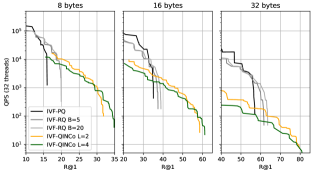
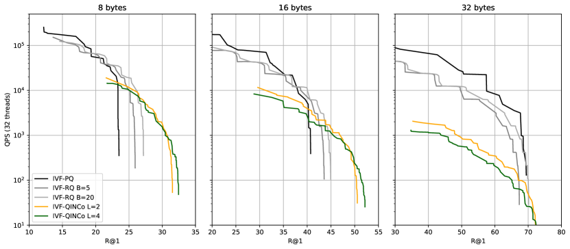
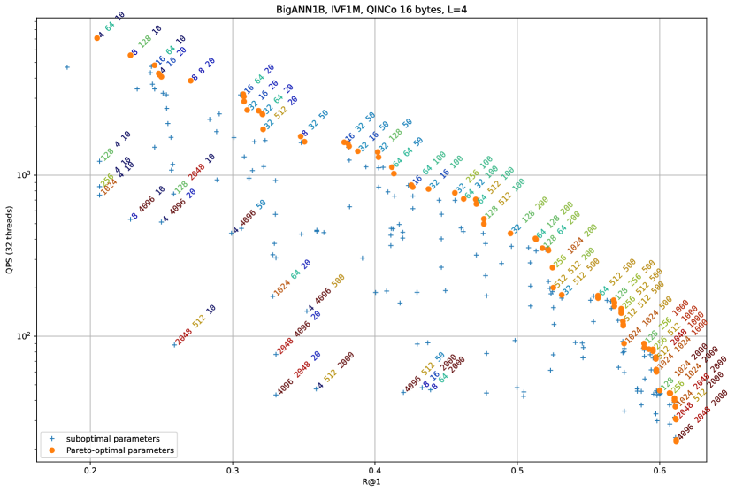
In Fig. 3 we plot the speed-accuracy trade-offs obtained on BigANN1B (database of size $10^{9}$) using IVF-QINCo, IVF-PQ and IVF-RQ. We report IVF-RQ results and IVF-QINCo with two settings of build-time parameters ($L$ and $B$) that adjust the trade-off between encoding time and accuracy. There are three search-time parameters: ${P_{\mathrm{IVF}}}$, $\mathrm{efSearch}$ (a HNSW parameter) and $n_{\mathrm{short}}$. For each method we evaluate the same combinations of these parameters and plot the Pareto-optimal set of configurations. We observe that there is a continuum from IVF-PQ, via IVF-RQ to IVF-QINCo: IVF-PQ is fastest but its accuracy saturates quickly, IVF-RQ is a bit slower but gains about 5 percentage points of recall; IVF-QINCo is again slower but is 10 to 20 percentage points of recall above IVF-RQ. The impact of the build-time parameters is significant but does not bridge the gap between the methods. For the operating points where IVF-QINCo is interesting, it can still sustain hundreds to thousands of queries per second. This is the order of speeds at which hybrid memory-flash methods operate (Subramanya et al., 2019), except that QINCo uses way less memory. Section B.4 presents additional analyses on fast search with IVF-QINCo.

5.4 Further analysis

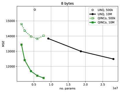
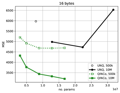
Scaling experiments. To investigate the interaction between training set size and model capacity, we train QINCo on both 500k and 10M vectors for 8 and 16 byte codes, and vary the number of residual blocks $L$. Fig. 4 shows that in all cases the accuracy significantly improves with more training data, and that given enough training data it keeps improving with larger model capacity $L$. For less training data, (500k vectors), increasing the capacity too much degrades the accuracy, due to overfitting.

To test whether baselines benefit similarly from more training data, we train OPQ, RQ and LSQ on 10M training vectors. Table S4 in Sec. B.6 shows that these algorithms hardly benefit from more training data. UNQ was originally trained on 500k training vectors using shallow encoder and decoder designs: both only contained a two-layer MLP with $h^{\prime}\!=\!1024$ hidden dimensions. We found that when increasing either the depth ($L^{\prime}$) or width ($h^{\prime}$) of these MLPs, while training on 500k vectors, UNQ suffers from overfitting and test performance decreases (also when deviating from the hyperparameter settings given by the authors). However, when training on 10M vectors, the MSE improves with an increased hidden dimension and number of layers in the MLPs. Nevertheless, when plotting the number of trainable parameters to MSE performance, Fig. S6 in Sec. B.6 shows that the Pareto front of these better-performing UNQ models remains far from QINCo’s performance.

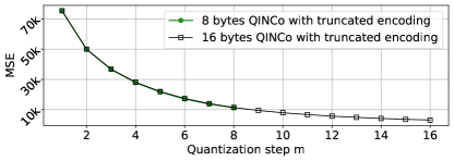
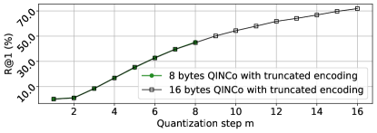
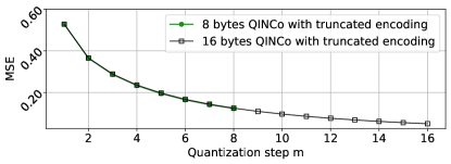
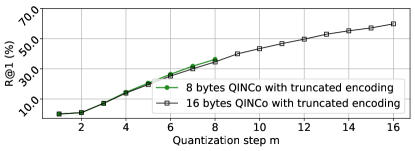
Dynamic Rates. We evaluate whether a QINCo model trained for long codes can be used to generate short codes, or equivalently, if partial decoding can be performed by stopping the decoding after $m<M$ steps. Fig. 5 shows the MSE per quantization step on BigANN1M for both the 8 and 16 bytes models ($L\!=\!16$). The MSE after the $m$-th quantization step is almost identical for both models. This has several benefits: compressed domain rate adjustment (vectors can be approximated by cropping their codes); amortized training cost (train only once for the largest $M$ required); simple model management (only a single model is required). This also implies that the loss at step $m$ hardly influences the trainable parameters in steps $<m$. Sec. B.3 shows similar graphs for Deep1B and the R@1 metric for both datasets. They show that with 12 bytes and more, QINCo outperforms 16-byte-UNQ’s R@1=59.3% for BigANN1M and R@1=47.9% for Deep1M.

Figure 5: The MSE after the $m^{\text{th}}$ quantization step is very similar for the 8 bytes and 16 bytes models for BigANN1M.

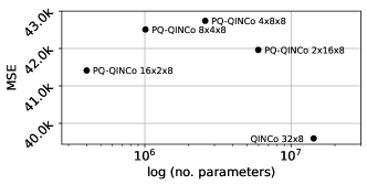
Integration with product quantization. For efficiency when generating large codes, RQ is often combined with PQ to balance sequential RQ stages with parallel PQ coding (Babenko and Lempitsky, 2015; Niu et al., 2023). In this setup, the vector is divided into sub-vectors, and an RQ is trained on each sub-vector. QINCo can equivalently be combined with PQ. We train QINCo and PQ-QINCo ($L\!=\!2$) on 10M vectors of FB-ssnpp for 32 bytes encoding. Fig. 6 shows the trade-off between number of parameters and performance between PQ-QINCo and QINCo. Interestingly, using more PQ blocks deteriorates performance until a turning point, where performance improves again. Vanilla PQ (Jégou et al., 2010) has 65.5k trainable parameters (way fewer than the PQ-QINCo variants) and obtains MSE=55.7k (much worse than PQ-QINCo). Thus, compared to QINCo, PQ-QINCo speeds up encoding and search in high-rate regimes, at the cost of some accuracy.

Figure 6: Comparing 32 byte encodings of FB-ssnpp for QINCo and PQ-QINCo. The setting $16\times 2\times 8$ means we use 16 PQ blocks, $M\!=\!2$ residual stages and $K\!=\!2^{8}\!=\!256$ centroids.

QINCo variant for high-dimensional data. The number of trainable parameters in QINCo scales in $\mathcal{O}(D^{2})$, see equation 1. For high-dimensional embeddings, we propose QINCo-LR, a variant of QINCo that contains an additional low-rank (LR) projection: for each QINCo step, we replace the first linear layer $\mathbb{R}^{2D}\rightarrow\mathbb{R}^{D}$ by two linear layers that map $\mathbb{R}^{2D}\rightarrow\mathbb{R}^{h}\rightarrow\mathbb{R}^{D}$. QINCo-LR scales in $\mathcal{O}(hD)$. We fix $h\!=\!256$ (same as the residual blocks) and compare QINCo-LR (8 bytes; $L\!=\!4$) trained on 10M Contriever embeddings to vanilla QINCo:

	number of parameters	MSE
QINCo	20.85M	1.45
QINCo-LR	16.71M	1.46

In this case, QINCo-LR is 20% more parameter-efficient, while barely loosing performance. QINCo-LR is thus interesting for even larger embeddings, as more than 1,000 dimensions is not uncommon (Oquab et al., 2023; Devlin et al., 2018).

Allocating bits. Given a fixed bits budget $M\log_{2}(K)$, PQ and additive quantizers are more accurate with a few large codebooks (small $M$, large $K$) than with many small codebooks (large $M$, small $K$), as the latter setting has a lower capacity (fewer trainable parameters). To investigate whether QINCo behaves similarly, we train QINCo ($T=500\textrm{k},L\!=\!4$, and a base learning rate of $10^{-3}$) on BigANN1M with $M\!=\!10$ codebooks with the default $K\!=\!2^{8}$; and $M\!=\!8$ codebooks with $K\!=\!2^{10}$. Tab. 5 shows that these two modes of operation are more similar, i.e. only 2.1% decrease in MSE, than for RQ and LSQ, for which MSE decreased 11.1% and 6.5%, respectively.

The reason for this different behavior of QINCo with respect to additive quantizers, is that the relation between $M$, $K$ and the number of trainable parameters is different for QINCo, as a function of the number of layers $L$. For increasing $L$, the two modes of operation (small $M$, large $K$ vs. small $K$, large $M$) get closer in terms of trainable parameters, which reduces the difference in performance.

	$\mathbf{M\!=\!10}$, $\mathbf{K\!=\!2^{8}}$		$\mathbf{M\!=\!8}$, $\mathbf{K\!=\!2^{10}}$
	MSE ($\times\!10^{4}$)	R@1	MSE ($\times\!10^{4}$)	R@1	$\Delta$ MSE	$\Delta$ R@1
RQ	2.07	35.5	1.84	37.2	-11.1%	+4.8%
LSQ	1.55	37.6	1.45	39.3	-6.5%	+4.5%
QINCo	0.96	49.9	0.94	50.1	-2.1%	+0.4%

Table 5: Performance trade-offs on BigANN1M for two QINCo settings that yield 10 byte codes.

Additional ablations studies. Finally, we summarize main findings from extensive ablations presented in Sec. B.5.

(i) QINCo can be trained using the end-to-end MSE loss after the last quantization step only, i.e. $\mathcal{L}^{M}_{\text{{QINCo}}}(\theta)$, instead of summing the $M$ losses from all quantization steps as in equation 3. However, this drastically reduces performance and the optimization becomes unstable.

(ii) QINCo’s $M$ losses can be detached, such that each loss only updates the parameters of one QINCo step. This deteriorates MSE in all tested cases, while recall levels remain similar, or slightly improved in some cases. In general, each loss only has a marginal impact on earlier quantization steps. This corroborates our finding that QINCo can be used with dynamic rates during evaluation.

(iii) The number of trainable parameters in QINCo scales linearly with the number of quantization stages $M$. To test whether QINCo benefits from having $M$ specialized steps, it is possible to share (a subset of the) parameters among the $M$ steps. When sharing parameters, we observe a performance drop, but it remains superior to LSQ in all tested cases.

6 Conclusion

We introduced QINCo, a neural vector quantizer based on residual quantization. A unique property of our approach is that QINCo does not rely on explicit codebooks. Exploiting the sequential structure of the residual quantizer, QINCo’s neural network generates the codebook for one step based on the codes assignment in previous steps. The implicit set of codebooks grows exponentially with the number of steps.

We experimentally validate our approach and compare it to state-of-the-art baselines on five different datasets. We observe substantial improvements in quantization performance, as measured by the reconstruction error, and nearest-neighbor search accuracy. We show that QINCo can be combined with inverted file indexing for fast vector search, and that this reaches new high-accuracy operating points. Finally, we find that truncating QINCo codes during encoding or decoding, results in quantization performance that is on par with QINCo models trained for smaller bit rates. This makes QINCo an effective multi-rate quantizer.

QINCo opens several directions for further research, e.g. to explore implicit neural codebooks for other quantization schemes such as product quantization, in designs specifically tailored to fast nearest-neighbor search, and for compression of media such as audio, images or videos.

Appendix A Implementation details

A.1 Training QINCo

QINCo and its variants were implemented in Pytorch 2.0.1 and trained using the Adam optimizer with default settings (Kingma and Ba, 2015) across eight GPUs with an effective batch size of 1,024. The same seed for randomization was used in all experiments. The base learning rate was reduced by a factor 10 every time the loss on the validation set did not improve for 10 epochs. We stopped training when the validation loss did not improve for 50 epochs. In general this happened within 200–350 epochs, depending on the model size and dataset.

When we trained QINCo on the small training set (i.e. T=500k) we noticed that for some datasets, a base learning rate of $10^{-3}$ resulted in slightly better performance than a base rate of $10^{-4}$. However for some of the larger QINCo models trained on 10M vectors a lower base learning rate worked better. We opted for a uniform setting of $10^{-4}$ that can be used in all models and datasets, $10^{-3}$ was only used when mentioned explicitly in the text.

To initialize the base codebooks $\bar{{\bm{C}}}$, we used the RQ implementation from the Faiss library (Douze et al., 2024), with a beam size $B=1$. This resulted in competitive or slightly better performance than the default $B=5$, presumably because for QINCo we also used a greedy assignment (equivalent to a beam size of one).

A.2 Training UNQ

We use the author’s code of UNQ (Morozov and Babenko, 2019) to replicate their experimental results and run additional experiments. We noticed that the original code picks the best model based on R@1 accuracy on the query set that was also used to report results, which is overly optimistic for real-world settings. To correct for this, we use the same validation set as in the QINCo experiments, but exploited those vectors as validation queries and picked the best model based on R@1 performance of those. As such, for our UNQ reproductions, recall numbers may be slightly lower than reported in the original paper (Morozov and Babenko, 2019).

We wanted to test the scalability of UNQ, both in terms of model capacity and number of training vectors. However, UNQ’s triplet loss requires substantial compute for mining negative samples, as it does a nearest-neighbor search of all vectors in the training set, each time a new set of negatives needs to be drawn. Running this search is feasible on 500k training vectors, as used in the experiments reported in the original UNQ paper, but for 10M vectors it results in infeasible running times where a single negative mining pass takes over eight hours. However, as noted by the UNQ authors in an ablation of their paper (Morozov and Babenko, 2019, Table 5), the triplet loss term does not contribute substantially, and actually decreases performance for R@1 and R@10 for the tested setting (BigANN1M, 8 bytes). As such, we set $\alpha=0$ in (Morozov and Babenko, 2019, Eq. 12) when running UNQ on 10M vectors, which turns off the triplet loss. This enables scaling experiments to 10M training vectors. UNQ* models in Table S4 and all results in Figure S6 are trained as described above.

A final challenge we faced when training UNQ was instability. When increasing the capacity (either by increasing the width or depth of the encoder/decoder), the training gets stuck due to large gradients when the learning rate is set to $10^{-3}$ as proposed by the authors. For this reason, we also experimented with a learning rate of $10^{-4}$, which stabilized a substantial portion of the runs. For all UNQ experiments reported in this supplemental material, we tested both learning rates ($10^{-3}$ and $10^{-4}$), and report the best performing UNQ model.

A.3 IVF Faiss implementation

Faiss has a residual quantization implementation combined with an inverted file (IVF-RQ). The corresponding index factory name that we use for the 16-byte experiments is IVF1048576_HNSW32,RQ16x8_Nqint8, which gives the number of IVF centroids (${K_{\mathrm{IVF}}}=2^{20}$), indexed with a HNSW graph-based index (32 links per node), the size of the RQ ($16\times 8$ bits) and how the norm is encoded for fast search (with an 8-bit integer). To build the IVF-RQ we also set the beam size directly in the index. The 1M IVF centroids are obtained by running k-means on GPU, but otherwise the IVF-RQ experiments run only on CPU, as IVF-RQ is not implementated on GPU in Faiss.

It turns out that this index structure can be used as-is for the IVF-QINCo experiments because the decoder and fast-search functionality of IVF-RQ and IVF-QINCo are the same: both are an AQ decoder. Therefore, we build an IVF-RQ index, set the codebook tables to ${\bm{G}}$ (Section 4.2) and fill in the index with pre-computed QINCo codes for the databse vectors.

At search time, the Faiss index is used to retrieve the top-$n_{\mathrm{short}}$ search results and the corresponding codes (that are extracted from the inverted lists). The decoding and re-ranking is performed in Pytorch. The total search time is thus the sum of (1) the initial search time (that depends on ${P_{\mathrm{IVF}}}$ and efSearch), (2) the QINCo decoding time (that depends on $n_{\mathrm{short}}$) and (3) the distance computations and reranking (that are normally very fast).

Appendix B Additional analyses

B.1 Capacity of QINCo

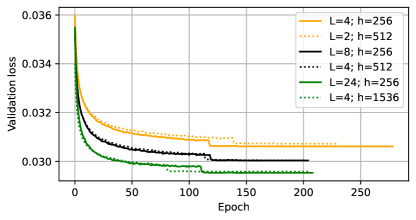
The number of trainable parameters scales linearly with both the number of residual blocks $L$ and the hidden dimension $h$ of the residual-MLPs, see Equation 1. Figure S1 plots the validation loss of different 8-bytes QINCo models trained on BigANN. Curves with the same color have the same model capacity, but differ in $L$ and $h$. It can be seen that changing one or the other has a similar effect on model performance. A slight advantage is visible for increasing $L$ rather than $h$. For that reason —in order to create only one parameter that influences model capacity— we propose to fix $h\!=\!256$ and adjust $L$ to change the capacity of QINCo.

Figure S1: Validation loss on 8 bytes encoding QINCo models trained on 10M BigANN. Changing the model capacity using either $L$ or $h$ with the same factor similarly affects validation loss.

B.2 Codeword usage

To investigate whether QINCo suffers from codebook collapse — a common problem in neural quantization models — one can use the average Shannon entropy (averaged over codebooks) to expresses the distribution of selected codewords by the compressed database. It is defined as:

$$\mathcal{H}=-\frac{1}{M}\sum_{m=1}^{M}\sum_{k=1}^{K}p^{m}_{k}\log_{2}(p^{m}_{k}),$$

and upper-bounded by $\log_{2}(K)$ bits. Here, $p^{m}_{k}$ is the empirical probability that the $k^{\text{th}}$ codeword gets assigned in the $m^{\text{th}}$ codebook when compressing the full database.

We find that QINCo achieves near-optimal codeword usage, $\mathcal{H}\approx\log_{2}(K)$ bits, in all cases, see Table S1. Note that UNQ (Morozov and Babenko, 2019) also achieves this, but it requires regularization at training time, which introduces an additional hyperparameter that weighs this regularizing term. Also the authors of DeepQ (Zhu et al., 2023) propose to use such a regularization term.

The fact that QINCo is not reliant on such additional regularization can be attributed to (i) QINCo is initialized with base codebooks using RQ that enforces a good inital spread of assignments, and (ii) since QINCo does not deploy an encoder before quantization, that encoder cannot cause codebook collapse by mapping all data vectors to a similar point in latent space.

		BigANN1M		Deep1M
8 bytes	OPQ		7.90		7.95
	RQ		7.95		7.96
	LSQ		7.95		7.95
	UNQ		8.00		7.99
	QINCo		7.99		7.99
16 bytes	OPQ		7.94		7.93
	RQ		7.97		7.98
	LSQ		7.93		7.94
	UNQ		7.99		7.99
	QINCo		7.99		7.99

Table S1: Entropy $\mathcal{H}$ of codeword assignments, averaged over codebooks, of the compressed database.

(a) MSE on BigANN1M

(b) R@1 on BigANN1M

(c) MSE on Deep1M

(d) R@1 on Deep1M

Figure S2: MSE and R@1 for BigANN1M and Deep1M for QINCo ($L=16$) trained for 8 byte and 16 byte encodings, truncated at a varying number of bytes.

Figure S3: Speed in queries per second (QPS) vs. accuracy (R@1) trade-offs for the Deep1B dataset.

B.3 Dynamic rates

Figure S2 shows the MSE and R@1 performance for QINCo trained for 8 bytes and 16 bytes encoding. We observe that QINCo trained for 8 and 16 bytes encoding performs very similar at the varying rates.

In Table S2 we recap the results of UNQ from Table 1 of the main paper using 16 byte encoding, and compare them to QINCo results using 12 and 13 byte encoding. The results of QINCo using 12 bytes equal or improve over those of UNQ using 16 bytes, except for MSE on Deep1M where we match UNQ 16 byte results with QINCo using 13 bytes.

		BigANN1M		Deep1M
	Code length	MSE	R@1	MSE	R@1
		($\times 10^{4}$)
UNQ	16 bytes	0.57	59.3	0.07	47.9
QINCo	12 bytes	0.57	61.8	0.08	49.7
QINCo	13 bytes	0.49	64.1	0.07	53.0

Table S2: Comparison of UNQ with 16 byte encoding, and QINCo with 12 and 13 byte encoding.

Figure S4: The set of parameters that are tried out for one of the curves of Figure 3. Each point is obtained by setting three parameters: the ${P_{\mathrm{IVF}}}$, HNSW’s efSearch and $n_{\mathrm{short}}$. We indicate the values of these parameters (in this order) for some of the results and color them from lowest (blue) to highest (red) with green in-between.

Figure S5: All combinations of ${P_{\mathrm{IVF}}}$ and $n_{\mathrm{short}}$ for one dataset. For some points we indicate the ${P_{\mathrm{IVF}}}$ value.

B.4 Fast search

Results on Deep1B. Figure S3 shows the speed-recall trade-offs for the Deep1B dataset, similar to the results shown for BigANN1B in Figure 3 of the main paper. There is a wide range of high-accuracy operating points where QINCo is competitive or outperforms IVF-PQ and IVF-RQ for 8 and 16 byte encoding. The trade-offs for the 32-byte setting are less interesting compared to RQ and PQ, because here the upper bound accuracy of QINCo w.r.t. these methods is not high enough. It is possible that PQ-QINCo would be a better option in this case.

Both for BigANN1B (Figure 3) and Deep1B (Figure S3), it can be seen that the capacity parameter $L$ slightly changes the Pareto front (green vs. yellow curves). At high accuracy operating points, IVF-QINCo with $L\!=\!2$ starts to become slower than IVF-QINCo with $L\!=\!4$, which seems counter-intuitive. This, however, is caused by the fact that in this regime, IVF-QINCo with $L\!=\!2$ requires a longer short-list (higher $n_{\mathrm{short}}$) than IVF-QINCo with $L\!=\!4$ to achieve the same accuracy, while at lower accuracies IVF-QINCo with $L\!=\!2$ is faster due to its lower decoding complexity.

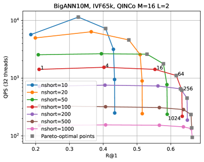
Decomposing performance over parameters. Pareto optimal curves do not show the runtime parameters that are used in each experiment. Figure S5 shows all the combination of parameters for a small experiment with 10M database elements and an IVF index of just $2^{16}=64$k centroids. In this case, the IVF centroids are searched exhaustively, without an approximate HNSW index, so there is no efSearch parameter involved. This makes it possible to show all parameter combinations. The Pareto-optimal points are indicated in gray squares: they are the ones that give the best accuracy for a given time budget or conversely the fastest search for a given recall requirement.

		BigANN1M						Deep1M
		MSE ($\times 10^{4}$)	R@1	R@10	R@100	no. params.		MSE	R@1	R@10	R@100	no. params.
		8 bytes
I	QINCo	1.40	39.7	87.4	99.6	4.2M		0.15	29.6	77.6	98.5	3.1M
II	QINCo only last loss $\mathcal{L}^{M}_{\text{{QINCo}}}(\theta)$	2.81	16.2	55.4	90.8	4.2M		0.20	17.4	55.8	91.6	3.1M
III	QINCo $M$ detached losses	1.42	39.1	87.6	99.5	4.2M		0.15	30.0	78.0	98.8	3.1M
IV	QINCo share concatenate blocks over $M$	1.46	38.8	87.5	99.5	4.0M		0.15	28.7	75.7	98.4	3.0M
V	QINCo share residual-MLPs over $M$	1.69	37.0	85.4	99.3	1.0M		0.16	27.4	74.5	98.1	0.7M
VI	QINCo share concatenate blocks & residual-MLPs	1.66	37.1	85.2	99.4	0.8M		0.16	28.4	75.4	97.9	0.6M
		16 bytes
I	QINCo	0.47	65.7	99.0	100.0	8.9M		0.06	53.2	96.6	100.0	6.6M
II	QINCo only last loss $\mathcal{L}^{M}_{\text{{QINCo}}}(\theta)$	2.85	16.1	53.2	90.1	8.9M		0.14	27.1	72.3	97.1	6.6M
III	QINCo $M$ detached losses	0.52	65.2	98.7	100.0	8.9M		0.06	53.1	96.5	100.0	6.6M
IV	QINCo share concatenate blocks over $M$	0.49	66.2	99.0	100.0	8.4M		0.07	51.4	95.7	100.0	6.3M
V	QINCo share residual-MLPs over $M$	0.69	61.8	98.5	100.0	1.5M		0.08	50.0	94.7	100.0	1.1M
VI	QINCo share concatenate blocks & residual-MLPs	0.71	59.4	98.3	100.0	1.1M		0.08	49.6	95.2	100.0	0.8M

Table S3: Ablation performance for QINCo models trained on $T=500$k vectors, with $L=8$. Compared to the base QINCo model (I), performance heavily degrades when using only the MSE loss on the last quantization step (II). Detaching the $M$ losses does slightly deteriorate the MSE reconstruction performance in all cases, but does not seem to affect recall that much (III). Sharing trainable parameters across the $M$ quantization steps reduces performance (IV-VI), mainly when a large part of the parameters are shared (VI).

Figure S4 show the same trade-offs for the BigANN1B dataset for a subset of the parameter sets. It shows that for Pareto-optimal points, the three considered parameters need to be set to “compatible” values: it is useless to set a high ${P_{\mathrm{IVF}}}$ with a low $n_{\mathrm{short}}$ and vice-versa. The granularity of the parameter we tried out is relatively coarse. The settings for ${P_{\mathrm{IVF}}}$ are clearly separated and there are probably slightly better operating points for intermediate settings like $n_{\mathrm{short}}=30$ or $n_{\mathrm{short}}=700$.

B.5 Ablations

Table S3 shows results of the ablations for which the main conclusions were provided in Section 5.4. Below we provide more details for each of those.

One loss vs. $\mathbf{M}$ losses. QINCo can be trained using only an MSE loss after the last quantization step, i.e. $\mathcal{L}^{M}_{\text{{QINCo}}}(\theta)$, instead of using the $M$ losses as given in Equation 3. In Table S3, however, we show that this drastically reduces performance. Additionally, we observed that optimization became more unstable, which could not be circumvented by using a lower (base) learning rate.

Training the $\bf M$ models separately. The $M$ losses in QINCo can be detached, such that each $m^{\text{th}}$ loss only updates the trainable parameters in the $m^{\text{th}}$ part of QINCo. Table S3 shows that MSE in all cases deteriorated, while the recall performances remained rather similar, or slightly increased for 8 bytes Deep1B encoding. In general, we might thus conclude that there is no large effect of the $m^{\text{th}}$ loss function on earlier quantization steps (i.e. $<m$). This corroborates the earlier-made observation that QINCo can be used with dynamic rates during evaluation.

Sharing parameters over quantization steps. The number of trainable parameters in QINCo scales linearly with $M$, the number of bytes used for quantization, see Equation 1. To test whether QINCo actually benefits from having $M$ specialized codebook-updating models, we share (a subset of the) parameters of each of those models over all $M$ steps. We run three variants: (i) only the parameters of the first concatenation block are shared, (ii) only the parameters of the residual-MLPs are shared, and (iii) both the concatenation block and residual-MLP parameters are shared over $M$. All models were trained on $T=500$k vectors, and with $L=8$ residual blocks. Table S3 shows that performance indeed drops when the codebook-predicting models are shared over the $M$ quantization steps. A direct relation is visible between the number of parameters that gets reduced by these actions, and the drop in performance. This finding suggests that the QINCo benefits from learning $M$ specialized codebook-predicting models.

		BigANN1M				Deep1M				Contriever1M				FB-ssnpp1M
	$T$	MSE ($\times 10^{4}$)	R@1	R@10	R@100	MSE	R@1	R@10	R@100	MSE	R@1	R@10	R@100	MSE ($\times 10^{4}$)	R@1	R@10	R@100
	8 bytes
OPQ	500k	2.95	21.9	64.8	95.4	0.26	15.9	51.2	88.2	1.87	8.0	24.7	50.8	9.52	2.5	5.1	10.9
OPQ	10M	2.99	21.3	64.3	95.6	0.26	15.1	51.1	87.9	1.87	8.5	24.3	50.4	9.52	2.5	5.0	11.2
RQ	500k	2.49	27.9	75.2	98.2	0.20	21.4	63.5	95.2	1.82	10.2	26.9	52.4	9.20	2.7	6.1	13.6
RQ	10M	2.49	27.9	75.2	98.0	0.20	21.9	64.0	95.2	1.82	9.7	27.1	52.6	9.18	2.7	5.9	14.3
LSQ	500k	1.91	31.9	79.5	98.9	0.17	24.6	69.4	97.0	1.65	13.1	33.9	62.7	8.87	3.3	7.5	17.3
LSQ	10M	1.89	30.6	78.7	98.9	0.17	24.5	68.8	96.7	1.64	13.1	34.9	62.5	8.82	3.5	8.0	18.2
UNQ	500k	1.51	34.6	82.8	99.0	0.16	26.7	72.6	97.3	—	—	—	—	—	—	—	—
UNQ∗	10M	1.12	39.7	88.3	99.6	0.14	29.2	77.5	98.8	—	—	—	—	—	—	—	—
QINCo	500k	1.38	40.2	88.0	99.6	0.15	29.4	77.6	98.5	1.57	15.4	38.0	65.5	8.95	3.0	7.7	17.1
QINCo	10M	1.12	45.2	91.2	99.7	0.12	36.3	84.6	99.4	1.40	20.7	47.4	74.6	8.67	3.6	8.9	20.6
	16 bytes
OPQ	500k	1.79	40.5	89.9	99.8	0.14	34.9	82.2	98.9	1.71	18.3	40.9	65.4	7.25	5.0	11.8	25.9
OPQ	10M	1.79	41.3	89.3	99.9	0.14	34.7	81.6	98.8	1.71	18.1	40.9	65.8	7.25	5.2	12.2	27.5
RQ	500k	1.30	49.0	95.0	100.0	0.10	43.0	90.8	99.8	1.65	20.2	43.5	68.2	7.01	5.4	13.0	29.0
RQ	10M	1.30	49.1	94.9	100.0	0.10	42.7	90.5	99.9	1.65	19.7	43.8	68.6	7.00	5.1	12.9	30.2
LSQ	500k	0.98	51.1	95.4	100.0	0.09	42.3	89.7	99.8	1.35	25.6	53.8	78.6	6.63	6.2	14.8	32.3
LSQ	10M	0.97	49.8	95.3	100.0	0.09	41.4	89.3	99.8	1.33	25.8	55.0	80.1	6.55	6.3	16.2	35.0
UNQ	500k	0.57	59.3	98.0	100.0	0.07	47.9	93.0	99.8	—	—	—	—	—	—	—	—
UNQ∗	10M	0.47	64.3	98.8	100.0	0.06	51.5	95.8	100.0	—	—	—	—	—	—	—	—
QINCo	500k	0.47	65.5	99.1	100.0	0.06	53.0	96.2	100.0	1.30	26.5	54.3	79.5	6.88	5.7	14.4	31.6
QINCo	10M	0.32	71.9	99.6	100.0	0.05	59.8	98.0	100.0	1.10	31.1	62.0	85.9	6.58	6.4	16.8	35.5

Table S4: Performance gain by scaling up from $T\!=\!500$k training vectors to $T\!=\!10$M vectors is limited for OPQ, RQ and LSQ, while QINCo improves further when more training data is available. Also UNQ improves from more training data, see Section B.6 for more details on scaleability of UNQ. Training on 500k vectors, QINCo is reported with the number of residual blocks $L$ that resulted in best performance. For both rates, this was $L\!=\!12$ for BigANN1M and Deep1M, $L\!=\!1$ for Contriever1M, and $L\!=\!2$ for Fb-ssnpp1M. When using 10M training vectors we report QINCo with $L\!=\!16$ in general, and $L\!=\!12$ for Contriever1M. For UNQ we report numbers from the original paper (Morozov and Babenko, 2019), where models were trained on 500k vectors, as well as the results of models we trained on 10M vectors using their codebase, denoted UNQ^∗. For the 8 byte setting, UNQ^∗ achieved highest performance using a hidden dimension of $h^{\prime}\!=\!1,536$ and $L^{\prime}\!=\!6$ encoder/decoder layers. For 16 bytes, best performance was found using $h^{\prime}\!=\!1,536$ and $L^{\prime}\!=\!4$.

B.6 Scaling baselines

Table S4 shows the performance for QINCo and all baselines both trained on 500k vectors and 10M vectors. OPQ, RQ and LSQ do not benefit from more training data in general, while UNQ did improve. A more detailed analysis on UNQ’s scalability follows in this section.

In Table S4, for 500k training vectors we use the original numbers from the paper (Morozov and Babenko, 2019), while we denote with UNQ^∗ results we obtained by training on 10M vectors by re-running the author’s codebase, while model selection was based on the hold-out validation set that we created, see Section A.2. The triplet loss was not used in this scenario as the negative mining on 10M training vectors resulted in prohibitively slow training.

On 500k training vectors, we found that any increase in model size led to overfitting and increasing MSE numbers. However, we did find that UNQ scaled to 10M training vectors quite well for both BigANN1M and Deep1M, with R@1 numbers improving from 34.6% to 39.7% and from 26.7% to 29.2% on Deep1M, respectively for 8 bytes. Similar results are observed for 16 bytes. Despite this, from Figure S6 we see that QINCo scales even better; MSE rapidly decreases with increasing capacity with far fewer parameters, for both quantities of training data. This shows that QINCo outperforms UNQ both in the low- and high-data regime (with capacity being scaled accordingly).

Note that we experimented with changing the depth $L^{\prime}$ of the encoder and decoder of UNQ. This parameter was fixed to $L^{\prime}=2$ by the authors, and therefore we did not parameterize $L^{\prime}$ in Tab. 3. Including $L^{\prime}$ in the number of FLOPS for encoding and decoding of UNQ, results in $h^{\prime}\big{(}D\!+\!(L^{\prime}-1)h^{\prime}\!+\!Mb\!+\!MK\big{)}$ and $h^{\prime}\big{(}b\!+\!(L^{\prime}-1)h^{\prime}\!+\!D\!+\!M\big{)}$, respectively.

Figure S6: Scaling results comparing UNQ to QINCo. All UNQ models were trained by us using the author’s code. For the UNQ training with $T\!=\!500$k vectors, all increases in parameter counts based on expanding the encoder/decoder led to overfitting, and so we observed optimal model performance with hyperparameters from the paper. The single point visualized for “UNQ, 500k” in both graphs is close to the MSE of the models presented by Morozov and Babenko (2019), but with the model selection criteria outlined in Section A.2. For $T\!=\!10$M vectors, we found the best UNQ model used a hidden dimension of $h^{\prime}\!=\!1,536$ (instead of the default 1,024), and so in our plots we scale the number of layers in the encoder and decoder using $L^{\prime}\in\{2,4,6\}$. Note that these Pareto curves include the optimal performance point for UNQ reported in Table S4. For QINCo we show curves with $h\!=\!256$ and $L\in\{2,4,8,12,16\}$. With all settings, UNQ has worse operating points for both model and data scaling than QINCo. In some cases, stability was an issue, as can be seen for the highest parameter count setting with UNQ for the 16 byte results.

References

- Agustsson et al. (2017) Eirikur Agustsson, Fabian Mentzer, Michael Tschannen, Lukas Cavigelli, Luca Benini, and Luc Van Gool. Soft-to-hard vector quantization for end-to-end learning compressible representations. In NeurIPS, 2017.
- Amara et al. (2022) Kenza Amara, Matthijs Douze, Alexandre Sablayrolles, and Hervé Jégou. Nearest neighbor search with compact codes: A decoder perspective. In ICMR, 2022.
- Babenko and Lempitsky (2014) Artem Babenko and Victor Lempitsky. Additive quantization for extreme vector compression. In CVPR, 2014.
- Babenko and Lempitsky (2015) Artem Babenko and Victor Lempitsky. Tree quantization for large-scale similarity search and classification. In CVPR, 2015.
- Babenko and Lempitsky (2016) Artem Babenko and Victor Lempitsky. Efficient indexing of billion-scale datasets of deep descriptors. In CVPR, 2016.
- Baranchuk et al. (2018) Dmitry Baranchuk, Artem Babenko, and Yury Malkov. Revisiting the inverted indices for billion-scale approximate nearest neighbors. In ECCV, 2018.
- Chang et al. (2022) Huiwen Chang, Han Zhang, Lu Jiang, Ce Liu, and William T. Freeman. MaskGIT: Masked generative image transformer. In CVPR, 2022.
- Chen et al. (2010) Yongjian Chen, Tao Guan, and Cheng Wang. Approximate nearest neighbor search by residual vector quantization. Sensors, 10(12):11259–11273, 2010.
- Copet et al. (2023) Jade Copet, Felix Kreuk, Itai Gat, Tal Remez, David Kant, Gabriel Synnaeve, Yossi Adi, and Alexandre Défossez. Simple and controllable music generation. arXiv preprint, 2306.05284, 2023.
- Cover and Thomas (1991) Thomas M Cover and Joy A Thomas. Elements of Information Theory. John Wiley & Sons, 1991.
- Défossez et al. (2023) Alexandre Défossez, Jade Copet, Gabriel Synnaeve, and Yossi Adi. High fidelity neural audio compression. Transactions on Machine Learning Research, 2023.
- Devlin et al. (2018) Jacob Devlin, Ming-Wei Chang, Kenton Lee, and Kristina Toutanova. BERT: Pre-training of deep bidirectional transformers for language understanding. arXiv preprint, 1810.04805, 2018.
- Douze et al. (2016) Matthijs Douze, Hervé Jégou, and Florent Perronnin. Polysemous codes. In ECCV, 2016.
- Douze et al. (2024) Matthijs Douze, Alexandr Guzhva, Chengqi Deng, Jeff Johnson, Gergely Szilvasy, Pierre-Emmanuel Mazaré, Maria Lomeli, Lucas Hosseini, and Hervé Jégou. The faiss library. arXiv preprint arXiv:2401.08281, 2024.
- El-Nouby et al. (2023) Alaaeldin El-Nouby, Matthew J Muckley, Karen Ullrich, Ivan Laptev, Jakob Verbeek, and Hervé Jégou. Image compression with product quantized masked image modeling. Transactions on Machine Learning Research, 2023.
- Esser et al. (2021) Patrick Esser, Robin Rombach, and Bjorn Ommer. Taming transformers for high-resolution image synthesis. In CVPR, 2021.
- Ge et al. (2013) Tiezheng Ge, Kaiming He, Qifa Ke, and Jian Sun. Optimized product quantization for approximate nearest neighbor search. In CVPR, 2013.
- Glynn (1990) Peter W. Glynn. Likelihood ratio gradient estimation for stochastic systems. Communications of the ACM, 33(10):75–84, 1990.
- Gray (1984) Robert Gray. Vector quantization. Transactions on Acoustics, Speech and Signal Processing, 1(2):4–29, 1984.
- Guo et al. (2020) Ruiqi Guo, Philip Sun, Erik Lindgren, Quan Geng, David Simcha, Felix Chern, and Sanjiv Kumar. Accelerating large-scale inference with anisotropic vector quantization. In ICML, 2020.
- He et al. (2013) Kaiming He, Fang Wen, and Jian Sun. K-means hashing: An affinity-preserving quantization method for learning binary compact codes. In CVPR, 2013.
- He et al. (2016) Kaiming He, Xiangyu Zhang, Shaoqing Ren, and Jian Sun. Deep residual learning for image recognition. In CVPR, 2016.
- Huh et al. (2023) Minyoung Huh, Brian Cheung, Pulkit Agrawal, and Phillip Isola. Straightening out the straight-through estimator: Overcoming optimization challenges in vector quantized networks. In ICML, 2023.
- Huijben et al. (2022) Iris AM Huijben, Wouter Kool, Max B Paulus, and Ruud JG Van Sloun. A review of the gumbel-max trick and its extensions for discrete stochasticity in machine learning. Transactions on Pattern Analysis and Machine Intelligence, 45(2):1353–1371, 2022.
- Izacard et al. (2022) Gautier Izacard, Mathilde Caron, Lucas Hosseini, Sebastian Riedel, Piotr Bojanowski, Armand Joulin, and Edouard Grave. Unsupervised dense information retrieval with contrastive learning. Transactions on Machine Learning Research, 2022.
- Jang et al. (2017) Eric Jang, Shixiang Gu, and Ben Poole. Categorical reparameterization with Gumbel-Softmax. In ICLR, 2017.
- Jégou et al. (2010) Hervé Jégou, Matthijs Douze, and Cordelia Schmid. Product quantization for nearest neighbor search. Transactions on Pattern Analysis and Machine Intelligence, 33(1):117–128, 2010.
- Jégou et al. (2011) Hervé Jégou, Romain Tavenard, Matthijs Douze, and Laurent Amsaleg. Searching in one billion vectors: Re-rank with source coding. In ICASSP, 2011.
- Kingma and Ba (2015) Diederik P. Kingma and Jimmy Ba. Adam: A method for stochastic optimization. In ICLR, 2015.
- Klein and Wolf (2019) Benjamin Klein and Lior Wolf. End-to-end supervised product quantization for image search and retrieval. In CVPR, 2019.
- Kumar et al. (2023) Rithesh Kumar, Prem Seetharaman, Alejandro Luebs, Ishaan Kumar, and Kundan Kumar. High-fidelity audio compression with improved RVQGA. arXiv preprint, 2306.06546, 2023.
- Lee et al. (2022) Doyup Lee, Chiheon Kim, Saehoon Kim, Minsu Cho, and Wook-Shin Han. Autoregressive image generation using residual quantization. In CVPR, 2022.
- Maddison et al. (2017) Chris J. Maddison, Andriy Mnih, and Yee Whye Teh. The concrete distribution: A continuous relaxation of discrete random variables. In ICLR, 2017.
- Malkov and Yashunin (2018) Yu A. Malkov and Dmitry A. Yashunin. Efficient and robust approximate nearest neighbor search using hierarchical navigable small world graphs. Transactions on Pattern Analysis and Machine Intelligence, 42(4):824–836, 2018.
- Martinez et al. (2016) Julieta Martinez, Joris Clement, Holger H Hoos, and James J Little. Revisiting additive quantization. In ECCV, 2016.
- Martinez et al. (2018) Julieta Martinez, Shobhit Zakhmi, Holger H Hoos, and James J Little. LSQ++: Lower running time and higher recall in multi-codebook quantization. In ECCV, 2018.
- Morozov and Babenko (2019) Stanislav Morozov and Artem Babenko. Unsupervised neural quantization for compressed-domain similarity search. In ICCV, 2019.
- Niu et al. (2023) Lushuai Niu, Zhi Xu, Longyang Zhao, Daojing He, Jianqiu Ji, Xiaoli Yuan, and Mian Xue. Residual vector product quantization for approximate nearest neighbor search. Expert Systems with Applications, 232, 2023.
- Oquab et al. (2023) Maxime Oquab, Timothée Darcet, Théo Moutakanni, Huy Vo, Marc Szafraniec, Vasil Khalidov, Pierre Fernandez, Daniel Haziza, Francisco Massa, Alaaeldin El-Nouby, et al. Dinov2: Learning Robust Visual Features Without Supervision. arXiv preprint arXiv:2304.07193, 2023.
- Paterek (2007) Arkadiusz Paterek. Improving regularized singular value decomposition for collaborative filtering. In Proceedings of KDD cup and workshop, 2007.
- Pizzi et al. (2022) Ed Pizzi, Sreya Dutta Roy, Sugosh Nagavara Ravindra, Priya Goyal, and Matthijs Douze. A self-supervised descriptor for image copy detection. In CVPR, 2022.
- Radford et al. (2021) Alec Radford, Jong Wook Kim, Chris Hallacy, Aditya Ramesh, Gabriel Goh, Sandhini Agarwal, Girish Sastry, Amanda Askell, Pamela Mishkin, Jack Clark, Gretchen Krueger, and Ilya Sutskever. Learning transferable visual models from natural language supervision. In ICML, 2021.
- Schwenk and Douze (2017) Holger Schwenk and Matthijs Douze. Learning joint multilingual sentence representations with neural machine translation. In Workshop on Representation Learning for NLP, 2017.
- Simhadri et al. (2022) Harsha Vardhan Simhadri, George Williams, Martin Aumüller, Matthijs Douze, Artem Babenko, Dmitry Baranchuk, Qi Chen, Lucas Hosseini, Ravishankar Krishnaswamny, Gopal Srinivasa, et al. Results of the NeurIPS’21 challenge on billion-scale approximate nearest neighbor search. In NeurIPS 2021 Competitions and Demonstrations Track, 2022.
- Subramanya et al. (2019) Suhas Jayaram Subramanya, Rohan Kadekodi, Ravishankar Krishaswamy, and Harsha Vardhan Simhadri. DiskANN: Fast accurate billion-point nearest neighbor search on a single node. In NeurIPS, 2019.
- van den Oord et al. (2017) Aaron van den Oord, Oriol Vinyals, and Koray Kavukcuoglu. Neural discrete representation learning. In NeurIPS, 2017.
- Williams (1992) Ronald J. Williams. Simple statistical gradient-following algorithms for connectionist reinforcement learning. Machine learning, 8(3):229–256, 1992.
- Ypsilantis et al. (2023) Nikolaos-Antonios Ypsilantis, Kaifeng Chen, Bingyi Cao, Mário Lipovskỳ, Pelin Dogan-Schönberger, Grzegorz Makosa, Boris Bluntschli, Mojtaba Seyedhosseini, Ondřej Chum, and André Araujo. Towards universal image embeddings: A large-scale dataset and challenge for generic image representations. In ICCV, 2023.
- Zhu et al. (2023) Xiaosu Zhu, Jingkuan Song, Lianli Gao, Xiaoyan Gu, and Heng Tao Shen. Revisiting multi-codebook quantization. Transactions on Image Processing, 32:2399–2412, 2023.