A deep neural network physics-based reduced order model for dynamic stall

Abstract

Dynamic stall is a challenging fluid dynamics phenomenon occurring during rapid transient motion of airfoils where the angle of attack exceeds the static stall angle. Understanding dynamic stall is essential for designing efficient aerodynamic systems in applications such as helicopters, wind turbines, and specific aircraft maneuvers. The highly non-linear unsteady aerodynamic phenomena involved in dynamic stall are challenging to be included in a reduced order model. In this work, a physics-based machine learning framework is developed to fast predict the aerodynamic forces and momentum for a pitching NACA0012 airfoil incurring in light and deep dynamic stall. Three deep neural network architectures of increasing complexity are investigated, ranging from two multilayer perceptrons to a convolutional neural network. The proposed model is able to robustly predict pressure and skin friction distributions over the airfoil for an entire pitching cycle. Periodic conditions are implemented to grant the physical smoothness of the solution both in space and time. Furthermore, an improved loss function incorporating physical knowledge to compute the airfoil loads is presented. An analysis of the dataset point distributions to cover the flight envelope is performed highlighting the effects of adopting low discrepancy sequences, like Latin hypercube, Sobol’, and Halton, compared to random and uniform grid ones. The current model shows unprecedented performances in predicting forces and momentum in a broad range of flight conditions.

I Introduction

Dynamic stall is a highly nonlinear unsteady aerodynamic phenomenon generated by large angles of attack in combination with rapid variations of incidence. Dynamic stall can be encountered in a wide range of aeronautical applications, i.e., blades of helicopter rotors, wind turbines, turbo-machinery and maneuvering fixed wing aircraft. The ability to predict and mitigate dynamic stall results in an improvement of safety standards and also a better estimation of the flight envelopes [1]. Compared to static stall, dynamic stall develops at a larger effective angle due to the rapid increase of incidence that temporary delays the boundary layer separation. The delay in the boundary layer separation is attributed to two effects. One is an increase in the effective camber that is predicted by quasi-steady thin airfoil theory. The other is the acceleration of the boundary layer due to the Magnus effect produced by the motion of the leading edge [2]. The boundary layer separation is followed by a large flow detachment on the suction side of the profile. This results in a disrupt loss of lift, a strong pitch down moment, and an increase in drag. Before the flow reattachment, the profile underlays varying loads due to the chaotic nature of the involved phenomena [3]. The variation of the effective angle of attack can be generated by a blade pitch, like in helicopter blades, or due to a change in the relative flow velocity, as in gust encounters [4, 2].

Many experiments and computational simulations have been performed to investigate dynamic stall phenomena and study the flow around pitching and plunging airfoils [5, 6]. Especially during the last decade, thanks to the advances in numerical methods and computational power provided by modern GPGPUs [7, 8] together with optical measurements techniques [9, 10, 11], dynamic stall has received particular attention in the literature where considerable advances in modeling, prediction, and understanding are reported. State-of-the-art numerical simulations consist in wall-resolved large eddy simulations (LES) of ramp-up motion for spanwise-extruded airfoils [12, 13]. Several aspects of dynamic stall have been numerically investigated ranging from aspect ratio [14, 15] to sweep angle [16] and compressibility effects [17].

One aspect, crucial in many practical applications, is the formulation of a reduced order model (ROM) for dynamic stall. The two most common models nowadays are Leishman-Beddoes and ONERA ones. Beddoes model was originally developed in the 1970s in indicial formulation [18, 19]. After, some improvements have been included and it became the well-known Leishman-Beddoes model [20, 21, 22]. In order to include it in aeroelastic codes, also a state-space representation is available in the literature [23, 24]. The latest version of the Leismann-Beddoes model is reported in Beddoes [25] and it is known as “Third Generation Model” that improves the predicted loads for low Mach numbers and low reduced frequencies adding two equations with respect to the previous generation model. The ONERA model describes the unsteady airfoil behavior using a set of nonlinear differential equations, attempting to predict the response in the time domain [26, 27]. In contrast to Leishman-Beddoes one, the ONERA formulation does not include physics involved in dynamic stall but it only tries to describe the hysteresis effects. In Truong [28, 29] the latest version, called “ONERA BH model”, is presented.

Recent developments in dynamic stall ROM try to leverage high-fidelity numerical simulations to better understand the phenomena and gather data from larger datasets. The two most common algebraic methods present in literature, to extract spatio-temporal flow features, are Proper Orthogonal Decomposition (POD) [30] and Dynamic Mode Decompositions (DMD) [31, 32]. An example of a dynamic stall ROM, which leverage Spectral Proper Orthogonal Decomposition (SPOD) to decompose the velocity flow field from a Delayed Detached Eddy Simulations (DDES) with SST model, has been developed in Avanzi et al. [33, 34]. The works define an appropriate operating range of the filter’s typical dimension to further investigate coherent structures in the process and tries to reconstruct force and momentum coefficients over the pitching cycle using a reduced set of modes. Another recent extensive work in the same direction is presented in Chiu et al. [35], where large eddy simulations (LES) with SPOD are adopted to analyze the impact of coherent structures on the aerodynamic forces. The authors discovered that the zeroth frequency of the first mode is linked to an oscillating near-wall stream that adheres to the reattachment flow pattern. Subsequently, the first frequency is associated with a pair of counter-rotating vortices emerging at the point of flow reattachment. Finally, the second frequency of the first mode corresponds to smaller counter-rotating vortex pairs at the shear layer, originating in close proximity to the reattachment point. In  Taha et al. [36] and Olea et al. [37], an extension of the classical airfoil theory to high angles of attack is presented. The model is designed to capture unsteady nonlinear characteristics at high angles of attack, and to conveniently apply nonlinear system analysis tools such as geometric-control theory and averaging. Tatar and Sabour [38] derived a nonlinear reduced model of the dynamic stall using a fuzzy inference system (FIS) and the adaptive network-based FIS (ANFIS). Furthermore, the Gram–Schmidt orthogonalization technique is used to construct a more complex structure of the input variables. The proposed reduced-order model is able to properly predict the aerodynamic response of the pitching airfoil at two reduced frequencies. Glaz et al. [39] describes a surrogate-based recurrence framework approach based on non-stationary Gaussian process models as a promising alternative to widely used semi-empirical rotorcraft dynamic stall models.

Another powerful tool that is becoming more and more popular in engineering applications is machine learning. Recent developments in deep learning bring advanced and innovative approaches to improve the efficiency, flexibility, and accuracy of the predictive models [40, 41]. Some of the outstanding applications of deep neural networks (DNNs) in the domain of computational physics are solution of partial differential equations (PDEs), like Physics-Informed Neural Networks (PINNs) [42, 43, 44, 45, 46]. Other neural network architectures that allow to analyze information from large datasets are Convolutional Neural Networks (CNNs). They received increasing attention by the fluid-mechanics community for their ability in pattern recognition [47, 48]. In addition, convolution layers are usually coupled with pooling and up-sampling layers, allowing to reduce or increase data size, respectively. The neural network capability of analyzing a large dataset has been of particular interest in dynamic stall phenomena since time-dependent series can be analyzed as a whole. In Lennie et al. [49], a clustering method based on dynamic time warping is used to find different shedding behaviors in experiments. The work analyses cycle-to-cycle variations and how to detect outliers of separated flows. A convolutional neural network is used to extract dynamic stall vorticity convection speeds and phases from pressure data. The method captures the fact that secondary and tertiary vorticity vary strongly, and in static stall with surging flow the flow can occasionally reattach. Another example of machine learning applied to dynamic stall can be found in Kasmaiee et al. [50]. A multi-layer perceptrons (MLP) neural networks is used to train the aerodynamic coefficients as functions of the control parameters and reduce the number of simulations. A genetic algorithm is employed to optimize the configuration of a pure suction jet actuator on an oscillating airfoil.  Damiola et al. [51] proposed a State-Space Neural Network (SS-NN) model trained using swept sines at several angle-of-attack ranges. The study shows that SS-NN can be a powerful tool to accurately predict the unsteady aerodynamic loads of a pitching airfoil, both in pre-stall and post-stall conditions. In particular, the model succeeds in correctly capturing highly nonlinear flow features such as the delay in flow separation, and the formation and shedding of the dynamic stall vortex. A final example is presented in Eivazi et al. [52], where an autoencoder network is used for non-linear dimension reduction and feature extraction as an alternative to singular value decomposition (SVD). Then, the extracted features are used as an input for a long short-term memory (LSTM) network to predict the velocity field at future time instances. A further confirmation of NN capabilities is given comparing with non-intrusive reduced order models based on dynamic mode decomposition and proper orthogonal decomposition [53, 54].

This work unveils a deep neural network-based framework designed to predict force and momentum coefficients throughout an entire pitching cycle, encompassing both light and deep dynamic stall conditions. The primary goal is to set a reduce order model that can rapidly predict the aerodynamic loads for the integration into an aeroelastic code. The flight envelope is defined by three parameters: the amplitude of the pitching angle $\alpha_{s}$, the reduced frequency $k$, and the free-stream velocity $V_{\infty}$. In section II, the dataset point sequences are explained with the numerical setup of computational fluid dynamics simulations to generate the datasets. Then, in section III, the three neural network architectures are presented together with the physics-based loss function. After describing the whole setup, the performances of the model are investigated in detail in the section  IV, highlighting the pros and cons. Finally, section V states the conclusions and the final remarks.

II Dataset generation

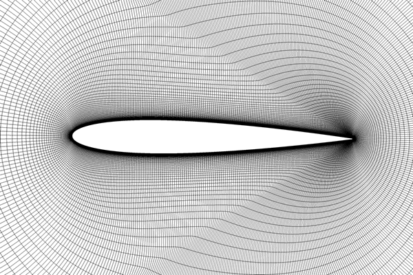
The dataset generation is based on the solution of the unsteady 2D RANS equations. The numerical setup starts from the comparison with the experimental campaign presented in Lee and Gerontakos [55]. A detailed grid convergence analysis and a study of the effects of the turbulence model is reported in Baldan and Guardone [56]. The main settings of the reference test case are summarized in the following for completeness. A NACA 0012 profile with 0.15 m chord underlying a sinusoidal pitching motion, at reduced frequency k = 0.1 and Reynolds number Re = $1.35\cdot 10^{5}$, is investigated. The free-stream velocity is $V_{\infty}$ = 14 m/s with a turbulent intensity equal to 0.08%, pressure is $P_{\infty}$ = 1 atm, and the pitching frequency $\omega$ is set equal to 18.67 Hz. The mean angle of attach $\alpha_{0}$ is equal to $10^{\circ}$, while the angle oscillation amplitude $\alpha_{s}$ is $15^{\circ}$. The medium O-grid mesh has been used in the computations, corresponding to 512 nodes over the profile and 128 nodes in the normal direction. The element size at the leading edge is equal to $2.0\cdot 10^{-3}\ \text{c}$ while at the trailing edge is $5.0\cdot 10^{-4}\ \text{c}$ according to best practice. The $y^{+}<1$ requirement is always satisfied at the wall, even for the most demanding simulation. In Figure 1, a detail of the mesh is reported. Numerical simulations are performed using ANSYS Fluent 2023R2. The unsteady incompressible RANS equations are solved using second-order upwind discretization and second-order implicit time integration scheme. Gradients are retrieved through a least square cell-based method, and fluxes are obtained with the Rhie-Chow momentum-based formulation. Pressure-velocity equations are solved using the SIMPLE method. A rigid motion of the entire grid is prescribed through a user-defined expression to allow the airfoil pitching, $\alpha(t)=\alpha_{0}+\alpha_{s}\sin(\omega t)$. The SST model with the intermittency equation [57] is employed to close the RANS equations. Each cycle is discretized with 3600 time steps. All the simulations are evolved until time convergence is reached between subsequent cycles, meaning that the obtained solution overlaps.

Figure 1: O-grid detail used in the computations.

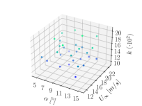
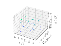
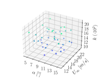
The flight envelope is defined by three variables to limit the dimensionality of the problem and reduce the number of performed simulations without compromising the applicability of the proposed framework. The input parameters of the model are the free-stream velocity $V_{\infty}$ that can vary between 12 and 22 m/s, the pitching amplitude angle $\alpha$ that ranges from $5^{\circ}$ to $15^{\circ}$, and the reduced frequency $k$ extends from 0.1 to 0.2. All the other parameters are kept equal to the reference test case. As a first train distribution, a uniform grid has been used to cover the input space utilizing 6 points in each dimension, namely 216 points in total. The test distributions, instead, are obtained through random sequences of 40 and 100 points and are adopted to evaluate the performances of the model in the following. Due to the poor performance of the uniform grid distribution for training, low discrepancy sequences have been used. Low-discrepancy distributions, also called quasi-random sequences, are sequences of points strategically generated to achieve a more uniform coverage of a space compared to purely random sequences. The objective is to minimize discrepancies or irregularities in the distribution of points, especially in higher dimensions. Unlike truly random sequences, low-discrepancy sequences, systematically distribute points across different dimensions to create a more even sampling of the input space. This regular and deterministic pattern is advantageous in numerical methods and simulations where a more uniform sampling contributes to improved accuracy. In detail Sobol’, Latin hypercube, and Halton sequences [58] are used for training with different sizes: 30, 40, 50, 100 and 216. The discrepancy of each distribution is reported in  1. A graphical representation of all the employed datasets can be found in Figure 2. Train datasets are reported in blue-green gradient while test datasets are in cyan-pink gradient.

Table 1: Discrepancy for Latin hypercube, Sobol’, and Halton sequences of the datasets in the unitary hypercube before scaling to real values.

Dataset size	Latin	Sobol’	Halton
30	5.18E-03	3.00E-03	2.44E-03
40	2.04E-03	1.52E-03	1.42E-03
50	2.70E-03	1.07E-03	1.25E-03
100	7.11E-04	3.36E-04	2.67E-04
216	2.52E-04	8.49E-05	8.02E-05

(a)

(b)

(c)

(d)

(e)

(f)

(g)

(h)

(i)

(j)

(k)

(l)

(m)

(n)

(o)

(p)

(q)

(r)

Figure 2: Sobol, Latin Hypercube, Halton, random, and uniform grid point datasets. Train datasets are represented in blue-green gradient while test datasets in cyan-pink gradient

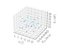
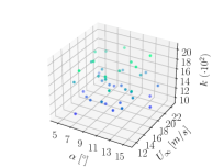
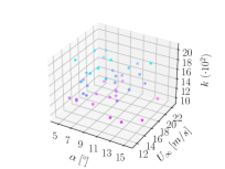
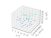
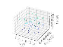
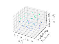
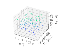
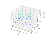
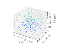
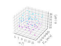
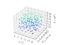
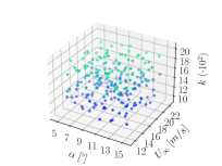
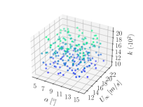
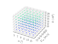
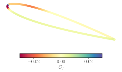
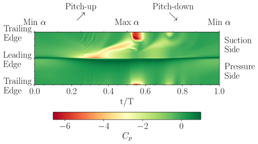
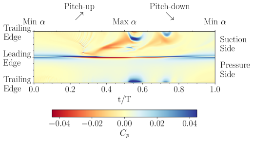
The outputs of each simulation, which populates the datasets, are the pressure coefficient and the skin friction coefficient distributions over the profile for each time step in one pitching cycle. The unstructured output from Fluent is mapped to the structured airfoil mesh using a k-d tree to search the nearest neighbors [59]. This allows to organize the output in a 3-dimensional array and to have comparable results for different simulations. The first direction corresponds to the time step and ranges from 1 to 3600. The second direction represents the airfoil surface coordinate. From 1 to 256 contains the data over the suction side of the profile while, from 257 to 512 refers to the pressure side. The last direction is equal to 2 and stores the physical data, namely $C_{p}$ and $C_{f}$. When the full dataset is considered, an additional dimension is present that identify the simulation index. The post-processed value of the skin friction in each point is equal to the signed magnitude. The sign is set according to the direction computed from the $x$ and $y$ components of the $C_{f}$. The positive geometric direction is defined as the curvilinear coordinate that goes from the leading edge to the trailing edge for both sides of the airfoil. An example is available in Figure 3. If the geometric direction and the $C_{f}$ direction computed from the numerical simulations coincide, the sign is positive otherwise, if they are opposite the sign is negative. This allows to highlight the regions where the flow is detached and helps the neural networks to identify stalled portions. Two aspects that can be noted in Figure 4 are the discontinuity at the leading edge due to the origin of the coordinate system and the recirculation portion on the suction side of the profile due to the backward advection of the dynamic stall vortex. Finally, in Figure 5, an example of spatio-temporal contour of the post-processed ${C_{p}}$ and ${C_{f}}$ distributions over an entire pitching cycle is available, highlighting the pitch-up and pitch-down phases and how the profile is mapped in the structured array.

Figure 3: Example of the curvilinear coordinate employed in the $C_{f}$ computation. The origin is located at the leading edge while the end is posed in the middle of the trailing edge for both sides of the airfoil.

Figure 4: Example of the post-processed ${C_{f}}$ distribution. It is noticeable the discontinuity at the leading edge due to the origin of the coordinate system and the recirculation portion on the suction side of the profile due to the backward advection of the dynamic stall vortex.

(a)

(b)

Figure 5: Example of spatio-temporal contour of the post-processed ${C_{p}}$ and ${C_{f}}$ distributions over an entire pitching cycle.

III Neural network architectures

(a)

(b)

(c)

(d)

Figure 6: Neural network architecture representations. Input parameters are: ${\alpha}$ angle oscillation amplitude, ${k}$ reduced pitching frequency, and ${V_{\infty}}$ free-stream velocity. When present, ${t}$ represents the time instant over the pitching period.

A multilayer perceptron (MLP) is a common name to identify feed-forward artificial neural network, consisting of fully connected neurons with a non-linear activation function, having at least three layers [60]. A convolutional neural network (CNN), instead, is a regularized type of feed-forward neural network that learns to optimize the filters, or kernels, through automated learning, whereas in traditional algorithms these filters are hand-engineered [61].

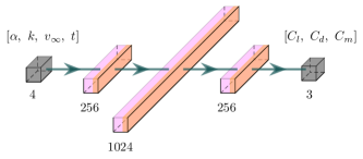
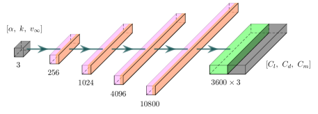
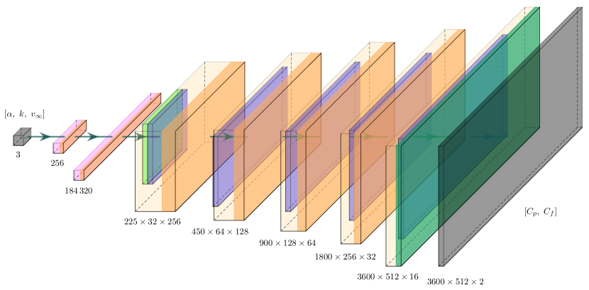
Three different neural network architectures are used in this work. The first two are MLPs, and a schematic representation is reported in Figures LABEL:img_mlp_single and LABEL:img_mlp_all. The third one is a CNN and is schematized in Figure LABEL:img_cnn. The level of complexity increases moving from the first to the last one. The flight condition inputs for all architectures correspond to three parameters, namely $\alpha$, $V_{\infty}$, and $k$, that are adimensionalized in the range $[0,1]$ using the minimum and maximum values of the flight envelope. An additional input $t$ is present in the first architecture that corresponds to the temporal instant over the pitching cycle. It is adimensionalized using the oscillation period, meaning that it can only assume the values in the well-known range $[0,1]$. The output is different for all architectures. In the first one, $C_{l}$, $C_{d}$, and $C_{m}$ at the inquired time instant are predicted. Moving to the next architecture, the same coefficients are computed but for the entire cycle leading to an output array of size $3600\times 3$. Finally, in the CNN the output corresponds to the pressure and skin friction distributions over the airfoil for all time steps of size $3600\times 512\times 2$. Starting from the output distributions, the force and momentum coefficients are straightforwardly retrieved from the airfoil geometry.

The simplest implementation, corresponding to the first architecture, consists in an MLP neural network that predicts $C_{l}$, $C_{d}$, and $C_{m}$ for a given flight condition and one temporal instant. For this reason, in the following is referred as “MLP Single”. It is characterized by three hidden layers of size 256, 1024, and 256 respectively. The activation function is Leaky ReLU (Rectified Linear Unit) which is commonly used to introduce non-linearity [62]. The Leaky ReLU activation function allows a small, positive gradient when the input is negative, helping to address the vanishing gradient problem. Mathematically, Leaky ReLU is defined as $f(x)=\max(\gamma x,x)$, where $\gamma$ is set equal to 0.1.

Moving to the second neural network, the structure is quite similar to the previous one since it always presents three hidden layers and adopts the same activation function. The differences underlay in the layer sizes that are: 256, 1024, and 4096. The last layer has size 10800 that is reshaped to $3600\times 3$ to cope with the output size. Due to the capability of predicting all the coefficients over one cycle is called “MLP All” for brevity.

Lastly, the Convolutional Neural Network is considered. The first two hidden layers are formed by fully connected and Leaky ReLU-activated of size 256 and 184 320. After, it is reshaped to $45\times 16\times 256$. The first up-sampling layer increases the first direction by a factor of 5 while the second direction is doubled, leading to the first convolution layer with leaky ReLU activation. Four up-sampling and convolution layers follows, where the feature dimension is halved, and the other two directions are doubled until the output size is reached. The last convolution layer that reduces the 16 features to the pressure and friction distributions has a linear activation. In the actual implementation, before each convolution, an additional ad-hoc implemented layer is computed to enlarge the data and ensure periodicity. This aspect is crucial from a physical point of view because it imposes that there are no discontinuities over the airfoil and also that the start and the end of two cycles are coincident. In TensorFlow, the convolution layers are applied to the extended data with padding equal to “valid”. This is the first difference with respect to the other two architectures that are not able to grant a physical meaning to the predicted data. Another advantage of having the $C_{p}$ and the $C_{f}$ distributions is the ability to compute the momentum coefficient with respect to an arbitrary point in the space that is not possible when directly learning the quarter-chord value.

The loss function $\mathcal{L}$ is the same in all the three architectures and it is the mean squared error (MSE).

$$\text{MSE}=\frac{1}{N}\sum_{i=1}^{N}(\hat{y}_{i}-y_{i})^{2}$$ (1)

Where $N$ is the number of data points, $\hat{y}_{i}$ is the predicted value for the $i$-th data point, and $y_{i}$ is the actual ground truth value for the $i$-th data point.

For the CNN, an additional loss function has been implemented and tested trying to incorporate more physical information in the model. The objective is to include the mean squared force and momentum coefficient error $\text{MSE}_{\text{C}_{\text{l}},\text{C}_{\text{d}},\text{C}_{\text{m}}}$ in the loss function $\mathcal{L}$ in addition to the MSE presented before $\text{MSE}_{\text{C}_{\text{p}},\text{C}_{\text{f}}}$.

$$\mathcal{L}=\text{MSE}_{\text{C}_{\text{p}},\text{C}_{\text{f}}}+\beta\cdot\text{MSE}_{\text{C}_{\text{l}},\text{C}_{\text{d}},\text{C}_{\text{m}}}$$ (2)

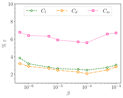
The hyperparameter $\beta$ controls the influence of the coefficient error in the total loss. The optimal value for $\beta$ has found to be equal to $1\cdot 10^{-4}$ in order to have a comparable error from the two contributions to the total loss function. A complete analysis on the influence of $\beta$ is reported in Figure 7. The shape of the airfoil and the mesh point positions are given to the neural network to compute the aerodynamic loads. To speed up computations, the tf.function python decorator is provided. In the following, the CNN with only the MSE is referred as “CNN”, instead, the one with the addition of the physics-based loss function as “CNN Coefficients”.

Figure 7: Influence of $\beta$ hyperparameter on the mean percentage error for $C_{l}$, $C_{d}$, and $C_{m}$. Train dataset is 216-point Halton and test dataset is 100-point Random.

The model implementation and the training pipeline rely on the TensorFlow 2.11 deep-learning framework within the Leonardo SpA “davinci-1” supercomputer. The Adam algorithm [63] is employed, featuring a variable learning rate that starts at 1e-4 and progressively decreases through a piecewise constant decay to 1e-8. The training duration spans a maximum of 2000 epochs, with an early-stopping criterion applied to select the best model based on validation loss and prevent overfitting. The complete training datasets are employed, while validation is performed on the 40-point random dataset. Training and inference wall-time for the analyzed architectures is summarized in Table 2. The performances are evaluated using the 216-point Halton dataset for training and the 100-point random dataset for inference. A single NVIDIA A100 SXM4 40GB GPU [64] is used in all the computations. Note that the improved loss function slightly increases the training time but does not influence the inference time still allowing a fast prediction.

Table 2: Training and inference wall-time for the analyzed architectures. Performances are evaluated with the 216-point Halton dataset for training and the 100-point random dataset for inference. A single NVIDIA A100 SXM4 40GB GPU is used in all the computations.

Architecture type	Training time ${[h]}$	Inference time ${[s]}$
MLP single	0.24	$2.45\cdot 10^{-3}$
MLP all	0.32	$3.37\cdot 10^{-3}$
CNN	3.82	1.10
CNN Coefficients	4.01	1.10

IV Results

Figure 8: Mean lift, drag, and momentum coefficient error (Equations 3, 4) comparison for the analyzed NN architectures using different datasets for training and testing.

(a)

(b)

Figure 9: Influence of quasi-random training sequence type on NN architecture performances for a light dynamic stall example, corresponding to an oscillation amplitude of ${8.62^{\circ}}$, a 18.96 m/s free-stream velocity and a reduced frequency of 0.157.

(a)

(b)

Figure 10: Influence of quasi-random training sequence type on NN architecture performance for a deep dynamic stall example, corresponding to an oscillation amplitude of ${14.99^{\circ}}$, a 15.71 m/s free-stream velocity and a reduced frequency of 0.105.

(a)

(b)

Figure 11: Influence of Halton training sequence size on NN architecture performances for a light dynamic stall example, corresponding to an oscillation amplitude of ${8.62^{\circ}}$, a 18.96 m/s free-stream velocity and a reduced frequency of 0.157.

(a)

(b)

Figure 12: Influence of Halton training sequence size on NN architecture performances for a deep dynamic stall example, corresponding to an oscillation amplitude of ${14.99^{\circ}}$, a 15.71 m/s free-stream velocity and a reduced frequency of 0.105.

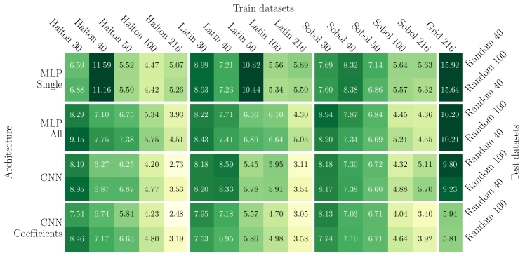
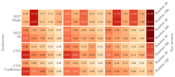
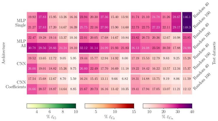
The key insight of the present study is to define a fast model to predict the aerodynamic loads for a pitching airfoil incurring in light and deep dynamic stall. The gradual increase of complexity in the neural network architectures has been driven by the need of a more robust prediction while maintaining the inference time as low as possible. The prediction error of an entire dataset is computed as the average error of the predicted coefficients per each simulation as reported in Equation 3. In detail, $n_{s}$ is the number of simulations in the dataset and ${\varepsilon_{s}}^{2}$ is the squared error of the single snapshot per each coefficient. The error of the single simulation is derived as in Equation 4 in which $n_{t}$ is the number of time steps, namely 3600, $\hat{x}_{s,t}$ is the predicted coefficient at time $t$ in simulation $s$, and $x_{s,t}$ is the reference value. The reason for summing up the squared errors and dividing them by the sum of the reference values is linked to values close to zero. Indeed, when the ground truth value is close to zero, like in the $C_{m}$, a small discrepancy in the predicted value can lead to large relative errors giving a wrong estimation.

$$\bar{\varepsilon} =\sqrt{\frac{\sum_{s=1}^{n_{s}}{\varepsilon_{\text{s}}}^{2}}{n_{s}}}$$ (3)

$${\varepsilon_{\text{s}}}^{2} =\frac{\sum_{t=1}^{n_{t}}\left(\hat{x}_{s,t}-x_{s,t}\right)^{2}}{\sum_{t=1}^{n_{t}}{x_{s,t}}^{2}}$$ (4)

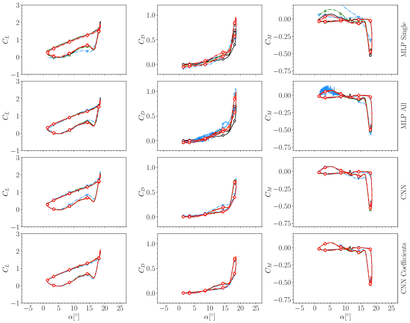
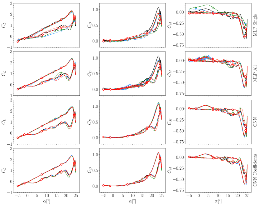
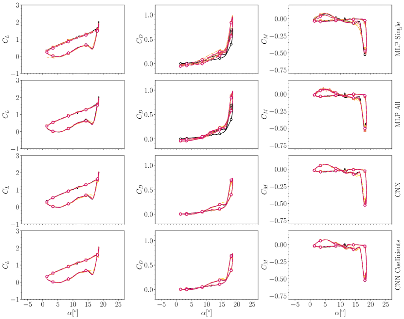
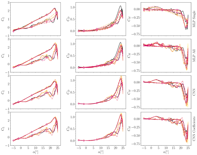
The mean error is able to give the overall performance of each architecture. Since we are also interested in the performance for specific flight settings, two test cases have been selected from the 100-point random dataset to investigate a light and a deep dynamic stall conditions. The light dynamic stall is characterized by an oscillation amplitude of $8.62^{\circ}$, a 18.96 m/s free-stream velocity and a reduced frequency of 0.157. The deep dynamic stall, instead, has an oscillation amplitude of $14.99^{\circ}$, a 15.71 m/s free-stream velocity and a reduced frequency of 0.105. In Figure 8, the mean lift, drag, and momentum coefficient relative errors are compared for all the analyzed architectures with all the train and test datasets. The following two figures, 9 and 10, show the influence of the point distribution of the training datasets maintaining the number of points constant for the aerodynamic loads in the selected test cases. Figures 11 and 12, instead, investigate the effect of the point number for the Halton sequence for the same test cases.

Focusing on the “MLP Single” neural network, the first aspect to notice is the sensitivity to the point distribution. Indeed, when using the uniform grid the $C_{m}$ error is not acceptable and it is several times larger than the other datasets. Another critical point is related to the fact that, for the same low discrepancy sequence, when increasing the number of training points the error is not following any particular trend, making it not usable in real applications. Looking at the predicted coefficients for the chosen test cases we can see that the trends are well captured for lift and drag. The momentum, instead, is in good agreement with the reference data only with the Halton and Latin hypercube datasets, even if for the deep dynamic stall case is completely missing the oscillations in both upstroke and downstroke phases. The architecture suffers particularly in the $C_{m}$ prediction. One of the reasons leading to large mean error is that the predicted curve is not a closed loop suggesting that the underlying physics is not learned.

Since the first architecture was not able to accurately predict the aerodynamic loads, the “MLP All” neural network has been implemented. The idea of considering the entire cycle as output aims at providing more information to the NN in order to learn the relation between subsequent time steps and overcome the previous issues. According to the mean errors reported in Figure 8, the model better catches the physics of the problem. In particular, it is less sensitive to the point distribution used for the training and also the uniform grid one shows errors comparable to low discrepancy ones even if they are higher. Furthermore, enlarging the train datasets results in monotonically decreasing errors as expected. Despite the promising properties shown in the mean error map, when the actual predictions are analyzed, another key issue arises. Especially the drag and momentum curves show spurious non-physical oscillations at low angle of attack making the model not applicable to real world scenarios. Additional layers have been included in the architecture and also a wider number of neurons has been tried but the oscillations are always present. This last aspect encouraged the change of network type and also the output.

The convolutional neural network, coupled with the $C_{p}$ and $C_{f}$ distributions as output, is an effective solution to all the previous problems. Numerical simulations, indeed, are capable of computing a large amount of data and are perfectly suited to be used in conjunctions with data-driven methods like the one presented in this work. However, to build a robust model only the data-driven approach is usually not sufficient, as shown by previous NN examples, and physics information have to be included in the model [65]. The required error convergence property increasing the number of points in each dataset and the low sensitivity to sequence type are satisfied as depicted in the error map. Looking closely in this regard, adding the physics-based loss further improves the performance. Even when the uniform grid distribution is adopted the error is comparable to the other distributions, confirming the necessity of include as many physical relations as possible in the model. The mean error in the “CNN Coefficient” architecture is always lower than the “CNN” one. Furthermore, the error always goes down when using a larger dataset with the more sophisticated loss. On the contrary, the “CNN” has a peak in the mean error for 100-point Latin hypercube and 216-point Sobol’ sequences. The Halton sequence is the one that reaches the lowest global error, but at the same time it is the one that has the largest error when using less points. The Latin and Sobol’ ones, instead, present a more limited error variation while reaching satisfying performances for 100 and 216 points. Overall, the Latin hypercube grants better prediction quality with respect to Sobol. To further remark the effect of physics information in the model, in Figures 9 and 10 it can be noted how the curves for all the three coefficients are closer to the actual solution and the differences of the datasets are less noticeable.

Figure 13: CNN performance comparison for a light dynamic stall example, corresponding to an oscillation amplitude of $8.62^{\circ}$, a 18.96 m/s free-stream velocity and a reduced frequency of 0.157.

Figure 14: CNN performance comparison for a deep dynamic stall example, corresponding to an oscillation amplitude of $14.99^{\circ}$, a 15.71 m/s free-stream velocity and a reduced frequency of 0.105.

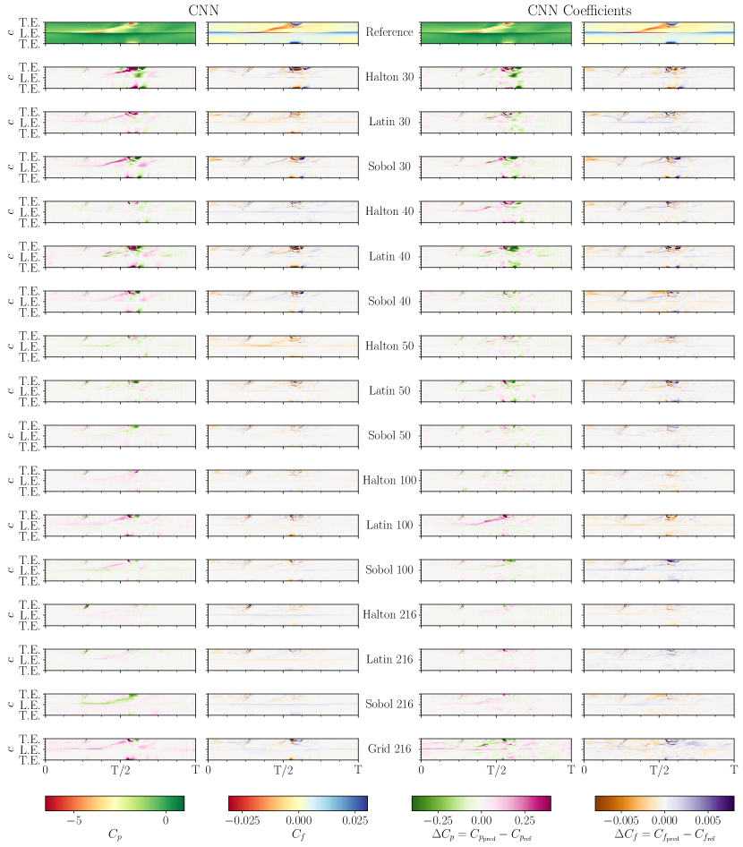
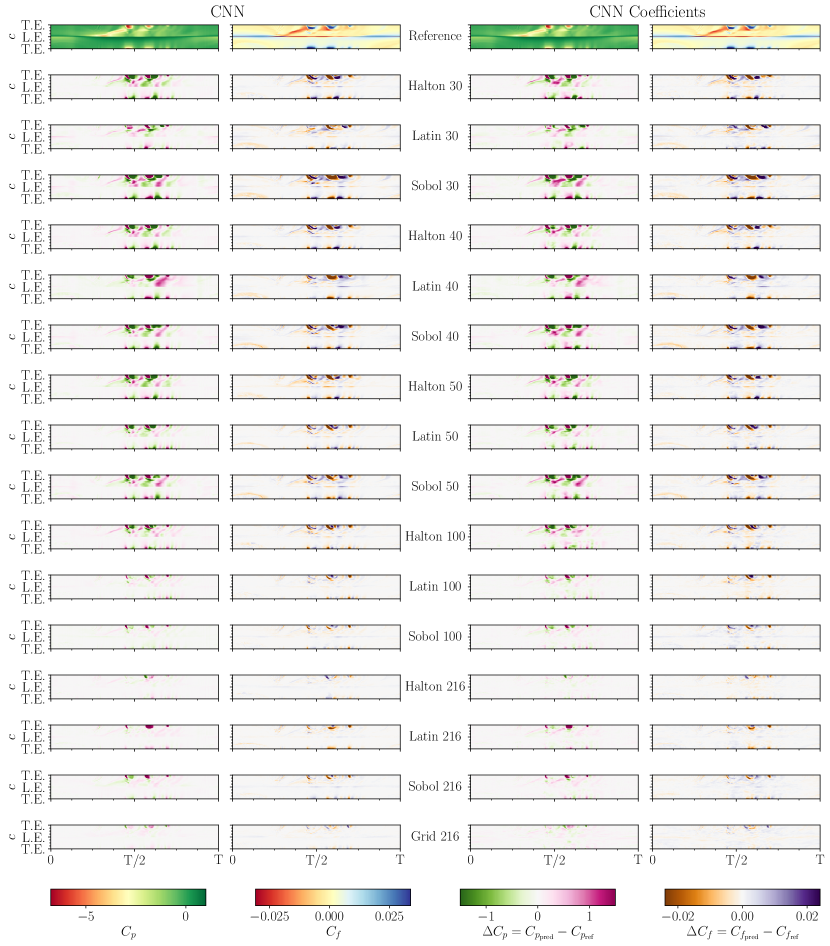
A final comparison is provided for the actual output of CNN based architectures, and it is reported in Figures 13 and 14 in which the reference $C_{p}$ and $C_{f}$ distributions are reported with the absolute error for all the employed train datasets. Looking at the pressure and skin friction over the airfoil, the reasons of the discrepancies are highlighted. A common issue is the ability to capture the instabilities near the trailing edge during the upstroke phase due to the transitioning of the boundary layer from laminar to turbulent. This behavior is due to the up-sampling operations of the flow field that tends to smear out rapid oscillations. The other region where the error is larger coincides with the pressure peaks especially for the secondary vortex that involves highly non-linear phenomena and reaches $C_{p}$ values close to the dynamic stall vortex that detaches first. A peculiarity that seems in contrast to what has been discussed until now is the extremely low error for the uniform grid in the deep dynamic stall case. However, this behavior is due to another effect, that is the distance between the predicted point and the closest training point in the flight envelope. Specifically, for this case, the closest training point is located at $\alpha=15^{\circ}$, $V_{\infty}=16$ m/s, and $k=0.1$ which is particularly near to the deep dynamic stall test conditions.

V Conclusions and final remarks

This work presents a robust framework to fast predict aerodynamic loads for sinusoidal pitching airfoils incurring in light and deep dynamic stall. Deep neural networks are leveraged to build a data-driven model that accurately describes dynamic stall phenomena. Three different architectures have been presented ranging from multilayer perceptrons to convolutional neural networks. A physics-based loss function that incorporates the computation of lift, drag, and momentum coefficients in the network has been implemented, highlighting the advantages of including physical knowledge in the model. Moreover, a periodic condition has been implemented in the convolution layers to ensure the physical meaning of the $C_{p}$ and $C_{f}$ outputs. Indeed, periodicity grants that there are no discontinuities in the distributions over the airfoil and also that the aerodynamic loads are continuous between subsequent cycles. Furthermore, an extensive analysis of the train dataset point distributions has been performed. A uniform grid distribution is compared against low discrepancy sequences: Latin hypercube, Sobol, and Halton for different dataset sizes creating a map of the average error.

The convolutional neural network, coupled with the physics-based loss function, showed unprecedented performance in predicting aerodynamic loads for a broad range of flight conditions in the prescribed flight envelope. In addition, it has been proven that the neural network is slightly influenced by the train point distribution, even if the Latin hypercube is the one that closely predicts the reference loads. Another fundamental feature of the model is the monotonically decreasing error, over the test datasets, when the train datasets have a larger number of points. Despite the limitations of using three parameters to describe the flight envelope and considering incompressible CFD solutions, the properties of the presented framework are still valid for a full compressible setup, and it is a candidate to fill the gap of next-generation reduced order models for dynamic stall phenomena.

References

- Gardner et al. [2023] A. D. Gardner, A. R. Jones, K. Mulleners, J. W. Naughton, and M. J. Smith, Review of rotating wing dynamic stall: Experiments and flow control, Progress in Aerospace Sciences 137, 100887 (2023).
- Corke and Thomas [2015] T. C. Corke and F. O. Thomas, Dynamic stall in pitching airfoils: Aerodynamic damping and compressibility effects, Annual Review of Fluid Mechanics 47, 479 (2015).
- Gardner et al. [2019] A. Gardner, C. Wolf, and M. Raffel, Review of measurement techniques for unsteady helicopter rotor flows, Progress in Aerospace Sciences 111, 100566 (2019).
- Marilyn J. et al. [2020] S. Marilyn J., A. D. Gardner, R. Jain, P. David, and F. Richez, Rotating wing dynamic stall: State of the art and future directions, in 76th Annual Forum & Technology Display Vertical Flight Society (2020).
- Khalifa et al. [2023] N. M. Khalifa, A. Rezaei, and H. E. Taha, On computational simulations of dynamic stall and its three-dimensional nature, Physics of Fluids 35, 105143 (2023).
- Zanotti et al. [2014a] A. Zanotti, R. Nilifard, G. Gibertini, A. Guardone, and G. Quaranta, Assessment of 2D/3D numerical modeling for deep dynamic stall experiments, Journal of Fluids and Structures 51, 97 (2014a).
- De Vanna et al. [2023a] F. De Vanna, G. Baldan, F. Picano, and E. Benini, Effect of convective schemes in wall-resolved and wall-modeled LES of compressible wall turbulence, Computers & Fluids 250, 105710 (2023a).
- De Vanna et al. [2023b] F. De Vanna, G. Baldan, F. Picano, and E. Benini, On the coupling between wall-modeled LES and immersed boundary method towards applicative compressible flow simulations, Computers & Fluids 266, 106058 (2023b).
- Damiola et al. [2023a] L. Damiola, M. F. Siddiqui, M. C. Runacres, and T. De Troyer, Influence of free-stream turbulence intensity on static and dynamic stall of a NACA 0018 aerofoil, Journal of Wind Engineering and Industrial Aerodynamics 232, 105270 (2023a).
- Zanotti and Gibertini [2013] A. Zanotti and G. Gibertini, Experimental investigation of the dynamic stall phenomenon on a NACA 23012 oscillating airfoil, Proceedings of the Institution of Mechanical Engineers, Part G: Journal of Aerospace Engineering 227, 1375 (2013).
- Zanotti et al. [2014b] A. Zanotti, S. Melone, R. Nilifard, and A. D’Andrea, Experimental-numerical investigation of a pitching airfoil in deep dynamic stall, Proceedings of the Institution of Mechanical Engineers, Part G: Journal of Aerospace Engineering 228, 557 (2014b).
- Visbal and Garmann [2018] M. R. Visbal and D. J. Garmann, Analysis of dynamic stall on a pitching airfoil using high-fidelity Large-Eddy Simulations, AIAA Journal 56, 46 (2018).
- Miotto et al. [2022] R. Miotto, W. Wolf, D. Gaitonde, and M. Visbal, Analysis of the onset and evolution of a dynamic stall vortex on a periodic plunging aerofoil, Journal of Fluid Mechanics 938, A24 (2022).
- Hammer et al. [2021] P. R. Hammer, D. J. Garmann, and M. Visbal, Aspect ratio effect on finite wing dynamic stall, in AIAA Scitech 2021 Forum (2021).
- Hammer et al. [2022] P. R. Hammer, D. J. Garmann, and M. R. Visbal, Effect of aspect ratio on finite-wing dynamic stall, AIAA Journal 60, 6581 (2022).
- Hammer et al. [2023] P. R. Hammer, D. J. Garmann, and M. R. Visbal, Effect of aspect ratio on swept-wing dynamic stall, AIAA Journal 61, 4367 (2023).
- Benton and Visbal [2020] S. I. Benton and M. R. Visbal, Effects of compressibility on dynamic-stall onset using large-eddy simulation, AIAA Journal 58, 1194 (2020).
- Beddoes [1976] T. S. Beddoes, A synthesis of unsteady aerodynamic effects including stall hysteresis, Vertica 1, 113 (1976).
- Beddoes [1978] T. S. Beddoes, Onset of leading edge separation effects under dynamic conditions and low mach number, in 34th Annual Forum of the American Helicopter Society (1978).
- Leishman et al. [1986] J. G. Leishman, T. S. Beddoes, and W. H. Ltd, A generalised model for airfoil unsteady aerodynamic behaviour and dynamic stall using the indicial method (1986).
- Leishman [1988] J. G. Leishman, Validation of approximate indicial aerodynamic functions for two-dimensional subsonic flow, Journal of Aircraft 25, 914 (1988).
- Leishman and Beddoes [1989] J. G. Leishman and T. S. Beddoes, A semi-empirical model for dynamic stall, Journal of The American Helicopter Society 34, 3 (1989).
- Leishman [1989] J. Leishman, State-space model for unsteady airfoil behavior and dynamic stall, in 30th Structures, Structural Dynamics and Materials Conference (1989).
- Leishman and Nguyen [1990] J. G. Leishman and K. Q. Nguyen, State-space representation of unsteady airfoil behavior, AIAA Journal 28, 836 (1990).
- Beddoes [1993] T. S. Beddoes, A third generation model for unsteady aerodynamics and dynamic stall, in Technical Report RP-908 (Westland Helicopter Limited, 1993).
- Tran and Falchero [1981] C. T. Tran and D. Falchero, Application of the ONERA dynamic stall model to a helicopter rotor blade in forward flight, in 7th European Rotorcraft Forum (1981).
- Tran and Petot [1981] C. T. Tran and D. Petot, Semi-empirical model for the dynamic stall of airfoils in view of the application to the calculation of the responses of a helicopter blade in forward flight, (1981).
- Truong [1993] V. K. Truong, A 2-D dynamic stall model based on a hopf bifurcation, in 19th European Rotorcraft Forum (1993).
- Truong [1996] V. K. Truong, Prediction of helicopter rotor airloads based on physical modeling of 3-D unsteady aerodynamics, in 22nd European Rotorcraft Forum (1996).
- Lumley [1967] J. Lumley, The structure of inhomogeneous turbulent flows. in atmospheric turbulence and radio wave propagation, The Structure of Inhomogeneous Turbulent Flows , 166 – 178 (1967).
- Rowley et al. [2009] C. W. Rowley, I. Mezic, S. Bagheri, P. Schlatter, and D. S. Henningson, Spectral analysis of nonlinear flows, Journal of Fluid Mechanics 641, 115–127 (2009).
- Schmid [2010] P. J. Schmid, Dynamic mode decomposition of numerical and experimental data, Journal of Fluid Mechanics 656, 5–28 (2010).
- Avanzi et al. [2021] F. Avanzi, F. De Vanna, Y. Ruan, and E. Benini, Design-assisted of pitching aerofoils through enhanced identification of coherent flow structures, Designs 5, 10.3390/designs5010011 (2021).
- Avanzi et al. [2022] F. Avanzi, F. D. Vanna, Y. Ruan, and E. Benini, Enhanced identification of coherent structures in the flow evolution of a pitching wing, in AIAA SCITECH 2022 Forum (2022).
- Chiu et al. [2023] T.-Y. Chiu, C.-C. Tseng, C.-C. Chang, and Y.-J. Chou, Vorticity forces of coherent structures on the naca0012 aerofoil, Journal of Fluid Mechanics 974, A52 (2023).
- Taha et al. [2021] H. E. Taha, L. Pla Olea, N. Khalifa, C. Gonzalez, and A. S. Rezaei, Geometric-control formulation and averaging analysis of the unsteady aerodynamics of a wing with oscillatory controls, Journal of Fluid Mechanics 928, A30 (2021).
- Olea et al. [2022] L. P. Olea, N. M. Khalifa, and H. E. Taha, Geometric control study of the Beddoes-Leishman model in a pitching-plunging airfoil, in AIAA SCITECH 2022 Forum (2022).
- Tatar and Sabour [2020] M. Tatar and M. H. Sabour, Reduced-order modeling of dynamic stall using neuro-fuzzy inference system and orthogonal functions, Physics of Fluids 32, 045101 (2020).
- Glaz et al. [2013] B. Glaz, P. P. Friedmann, L. Liu, J. G. Cajigas, J. Bain, and L. N. Sankar, Reduced-order dynamic stall modeling with swept flow effects using a surrogate-based recurrence framework, AIAA Journal 51, 910 (2013).
- Vinuesa et al. [2023] R. Vinuesa, S. L. Brunton, and B. J. McKeon, The transformative potential of machine learning for experiments in fluid mechanics, Nature Reviews Physics 5, 536 (2023).
- Chen and Thuerey [2023] L.-W. Chen and N. Thuerey, Towards high-accuracy deep learning inference of compressible flows over aerofoils, Computers & Fluids 250, 105707 (2023).
- Eivazi et al. [2022a] H. Eivazi, M. Tahani, P. Schlatter, and R. Vinuesa, Physics-informed neural networks for solving Reynolds-averaged Navier–Stokes equations, Physics of Fluids 34, 075117 (2022a).
- Bragone et al. [2022a] F. Bragone, K. Oueslati, T. Laneryd, M. Luvisotto, and K. Morozovska, Physics-informed neural networks for modeling cellulose degradation in power transformers, in 2022 21st IEEE International Conference on Machine Learning and Applications (ICMLA) (2022) pp. 1365–1372.
- Bragone et al. [2022b] F. Bragone, K. Morozovska, P. Hilber, T. Laneryd, and M. Luvisotto, Physics-informed neural networks for modelling power transformer’s dynamic thermal behaviour, Electric Power Systems Research 211, 108447 (2022b).
- Baldan et al. [2021] M. Baldan, G. Baldan, and B. Nacke, Solving 1D non-linear magneto quasi-static Maxwell’s equations using neural networks, IET Science, Measurement & Technology 15, 204 (2021).
- Baldan et al. [2023] M. Baldan, P. Di Barba, and D. A. Lowther, Physics-Informed neural networks for inverse electromagnetic problems, IEEE Transactions on Magnetics 59, 1 (2023).
- Guastoni et al. [2021] L. Guastoni, A. Güemes, A. Ianiro, S. Discetti, P. Schlatter, H. Azizpour, and R. Vinuesa, Convolutional-network models to predict wall-bounded turbulence from wall quantities, Journal of Fluid Mechanics 928, A27 (2021).
- Eivazi et al. [2022b] H. Eivazi, S. Le Clainche, S. Hoyas, and R. Vinuesa, Towards extraction of orthogonal and parsimonious non-linear modes from turbulent flows, Expert Systems with Applications 202, 117038 (2022b).
- Lennie et al. [2020] M. Lennie, J. Steenbuck, B. R. Noack, and C. O. Paschereit, Cartographing dynamic stall with machine learning, Wind Energy Science 5, 819 (2020).
- Kasmaiee et al. [2023] S. Kasmaiee, M. Tadjfar, and S. Kasmaiee, Machine learning-based optimization of a pitching airfoil performance in dynamic stall conditions using a suction controller, Physics of Fluids 35, 095121 (2023).
- Damiola et al. [2023b] L. Damiola, J. Decuyper, M. Runacres, and T. D. Troyer, Modeling airfoil dynamic stall using State-Space Neural Networks, in AIAA SCITECH 2023 Forum (2023).
- Eivazi et al. [2020] H. Eivazi, H. Veisi, M. H. Naderi, and V. Esfahanian, Deep neural networks for nonlinear model order reduction of unsteady flows, Physics of Fluids 32, 105104 (2020).
- Solera-Rico et al. [2023] A. Solera-Rico, C. S. Vila, M. A. Gómez, Y. Wang, A. Almashjary, S. T. M. Dawson, and R. Vinuesa, -variational autoencoders and transformers for reduced-order modelling of fluid flows (2023), arXiv:2304.03571 [physics.flu-dyn] .
- Wang et al. [2024] Y. Wang, A. Solera-Rico, C. Sanmiguel Vila, and R. Vinuesa, Towards optimal -variational autoencoders combined with transformers for reduced-order modelling of turbulent flows, International Journal of Heat and Fluid Flow 105, 109254 (2024).
- Lee and Gerontakos [2004] T. Lee and P. Gerontakos, Investigation of flow over an oscillating airfoil, Journal of Fluid Mechanics 512, 313–341 (2004).
- Baldan and Guardone [2023] G. Baldan and A. Guardone, Pattern recognition of the flow around a pitching NACA 0012 airfoil in dynamic stall conditions, in Aeronautics and Astronautics (2023).
- Menter et al. [2004] F. R. Menter, R. B. Langtry, S. R. Likki, Y. B. Suzen, P. G. Huang, and S. Völker, A correlation-based transition model using local variables – Part I: Model formulation, Journal of Turbomachinery , 413 (2004).
- Kocis and Whiten [1997] L. Kocis and W. J. Whiten, Computational investigations of low-discrepancy sequences, ACM Trans. Math. Softw. 23, 266–294 (1997).
- Virtanen et al. [2020] P. Virtanen, R. Gommers, T. E. Oliphant, M. Haberland, T. Reddy, D. Cournapeau, E. Burovski, P. Peterson, W. Weckesser, J. Bright, S. J. van der Walt, M. Brett, J. Wilson, K. J. Millman, N. Mayorov, A. R. J. Nelson, E. Jones, R. Kern, E. Larson, C. J. Carey, İ. Polat, Y. Feng, E. W. Moore, J. VanderPlas, D. Laxalde, J. Perktold, R. Cimrman, I. Henriksen, E. A. Quintero, C. R. Harris, A. M. Archibald, A. H. Ribeiro, F. Pedregosa, P. van Mulbregt, and SciPy 1.0 Contributors, SciPy 1.0: Fundamental Algorithms for Scientific Computing in Python, Nature Methods 17, 261 (2020).
- Cybenko [1989] G. Cybenko, Approximation by superpositions of a sigmoidal function, Mathematics of Control, Signals and Systems 2, 303 (1989).
- Albawi et al. [2017] S. Albawi, T. A. Mohammed, and S. Al-Zawi, Understanding of a convolutional neural network, in 2017 International Conference on Engineering and Technology (ICET) (2017) pp. 1–6.
- Xu et al. [2015] B. Xu, N. Wang, T. Chen, and M. Li, Empirical evaluation of rectified activations in convolutional network (2015), arXiv:1505.00853 [cs.LG] .
- Kingma and Ba [2014] D. P. Kingma and J. Ba, Adam: A method for stochastic optimization, CoRR abs/1412.6980, 10.48550/arXiv.1412.6980 (2014).
- Choquette et al. [2021] J. Choquette, W. Gandhi, O. Giroux, N. Stam, and R. Krashinsky, Nvidia a100 tensor core gpu: Performance and innovation, IEEE Micro 41, 29 (2021).
- Dias Ribeiro et al. [2023] M. Dias Ribeiro, M. Stradtner, and P. Bekemeyer, Unsteady reduced order model with neural networks and flight-physics-based regularization for aerodynamic applications, Computers & Fluids 264, 105949 (2023).