3D Reconstruction and New View Synthesis of Indoor Environments
based on a Dual Neural Radiance Field
Abstract
Simultaneously achieving 3D reconstruction and new view synthesis for indoor environments has widespread applications but is technically very challenging. State-of-the-art methods based on implicit neural functions can achieve excellent 3D reconstruction results, but their performances on new view synthesis can be unsatisfactory. The exciting development of neural radiance field (NeRF) has revolutionized new view synthesis, however, NeRF-based models can fail to reconstruct clean geometric surfaces. We have developed a dual neural radiance field (Du-NeRF) to simultaneously achieve high-quality geometry reconstruction and view rendering. Du-NeRF contains two geometric fields, one derived from the SDF field to facilitate geometric reconstruction and the other derived from the density field to boost new view synthesis. One of the innovative features of Du-NeRF is that it decouples a view-independent component from the density field and uses it as a label to supervise the learning process of the SDF field. This reduces shape-radiance ambiguity and enables geometry and color to benefit from each other during the learning process. Extensive experiments demonstrate that Du-NeRF can significantly improve the performance of novel view synthesis and 3D reconstruction for indoor environments and it is particularly effective in constructing areas containing fine geometries that do not obey multi-view color consistency.
1 Introduction
3D reconstruction and novel view synthesis for indoor environments are of great interest in the computer vision and graphics communities [16, 10, 52, 13, 1, 26, 27, 18, 19, 56]. They provide fundamental support for applications such as robot perception and navigation, virtual reality, and indoor design. Classical indoor 3D reconstruction methods perform registration and fusion to obtain dense geometry using depth images in an explicit manner where the depth images are obtained either with range sensors like Kinect or inferred from RGB images [9, 15, 28, 7, 17, 37, 48, 12]. However, due to noise and holes in the depth images, complete and accurate indoor geometry is difficult to generate. Additionally, such an explicit representation can often fail to preserve sufficient details due to storage limitations thus making it very difficult to synthesize realistic novel views.
In recent years, coordinate neural networks have been extensively used to describe 3D geometry and appearance due to their powerful implicit and continuous representation capacities [26, 25, 31, 45, 49, 32, 43]. These models take the 3D coordinates as input and output the signed distance value [31, 45, 49], density [26, 27], or occupancy of the scene [25, 32, 43]. Although methods such as Neus [45] and VolSDF [49] can achieve accurate 3D reconstruction of objects, they do not perform well in indoor scenes containing textureless regions or when the observations are sparse. In such cases, depth images are often introduced to provide additional supervision for network training to improve performances [52, 1, 44]. Furthermore, these methods focus on 3D reconstruction and their performances on novel view synthesis can be unsatisfactory.
Neural Radiance Field (NeRF) [26] and a series of its extensions [23, 50, 11, 6, 40, 27, 55, 3, 53, 18, 20, 54, 4, 8, 46] have achieved exciting results in novel view synthesis. It implicitly represents the density field and color field and performs novel view synthesis via volume rendering. However, these methods can fail to reconstruct clean indoor surface as the density used in NeRF samples the whole space rather than in the vicinity of the surfaces.
In this paper, we propose a dual neural radiance field (Du-NeRF) to simultaneously achieve high-quality geometry reconstruction and view rendering. Specifically, our framework contains two geometric fields, one is derived from the SDF field with clear boundary definitions, and the other is a density field that is more conducive to rendering. They share the same underlying input features, which are interpolated from multi-resolution feature grids and then decoded by different decoders. Finally, we enable the two branches to each play their respective strength, while the former is used to extract geometric features, the latter is used to support the task of new view synthesis. In addition, we decouple a view-independent component from the density field and use it as a label to supervise the learning process of SDF during the network optimization process. In our method, the two geometric fields share the underlying input geometric features to facilitate the optimization of the underlying geometric feature grid. Moreover, we use a view-invariant component decoupled from the density branch to replace the view-varying ground truth (GT) images to guide the geometric learning process to reduce shape-radiance ambiguity and allow geometry and color to benefit from each other during the learning process. Experimental results show that this design can effectively construct fine geometries to achieve smooth scene reconstruction, especially in those areas that do not obey multi-view color consistency. Our contributions are as follows:
-
•
We have developed a novel neural radiance field termed Dual Neural Radiance Field (Du-NeRF) for simultaneously improving 3D reconstruction and new view synthesis of indoor environments.
-
•
We introduce a new self-supervised method to derive a view-independent color component that effectively contributes to filling missing parts in 3D reconstruction.
-
•
Extensive experiments demonstrate that our method can significantly improve the performance of novel view synthesis and 3D reconstruction for indoor environments.
2 Related Work
Neural radiance-based novel view synthesis. The introduction of the neural radiance field (NeRF) marks remarkable progress in novel view generation [26]. NeRF models a full-space implicit differentiable and continuous radiance field with neural networks and uses volume rendering to obtain color information. Many variants have been proposed to improve training, inferencing and rendering performances [23, 6, 40, 27, 3, 20, 54, 4, 8, 46]. In particular, DirectVoxelGO [40] and InstantNGP [27] combine explicit and implicit representations and use hybrid grid representations and shallow neural networks for density and color estimation respectively to achieve faster rendering speed and higher rendering quality. Liu et al. [23] introduce a progressive voxel pruning and growing strategy to sample the effective region near the scene surface. Chen et al. [6] use a combination of 2D planes and 1D lines to approximate the grid to achieve faster reconstruction, improved rendering quality, and smaller model sizes. To address the ambiguity arising from pixels represented by a single ray, Barron et al. [3] introduce the concept of cones instead of points, to increase the receptive field of a single ray. This approach, known as Mip-nerf, effectively tackles issues of jaggies and aliasing and enhances rendering quality. To reduce the blurring effect, Lee et al. design a rigid blurry kernel module which takes into account both motion blur and defocus blur during the real acquisition process. Kun et al. further improve the rendering performance by learning a degradation-driven inter-viewpoint mixer [54]. Additionally, some works attempt to improve the rendering performance by jointly optimizing the poses of the training images [4, 8, 46]. In contrast, our method adopts geometry-guided sampling, which benefits from the reconstruction result and allows for more accurate sampling of points near the surface, thus improving the performance of view synthesis.
Neural implicit 3D reconstruction. Neural implicit functions take a 3D location as input and output occupancy, density, and color [25, 32, 30, 26, 29]. Scene Representation Networks employ MLPs to map 3D coordinates to latent features that encode geometry and color information [38]. Yariv et al. [49] and Wang et al. [45] propose two approaches to converting SDF values into density and performing volume rendering to supervise object reconstruction in the Nerf-based framework. Neuralangelo [22] introduces numerical gradients and utilizes multiresolution hash grids to reconstruct detailed scenes. However, while these methods perform well on scenes with rich texture, they struggle with indoor scenes with textureless walls and ceilings. To address these issues, Yu et al. [52] employ predicted depth and normal maps from a pre-trained network to enhance the reconstruction of indoor scenes. Azinović et al. [1] combine a TSDF representation with the NeRF framework and use a depth representation from an off-the-shelf RGBD sensor to improve the accuracy of indoor geometry reconstruction. Subsequent studies [44, 47, 21] have further optimized the Neural-RGBD strategy to speed up training. [44] utilizes voxel representations instead of 3D coordinates to achieve faster query, while [47] trains a dynamically adaptive grid that allocates more voxel resources to more complex objects. [21] pre-trains a feature grid to accelerate the training process. We propose to decouple the view-independent colour component for guiding the 3D reconstruction, which effectively fills in the missing parts of depth-based reconstruction.
3 Method
3.1 Preliminaries
Neural radiance field. Given a collection of posed images, neural radiance field can estimate the color and depth of each pixel by computing the weighted sum of sampling points based on their color and distance from the center of the camera [24]:
| (1) |
where the color and distance from sampling points to the camera center, are denoted by and respectively, are the contribution weights of each sampling point to the color and depth and is calculated as , where and are the density and opacity of sampling point , respectively. The opacity is then computed using Eq. 2.
| (2) |
the color and density of a given sampling point are predicted by the Multi-layer Perceptron (MLP). The process is illustrated in Eq. 3.
| (3) |
where and represent the location and ray direction, respectively. is the feature vector related to the location. and are implicit functions modelled by MLPs.
SDF-based neural implicit reconstruction. The signed distance function (SDF) refers to the nearest distance between a point and surfaces and is often used to implicitly represent geometry. One notable application of SDF is neural implicit reconstruction under the volume rendering framework, achieved by a method called Neus [45].
The key to the success of this method is an unbiased transformation between the SDF values and the density, as demonstrated in Eq. 4. This transformation enables the creation of high-quality surface geometry with great accuracy and cleanliness.
| (4) |
where represents the SDF value of a given sample point, and , while the smoothness of the surface is conditioned on a learnable parameter .
Multi-resolution feature grid. To improve the efficiency of training, a grid representation is used [40, 50, 6]. However, using only single-resolution grid limits the optimization of density and color to local information, resulting in disruptions to the smoothness and continuity of the scene texture [52, 44]. A multi-resolution grid expands the local optimization to nearby continuous fields by varying the receptive field and gradient backpropagation of sample points, enabling higher rendering quality and smoother geometry. The embedding feature is obtained by concatenating the features of each level, as shown in Eq. 5.
| (5) |
where indicates concatenation, and is trilinear interpolation in the -th grid. The final feature vector of the input network is denoted as .
To achieve a higher resolution, hash-based feature grid is employed in [27]. It represents resolutions as:
| (6) |
where , are the coarsest and finest resolution, respectively. represents th level resolution and is the total levels. Similarly, we extract the interpolated features at each level and concatenate them together as in Eq. 5.
3.2 Dual Neural Radiance Field
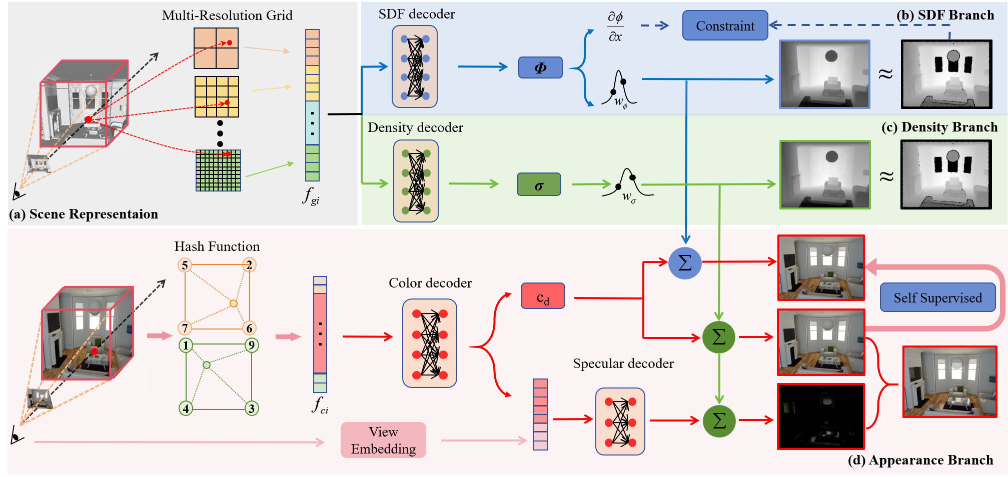
Scene representation. To achieve high-fidelity indoor scene reconstruction and rendering simultaneously, we introduce the dual neural radiance field. The key idea that enables the dual neural radiance field to achieve high-fidelity reconstruction and rendering is to separately represent the geometry field and the color field. Taking into account the fact that the reconstruction task and the rendering task have different complexities, the geometry field and the color field are represented by multi-resolution grids with different levels to speed up training and inference.
As shown in Fig. 1, we use a four-level grid to represent the scene geometry where the grid sizes at each level are respectively 3cm, 6cm, 24cm, and 96cm. At each level, the dimension of the geometry feature is set to 4, and the dimension of the geometry feature is therefore 16. For the color field, the hash-based multi-resolution grid is utilized. The coarsest resolution of the hash-based multi-resolution grid is set to 16. The level of grid resolution is , and the feature vector at each level is -dimensional, we therefore obtain a hash color feature vector with a total of 32 dimensions. The geometry feature and color feature are obtained using tri-linear interpolation.
Dual neural radiance networks. The key idea is to use two different geometric decoders to extract SDF and density, which are respectively used for 3D reconstruction and image rendering. The SDF and density are estimated implicitly from the same interpolated features :
| (7) |
where both of the and are MLPs, and used to decode into SDF and density , respectively. and are both converted to occupancy through Eq. 4 and Eq. 2, respectively. The resulting occupancy of the two is calculated via Eq. 1 to obtain the pixel depth and color. The whole process is supervised with the image reconstruction loss and depth loss.
Sampling points near around object surface have a higher contribution to the rendered color of the ray [26, 45]. To obtain higher rendering quality, we employ the hierarchical sampling strategy as in [26, 45], which contains coarse sampling and fine sampling near the surface. Specifically, we first uniformly sample 96 points along the ray in the coarse stage and then iteratively add 12 sampling points three times according to the cumulative distribution function(CDF) of previous coarse points weights in the fine stage as in [44]. Finally, we got 132 sampling points for depth and color rendering. Note that we use the weight distribution calculated from the SDF branch for sampling as it provides more accurate surface information. For the volume rendering process, the two branches share the sampling points.
Self-supervised color decomposition. We disentangle the color into view-independent color and view-dependent color. We use the decoupled view-independent color to guide geometry learning in a multi-view consistent self-supervised manner by constraining the weight values. This separation allows the color branch to leverage complete color information for rendering, while the geometry branch benefits from view-consistent supervision. Previous work has shown that decoupling colors helps mitigate shape-radiance ambiguity [55, 42]. [42] accomplished the color decomposition supervised by the complete color. In contrast, we not only exploit the complete color to supervise the color decomposition but the view-independent color consistency obtained from the SDF branch and density branch in a self-supervised manner. This design effectively extracts view-independent color to support accurate geometry reconstruction but also boosts the image rendering without any additional specular regularity term as in [33, 42].
To achieve it, as shown in Fig. 1, we utilize two color decoders consisting of MLPs to implicitly estimate the view-independent color and view-dependent color. The view-independent decoder takes the interpolated color feature as input and outputs the view-independent color and an intermediate feature . The specular (view-dependent) decoder takes the intermediate feature and encodes the view vector as input to obtain the specular color . The overall color at a sampling point is calculated by adding the two color components . The final color is generated by summing the weighted color of each sampling point with Eq. 1. In our framework, we integrate with the full color as in NeRF, however, we only weight the view-independent color with to obtain the view-independent color of the corresponding ray. The calculation of color in Eq. 1 becomes:
| (8) |
where is the view-independent color computed by . We can obtain the view-independent color computed by and , which will be used as the ground truth to constrain the learning process of :
| (9) |
3.3 Network training
To optimize the dual neural radiance field, we randomly sample rays during training. Our loss is divided into two components including a loss, and a loss in Eq. 10.
| (10) |
The contains the three components as shown in Eq. 11: view-independent color loss, depth loss and SDF regularization loss, as the following:
| (11) |
The view-independent loss is calculated as the distance between and as shown in Eq. 9, and the depth loss is the loss:
| (12) |
In order to improve the robustness of the learning process of the SDF , we imposed a series of SDF losses to regularize the value as [44]:
| (13) |
The regularization term encourages valid SDF predictions in the unsupervised regions, while is an explicit smoothness term to realize smooth surfaces.
| (14) |
| (15) |
and are used to constrain the truncation distance .
| (16) |
| (17) |
A detailed explanation of these regularity constraints can be found in [44].
The loss contains two parts as shown in Eq. 18:
| (18) |
where is the final rendering color and is the depth calculated from the color branch. is used to align two geometric fields. We experimentally found that is important for decoupling consistent view-independent color. For each of the geometry coefficients, we follow the practice of [44] and set them as follows: , , , , , . For color coefficients we experimentally set them as and .
4 Experiment
4.1 Setup
Implementation details. The SDF decoder , density decoder , color decoder and specular decoder all use two-layers MLPs with the hidden dimension of 32. We sample rays for each iteration, each ray contains coarse samples and fine samples. Our method is implemented in Pytorch and trained with the ADAM optimizer with a learning rate of , and for MLP decoders, multi-resolution grids features, respectively. We run 20K iterations in all scenes with the learning rate decay at iteration 10000 and 15000, and the decay rate is .
Baselines. To validate the effectiveness of the proposed method, we compare it with approaches to indoor 3D reconstruction and view rendering, respectively. For indoor 3D reconstruction, we compare with registration-based method including BundleFusion [10], Colmap [34, 36, 35], Convolutional Occupancy Networks [32], SIREN [39], and recent volumetric rendering-based geometry reconstruction methods such as Neus [45], VolSDF [49], Neural RGBD [1], and Go-Surf [44]. We run marching cubes at the resolution of 1cm to extract meshes. We cull the points and faces in the areas that are not observed in any camera views as in [1, 44]. Besides, the same pose refinement is applied in the same way as in [1, 44].
For image rendering, we compare some representative approaches based on the neural radiance field, including DVGO [40] and InstantNGP [27]. We extract their mesh structures by marching cubes, and compare their geometric metrics and rendering quality. We implement these methods based on SDFstudio [51] and NeRFstudio [41].
NeuralRGBD
Go-Surf
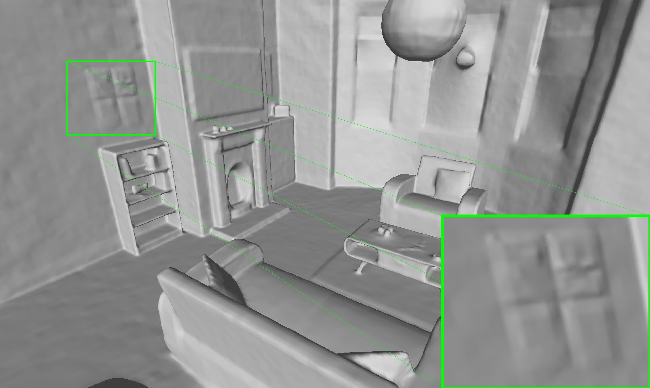
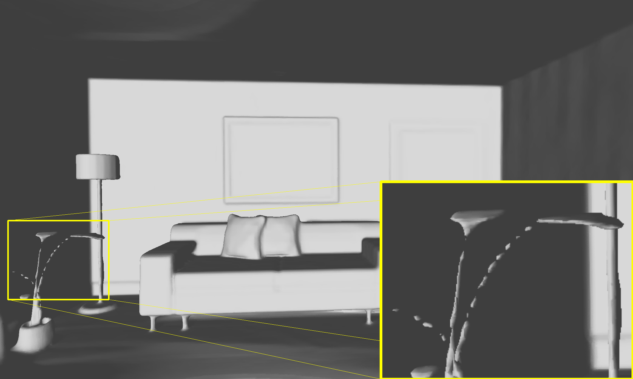
Ours
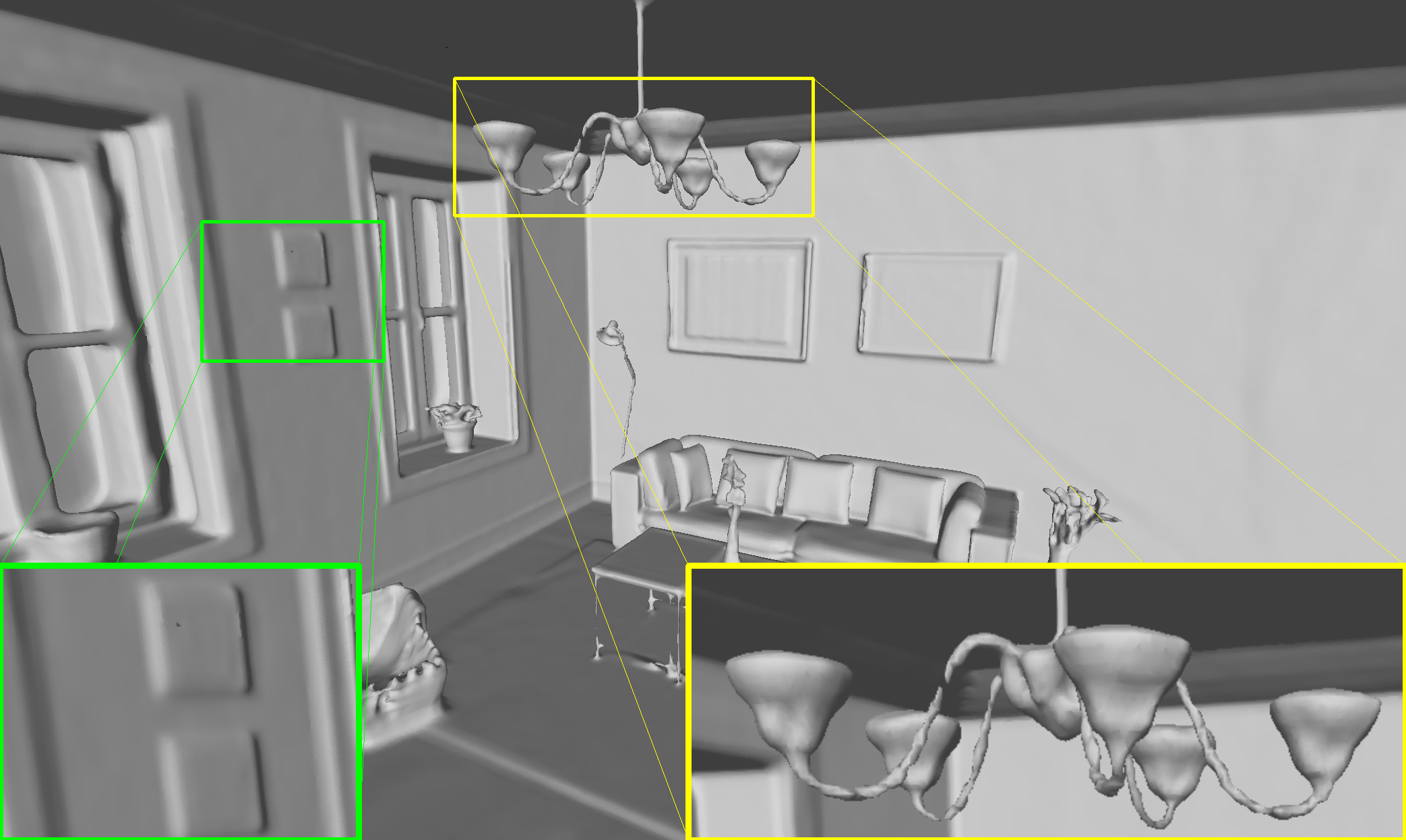
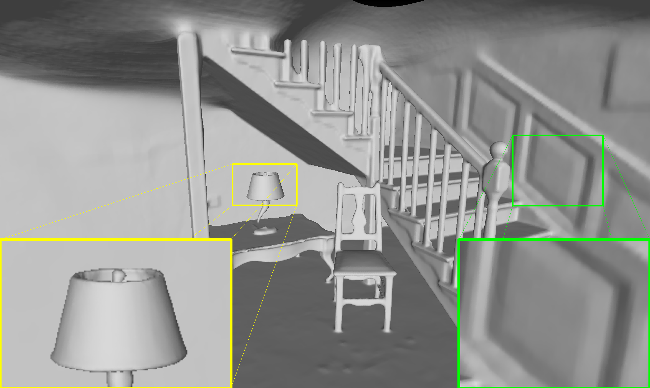
GT
4.2 Comparison
Evaluation on NeuralRGBD Dataset. We evaluated our method on 10 synthesis data used in NeuralRGBD and Go-Surf. The NeuralRGBD dataset consists of 10 synthetic scenes. It provides images, corresponding poses from the Bundlefusion algorithm, and noised depths. The noised depth is used to simulate the collection of real depth sensor Kinect. To compare the image synthesis performance, we choose about of the images as the validation set for image rendering comparison. Specifically, we chose one image from every 10 images of the image sequence as the validation dataset. The first and last images were discarded to avoid the interference of marginal areas that can not observed by the training dataset.
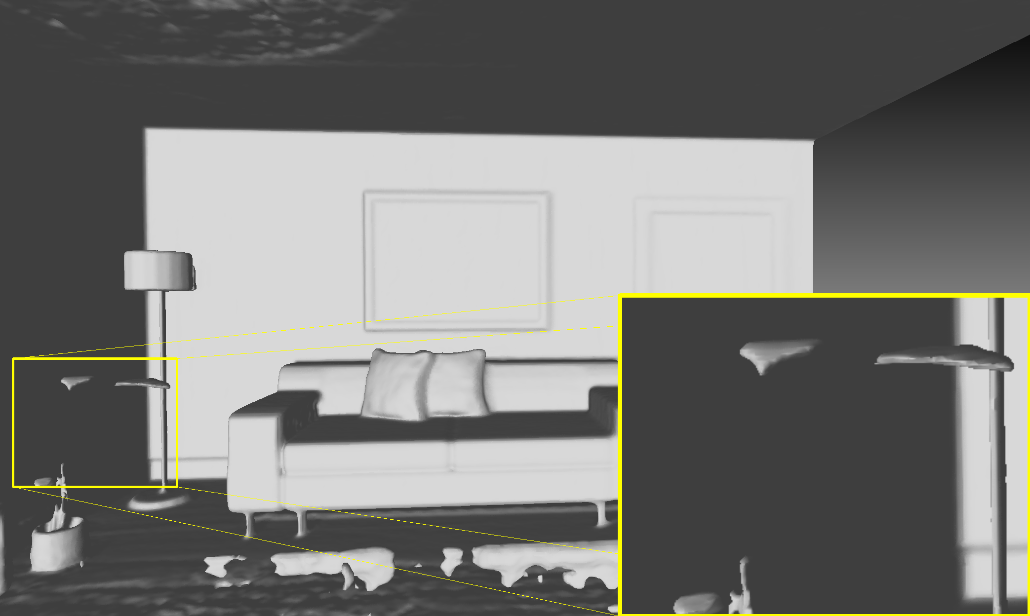
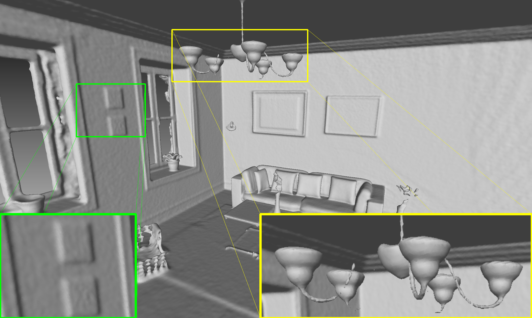
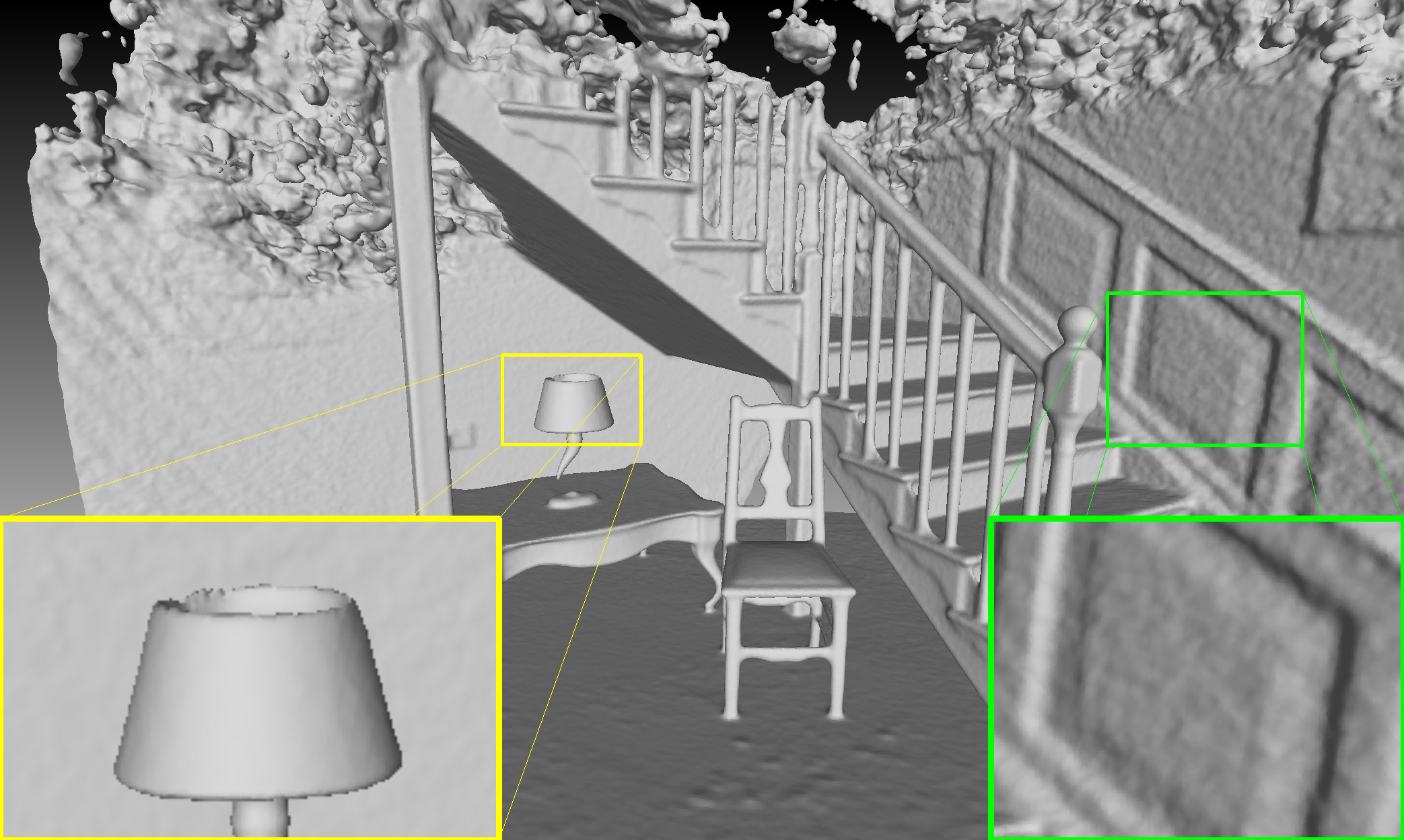
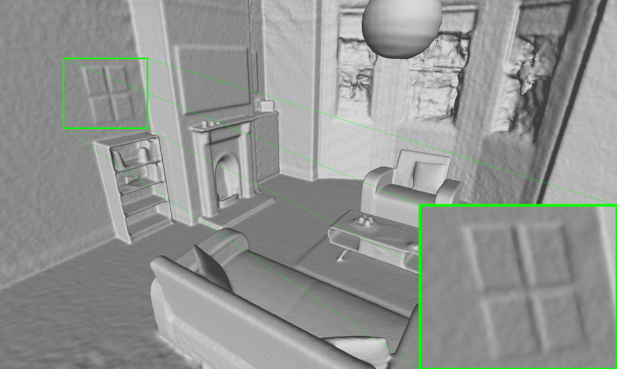
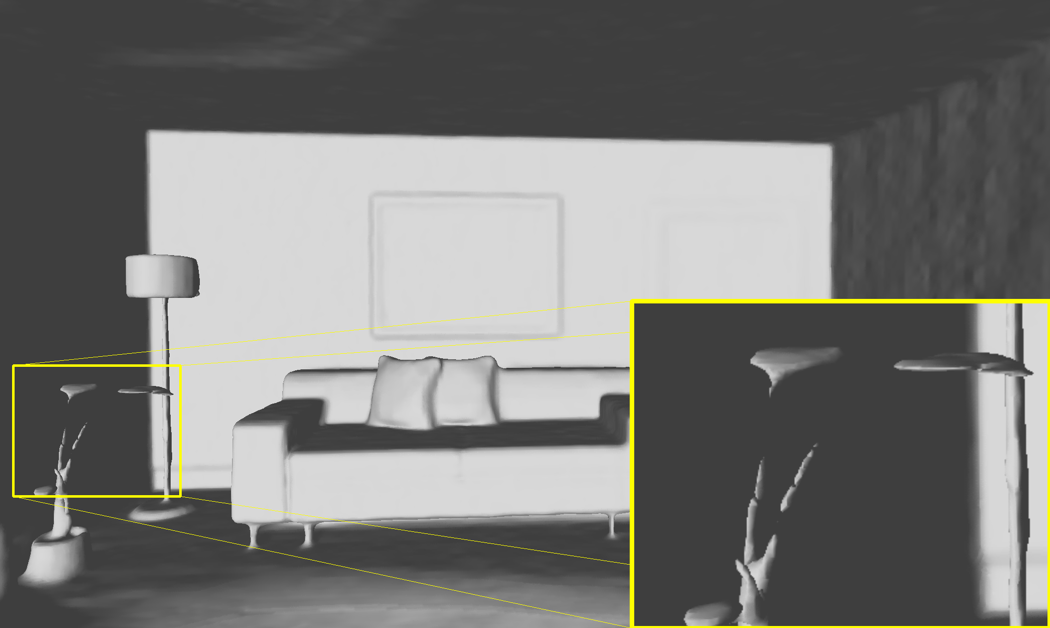
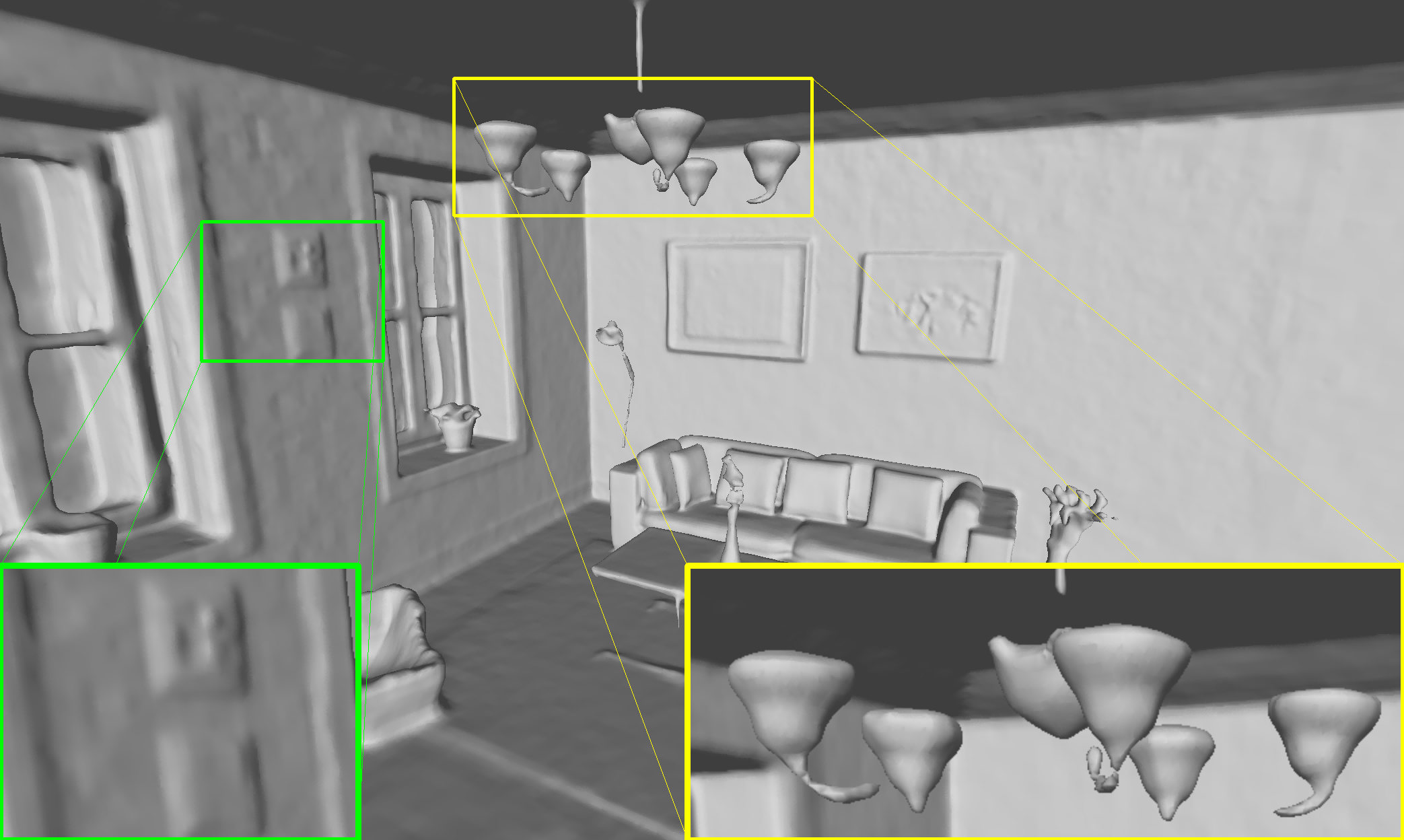
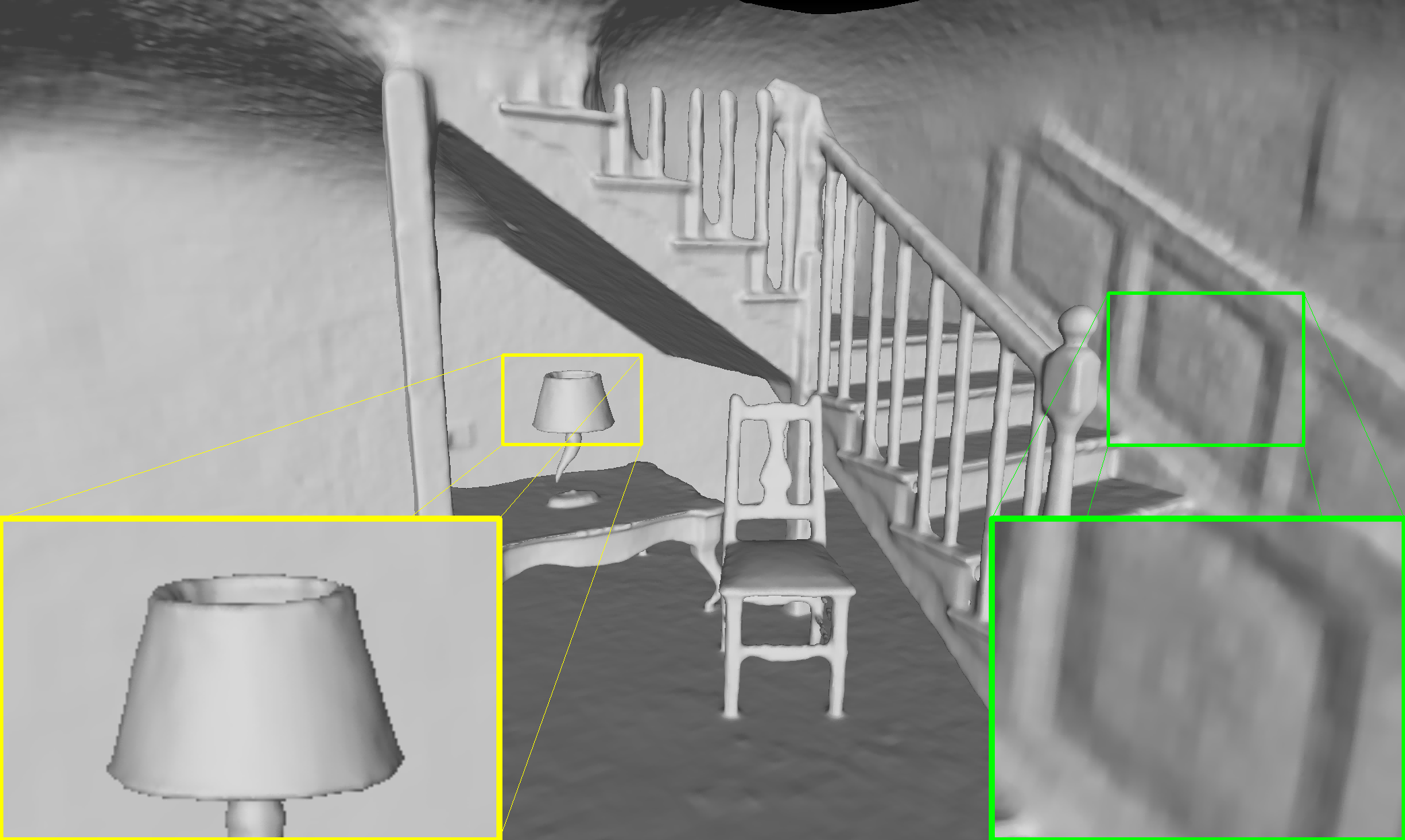
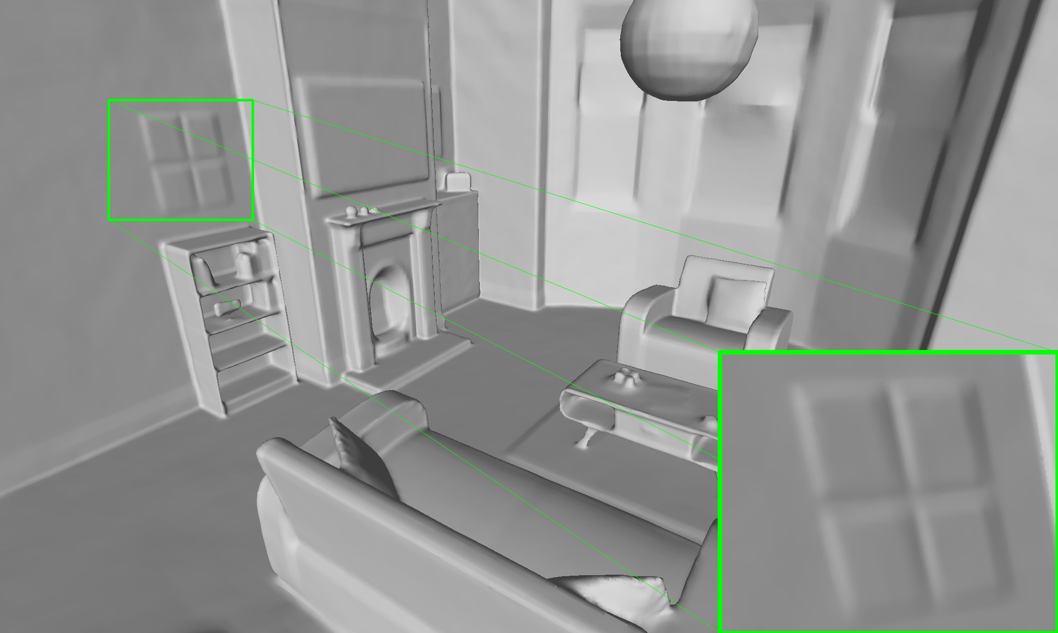
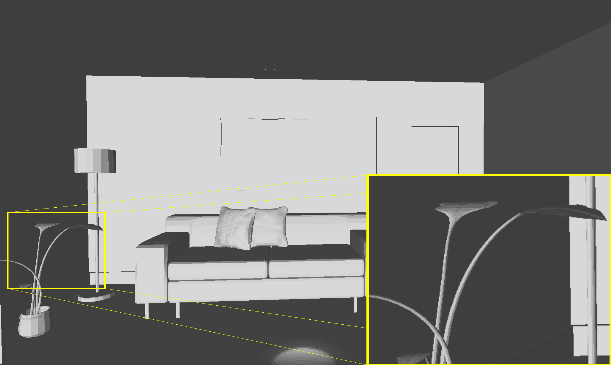
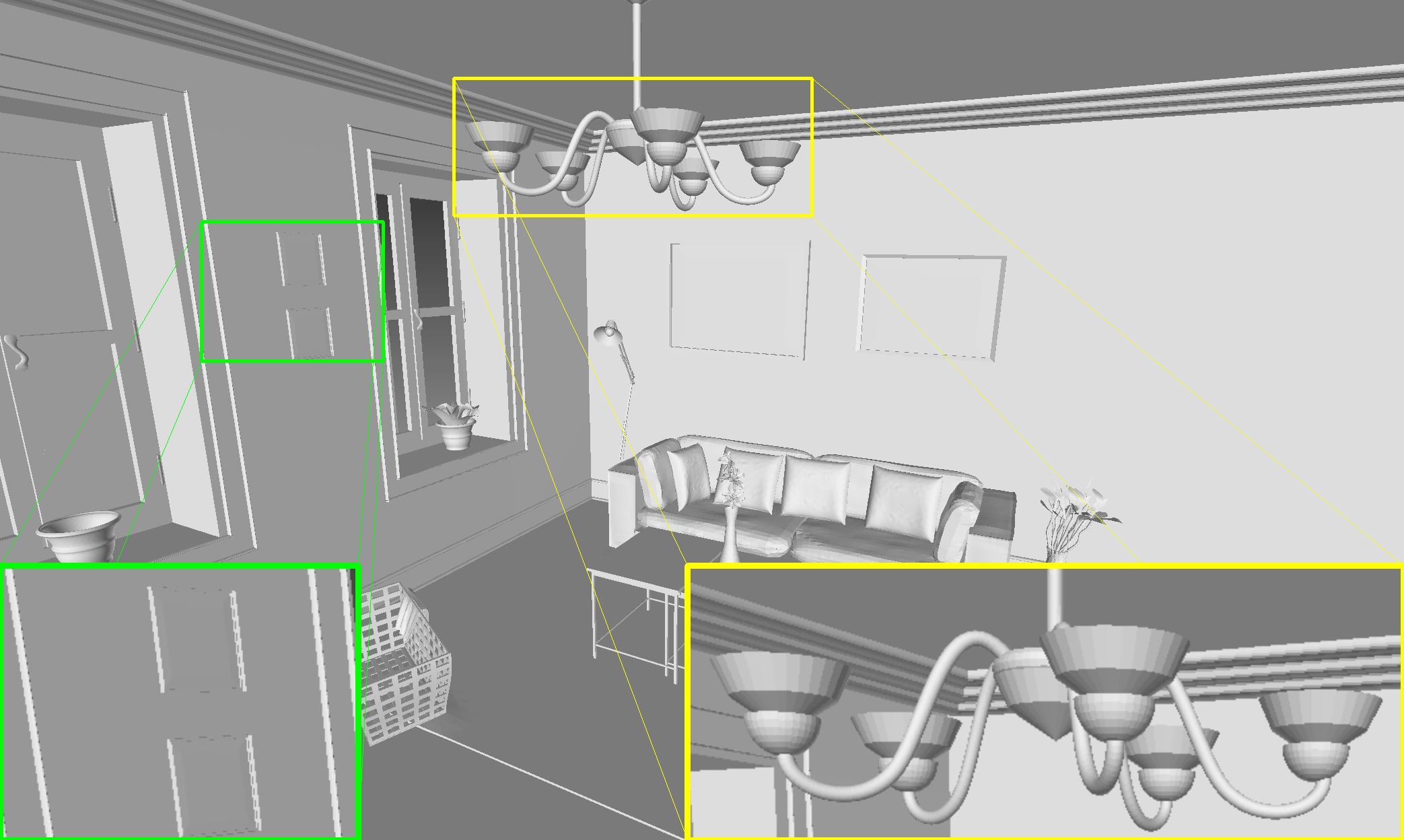
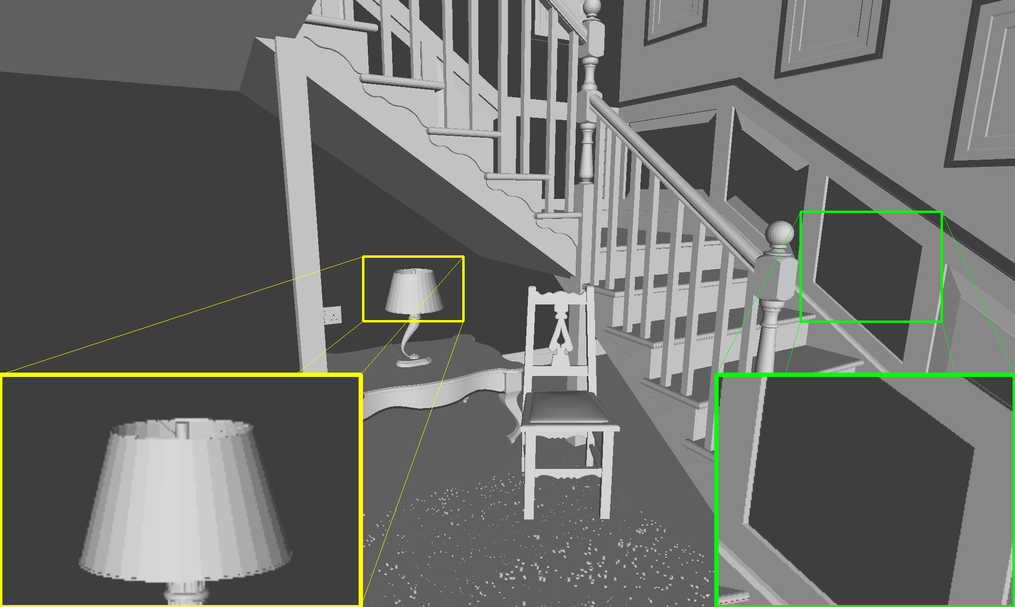
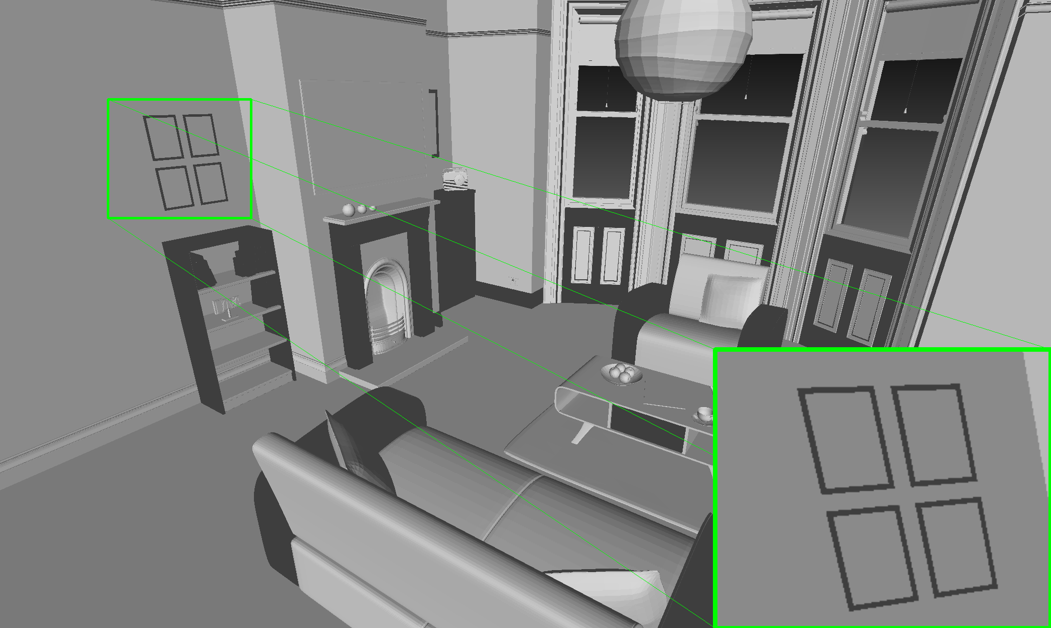
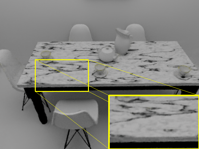
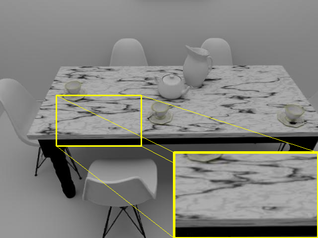
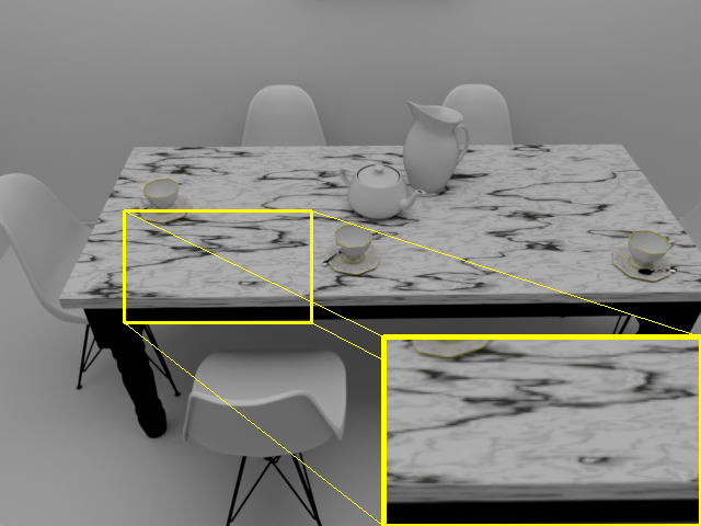
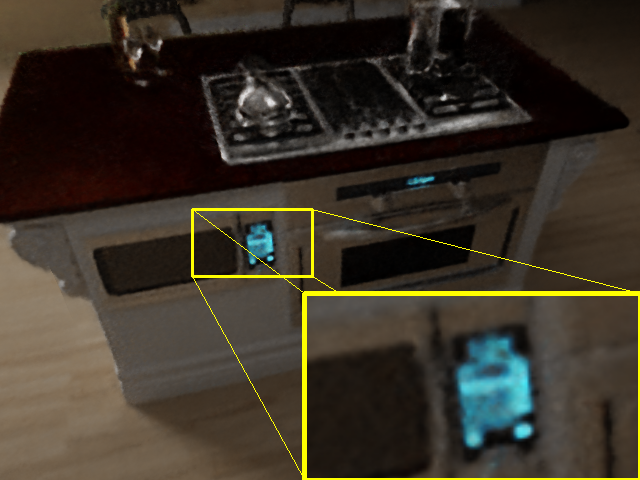
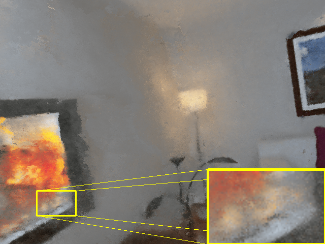
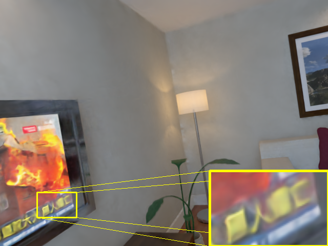
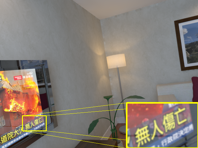
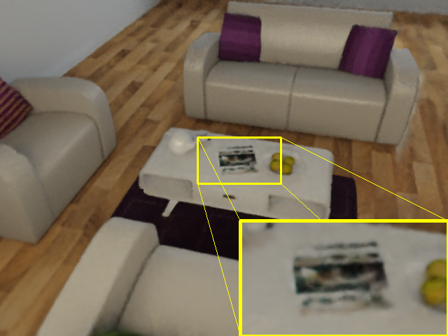
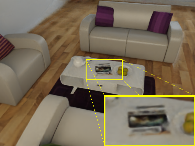
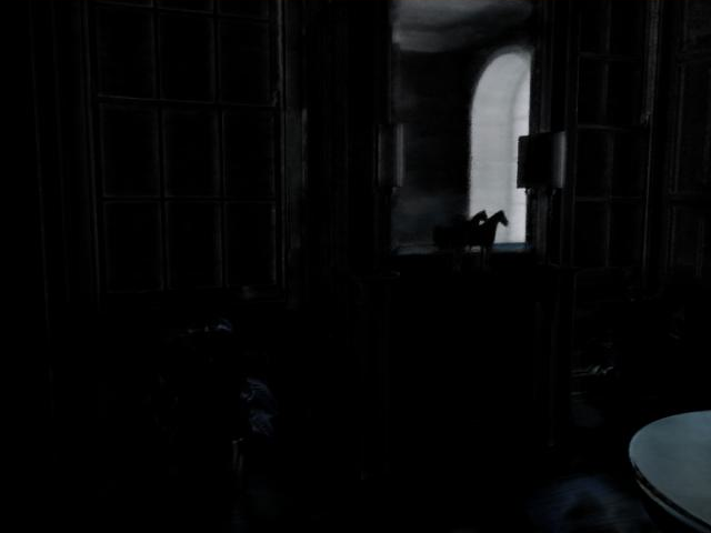
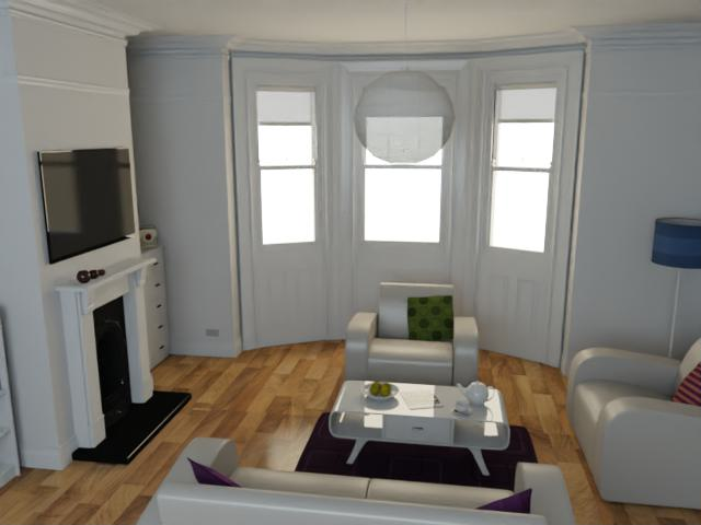
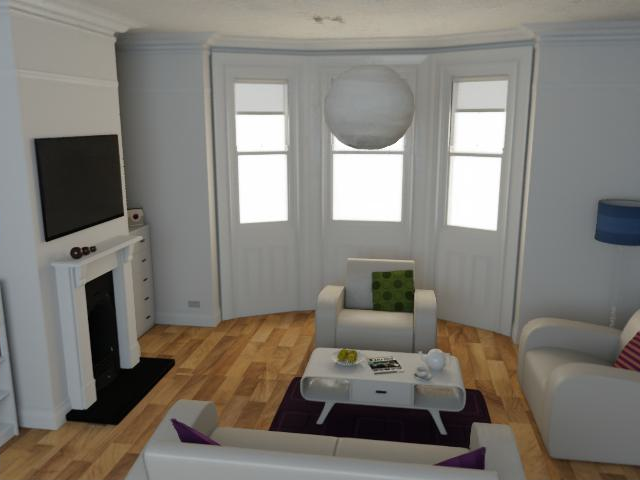
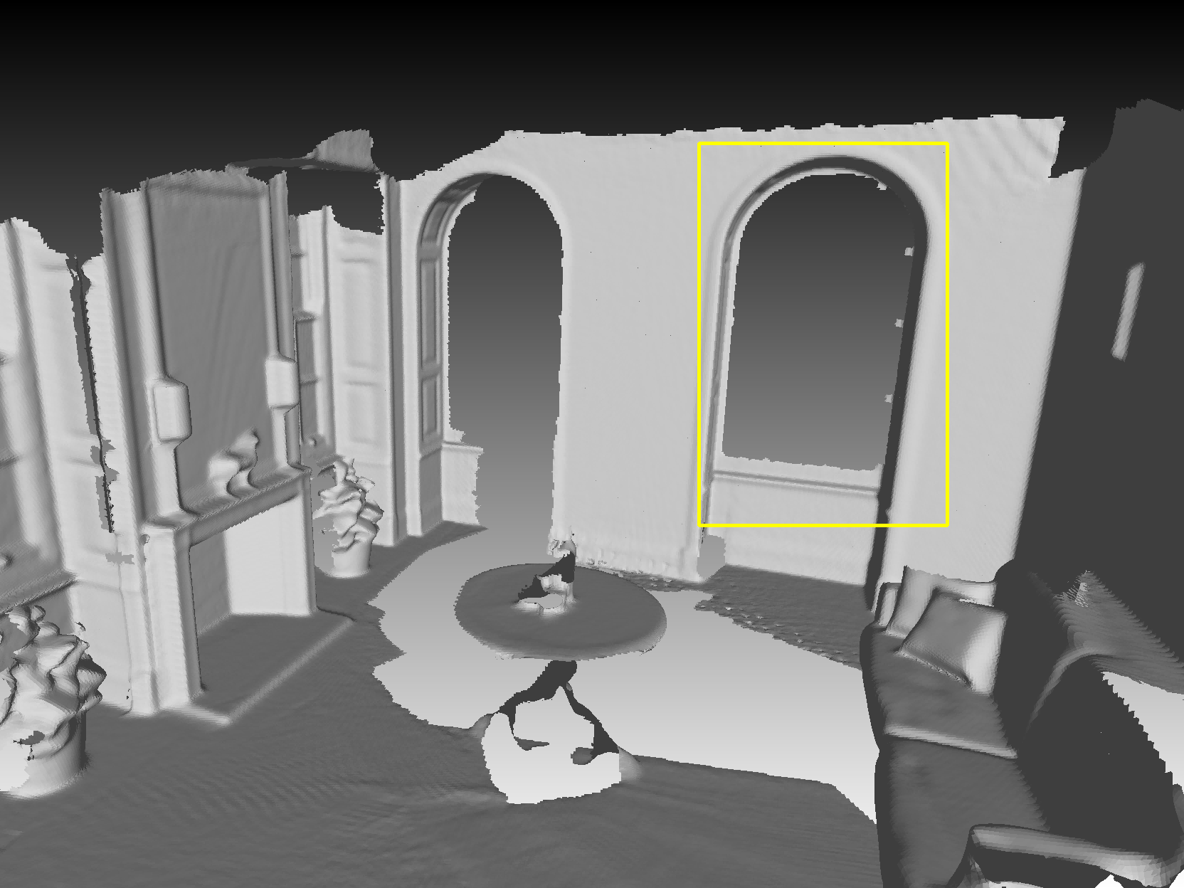
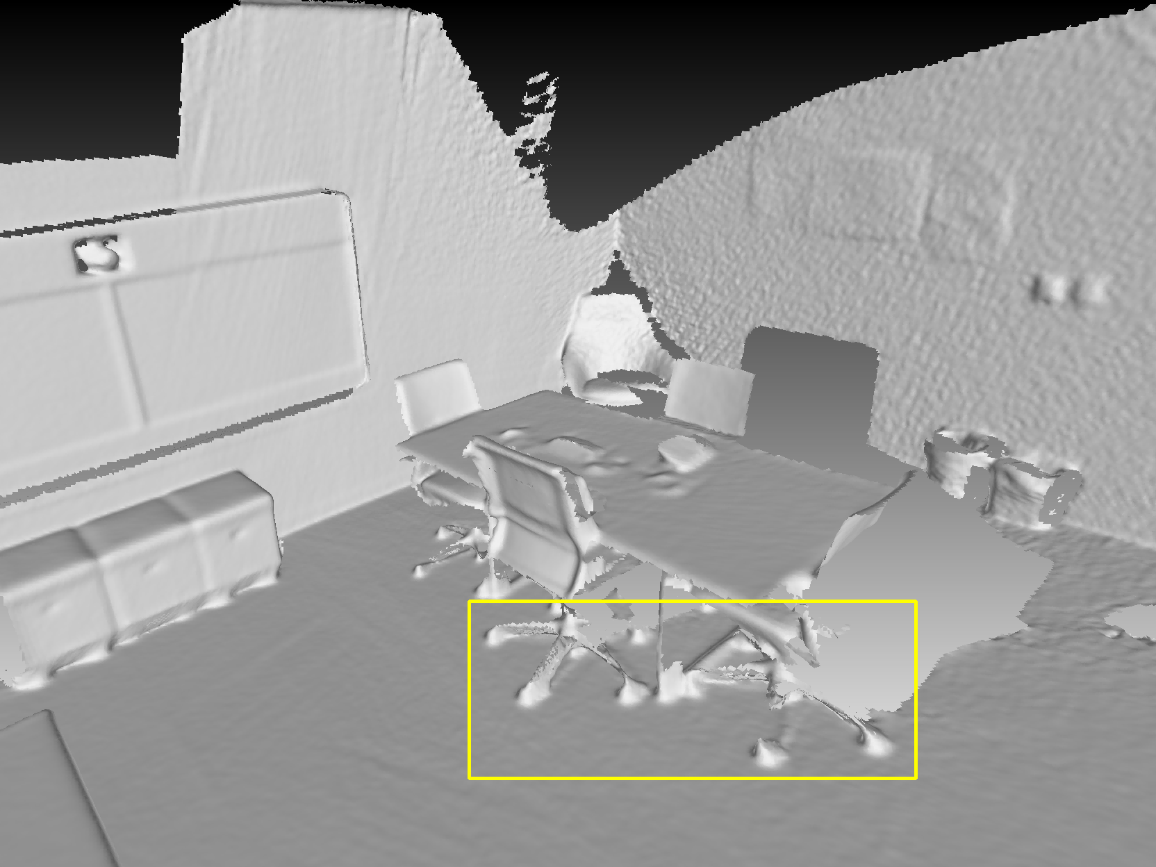
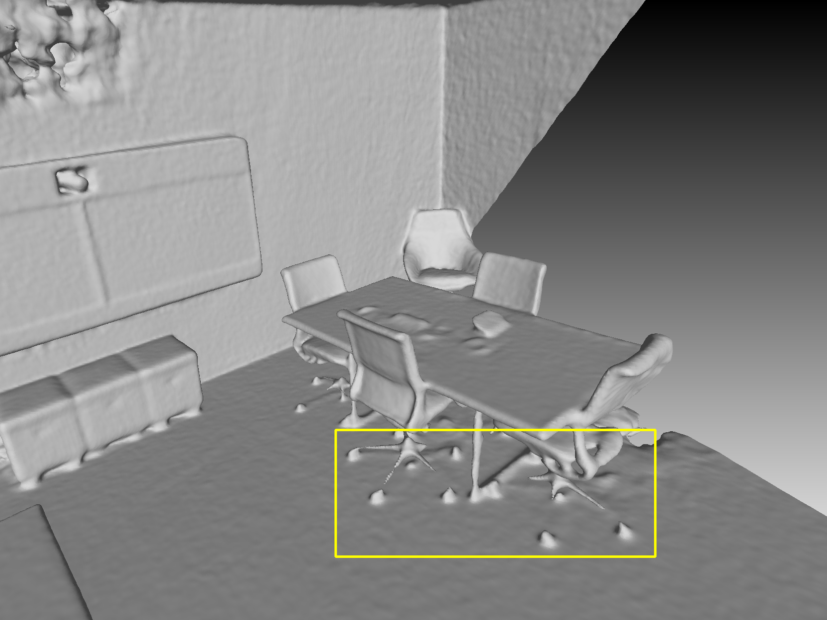
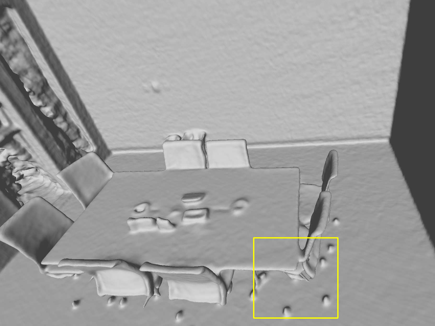
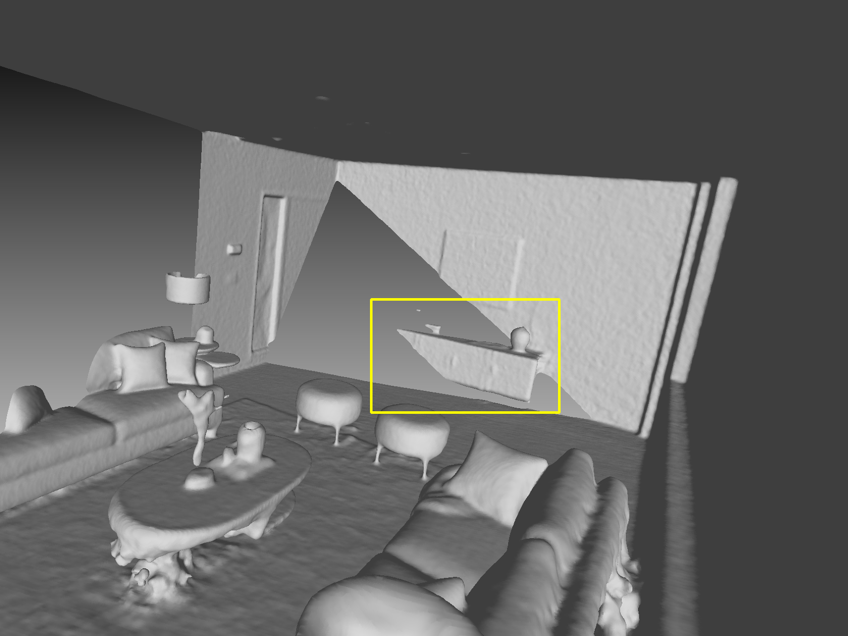
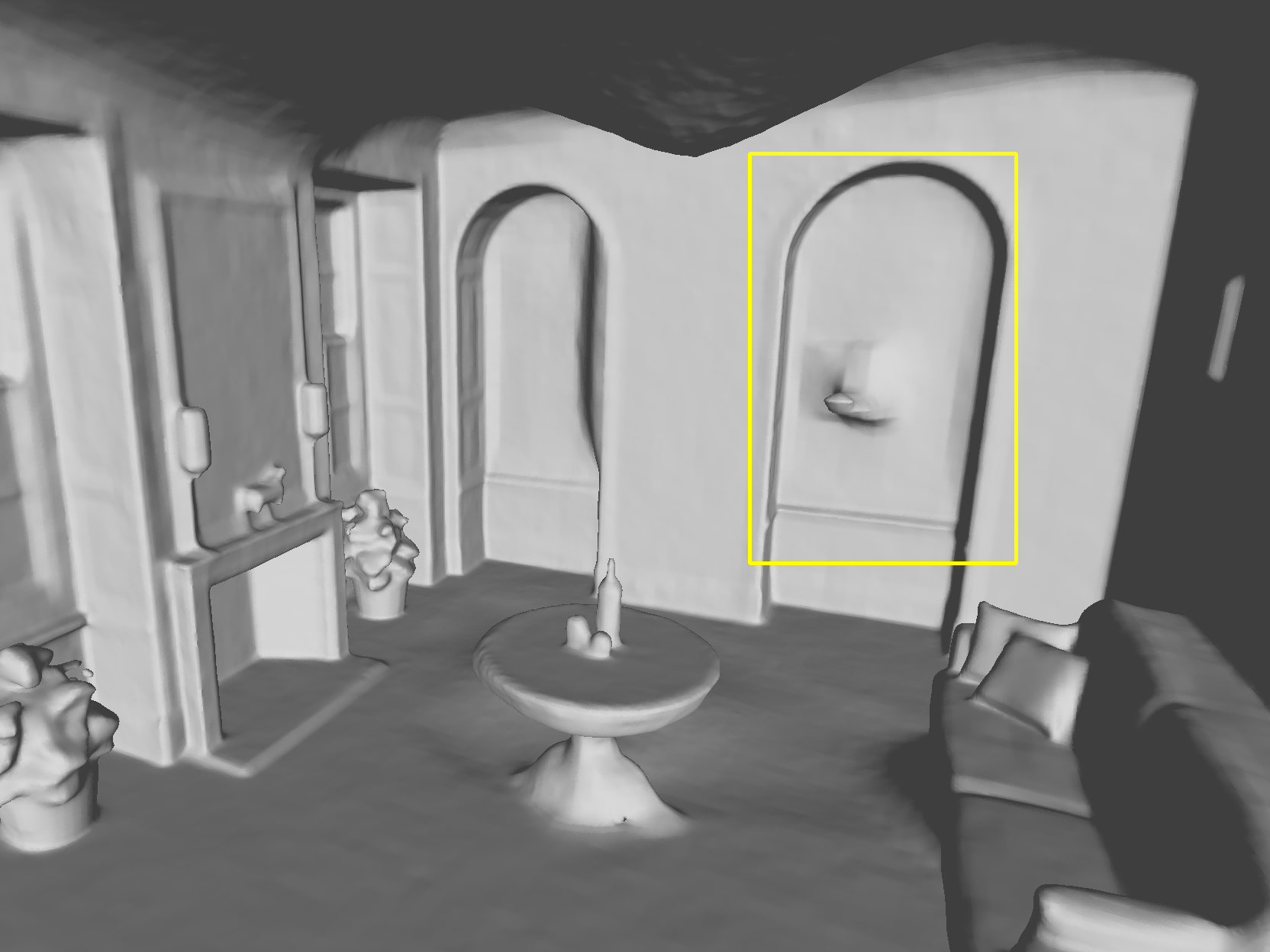
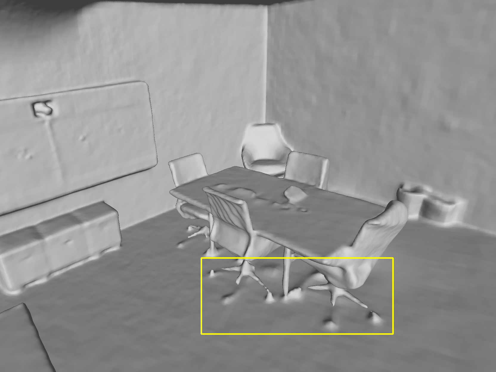
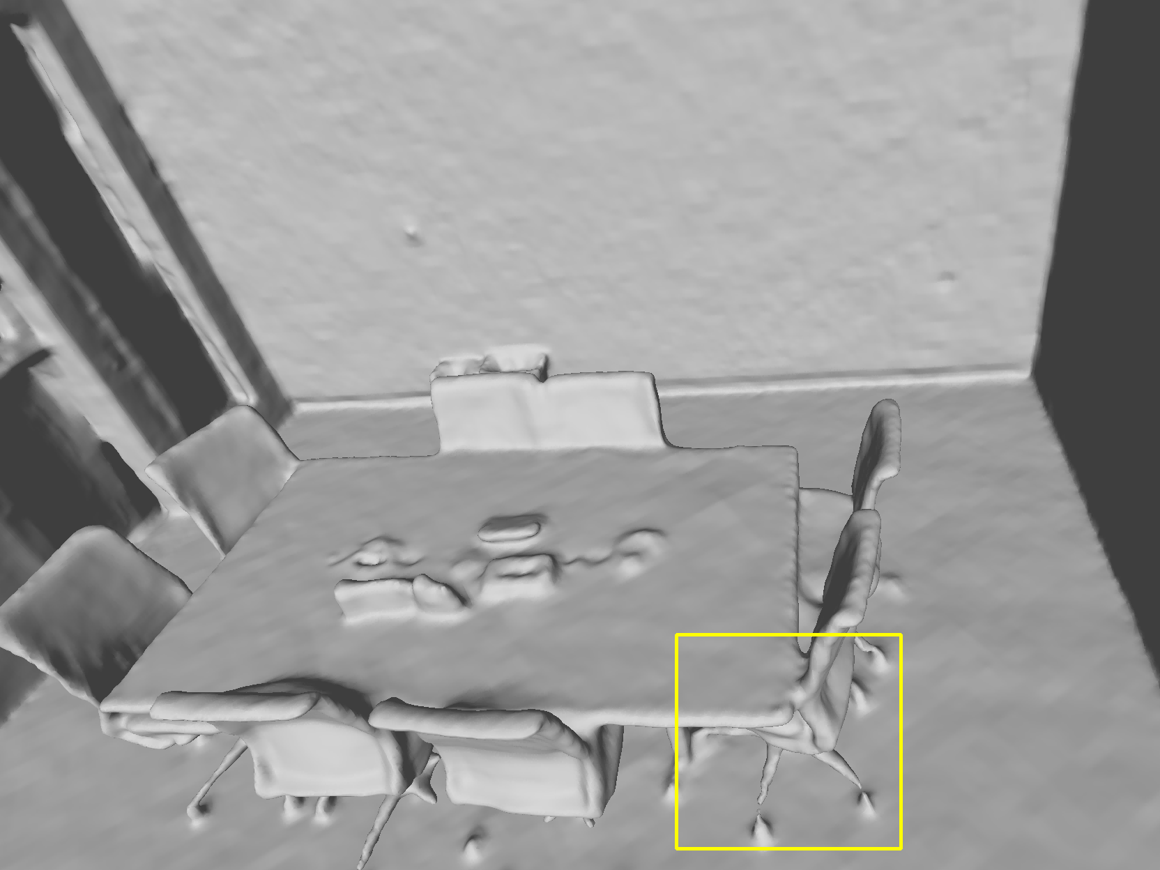
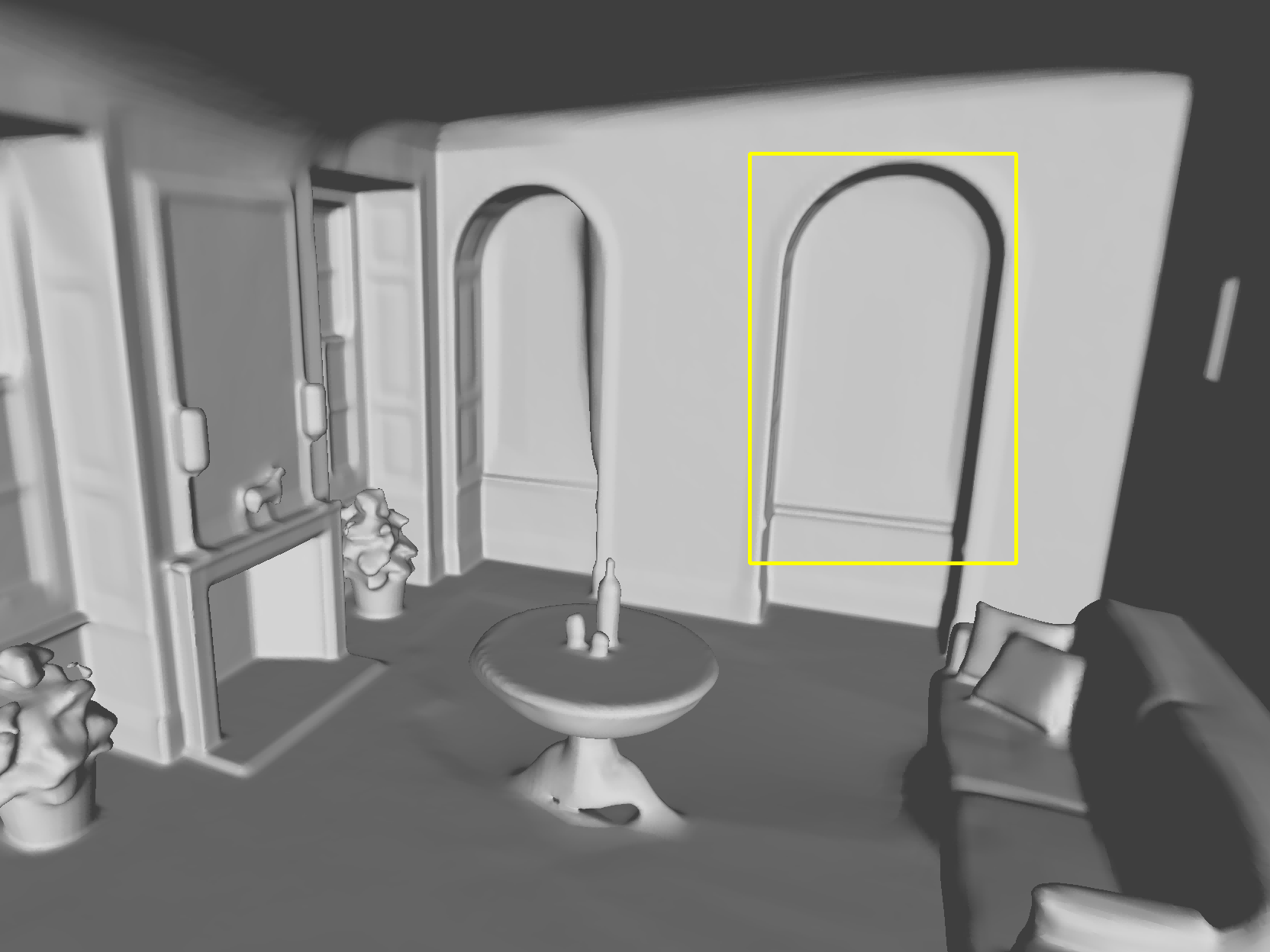
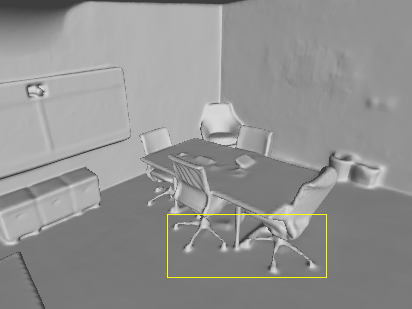
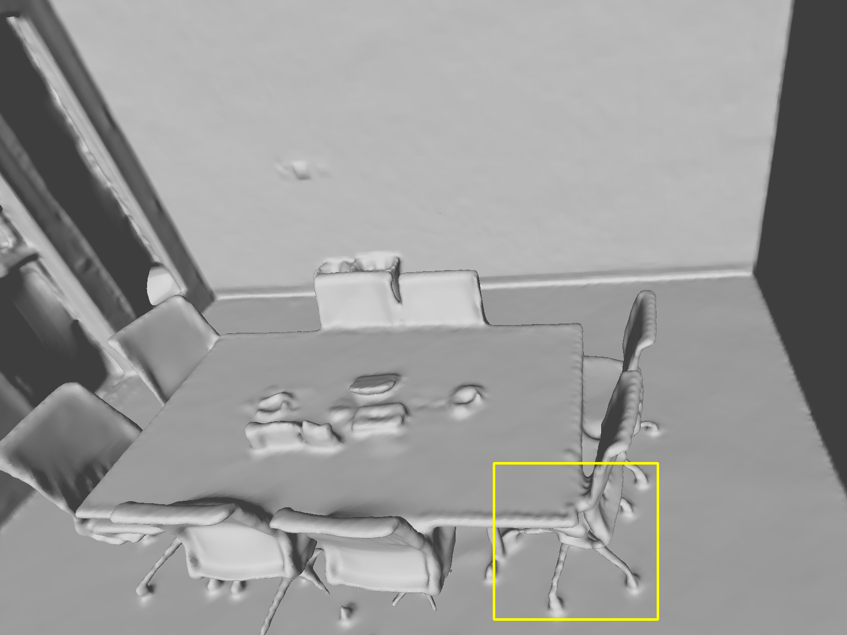
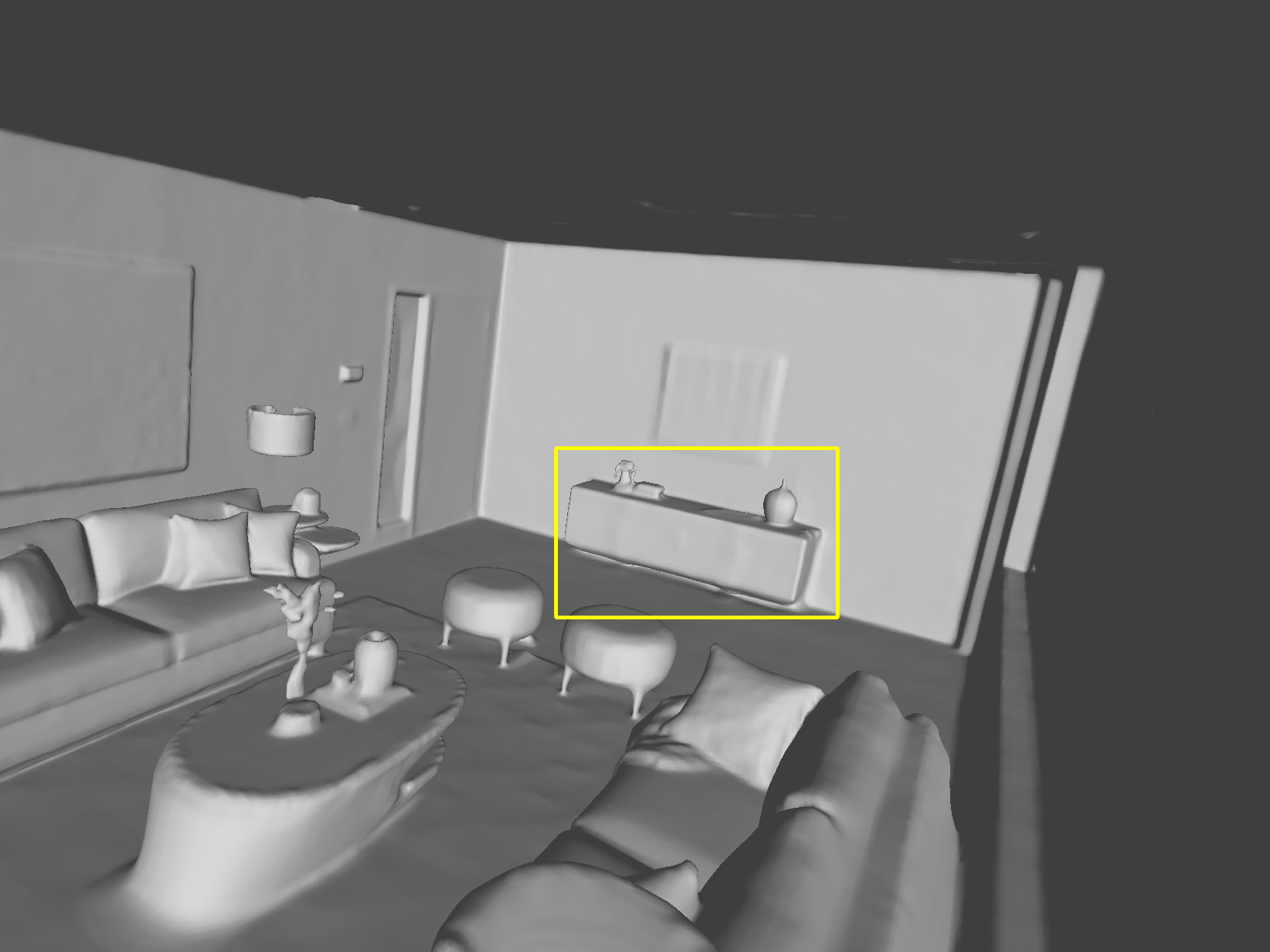
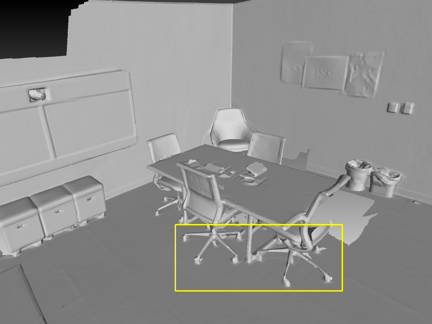
Qualitative and quantitative results are shown in Fig. 2 and Tab. 1. It can be seen from Tab. 1 that our method obtains the best performance on image rendering and indoor reconstruction compared with previous approaches. Specifically, we achieve the best performances in accuracy, completion, chamfer distance, and the highest F-score values. We also achieve the highest PSNR and SSIM and the lowest LPIPS. Additionally, Fig. 2 shows that our approach can fill in the missing parts of the scene in scene reconstruction, such as the legs of the chair and light strips. We also obtain smoother surfaces in flat areas such as the floor. In terms of view rendering, our approach exceeds rendering and reconstruction of previous approaches in reconstructing geometric features and achieves visually better images.






| Method | Acc | Com | C- | NC | F-score | PSNR | SSIM | LPIPS |
|---|---|---|---|---|---|---|---|---|
| BundleFusion | 0.0178 | 0.4577 | 0.2378 | 0.851 | 0.680 | - | - | - |
| COLMAP | 0.0271 | 0.0364 | 0.0293 | 0.888 | 0.874 | - | - | - |
| ConvOccNets | 0.0498 | 0.0524 | 0.0511 | 0.861 | 0.682 | - | - | - |
| SIREN | 0.0229 | 0.0412 | 0.0320 | 0.905 | 0.852 | - | - | - |
| Neus | 0.3174 | 0.6911 | 0.5043 | 0.628 | 0.103 | 27.465 | 0.849 | 0.192 |
| VolSDF | 0.1627 | 0.4815 | 0.3222 | 0.681 | 0.262 | 28.717 | 0.882 | 0.174 |
| Neural RGB-D | 0.0145 | 0.0508 | 0.0327 | 0.920 | 0.936 | 31.994 | 0.901 | 0.183 |
| Go-Surf | 0.0164 | 0.0213 | 0.0189 | 0.932 | 0.949 | 29.586 | 0.889 | 0.183 |
| DVGO | 0.2389 | 0.5558 | 0.3973 | 0.564 | 0.317 | 33.633 | 0.940 | 0.125 |
| Instant-NGP | 0.2641 | 0.7318 | 0.4976 | 0.555 | 0.208 | 27.976 | 0.799 | 0.255 |
| Ours | 0.0156 | 0.0197 | 0.0177 | 0.933 | 0.960 | 36.503 | 0.966 | 0.048 |
Evaluation on Replica dataset. The Replica dataset consists of 18 scenes, which are closer to real-world scenes. Each scene contains about 2000 high-quality images and depth images. We also add noise to their depth images, as in [1], to simulate real depth images [2, 5, 14]. Moreover, we also perform BundleFusion to produce the camera poses. We chose one image from every 10 images for the whole image sequence as the validation dataset. We empirically discard the first and last images as they capture scenes that the training dataset does not have.
It can be seen from table Tab. 2 that our method achieves the best performance on geometry reconstruction and view rendering. Specifically, for geometric reconstruction, the proposed method achieves better performance than traditional BundleFusion in all metrics. Moreover, we achieve higher F-score and lower chamfer- compared to NeuralRGBD and Go-Surf. In terms of view rendering, our method outperforms these methods by a large margin in all three metrics, even better than DVGO and Instant-NGP, which are designed for novel view synthesis. Qualitative results can be found in the supplementary material.
| Method | Acc | Com | C- | NC | F-score | PSNR | SSIM | LPIPS |
|---|---|---|---|---|---|---|---|---|
| BundleFusion | 0.0145 | 0.0453 | 0.0299 | 0.961 | 0.936 | - | - | - |
| Neus | 0.1623 | 0.2956 | 0.2288 | 0.754 | 0.194 | 28.939 | 0.855 | 0.181 |
| VolSDF | 0.1348 | 0.3009 | 0.2180 | 0.747 | 0.339 | 30.375 | 0.866 | 0.175 |
| Neural RGB-D | 0.0096 | 0.2447 | 0.1271 | 0.934 | 0.847 | 32.668 | 0.893 | 0.198 |
| Go-Surf | 0.0120 | 0.0122 | 0.0121 | 0.9718 | 0.9896 | 30.967 | 0.884 | 0.217 |
| DVGO | 0.2399 | 0.3511 | 0.2955 | 0.6040 | 0.239 | 31.962 | 0.893 | 0.223 |
| Instant-NGP | 0.3332 | 1.1151 | 0.7288 | 0.5470 | 0.1583 | 32.352 | 0.884 | 0.150 |
| Ours | 0.0112 | 0.0111 | 0.0112 | 0.9748 | 0.9911 | 37.104 | 0.955 | 0.074 |
Complexity and efficiency. The proposed method takes about 50 to 90 minutes on our hardware to obtain a high-quality rendering and reconstruction. This performance is slower than Go-Surf [44] (15-45 minutes) but way faster than Neural RGBD [1] (over 12 hours). The storage requirement of Du-NeRF is comparable to that of Go-surf which is in the order of hundreds of MB for storing two feature grids and other network parameters.
4.3 Ablations
We conduct ablation studies to demonstrate the effectiveness of designing the blocks and choice of scene representation. The quantitative result is shown in Tabs. 3, 4 and 5, where we evaluate these methods in the RGBD synthetic dataset.
Effect of the Du-NeRF architecture. As shown in Tab. 3, the dual field significantly improves the view rendering performance, and simultaneously increases reconstruction performance. The SDF-only in Tab. 3 means only the SDF branch used for neural volume rendering without the density branch, while the Density-only represents only the density branch without that of SDF. Dual field means that two branches are used for volume rendering at the same time, in which the final color comes from the density branch, and the geometry is extracted from the SDF branch. This demonstrates the effectiveness of the proposed dual-field structure in enhancing the view rendering and indoor 3D reconstruction.
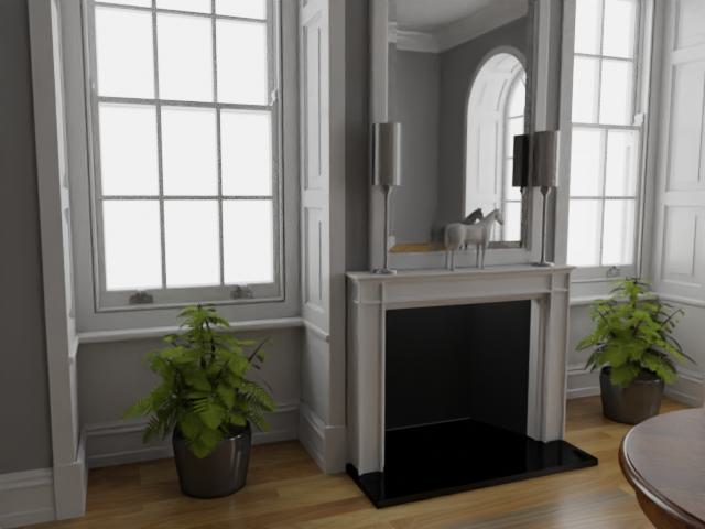
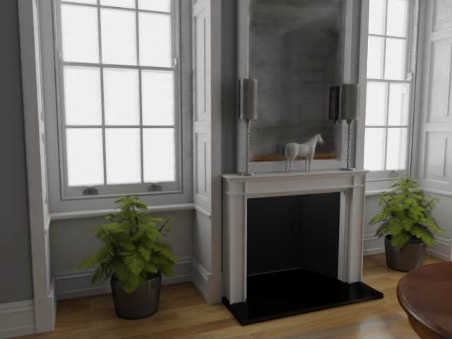
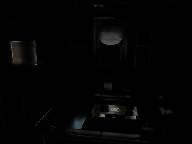
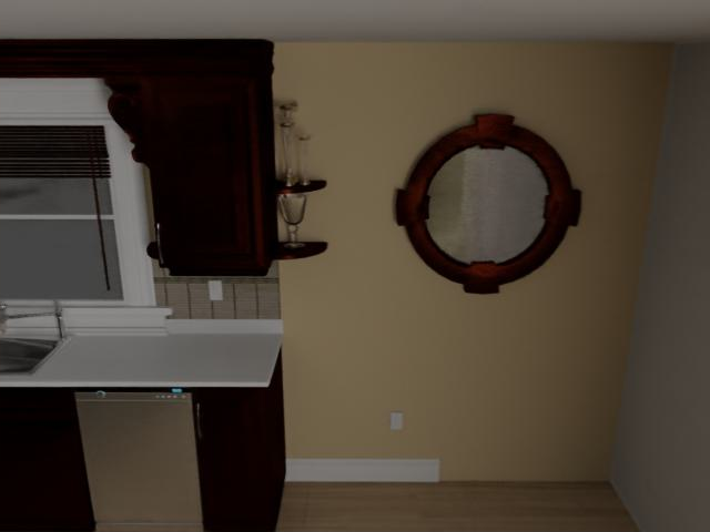
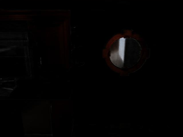
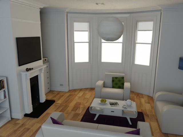
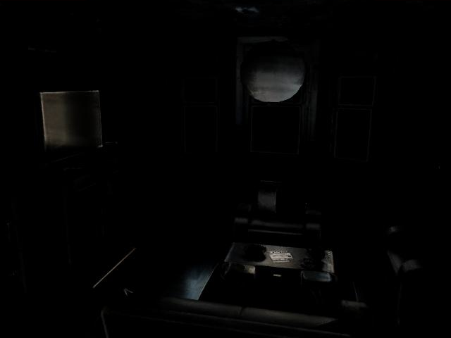
Effect of color disentanglement. Tab. 4 shows the ablation experiments of the color disentanglement (C-D). We tested the impact of different components of the color decoupling process on the final result, including the view-independent component (ViC), view-dependent component (VdC), and complete color (FC) is the sum of VdC and ViC. For the first row we use Fc instead of VdC+ViC due to color decoupling is not used in this experiment. It can be seen from the results that pure color decoupling cannot improve the quality of reconstruction and rendering from the first two rows. In addition, using ViC supervision to guide the learning of the SDF branch, the performance on F-score and PSNR are higher than other ways of supervision and the method without C-D, which confirms the effectiveness of our approach discussed in Sec. 3.2. The color decomposition results are shown in Fig. 4. It can be seen that the proposed method successfully decomposes the view-dependent color and view-independent color (see regions in the mirror, the reflective books, and the desk).
Effect of different grid representation. In Tab. 5, indicates the geometry and colour are both represented with four-level resolution grids, indicates the two are hash-based grid, and denotes the geometry is represented with a four-level grid while color is a hash-based grid. Tab. 5 shows that the hash representation of color features is helpful for obtaining better rendering performances while the hash representation of geometry features severely decreases the reconstruction quality.
| Method | C- | F-score | PSNR | LPIPS |
|---|---|---|---|---|
| SDF-only | 0.0203 | 0.9500 | 32.198 | 0.117 |
| Density-only | 0.0279 | 0.8798 | 31.681 | 0.155 |
| Dual(SDF+Density) | 0.0182 | 0.9549 | 34.494 | 0.090 |
| C-D | Supervised | C- | F-score | PSNR | LPIPS |
|---|---|---|---|---|---|
| w/o | FC | 0.0182 | 0.9549 | 34.494 | 0.090 |
| w/ | VdC+ViC | 0.0185 | 0.9526 | 34.710 | 0.080 |
| w/ | VdC | 0.1658 | 0.6503 | 32.780 | 0.122 |
| w/ | ViC | 0.0177 | 0.9597 | 35.225 | 0.072 |
| Method | C- | F-score | PSNR | LPIPS |
|---|---|---|---|---|
| 0.0177 | 0.9597 | 35.225 | 0.072 | |
| 0.0294 | 0.8976 | 36.087 | 0.108 | |
| 0.0177 | 0.9600 | 36.503 | 0.048 |
5 Concluding remarks
We have presented a dual neural radiance field for high-fidelity 3D scene reconstruction and rendering simultaneously. By designing two branches for reconstruction and view rendering respectively, the proposed method allows the two tasks to benefit from each other. To further improve the reconstruction and rendering performances, we designed a self-supervised color decomposition method. Experimental results have shown that our self-supervised method simultaneously improves the geometric reconstruction and rendering capabilities. Moreover, our method achieves state-of-the-art performances compared to previous methods.
Limitation and future work. Although Du-NeRF has been experimentally proven to be effective, our method may perform poorly if the observed images are blurred because it relies on multi-view color consistency to supervise geometry reconstruction and blur images do not satisfy such requirements. Besides, the effectiveness of the proposed method remains to be tested under a few-shot scenario where a small number of RGBD images are provided. In addition, trying new feature representations such as replacing hash representation with Gaussian splitting may improve performances. We will address these in future works.
References
- Azinović et al. [2022] Dejan Azinović, Ricardo Martin-Brualla, Dan B Goldman, Matthias Nießner, and Justus Thies. Neural rgb-d surface reconstruction. In Proceedings of the IEEE/CVF Conference on Computer Vision and Pattern Recognition, pages 6290–6301, 2022.
- Barron and Malik [2013] Jonathan T Barron and Jitendra Malik. Intrinsic scene properties from a single rgb-d image. In Proceedings of the IEEE Conference on Computer Vision and Pattern Recognition, pages 17–24, 2013.
- Barron et al. [2021] Jonathan T Barron, Ben Mildenhall, Matthew Tancik, Peter Hedman, Ricardo Martin-Brualla, and Pratul P Srinivasan. Mip-nerf: A multiscale representation for anti-aliasing neural radiance fields. In Proceedings of the IEEE/CVF International Conference on Computer Vision, pages 5855–5864, 2021.
- Bian et al. [2023] Wenjing Bian, Zirui Wang, Kejie Li, Jia-Wang Bian, and Victor Adrian Prisacariu. Nope-nerf: Optimising neural radiance field with no pose prior. In Proceedings of the IEEE/CVF Conference on Computer Vision and Pattern Recognition, pages 4160–4169, 2023.
- Bohg et al. [2014] Jeannette Bohg, Javier Romero, Alexander Herzog, and Stefan Schaal. Robot arm pose estimation through pixel-wise part classification. In 2014 IEEE International Conference on Robotics and Automation (ICRA), pages 3143–3150. IEEE, 2014.
- Chen et al. [2022] Anpei Chen, Zexiang Xu, Andreas Geiger, Jingyi Yu, and Hao Su. Tensorf: Tensorial radiance fields. In Computer Vision – ECCV 2022, pages 333–350. 2022.
- Chen et al. [2013] Jiawen Chen, Dennis Bautembach, and Shahram Izadi. Scalable real-time volumetric surface reconstruction. ACM Transactions on Graphics (ToG), 32(4):1–16, 2013.
- Chen and Lee [2023] Yu Chen and Gim Hee Lee. Dbarf: Deep bundle-adjusting generalizable neural radiance fields. In Proceedings of the IEEE/CVF Conference on Computer Vision and Pattern Recognition, pages 24–34, 2023.
- Curless and Levoy [1996] Brian Curless and Marc Levoy. A volumetric method for building complex models from range images. In Proceedings of the 23rd annual conference on Computer graphics and interactive techniques, pages 303–312, 1996.
- Dai et al. [2017] Angela Dai, Matthias Nießner, Michael Zollhöfer, Shahram Izadi, and Christian Theobalt. Bundlefusion: Real-time globally consistent 3d reconstruction using on-the-fly surface reintegration. ACM Transactions on Graphics (ToG), 36(4):1, 2017.
- Fridovich-Keil et al. [2022] Sara Fridovich-Keil, Alex Yu, Matthew Tancik, Qinhong Chen, Benjamin Recht, and Angjoo Kanazawa. Plenoxels: Radiance fields without neural networks. In Proceedings of the IEEE/CVF Conference on Computer Vision and Pattern Recognition, pages 5501–5510, 2022.
- Godard et al. [2017] Clément Godard, Oisin Mac Aodha, and Gabriel J Brostow. Unsupervised monocular depth estimation with left-right consistency. In Proceedings of the IEEE conference on computer vision and pattern recognition, pages 270–279, 2017.
- Guo et al. [2022] Haoyu Guo, Sida Peng, Haotong Lin, Qianqian Wang, Guofeng Zhang, Hujun Bao, and Xiaowei Zhou. Neural 3d scene reconstruction with the manhattan-world assumption. In Proceedings of the IEEE/CVF Conference on Computer Vision and Pattern Recognition, pages 5511–5520, 2022.
- Handa et al. [2014] Ankur Handa, Thomas Whelan, John McDonald, and Andrew J Davison. A benchmark for rgb-d visual odometry, 3d reconstruction and slam. In 2014 IEEE international conference on Robotics and automation (ICRA), pages 1524–1531. IEEE, 2014.
- Izadi et al. [2011] Shahram Izadi, David Kim, Otmar Hilliges, David Molyneaux, Richard Newcombe, Pushmeet Kohli, Jamie Shotton, Steve Hodges, Dustin Freeman, Andrew Davison, et al. Kinectfusion: real-time 3d reconstruction and interaction using a moving depth camera. In Proceedings of the 24th annual ACM symposium on User interface software and technology, pages 559–568, 2011.
- Kang et al. [2023] Xujie Kang, Kanglin Liu, Jiang Duan, Yuanhao Gong, and Guoping Qiu. P2i-net: Mapping camera pose to image via adversarial learning for new view synthesis in real indoor environments. page 2635–2643, 2023.
- Kar et al. [2017] Abhishek Kar, Christian Häne, and Jitendra Malik. Learning a multi-view stereo machine. Advances in neural information processing systems, 30, 2017.
- Kerbl et al. [2023] Bernhard Kerbl, Georgios Kopanas, Thomas Leimkühler, and George Drettakis. 3d gaussian splatting for real-time radiance field rendering. ACM Transactions on Graphics (ToG), 42(4):1–14, 2023.
- Kwon et al. [2023] Obin Kwon, Jeongho Park, and Songhwai Oh. Renderable neural radiance map for visual navigation. In Proceedings of the IEEE/CVF Conference on Computer Vision and Pattern Recognition, pages 9099–9108, 2023.
- Lee et al. [2023a] Dogyoon Lee, Minhyeok Lee, Chajin Shin, and Sangyoun Lee. Dp-nerf: Deblurred neural radiance field with physical scene priors. In Proceedings of the IEEE/CVF Conference on Computer Vision and Pattern Recognition, pages 12386–12396, 2023a.
- Lee et al. [2023b] Seunghwan Lee, Gwanmo Park, Hyewon Son, Jiwon Ryu, and Han Joo Chae. Fastsurf: Fast neural rgb-d surface reconstruction using per-frame intrinsic refinement and tsdf fusion prior learning. arXiv preprint arXiv:2303.04508, 2023b.
- Li et al. [2023] Zhaoshuo Li, Thomas Müller, Alex Evans, Russell H Taylor, Mathias Unberath, Ming-Yu Liu, and Chen-Hsuan Lin. Neuralangelo: High-fidelity neural surface reconstruction. In Proceedings of the IEEE/CVF Conference on Computer Vision and Pattern Recognition, pages 8456–8465, 2023.
- Liu et al. [2020] Lingjie Liu, Jiatao Gu, Kyaw Zaw Lin, Tat-Seng Chua, and Christian Theobalt. Neural sparse voxel fields. Advances in Neural Information Processing Systems, 33:15651–15663, 2020.
- Max [1995] Nelson Max. Optical models for direct volume rendering. IEEE Transactions on Visualization and Computer Graphics, 1(2):99–108, 1995.
- Mescheder et al. [2019] Lars Mescheder, Michael Oechsle, Michael Niemeyer, Sebastian Nowozin, and Andreas Geiger. Occupancy networks: Learning 3d reconstruction in function space. In Proceedings of the IEEE/CVF conference on computer vision and pattern recognition, pages 4460–4470, 2019.
- Mildenhall et al. [2020] B Mildenhall, PP Srinivasan, M Tancik, JT Barron, R Ramamoorthi, and R Ng. Nerf: Representing scenes as neural radiance fields for view synthesis. In European conference on computer vision, 2020.
- Müller et al. [2022] Thomas Müller, Alex Evans, Christoph Schied, and Alexander Keller. Instant neural graphics primitives with a multiresolution hash encoding. ACM Transactions on Graphics, 41(4):1–15, 2022.
- Nießner et al. [2013] Matthias Nießner, Michael Zollhöfer, Shahram Izadi, and Marc Stamminger. Real-time 3d reconstruction at scale using voxel hashing. ACM Transactions on Graphics (ToG), 32(6):1–11, 2013.
- Oechsle et al. [2019] Michael Oechsle, Lars Mescheder, Michael Niemeyer, Thilo Strauss, and Andreas Geiger. Texture fields: Learning texture representations in function space. In Proceedings of the IEEE/CVF International Conference on Computer Vision, pages 4531–4540, 2019.
- Oechsle et al. [2021] Michael Oechsle, Songyou Peng, and Andreas Geiger. Unisurf: Unifying neural implicit surfaces and radiance fields for multi-view reconstruction. In Proceedings of the IEEE/CVF International Conference on Computer Vision, pages 5589–5599, 2021.
- Park et al. [2019] Jeong Joon Park, Peter Florence, Julian Straub, Richard Newcombe, and Steven Lovegrove. Deepsdf: Learning continuous signed distance functions for shape representation. In Proceedings of the IEEE/CVF conference on computer vision and pattern recognition, pages 165–174, 2019.
- Peng et al. [2020] Songyou Peng, Michael Niemeyer, Lars Mescheder, Marc Pollefeys, and Andreas Geiger. Convolutional occupancy networks. In Computer Vision–ECCV 2020: 16th European Conference, Glasgow, UK, August 23–28, 2020, Proceedings, Part III 16, pages 523–540. Springer, 2020.
- Reiser et al. [2023] Christian Reiser, Rick Szeliski, Dor Verbin, Pratul Srinivasan, Ben Mildenhall, Andreas Geiger, Jon Barron, and Peter Hedman. Merf: Memory-efficient radiance fields for real-time view synthesis in unbounded scenes. ACM Transactions on Graphics (TOG), 42(4):1–12, 2023.
- Schonberger and Frahm [2016] Johannes L Schonberger and Jan-Michael Frahm. Structure-from-motion revisited. In Proceedings of the IEEE conference on computer vision and pattern recognition, pages 4104–4113, 2016.
- Schönberger et al. [2016] Johannes L Schönberger, Enliang Zheng, Jan-Michael Frahm, and Marc Pollefeys. Pixelwise view selection for unstructured multi-view stereo. In Computer Vision–ECCV 2016: 14th European Conference, Amsterdam, The Netherlands, October 11-14, 2016, Proceedings, Part III 14, pages 501–518. Springer, 2016.
- Schönberger et al. [2017] Johannes L Schönberger, True Price, Torsten Sattler, Jan-Michael Frahm, and Marc Pollefeys. A vote-and-verify strategy for fast spatial verification in image retrieval. In Computer Vision–ACCV 2016: 13th Asian Conference on Computer Vision, Taipei, Taiwan, November 20-24, 2016, Revised Selected Papers, Part I 13, pages 321–337. Springer, 2017.
- Sitzmann et al. [2019a] Vincent Sitzmann, Justus Thies, Felix Heide, Matthias Nießner, Gordon Wetzstein, and Michael Zollhofer. Deepvoxels: Learning persistent 3d feature embeddings. In Proceedings of the IEEE/CVF Conference on Computer Vision and Pattern Recognition, pages 2437–2446, 2019a.
- Sitzmann et al. [2019b] Vincent Sitzmann, Michael Zollhöfer, and Gordon Wetzstein. Scene representation networks: Continuous 3d-structure-aware neural scene representations. Advances in Neural Information Processing Systems, 32, 2019b.
- Sitzmann et al. [2020] Vincent Sitzmann, Julien Martel, Alexander Bergman, David Lindell, and Gordon Wetzstein. Implicit neural representations with periodic activation functions. Advances in neural information processing systems, 33:7462–7473, 2020.
- Sun et al. [2022] Cheng Sun, Min Sun, and Hwann-Tzong Chen. Direct voxel grid optimization: Super-fast convergence for radiance fields reconstruction. In Proceedings of the IEEE/CVF Conference on Computer Vision and Pattern Recognition, pages 5459–5469, 2022.
- Tancik et al. [2023] Matthew Tancik, Ethan Weber, Evonne Ng, Ruilong Li, Brent Yi, Justin Kerr, Terrance Wang, Alexander Kristoffersen, Jake Austin, Kamyar Salahi, Abhik Ahuja, David McAllister, and Angjoo Kanazawa. Nerfstudio: A modular framework for neural radiance field development. In ACM SIGGRAPH 2023 Conference Proceedings, 2023.
- Tang et al. [2023] Jiaxiang Tang, Hang Zhou, Xiaokang Chen, Tianshu Hu, Errui Ding, Jingdong Wang, and Gang Zeng. Delicate textured mesh recovery from nerf via adaptive surface refinement. arXiv preprint arXiv:2303.02091, 2023.
- Tatarchenko et al. [2017] Maxim Tatarchenko, Alexey Dosovitskiy, and Thomas Brox. Octree generating networks: Efficient convolutional architectures for high-resolution 3d outputs. In Proceedings of the IEEE international conference on computer vision, pages 2088–2096, 2017.
- Wang et al. [2022] Jingwen Wang, Tymoteusz Bleja, and Lourdes Agapito. Go-surf: Neural feature grid optimization for fast, high-fidelity rgb-d surface reconstruction. In 2022 International Conference on 3D Vision (3DV), pages 433–442. IEEE, 2022.
- Wang et al. [2021] Peng Wang, Lingjie Liu, Yuan Liu, Christian Theobalt, Taku Komura, and Wenping Wang. Neus: Learning neural implicit surfaces by volume rendering for multi-view reconstruction. arXiv preprint arXiv:2106.10689, 2021.
- Wang et al. [2023] Peng Wang, Yuan Liu, Zhaoxi Chen, Lingjie Liu, Ziwei Liu, Taku Komura, Christian Theobalt, and Wenping Wang. F2-nerf: Fast neural radiance field training with free camera trajectories. In Proceedings of the IEEE/CVF Conference on Computer Vision and Pattern Recognition, pages 4150–4159, 2023.
- Xu et al. [2023] Xiangyu Xu, Lichang Chen, Changjiang Cai, Huangying Zhan, Qingan Yan, Pan Ji, Junsong Yuan, Heng Huang, and Yi Xu. Dynamic voxel grid optimization for high-fidelity rgb-d supervised surface reconstruction. arXiv preprint arXiv:2304.06178, 2023.
- Yao et al. [2018] Yao Yao, Zixin Luo, Shiwei Li, Tian Fang, and Long Quan. Mvsnet: Depth inference for unstructured multi-view stereo. In Proceedings of the European conference on computer vision (ECCV), pages 767–783, 2018.
- Yariv et al. [2021] Lior Yariv, Jiatao Gu, Yoni Kasten, and Yaron Lipman. Volume rendering of neural implicit surfaces. Advances in Neural Information Processing Systems, 34:4805–4815, 2021.
- Yu et al. [2021] Alex Yu, Ruilong Li, Matthew Tancik, Hao Li, Ren Ng, and Angjoo Kanazawa. Plenoctrees for real-time rendering of neural radiance fields. In Proceedings of the IEEE/CVF International Conference on Computer Vision, pages 5752–5761, 2021.
- Yu et al. [2022a] Zehao Yu, Anpei Chen, Bozidar Antic, Songyou Peng, Apratim Bhattacharyya, Michael Niemeyer, Siyu Tang, Torsten Sattler, and Andreas Geiger. Sdfstudio: A unified framework for surface reconstruction, 2022a.
- Yu et al. [2022b] Zehao Yu, Songyou Peng, Michael Niemeyer, Torsten Sattler, and Andreas Geiger. Monosdf: Exploring monocular geometric cues for neural implicit surface reconstruction. Advances in neural information processing systems, 35:25018–25032, 2022b.
- Zhang et al. [2020] Kai Zhang, Gernot Riegler, Noah Snavely, and Vladlen Koltun. Nerf++: Analyzing and improving neural radiance fields. arXiv preprint arXiv:2010.07492, 2020.
- Zhou et al. [2023] Kun Zhou, Wenbo Li, Yi Wang, Tao Hu, Nianjuan Jiang, Xiaoguang Han, and Jiangbo Lu. Nerflix: High-quality neural view synthesis by learning a degradation-driven inter-viewpoint mixer. In Proceedings of the IEEE/CVF Conference on Computer Vision and Pattern Recognition, pages 12363–12374, 2023.
- Zhu et al. [2023] Bingfan Zhu, Yanchao Yang, Xulong Wang, Youyi Zheng, and Leonidas Guibas. Vdn-nerf: Resolving shape-radiance ambiguity via view-dependence normalization. In Proceedings of the IEEE/CVF Conference on Computer Vision and Pattern Recognition, pages 35–45, 2023.
- Zollhöfer et al. [2018] Michael Zollhöfer, Patrick Stotko, Andreas Görlitz, Christian Theobalt, Matthias Nießner, Reinhard Klein, and Andreas Kolb. State of the art on 3d reconstruction with rgb-d cameras. In Computer graphics forum, pages 625–652. Wiley Online Library, 2018.
Supplementary Material
6 Additional Implementation Details
6.1 More details of the dataset
We use the NeuralRGBD and the Replica datasets to evaluate the proposed method. The NeuralRGBD contains ten synthetic scenes and the Replica has eight real-world scenes. Each scene consists of RGB images, depth images (coarse, real) and poses (coarse, real).
We use the coarse depth images and poses for all experiments. The coarse depth images are made by adding noise to real depth images to simulate depth images obtained by the real depth sensor as in [2, 5, 14], and the coarse poses are estimated by BundleFusion using noisy depth images. For each scene, about 10 percent of images are used as validation sets and the rest of the images are used as training sets. Specifically, starting with the -th image, we choose one image in every ten consecutive images as the validation set. The details of the number of datasets are shown in Tab. 6.
6.2 More details of the scene representation
We use two different multi-resolution grids to store the hidden features for geometry and appearance reconstruction, including a four-level grid for geometry features and a hash-based grid for color features. Specifically, we determine the bounding box of the scene based on the GT mesh and set the voxel sizes of each level as 3cm, 6cm, 24cm and 96cm, respectively. We store 4-dim feature vectors for each resolution grid, and a 16-dim geometric feature vector is finally obtained. In addition, the setting of the hash-based grid, is identical with InstantNGP, including a levels hash table. The coarsest level has 16 grids and the finest has . Each level interpolates a feature vector of dimension 2, obtaining a total of a 32-dimensional feature vector. The spatial hash function used is the same as InstantNGP:
| (19) |
where T represents the maximum number of entries per level and the largest T is set to . The denotes the bitwise exclusive OR operation, and signifies distinctive, sizable prime numbers.
The coordinates of the scenes are normalized to . The SDFs are initialized in a ball shape, which allows for filling in the empty windows smoothly and speeding up the convergence.
| Scene | Frames | Train | Validate |
|---|---|---|---|
| Breakfast room | 1167 | 1051 | 116 |
| Green room | 1440 | 1297 | 143 |
| Grey-white room | 1490 | 1342 | 148 |
| ICL living room | 1445 | 1301 | 144 |
| Complete kitchen | 1210 | 1090 | 120 |
| Kitchen | 1184 | 1066 | 118 |
| Morning apartment | 920 | 829 | 91 |
| Staircase | 1118 | 1007 | 111 |
| Thin Geometry | 395 | 356 | 39 |
| White room | 1676 | 1509 | 167 |
| Office0 | 2000 | 1801 | 199 |
| Office1 | 2000 | 1801 | 199 |
| Office2 | 1997 | 1798 | 199 |
| Office3 | 1963 | 1767 | 196 |
| Office4 | 1968 | 1772 | 196 |
| Room0 | 1985 | 1787 | 198 |
| Room1 | 1996 | 1797 | 199 |
| Room2 | 1978 | 1781 | 197 |
6.3 More details of the framework
There are four decoders in the proposed framework including the SDF decoder, density decoder, color decoder and specular decoder. Each decoder is comprised of a two-layer MLP with hidden neurons of 32. The SDF decoder and density decoder share the input with the inputting features of dimension 16 while the color decoder takes as input color feature with dimension 32. The color decoder outputs a 3-dimensional vector denoting a view-independent color and a 32-dimensional feature. The 32-dimensional feature is concatenated with the view embedding feature and subsequently fed into the specular decoder. The view embedding feature is generated via four-level Fourier position encoding for the view direction, as done in the original NeRF, with a dimension of 27. The specular decoder takes the concatenated feature as input and outputs view-dependent color. The learning rate for all decoders is set to and the decay factor is set to at 10000 and 15000 iterations.
6.4 More details of the SDF loss functions
In order to robustly train the SDF decoder, we imposed a series of SDF losses (as shown in Eq. 20) to regularize the network as in [44]:
| (20) |
Loss is computed with Eq. 21. It calculates the distance between predicted SDF values and the real ones computed from depth value via , where is the ground truth of depth in pixel , and is the distance between sampling points to the camera centre.
| (21) |
Loss is used to encourage free space prediction instead of the fixed truncation values. It is computed with Eq. 22. Exponential penalty term equal to as in [44]. is zero when the SDF of a query point is positive and a large value if it is negative.
| (22) |
The regularization term encourages valid SDF predictions in unsupervised regions:
| (23) |
An explicit smoothness term is also added, named , where is randomly sampled from surface-proximal points and is a small offset in random directions set between 4mm and 1mm as in [44].
| (24) |
Empirical results demonstrate that the above constraints increase the robustness of the training SDF process.
| C- | F-score | PSNR | LPIPS | |
|---|---|---|---|---|
| 0.0132 | 0.985 | 36.926 | 0.0344 | |
| 0.0134 | 0.985 | 37.076 | 0.0353 | |
| (Ours) | 0.0128 | 0.985 | 37.167 | 0.0324 |
| 0.0132 | 0.985 | 37.146 | 0.0332 | |
| 0.0131 | 0.985 | 36.713 | 0.0359 |
| Method | C- | F-score | PSNR | LPIPS |
|---|---|---|---|---|
| Uϕ (Shared Grid) | 0.0123 | 0.972 | 29.917 | 0.150 |
| Sϕ (Double Grids) | 0.0115 | 0.976 | 31.741 | 0.110 |
| Uσ (Shared Grid) | 0.0195 | 0.982 | 32.644 | 0.094 |
| Sσ (Double Grids) | 0.0168 | 0.986 | 32.744 | 0.090 |
| Methods | Evaluation | office0 | office1 | office2 | office3 | office4 | room0 | room1 | room2 | Mean |
|---|---|---|---|---|---|---|---|---|---|---|
| BundleFusion | C- | 0.0109 | 0.0110 | 0.0310 | 0.0660 | 0.0165 | 0.0587 | 0.0110 | 0.0339 | 0.0299 |
| F-score | 0.9880 | 0.9910 | 0.9190 | 0.8410 | 0.9690 | 0.8820 | 0.9900 | 0.9100 | 0.9360 | |
| PSNR | - | - | - | - | - | - | - | - | - | |
| LPIPS | - | - | - | - | - | - | - | - | - | |
| Neus | C- | 0.0154 | 0.2280 | 0.2390 | 0.2000 | 0.3440 | 0.2140 | 0.1570 | 0.2940 | 0.2288 |
| F-score | 0.2340 | 0.1800 | 0.1730 | 0.3050 | 0.0850 | 0.2300 | 0.2210 | 0.1240 | 0.1940 | |
| PSNR | 33.274 | 33.874 | 26.372 | 26.893 | 28.546 | 25.913 | 28.068 | 28.570 | 28.939 | |
| LPIPS | 0.1570 | 0.1240 | 0.1790 | 0.1640 | 0.1660 | 0.2660 | 0.2120 | 0.1790 | 0.1810 | |
| VolSDF | C- | 0.1270 | 0.2050 | 0.1820 | 0.2830 | 0.2980 | 0.2750 | 0.1580 | 0.2160 | 0.2180 |
| F-score | 0.4200 | 0.2440 | 0.4150 | 0.3250 | 0.2980 | 0.3280 | 0.3810 | 0.3010 | 0.3390 | |
| PSNR | 34.327 | 35.733 | 28.996 | 27.943 | 30.595 | 26.374 | 28.807 | 30.227 | 30.375 | |
| LPIPS | 0.1570 | 0.1120 | 0.1650 | 0.1730 | 0.1590 | 0.2660 | 0.2140 | 0.1560 | 0.1750 | |
| NeuralRGBD | C- | 0.0635 | 0.0088 | 0.0544 | 0.0177 | 0.3340 | 0.0892 | 0.1010 | 0.3480 | 0.1271 |
| F-score | 0.8550 | 0.9890 | 0.9380 | 0.9790 | 0.7040 | 0.8740 | 0.8420 | 0.5960 | 0.8470 | |
| PSNR | 36.563 | 38.148 | 31.559 | 30.509 | 33.934 | 28.311 | 30.866 | 31.452 | 32.668 | |
| LPIPS | 0.1640 | 0.1590 | 0.2000 | 0.1840 | 0.1600 | 0.2750 | 0.2410 | 0.2000 | 0.1980 | |
| GO-Surf | C- | 0.0099 | 0.0104 | 0.0125 | 0.0156 | 0.0133 | 0.0131 | 0.0103 | 0.0117 | 0.0121 |
| F-score | 0.9880 | 0.9925 | 0.9875 | 0.9825 | 0.9890 | 0.9935 | 0.9960 | 0.9880 | 0.9896 | |
| PSNR | 35.105 | 35.655 | 29.059 | 29.138 | 31.784 | 27.378 | 29.522 | 30.096 | 30.967 | |
| LPIPS | 0.1620 | 0.1740 | 0.2355 | 0.1940 | 0.1835 | 0.2975 | 0.2650 | 0.2270 | 0.2170 | |
| InstantNGP | C- | 0.2560 | 1.2320 | 0.4940 | 0.4940 | 1.1500 | 0.7870 | 0.6270 | 0.7900 | 0.7288 |
| F-score | 0.2010 | 0.1020 | 0.2660 | 0.2660 | 0.1030 | 0.1050 | 0.1510 | 0.0720 | 0.1583 | |
| PSNR | 36.667 | 37.679 | 30.793 | 30.793 | 32.772 | 26.912 | 30.786 | 32.411 | 32.352 | |
| LPIPS | 0.1710 | 0.0754 | 0.1240 | 0.1240 | 0.2140 | 0.2620 | 0.1350 | 0.0976 | 0.1500 | |
| DVGO | C- | 0.2160 | 0.2790 | 0.2010 | 0.3270 | 0.3660 | 0.4160 | 0.2470 | 0.3120 | 0.2955 |
| F-score | 0.3170 | 0.2040 | 0.3010 | 0.2470 | 0.1330 | 0.2360 | 0.2630 | 0.2110 | 0.2390 | |
| PSNR | 36.859 | 37.878 | 31.596 | 28.349 | 32.583 | 26.985 | 30.250 | 31.192 | 31.962 | |
| LPIPS | 0.1670 | 0.1640 | 0.2100 | 0.2260 | 0.2100 | 0.3500 | 0.2510 | 0.2090 | 0.2230 | |
| Du-NeRF | C- | 0.0096 | 0.0102 | 0.0116 | 0.0141 | 0.0118 | 0.0119 | 0.0093 | 0.0108 | 0.0112 |
| F-score | 0.9890 | 0.9930 | 0.9900 | 0.9860 | 0.9910 | 0.9950 | 0.9970 | 0.9880 | 0.9911 | |
| PSNR | 41.365 | 41.922 | 34.913 | 34.622 | 37.776 | 34.184 | 36.123 | 35.928 | 37.104 | |
| LPIPS | 0.0546 | 0.0630 | 0.0933 | 0.0790 | 0.0775 | 0.0824 | 0.0673 | 0.0790 | 0.0740 |
7 Additional Ablation Study
The effect of the depth alignment. We conduct experiments to verify the importance of to color decomposition. The first row and second row shown in Fig. 5 represent the experiments w/o and w/ , respectively. It can be seen that the depth images predicted by the model without are blur and the process of the color decomposition fails. With the constraint of depth alignment, the view-independent component could be extracted correctly.
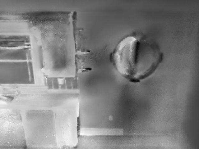
w/o
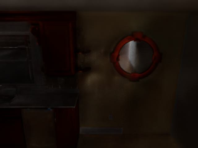
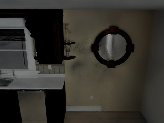
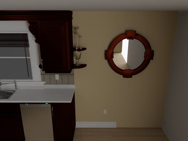
w/
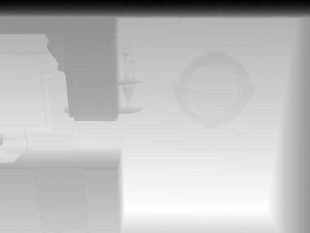

The effect of . The is very important for balancing the effect of color supervision and depth supervision. Smaller results in enhancing the effect of the depth loss and reducing the effect of the view-independent color supervision. Larger increases the effect of color supervision and decreases the effect of depth supervision. We carry out experiments with the different values of ranging from 0.5 to 50. The results in Tab. 7 show that gives the best performance. In addition, the performance drops whenever is larger or smaller.
The effect of separate color and geometry representation. We design a set of experiments to validate that separate representation of color and geometry using two different feature grids gives better results than that represented by the shared one. We conducted four experiments on the “morning apartment” scene for the indoor reconstruction and view synthesis. In Tab. 8, “U” indicates the experiment with the shared grid, and “S” represents the experiment of separate grids. represents the experiment that is supervised with color generated by SDF field. denotes the experiment that is supervised with color generated by density field. These results show that the separate representation of the geometry field and color field provides better performance on indoor reconstruction and view synthesis under both SDF color supervision and density color supervision.
8 Additional Experimental Results
8.1 More results on two indoor datasets
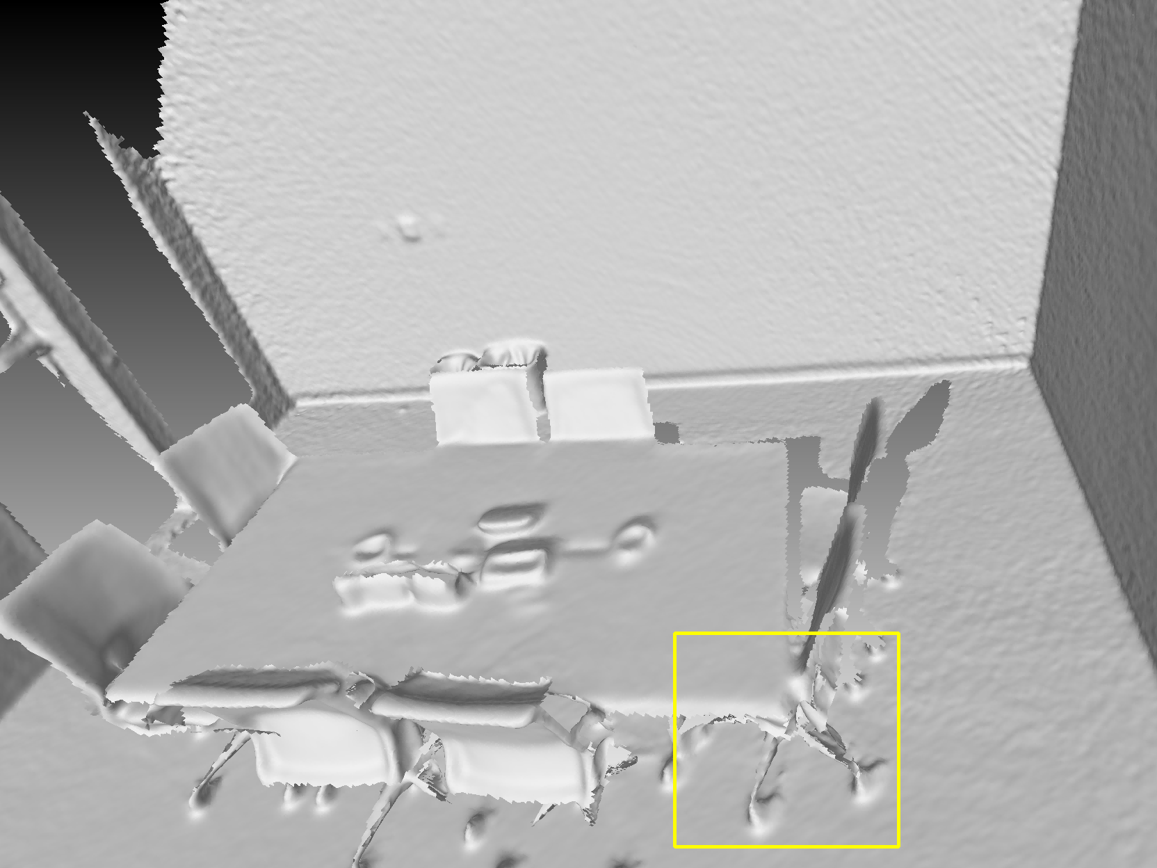
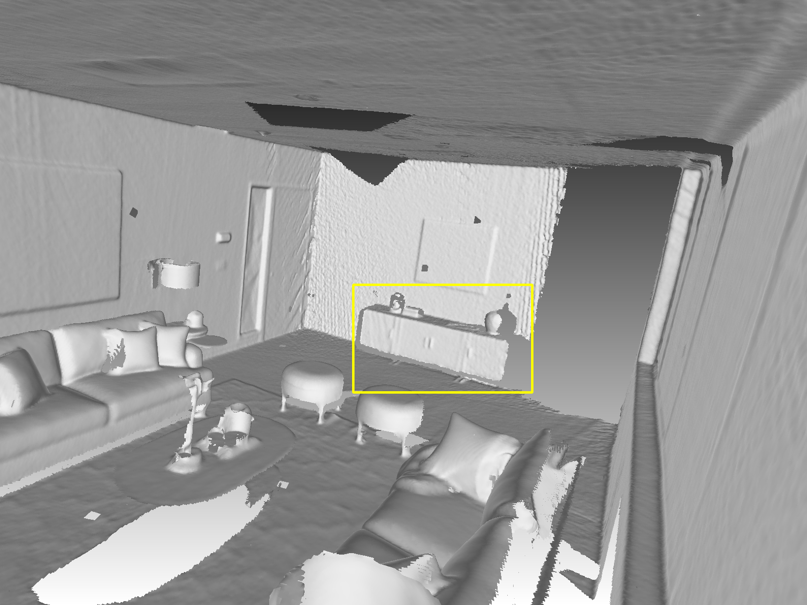
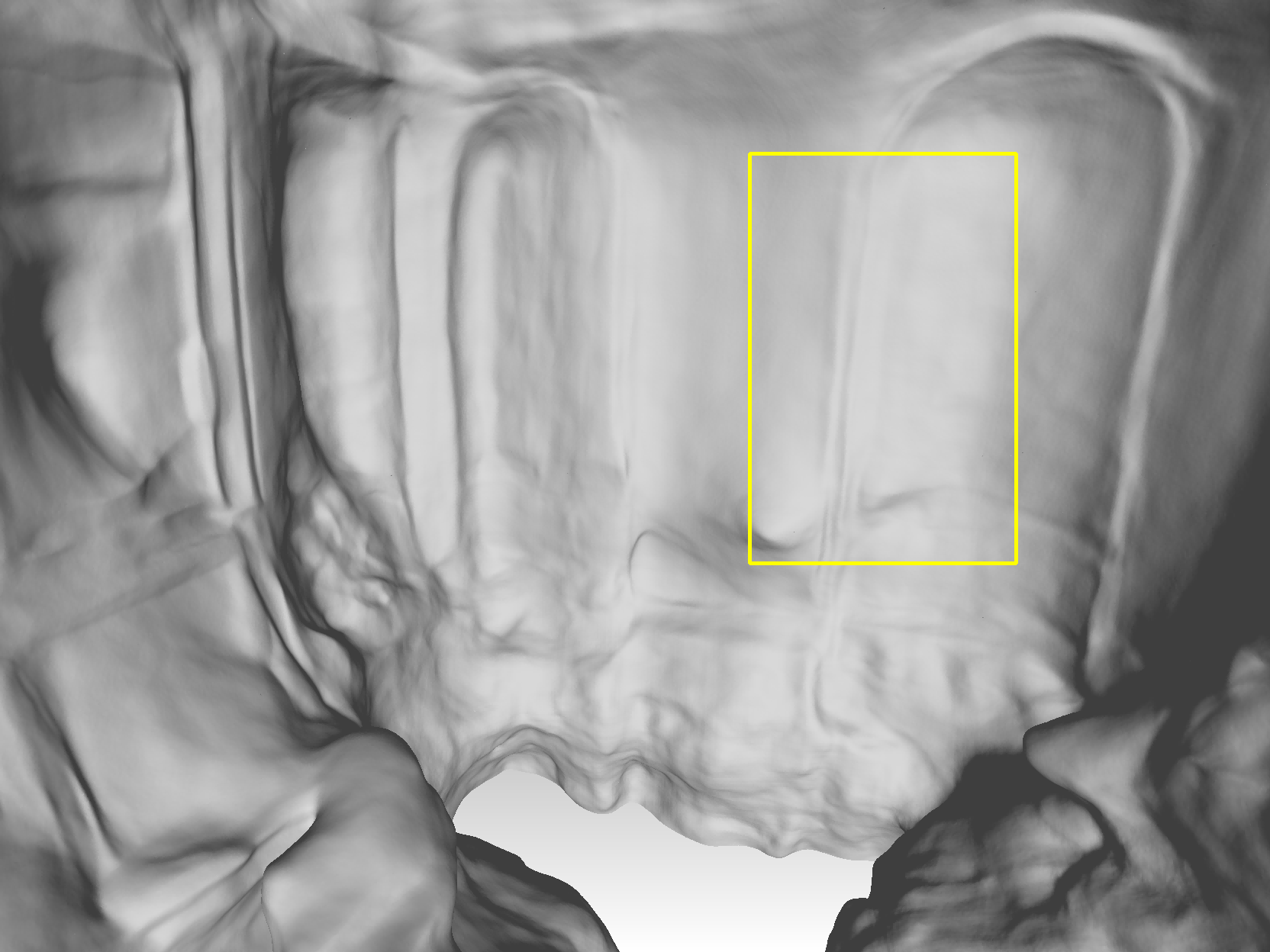
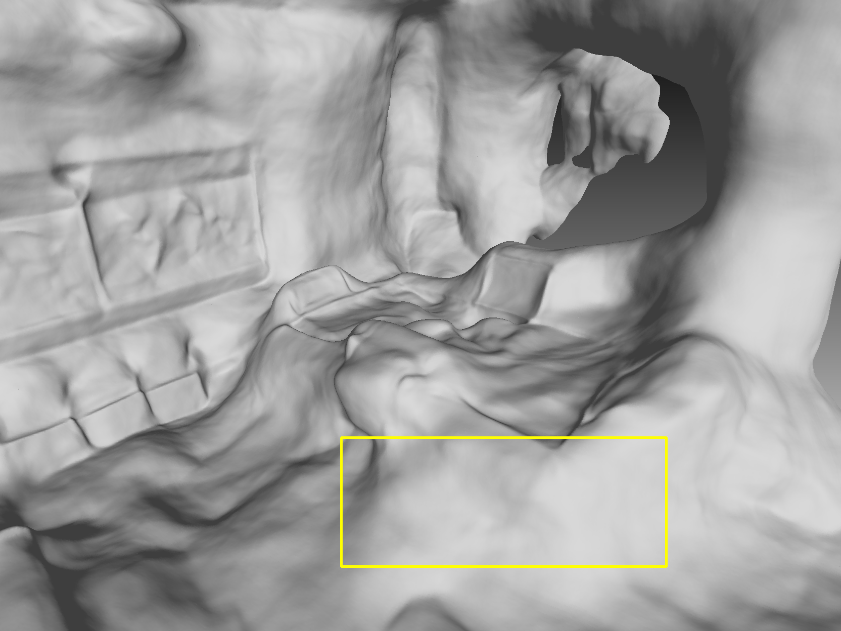
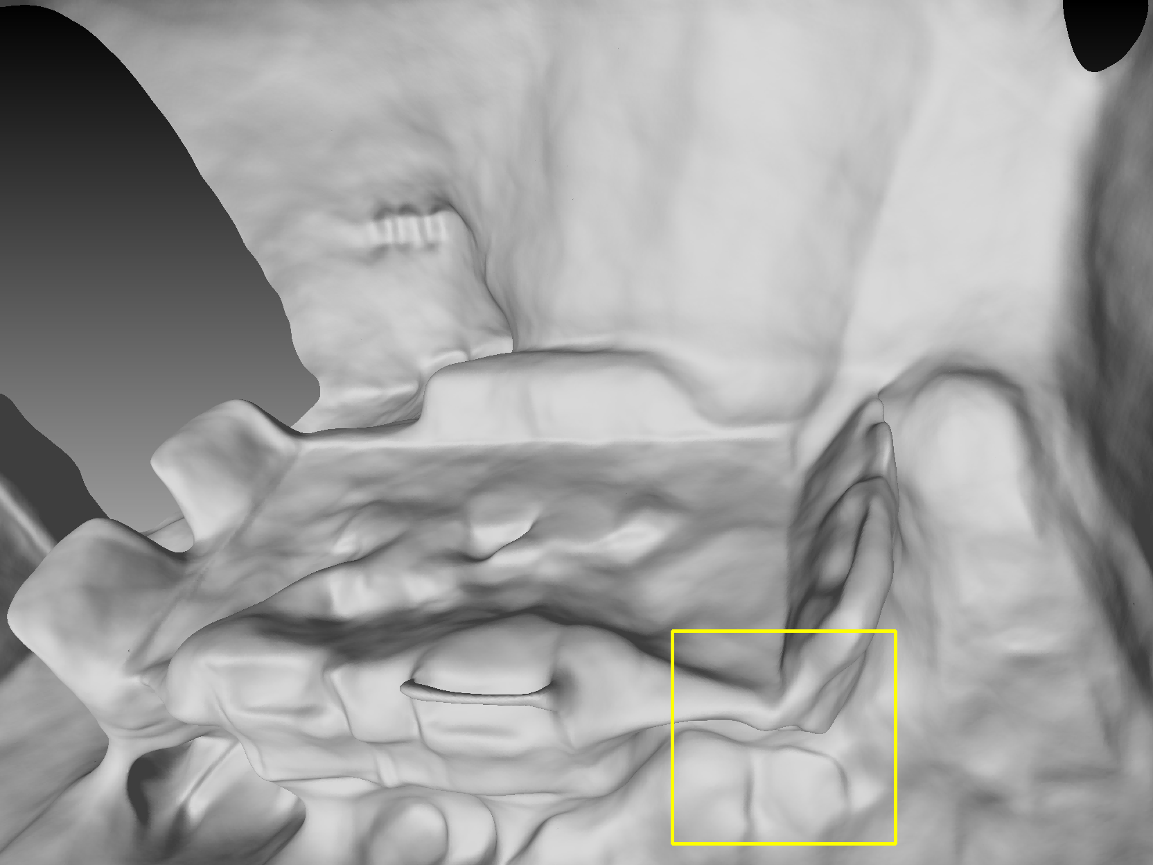
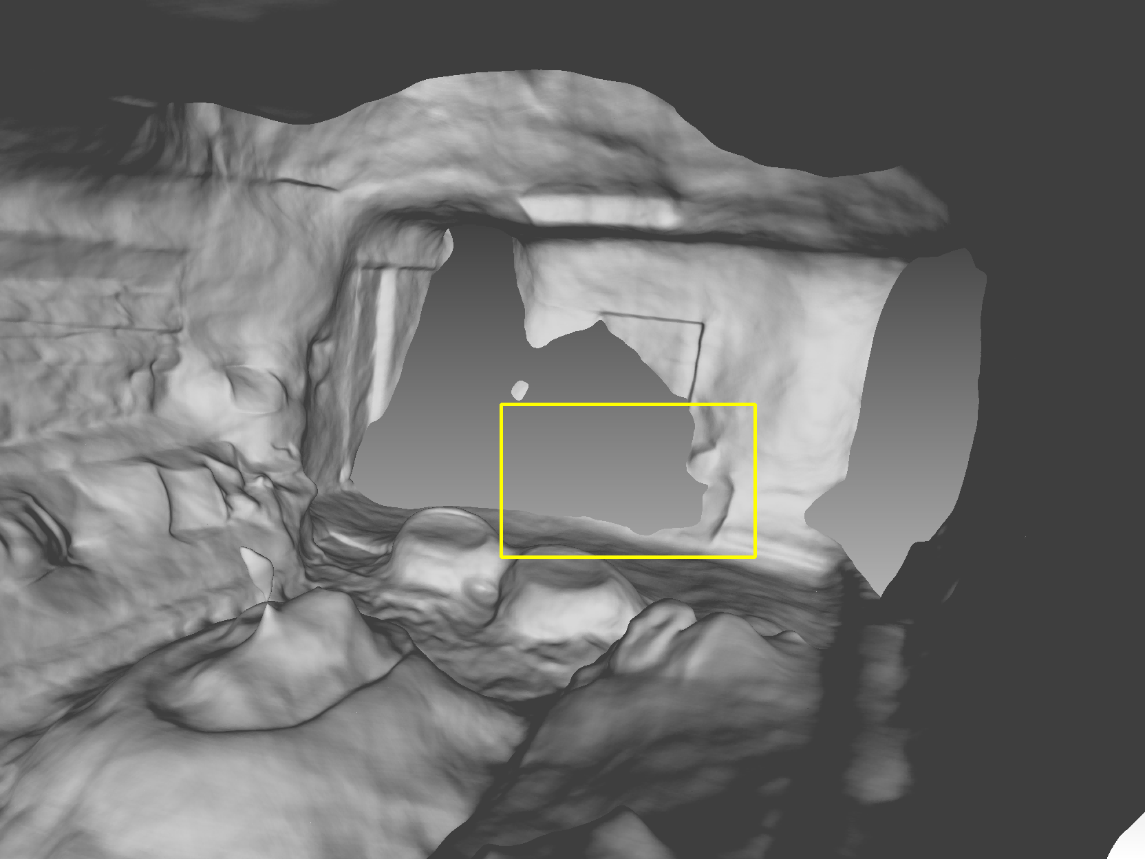
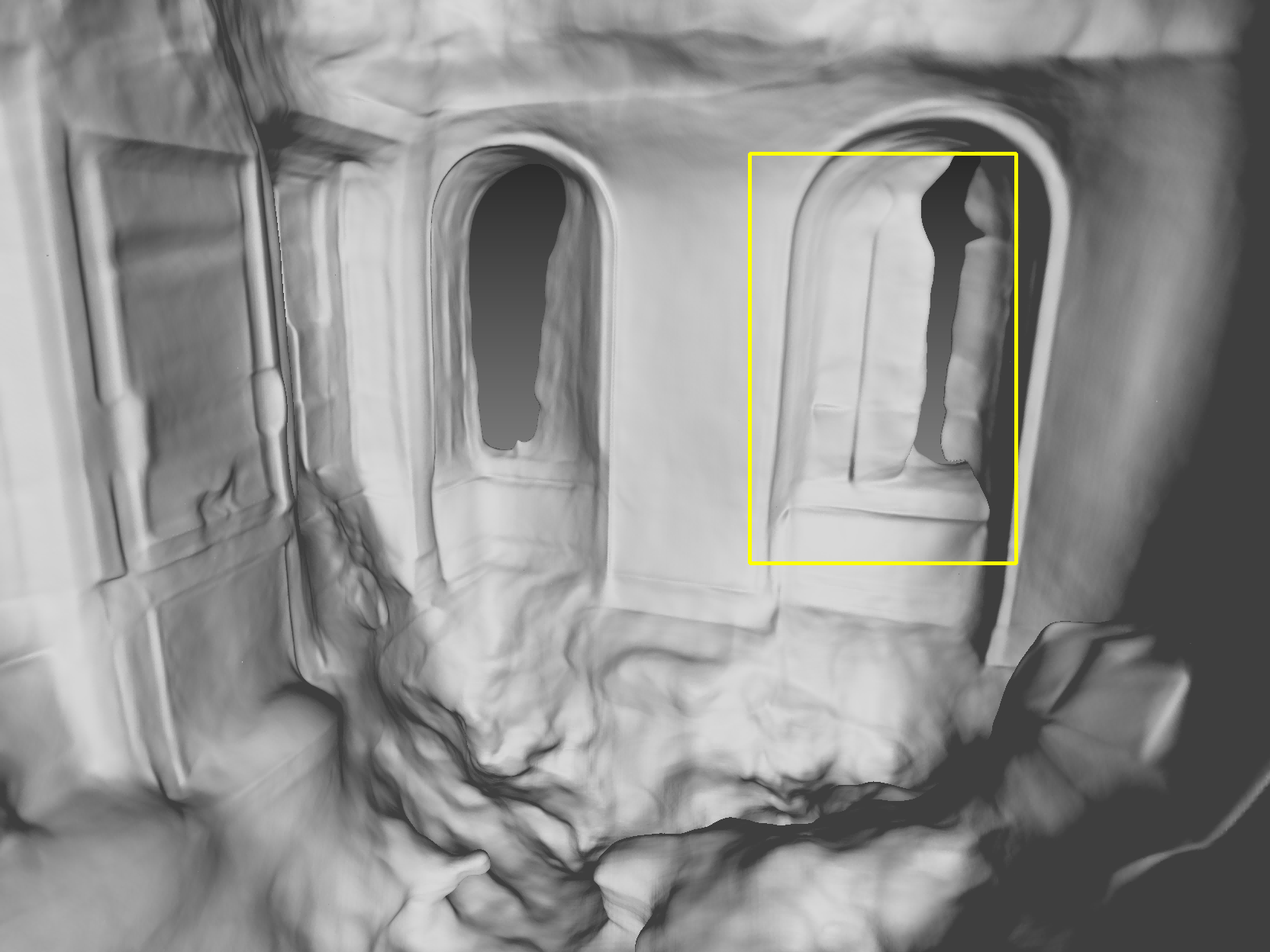
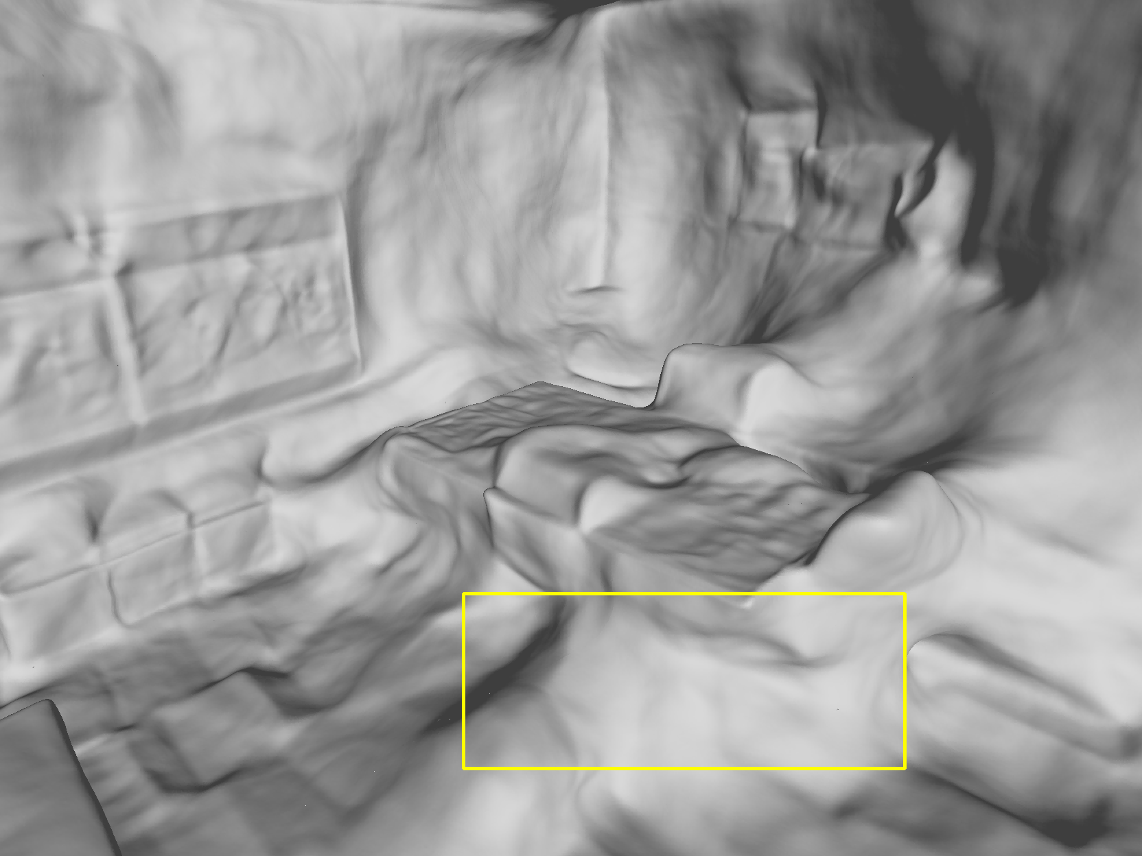
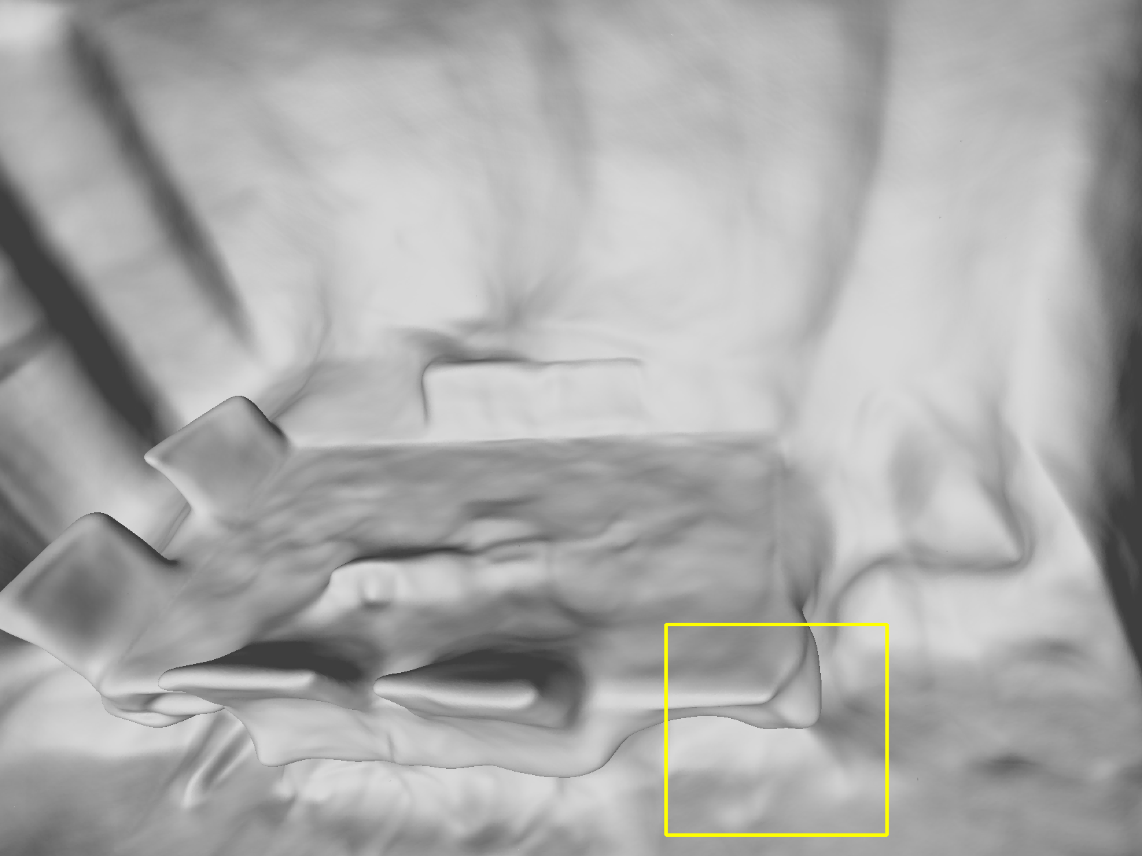
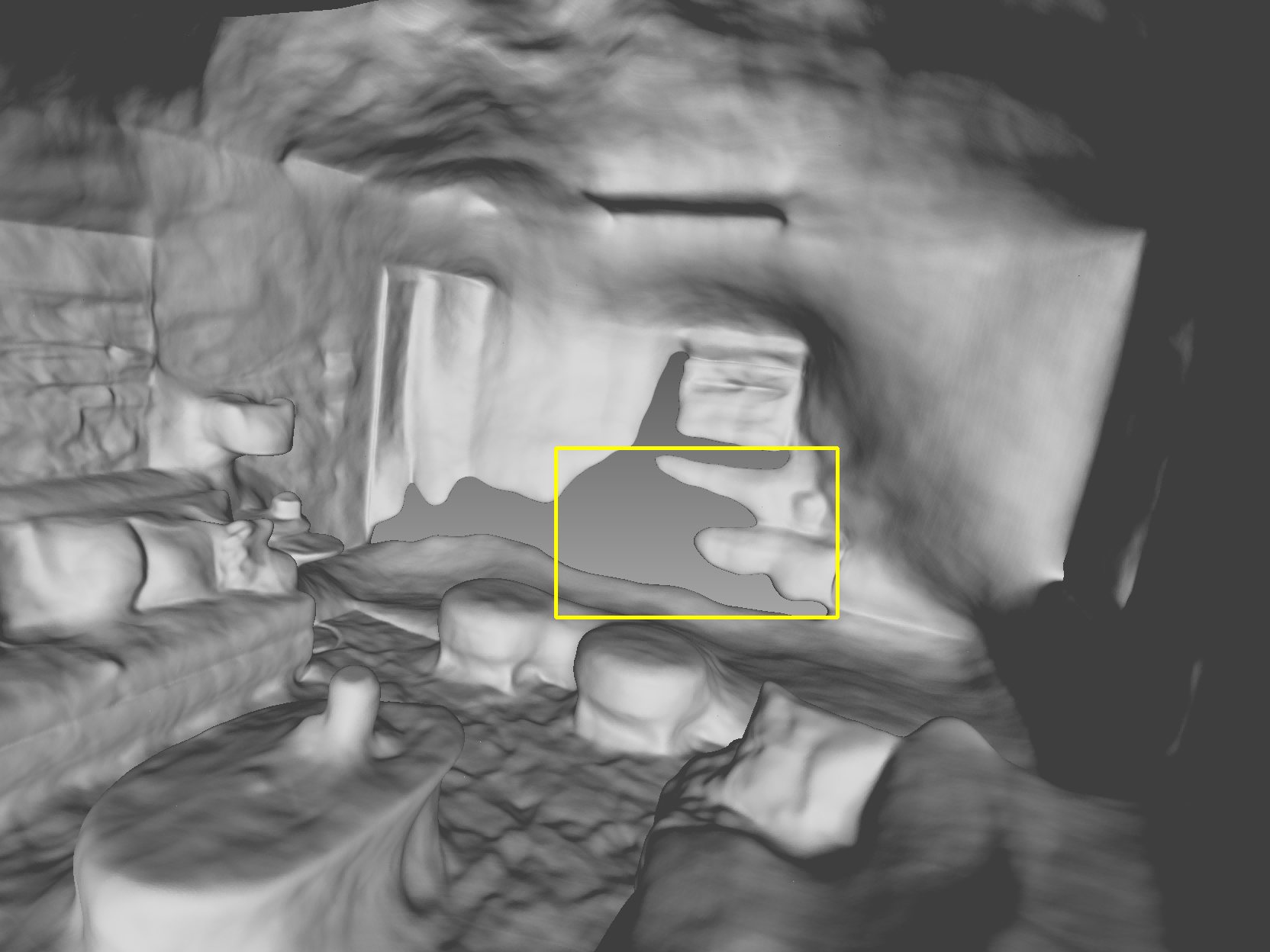
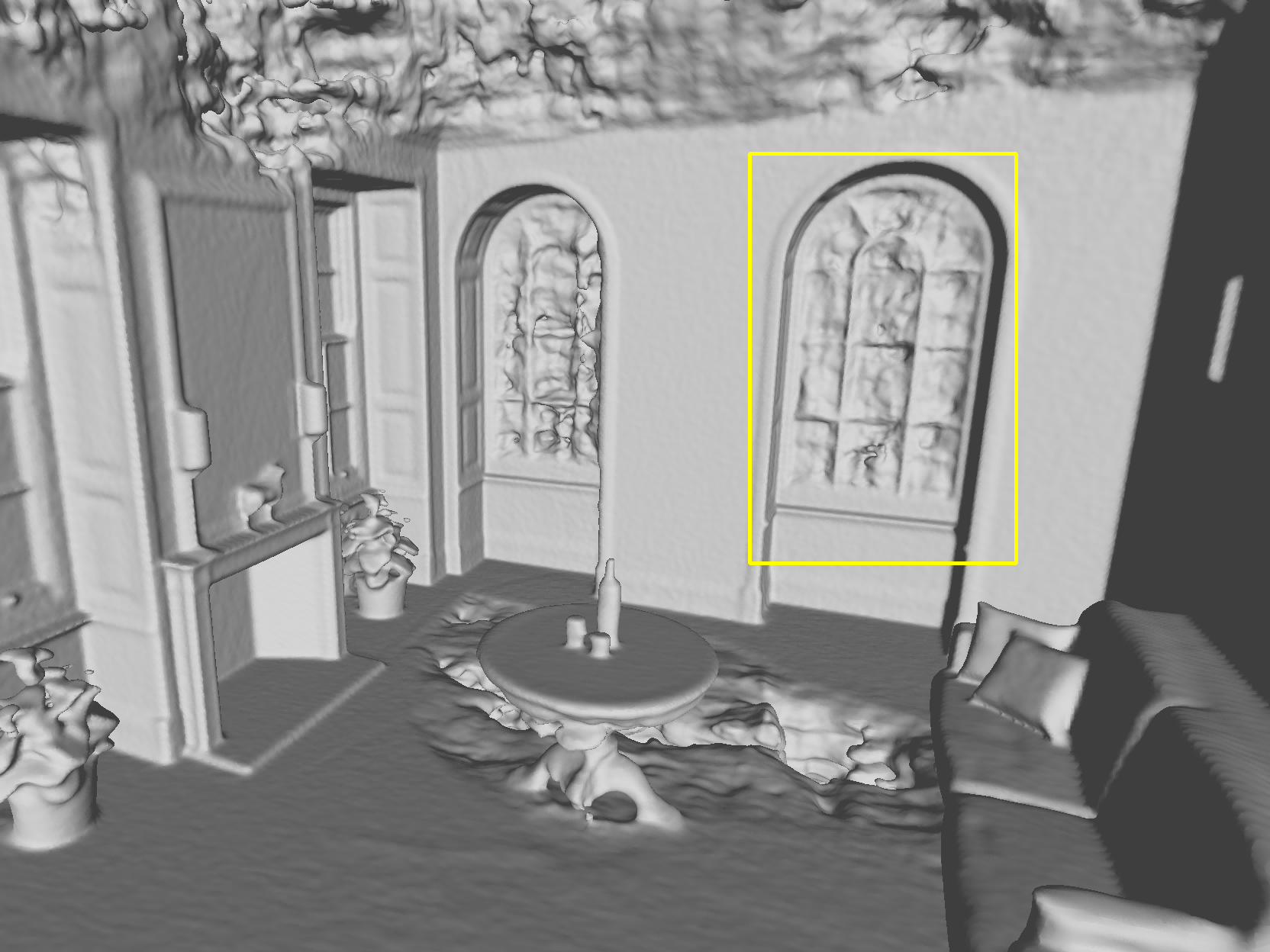
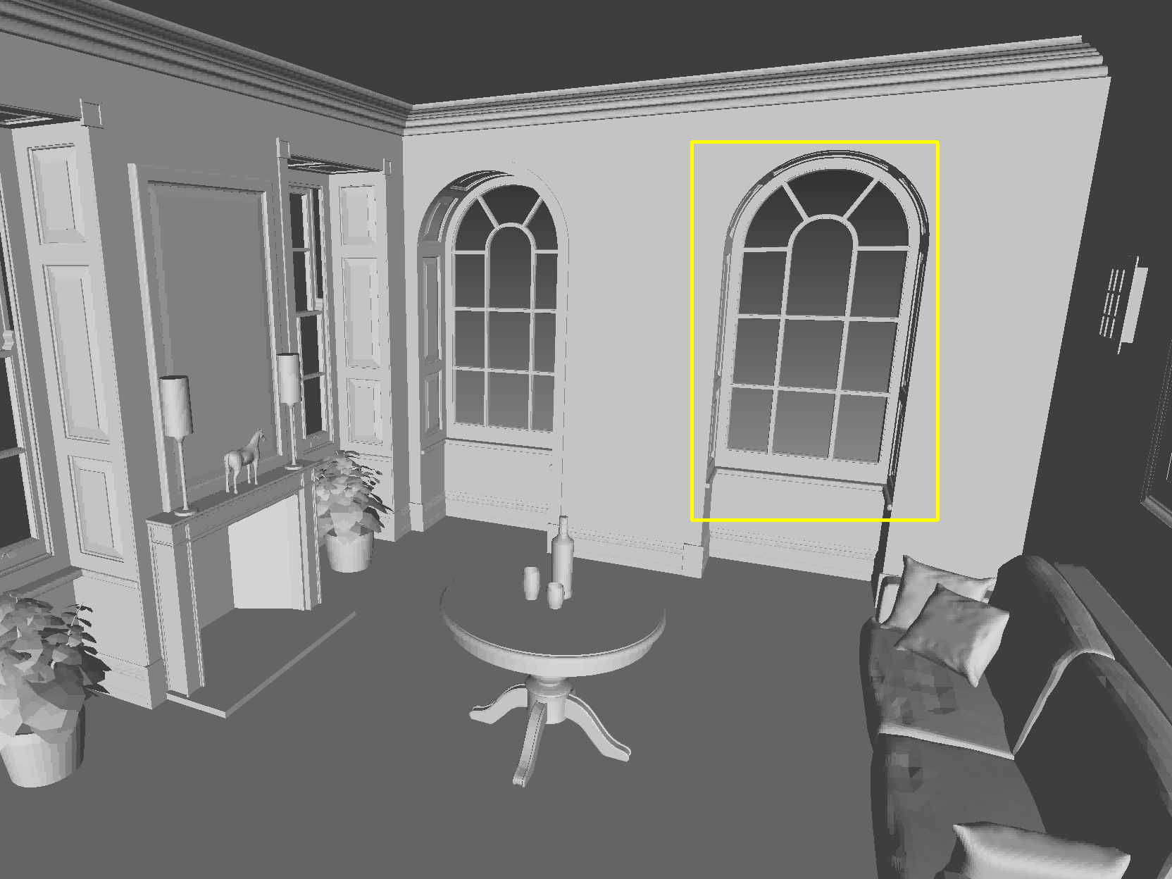
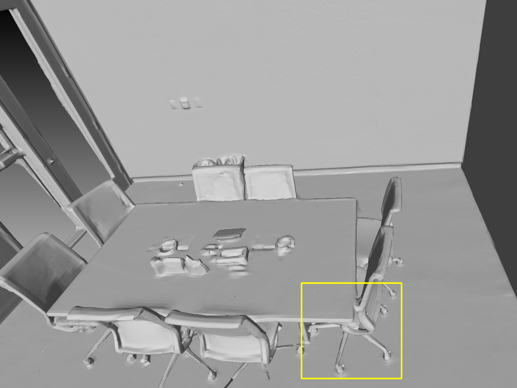
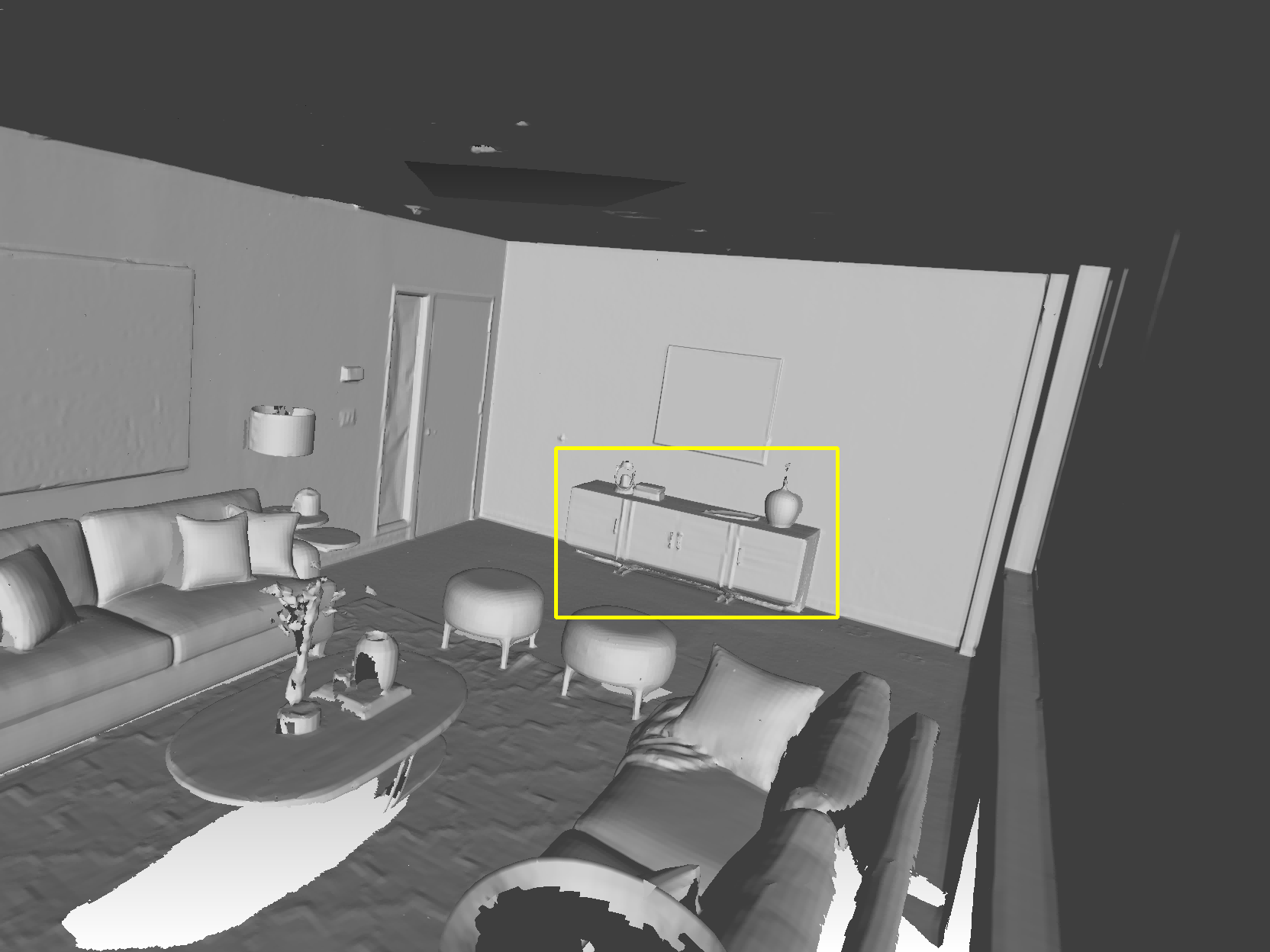
We compare the proposed method with BundleFusion, Neus, VolSDF, NeuralRGBD and Go-Surf in Scene Grey-white room, Office2, Office3, Room0 for geometry reconstruction, as shown in Fig. 7. Our method achieves the best visual result on all indoor scenes. It can be seen from Fig. 7 that our method has richer object details and smoother planes of indoor scenes. Specifically, Our method fills in the office chair legs completely and achieves a smoother result on the background walls and floors in the second and third columns. In the last column, our method is able to reconstruct the complete table compared to BundleFusion, Neus and NeuralRGBD, and refine the shape of the bottle compared to Go-Surf.
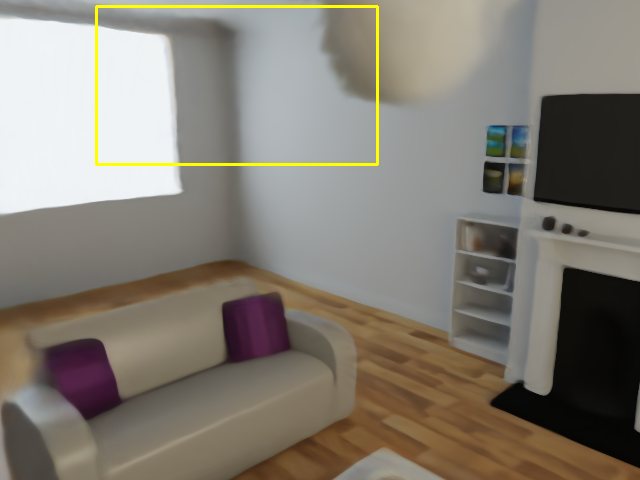
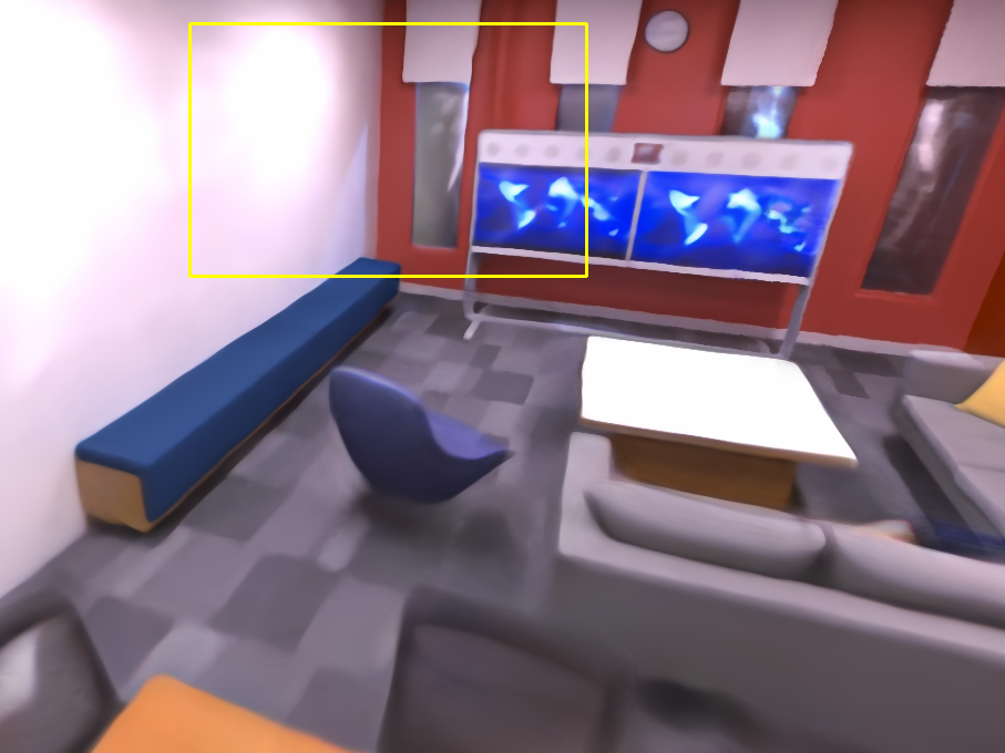
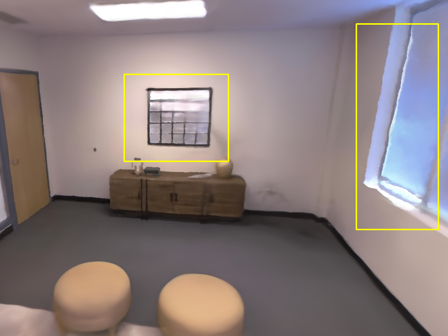
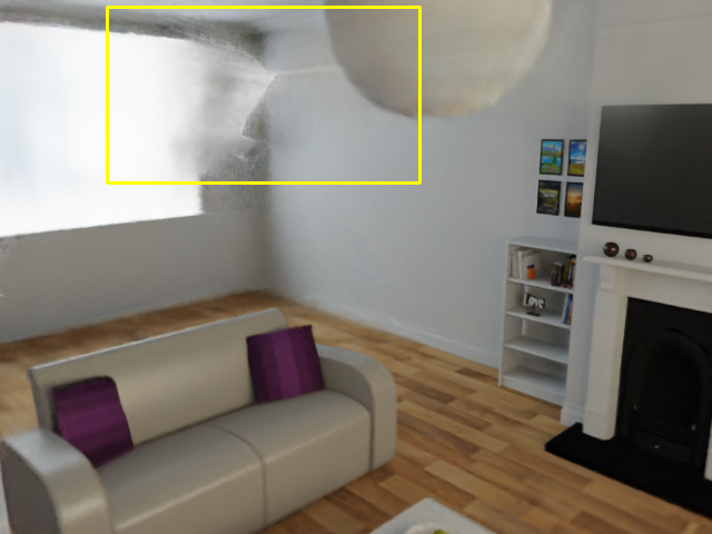
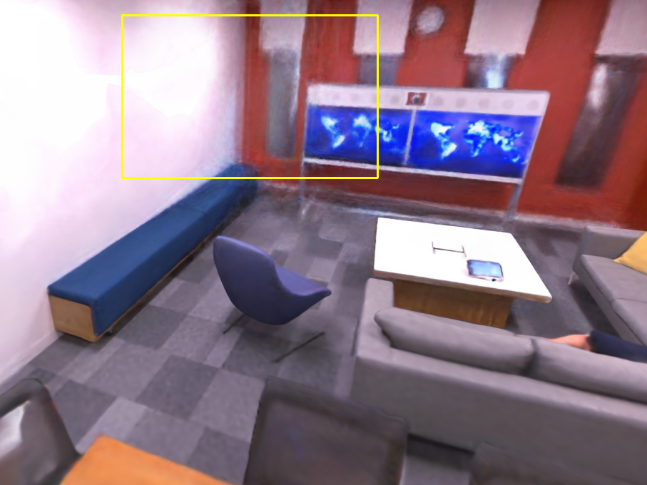
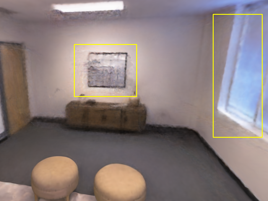
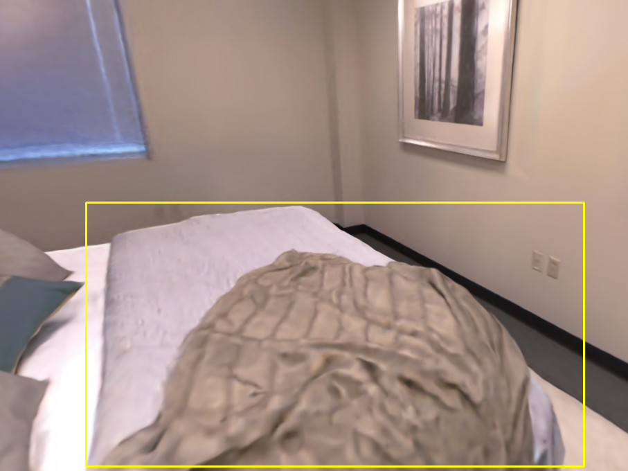
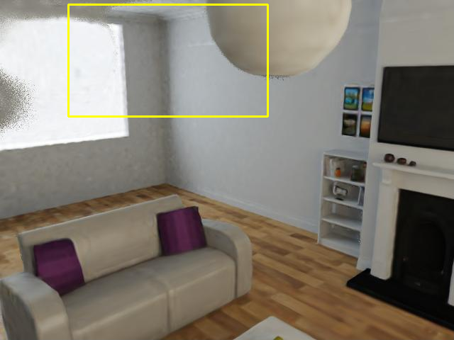
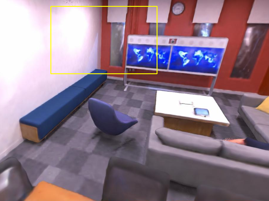
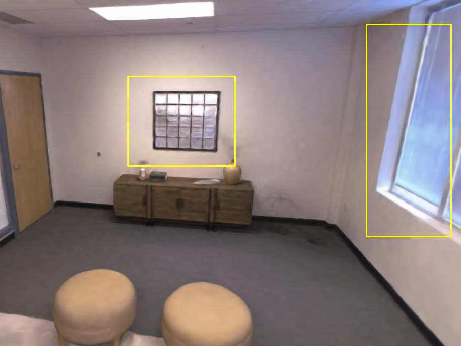
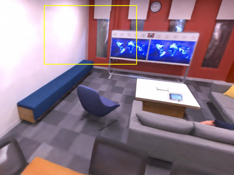
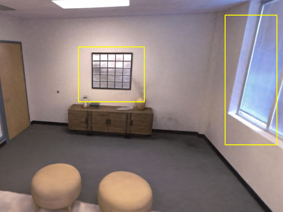
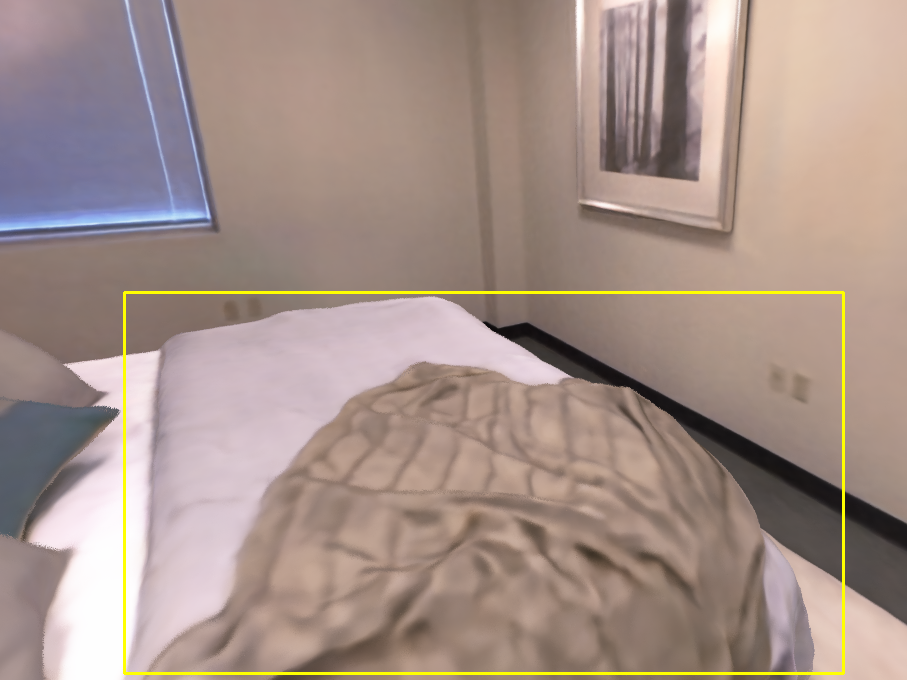
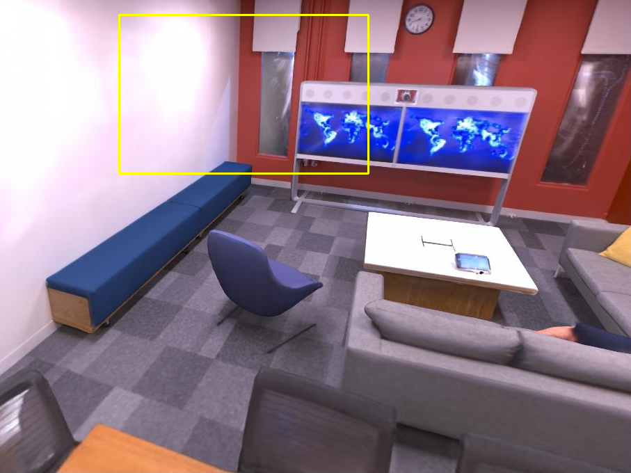
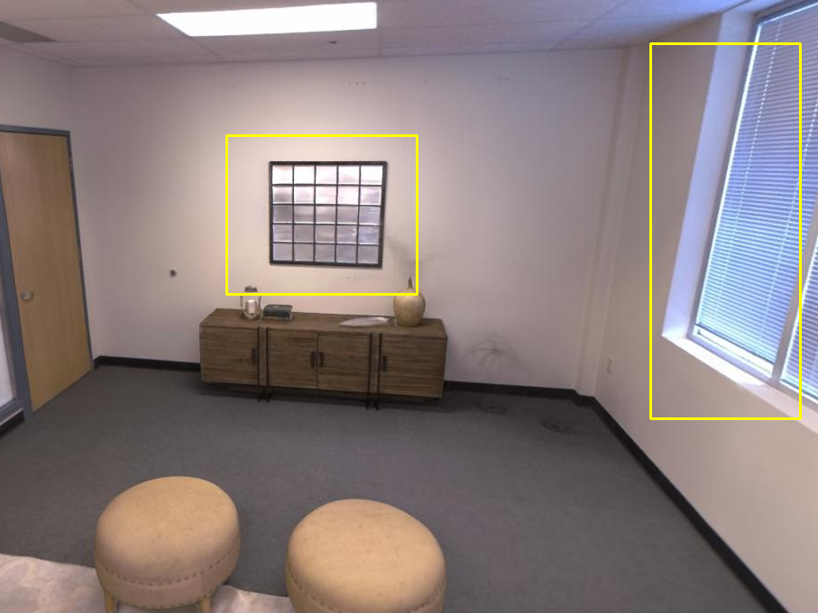
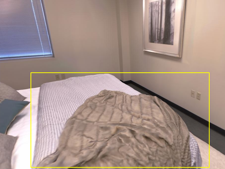
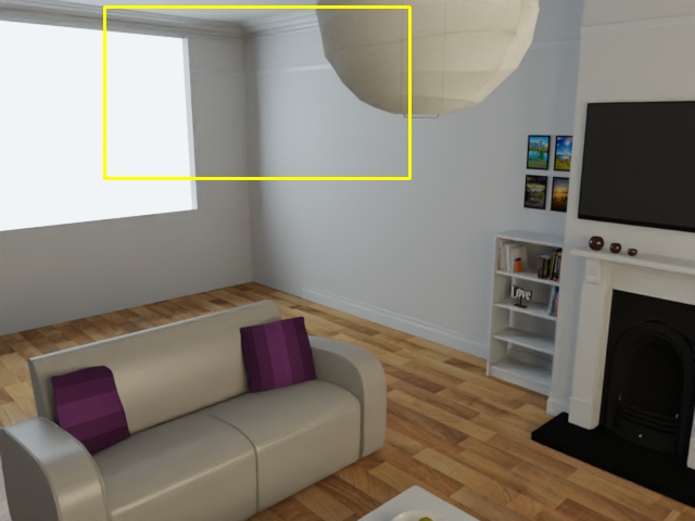
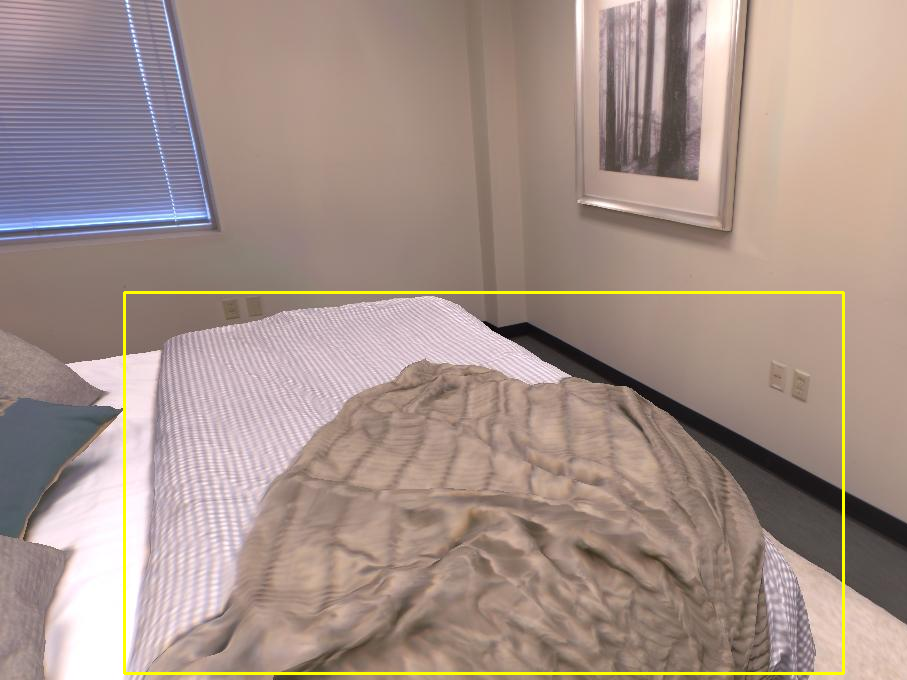
In addition, view synthesis performance on Whiteroom, Office3, Room0, and Room1 scenes of the Neus, InstantNGP, DVGO, Go-Surf and NeuralRGBD, are shown in Fig. 8. Our approach achieves the best image rendering results, in both the texture-less areas and rich texture areas. For instance, we accurately restore the appearance of texture-less regions such as ceiling corners in the first column and walls in the second and third columns. Additionally, we reproduce the details of complex texture regions, such as the shutter in the third column and the stripes of the quilt in the last column. Methods that focus on view rendering such as DVGO and InstantNGP suffer in texture-less or sparsely observed regions, as shown in the first and third columns of Fig. 8. Approaches focus on surface reconstruction, such as NeuralRGBD and Go-Surf, often struggle to get good view rendering results on areas of complex texture such as the windows in the third column and the quilt in the fourth column.
The detailed quantitative results on Replica dataset and NeuralRGBD dataset can be seen in Tab. 9 and in Tabs. 11 and 12, respectively. Our method obtains the SOTA rendering performance in all scenes and gives the highest performance in most of the scenes for geometry reconstruction.
| Scene | Scene size | Model size | Params. | Runtime |
|---|---|---|---|---|
| Breakfast room | MB | M | min | |
| Green room | MB | M | min | |
| Grey-white room | MB | M | min | |
| ICL living room | MB | M | min | |
| Complete kitchen | MB | M | min | |
| Kitchen | MB | M | min | |
| Morning apartment | MB | M | min | |
| Staircase | MB | M | min | |
| Thin Geometry | MB | M | min | |
| White room | MB | M | min | |
| Office0 | MB | M | min | |
| Office1 | MB | M | min | |
| Office2 | MB | M | min | |
| Office3 | MB | M | min | |
| Office4 | MB | M | min | |
| Room0 | MB | M | min | |
| Room1 | MB | M | min | |
| Room2 | MB | M | min |
8.2 More color decomposition results
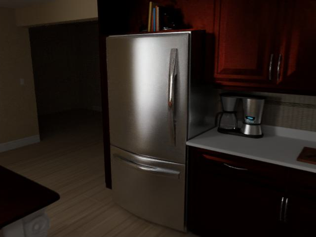
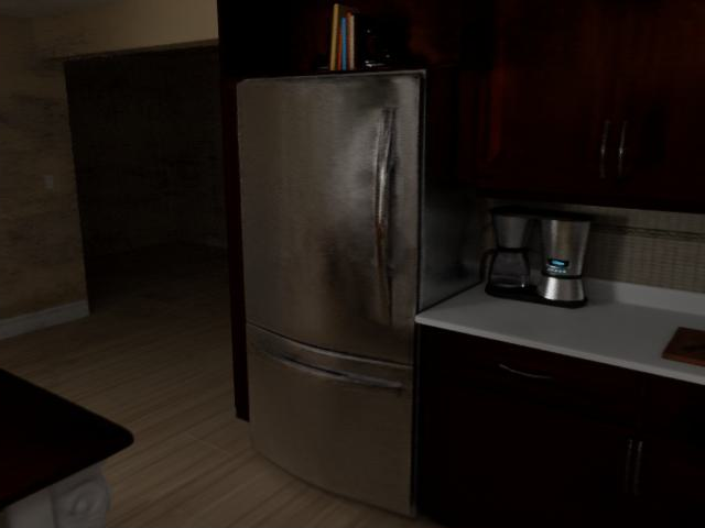
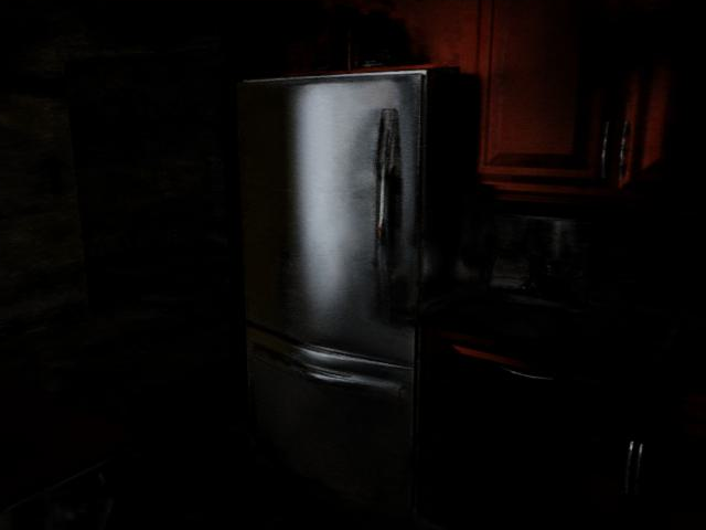
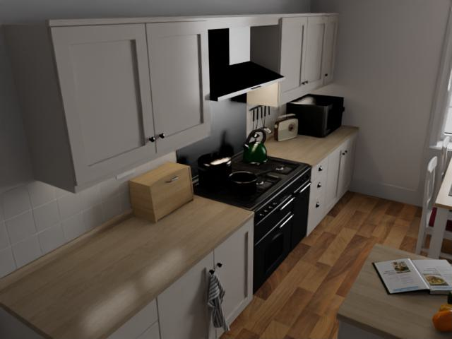
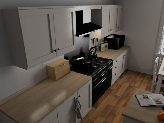
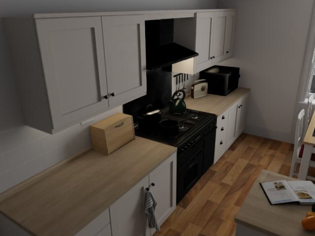
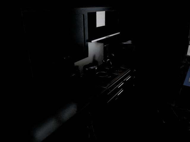
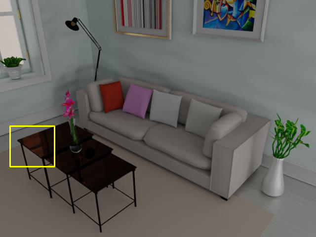
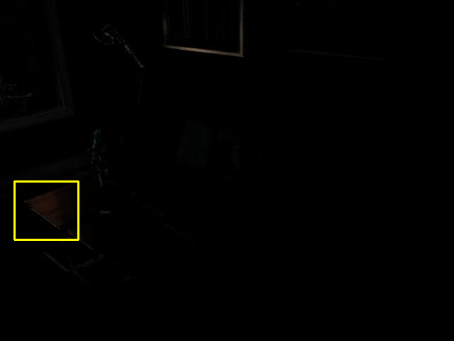
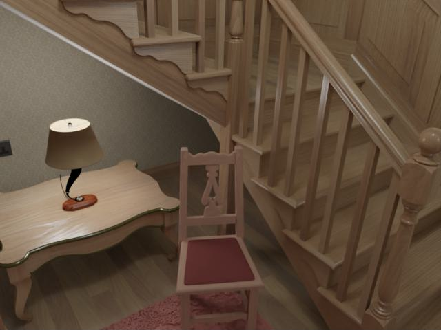
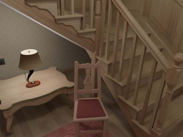
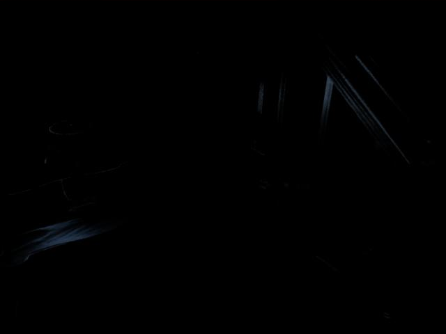
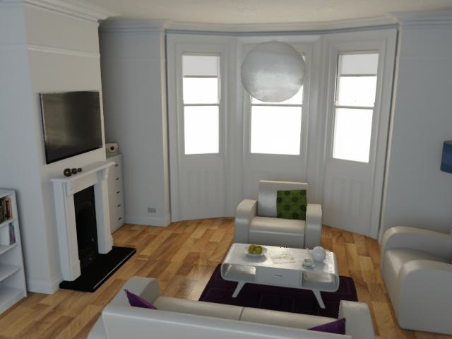
More color decomposition results are shown in Fig. 6. We can see that our method successfully decomposes the full color into view-independent color and view-dependent color such as the reflective table, the book and the TV.





BundleFusion
Neus
VolSDF
NeuralRGBD
Go-Surf

Ours
GT
Neus
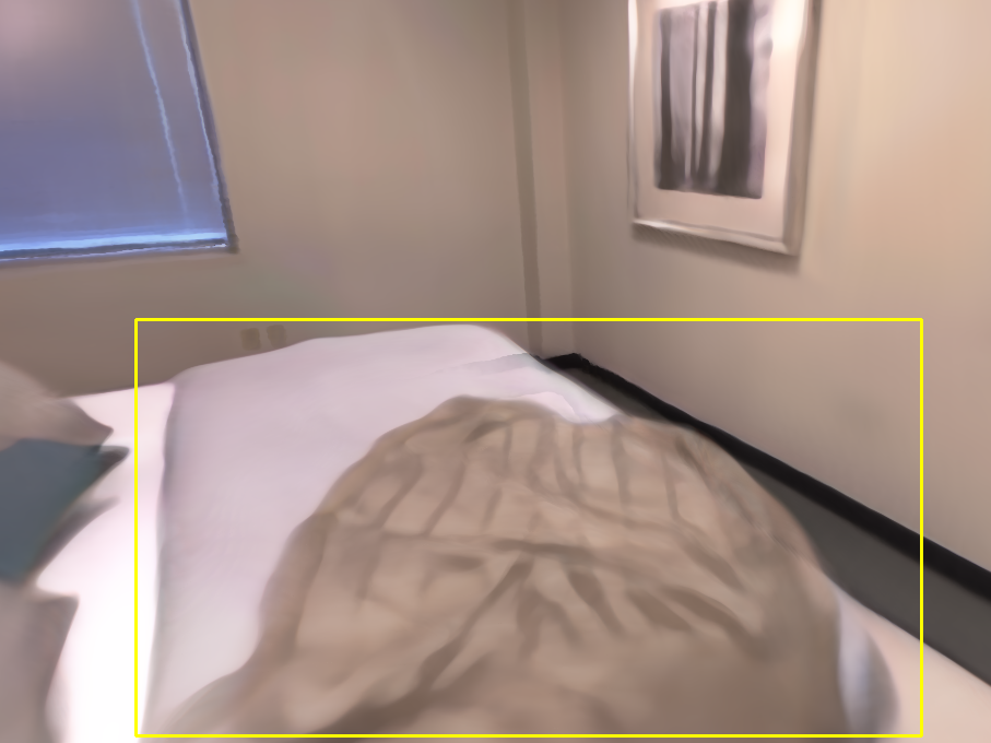

InstantNGP
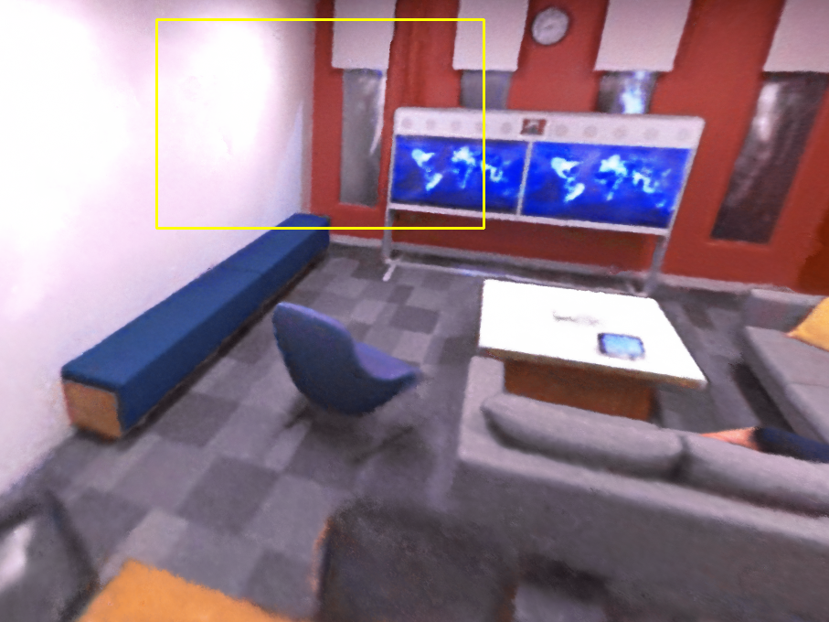
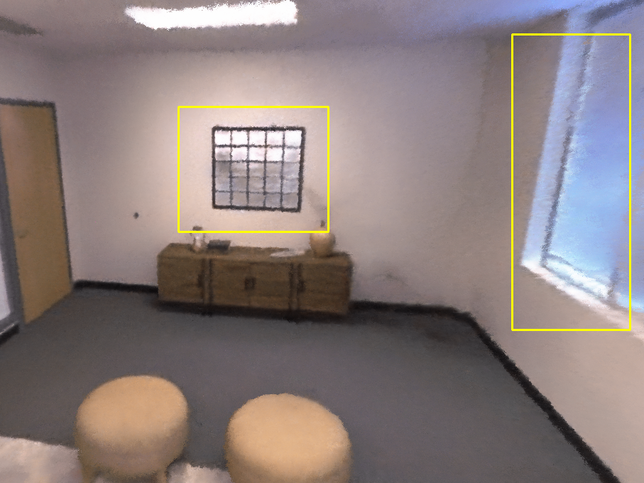
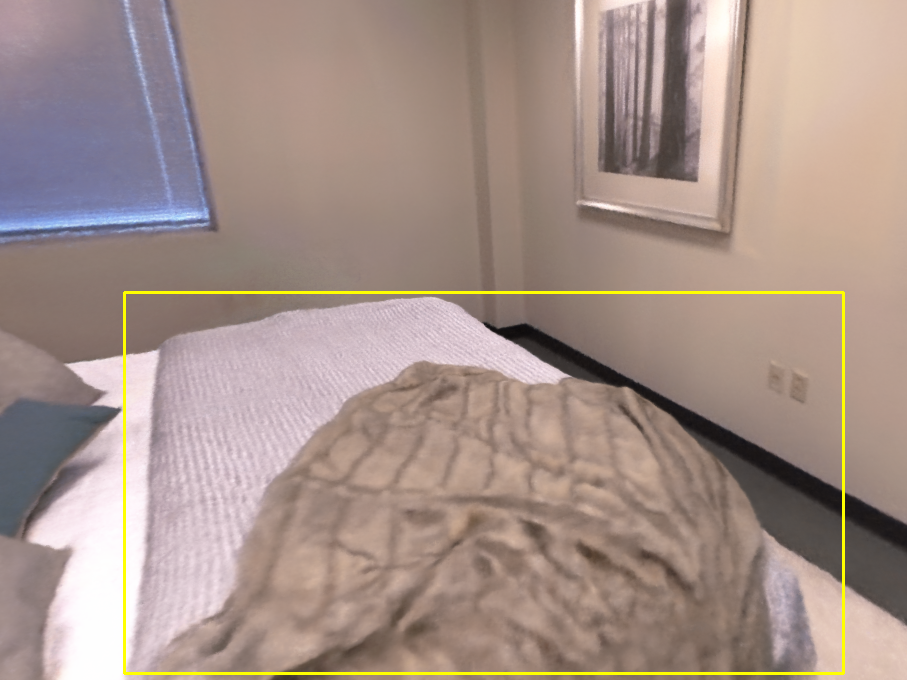
DVGO
Go-Surf


NeuralRGBD

Ours
GT


9 Runtime and Memory Requirements
There is a detailed breakdown of the runtime and memory usage in our experiments on all of the datasets, as shown in Tab. 10. It can be seen that our method could reach convergence in at most 1 hour on all scenes. Similar to previous methods that trade memory for time, Du-NeRF requires hundreds of MB to store the multi-resolution grid.
| Scene | Method | Acc | Com | C- | NC | F-score | PSNR | SSIM | LPIPS |
|---|---|---|---|---|---|---|---|---|---|
| Breakfast Room | BundleFusion | 0.0134 | 0.2000 | 0.1070 | 0.9170 | 0.8000 | - | - | - |
| Neus | 0.6270 | 0.7720 | 0.7000 | 0.6410 | 0.0100 | 27.2880 | 0.8230 | 0.1940 | |
| VolSDF | 0.0820 | 0.3360 | 0.2090 | 0.6880 | 0.2970 | 28.9610 | 0.8730 | 0.1570 | |
| NeuralRGBD | 0.0145 | 0.0148 | 0.0147 | 0.9650 | 0.9900 | 32.5340 | 0.9280 | 0.1090 | |
| GO-Surf | 0.0141 | 0.0150 | 0.0145 | 0.9630 | 0.9810 | 29.0600 | 0.8830 | 0.1650 | |
| InstantNGP | 0.2310 | 0.2970 | 0.2640 | 0.5670 | 0.2420 | 31.6560 | 0.8970 | 0.0853 | |
| DVGO | 0.5310 | 0.9010 | 0.7160 | 0.5100 | 0.0184 | 34.2720 | 0.9530 | 0.0640 | |
| Ours | 0.0141 | 0.0135 | 0.0138 | 0.9640 | 0.9860 | 38.2610 | 0.9830 | 0.0238 | |
| Complete Kitchen | BundleFusion | 0.0366 | 1.0780 | 0.5570 | 0.7470 | 0.4450 | - | - | - |
| Neus | 0.2950 | 1.5580 | 0.9270 | 0.5610 | 0.0641 | 26.3270 | 0.8410 | 0.2540 | |
| VolSDF | 0.3260 | 0.9100 | 0.6180 | 0.6800 | 0.1470 | 26.0160 | 0.8570 | 0.2400 | |
| NeuralRGBD | 0.0189 | 0.1100 | 0.0647 | 0.8960 | 0.8790 | 32.0310 | 0.9100 | 0.2020 | |
| GO-Surf | 0.0254 | 0.0295 | 0.0274 | 0.9395 | 0.8930 | 29.6040 | 0.8680 | 0.1760 | |
| InstantNGP | 0.1950 | 0.8730 | 0.5340 | 0.5740 | 0.2350 | 30.4066 | 0.8850 | 0.1470 | |
| DVGO | 0.2970 | 1.1580 | 0.7280 | 0.5610 | 0.1990 | 31.0570 | 0.9010 | 0.2180 | |
| Ours | 0.0222 | 0.0259 | 0.0240 | 0.9410 | 0.9010 | 34.5170 | 0.9520 | 0.0682 | |
| Green Room | BundleFusion | 0.0140 | 0.1965 | 0.1053 | 0.9090 | 0.8140 | - | - | - |
| Neus | 0.2130 | 0.3430 | 0.2780 | 0.7400 | 0.1130 | 29.4000 | 0.8930 | 0.1450 | |
| VolSDF | 0.1360 | 0.4320 | 0.2840 | 0.6490 | 0.2250 | 29.8840 | 0.9100 | 0.1380 | |
| NeuralRGBD | 0.0104 | 0.0140 | 0.0122 | 0.9340 | 0.9910 | 34.0800 | 0.9520 | 0.0770 | |
| GO-Surf | 0.0124 | 0.0156 | 0.0140 | 0.9275 | 0.9825 | 31.0520 | 0.9220 | 0.1170 | |
| InstantNGP | 0.2440 | 0.9710 | 0.6070 | 0.5370 | 0.1180 | 34.9470 | 0.9460 | 0.0364 | |
| DVGO | 0.2940 | 0.5190 | 0.4070 | 0.5640 | 0.2490 | 34.9800 | 0.9550 | 0.0760 | |
| Ours | 0.0122 | 0.0150 | 0.0136 | 0.9290 | 0.9850 | 38.5530 | 0.9780 | 0.0247 | |
| Grey White Room | BundleFusion | 0.0202 | 0.2743 | 0.1472 | 0.8230 | 0.7380 | - | - | - |
| Neus | 0.2620 | 0.4820 | 0.3720 | 0.6290 | 0.1160 | 28.7820 | 0.8630 | 0.1640 | |
| VolSDF | 0.1930 | 0.3360 | 0.2650 | 0.7070 | 0.2550 | 30.4400 | 0.8950 | 0.1480 | |
| NeuralRGBD | 0.0134 | 0.0151 | 0.0143 | 0.9310 | 0.9940 | 35.1630 | 0.9470 | 0.0900 | |
| GO-Surf | 0.0145 | 0.0167 | 0.0156 | 0.9255 | 0.9875 | 30.8900 | 0.9115 | 0.1490 | |
| InstantNGP | 0.1390 | 0.9380 | 0.5390 | 0.5010 | 0.1810 | 32.0200 | 0.8790 | 0.1270 | |
| DVGO | 0.2410 | 0.4430 | 0.3420 | 0.5640 | 0.2990 | 34.7160 | 0.9470 | 0.0930 | |
| Ours | 0.0140 | 0.0155 | 0.0147 | 0.9260 | 0.9900 | 37.7320 | 0.9700 | 0.0406 | |
| Icl Living Room | BundleFusion | 0.0104 | 0.2697 | 0.1400 | 0.9120 | 0.7720 | - | - | - |
| Neus | 0.3570 | 0.8040 | 0.5810 | 0.6270 | 0.1000 | 31.9550 | 0.9010 | 0.1090 | |
| VolSDF | 0.2520 | 0.8130 | 0.5330 | 0.6370 | 0.1450 | 30.6400 | 0.8980 | 0.1400 | |
| NeuralRGBD | 0.0089 | 0.0840 | 0.0462 | 0.9070 | 0.9010 | 34.3810 | 0.9300 | 0.1960 | |
| GO-Surf | 0.0101 | 0.0129 | 0.0115 | 0.9670 | 0.9910 | 31.7410 | 0.9080 | 0.2425 | |
| InstantNGP | 0.7180 | 1.8900 | 1.3000 | 0.5140 | 0.0100 | 27.1670 | 0.7650 | 0.2760 | |
| DVGO | 0.3000 | 0.8670 | 0.5830 | 0.5430 | 0.2130 | 33.9930 | 0.9330 | 0.2420 | |
| Ours | 0.0112 | 0.0140 | 0.0126 | 0.9690 | 0.9920 | 36.9860 | 0.9570 | 0.0638 |
| Scene | Method | Acc | Com | C- | NC | F-score | PSNR | SSIM | LPIPS |
|---|---|---|---|---|---|---|---|---|---|
| Kitchen | BundleFusion | 0.0170 | 0.5960 | 0.3065 | 0.8510 | 0.6390 | - | - | - |
| Neus | 0.4680 | 0.8490 | 0.6580 | 0.5740 | 0.0400 | 25.5880 | 0.8240 | 0.2340 | |
| VolSDF | 0.2130 | 0.3760 | 0.2950 | 0.7000 | 0.2810 | 25.7570 | 0.8520 | 0.2300 | |
| NeuralRGBD | 0.0198 | 0.1450 | 0.0824 | 0.9000 | 0.8630 | 31.6270 | 0.9170 | 0.1480 | |
| GO-Surf | 0.0204 | 0.0265 | 0.0235 | 0.9340 | 0.9430 | 27.8260 | 0.8735 | 0.2000 | |
| InstantNGP | 0.1620 | 0.6470 | 0.4050 | 0.5520 | 0.2360 | 29.3850 | 0.8650 | 0.1380 | |
| DVGO | 0.2690 | 0.5120 | 0.3900 | 0.5640 | 0.3340 | 30.5230 | 0.9360 | 0.1310 | |
| Ours | 0.0207 | 0.0266 | 0.0236 | 0.9330 | 0.9400 | 35.6100 | 0.9650 | 0.0458 | |
| Morning Apartment | BundleFusion | 0.0093 | 0.0153 | 0.0123 | 0.8880 | 0.9760 | - | - | - |
| Neus | 0.2130 | 0.2430 | 0.2280 | 0.6660 | 0.2180 | 27.5640 | 0.8370 | 0.2090 | |
| VolSDF | 0.0804 | 0.1450 | 0.1130 | 0.7300 | 0.3700 | 29.2440 | 0.8870 | 0.1660 | |
| NeuralRGBD | 0.0088 | 0.0117 | 0.0103 | 0.8920 | 0.9870 | 33.1350 | 0.9270 | 0.1080 | |
| GO-Surf | 0.0106 | 0.0145 | 0.0125 | 0.8840 | 0.9750 | 28.3880 | 0.8570 | 0.2245 | |
| InstantNGP | 0.4260 | 0.4920 | 0.4590 | 0.5030 | 0.1000 | 24.2740 | 0.6230 | 0.4640 | |
| DVGO | 0.1510 | 0.1760 | 0.1630 | 0.5480 | 0.5100 | 33.9590 | 0.9480 | 0.0740 | |
| Ours | 0.0099 | 0.0136 | 0.0118 | 0.8870 | 0.9780 | 36.6370 | 0.9660 | 0.0392 | |
| Staircase | BundleFusion | 0.0160 | 1.0020 | 0.5088 | 0.7960 | 0.4310 | - | - | - |
| Neus | 0.3800 | 0.8910 | 0.6360 | 0.6190 | 0.1140 | 29.4540 | 0.8430 | 0.2710 | |
| VolSDF | 0.1070 | 0.7340 | 0.4200 | 0.6720 | 0.2440 | 30.9470 | 0.8490 | 0.2570 | |
| NeuralRGBD | 0.0213 | 0.0441 | 0.0327 | 0.9420 | 0.9010 | 34.8610 | 0.9070 | 0.2210 | |
| GO-Surf | 0.0233 | 0.0285 | 0.0259 | 0.9490 | 0.8855 | 32.1520 | 0.8805 | 0.2560 | |
| InstantNGP | 0.2880 | 0.3240 | 0.3060 | 0.5820 | 0.3130 | 31.1140 | 0.8250 | 0.2320 | |
| DVGO | 0.2710 | 0.7460 | 0.5080 | 0.5750 | 0.2580 | 34.5150 | 0.9160 | 0.2200 | |
| Ours | 0.0221 | 0.0268 | 0.0244 | 0.9510 | 0.9280 | 36.7910 | 0.9550 | 0.0710 | |
| Thin Geometry | BundleFusion | 0.0227 | 0.0762 | 0.0495 | 0.8640 | 0.7160 | - | - | - |
| Neus | 0.1550 | 0.5760 | 0.3650 | 0.5380 | 0.0860 | 19.2300 | 0.7830 | 0.1760 | |
| VolSDF | 0.1140 | 0.3960 | 0.2550 | 0.5990 | 0.2710 | 24.7540 | 0.8900 | 0.1360 | |
| NeuralRGBD | 0.0093 | 0.0254 | 0.0173 | 0.9090 | 0.9420 | 18.9310 | 0.6600 | 0.5580 | |
| GO-Surf | 0.0107 | 0.0186 | 0.0146 | 0.9005 | 0.9440 | 25.8900 | 0.8820 | 0.1400 | |
| InstantNGP | 0.0821 | 0.4290 | 0.2560 | 0.6130 | 0.3070 | 32.4840 | 0.9330 | 0.0347 | |
| DVGO | 0.1040 | 0.0750 | 0.0900 | 0.5720 | 0.4750 | 35.1540 | 0.9680 | 0.0330 | |
| Ours | 0.0087 | 0.0122 | 0.0105 | 0.9070 | 0.9790 | 34.1260 | 0.9640 | 0.0286 | |
| Whiteroom | BundleFusion | 0.0184 | 0.8690 | 0.4440 | 0.8060 | 0.4700 | - | - | - |
| Neus | 0.2040 | 0.3930 | 0.2980 | 0.6820 | 0.1710 | 29.0620 | 0.8770 | 0.1610 | |
| VolSDF | 0.1240 | 0.3370 | 0.2300 | 0.7450 | 0.3870 | 30.5300 | 0.9050 | 0.1230 | |
| NeuralRGBD | 0.0202 | 0.0437 | 0.0320 | 0.9200 | 0.9098 | 33.1980 | 0.9330 | 0.1240 | |
| GO-Surf | 0.0225 | 0.0359 | 0.0292 | 0.9285 | 0.9070 | 29.2535 | 0.8985 | 0.1640 | |
| InstantNGP | 0.1560 | 0.4570 | 0.3060 | 0.6060 | 0.3370 | 31.7830 | 0.9090 | 0.0956 | |
| DVGO | 0.2230 | 0.5060 | 0.3650 | 0.5880 | 0.3130 | 33.1580 | 0.9400 | 0.0970 | |
| Ours | 0.0214 | 0.0340 | 0.0277 | 0.9270 | 0.9210 | 36.2280 | 0.9690 | 0.0409 |