Variance reduction via deflation with local coherence

Abstract

In large enough volumes, translation-averaging for quark-line connected diagrams reduces the variance inversely proportional to the volume. Stochastic estimators which implement translation averaging however introduce new sources of fluctuations, which in some cases can be relatively large. In this work, we explore whether inexact deflation subspaces can be used to improve the precision of the isovector vector correlators. We perform numerical experiments with $N_{\mathrm{f}}=2$ non-perturbatively $\mathrm{O}(a)$-improved Wilson fermions and measure the relative contribution from the deflation subspace to the central value and the corresponding variance.

1 Introduction

When translation averaging is used, the variance of observables with a small footprint is expected to decrease inversely proportional to the volume in a Monte Carlo simulation due to the mass gap of QCD [1]. While this idea certainly works out in the master-field regime [2], it has commonly been put into practice for moderate volumes, too. For quark-line connected correlation functions, such as the isovector vector correlator

$$\langle G(x,y_{0})\rangle_{\mathrm{g}} =\langle\tr\{W(x,y_{0},x)\}\rangle_{\mathrm{g}},\qquad W(x,y_{0},z)=-\tfrac{1}{3}\sum_{k}a^{3}\sum_{\bm{y}}\{S(x,y)\gamma_{k}S(y,z)\gamma_{k}\},$$ (1)

where $S(x,y)$ denotes the light-quark propagator and $\langle\cdot\rangle_{\mathrm{g}}$ denotes the average with respect to the effective action after integrating out the fermion fields, the variance shows a suppression proportional to the volume. This holds true even when integrating both vertices over the spatial volume $L^{3}$ in a box of linear size $L$. This can be understood from the expression for the variance for its translation-averaged counterpart $G_{\mathrm{vol}}(x_{0},y_{0})=\frac{a^{3}}{L^{3}}\sum_{\bm{x}}G(x,y_{0})$ which is

$$\sigma^{2}_{\mathrm{vol}}(x_{0}-y_{0}) =\frac{a^{3}}{L^{3}}\sum_{x^{\prime}}\delta_{x_{0}x_{0}^{\prime}}\Big{[}\langle G(x,y_{0})G(x^{\prime},y_{0})\rangle_{\mathrm{g}}-\langle G(x,y_{0})\rangle_{\mathrm{g}}\langle G(x^{\prime},y_{0})\rangle_{\mathrm{g}}\Big{]}$$ (2)

and noting the sum converges in infinite volume thanks to the extra suppression due to the quark propagators. Note also that the variance has no power-law divergences for $x_{0}\neq y_{0}$.

Implementing translation averaging is not completely straightforward without incurring a cost which also increases with the volume, for example if propagators would be explicitly computed from every lattice site. One possibility is to use a stochastic estimator for the translation average, such as the one-end trick [3, 4]

$$\mathcal{G}_{\mathrm{vol}}(x_{0},y_{0}) =\frac{1}{N_{\mathrm{src}}}\sum_{i=1}^{N_{\mathrm{src}}}\sum_{\alpha=1}^{4}\frac{a^{3}}{L^{3}}\sum_{\bm{x},z}\eta_{i}^{(\alpha)\dagger}(x)W(x,y_{0},z)\eta_{i}^{(\alpha)}(z)\delta_{x_{0}z_{0}}$$ (3)

where the dimensionless fields $\eta^{(\alpha)}_{i\beta c}(x)=\delta^{\alpha}_{\beta}\xi_{ic}(x)$ are defined in terms of i.i.d. random fields with zero mean and variance

$$\langle\xi_{ic}(x)\xi_{jd}^{*}(y)\rangle_{\xi} =\delta_{ij}\delta_{cd}\delta_{xy},$$ (4)

and we have chosen the spin-diagonal variant [5] which allows the unbiased estimation of each spin matrix element of $W$ with just $4N_{\mathrm{src}}$ inversions.

The introduction of new auxiliary fields leads to fluctuations, which, in the case of Gaussian-distributed fields, introduces an extra contribution to the variance [6]

$$\sigma^{2}_{\mathrm{stoch}}=\sigma^{2}_{\mathcal{G}}-\sigma^{2}_{\mathrm{vol}} =\frac{1}{N_{\mathrm{src}}}\sum_{\alpha,\beta=1}^{4}\sum_{a,b=1}^{3}\sum_{\bm{x},z}\delta_{x_{0}z_{0}}\langle W_{\alpha a,\alpha b}(x,y_{0},z)W_{b\beta,a\beta}(z,y_{0},x)\rangle_{\mathrm{g}}.$$ (5)

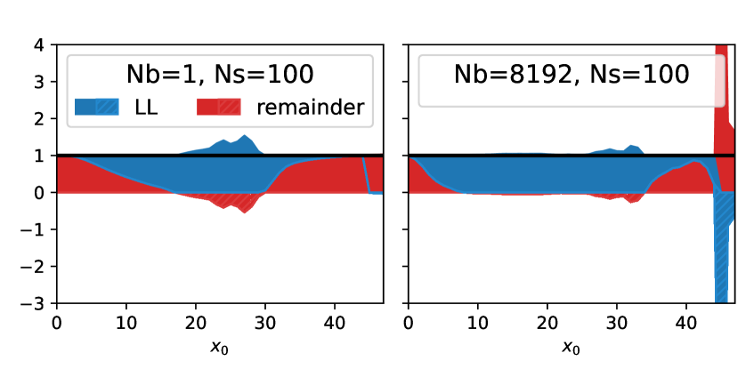
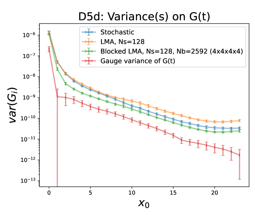
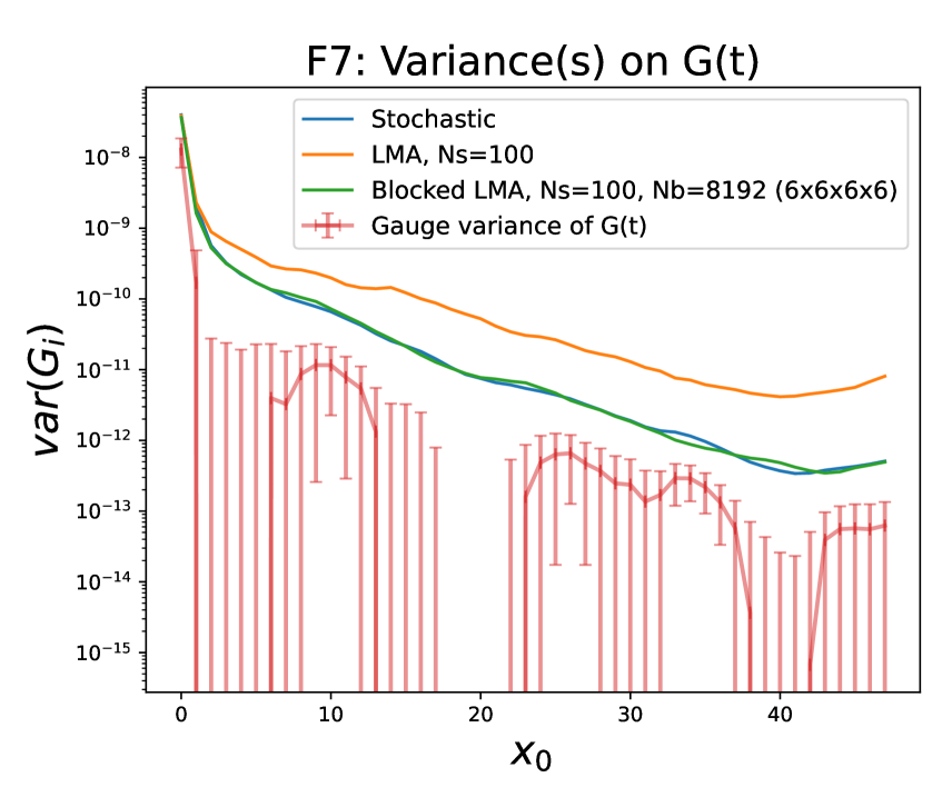
Although its volume-scaling is the same as the exact average in Eq. (2), it has different matrix elements which can be relatively large compared to $\sigma^{2}_{\mathrm{vol}}$, potentially spoiling the variance-reduction from translation averaging. This is illustrated in Fig. 4 where we depict estimators for the variances $\sigma^{2}_{\mathrm{vol}}$ (red) and $\sigma^{2}_{\mathrm{stoch}}\approx\sigma^{2}_{\mathcal{G}}$ (blue) for the isovector vector correlator showing the large hierarchy between them even when $N_{\mathrm{src}}$ is large. In the following we investigate improved estimators based on deflation techniques.

2 Variance reduction via deflation

Natural decompositions of traces such as Eq. (1) can be constructed starting from a decomposition of the quark propagator defined in terms of a set of $N$ linear independent fields $\phi_{1}(x),\ldots,\phi_{N}(x)$

$$S(x,y) =\sum_{k,l=1}^{N}\phi_{k}(x)(A^{-1})_{kl}\phi_{l}^{\dagger}(y)+P_{\mathrm{R}}S(x,y),$$ (6)

where the first term represents the propagator within the subspace of fields, and the matrix elements of the so-called little Dirac operator $A$ are defined explicitly in terms of the Dirac operator $D$

$$A_{kl} =(\phi_{k},D\phi_{l}).$$ (7)

Such operators arise when considering the Schur complement of the propagator in the subspace. The remainder may be written in terms of the projected propagator, namely

$$P_{\mathrm{R}}S(x,y) =S(x,y)-\sum_{k,l=1}^{N}\phi_{k}(x)(A^{-1})_{kl}\phi_{l}^{\dagger}(y).$$ (8)

Inserting the representation Eq. (6) into Eq. (1), the trace may be decomposed into terms involving only the little propagator $A^{-1}$ and a remainder. If the fields are chosen to be exact (left) singular vectors of the Dirac operator, the former contribution can be computed exactly with translation averaging. When the remainder is computed stochastically, the extra contribution to the variance has the same form as Eq. (5) with at least two insertions of $P_{\mathrm{R}}$. The efficiency of the deflation for our purposes is thus measured by the reduction in the variance. In practice, we note that the dimension of the little propagator is too large to compute and store directly, and thus its contributions may also need to be estimated stochastically. Nevertheless, here we will assume it is cheap enough that the extra contribution to the variance can be suppressed by a sufficiently large number of samples $N_{\mathrm{src}}$.

Such low-mode averaging and its variants are common variance-reduction strategies in lattice QCD and have been known for a long time [7, 8]. However, given that the spectral density increases with the volume, the cost of achieving a constant efficiency with the volume scales with its square. Volume scaling e.g. achieved in inexact deflation [9] and multigrid solvers [10] profits from the local coherence of the low modes of the Dirac operator. That is, the low modes projected to local domains can be represented by a small basis of fields to a high degree of precision. In this way, only a small number of exact modes are required to span a much larger deflation subspace and the volume-scaling problem is circumvented, as outlined in the following section.

2.1 Domain-decomposed subspaces

A domain-decomposed subspace of dimension $N$ may be constructed from a much smaller set of $N_{\mathrm{s}}$ input fields $\psi_{1}(x),\ldots,\psi_{N_{\mathrm{s}}}(x)$ in the following way. By decomposing the lattice into a set of $N_{\mathrm{b}}$ non-overlapping blocks labelled by $\Lambda$, the input fields are projected to the blocks

$$\psi_{k}^{\Lambda}(x) =\begin{cases}\psi_{k}(x)&\textrm{if $x\in\Lambda$},\\ 0&\textrm{otherwise}\end{cases}$$ (9)

and re-orthogonalized afterwards. After relabelling the $N=N_{\mathrm{b}}N_{\mathrm{s}}$ fields one implements the deflation exactly as described in the previous subsection. In contrast to the input fields used in the preconditioning of the Dirac equation [9] which may be fairly rough approximations of the low modes, initialized for example through a few inverse iterations, we have in mind to take the input fields as exact (left) singular vectors of the lattice Dirac operator. Such domain decompositions have been utilized as a compression algorithm [11] as well as variance reduction similar to what we investigate here [12].

3 Numerical experiments

Name	$T\times L^{3}$	Pion mass	$a$ [fm]	$\#$ configs
D5d	$48\times 24^{3}$	$439$ MeV	$0.0658(10)$	100
F7	$96\times 48^{3}$	$268$ MeV	$0.0658(10)$	100

Table 1: Ensembles of $N_{\mathrm{f}}=2$ non-perturbatively $\mathrm{O}(a)$-improved Wilson fermions used in this work.

In this section, we present some numerical investigations of domain-decomposed deflation subspaces using $N_{\mathrm{f}}=2$ non-perturbatively $\mathrm{O}(a)$-improved Wilson fermions generated by the Coordinated Lattice Simulations (CLS) effort [13]. We study two ensembles of representative gauge field configurations separated widely in Monte Carlo time and whose parameters are listed in Tab 1. A small number of input fields $N_{\mathrm{s}}\sim 10-100$ were created on each configuration using the PRIMME library [14] to a relative precision of $10^{-12}$. The stochastic sources $\eta$ were spin-diagonal with $\mathbb{Z}_{2}\times\mathbb{Z}_{2}$ noise. We report results only for the case of the isovector vector current correlator as defined in Eq. (1).

3.1 Efficiency of domain-decomposed subspaces

In order to illustrate one sense in which the enlarged space of fields represents the true low-mode subspace well, one can examine the deficits $\epsilon_{i}$ of the exact low modes $\chi_{i}$ which are not contained in the domain-decomposed subspace

$$\epsilon_{i}=\norm{\chi_{i}-\textstyle\sum_{k=1}^{N}\phi_{k}(\phi_{k},\chi_{i})}/\norm{\chi_{i}}$$ (10)

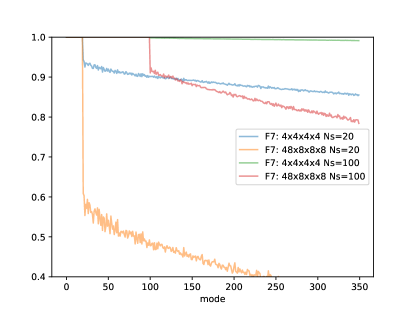
In Fig. 1, we display the deficits of the first few hundred exact low modes on the F7 ensemble for various subspaces created from two choices of number of input fields $N_{\mathrm{s}}=20,100$ and two configurations of the domain sizes namely $4^{4}$ and $48\times 8^{3}$ in lattice units, which correspond to domains in the spatial sizes of around $0.25$ and $0.5\,\mathrm{fm}$ respectively. The subspace size is thus increased by a factor $41472$ or $432$ in each case by the domain decomposition. As expected, the deficits are reduced by decreasing the domain size and by increasing the number of input modes. However, as explained previously, the precise measure of the efficiency for our purpose is whether the stochastic variance of the remainder terms is reduced compared to the undeflated version, which we investigate in the following subsection.

Figure 1: Local coherence of low modes. The deviation of the deficits Eq. (10) from unity $1-\epsilon_{i}$ versus the mode number. The first $N_{\mathrm{s}}$ modes in each case are exactly contained in the enlarged subspace by construction and have zero deficit. The deficits are reduced by decreasing the domain size or by increasing $N_{\mathrm{s}}$ the number of input modes.

3.2 Efficiency of variance reduction

In this section we test the efficiency of the deflation in reducing the variance on the individual contributions to the trace in Eq. (1) for various domain decompositions. Using the deflation subspace as defined above, we make the decomposition of the stochastic estimator of Eq. (3)

$$\mathcal{G}_{\mathrm{vol}} =\mathcal{G}^{\mathrm{lttl}}_{\mathrm{vol}}+\mathcal{G}^{\mathrm{rem}}_{\mathrm{vol}}$$ (11)

where the two estimators are defined as follows. The first contains only the little propagators

$$\mathcal{G}^{\mathrm{lttl}}_{\mathrm{vol}}(x_{0},y_{0}) =\frac{1}{N_{\mathrm{src}}}\sum_{i=1}^{N_{\mathrm{src}}}\sum_{\alpha=1}^{4}\frac{a^{6}}{L^{3}}\sum_{\bm{x},\bm{y},z}\delta_{x_{0}z_{0}}\Big{[}$$

$$\qquad\sum_{klmn=1}^{N}\eta_{i}^{(\alpha)\dagger}(x)\phi_{k}(x)(A^{-1})_{kl}\phi_{l}^{\dagger}(y)\gamma_{k}\phi_{m}(y)(A^{-1})_{mn}\phi^{\dagger}_{n}(z)\gamma_{k}\eta_{i}^{(\alpha)}(z)\Big{]}$$ (12)

while the remainder contains a mixed term and a term arising only from the projected propagator

$$\mathcal{G}^{\mathrm{rem}}_{\mathrm{vol}}(x_{0},y_{0}) =\frac{1}{N_{\mathrm{src}}}\sum_{i=1}^{N_{\mathrm{src}}}\sum_{\alpha=1}^{4}\frac{a^{6}}{L^{3}}\sum_{\bm{x},\bm{y},z}\delta_{x_{0}z_{0}}\Big{[}2\sum_{kl=1}^{N}\eta_{i}^{(\alpha)\dagger}(x)\phi_{k}(x)(A^{-1})_{kl}\phi_{l}^{\dagger}(y)\gamma_{k}P_{\mathrm{R}}S(y,z)\gamma_{k}\eta_{i}^{(\alpha)}(z)$$

$$\qquad\qquad\qquad\qquad+\eta_{i}^{(\alpha)\dagger}(x)P_{\mathrm{R}}S(x,y)\gamma_{k}P_{\mathrm{R}}S(y,z)\gamma_{k}\eta_{i}^{(\alpha)}(z)\Big{]}.$$ (13)

As explained earlier, we assume that in practice the little propagator is cheap enough so that $N_{\mathrm{src}}$ can be chosen very large for that term. We note, however, that the one-end trick estimator is recovered if $N_{\mathrm{src}}$ is chosen to be the same for both terms with the same noise fields. It is therefore interesting to examine each term in turn with a fixed number of $N_{\mathrm{src}}$, keeping in mind that the variance can be effectively eliminated on the little term at no cost.

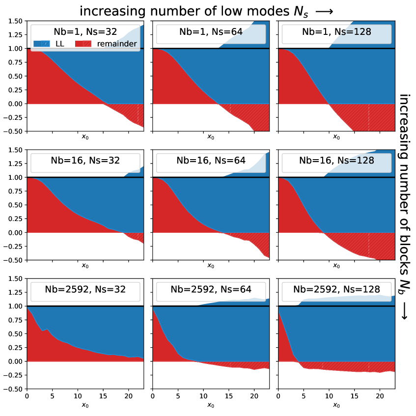
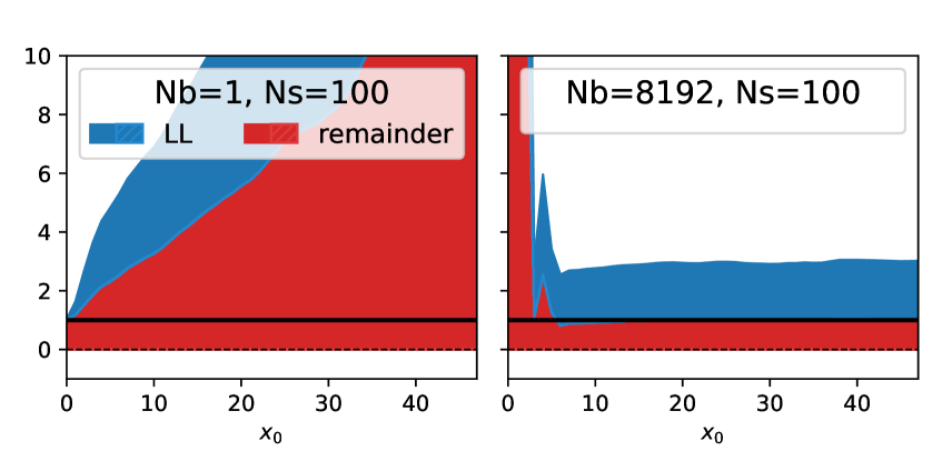
In Figs. 2 and 3 we show the relative contribution of the two terms to both the central value and the variance as a function of $x_{0}-y_{0}$. In the left panels, the relative contribution to the central value of the little term (blue) and the remainder term (red) is shown normalized by the sum. Each panel represents a different choice of parameters, with the number of blocks $N_{\mathrm{b}}$ increasing from left to right, and the number of input fields $N_{\mathrm{s}}$ increasing from top to bottom. Note that the remainder term, representing the contribution from the high modes dominates at small separations but even becomes negative at large separations.

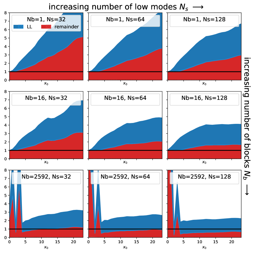
In the right panel, we show the variances of the little term (blue) and the remainder (red), normalized by the variance of the sum. The striking feature is the large size of the variance from the remainder term even at the largest separations. Except for the largest deflation subspace sizes (bottom right), this illustrates that the variance on the one-end trick estimator is smaller than the individual contributions, which demonstrates the high degree of covariance between the two pieces. That is, the stochastic variance on the remainder is not guaranteed to be smaller than the original estimator. Even if the variance due to the little propagator is eliminated by increasing the number of samples, the variance on the remainder (red) is larger than the original estimator (black line) except for the smallest domain size of $4^{4}$ for the D5d ensemble (Fig. 2 right, bottom row).

Figure 2: Left: Relative contributions to the value of the correlator Eq. (1), on D5d lattice using different number of low modes $N_{\mathrm{s}}$ and different number of blocks $N_{\mathrm{b}}$ increasing left to right and top to bottom respectively. Right: The variance of the little contribution (blue) and remainder (red) normalized by the variance of the sum. The block sizes ($T\times L^{3}$) are; 1st row: no blocking (corresponding to traditional LMA), 2nd row: $24\times 12\times 12\times 12$, 3rd row: $4\times 4\times 4\times 4$.

Figure 3: Same as Fig. 2 for the F7 ensemble. The block sizes ($T\times L^{3}$) are; left: no blocking (LMA) right: $6\times 6\times 6\times 6$.

Figure 4: Comparison of variances of the one-end trick (blue), deflated (yellow) and deflation with domain-decomposed subspace estimators (green). An estimator for the variance of the exact translation average Eq. (2) is shown in red. D5d (left) and F7 (right) with $N_{\mathrm{s}}=128,100$ low modes and $N_{\mathrm{src}}=32,96$ stochastic spin-diagonal sources, respectively.

4 Conclusions

In this work we presented a preliminary investigation into variance reduction using deflation with domain-decomposed subspaces for the isovector vector correlator with $N_{\mathrm{f}}=2$ non-perturbatively $\mathrm{O}(a)$-improved Wilson fermions. Such a domain decomposition exploits the local coherence of the low quark modes of the Dirac operator that almost eliminates the volume-squared problem of generating such subspaces. Variance reduction methods are required for the vector channel due to the large contribution to the variance from the noise fields, as can be seen in Fig. 4 where we computed an estimator for the variance of the translation-averaged observable Eq. (2).

For the few subspace configurations that we investigated, we observed that in many cases deflating the stochastic estimator may actually increase the variance. In Fig. 4 (left) for the ensemble with larger quark-mass, we see a moderate reduction in the variance with the best parameter choice (green) over the one-end trick (blue). For the smaller quark mass ensemble (right), the variance is at best identical to the case of the one-end trick. We note that in traditional low-mode averaging (yellow), the variance is actually increased with respect to the one-end trick estimator (blue) with these parameter choices and for this observable. Therefore, in order to be safe, a careful analysis of the variances can be is important to gauge the efficiency of deflation. Clearly, there are many possible choices to further improve the estimation of the remainder term (particularly the cross term) which was computed in a simple way in this work, which is ongoing, as well as work towards a more efficient implementation. A more thorough theoretical analysis of low-mode deflation on the variances would be beneficial to better motivate the definition of the subspace.

References

- [1] Martin Lüscher “Stochastic locality and master-field simulations of very large lattices” In EPJ Web Conf. 175, 2018, pp. 01002 DOI: 10.1051/epjconf/201817501002
- [2] Leonardo Giusti and Martin Lüscher “Topological susceptibility at from master-field simulations of the SU(3) gauge theory” In Eur. Phys. J. C 79.3, 2019, pp. 207 DOI: 10.1140/epjc/s10052-019-6706-7
- [3] Christopher Michael and Janne Peisa “Exotic hadronic states and all to all quark propagators” In Nucl. Phys. B Proc. Suppl. 60, 1998, pp. 55–60 DOI: 10.1016/S0920-5632(97)00466-0
- [4] G. M. Divitiis, R. Frezzotti, M. Masetti and R. Petronzio “Pseudofermion observables for static heavy meson decay constants on the lattice” In Phys. Lett. B 382, 1996, pp. 393–397 DOI: 10.1016/0370-2693(96)00567-9
- [5] Philippe Boucaud “Dynamical Twisted Mass Fermions with Light Quarks: Simulation and Analysis Details” In Comput. Phys. Commun. 179, 2008, pp. 695–715 DOI: 10.1016/j.cpc.2008.06.013
- [6] Martin Lüscher “Computational Strategies in Lattice QCD” In Les Houches Summer School: Session 93: Modern perspectives in lattice QCD: Quantum field theory and high performance computing, 2010, pp. 331–399 arXiv:1002.4232 [hep-lat]
- [7] Thomas DeGrand and Stefan Schaefer “Improving meson two-point functions in lattice QCD” In Computer physics communications 159.3 Elsevier, 2004, pp. 185–191
- [8] Leonardo Giusti et al. “Low-energy couplings of QCD from current correlators near the chiral limit” In Journal of High Energy Physics 2004.04 IOP Publishing, 2004, pp. 013
- [9] Martin Lüscher “Local coherence and deflation of the low quark modes in lattice QCD” In Journal of High Energy Physics 2007.07 IOP Publishing, 2007, pp. 081
- [10] James Brannick et al. “Adaptive multigrid algorithm for lattice QCD” In Physical review letters 100.4 APS, 2008, pp. 041601
- [11] MA Clark, Chulwoo Jung and Christoph Lehner “Multi-grid lanczos” In EPJ Web of Conferences 175, 2018, pp. 14023 EDP Sciences
- [12] Andreas Stathopoulos, Eloy Romero Alcalde, A. S. Gambhir and K. Orginos “Deflation for Monte-Carlo estimation of the trace of a matrix inverse” The Tenth International Workshop on Lattice QFT and Numerical Analysis (QCDNA X), 2017 URL: https://indico.cern.ch/event/625043/contributions/2614514/
- [13] “Coordinated Lattice Simulations https://wiki-zeuthen.desy.de/CLS” URL: https://wiki-zeuthen.desy.de/CLS
- [14] Andreas Stathopoulos and James R. McCombs “PRIMME: PReconditioned Iterative MultiMethod Eigensolver: Methods and software description” In ACM Transactions on Mathematical Software 37.2, 2010, pp. 21:1–21:30