Identifiability of overcomplete
independent component analysis

Abstract

Independent component analysis (ICA) studies mixtures of independent latent sources. An ICA model is identifiable if the mixing can be recovered uniquely. It is well-known that ICA is identifiable if and only if at most one source is Gaussian. However, this applies only to the setting where the number of sources is at most the number of observations. In this paper, we generalize the identifiability of ICA to the overcomplete setting, where the number of sources exceeds the number of observations. We give an if and only if characterization of the identifiability of overcomplete ICA. The proof studies linear spaces of rank one symmetric matrices. For generic mixing, we present an identifiability condition in terms of the number of sources and the number of observations. We use our identifiability results to design an algorithm to recover the mixing matrix from data and apply it to synthetic data and two real datasets.

1 Introduction

Blind source separation seeks to recover latent sources and unknown mixing from observations of mixtures of signals [CJ10]. A special case is independent component analysis (ICA), which assumes that the latent sources are independent. Classical ICA assumes that the observations are linear mixtures of the independent sources. That is,

$$\mathbf{x}=A\mathbf{s},$$ (1)

where $\mathbf{s}=(s_{1},\ldots,s_{J})^{\mathsf{T}}$ is a vector of independent sources, $\mathbf{x}=(x_{1},\ldots,x_{I})^{\mathsf{T}}$ collects the observed variables, and $A\in\mathbb{R}^{I\times J}$ is an unknown mixing matrix. Applications of ICA include recovering speech signals [BMS02] and brain signals [JMM⁺01], casual discovery [SHH⁺06], and image decomposition [HCO99, PPW⁺19]. The ICA framework has seen extensions to nonlinear mixtures, see e.g. [JK04].

The ICA model (1) is identifiable if the mixing matrix $A$ can be uniquely recovered from $\mathbf{x}$, up to column scaling and permutation. Identifiability is crucial to interpreting the entries of the mixing matrix. Depending on the application, these encode casual relationships [SHH⁺06] or image components [HCO99, PPW⁺19]. Scaling and permutation indeterminacy are unavoidable, corresponding to the arbitrary order and scale of the sources, which does not affect their independence.

The following characterization of the identifiability of ICA is well-known. Recall that a distribution is non-degenerate if it is not supported at a single point.

Theorem 1.1 ([Com94, Theorem 11 and Corollary 13]).

Consider the ICA model $\mathbf{x}=A\mathbf{s}$, where $\mathbf{s}=(s_{1},\ldots,s_{I})^{\mathsf{T}}$ is a vector of non-degenerate independent sources, $\mathbf{x}=(x_{1},\ldots,x_{I})^{\mathsf{T}}$ is a vector of observations, and $A\in\mathbb{R}^{I\times I}$ is invertible. Identifiability holds if and only if at most one of the sources is Gaussian.

Theorem 1.1 stems from the connection between linear transformations of independent variables and Gaussianity.

Theorem 1.2 (The Darmois–Skitovich theorem [Dar53, Ski53, Ski62]).

Let $s_{1},\ldots,s_{I}$ be non-degenerate independent random variables. If the linear combinations $\sum_{i=1}^{I}\lambda_{i}s_{i}$ and $\sum_{j=1}^{I}\mu_{j}s_{j}$ are independent, then any $s_{i}$ with $\lambda_{i}\mu_{i}\neq 0$ is Gaussian.

Theorem 1.1 resolves the identifiability of ICA when the number of sources and observations are equal, the case of square mixing matrix $A\in\mathbb{R}^{I\times I}$. It extends to the case of fewer sources than observations, provided the mixing matrix has full rank, see [EK04, Theorem 3].

Our goal in this paper is to give a characterization of the identifiability of ICA that does not restrict the number of sources and observations. That is, we seek to generalize Theorem 1.1 to overcomplete ICA, where there are more sources than observations. Overcomplete ICA appears in sparse coding and finding signals in speech data [LS00], as well as decomposing images [OF⁺95, HCO99]. Algorithms for overcomplete ICA include [DM04, TLP04, PPW⁺19].

To date, a characterization of the identifiability of overcomplete ICA has been missing. The following partial results are known. If no source is Gaussian, then (1) is identifiable if and only if no pair of columns in $A$ are collinear [EK04, Theorem 3]. If there are at least two Gaussian sources, non-identifiability holds like in the square case, as follows. Suppose that sources $s_{1}$ and $s_{2}$ are Gaussian, with variances $\sigma_{1}$ and $\sigma_{2}$, respectively. Let $u_{1}=\lambda_{1}s_{1}+\lambda_{2}s_{2}$ and $u_{2}=\mu_{1}s_{1}+\mu_{2}s_{2}$. The variables $u_{1},u_{2}$ are Gaussian, hence they are independent if and only if they are uncorrelated. Fix non-zero $\lambda_{i}$ and $\mu_{j}$ such that $\mathbb{E}[u_{1}u_{2}]-\mathbb{E}[u_{1}]\mathbb{E}[u_{2}]=\lambda_{1}\mu_{1}\sigma_{1}+\lambda_{2}\mu_{2}\sigma_{2}=0$ and define $\nu=\lambda_{1}\mu_{2}-\lambda_{2}\mu_{1}$. Let $\mathbf{r}:=(\nu u_{1},\nu u_{2},s_{3},\ldots,s_{J})^{\mathsf{T}}$. Then $A\mathbf{s}$ and $B\mathbf{r}$ have the same distribution, where

$$B=\begin{pmatrix}\vdots&\vdots&\vdots&&\vdots\\ \mu_{2}\mathbf{a}_{1}-\mu_{1}\mathbf{a}_{2}&-\lambda_{2}\mathbf{a}_{1}+\lambda_{1}\mathbf{a}_{2}&\mathbf{a}_{3}&\cdots&\mathbf{a}_{J}\\ \vdots&\vdots&\vdots&&\vdots\end{pmatrix},$$

and $\mathbf{a}_{1},\ldots,\mathbf{a}_{J}$ are the columns of $A\in\mathbb{R}^{I\times J}$. Matrices $A$ and $B$ are not the same up to permutation and scaling, hence identifiability does not hold.

To characterize the identifiability of overcomplete ICA, it remains to settle the case where a single source is Gaussian. Since identifiability is impossible with more than two Gaussian sources, we make the following definition.

Definition 1.3.

A mixing matrix $A\in\mathbb{R}^{I\times J}$ is identifiable if for any non-degenerate sources $\mathbf{s}=(s_{1},\ldots,s_{J})^{\mathsf{T}}$ with at most one $s_{j}$ Gaussian, the matrix $A$ can be recovered uniquely, up to permutation and scaling of its columns, from $A\mathbf{s}$. That is, if $A\mathbf{s}$ and $B\mathbf{r}$ have the same distribution for some $B\in\mathbb{R}^{I\times K}$ with $K\leq J$ and some $\mathbf{r}=(r_{1},\ldots,r_{K})$, with the same number of Gaussian entries as $\mathbf{s}$, then $J=K$ and matrices $A$ and $B$ coincide, up to permutation and scaling of columns.

Remark 1.4 (Recovering mixing vs. sources).

In casual inference [SHH⁺06], the mixing matrix reveals the causal relationships between variables, while the source variables give the distributions of the exogenous noise. In image decomposition [HCO99, PPW⁺19], the mixing matrix gives the image components, while the source variables follow Bernoulli distributions. One can recover the sources from the mixing $A$, provided $A$ has a left inverse. This holds for full rank matrices $A\in\mathbb{R}^{I\times J}$ with $J\leq I$. Once $J>I$, we can no longer recover the sources, but may still recover the mixing matrix.

In this paper, identifiability refers to Definition 1.3. Given vector $\mathbf{v}\in\mathbb{R}^{I}$, the rank one matrix $\mathbf{v}\mathbf{v}^{\mathsf{T}}$ is denoted $\mathbf{v}^{\otimes 2}$. Our first contribution is an if and only if characterization of the identifiability of ICA, with no restrictions on the number of sources or observations.

Theorem 1.5.

Fix $A\in\mathbb{R}^{I\times J}$ with columns $\mathbf{a}_{1},\ldots,\mathbf{a}_{J}$ and no pair of columns collinear. Then $A$ is identifiable if and only if the linear span of $\mathbf{a}_{1}^{\otimes 2},\ldots,\mathbf{a}_{J}^{\otimes 2}$ does not contain any real matrix $\mathbf{b}^{\otimes 2}$ unless $\mathbf{b}$ is collinear to $\mathbf{a}_{j}$ for some $j\in\{1,\ldots,J\}$.

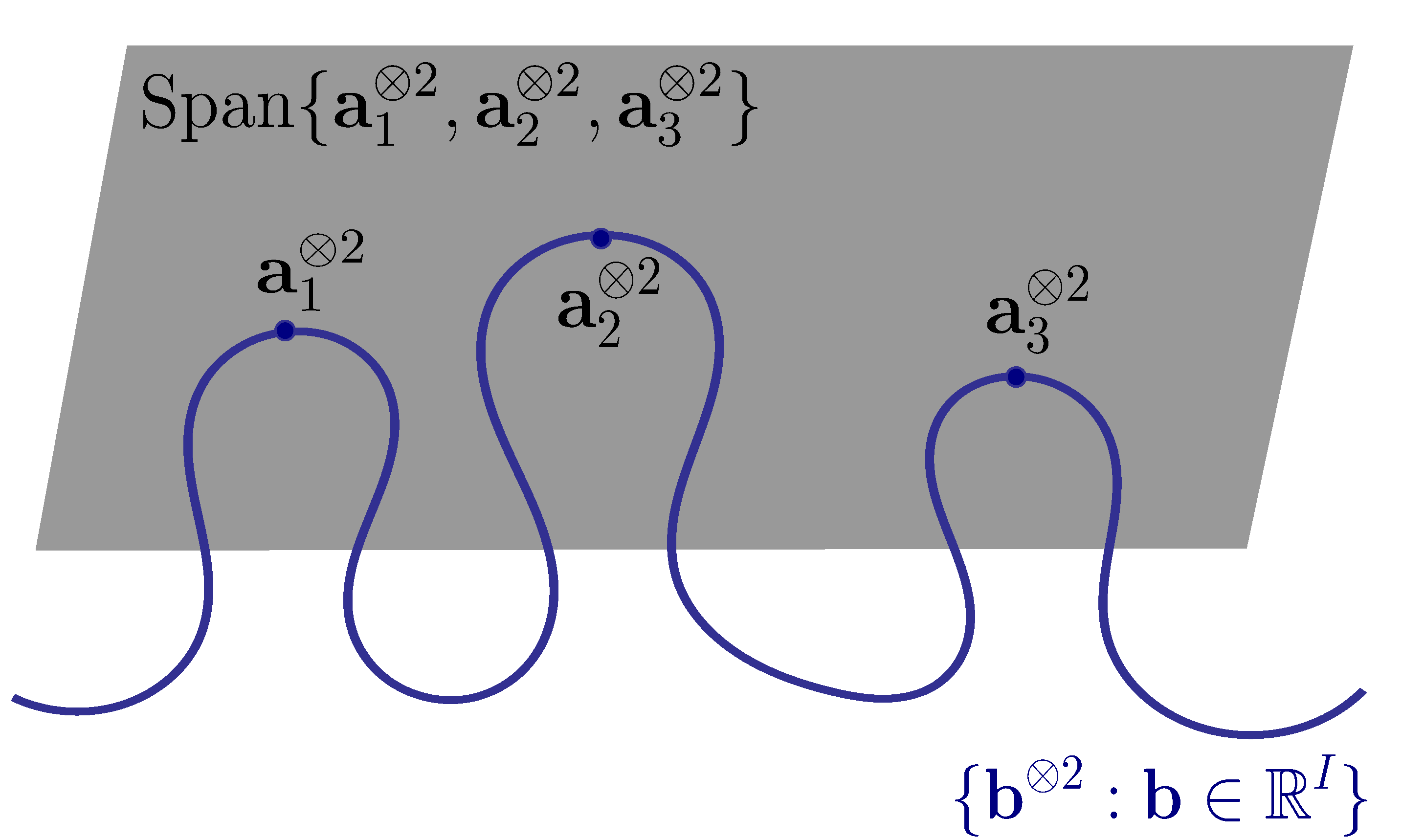
Figure 1: Illustration of Theorem 1.5

The $d$-th cumulant of a distribution on $\mathbb{R}^{I}$ is a symmetric order $d$ tensor of format $I\times\cdots\times I$ that encodes properties of the distribution [McC18, Chapter 2]. The $d$-th cumulant of $\mathbf{x}=A\mathbf{s}$ is

$$\kappa_{d}=\sum\limits_{j=1}^{J}\lambda_{j}\mathbf{a}_{j}^{\otimes d},$$

where $\mathbf{s}=(s_{1},\ldots,s_{J})$ has independent entries, the scalar $\lambda_{j}$ is the $d$-th cumulant of $s_{j}$, and $\mathbf{a}_{j}^{\otimes d}$ is the tensor with $(i_{1},\ldots,i_{d})$ entry $(\mathbf{a}_{j})_{i_{1}}\cdots(\mathbf{a}_{j})_{i_{d}}$. This follows from the fact that the cumulant tensor of a vector of independent entries is diagonal and from the multilinearity property of cumulants.

Theorem 1.5 may be surprising at first, since it only uses second order information about the matrix $A$. We might have expected a condition that involves terms $\mathbf{a}_{j}^{\otimes d}$ from higher-order cumulants. However, since for a Gaussian all cumulants of order greater than two are zero, our characterization turns out to only depend on the second powers $\mathbf{a}_{j}^{\otimes 2}$.

Theorem 1.5 implies the identifiability of square ICA, as follows.

Example 1.6.

Let $\mathbf{x}=A\mathbf{s}$, where $A\in\mathbb{R}^{I\times I}$ is invertible and $\mathbf{s}$ is a vector of independent sources with one source Gaussian. Assume there exists $\mathbf{b}\in\mathbb{R}^{I}$ with $\mathbf{b}^{\otimes 2}=\sum_{i=1}^{I}\lambda_{i}\mathbf{a}_{i}^{\otimes 2}$. After a change of basis, we have $(\mathbf{b}^{\prime})^{\otimes 2}=\sum_{i=1}^{I}\lambda_{i}\mathbf{e}_{i}^{\otimes 2}$, where the $\mathbf{e}_{i}$ are elementary basis vectors, since the columns $\mathbf{a}_{i}$ are linearly independent. Hence $\mathbf{b}^{\prime}$ is a diagonal rank one matrix. Therefore $\mathbf{b}^{\prime}$ is parallel to $\mathbf{e}_{i}$ for some $i$, so $\mathbf{b}$ is parallel to $\mathbf{a}_{i}$ for some $i$. The model is then identifiable, by Theorem 1.5.

The following examples illustrate Theorem 1.5 in overcomplete settings.

Example 1.7.

Consider the mixing matrix

$$A=\begin{pmatrix}1&0&0&0&1&0\\ 0&1&0&0&1&1\\ 0&0&1&0&1&1\\ 0&0&0&1&0&1\end{pmatrix}.$$ (2)

No pair of columns of $A$ are collinear. Let $\mathbf{b}^{\otimes 2}=\sum_{j=1}^{6}\lambda_{j}\mathbf{a}_{j}^{\otimes 2}$. Then

$$\mathbf{b}^{\otimes 2}=\begin{bmatrix}\lambda_{1}+\lambda_{5}&\lambda_{5}&\lambda_{5}&0\\ \lambda_{5}&\lambda_{2}+\lambda_{5}+\lambda_{6}&\lambda_{5}+\lambda_{6}&\lambda_{6}\\ \lambda_{5}&\lambda_{5}+\lambda_{6}&\lambda_{3}+\lambda_{5}+\lambda_{6}&\lambda_{6}\\ 0&\lambda_{6}&\lambda_{6}&\lambda_{4}+\lambda_{6}\end{bmatrix}.$$

The $2\times 2$ minors of this matrix vanish, since $\mathbf{b}^{\otimes 2}$ has rank one. This cannot happen unless all but one $\lambda_{i}$ is zero, as can be seen from a Macaulay2 [GS02] computation, so $\mathbf{b}$ is collinear to one of the $\mathbf{a}_{j}$. Hence $A$ is identifiable, by Theorem 1.5.

To explain the condition in Theorem 1.5, we show directly that $A$ is identifiable. To simplify our exposition, we assume that the non-Gaussian sources have non-vanishing fourth cumulants. Suppose $s_{1},\ldots,s_{5}$ are the non-Gaussian sources. A tensor of the form $\sum_{j=1}^{5}\lambda_{j}\mathbf{a}_{j}^{\otimes 4}$ has a unique tensor decomposition, by Kruskal’s criterion [Kru77]. Hence columns $\mathbf{a}_{1},\ldots,\mathbf{a}_{5}$ can be recovered uniquely, up to permutation and scaling. The covariance matrix of $A\mathbf{s}$ has the form $\sum_{j=1}^{6}\mu_{j}\mathbf{a}_{j}^{\otimes 2}$. If there are two candidates $\mathbf{a}_{6}$ and $\mathbf{b}$ for the last column, then $\mathbf{b}^{\otimes 2}\in\operatorname{Span}\{\mathbf{a}_{j}^{\otimes 2}:j=1,\ldots,6\}$.

Example 1.8.

The mixing matrix

$$A=\begin{pmatrix}1&0&1\\ 0&1&1\end{pmatrix}$$ (3)

does not satisfy the condition in Theorem 1.5, since $\mathbf{b}^{\otimes 2}=-(\mathbf{a}_{1})^{\otimes 2}+2(\mathbf{a}_{2})^{\otimes 2}+2(\mathbf{a}_{3})^{\otimes 2}$ holds for $\mathbf{b}=(1,2)$. Hence $A$ is non-identifiable. We exhibit the non-identifiability, as follows. Suppose $s_{1},s_{2},s_{3}$ follow exponential distributions with parameter $1$, that $r_{1},r_{2}$ follow standard Gaussian distributions, and that $s_{1},s_{2},s_{3},r_{1},r_{2}$ are independent. Then

$$\begin{pmatrix}1&0&1\\ 0&1&1\end{pmatrix}\begin{pmatrix}s_{1}\\ s_{2}-r_{1}+r_{2}\\ r_{1}+r_{2}\end{pmatrix}=\begin{pmatrix}1&0&1\\ 0&1&2\end{pmatrix}\begin{pmatrix}s_{1}+r_{1}\\ s_{2}\\ r_{2}\end{pmatrix}.$$

Both source vectors have independent entries with the last coordinate Gaussian, since $r_{1}+r_{2}$ and $-r_{1}+r_{2}$ are independent Gaussians.

Our second contribution characterizes whether a generic matrix $A\in\mathbb{R}^{I\times J}$ is identifiable. A generic matrix is one that lies outside of a set defined by the vanishing of some equations. In particular, genericity holds almost surely in $\mathbb{R}^{I\times J}$.

Theorem 1.9.

Let $A\in\mathbb{R}^{I\times J}$ be generic. Then

1. If $J\leq{I\choose 2}$ or if $(I,J)=(2,2)$ or $(3,4)$, then $A$ is identifiable;

2. If $J={I\choose 2}+1$, where $I\geq 4$ and $I\equiv 2,3\mod 4$, then there is positive probability that $A$ is identifiable and a positive probability that $A$ is non-identifiable;

3. If $J>{I\choose 2}+1$ or if $J={I\choose 2}+1$ and $I\equiv 0,1\mod 4$, then $A$ is non-identifiable.

To prove Theorem 1.9, we first studying the identifiability condition in Theorem 1.5 over the complex numbers. Then we specialize to the real numbers, proving the following. No extra complex solutions implies no extra real solutions. If there are a finite number $k$ of extra complex solutions, the presence of extra real solutions depends on the parity of $k$: if odd, there is an extra solution, but if even, there may or may not be. If there are infinitely many extra complex solutions, then we show that there is an extra real solution.

Our third contribution is an algorithm to recover the mixing matrix $A\in\mathbb{R}^{I\times J}$, via tensor decomposition. ICA has close connections to tensor decomposition. Comon explained how to obtain the mixing matrix from the higher order cumulant tensors of the observed variables [Com94]. When the sources are non-Gaussian and the number of sources is at most the number of observations, tensor algorithms include JADE [CS93], which uses fourth order cumulants, STOTD [DLDMV01], which uses third order cumulants, and algorithms that combine cumulants of different orders [Mor01]. For overcomplete ICA, algorithms include FOOBI [DLCC07], which uses fourth order cumulants and BIRTH, which uses hexacovariance (the flattening of the six order cumulant) [ACCF04]. However, to our knowledge, there do not exist algorithms that apply to the setting where one of the sources is Gaussian. Having a Gaussian source is natural to represent noise or, in practice, to allow sources that are close to Gaussian [SHMF14].

Algorithm 1 Recover $A$ from the second and fourth order cumulants of $\mathbf{x}$

1:Second and fourth order cumulants $\kappa_{2},\kappa_{4}$ of $\mathbf{x}=A\mathbf{s}$ for matrix $A\in\mathbb{R}^{I\times J}$ and independent sources $\mathbf{s}$ with one Gaussian $s_{J}$.

2:The first $J-1$ columns of $A$: Compute the symmetric tensor decomposition of $\kappa_{4}$ to recover $\mathbf{a}_{1},\ldots,\mathbf{a}_{J-1}$, up to permutation and scaling.

3:The last column of $A$: Find a rank one matrix in $\operatorname{Span}\{\mathbf{a}_{1}^{\otimes 2},\ldots,\mathbf{a}_{J-1}^{\otimes 2},\kappa_{2}\}$ that is not collinear to $\mathbf{a}_{1}^{\otimes 2},\ldots,\mathbf{a}_{J-1}^{\otimes 2}$, by initializing at a random rank one matrix and a random point in the span and minimizing the distance between them using Powell’s method [Pow64].

4:Matrix $A\in\mathbb{R}^{I\times J}$ with columns $\mathbf{a}_{1},\ldots,\mathbf{a}_{J}$.

Our algorithm uses [KP19, Algorithm 1] in the first step. We could, in principle, use any tensor decomposition algorithm here. We use this method because of its compatibility with our second step: both look for rank one matrices or tensors in a linear space.

We apply our algorithm to synthetic data, where it corroborates our identifiability results, to the CIFAR-10 dataset [KNH14] of images, to incorporate Gaussian noise into bases of image patches, cf. [PPW⁺19], and to protein signalling [SPP⁺05], to incorporate Gaussian noise into the causal structure learning algorithm of [SHH⁺06].

The rest of the paper is organized as follows. We prove Theorem 1.5 in Section 2. We relate identifiability to systems of quadrics in Section 3 and study these quadrics in Section 4. We prove Theorem 1.9 in Section 5. We study the identifiability of special matrices in Section 6. Our numerical results are in Section 7.

2 Characterization of identifiability

We prove Theorem 1.5, our characterization of the identifiability of ICA.

2.1 Sufficiency

We show that the condition of Theorem 1.5 is sufficient for identifiability of ICA.

Proposition 2.1.

Fix $A\in\mathbb{R}^{I\times J}$ with columns $\mathbf{a}_{1},\ldots,\mathbf{a}_{J}$, and no pair of columns collinear. Then $A$ is identifiable if the linear span of the rank one matrices $\mathbf{a}_{1}^{\otimes 2},\ldots,\mathbf{a}_{J}^{\otimes 2}$ does not contain any real rank one matrix $\mathbf{b}^{\otimes 2}$, unless $\mathbf{b}$ is collinear to $\mathbf{a}_{j}$ for some $j\in\{1,\ldots,J\}$.

For the proof, we use the second characteristic function, the cumulant generating function. We also use the following results: Theorem 2.2 relates the second characteristic function of a linear mixing to its sources, Theorem 2.3 settles the uniqueness of the mixing matrix of the non-Gaussian sources, and Theorem 2.4 turns the study of second characteristic functions into degree two equations.

Theorem 2.2 ([CJ10, Proposition 9.4]).

Let $\mathbf{x}=A\mathbf{s}$ with the entries of $\mathbf{s}$ independent. Then

$$\Psi_{\mathbf{x}}(\mathbf{u})=\sum_{j=1}^{J}\Psi_{s_{j}}(\mathbf{u}^{\mathsf{T}}\mathbf{a}_{j}),$$

in a neighbourhood of the origin, where $\Psi_{\mathbf{x}}$ and $\Psi_{s_{j}}$ are the second characteristic functions of the random variables $\mathbf{x}$ and $s_{j}$.

Theorem 2.3 (See [CJ10, Theorem 9.1] and [KLR73, Theorem 10.3.1]).

Let $\mathbf{x}=A\mathbf{s}$, where $s_{j}$ are independent and non-degenerate and $A$ does not have any collinear columns. Then $\mathbf{x}=A_{1}\mathbf{s_{1}}+A_{2}\mathbf{s_{2}}$, where $\mathbf{s_{1}}$ is a vector of non-Gaussian, $\mathbf{s_{2}}$ is a vector of Gaussian and independent of $\mathbf{s_{1}}$, and $A_{1}$ is unique, up to permuting and scaling of its columns.

Theorem 2.4 ([KLR73, Lemma A.2.4]).

Fix vectors $\mathbf{\alpha}_{1},\ldots,\mathbf{\alpha}_{n}\in\mathbb{R}^{p}$ and a vector of variables $\mathbf{u}:=(u_{1},\ldots,u_{p})^{\mathsf{T}}$. Assume that $\alpha_{i}$ is not collinear to $\alpha_{j}$ for $i\neq j$ or to any elementary basis vector. Let $\psi_{1},\ldots,\psi_{n},A_{1},\ldots,A_{p}$ be complex-valued continuous functions. Assume that

$$\psi_{1}(\alpha_{1}^{\mathsf{T}}\mathbf{u})+\cdots+\psi_{n}(\alpha_{n}^{\mathsf{T}}\mathbf{u})=\sum_{i=1}^{p}A_{i}(u_{i})+P_{k}(\mathbf{u}),$$

for all $\mathbf{u}$ in a neighborhood of the origin, where $P_{k}$ is a degree $k$ polynomial in $\mathbf{u}$. Then the functions $\psi_{j}$ and $A_{i}$ are all polynomials of degree at most $\max\{n,k\}$ in an interval around the origin.

Proof of Proposition 2.1.

The model $\mathbf{x}=A\mathbf{s}$ is identifiable when $\mathbf{s}$ does not contain a Gaussian, by [EK04, Theorem 3], since $A$ has no pair of columns collinear. It remains to consider the case that $\mathbf{s}$ contains one Gaussian. Without loss of generality, suppose that $s_{J}$ is standard Gaussian. Take $B\in\mathbb{R}^{I\times K}$ with $K\leq J$ and $\mathbf{r}=(r_{1},\ldots,r_{K})$ with $B\mathbf{r}=\mathbf{x}$. The columns of $B$ corresponding to non-Gaussian sources must each be collinear to one of $\mathbf{a}_{1},\ldots,\mathbf{a}_{J-1}$, by Theorem 2.3. The vectors $\mathbf{r}$ and $\mathbf{s}$ have the same number of Gaussian entries. The number of non-Gaussian and Gaussian sources in $\mathbf{r}$ must then be $J-1$ and $1$ respectively, by Theorem 2.3 and the assumption $K\leq J$. Without loss of generality, assume that $r_{J}$ is a standard Gaussian. Then the first $J-1$ columns of $B$ equal the first $J-1$ columns of $A$, up to scaling and permutation, by Theorem 2.3. Denote the last column of $B$ by $\mathbf{b}$.

The second characteristic function of a standard Gaussian $x$ is $\Psi_{x}(t)=-\frac{1}{2}t^{2}$. We have the equality

$$\sum_{j=1}^{J-1}(\Psi_{s_{j}}-\Psi_{r_{j}})(\mathbf{u}^{\mathsf{T}}\mathbf{a}_{j})-\frac{1}{2}(\mathbf{u}^{\mathsf{T}}\mathbf{a}_{J})^{2}+\frac{1}{2}(\mathbf{u}^{\mathsf{T}}\mathbf{b})^{2}=0,$$ (4)

by Theorem 2.2. We apply Theorem 2.4 to the functions $\psi_{j}=\Psi_{s_{j}}-\Psi_{r_{j}},A_{i}=0,P_{k}=\frac{1}{2}(\mathbf{u}^{\mathsf{T}}\mathbf{a}_{J})^{2}-\frac{1}{2}(\mathbf{u}^{\mathsf{T}}\mathbf{b})^{2}$. It shows that $\Psi_{s_{j}}-\Psi_{r_{j}}$ is polynomial in a neighborhood of the origin, for all $1\leq j\leq J-1$. Taking the degree two part of (4), we obtain an identity $\sum_{j=1}^{J-1}\lambda_{j}(\mathbf{u}^{\mathsf{T}}\mathbf{a}_{j})^{2}+(\mathbf{u}^{\mathsf{T}}\mathbf{a}_{J})^{2}-(\mathbf{u}^{\mathsf{T}}\mathbf{b})^{2}=0$, for some scalars $\lambda_{1},\ldots,\lambda_{J-1}$. That is,

$$\mathbf{b}^{\otimes 2}=\mathbf{a}_{J}^{\otimes 2}+\sum_{j=1}^{J-1}\lambda_{j}\mathbf{a}_{j}^{\otimes 2}.$$

By the condition in the statement, we conclude that $\mathbf{b}$ is collinear to $\mathbf{a}_{j}$ for some $j=1,\ldots,J$. However, $\mathbf{b}$ is not collinear to the first $J-1$ columns of $B$, since $B$ has no pair of columns collinear. Hence, it is not collinear to the first $J-1$ columns of $A$, and therefore $\mathbf{b}$ is collinear to $\mathbf{a}_{J}$. Hence $A$ and $B$ are equal, up to permutation and scaling of columns. ∎

Taking the degree two part of (4) requires Theorem 2.4: in general, second characteristic functions may not have Taylor expansions. We now show how Proposition 2.1 suggests the viability of Algorithm 1.

Theorem 2.5.

Fix $J\leq{I\choose 2}$. Suppose we have a generic $A\in\mathbb{R}^{I\times J}$ satisfying the condition in Theorem 1.5 and a system of independent sources $\mathbf{s}$ with one Gaussian and the rest non-Gaussian with non-vanishing second and fourth cumulants. Then $A$ can be recovered, up to permutation and scaling of its columns, from the second and fourth cumulants of $A\mathbf{s}$.

Proof.

Without loss of generality, suppose that $s_{J}$ is the Gaussian source. Let the fourth cumulant of $s_{j}$ be $\lambda_{j}\in\mathbb{R}\backslash\{0\}$. Then the fourth cumulant tensor of $\mathbf{x}=A\mathbf{s}$ is $\kappa_{4}=\sum_{j=1}^{J-1}\lambda_{j}\mathbf{a}_{j}^{\otimes 4}$. The rank is $J-1$, by the genericity of the vectors $\mathbf{a}_{j}$. A generic symmetric tensor of format $I\times I\times I\times I$ has symmetric rank $\lceil\frac{1}{24}(I+3)(I+2)(I+1)\rceil$, by the Alexander-Hirschowitz Theorem [JA95]. The rank of $\kappa_{4}$ is less than the generic rank, since $J-1\leq{{I\choose 2}}$ and the inequality ${I\choose 2}<\lceil\frac{1}{24}(I+3)(I+2)(I+1)\rceil$ holds for all $I$. Hence $\kappa_{4}$ has a unique symmetric decomposition, by [COV17, Theorem 1.1]. Therefore, the first $J-1$ columns of $A$ can be recovered, up to scaling and permutation, via the symmetric tensor decomposition of $\kappa_{4}$.

The second cumulant of $\mathbf{x}$ is $\kappa_{2}=\sum_{j=1}^{J}\mu_{k}\mathbf{a}_{j}\otimes\mathbf{a}_{j}$, where $\mu_{j}$ is the variance of $s_{j}$. Hence $\operatorname{Span}\{\mathbf{a}_{1}^{\otimes 2},\ldots,\mathbf{a}_{J-1}^{\otimes 2},\kappa_{2}\}=\operatorname{Span}\{\mathbf{a}_{1}^{\otimes 2},\ldots,\mathbf{a}_{J}^{\otimes 2}\}$. By assumption, the only real rank one matrices in $\operatorname{Span}\{\mathbf{a}_{1}^{\otimes 2},\ldots,\mathbf{a}_{J}^{\otimes 2}\}$ are $\mathbf{a}_{1}^{\otimes 2},\ldots,\mathbf{a}_{J}^{\otimes 2}$ up to scalar, so a rank one matrix $\mathbf{a}_{J}^{\otimes 2}$ in $\operatorname{Span}\{\mathbf{a}_{1}^{\otimes 2},\ldots,\mathbf{a}_{J-1}^{\otimes 2},\kappa_{2}\}$ that is not collinear to $\mathbf{a}_{1}^{\otimes 2},\ldots,\mathbf{a}_{J-1}^{\otimes 2}$ must be a scalar multiple of $\mathbf{a}_{J}^{\otimes 2}$. Hence, $A$ is recovered uniquely up to column permutation and scaling from the second and fourth cumulant tensors of $A\mathbf{s}$. ∎

2.2 Necessity

We complete the proof of Theorem 1.5, showing that our condition is necessary.

Proposition 2.6.

Fix matrix $A\in\mathbb{R}^{I\times J}$ with columns $\mathbf{a}_{1},\ldots,\mathbf{a}_{J}$. Then $A$ is identifiable only if no pair of its columns is collinear and the linear span of $\mathbf{a}_{1}^{\otimes 2},\ldots,\mathbf{a}_{J}^{\otimes 2}$ does not contain any real matrix $\mathbf{b}^{\otimes 2}$ unless $\mathbf{b}$ is collinear to $\mathbf{a}_{j}$ for some $j\in\{1,\ldots,J\}$.

Proof.

If the mixing matrix $A$ has two collinear columns, we can combine them and obtain a matrix $B\in\mathbb{R}^{I\times(J-1)}$ and a system of independent sources $\mathbf{r}=(r_{1},\ldots,r_{J-1})$ such that $B\mathbf{r}$ and $A\mathbf{x}$ have the same distribution. Hence identifiability implies no pair of collinear columns.

Assume there exists $\mathbf{b}^{\otimes 2}\in\operatorname{Span}\{\mathbf{a}_{1}^{\otimes 2},\ldots,\mathbf{a}_{J}^{\otimes 2}\}$ with $\mathbf{b}$ not collinear to any $\mathbf{a}_{j}$. Then

$$\mathbf{b}^{\otimes 2}=\sum_{j=1}^{J-1}\lambda_{j}\mathbf{a}_{j}^{\otimes 2}+\mathbf{a}_{J}^{\otimes 2},$$

since we can assume without loss of generality that the coefficient of $\mathbf{a}_{J}$ is one. Let $B$ be the matrix with columns $\mathbf{a}_{1},\ldots,\mathbf{a}_{J-1},\mathbf{b}$. We will construct independent random variables $s_{j}$ and $r_{j}$ such that $A\mathbf{s}$ and $B\mathbf{r}$ have the same distribution.

Let $r_{J}$ and $s_{J}$ be standard Gaussians. Choose $J-1$ non-Gaussian random variables $y_{1},\ldots,y_{J-1}$ and Gaussian distributions $z_{1},\ldots,z_{J-1}$ with second characteristic functions

$$\Psi_{z_{j}}(t)=\begin{cases}-\frac{1}{2}|\lambda_{j}|t^{2}&\lambda_{j}\neq 0\\ 0&\lambda_{j}=0,\end{cases}$$

such that these random variables together with the standard Gaussians $r_{J},s_{J}$ are independent. When $\lambda_{j}\geq 0$, set $r_{j}=y_{j}$ and $s_{j}=y_{j}+z_{j}$; when $\lambda_{j}<0$, set $s_{j}=y_{j}$ and $r_{j}=y_{j}+z_{j}$. Then $s_{1},\ldots,s_{J}$ are independent and $r_{1},\ldots,r_{J}$ are independent. The source variables differ by Gaussians. We have

$$(\Psi_{s_{j}}-\Psi_{r_{j}})(t)=\begin{cases}(\Psi_{y_{j}+z_{j}}-\Psi_{y_{j}})(t)&\lambda_{j}>0\\ (\Psi_{y_{j}}-\Psi_{y_{j}+z_{j}})(t)&\lambda_{j}<0\\ 0&\lambda_{j}=0.\end{cases}$$

All three cases evaluate to give $(\Psi_{s_{j}}-\Psi_{r_{j}})(t)=-\frac{1}{2}\lambda_{j}t^{2}$. The second characteristic functions of $A\mathbf{s},B\mathbf{r}$ are equal, by Theorem 2.2, since

$$\Psi_{A\mathbf{s}}(\mathbf{u})-\Psi_{B\mathbf{r}}(\mathbf{u})=\sum_{j=1}^{J-1}(\Psi_{s_{j}}-\Psi_{r_{j}})(\mathbf{u}^{\mathsf{T}}\mathbf{a}_{j})-\frac{1}{2}(\mathbf{u}^{\mathsf{T}}\mathbf{a}_{J})^{2}+\frac{1}{2}(\mathbf{u}^{\mathsf{T}}\mathbf{b})^{2}=0.$$ (5)

Hence $A\mathbf{s}$ and $B\mathbf{r}$ have the same distribution. The last column of $B$ is not collinear to any column of $A$, so $A$ is not identifiable. ∎

Propositions 2.1 and 2.6 combine to prove Theorem 1.5. We give an example of a identifiable matrix $A$. We build such examples in Section 6.

Example 2.7.

Let

$$A=\begin{pmatrix}0&3&1&\frac{-27417}{160871}&1&0&0&0\\ 1&9&11&\frac{282663}{36181}&0&1&0&0\\ 2&14&13&17&0&0&1&0\\ 3&1&\frac{-89735}{6339}&19&0&0&0&1\end{pmatrix}.$$

If $\mathbf{b}^{\otimes 2}\in\operatorname{Span}\{\mathbf{a}_{1}^{\otimes 2},\ldots,\mathbf{a}_{8}^{\otimes 2}\}$, then $\mathbf{b}$ collinear to $\mathbf{a}_{j}$ for some $j\in\{1,\ldots,8\}$, as can be checked in Macaulay2. So $A$ is identifiable, by Theorem 1.5.

3 From identifiability to systems of quadrics

The characterization of identifiability in Theorem 1.5 is closely related to the study of systems of quadrics, as we now describe. We will use systems of quadrics to prove Theorem 1.9. The proof has two steps. The first step is to study the complex analogue of identifiability. The second step is to convert the complex results into real insights for the real setting of ICA. We give the complex analogue of Definition 1.3.

Definition 3.1.

A mixing matrix $A\in\mathbb{C}^{I\times J}$ is complex identifiable if for any non-degenerate sources $\mathbf{s}=(s_{1},\ldots,s_{J})^{\mathsf{T}}$ with at most one $s_{j}$ Gaussian, matrix $A$ can be recovered uniquely, up to permutation and scaling of its columns, from $A\mathbf{s}$. That is, if $A\mathbf{s}$ and $B\mathbf{r}$ have the same distribution for some $B\in\mathbb{C}^{I\times K}$ with $K\leq J$ and some $\mathbf{r}=(r_{1},\ldots,r_{K})$, with the same number of Gaussian entries as $\mathbf{s}$, then $J=K$ and matrices $A$ and $B$ coincide, up to permutation and scaling of columns.

Complex ICA appears in applications to telecommunications [UAIN15] and in ICA algorithms such as [DLCC07] and [ACCF04]. We prove the complex analogue of Theorem 1.5.

Proposition 3.2.

A matrix $A\in\mathbb{C}^{I\times J}$ is complex identifiable if and only if no pair of its columns are collinear and the linear span of the matrices $\mathbf{a}_{1}^{\otimes 2},\ldots,,\mathbf{a}_{J}^{\otimes 2}$ does not contain any rank one matrix that is not collinear to $\mathbf{a}_{1}^{\otimes 2},\ldots,\mathbf{a}_{J}^{\otimes 2}$.

Proof.

The sufficient direction is the same as the proof of Proposition 2.1. For the necessary direction, the proof is simpler than Proposition 2.6, since we allow complex square roots. The matrix $A$ cannot have collinear columns, as in Proposition 2.6. Given $\mathbf{b}^{\otimes 2}\in\operatorname{Span}\{\mathbf{a}_{j}^{\otimes 2}:j=1,\ldots,J\}$ such that $\mathbf{b}$ is not collinear to any $\mathbf{a}_{j}$, we write

$$\mathbf{b}^{\otimes 2}=\sum_{j=1}^{J-1}\lambda_{j}\mathbf{a}_{j}^{\otimes 2}+\mathbf{a}_{J}^{\otimes 2},$$

since we can assume without loss of generality that the coefficient of $\mathbf{a}_{J}$ is one. Define $A$ and $B$ as in the proof of Proposition 2.6. Let $r_{J}$ and $s_{J}$ be standard Gaussians. Choose $J-1$ non-Gaussian random variables $y_{1},\ldots,y_{J-1}$ and standard Gaussian distributions $z_{1},\ldots,z_{J-1}$. Define $r_{j}=y_{j}$ and $s_{j}=y_{j}+\sqrt{\lambda_{j}}z_{j}$. Then $\Psi_{s_{j}}(t)=\Psi_{y_{j}}(t)+\lambda_{j}\Psi_{z_{j}}(t)$. The source variables differ by a complex scalar multiple of a Gaussian. The second characteristic functions for $A\mathbf{s}$ and $B\mathbf{r}$ are equal, by Theorem 2.2, since

$$\Psi_{A\mathbf{s}}(\mathbf{u})-\Psi_{B\mathbf{r}}(\mathbf{u})=\sum_{j=1}^{J-1}(\Psi_{s_{j}}-\Psi_{r_{j}})(\sum_{i=1}^{I}u_{i}a_{ij})-\frac{1}{2}(\sum_{i=1}^{I}u_{i}a_{iJ})^{2}+\frac{1}{2}(\sum_{i=1}^{I}u_{i}b_{i})^{2}=0.$$ (6)

Hence $A\mathbf{s}$ and $B\mathbf{r}$ have the same distribution. The last column of $B$ is not collinear to any column of $A$, so $A$ is not complex identifiable. ∎

We will prove the following characterization of complex identifiability.

Theorem 3.3.

Let $A\in\mathbb{C}^{I\times J}$ be generic. Then

1. If $J\leq{I\choose 2}$ or if $(I,J)=(2,2)$ or $(3,4)$, then $A$ is complex identifiable;

2. If $J\geq{I\choose 2}+2$ or if $J\geq{I\choose 2}+1$ for $I\geq 4$, then $A$ is complex non-identifiable.

Theorem 3.3 immediately implies part 1 of Theorem 1.9.

Corollary 3.4.

Let $A\in\mathbb{R}^{I\times J}$ be generic. If $J\leq{I\choose 2}$ or if $(I,J)=(2,2)$ or $(3,4)$, then $A$ is identifiable.

Proof.

Such matrices $A$ are complex identifiable, by Theorem 3.3. Hence no pair of its columns are collinear and the linear span of $\mathbf{a}_{1}^{\otimes 2},\ldots,\mathbf{a}_{J}^{\otimes 2}$ does not contain any rank one matrix not collinear to $\mathbf{a}_{1}^{\otimes 2},\ldots,\mathbf{a}_{J}^{\otimes 2}$, by Proposition 3.2. In particular, the linear span contains no real rank one matrix. Hence $A$ is identifiable, by Theorem 1.5. ∎

Theorem 1.5 and Proposition 3.2 translate to conditions on systems of quadrics, homogeneous degree two polynomials, as we now explain. Theorem 1.5 involves the linear space $\operatorname{Span}\{\mathbf{a}_{j}^{\otimes 2}:j=1,\ldots,J\}$. We view a symmetric matrix $M$ either as an array of $I\times I$ entries $M_{ij}$, for $1\leq i,j\leq I$, or as a vector of ${I+1\choose 2}$ entries $M_{ij}$, for $1\leq i\leq j\leq I$. In our identifiability conditions, two vectors or matrices are equivalent if they agree up to scale, so it is convenient to work in projective space. We denote the projectivization of $\operatorname{Span}\{\mathbf{a}_{j}^{\otimes 2}:j=1,\ldots,J\}$ by $\mathcal{W}(A)$. It is a linear space in $\mathbb{P}_{\mathbb{C}}^{m-1}$, where $m={I+1\choose 2}$. The coordinates on $\mathbb{P}_{\mathbb{C}}^{m-1}$ are $\mathbf{z}=(z_{ij}:1\leq i\leq j\leq I)$. The space $\mathcal{W}(A)$ is defined by linear relations

$$l_{1}(\mathbf{z})=\sum\limits_{1\leq i\leq j\leq I}\lambda^{(1)}_{ij}z_{ij}\quad\ldots\quad l_{k}(\mathbf{z})=\sum\limits_{1\leq i\leq j\leq I}\lambda^{(k)}_{ij}z_{ij}.$$ (7)

The number of quadrics $k$ is the number of linearly independent conditions that cut out $\mathcal{W}(A)$. In particular, if $\mathcal{W}(A)$ spans the whole space then $k=0$. We study rank one matrices in $\mathcal{W}(A)$. The projectivization of the set of rank one $I\times I$ symmetric matrices is the second Veronese embedding of $\mathbb{P}_{\mathbb{C}}^{I-1}$. We denote it by $\mathcal{V}_{I}$. It is the image of the map

$$\phi:\mathbb{P}_{\mathbb{C}}^{I-1} \to\mathbb{P}_{\mathbb{C}}^{m-1}$$

$$[x_{1}:\ldots:x_{I}] \mapsto[x_{1}^{2}:x_{1}x_{2}:\ldots:x_{I}^{2}],$$

see [Har92, Exercise 2.8 and Example 18.13]. The intersection $\mathcal{V}_{I}\cap\mathcal{W}(A)$ consists of all rank one matrices, up to scale, that lie in $\operatorname{Span}\{\mathbf{a}_{j}^{\otimes 2}:j=1,\ldots,J\}$. In particular, it contains $\mathbf{a}_{1}^{\otimes 2},\ldots,\mathbf{a}_{J}^{\otimes 2}$. The rank one condition converts (7) into the system of quadrics

$$f_{1}(\mathbf{x})=\sum\limits_{1\leq i\leq j\leq I}\lambda^{(1)}_{ij}x_{i}x_{j}\quad\ldots\quad f_{k}(\mathbf{x})=\sum\limits_{1\leq i\leq j\leq I}\lambda^{(k)}_{ij}x_{i}x_{j}.$$ (8)

The intersection $\mathcal{V}_{I}\cap\mathcal{W}(A)$ is the vanishing locus of the quadrics $f_{1},\ldots,f_{k}$, which we denote by $V(f_{1},\ldots,f_{k})$. We say $\{f_{1},\ldots,f_{k}\}$ is a system of quadrics defining $\mathcal{V}_{I}\cap\mathcal{W}(A)$. Proposition 3.2 says that $A$ is complex identifiable if and only if $V(f_{1},\ldots,f_{k})=\{\mathbf{a}_{1}^{\otimes 2},\ldots,\mathbf{a}_{J}^{\otimes 2}\}$. Theorem 1.5 says that $A$ is identifiable if and only if $V(f_{1},\ldots,f_{k})$ does not contain any real points other than $\mathbf{a}_{1}^{\otimes 2},\ldots,\mathbf{a}_{J}^{\otimes 2}$.

Example 3.5.

Let $A$ be the matrix from Example 1.7. The linear equations defining $\mathcal{W}(A)$ are the rows of the matrix

$$\pNiceMatrix[first-row]z_{11}&z_{12}z_{13}z_{14}z_{22}z_{23}z_{24}z_{33}z_{34}z_{44}\\ 01000-11000\\ 00100-11000\\ 01000-10010\\ 0001000000\\ .$$

The corresponding system of quadrics defining $\mathcal{V}_{I}\cap\mathcal{W}(A)$ is obtained by replacing $z_{ij}$ by $x_{i}x_{j}$, to give $f_{1}=x_{1}x_{2}-x_{2}x_{3}+x_{2}x_{4}$, $f_{2}=x_{1}x_{3}-x_{2}x_{3}+x_{2}x_{4}$, $f_{3}=x_{1}x_{2}-x_{2}x_{3}+x_{3}x_{4}$, $f_{4}=x_{1}x_{4}$.

4 Systems of quadrics

Quadrics have been studied as far back as 300BC [Hea21]. They remain a popular topic in algebraic geometry, see e.g. [BKT08, OSG20, FMS20]. In this section, we prove results for systems of quadrics, which may be of independent interest, and which are building blocks of our proof of Theorem 1.9. We prove the following quadric restatement of Theorem 3.3 in Section 4.1. The case $J\leq{I\choose 2}$ is [KP19, Proposition 3.2].

Theorem 4.1.

Let $\mathcal{V}_{I}$ be the second Veronese embedding of $\mathbb{P}_{\mathbb{C}}^{I-1}$. Suppose that $\mathbf{v}_{1}^{\otimes 2},\ldots,\mathbf{v}_{J}^{\otimes 2}$ are generic points on $\mathcal{V}_{I}$ with $\mathcal{W}(A)$ their projective linear span. Let the system of quadrics defining $\mathcal{V}_{I}\cap\mathcal{W}(A)$ be $\{f_{1},\ldots,f_{k}\}$, with vanishing locus $V(f_{1},\ldots,f_{k})$.

1. If $J\leq{I\choose 2}$ or if $(I,J)=(2,2)$ or $(3,4)$, then $V(f_{1},\ldots,f_{k})=\{\mathbf{v}_{1}^{\otimes 2},\ldots,\mathbf{v}_{J}^{\otimes 2}\}.$

2. If $J>{I\choose 2}+1$ or if $J>{I\choose 2}$ for $I\geq 4$, then $V(f_{1},\ldots,f_{k})\supsetneqq\{\mathbf{v}_{1}^{\otimes 2},\ldots,\mathbf{v}_{J}^{\otimes 2}\}.$

Example 4.2.

We revisit Examples 1.7 and 3.5. A Macaulay2 computation [GS02] confirms that $V(f_{1},f_{2},f_{3},f_{4})=\{\mathbf{a}_{1}^{\otimes 2},\ldots,\mathbf{a}_{6}^{\otimes 2}\}$, which proves that $A$ is complex identifiable (and, in particular, identifiable), by Theorem 4.1.

We prove the following result in Section 4.2. It is used in the identifiability result for $J={I\choose 2}+1$ in Theorem 1.9. By an open set of systems of $I-1$ quadrics, we mean the coefficients of the quadrics form an open set in the space of $(I-1){I+1\choose 2}$ coefficients.

Theorem 4.3.

For every even integer $\ell$ from $0$ to $2^{I-1}$, there is an open set of systems of $I-1$ quadrics in $\mathbb{R}[x_{1},\ldots,x_{I}]$ that have $2^{I-1}$ distinct intersection points, of which $\ell$ are real.

4.1 Complex solutions to a system of quadrics

In this section, we prove Theorems 4.1 and 3.3. As above, let $\mathcal{V}_{I}$ denote the second Veronese embedding of $\mathbb{P}_{\mathbb{C}}^{I-1}$ in $\mathbb{P}_{\mathbb{C}}^{m-1}$, where $m={I+1\choose 2}$.

Lemma 4.4.

Let $\mathbf{v}_{1}^{\otimes 2},\ldots,\mathbf{v}_{J}^{\otimes 2}$ be generic points of $\mathcal{V}_{I}$. Then the matrix in $\mathbb{C}^{{{I+1}\choose 2}\times J}$ with columns $\mathbf{v}_{1}^{\otimes 2},\ldots,\mathbf{v}_{J}^{\otimes 2}$ has full rank.

Proof.

The highest rank is attained for generic matrices, so it suffices to exhibit an example with full rank. Suppose $\mathbf{e}_{1},\ldots,\mathbf{e}_{I}$ are canonical basis vectors in $\mathbb{C}^{I}$. Let $S=\{\mathbf{e}_{1}^{\otimes 2},\ldots,\mathbf{e}_{I}^{\otimes 2}\}\cup\{(\mathbf{e}_{i}+\mathbf{e}_{j})^{\otimes 2}:i<j\}$. Then $|S|=m={{I+1\choose 2}}$. A subset of $S$ of size $J\leq m$ is linearly independent. When $J>m$, taking the union of $S$ with any $J-m$ symmetric rank one matrices forms a linear space of dimension $m$. In both cases, the matrix has full rank. ∎

Lemma 4.5.

For ${I\choose 2}+1$ generic points in $\mathcal{V}_{I}$, with span $\mathcal{W}$, the intersection $\mathcal{V}_{I}\cap\mathcal{W}$ consists of $2^{I-1}$ distinct points.

Proof.

The variety $\mathcal{V}_{I}$ has dimension $I-1$ and degree $2^{I-1}$ [Har92, Exercise 2.8 and Example 18.13]. A generic linear space of codimension $I-1$ therefore intersects $\mathcal{V}_{I}$ in $2^{I-1}$ distinct points, by Bézout’s Theorem. Our goal is to show that $\mathcal{W}$ from the statement is sufficiently generic: a codimension $I-1$ subspace that intersects $\mathcal{V}_{I}$ in degree many distinct points.

Let $J={I\choose 2}+1$ and $m={{I+1\choose 2}}$. The space $\mathcal{W}$ is spanned by $J$ points, and lives in $\mathbb{P}_{\mathbb{C}}^{m-1}$. It has projective dimension $(J-1)$, by Lemma 4.4. Hence it has codimension $I-1$, since $(I-1)+(J-1)=m-1$. That is, for generic $\mathbf{v}_{1},\ldots,\mathbf{v}_{J}\in\mathbb{P}_{\mathbb{C}}^{I-1}$, the projective linear space $\operatorname{Span}\{\mathbf{v}_{1}^{\otimes 2},\ldots,\mathbf{v}_{J}^{\otimes 2}\}$ is an element of the Grassmannian variety of $(J-1)$-dimensional projective linear spaces in $\mathbb{P}_{\mathbb{C}}^{m-1}$, which we denote $\operatorname{Gr}(J-1,m-1)$.

Let $\mathcal{U}\subset\operatorname{Gr}(J-1,m-1)$ be the set of spaces spanned by $J$ points on $\mathcal{V}_{I}$. The set $\mathcal{U}$ is open and dense in $\operatorname{Gr}(J-1,m-1)$, as follows. For a generic $(J-1)$-dimensional linear space $\mathcal{L}$, the intersection $\mathcal{V}_{I}\cap\mathcal{L}$ spans $\mathcal{L}$, by [Har92, Proposition 18.10] applied $I-1$ times, since the variety $\mathcal{V}_{I}$ is irreducible and non-degenerate (not contained in any hyperplane) and its generic hyperplane sections are also non-degenerate and irreducible if $\dim\mathcal{V}_{I}\geq 2$. Choosing a basis of $\mathcal{L}$ from $\mathcal{V}_{I}\cap\mathcal{L}$ shows that $\mathcal{U}$ is open and dense.

Let $\mathcal{U}^{\prime}$ denote the elements of $\operatorname{Gr}(J-1,m-1)$ that intersect $\mathcal{V}_{I}$ in degree many distinct points. Then $\mathcal{U}^{\prime}$ is open and dense, by Bézout’s theorem. Hence $\mathcal{U}\cap\mathcal{U}^{\prime}$ is open and dense in $\operatorname{Gr}(J-1,m-1)$. Define the map

$$\Phi:(\mathbb{P}_{\mathbb{C}}^{I-1})^{J} \dashedrightarrow\operatorname{Gr}(J-1,m-1)$$

$$(\mathbf{v}_{1},\ldots,\mathbf{v}_{J}) \mapsto\operatorname{Span}\{\mathbf{v}_{1}^{\otimes 2},\ldots,\mathbf{v}_{J}^{\otimes 2}\},$$

where $\operatorname{Span}$ here denotes the projective span. It is defined almost everywhere, by Lemma 4.4. The pre-image $\Phi^{-1}(\mathcal{U}\cap\mathcal{U}^{\prime})$ consists of collections of points for which $\mathcal{V}_{I}\cap\mathcal{W}$ is $2^{I-1}$ distinct points. As the pre-image of a dense open set, it is dense and open in $(\mathbb{P}_{\mathbb{C}}^{I-1})^{J}$. ∎

We use the following algebraic geometry result to prove Theorem 4.1.

Theorem 4.6 (Generalized Trisecant Lemma, see [CC02, Proposition 2.6]).

Let $X\subseteq\mathbb{P}_{\mathbb{C}}^{m-1}$ be an irreducible, reduced, non-degenerate projective variety of dimension $I-1$ and let $J$ be a non-negative integer with $(J-1)+(I-1)<m-1$. Let $P_{1},\ldots,P_{J}$ be general points on $X$. Then the intersection of $X$ with the subspace spanned by $P_{1},\ldots,P_{J}$ is the points $P_{1},\ldots,P_{J}$.

Proof of Theorem 4.1.

Let $m={I+1\choose 2}$. Assume that $J>{I\choose 2}+1$. For generic $\mathbf{v}_{1},\ldots,\mathbf{v}_{J}\in\mathbb{P}_{\mathbb{C}}^{I-1}$, the space $\mathcal{W}=\operatorname{Span}\{\mathbf{v}_{1}^{\otimes 2},\ldots,\mathbf{v}_{J}^{\otimes 2}\}$ has projective codimension at most $I-2$, by Lemma 4.4. The dimension of $V(f_{1},\ldots,f_{k})$ is therefore at least $(I-1)-(I-2)=1$, by Krull’s Principal Ideal Theorem [Har13, Theorem 1.11A]. Hence there are infinitely many points in $\mathcal{V}_{I}\cap\mathcal{W}$, so $V(f_{1},\ldots,f_{k})\supsetneqq\{\mathbf{v}_{1}^{\otimes 2},\ldots,\mathbf{v}_{J}^{\otimes 2}\}$.

Assume $J={I\choose 2}+1$. For generic $\mathbf{v}_{1}^{\otimes 2},\ldots,\mathbf{v}_{J}^{\otimes 2}$, the intersection $\mathcal{V}_{I}\cap\mathcal{W}$ consists of $2^{I-1}$ distinct points, by Lemma 4.5. When $I\geq 4$, we have $2^{I-1}>J$, hence $V(f_{1},\ldots,f_{k})\supsetneqq\{\mathbf{v}_{1}^{\otimes 2},\ldots,\mathbf{v}_{J}^{\otimes 2}\}$. When $I\leq 3$, we have $2^{I-1}=J$, so $V(f_{1},\ldots,f_{k})=\{\mathbf{v}_{1}^{\otimes 2},\ldots,\mathbf{v}_{J}^{\otimes 2}\}$.

It remains to consider $J\leq{I\choose 2}$. The Veronese variety $\mathcal{V}_{I}\in\mathbb{P}^{m-1}$ is irreducible, reduced and non-degenerate with dimension $I-1$. We have $(J-1)+(I-1)<m-1$. Hence $V(f_{1},\ldots,f_{k})=\{\mathbf{v}_{1}^{\otimes 2},\ldots,\mathbf{v}_{J}^{\otimes 2}\}$ for generic $\mathbf{v}_{1},\ldots,\mathbf{v}_{J}\in\mathbb{P}_{\mathbb{C}}^{I-1}$, by Theorem 4.6. ∎

Proof of Theorem 3.3.

Let $\mathbf{v}_{1},\ldots,\mathbf{v}_{J}$ in Theorem 4.1 be $\mathbf{a}_{1},\ldots,\mathbf{a}_{J}$. Theorem 3.3 is equivalent to the statement about quadrics in Theorem 4.1, see the end of Section 3. ∎

4.2 Real solutions to a system of quadrics

In this section, we prove Theorem 4.3.

Proof of Theorem 4.3.

A system of $I-1$ homogeneous quadrics in $\mathbb{R}[x_{1},\ldots,x_{I}]$ generically has $2^{I-1}$ complex solutions. There is a dense open set of quadric systems whose solution set consists of $2^{I-1}$ distinct complex points. The number of real solutions is constant on the connected components of this set. Hence it suffices to find one system with $\ell$ distinct real solutions for each even $0\leq\ell\leq 2^{I-1}$. There is a dense open set of quadric systems such that any solution has $x_{I}\neq 0$. Without loss of generality, we dehomogenize the quadrics, intersecting them with the plane $x_{I}=1$. Then it suffices to find $I-1$ inhomogeneous quadrics in $\mathbb{R}[x_{1},\ldots,x_{I-1}]$ that intersect in $2^{I-1}$ distinct points with $\ell$ distinct real solutions for each even $0\leq\ell\leq 2^{I-1}$. We prove this by induction.

When $I=2$, we have a single univariate quadric $g(x)=ax^{2}+bx+c$. It generically has two distinct roots; there are $0$ or $2$ real roots, depending on the sign of $b^{2}-4ac$.

Assume the result for $I$: there is a system of $I-2$ quadrics in $\mathbb{R}[x_{1},\ldots,x_{I-1}]$ with $2^{I-2}$ distinct solutions and $\ell$ of them real, for all even values $0\leq\ell\leq 2^{I-2}$. Choose a real value $\alpha$ such that no solution has $x_{1}=\alpha$. Then adding the quadric $(x_{1}-\alpha)^{2}-x_{I-1}^{2}$ gives $I-1$ quadrics in $\mathbb{R}[x_{1},\ldots,x_{I-1}]$ with $2^{I-1}$ distinct solutions, of which $2\ell$ are real. It remains to find a system of quadrics with $2^{I-1}$ distinct solutions, of which $2\ell-2$ are real, for every even $\ell$ in the range $2\leq\ell\leq 2^{I-2}$. Consider our system of $I-2$ quadrics with $2^{I-2}$ distinct solutions, of which $\ell$ are real. We can apply a change of basis to ensure that the $x_{1}$ coordinates of the roots have distinct values, since the roots are distinct. Choose $\beta\in\mathbb{R}$ in between the largest and second largest $x_{1}$ values that appear among the $\ell$ real roots. Then add the quadric $-\beta^{2}+x_{1}^{2}+x_{I-1}^{2}$. The resulting system has all solutions distinct and $2\ell-2$ of them real. ∎

5 From complex to real identifiability

We specialize from complex to real identifiability to prove Theorem 1.9. Results to study the real solutions are in Section 5.1 and the proof of Theorem 1.9 is in Section 5.2.

5.1 The projected second Veronese

We introduce the projected second Veronese variety and compute its dimension and degree. We then give a criterion for the existence of real points in a variety. The proof of Theorem 1.9 applies the criterion to the projected second Veronese variety.

Changing basis on $\mathbb{R}^{I}$ does not affect the identifiability of $A\in\mathbb{R}^{I\times J}$. That is, when $J\geq I$, if $A$ is identifiable, so is $MA$ for all invertible $M\in\mathbb{R}^{I\times I}$. We can therefore assume without loss of generality that a generic $A\in\mathbb{R}^{I\times J}$ has the form

$$A=\begin{pmatrix}\vdots&&\vdots&\vdots&&\vdots\\ \mathbf{a}_{1}&\cdots&\mathbf{a}_{J-I}&\mathbf{e}_{1}&\cdots&\mathbf{e}_{I}\\ \vdots&&\vdots&\vdots&&\vdots\end{pmatrix}.$$ (9)

This motivates the following definition.

Definition 5.1 (The projected second Veronese variety).

Consider the map $\varphi:\mathbb{C}^{I}\to\mathbb{C}^{{I\choose 2}}$ with $\varphi(x_{1},\ldots,x_{I})=(x_{1}x_{2},\ldots,x_{I-1}x_{I})$ and the projection map $\pi:(\mathbb{C^{\star}})^{{I\choose 2}}\to\mathbb{P}_{\mathbb{C}}^{{I\choose 2}-1}$. The $I$-th projected second Veronese embedding, denoted $\mathcal{Z}_{I}$, is the closure of $\pi\circ\varphi((\mathbb{C}^{\star})^{I})$ in $\mathbb{P}_{\mathbb{C}}^{{I\choose 2}-1}$.

Proposition 5.2.

Let $A\in\mathbb{R}^{I\times J}$ have the form (9). Let $\mathcal{W}(A)_{\pi}$ be the projective linear space spanned by $\varphi(\mathbf{a}_{1}),\ldots,\varphi(\mathbf{a}_{J-I})$. Then $A$ is identifiable if and only if no pair of its columns are collinear and the only real points in the intersection $\mathcal{W}(A)_{\pi}\cap\mathcal{Z}_{I}$ are $\varphi(\mathbf{a}_{1}),\ldots,\varphi(\mathbf{a}_{J-I})$.

Proof.

The matrix $A$ is identifiable if and only if no pair of its columns are collinear and the real points in the intersection $\mathcal{W}(A)\cap\mathcal{V}_{I}$ are $\mathbf{a}_{1}^{\otimes 2},\ldots,\mathbf{a}_{J-I}^{\otimes 2},\mathbf{e}_{1}^{\otimes 2},\ldots,\mathbf{e}_{I}^{\otimes 2}$, by Theorem 1.5. The span of $\mathbf{e}_{1}^{\otimes 2},\ldots,\mathbf{e}_{I}^{\otimes 2}$ is the diagonal matrices. Hence, $\mathbf{b}^{\otimes 2}$ lies in $\mathcal{W}(A)\cap\mathcal{V}_{I}$ if and only if its off-diagonal part $\varphi(\mathbf{b})$ lies in $\mathcal{W}(A)_{\pi}\cap\mathcal{Z}_{I}$. ∎

Lemma 5.3.

The projected second Veronese variety $\mathcal{Z}_{I}$ is a toric variety of dimension $I-1$ and degree $2^{I-1}-I$.

Proof.

We use the Hilbert polynomial to compute the dimension and degree of $\mathcal{Z}_{I}$, see [Har13, Section 1.7]. Let $h(\ell)$ be the dimension of degree $\ell$ polynomials in the coordinate ring $\mathbb{C}[\mathcal{Z}_{I}]$. These are degree $2\ell$ polynomials obtained from products of $x_{1}x_{2}$, …, $x_{I-1}x_{I}$. Thus, if $x_{i}^{\ell+1}$ divides a monomial, it cannot be degree $2\ell$ in $\mathbb{C}[\mathcal{Z}_{I}]$. A monomial $x_{1}^{a_{1}}x_{2}^{a_{2}}\cdots x_{I}^{a_{I}}$ is in $\mathbb{C}[\mathcal{Z}_{I}]$ if and only if $a_{1}+\ldots+a_{I}=2\ell$ with $1\leq a_{i}\leq\ell$ for all $i$. Hence

$$h(\ell)={2\ell+I-1\choose I-1}-I{I+\ell-1\choose I-1},$$

a polynomial in $\ell$ with leading term $\frac{2^{I-1}-I}{(I-1)!}\ell^{I-1}$. Hence $\dim\mathcal{Z}_{I}=I-1$ and $\deg\mathcal{Z}_{I}=2^{I-1}-I$. ∎

5.2 Generic identifiability

In this section, we prove Theorem 1.9.

Lemma 5.4.

If a generic matrix in $\mathbb{R}^{I\times J}$ is non-identifiable, then a generic matrix in $\mathbb{R}^{I\times J^{\prime}}$ is non-identifiable for all $J^{\prime}>J$.

Proof.

Fix a generic matrix $A\in\mathbb{R}^{I\times J^{\prime}}$. The submatrix consisting of the first $J$ columns of $A$ is a generic $I\times J$ matrix, hence is non-identifiable by assumption. So, the intersection $\operatorname{Span}\{\mathbf{a}_{j}^{\otimes 2}:1\leq j\leq J\}\cap\mathcal{V}_{I}$ contains a real point that is not collinear to any of $\{\mathbf{a}_{j}^{\otimes 2}:1\leq j\leq J\}$, by Theorem 1.5. This point is not collinear to any column of $A$, by genericity. ∎

Proposition 5.5.

For $I\equiv 0,1\mod 4$ and $J={I\choose 2}+1$, a generic $A\in\mathbb{R}^{I\times J}$ is non-identifiable.

Proof.

The intersection $\mathcal{V}_{I}\cap\mathcal{W}(A)$ consists of $2^{I-1}$ distinct points, by Lemma 4.5. Complex intersection points come in pairs, since $\mathcal{V}_{I}\cap\mathcal{W}(A)$ is the vanishing locus of quadrics with real coefficients. So there is an even number of real points in $\mathcal{V}_{I}\cap\mathcal{W}(A)$. There are $J$ real points, which correspond to the columns of $A$. If $I\equiv 0,1\mod 4$, then $J={I\choose 2}+1$ is odd. Hence there is an extra real solution, so $A$ is not identifiable, by Theorem 1.5. ∎

Combining the above with Lemma 5.4 gives the following.

Corollary 5.6.

When $I\equiv 0,1\mod 4$ and $J\geq{I\choose 2}+1$, a generic $A\in\mathbb{R}^{I\times J}$ is non-identifiable.

Recall the map from Definition 5.1, with $\varphi(x_{1},\ldots,x_{I})=(x_{1}x_{2},\ldots,x_{I-1}x_{I})$. We study generic $A\in\mathbb{R}^{I\times J}$ via the images under $\varphi$ of $J-I$ generic vectors, by Proposition 5.2.

Lemma 5.7.

Let $\mathcal{I}$ be a homogeneous ideal generated by polynomials with real coefficients and $X$ the vanishing locus of $\mathcal{I}$. If $X$ has odd degree, then it contains a real point. If moreover $\dim X\geq 1$, then $X$ contains infinitely many real points.

Proof.

The ideal $\mathcal{I}$ is generated by polynomials with real coefficients, so complex solutions come in pairs. If $\dim X=0$, then $X$ contains a real point. If $d=\dim X\geq 1$, a generic real linear space of codimension $d$ intersects $X$ to give an odd number of points, so $X$ contains a real point. Assume for contradiction that $X$ contains only finitely many real points. There is a generic real codimension $d$ linear space that does not pass through these points, but that intersects $X$ in degree many points. This intersection contributes a new real point, a contradiction. ∎

Proposition 5.8.

If $I\equiv 2,3\mod 4$ and $J>{I\choose 2}+1$, a generic $A\in\mathbb{R}^{I\times J}$ is non-identifiable.

Proof.

Let $X:=\mathcal{W}(A)_{\pi}\cap\mathcal{Z}_{I}$. The matrix of first $J-I$ columns of $A$ is generic, so $\mathcal{W}(A)_{\pi}$ has projective dimension $J-I-1$. Hence $\dim X=(I-1)+(J-I-1)-({I\choose 2}-1)>0$ and $\deg X=2^{I-1}-I$, by similar arguments as Lemma 4.5.

When $I\equiv 3\mod 4$, the degree of $X$ is odd. Hence $X$ contains infinitely many real points, by Lemma 5.7. It remains to consider $I\equiv 2\mod 4$. If $J={I\choose 2}+2$, we consider the system of quadrics in $I-1$ variables obtained by setting $x_{I}=0$. Denote the quadrics by $g_{1},\ldots,g_{\ell}$, where $\ell$ is the codimension of $\mathcal{W}(A)_{\pi}$. Its vanishing locus consists of $2^{I-2}-(I-1)$ points, by Lemma 5.3 and similar arguments to Lemma 4.5. Since $2^{I-2}-(I-1)$ is odd, there is a real point $\varphi(y_{1},\ldots,y_{I-1})$ in the intersection, by Lemma 5.7. Hence $\varphi(y_{1},\ldots,y_{I-1},0)\in\mathcal{W}(A)_{\pi}\cap\mathcal{Z}_{I}$. This point is not collinear to any column of $A$, by genericity. The case $J>{I\choose 2}+2$ follows from Lemma 5.4. ∎

The cases remaining are $I\equiv 2,3\mod 4$, $I\geq 4$ and $J={I\choose 2}+1$. The following result follows from Theorem 3.3. We will use it to prove these remaining cases.

Corollary 5.9.

Let $m={{I+1\choose 2}}$. For a generic linear space $\mathcal{W}\subseteq\mathbb{P}_{\mathbb{C}}^{m-1}$ of dimension $I\choose 2$, any ${I\choose 2}+1$ points in the intersection $\mathcal{W}\cap\mathcal{V}_{I}$ are linearly independent as affine vectors.

Proof.

Fix a generic linear space $\mathcal{W}$ of dimension $I\choose 2$. It intersects $\mathcal{V}_{I}$ in $2^{I-1}$ distinct points. The intersection points span $\mathcal{W}$, by [Har92, Proposition 18.10] applied $I-1$ times.

Assume for contradiction that there is a set $S$ of ${I\choose 2}+1$ points in $\mathcal{W}\cap\mathcal{V}_{I}$ that are linearly dependent. They span a linear space $\mathcal{W}^{\prime}$ of dimension $\ell<{I\choose 2}+1$. Choose a subset of $S$ of size $\ell$ that spans $\mathcal{W}^{\prime}$. These points define a matrix $A\in\mathbb{C}^{I\times\ell}$ that is not complex identifiable, by Proposition 3.2.

Let $S_{\ell}$ be the sets of $\ell$ linearly independent vectors in $\mathbb{P}_{\mathbb{C}}^{I-1}$ whose corresponding matrices in $\mathbb{C}^{I\times\ell}$ are complex non-identifiable. Complex identifiability holds generically, by Theorem 3.3, since $\ell<{I\choose 2}+1$. Hence $\dim S_{\ell}<\dim((\mathbb{P}_{\mathbb{C}}^{I-1})^{\ell})=\ell(I-1)$.

Define the continuous map $\phi_{\ell}$ that sends a collection of ${I\choose 2}+1$ vectors, the first $\ell$ of which are in $S_{\ell}$, to the linear space their second outer products span. Then $\mathcal{W}$ is in the image of $\phi_{\ell}$, since it is spanned by the $\ell$ points spanning $\mathcal{W}^{\prime}$ plus ${I\choose 2}+1-\ell$ other points. The dimension of $\operatorname{im}\phi_{\ell}$ is at most $\dim S_{\ell}+(I-1)({I\choose 2}+1-\ell)<(I-1)({I\choose 2}+1)$. But the space of ${I\choose 2}$ dimensional spaces in $\mathbb{P}_{\mathbb{C}}^{m-1}$ has dimension $(I-1)({I\choose 2}+1)$, by [Har92, Lecture 6], a contradiction. ∎

Corollary 5.9 is still true for a generic real linear space, since a generic real linear space of dimension $n$ is a generic complex linear space of dimension $n$.

Proposition 5.10.

Let $I\equiv 2,3\mod 4$, $I\geq 4$ and $J={I\choose 2}+1$. For matrices in $\mathbb{R}^{I\times J}$, identifiability and non-identifiability both occur with positive probability.

Proof of of Proposition 5.10.

We construct non-empty open sets of identifiable and non-identifiable matrices. More specifically, we find open sets $U_{1}$ and $U_{2}$ in $\mathbb{R}^{I\times J}$ such that for each matrix in $U_{1}$, the corresponding system of quadrics has $J$ real solutions, and the system of quadrics for $U_{2}$ has $J+2$ real solutions. To find $U_{1}$ and $U_{2}$, we construct a continuous map from matrices to quadric systems and use Theorem 4.3.

We construct a map that sends a matrix $A\in\mathbb{R}^{I\times J}$ to the system of quadrics that define $\mathcal{W}(A)\cap\mathcal{V}_{I}$. The map is continuous on the dense set of full rank matrices $A$ with $\dim\mathcal{W}(A)=J-1$ and such that $\mathcal{W}(A)$ intersects $\mathcal{V}_{I}$ generically transversely. There is a continuous function that sends a projective $(J-1)$-dimensional linear space to a choice of $I-1$ linear relations defining it, e.g. using the orthogonal complement. We compose it with the map that sends the linear relation $\sum\lambda_{ij}z_{ij}$ to the quadric $\sum\lambda_{ij}x_{i}x_{j}$. Finally, we pre-compose it with the continuous map that sends $A\in\mathbb{R}^{I\times J}$ to $\mathcal{W}(A)$. Call the resulting map $\psi$.

There exist open sets $\mathcal{U}_{1}$ (respectively $\mathcal{U}_{2}$) in $(\mathbb{P}_{\mathbb{R}}^{m-1})^{I-1}$ such that the $I-1$ quadrics intersect in $2^{I-1}$ distinct points with $J$ (respectively $J+2$) of them real, by Theorem 4.3. Among these real solutions, $J$ will generically be linearly independent, by Corollary 5.9. Hence there exists $A\in\mathbb{R}^{I\times J}$ in the preimage of $\psi$. Set $U_{i}=\psi^{-1}(\mathcal{U}_{i})$ for $i=1,2$. ∎

Proof of Theorem 1.9.

Corollary 3.4 gives the first part. Proposition 5.10 gives the second part. The third part follows from Corollary 5.6 and Proposition 5.8. ∎

6 Identifiable and non-identifiable matrices

In this section we study special matrices: non-identifiable matrices in the range of $(I,J)$ where identifiability generically holds, and identifiable matrices in the range of $(I,J)$ where non-identifiability generically holds. We focus mostly on complex identifiablity. It is an open problem to find real analogues of some of the results. We comment throughout on implications for (real) identifiability. Recall that $A\in\mathbb{C}^{I\times J}$, for $I\geq 4$, is generically complex identifiable if $J\leq{I\choose 2}$ and generically complex non-identifiable if $J\geq{I\choose 2}+1$, see Theorem 3.3. We study large identifiable matrices in Section 6.1, low-rank identifiable matrices in Section 6.2, and non-identifiable special matrices in Section 6.3.

6.1 Large identifiable matrices

In this section we prove the following.

Theorem 6.1.

There exist complex identifiable matrices of size $I\times J$ if and only if $J\leq 2^{I-1}$.

Proof.

If $\dim(\mathcal{W}\cap\mathcal{V}_{I})$ is finite, then the number of intersection points is at most the degree $2^{I-1}$. Hence, if there are at least $J>2^{I-1}$ points in the intersection, we have $\dim(\mathcal{W}\cap\mathcal{V}_{I})\geq 1$ and the matrix is complex non-identifiable.

It remains to consider $J\leq 2^{I-1}$. For every $1\leq k\leq 2^{I-1}$, we show that there exists a projective linear space $\mathcal{W}$ of projective dimension ${I\choose 2}$ such that $\mathcal{W}\cap\mathcal{V}_{I}$ consists of exactly $k$ points (counted without multiplicity), as follows.

The intersection $\mathcal{W}\cap\mathcal{V}_{I}$ is the vanishing locus of $I-1$ homogeneous quadrics in $I$ variables. When $I=2$, the statement is the fact that a quadratic equation can have 1 or 2 complex roots. When $I=3$, the result follows from [FMS20, Example 3].

We use induction. Assume we can construct a system of $I-2$ quadrics $f_{1},\ldots,f_{I-2}$ in $I-1$ variables $x_{1},\ldots,x_{I-1}$ such that the vanishing locus has dimension 0 and there are $k$ points in the vanishing locus of $f_{1},\ldots,f_{I-2}$, for some $1\leq k\leq 2^{I-2}$. After a change of basis, we can ensure all points in the vanishing locus have first coordinate nonzero. By adding the quadric $x_{1}^{2}-x_{I}^{2}$, we obtain $I-1$ quadrics in $I$ variables with $2k$ intersection points (counted without multiplicity). For odd values, we apply a change of basis such that one point in the vanishing locus of $f_{1},\ldots,f_{I-2}$ has first coordinate $0$. Adding the quadric $x_{1}^{2}-x_{I}^{2}$ gives a system of $I-1$ quadrics in $I$ variables that intersect in $2k-1$ points (counted without multiplicity). ∎

There exist (real) identifiable matrices $A\in\mathbb{R}^{I\times J}$ whenever $J\leq 2^{I-1}$, by similar arguments. But our arguments do not rule out the existence of an identifiable matrix for $J>2^{I-1}$.

6.2 Low-rank identifiable matrices

Complex identifiability occurs generically for $J\leq{I\choose 2}$, by Theorem 3.3. Later we study whether the set of complex non-identifiable matrices $A\in\mathbb{C}^{I\times J}$ is closed, for $J\leq{I\choose 2}$. We will see that the obstacle is the existence of complex identifiable matrices with $\mathbf{a}_{1}^{\otimes 2},\ldots,\mathbf{a}_{J}^{\otimes 2}$ linearly dependent. Here we study such matrices.

Definition 6.2.

Denote the columns of $A\in\mathbb{R}^{I_{1}\times J}$ and $B\in\mathbb{R}^{I_{2}\times J}$ by $\mathbf{a}_{1},\ldots,\mathbf{a}_{J}$ and $\mathbf{b}_{1},\ldots,\mathbf{b}_{J}$, respectively. The Khatri-Rao product is the matrix $A\odot B\in\mathbb{R}^{I_{1}I_{2}\times J}$ with $j$th column $\mathbf{a}_{j}\otimes\mathbf{b}_{j}$, vectorized into a vector of length $I_{1}I_{2}$. We consider $A\odot A\in\mathbb{R}^{I^{2}\times J}$ as a matrix of size ${I+1\choose 2}\times J$, by deleting the repeated rows.

The projectivization of the column space of $A\odot A$ is the projective linear space $\mathcal{W}(A)$.

Proposition 6.3.

There exist complex identifiable $A\in\mathbb{C}^{I\times J}$, where $J\leq{I\choose 2}$ and $\operatorname{rank}(A\odot A)<J$, if and only if $J\geq 8$.

Proof.

There exists a complex identifiable matrix $A\in\mathbb{C}^{I\times J}$ when $J\leq 2^{I-1}$, by Theorem 6.1. Such a matrix has $\operatorname{rank}(A\odot A)<J$ if $J\geq{{I\choose 2}}+2$. Hence if there exists $I^{\prime}$ with ${I^{\prime}\choose 2}+2\leq J\leq 2^{I^{\prime}-1}$, then we can construct complex identifiable $A^{\prime}\in\mathbb{C}^{I^{\prime}\times J}$ with $\operatorname{rank}(A^{\prime}\odot A^{\prime})<J$. Taking an $I^{\prime}$-dimensional subspace in $\mathbb{C}^{I}$ gives a complex identifiable matrix $A\in\mathbb{C}^{I\times J}$ with $\operatorname{rank}(A\odot A)<J$. For $J\geq 12$ or $J=8$, there exist such values $I^{\prime}$.

It remains to consider $9\leq J\leq 11$. Since $J\leq{I\choose 2}$, we have $I\geq 5$. We give examples of complex identifiable matrices with $\operatorname{rank}(A\odot A)<J$ for $(I,J)=(5,9),(5,10),(5,11)$. For larger $I$, we take their first five rows and set the remaining rows to zero. Let

$$A_{1}=\begin{pmatrix}0&3&1&\frac{-27417}{160871}\\ 1&9&11&\frac{282663}{36181}\\ 2&14&13&17\\ 3&1&\frac{-89735}{6339}&19\\ 0&0&0&0\end{pmatrix},\qquad\mathbf{a}_{5}=\begin{pmatrix}1\\ 1\\ 1\\ 1\\ 1\end{pmatrix},\qquad\mathbf{a}_{6}=\begin{pmatrix}1\\ 2\\ 3\\ 4\\ 7\end{pmatrix}.$$

Let $I_{5}$ denote the $5\times 5$ identity matrix. We check that matrices $\begin{pmatrix}A_{1}&I_{5}\end{pmatrix}\in\mathbb{C}^{5\times 9},\begin{pmatrix}A_{2}&\mathbf{a}_{5}&I_{5}\end{pmatrix}\in\mathbb{C}^{5\times 10},\begin{pmatrix}A_{3}&\mathbf{a}_{5}&\mathbf{a}_{6}&I_{5}\end{pmatrix}\in\mathbb{C}^{5\times 11}$ are complex identifiable and have $\operatorname{rank}(A\odot A)<J$.

Conversely, we show that there is no complex identifiable $A\in\mathbb{C}^{I\times J}$ with $\operatorname{rank}(A\odot A)<J$, when $J\leq{I\choose 2}$ and $J\leq 7$. Such matrices have $3\leq\operatorname{rank}A\leq J-3$, as follows. If $\operatorname{rank}A\leq 2$, then $A$ either has two collinear columns or, after a change of basis, it has columns $\mathbf{e}_{1},\mathbf{e}_{2},\mathbf{e}_{1}+\mathbf{e}_{2}$. This is not complex identifiable, since $(\mathbf{e}_{1}+a\mathbf{e}_{2})^{\otimes 2}$ is a linear combination of $\mathbf{e}_{1}^{\otimes 2},\mathbf{e}_{2}^{\otimes 2},(\mathbf{e}_{1}+\mathbf{e}_{2})^{\otimes 2}$ for any $a\in\mathbb{C}$. By the same argument, any matrix with three linearly dependent columns is not complex-identifiable. Hence $\operatorname{rank}A\geq 3$. If $\operatorname{rank}A\geq J-2$, then after a change of basis the first $J-2$ columns of $A$ are $\mathbf{e}_{1},\ldots,\mathbf{e}_{J-2}$, and either $A$ has collinear columns or $A\odot A$ has full column rank. This bound on $\operatorname{rank}A$ and $J\leq{{I\choose 2}}$ implies that there are no complex identifiable examples for $J\leq 5$.

When $J=6$, we need $I\geq 4$ since $J\leq{I\choose 2}$ and we have $3\leq\operatorname{rank}A\leq 6-3=3$. After a change of basis, we obtain a $3\times 6$ complex identifiable matrix, which is impossible by Theorem 6.1. When $J=7$, we need $I\geq 4$ since $J\leq{I\choose 2}$ and $3\leq\operatorname{rank}A\leq 7-3=4$. If $\operatorname{rank}A=3$, after a change of basis, we obtain a $3\times 7$ complex identifiable matrix, again impossible by Theorem 6.1. If $\operatorname{rank}A=4$, it can be checked in Macaulay2 that $A\odot A$ does not have full column rank only if $A$ contains 3 linearly dependent columns. ∎

One direction of Proposition 6.3 still holds for real identifiability: all of our matrices are real, and complex identifiability implies real identifiability. The converse is more difficult: we would need the non-existence of identifiable matrices when $J>2^{I-1}$.

6.3 Non-identifiable matrices

In this section, we study non-identifiable and complex non-identifiable matrices.

Proposition 6.4.

There exist non-identifiable matrices $A\in\mathbb{R}^{I\times J}$ with no pair of collinear columns for any $3\leq J\leq{I\choose 2}$.

Proof.

Let $J={I\choose 2}$. Take $A$ to have first three columns $\mathbf{e}_{1},\mathbf{e}_{2},\mathbf{e}_{1}+\mathbf{e}_{2}$ and remaining columns $\mathbf{e}_{i}+\mathbf{e}_{j}$ where $i<j$ and $(i,j)\neq(1,2),(1,3),(2,3)$. This matrix has no collinear columns. It is not identifiable, as $(\mathbf{e}_{1}+a\mathbf{e}_{2})^{\otimes 2}$ is a linear combination of $\mathbf{e}_{1}^{\otimes 2},\mathbf{e}_{2}^{\otimes 2},(\mathbf{e}_{1}+\mathbf{e}_{2})^{\otimes 2}$ for any $a$. When $J<{I\choose 2}$, take the first $J$ columns of $A$. The submatrix is non-identifiable for $J\geq 3$. ∎

Theorem 6.5.

If the set of identifiable matrices of size $I\times J$ is non-empty, it is not closed.

Proof.

Assume $\operatorname{rank}A\leq 2$. If $A$ has at least three columns, it either has collinear columns or after a change of basis it has three columns $\mathbf{e}_{1},\mathbf{e}_{2},\mathbf{e}_{1}+\mathbf{e}_{2}$. Then $A$ is non-identifiable, as in the proof of Proposition 6.4.

If $\operatorname{rank}A\geq 3$, we can assume without loss of generality that the first three columns are $\mathbf{e}_{1}+\mathbf{e}_{2}+\mathbf{e}_{3},\mathbf{e}_{1},\mathbf{e}_{2}$. We define a sequence of matrices $A_{t}$, where $A_{t}$ has third row of $A$ scaled by $t$. In particular, the first column of $A_{t}$ is $\mathbf{e}_{1}+\mathbf{e}_{2}+t\mathbf{e}_{3}$. If $t\neq 0$, $A_{t}$ is identifiable. The limit $A_{0}=\operatorname{lim}_{t\to 0}A_{t}$ has first three columns: $\mathbf{e}_{1}+\mathbf{e}_{2},\mathbf{e}_{1},\mathbf{e}_{2}$, so it is non-identifiable. ∎

We give a test for a point in $\mathcal{W}(A)$ to lie in $\mathcal{W}(A)\cap\mathcal{V}_{I}$, which is efficient to test in practice.

Lemma 6.6.

Fix $A\in\mathbb{C}^{I\times J}$ with columns $\mathbf{a}_{1},\ldots,\mathbf{a}_{J}$. Let $n={I\choose 2}$. Define $C(A)\in\mathbb{C}^{n\times{J\choose 2}}$ to be the matrix of $2\times 2$ minors of $A$. Define $D(A)=C(A)\odot C(A)$, a matrix of size ${n+1\choose 2}\times{J\choose 2}$. Then $\sum_{j=1}^{J}\lambda_{j}\mathbf{a}_{j}^{\otimes 2}\in\mathcal{V}_{I}$ if and only if $(\lambda_{1},\ldots,\lambda_{J})$ satisfies

$$D(A)(\lambda_{1}\lambda_{2},\ldots,\lambda_{J-1}\lambda_{J})=0.$$ (10)

Proof.

Denote the matrix $\sum_{j=1}^{J}\lambda_{j}\mathbf{a}_{j}^{\otimes 2}$ by $G$, with entries $g_{k\ell}=\sum_{j=1}^{J}\lambda_{j}a_{kj}a_{\ell j}$. Suppose $G\in\mathcal{V}_{I}$. The second Veronese embedding $\mathcal{V}_{I}$ is generated by $2\times 2$ minors. Evaluated on $G$, these are

$$g_{k\ell}g_{k^{\prime}\ell^{\prime}}-g_{k\ell^{\prime}}g_{k^{\prime}\ell}=\sum_{1\leq i<j\leq J}(a_{ki}a_{k^{\prime}j}-a_{k^{\prime}i}a_{kj})(a_{\ell i}a_{\ell^{\prime}j}-a_{\ell^{\prime}i}a_{\ell j})\lambda_{i}\lambda_{j},$$

The product $(a_{ki}a_{k^{\prime}j}-a_{k^{\prime}i}a_{kj})(a_{\ell i}a_{\ell^{\prime}j}-a_{\ell^{\prime}i}a_{\ell j})$ is the entry of $D(A)$ at row $((k,k^{\prime}),(\ell,\ell^{\prime}))$ and column $(i,j)$. Hence the condition is $D(A)(\lambda_{1}\lambda_{2},\ldots,\lambda_{J-1}\lambda_{J})=0$. ∎

When $A\odot A$ has full column rank, $A$ is complex identifiable if and only if $\ker(D(A))\cap\mathcal{Z}_{J}=\emptyset$ where $\mathcal{Z}_{J}$ is the $J$-th projected second Veronese variety. This is faster than checking all $2\times 2$ minors, especially when $\ker(D(A))$ has small dimension.

Next we study the set of complex non-identifiable matrices $A\in\mathbb{C}^{I\times J}$, which we denote by $S_{I\times J}$. We study the closure of $S_{I\times J}$ and give conditions for when $S_{I\times J}$ is closed. It is an open problem to extend these results to real identifiability. The argument in Theorem 6.5 applies to complex identifiability: it shows that $S_{I\times J}$ is not open.

Proposition 6.7.

Define $X_{I\times J}\subset\mathbb{C}^{I\times J}$ to be the set

$$\{A\in\mathbb{C}^{I\times J}:\ker(D(A))\cap\mathcal{Z}_{J}=\emptyset\}.$$

For $J\leq{I\choose 2}$, the closure of the set of complex non-identifiable matrices is $X_{I\times J}$.

Proof.

All complex non-identifiable matrices $S_{I\times J}$ are contained in $X_{I\times J}$, by Lemma 6.6. Matrices $D\in\mathbb{C}^{{n+1\choose 2}\times{J\choose 2}}$ such that $\ker D\cap\mathcal{V}_{J}\neq\emptyset$ lie in some closed algebraic variety, by the Main Elimination Theorem, see e.g. [Mum99, Definition 1, Theorem 1, Chapter 9]. The entries of $D(A)$ are polynomials in the entries of $A$. So $X_{I\times J}\subset\mathbb{C}^{I\times J}$ is a closed algebraic variety. The set $S_{I\times J}$ is the projection to $A\in\mathbb{C}^{I\times J}$ of the set

$$\{(\mathbf{a}_{1},\ldots,\mathbf{a}_{J},\mathbf{b}):\mathbf{b}^{\otimes 2}\in\mathcal{W}(A)\cap\mathcal{V}_{I},\,\mathbf{b}\text{ not collinear to any of }\mathbf{a}_{1},\ldots,\mathbf{a}_{J}\}.$$

It can be defined by the vanishing and non-vanishing of polynomials, so it is constructible. Hence its Zariski closure is the same as its (Euclidean) closure, see [Har13, Exercise 2.3.18, 2.3.19]. Define $Y_{I\times J}=\{A\in\mathbb{C}^{I\times J}:\operatorname{rank}A\odot A<J\}$. We have $X_{I\times J}\cap Y_{I\times J}^{c}\subset S_{I\times J}\subset X_{I\times J}$. Taking the closures of the three sets in this chain of containments gives the result. ∎

Proposition 6.8.

When $J\leq{I\choose 2}$, the set $S_{I\times J}$ is closed if and only if $J\leq 7$.

Proof.

To show that $S_{I\times J}$ is not closed, we need some complex identifiable matrix $A\in\mathbb{C}^{I\times J}$ such that $A\odot A$ does not have full column rank. Conversely, to show that $S_{I\times J}$ is closed, we need to prove that there is no such matrix. Both follow from Proposition 6.3. ∎

7 Numerical experiments

We evaluate the performance of Algorithm 1 on synthetic and real data. The code for our computations can be found at https://github.com/QWE123665/overcomplete_ICA.

The second and fourth cumulant tensors $\kappa_{2},\kappa_{4}$ are the input to Algorithm 1. For synthetic data, these are either true population cumulants or sample cumulants. For real data, the tensors are obtained from samples. The first step of Algorithm 1 computes the symmetric tensor decomposition of the fourth cumulant $\kappa_{4}$, using [KP19, Algorithm 1]. The outputs are unit vectors $\mathbf{a}_{1},\ldots,\mathbf{a}_{J-1}$. For the second step of Algorithm 1, we minimize

$$\min_{\mathbf{v}\in\mathbb{R}^{I},l\in\mathbb{R}^{J}}\lVert\kappa_{2}-\sum_{j=1}^{J-1}l_{j}\mathbf{a}_{j}^{\otimes 2}-l_{J}\mathbf{v}^{\otimes 2}\rVert,$$

using Powell’s method [Pow64]. We initialize at a random unit vector $\mathbf{v}\in\mathbb{R}^{I}$ and a random vector $l\in\mathbb{R}^{J}$. We normalize the output $\mathbf{v}$ and set it to be the last column $\mathbf{a}_{J}$.

We usually use $1000(I+J)$ iterations for the minimization with Powell’s method, the default in the python function scipy.optimize.minimize. For synthetic datasets on small sample size, and for real data, we increase the number of iterations and run the minimization 10 times and select the best solution. That is, from 10 outputs $(\mathbf{v}_{1},l_{1}),\ldots,(\mathbf{v}_{10},l_{10})$, we choose the one with the smallest value of $\lVert\kappa_{2}-\sum_{j=1}^{J-1}(l_{i})_{j}\mathbf{a}_{j}^{\otimes 2}-(l_{i})_{J}\mathbf{v}_{i}^{\otimes 2}\rVert$.

7.1 Synthetic data

We take as input a matrix $A\in\mathbb{R}^{I\times J}$ with its columns rescaled to unit vectors, for various $I$ and $J$. Assume that the first $J-1$ columns correspond to the non-Gaussian sources, and that the last column corresponds to the Gaussian source. We compute the cumulants in one of two ways:

1. Use the population cumulants, $\kappa_{2}=\sum_{j=1}^{J}\sigma_{j}\mathbf{a}_{j}^{\otimes 2}$ and $\kappa_{4}=\sum_{j=1}^{J-1}\lambda_{j}\mathbf{a}_{j}^{\otimes 4}$, where $\sigma_{j}$ is the variance of source $j$ and $\lambda_{j}$ is its fourth cumulant.

2. Fix sources $\mathbf{s}$ and compute cumulants from samples of $A\mathbf{s}$.

The output of Algorithm 1 is a matrix $A^{\prime}\in\mathbb{R}^{I\times J}$ with unit vector columns. The last column corresponds to the Gaussian source.

We measure the proximity of $A$ and $A^{\prime}$. Since identifiability is only up to permutation and rescaling, we allow for re-ordering of the first $J-1$ columns. Rather than searching over all ways to match the first $J-1$ columns of $A$ to those of $A^{\prime}$, we use a greedy algorithm to approximate the matching, as follows. We fix the first column of $A$, denoted $\mathbf{a}_{1}$. We choose one of the first $J-1$ columns of $A^{\prime}$ whose cosine similarity with $\mathbf{a}_{1}$ has largest absolute value. We set this to be the first column of $A^{\prime}$ (changing its sign if the cosine similarity is negative). Then we select among the remaining $J-2$ columns, the one with the largest absolute cosine similarity with $\mathbf{a}_{2}$ and set this as the second column of $A^{\prime}$ (again, changing the sign if the cosine similarity is negative). We continue until we reach the last column. Then we compute the relative Frobenius error

$$\sqrt{\sum_{i=1}^{I}\sum_{j=1}^{J}(a_{ij}-a^{\prime}_{ij})^{2}/J}.$$

We study a range of $I$ and $J$, using the population cumulants in Figure 2. We examine how the error changes with the variance of the Gaussian source in Figure 3. We test how our algorithm performs with sample cumulant tensors in Figure 4.

Figure 2: Relative Frobenius error using population cumulants. We fix the fourth cumulant of the non-Gaussian sources to be $6$, the second cumulant to be $1$, and consider a standard Gaussian as the Gaussian source. We run 1000 experiments on each pair $(I,J)$ and plot the mean relative Frobenius error. The black dashed lines are the identifiability thresholds from Theorem 1.9: ${I\choose 2}+1$ for $I=6,7$ and ${I\choose 2}$ for $I=8,9$. The errors are low for $J$ below the threshold and increase beyond it. The small increase in error from $J={I\choose 2}$ to ${I\choose 2}+1$ for $I=6,7$ is due to the positive probability of non-identifiability when $J={I\choose 2}+1$, see Theorem 1.9.

Figure 3: Relative Frobenius error for differing Gaussian source variance. We consider variances in the range $\{0.01,0.1,1,10,100\}$. We fix $I=6$. The black dashed lines are the threshold $J={I\choose 2}+1=16$. For each matrix size and variance, we run the experiment 1000 times and plot the mean. As the variance of the Gaussian source increases, the relative Frobneius error decreases. In the left figure, we use $1000(I+J)$ iterations in Powell’s method. On the right, we increase the number of iterations to $500000$, which makes the algorithm more stable to change of variance.

Figure 4: Relative Frobenius error with sample cumulant tensors. We take our non-Gaussian sources to be exponential sources with parameter 1 (left) and Student $t$-distributed sources with five degrees of freedom (right). We set the Gaussian source to be a standard Gaussian. We fix $I=6$. For each pair $(I,J)$, we run 1000 experiments and plot the mean Frobneius error. In both plots, the error decreases as the sample size increases. We plot the population cumulant method (labelled as ‘inf’) for comparison.

7.2 Image data

We test our algorithm on the CIFAR-10 dataset [KNH14], following [PPW⁺19]. We define a training set of 50000 color images, each of size $32\times 32$, in one of 10 classes. We convert each image to grayscale and divided the central $28\times 28$ image into $16$ images of size $7\times 7$. Our assumption is that there is a collection of $7\times 7$ images, from which the others are expressible as a linear combination. We use Algorithm 1 to plot the columns of the $49\times J$ mixing matrix, see Figure 5.

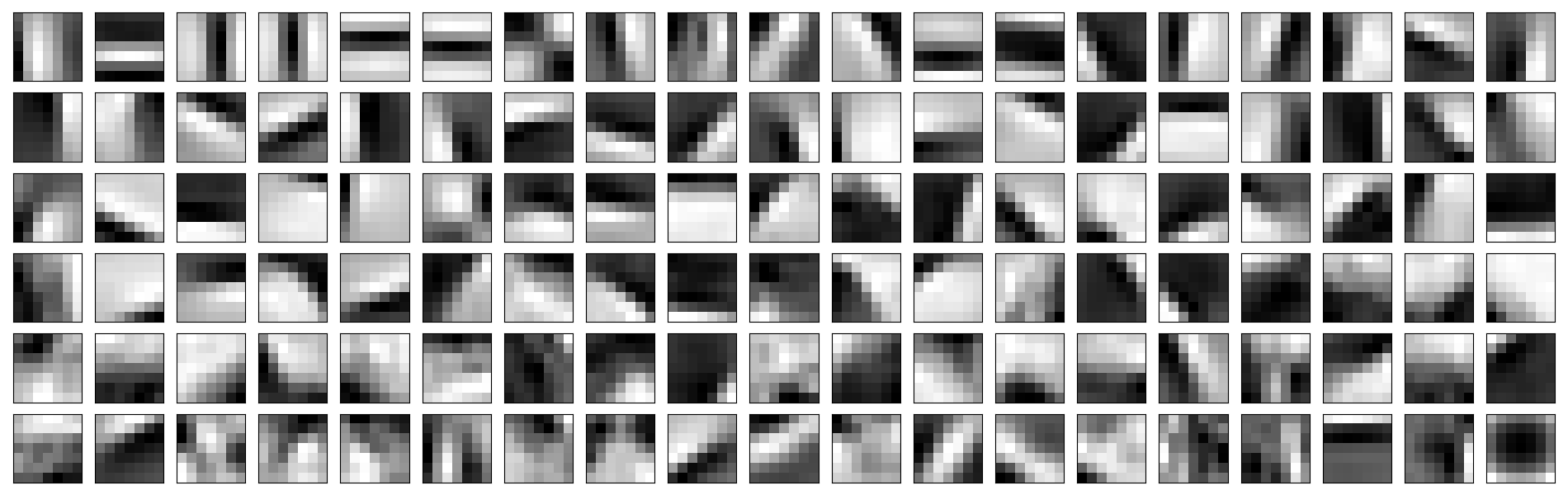
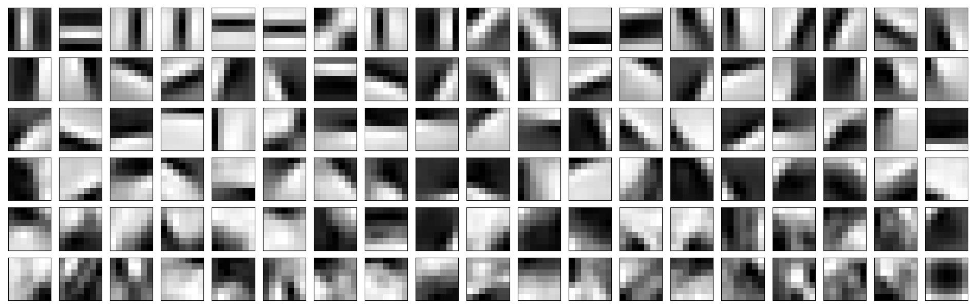
Figure 5: We divide the $7\times 7$ images in half to give two datasets, each with $400000=\frac{1}{2}(16\times 50000)$ datapoints of dimension $49$, keeping the number of images from each class roughly the same between the two halves. We apply Algorithm 1 to the two datasets and assess the similarity of the output. We obtain two matrices $A\in\mathbb{R}^{49\times J}$, where $J$ is the number of sources. We illustrate the results for $J=114$. The columns of the two $49\times 114$ matrices are plotted as grayscale $7\times 7$ images. We observe the visual agreement of the $114$ images, reflecting the identifiability. The last image is the Gaussian source, the Gaussian noise in the images. The two Gaussian sources have cosine similarity $0.99$. Their grayscale plots show that pixels patterns have more Gaussian noise at the center than the edges.

7.3 Protein data

We fit an adapted LiNGAM model [SHH⁺06] to a single-cell flow cytometry dataset [SPP⁺05]. Each datapoint measures 11 proteins in a cell. Suppose that the 11 proteins are $X_{1},\ldots,X_{11}$ and that $G$ is a directed acyclic graph with nodes $X_{1},\ldots,X_{11}$ whose edges $E(G)$ indicates causal relationships with weights $\lambda_{ij}$ on the edge $j\to i$. A linear structural equation model writes

$$X_{i}=\sum_{(j\to i)\in E(G)}\lambda_{ij}X_{j}+e_{i}.$$

The LiNGAM algorithm learns the graph $G$ from the higher-order cumulants of $X$, assuming the noise terms $e_{i}$ are non-Gaussian, using ICA. We use our algorithm for ICA with a Gaussian source to adapt the LiNGAM to allow a latent source of Gaussian noise:

$$X_{i}=\sum_{(j\to i)\in E(G)}\lambda_{ij}X_{j}+e_{i}+t_{i}y,$$

where $y$ is a Gaussian variable and $t_{i}$ is its effect on variable $X_{i}$. Let $\Lambda\in\mathbb{R}^{11\times 11}$ be the matrix of weights, with $(i,j)$ entry $\lambda_{ij}$. Then

$$\mathbf{X}=\Lambda\mathbf{X}+\mathbf{e}+\mathbf{t}y\quad\implies\quad\mathbf{X}=(I-\Lambda)^{-1}\mathbf{e}+(I-\Lambda)^{-1}\mathbf{t}y=((I-\Lambda)^{-1}|(I-\Lambda)^{-1}\mathbf{t})\begin{pmatrix}\mathbf{e}\\ y\end{pmatrix}.$$

Algorithm 1 recovers $A\in\mathbb{R}^{11\times 12}$ with first $11$ columns $(I-\Lambda)^{-1}$ and last column $(I-\Lambda)^{-1}\mathbf{t}$. As in the LiNGAM algorithm, this enables us to recover the directed acyclic graph $G$. But we also recover the vector $\mathbf{t}$, which measures the Gaussian noise effect for each $X_{i}$.

There are samples collected under 13 different perturbations in [SPP⁺05]. To test our adapted LiNGAM model via Algorithm 1, we divide the data from each perturbation into half to form two datasets. We log transform the data. We run our algorithm on each half of the data and compute the similarity of the Gaussian source effects, using cosine similarity, see Figure 6. We plot the Gaussian source effects in Figure 7.

Figure 6: For 1000 experiments, we plot a histogram of the cosine similarity of the Gaussian column of the mixing matrices (left). For comparison, we show the plot for two random matrices (right). Randomness comes from both tensor decomposition and the optimization step. The plot validates the choice of our adapted LiNGAM model, since the Gaussian source effects are consistent between experiments.

Figure 7: We fit our adapted LiNGAM model and focus on how the Gaussian source effects each protein. We plot the number of times each protein appears among the three entries of $\mathbf{t}$ with largest absolute value, across 100 repeats. It indicates that the (log-transformed) measurements of praf and pmek contain more Gaussian noise than the other proteins.

8 Conclusion

In this paper, we characterized the identifiability of overcomplete ICA. For generic mixing, we saw how identifiability is determined by the number of sources and the number of observations. We gave an algorithm for recovering the mixing matrix from the second and fourth cumulants and tested it on real and simulated data. Our algorithm allows for a Gaussian source, which is not true of other algorithms for ICA or overcomplete ICA.

We conclude by mentioning directions for future study.

• Theorem 1.9 gives three possibilities for generic identifiability: the middle case has a positive probability of identifiability and of non-identifiability. Compute these probabilities for a suitable distribution of mixing matrices.

• Adapt Theorem 1.9 and Algorithm 1 to incorporate structure on $A$, such as sparsity.

• Extend the complex identifiability results such as Theorem 6.1to the real setting.

• Study the special loci of identifiable and non-identifiable matrices geometrically, e.g. compute the dimension and degree of their Zariski closures.

Acknowledgements. We thank Chiara Meroni, Kristian Ranestad and Piotr Zwiernik for helpful discussions. AS was supported by the NSF (DMR-2011754). AS would like to thank the Isaac Newton Institute for Mathematical Sciences, Cambridge, for support and hospitality during the programme ‘New equivariant methods in algebraic and differential geometry’ where work on this paper was undertaken. This work was supported by EPSRC grant no EP/R014604/1.

References

- [ACCF04] Laurent Albera, Pierre Comon, Pascal Chevalier, and Anne Ferréol. Blind identification of underdetermined mixtures based on the hexacovariance. In 2004 IEEE International Conference on Acoustics, Speech, and Signal Processing, volume 2, pages ii–29. IEEE, 2004.
- [BKT08] Andrew Bashelor, Amy Ksir, and Will Traves. Enumerative algebraic geometry of conics. The American Mathematical Monthly, 115(8):701–728, 2008.
- [BMS02] Marian Stewart Bartlett, Javier R Movellan, and Terrence J Sejnowski. Face recognition by independent component analysis. IEEE Transactions on neural networks, 13(6):1450–1464, 2002.
- [CC02] Luca Chiantini and Ciro Ciliberto. Weakly defective varieties. Transactions of the American Mathematical Society, 354(1):151–178, 2002.
- [CJ10] Pierre Comon and Christian Jutten. Handbook of Blind Source Separation: Independent component analysis and applications. Academic press, 2010.
- [Com94] Pierre Comon. Independent component analysis, a new concept? Signal processing, 36(3):287–314, 1994.
- [COV17] Luca Chiantini, Giorgio Ottaviani, and Nick Vannieuwenhoven. On generic identifiability of symmetric tensors of subgeneric rank. Transactions of the American Mathematical Society, 369(6):4021–4042, 2017.
- [CS93] Jean-François Cardoso and Antoine Souloumiac. Blind beamforming for non-Gaussian signals. IEE proceedings F (radar and signal processing), 140(6):362–370, 1993.
- [Dar53] George Darmois. Analyse générale des liaisons stochastiques: etude particulière de l’analyse factorielle linéaire. Revue de l’Institut international de statistique, pages 2–8, 1953.
- [DLCC07] Lieven De Lathauwer, Josphine Castaing, and Jean-Franois Cardoso. Fourth-order cumulant-based blind identification of underdetermined mixtures. IEEE Transactions on Signal Processing, 55(6):2965–2973, 2007.
- [DLDMV01] Lieven De Lathauwer, Bart De Moor, and Joos Vandewalle. Independent component analysis and (simultaneous) third-order tensor diagonalization. IEEE Transactions on Signal Processing, 49(10):2262–2271, 2001.
- [DM04] Mike Davies and Nikolaos Mitianoudis. Simple mixture model for sparse overcomplete ICA. IEE Proceedings-Vision, Image and Signal Processing, 151(1):35–43, 2004.
- [EK04] J. Eriksson and V. Koivunen. Identifiability, separability, and uniqueness of linear ICA models. IEEE Signal Processing Letters, 11(7):601–604, 2004.
- [FMS20] Claudia Fevola, Yelena Mandelshtam, and Bernd Sturmfels. Pencils of quadrics: old and new. arXiv preprint arXiv:2009.04334, 2020.
- [GS02] Daniel R Grayson and Michael E Stillman. Macaulay2, a software system for research in algebraic geometry, 2002.
- [Har92] J. Harris. Algebraic Geometry: A First Course. Graduate Texts in Mathematics. Springer, 1992.
- [Har13] Robin Hartshorne. Algebraic geometry, volume 52. Springer Science & Business Media, 2013.
- [HCO99] Aapo Hyvarinen, Razvan Cristescu, and Erkki Oja. A fast algorithm for estimating overcomplete ICA bases for image windows. In IJCNN’99. International Joint Conference on Neural Networks. Proceedings (Cat. No. 99CH36339), volume 2, pages 894–899. IEEE, 1999.
- [Hea21] Thomas Little Heath. A history of Greek mathematics, Vol. 1: From Thales to Euclid. Clarendon Press, 1921.
- [JA95] A. Hirschowitz J. Alexander. Polynomial interpolation in several variables. J. Algebraic Geom. 4(4) (1995), 1995.
- [JK04] Christian Jutten and Juha Karhunen. Advances in blind source separation (BSS) and independent component analysis (ICA) for nonlinear mixtures. International journal of neural systems, 14(05):267–292, 2004.
- [JMM+01] T-P Jung, Scott Makeig, Martin J McKeown, Anthony J Bell, T-W Lee, and Terrence J Sejnowski. Imaging brain dynamics using independent component analysis. Proceedings of the IEEE, 89(7):1107–1122, 2001.
- [KLR73] A.M. Kagan, I.U.V. Linnik, and C.R. Rao. Characterization Problems in Mathematical Statistics. A Wiley-Interscience publication. Wiley, 1973.
- [KNH14] Alex Krizhevsky, Vinod Nair, and Geoffrey Hinton. The CIFAR- 10 dataset. University of Toronto, 2014.
- [KP19] Joe Kileel and Joao M Pereira. Subspace power method for symmetric tensor decomposition and generalized PCA. arXiv preprint arXiv:1912.04007, 2019.
- [Kru77] Joseph B. Kruskal. Three-way arrays: rank and uniqueness of trilinear decompositions, with application to arithmetic complexity and statistics. Linear Algebra and its Applications, 18(2):95–138, 1977.
- [LS00] Michael S Lewicki and Terrence J Sejnowski. Learning overcomplete representations. Neural computation, 12(2):337–365, 2000.
- [McC18] Peter McCullagh. Tensor methods in statistics. Courier Dover Publications, 2018.
- [Mor01] Eric Moreau. A generalization of joint-diagonalization criteria for source separation. IEEE Transactions on Signal Processing, 49(3):530–541, 2001.
- [Mum99] David Mumford. The red book of varieties and schemes: includes the Michigan lectures (1974) on curves and their Jacobians, volume 1358. Springer Science & Business Media, 1999.
- [OF+95] Bruno A Olshausen, David J Field, et al. Sparse coding of natural images produces localized, oriented, bandpass receptive fields. Submitted to Nature. Available electronically as ftp://redwood. psych. cornell. edu/pub/papers/sparse-coding. ps, 1995.
- [OSG20] Boris Odehnal, Hellmuth Stachel, and Georg Glaeser. The universe of quadrics. Springer Nature, 2020.
- [Pow64] Michael JD Powell. An efficient method for finding the minimum of a function of several variables without calculating derivatives. The computer journal, 7(2):155–162, 1964.
- [PPW+19] Anastasia Podosinnikova, Amelia Perry, Alexander S Wein, Francis Bach, Alexandre d’Aspremont, and David Sontag. Overcomplete independent component analysis via SDP. In The 22nd International Conference on Artificial Intelligence and Statistics, pages 2583–2592. PMLR, 2019.
- [SHH+06] Shohei Shimizu, Patrik O Hoyer, Aapo Hyvärinen, Antti Kerminen, and Michael Jordan. A linear non-Gaussian acyclic model for causal discovery. Journal of Machine Learning Research, 7(10), 2006.
- [SHMF14] Alexander Sokol, Marloes H. Maathuis, and Benjamin Falkeborg. Quantifying identifiability in independent component analysis. 2014.
- [Ski53] Viktor P Skitovitch. On a property of the normal distribution. DAN SSSR, 89:217–219, 1953.
- [Ski62] VP Skitovič. Linear combinations of independent random variables and the normal distribution law. 1962.
- [SPP+05] Karen Sachs, Omar Perez, Dana Pe’er, Douglas A Lauffenburger, and Garry P Nolan. Causal protein-signaling networks derived from multiparameter single-cell data. Science, 308(5721):523–529, 2005.
- [TLP04] Fabian J Theis, Elmar W Lang, and Carlos G Puntonet. A geometric algorithm for overcomplete linear ICA. Neurocomputing, 56:381–398, 2004.
- [UAIN15] Zahoor Uddin, Ayaz Ahmad, Muhammad Iqbal, and Muhammad Naeem. Applications of independent component analysis in wireless communication systems. Wireless personal communications, 83:2711–2737, 2015.