Mitigating Feature Gap for Adversarial Robustness
by Feature Disentanglement

Abstract

Deep neural networks are vulnerable to adversarial samples. Adversarial fine-tuning methods aim to enhance adversarial robustness through fine-tuning the naturally pre-trained model in an adversarial training manner. However, we identify that some latent features of adversarial samples are confused by adversarial perturbation and lead to an unexpectedly increasing gap between features in the last hidden layer of natural and adversarial samples. To address this issue, we propose a disentanglement-based approach to explicitly model and further remove the latent features that cause the feature gap. Specifically, we introduce a feature disentangler to separate out the latent features from the features of the adversarial samples, thereby boosting robustness by eliminating the latent features. Besides, we align features in the pre-trained model with features of adversarial samples in the fine-tuned model, to further benefit from the features from natural samples without confusion. Empirical evaluations on three benchmark datasets demonstrate that our approach surpasses existing adversarial fine-tuning methods and adversarial training baselines.

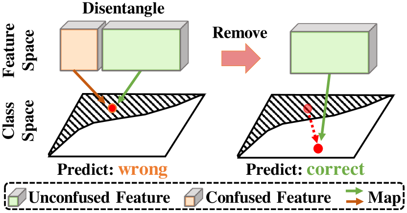
Figure 1: Toy illustration of Disentanglement. We model features of adversarial samples and then remove the latent features confused by adversarial perturbation to correct the prediction.

1 Introduction

Deep neural networks (DNNs) have shown impressive performances in various domains of machine learning. However, it has been demonstrated that DNNs are susceptible to adversarial samples and the prediction can be easily manipulated (Goodfellow et al., 2014). Adversarial samples deceive DNNs by introducing imperceptible noise to clean samples. With the widespread use of DNNs, the presence of adversarial samples poses a growing potential threat, making it crucial to enhance the robustness of networks.

Many defensive techniques are proposed including adversarial training (AT) (Madry et al., 2017; Zhang et al., 2019; Wang et al., 2020; Wu et al., 2020; Huang et al., 2020; Dong et al., 2021; Jia et al., 2022; Jin et al., 2022; Zhou et al., 2022), adversarial fine-tuning (AFT) (Suzuki et al., 2023; Maini et al., 2020; Madaan et al., 2021; Croce & Hein, 2022; Jeddi et al., 2020; Zhu et al., 2023; Si et al., 2020; Agarwal et al., 2023; Liu et al., 2023), adversarial purification (Yoon et al., 2021; Sun et al., 2023; Lee & Kim, 2023; Allen-Zhu & Li, 2022; Nie et al., 2022), adversarial detection (Hickling et al., 2023; Zheng & Hong, 2018; Pang et al., 2018), etc. It is universally acknowledged that AT is the most effective defensive technique, but it suffers from several times the training cost as standard (natural) training. To save the cost of training time, AFT employs the same loss function as AT to fine-tune the pre-trained model within a few epochs.

We identify an issue of the increasing feature gap by analyzing three models fine-tuned by three AFT methods (vanilla AFT, AFT+RGKD, ARREST) (Suzuki et al., 2023; Jeddi et al., 2020). As illustrated in Figure 2, the feature distance between natural and adversarial samples abnormally maintains an increasing direction during the fine-tuning process. Though ARREST initially exhibits notable fluctuations with a decreasing trend, the overall magnitudes of feature distance in three AFT methods show an increasing trend. We suppose that some latent features are easy to be confused by adversarial attacks and lead to the growing gap between the features of natural and adversarial samples. Considering that a robust model should treat natural and adversarial samples equally and extract similar features from them, we expect to remove the latent features causing the feature gap to achieve better robust performance.

In this paper, we analyze the latent features causing the feature gap and introduce an approach based on disentanglement to explicitly model and remove these features. We propose a new technique named Adversarial Fine-tuning via Disentanglement (AFD). First, we disentangle the features of adversarial samples as two components, in which the latent features causing the feature gap are identified as the features confused by adversarial perturbation. Next, we propose a feature disentangler to model and separate them from the features of adversarial samples. We maximize the predicted probabilities of the wrong predicted classes to acquire the latent features. Then we impose a constraint to distance the features of adversarial samples from them, to eliminate the latent features and mitigate the feature gap. Besides, we align features of adversarial samples in the fine-tuned model with features of natural samples in the naturally pre-trained model, further eliminating the latent features. Experiments demonstrate that our AFD alleviates the gap between features of natural and adversarial samples and improves the robustness. The key contributions are summarized as follows:

• We observe the gap in features between natural and adversarial samples anomalously increases when applying adversarial fine-tuning methods, resulting from the latent features confused by adversarial perturbation.

• We propose a disentanglement-based approach, which explicitly models and further eliminates the latent features causing the feature gap by a disentangler and loss function of alignment.

• Empirical evaluations show our approach mitigates the gap in features between natural and adversarial samples and surpasses existing methods. We also provide extended analyses for a holistic understanding.

2 Related Work

Adversarial Training Adversarial training (AT) is the most effective technique to defend against attacks. Numerous studies have been conducted to boost robustness and improve the trade-off between accuracy and robustness. Madry et al. (2017) propose Projected Gradient Descent (PGD) attack and PGD-based adversarial training (PGD-AT), compelling the model to correctly classify adversarial samples within the epsilon sphere during training, which is the pioneer in adversarial learning. Zhang et al. (2019) reduce the divergence of probability distributions of natural and adversarial samples to mitigate the difference between robust and natural accuracy. Wang et al. (2020) find that misclassified samples harm adversarial robustness significantly, and propose to improve the model’s attention to misclassification by adaptive weights. Huang et al. (2020) replace labels with soft labels predicted by the model and adaptively reduce the weights of misclassified samples to alleviate the robust overfitting problem. Dong et al. (2021) also propose a similar idea of softening labels and explain the different effects of hard and soft labels on robustness by investigating the memory behavior of the model for random noisy labels. Zhou et al. (2022) embed a label transition matrix into models to infer natural labels from adversarial noise. Though AT has good robust performances, it suffers from a large quantity of computing expenses and training costs. Some researchers have developed approaches to accelerate adversarial training, commonly known as fast adversarial training (FAT) (Wong et al., 2020; Kim et al., 2020; Huang et al., 2023). Since these FAT methods only require a little training time like AFT, we compare them with our method.

Adversarial Fine-tuning Adversarial fine-tuning (AFT) has been employed to enhance the pre-trained model within a few epochs for various targets, particularly for achieving adversarial robustness. Moosavi-Dezfooli et al. (2018) analyze the effect of AFT by comparing the decision boundary of a DNN before and after applying AFT. Some researchers (Tramer & Boneh, 2019; Maini et al., 2020; Madaan et al., 2021; Croce & Hein, 2022) aim to achieve multiple $l_{p}$ adversarial robustness through specific strategies. Jeddi et al. (2020) employ vanilla AFT to expedite the training of robust models with a few training epochs and a warm-up learning rate schedule. Based on representation learning, Suzuki et al. (2023) propose ARREST and AFT+RGKD, which reduce the feature gap between natural and adversarial samples. Zhu et al. (2023) propose a metric to measure the robustness of modules and fine-tune them for better out-of-distribution performance. Liu et al. (2023) introduce a two-pipeline structure to improve the relationship between the weight norm and its gradient norm in batch normalization layers. Despite the extensive work, few methods (vanilla AFT, ARREST, and AFT+RGKD) are based on naturally pre-trained models, which are important baselines in our paper.

3 Methodology

In this section, we first reveal the issue of the increasing gap of features between natural and adversarial samples in AFT. Then we introduce a disentanglement-based method, to model and further remove the latent features leading to the feature gap. Our method is expected to mitigate the feature gap to enhance adversarial robustness.

3.1 Preliminaries

We denote a DNN as $h(x)=\omega\cdot g(x;\theta_{g})$, where $x$ is the input image, and $\theta_{g}$ is the parameters of the feature extractor $g$, i.e., the model before the last linear classifier. $\omega$ denotes the parameters of the last linear classifier. The parameters of the naturally pre-trained and fine-tuned model are denoted as $\theta^{P}$ and $\theta^{F}$, respectively. The architecture and dataset for both pre-training and fine-tuning remain consistent, and the model parameters $\theta^{F}$ are initialized by $\theta^{P}$. $x$ denotes the clean sample, and $x^{\prime}$ denotes the adversarial sample. ${\|{\delta}\|}_{p}\leq\epsilon$ denotes the adversarial perturbation, where $\epsilon$ represents the budget of adversarial attack. We use ${\|{\cdot}\|}_{p}$ to denote the $l_{p}$ norm. Adversarial and natural features denote the features in the last hidden layer of adversarial and natural samples, i.e., $g(x^{\prime};\theta_{g})$ and $g(x;\theta_{g})$ respectively. $\mathcal{L}$ denotes the cross-entropy loss.

3.2 Model the Latent Feature causing Feature Gap

We evaluate the feature gap in AFT by measuring the ${L}_{p}$ distance between natural and adversarial features. As shown in Figure 2, the overall magnitudes of feature distance between natural and adversarial samples in three AFT methods (vanilla AFT, ARREST, AFT+RGKD) are becoming larger. The gap between the two types of features in ARREST initially decreases and then increases, which exhibits a V-shape trend. In addition, the feature gap in other AFT methods presents a consistently increasing trend. Despite AFT enhancing robust accuracy during training, the feature distance in AFT maintains a growing trend overall. Intuitively, the ideal robust model should have a consistent understanding and analysis of natural and adversarial samples, thus extracting similar (the same) features from them. Figure 2 indicates that existing AFT methods neglect the gap of features between natural and adversarial samples. Narrowing the feature gap is expected to achieve better performance and enhance robust accuracy.

To realize the target, we can disentangle two types of features from the features of natural and adversarial samples. We define natural features $f_{nat}$ as the unconfused features $f_{u}$. We can define adversarial features $f_{adv}$ as the combination of the unconfused features $f_{u}$ and the confused features $f_{c}$, the latter of which leads to the gap in features between natural and adversarial samples. In this modeling, the unconfused features represent the features that contribute to accurate classification, which are easily extracted from natural samples. Besides, the confused features are identified as the latent features causing the gap between features of natural and adversarial samples, which are confused by the adversarial perturbation. As illustrated in Figure 1, if the confused features are removed in adversarial features, the features of adversarial samples can align with those of natural samples, resulting in a zero feature gap and accurate predictions for adversarial samples.

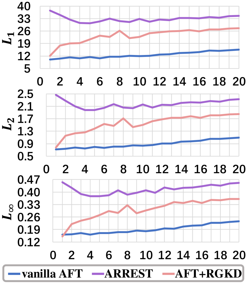
Figure 2: $L_{p}$ distances of features between natural and adversarial samples on ResNet18 on CIFAR-10. The horizontal axis denotes the training epoch. Despite the initial decreasing fluctuations observed in ARREST and AFT+RGKD, AFT methods exhibit an increasing trend on the whole.

We suppose the phenomenon in Figure 2 is attributable to the presence of the confused features $f_{c}$. Because the confused features persist as latent features and don’t diminish during fine-tuning, the gap between features of natural and adversarial samples cannot be bridged. The confused features induce the gap between natural and adversarial features, leading to the limited robust performance. Based on our observations and analyses, we introduce a new approach named Adversarial Fine-tuning via Disentanglement (AFD), as shown in Figure 3. It applies a feature disentangler to explicitly extract the confused features, and remove them by the elimination and alignment of features.

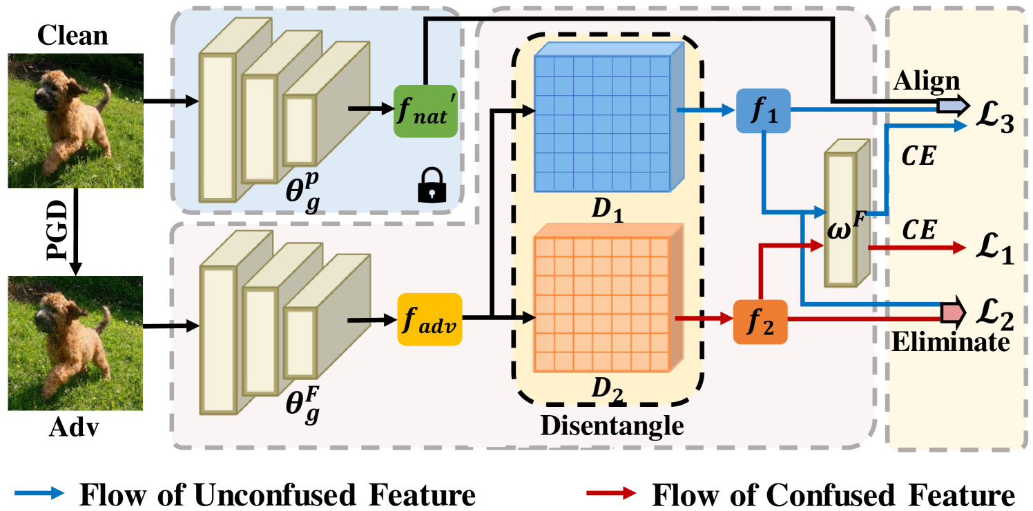
Figure 3: Overview of our AFD. Lock denotes the frozen parameters. The disentangler disentangles adversarial features into $f_{1}$ and $f_{2}$. We obtain confused features $f_{2}$ by matching the wrong predicted labels in $\mathcal{L}_{1}$. Next, we employ $\mathcal{L}_{2}$ to eliminate confused features from unconfused features $f_{1}$. Besides, we apply $\mathcal{L}_{3}$ to further align $f_{1}$ with pre-trained unconfused features $f_{nat}^{\prime}$ to correct the prediction.

3.3 Adversarial Fine-tuning Based on Disentanglement

The primary strategy is to explicitly disentangle the unconfused and confused features from the features of adversarial samples. We propose a feature disentangler to model confused features for further elimination. The features in the last hidden layer are input into the disentangler, yielding two disentangled feature vectors. We define these feature vectors as 1) $f_{1}$, features contributing to correct classification without confusion; and 2) $f_{2}$, features inducing wrong predictions of adversarial samples. To implement this disentangling, we introduce a disentangler with two linear blocks $D_{1},D_{2}$ between the feature extractor $g$ and the linear classifier $\omega$. These linear blocks are expected to disentangle adversarial features into the unconfused features and confused features. The disentangled feature vectors $f_{1}$ and $f_{2}$ are constrained to match the unconfused features and confused features, formulated as:

$$\begin{split}f_{1}&=\ {D_{1}}(g(x^{\prime};\theta_{g}^{F});\theta_{D_{1}}),\\ f_{2}&=\ {D_{2}}(g(x^{\prime};\theta_{g}^{F});\theta_{D_{2}}),\\ {\rm where}\ &\left\{\begin{array}[]{lr}f_{1}\stackrel{{\scriptstyle D_{1}}}{{\longrightarrow}}f_{u},&\\ f_{2}\stackrel{{\scriptstyle D_{2}}}{{\longrightarrow}}f_{c},&\end{array}\right.\end{split}$$ (1)

where $\theta_{g}^{F}$ denotes the parameters of the feature extractor in the fine-tuned model. We take $f_{1}$ to correctly classify samples and $f_{2}$ to match the confused features. The input and output dimensions of the linear block $D_{1},D_{2}$ are set to match the channel dimensions of the feature vector of adversarial samples before disentanglement. This ensures the parameters of the linear block $\theta_{D_{1}}$ can be seamlessly integrated with the parameter of the last linear classifier $\omega^{F}$, expressed as $\theta_{D_{1}}\cdot\omega^{F}={\omega^{F\prime}}$. Thus we only need to load the linear classifier $\omega^{F\prime}$ without additional disentangling modules in the deployment (test) phase.

To achieve good performance on both accuracy and robustness, we should design suitable loss functions to realize Formula 1. First, we suggest fitting $f_{2}$ to incorrectly predicted labels $y^{\prime}$ to model the confused features. The confused features result in obvious shifts in both features and predicted probabilities, leading to wrong predicted class labels in most cases. Thus, it can be identified as the latent features causing the gap between natural and adversarial features. To disentangle the confused features from adversarial features, we force the disentangled features $f_{2}$ to match incorrect class labels, formulated as:

$$\begin{split}\mathcal{L}_{1}=\ &{\rm\mathop{arg\ min}\limits_{\theta_{D_{2}}}}\ \mathcal{L}(\omega^{F}\cdot f_{2},y^{\prime}),\\ {\rm where}\quad&y^{\prime}={\rm\mathop{arg\ sort}\limits_{y^{\prime}\neq y}}\ \omega^{F}\cdot f_{1},\end{split}$$ (2)

where $y^{\prime}$ denotes wrong predicted labels with the maximum predicted probability, and sort represents finding the index of the maximum value. We only optimize the disentangling block $D_{2}$ instead of the entire model. This selective optimization prevents potential harm to the feature extractor that could result from learning the confused features.

In addition, we introduce a constraint on $f_{1}$ to keep away from the confused features $f_{2}$, removing the confused features from the features of adversarial samples. The exclusive force between $f_{1}$ and $f_{2}$ encourages the elimination of the confused features from the features of adversarial samples. This constraint aims to protect adversarial features from being perturbed by the confused features, and then gain the unconfused features $f_{1}$. Given by:

$$\mathcal{L}_{2}={\rm\mathop{arg\ max}\limits_{\theta^{F},\theta_{D_{1}}}}\ \mathcal{D}(f_{1},\bar{f_{2}}),$$ (3)

where $\mathcal{D}$ denotes a distance function, $\bar{f_{2}}$ means the gradient back-propagation of $f_{2}$ is frozen.

3.4 Adversarial Fine-tuning Based on Alignment

The second strategy is to align the adversarial features in the fine-tuned model with the natural features in the pre-trained model. Since the pre-trained model has a high natural accuracy and doesn’t suffer from adversarial attacks, the natural features in the pre-trained model can be identified as ideal unconfused features. Thus, adversarial features in the fine-tuned model can be greatly improved by being aligned with the natural features in the pre-trained model. Besides, lots of work (Zhang et al., 2019; Wang et al., 2020; Suzuki et al., 2023) conducts an alignment between natural and adversarial features, which is regarded to mitigate the trade-off between accuracy and robustness. We take the disentangled features $f_{1}$ to match the natural features in the pre-trained model, further removing the confused features from $f_{1}$. The AFT loss function with the alignment can be formulated as:

$$\mathcal{L}_{3}={\rm\mathop{arg\ min}\limits_{\theta^{F},\theta_{D_{1}}}}\ \mathcal{L}(\omega^{F}\cdot f_{1},y)+\gamma\cdot\mathcal{D}(f_{1},g(x;\theta_{g}^{P})),$$ (4)

where $\theta_{g}^{P}$ denotes parameters of the feature extractor in the pre-trained model, and $\gamma$ denotes the weight of the alignment. Therefore, the objective function of our AFD is defined as follows:

$$\mathcal{L}_{total}=\alpha\cdot\mathcal{L}_{1}+\beta\cdot\mathcal{L}_{2}+\mathcal{L}_{3},$$ (5)

where $\alpha$ and $\beta$ denote the weights of $\mathcal{L}_{1}$ and $\mathcal{L}_{2}$. The algorithm of AFD is as follows:

Algorithm 1 Adversarial Fine-tuning via Disentanglement

0:  Training set $\mathcal{D}$, The $\mathcal{L}_{1}$ weight $\alpha$, The $\mathcal{L}_{2}$ weight $\beta$, Number of epochs $T$, Learning rate $\eta$, Inner maximization $\mathcal{A}$, Naturally pre-trained model parameters $\theta^{P}$, Model parameters except linear block $D_{2}$ parameters $\theta_{1}$, Linear block $D_{2}$ parameters $\theta_{2}$.

0:  Fine-tuned model parameters $\theta_{1}$.

  Initialize $\theta_{1}$ by $\theta^{P}$;

  for $t=1,\cdots,T$ do

     for $x,y\in\mathcal{D}$ do

        $x^{\prime}=\mathcal{A}(x)$;

        Calculate features $f_{1},f_{2}$ by Formula 1;

        Calculate loss $\mathcal{L}_{1}$ by Formula 2;

        $\theta_{2}=\theta_{2}-\eta\cdot\frac{\mathrm{d}(\alpha\cdot\mathcal{L}_{1})}{\mathrm{d}\theta_{2}}$;

        Calculate loss $\mathcal{L}_{2}$ by Formula 3;

        $\theta_{1}=\theta_{1}-\eta\cdot\frac{\mathrm{d}(\beta\cdot\mathcal{L}_{2})}{\mathrm{d}\theta_{1}}$;

        Calculate loss $\mathcal{L}_{3}$ by Formula 4;

        $\theta_{1}=\theta_{1}-\eta\cdot\frac{\mathrm{d}\mathcal{L}_{3}}{\mathrm{d}\theta_{1}}$;

     end for

  end for

4 Experiments

This section presents experiments with AFD. We first introduce our experiment setting. We further make comparisons on multiple architectures and datasets to show our superiority. Then we conduct an ablation study to show the functions of the disentangling module and alignment. Finally, we conduct an empirical analysis to support our hypothesis.

4.1 Setting

Datasets We conduct our experiments on three benchmark datasets including on CIFAR-10 and CIFAR-100 (Krizhevsky, 2009), Tiny-ImageNet (Deng et al., 2009). CIFAR-10 dataset contains 60,000 color images having a size of $32\times 32$ in 10 classes, with 50,000 training and 10,000 test images. CIFAR-100 dataset contains 50,000 training and 10,000 test images in 100 classes. Tiny-ImageNet dataset contains 100000 images of 200 classes (500 for each class) downsized to 64×64 colored images. Each class has 500 training images, 50 validation images and 50 test images. We only use training and validation images of Tiny-ImageNet in experiments.

Baselines To make a comprehensive comparison, we have employed various techniques to demonstrate our superiority. Our primary baselines are AFT methods including vanilla AFT (vAFT) (Jeddi et al., 2020), AFT+RGKD (AFKD) (Suzuki et al., 2023), and ARREST (Suzuki et al., 2023). All of them are built upon naturally pre-trained models. Additionally, we compare our AFD with state-of-the-art AFT methods such as RiFT (Zhu et al., 2023) and TWINS (Liu et al., 2023), which rely on adversarially pre-trained models. Besides, we select several advanced fast adversarial training methods for comparison, including FreeAT (Shafahi et al., 2019), FGSM-GA (Andriushchenko & Flammarion, 2020), ATAS (Huang et al., 2023), since they are also low-cost techniques. Moreover, we compare with baseline methods of adversarial training including PGD-AT (Madry et al., 2017), TRADES (Zhang et al., 2019) to show our great advance in robustness.

Optimization Details The optimizer used in all the experiments is Stochastic Gradient Descent (SGD) optimizer with a momentum of 0.9. We naturally pre-train all the models with a batch size of 128, training epochs of 100, and a weight decay of ${5.0\times 10^{-4}}$. The learning rate starts at 0.1 and then decays by $\times$0.1 with transition epochs $\{75,90\}$, following Zhang et al. (2019). For AT methods, we train all the models with a batch size of 128, training epochs of 120, and a weight decay of ${2.0\times 10^{-4}}$. The learning rate starts at 0.1 and then decays by $\times$0.1 with transition epochs $\{75,90,100\}$, following Wang et al. (2020). For our AFD, we fine-tune the pre-trained models with a batch size of 128, an initial learning rate of 0.0025, a weight decay of ${5.0\times 10^{-4}}$, and training epochs of 20. The learning rate is changed to 0.0020 at the 11th epoch and is divided by half every two epochs thereafter, as Suzuki et al. (2023).

Implementation Details We use ResNet18 (He et al., 2016) and WideResNet-34-10 (Zagoruyko & Komodakis, 2016) as the main DNN architectures, following previous studies (Goldblum et al., 2020; Suzuki et al., 2023; Wang et al., 2020). In particular, we utilize ResNet50 (He et al., 2016) to fairly compare with TWINS. The distance function chosen for $\mathcal{L}_{2}$ and $\mathcal{L}_{3}$ is the angular distance: $\mathcal{D}(u,v)=1-\frac{u\cdot v}{{\|{u}\|}_{2}\cdot{\|{v}\|}_{2}}$. $L_{\infty}$-norm PGD (Madry et al., 2017) with a random start, a step size of 0.007, attack iterations of 10, and a perturbation budget of $8/255$ is used to solve the inner maximization of our AFD. After fine-tuning, we test the natural accuracy (Clean) and apply two white-box attacks for evaluation: PGD (Madry et al., 2017) and AutoAttack (AA) (Croce & Hein, 2020). The maximum perturbation used for evaluation is also set to $8/255$. $L_{\infty}$-norm PGD with a random start, a step size of 0.003, and attack iterations of 20 (PGD-20) is utilized in the evaluation. In the following tables, ${\dagger}$ denotes the results excerpted in the papers (Huang et al., 2023; Liu et al., 2023), which are evaluated by PGD-10 in the manuscript. Bold type indicates the highest value for each metric. We only report the results of the last epoch.

4.2 Main Results against White-Box Attack

To evaluate AFD’s effectiveness, we conducted comparative experiments with other methods on CIFAR-10, CIFAR-100, and Tiny-ImageNet. We also make additional experiments on ResNet50 to fairly compare with TWINS.

CIFAR-10 and CIFAR-100 As shown in Tables 1, methods above the double line denote AT and FAT methods, and methods under the double line denote AFT methods. It shows that among AFT methods, AFD exhibits the best robust performance and ARREST has the second best robust performance on ResNet18. Robust accuracies of AFD against AutoAttack (AA) surpass those of ARREST by 1.27% and 2.58% on CIFAR-10 and CIFAR-100, respectively. As indicated in Table 2, AFD exhibits the best robust performance and AFKT has the second best robust performance among all the methods on WideResNet-34-10. AFD achieves superior robust accuracies against AA compared to AFKD, with improvements of 2.05% and 2.34% on CIFAR-10 and CIFAR-100, respectively. In particular, RiFT doesn’t show great robust performances, since it is fine-tuned with natural data to enhance out-of-distribution performance.

Besides, AFD with fewer training epochs outperforms AT methods. AFD surpasses PGD-AT in all respects. TRADES achieves a larger robust accuracy against AA on CIFAR-10 on ResNet18 than AFD by 1.02%. However, the situation is reversed on CIFAR-100 or on WideResNet-34-10, where AFD outperform TRADES against AA by 0.43%, 2.40%, and 2.37%. This can be attribute to the superiority of AFD and the robust over-fitting in AT. Moreover, FAT methods distinctly lag behind AFD in both natural and robust performances. Despite the advanced robust performance of AFD, its natural accuracy doesn’t surpass state-of-the-art AFT methods (ARREST). We make further discussion in the Section 4.3. In summary, AFD demonstrates superb robustness compared to AT, FAT and AFT methods.

Table 1: Quantitative evaluations of AFD and other methods for CIFAR-10 and CIFAR-100 on ResNet18.

Methods	CIFAR-10			CIFAR-100
	Clean	PGD	AA	Clean	PGD	AA
PGD-AT	84.43	48.82	43.68	59.09	24.05	20.67
TRADES	82.37	53.27	48.52	55.47	28.12	23.49
Free-AT†	78.37	40.90	36.00	50.56	19.57	15.09
FGSM-GA†	80.10	49.14	43.44	50.61	24.48	19.42
ATAS†	81.22	50.03	45.38	55.49	27.68	22.62
vAFT	83.93	51.40	45.48	60.83	26.55	21.96
RiFT	84.49	49.24	43.66	59.51	24.01	20.48
AFKD	84.71	51.32	46.09	65.54	28.09	22.92
ARREST	85.71	51.23	46.23	67.00	26.89	21.34
AFD	84.66	52.63	47.50	62.94	29.27	23.92

Table 2: The performance of AFD and other methods on CIFAR-10 and CIFAR-100 on WideResNet-34-10.

Methods	CIFAR-10			CIFAR-100
	Clean	PGD	AA	Clean	PGD	AA
PGD-AT	86.35	49.57	45.81	60.30	25.14	22.65
TRADES	85.68	52.53	49.22	57.67	28.26	25.25
vAFT	87.42	53.57	48.49	64.92	27.19	23.59
RiFT	84.49	49.24	45.83	60.59	25.57	22.67
AFKD	88.54	54.86	49.57	68.50	30.12	25.28
ARREST	88.42	54.16	49.45	69.52	29.47	24.55
AFD	88.08	56.12	51.62	68.51	32.63	27.62

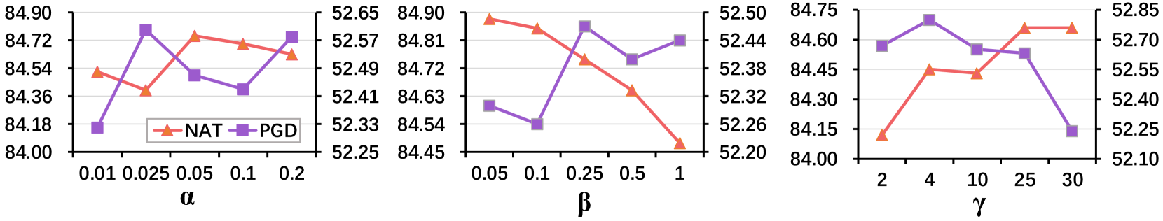
Figure 4: The clean accuracy (NAT) and robust accuracy against PGD-20 (PGD) of AFD with different hyperparameters.

Tiny-ImageNet We further conduct comparative experiments on a larger dataset, Tiny-ImageNet. As shown in Table 3, on ResNet18, AFD consistently outperforms all the methods in terms of robust performance and the robust performance of TRADES ranks second. The robust accuracy of AFD against PGD exceeds that of TRADES by 1.59% and its robust accuracy against AA outpaces that of TRADES by 1.58%. Moreover, on WideResNet-34-10, AFD keeps the best robust performance and AFKD exhibits the second best robust performance. The robust accuracy of AFD against PGD on WideResNet-34-10 surpasses that of AFKD by 2.56% and its robust accuracy against AA on WideResNet-34-10 is higher than that of AFKD by 2.76%. These findings indicate the superiority of AFD in terms of adversarial robustness on large datasets.

Table 3: The performances of AFD and other methods on Tiny-ImageNet with ResNet18 and WideResNet-34-10 models.

Methods	ResNet18			WideResNet-34-10
	Clean	PGD	AA	Clean	PGD	AA
PGD-AT	52.12	19.38	16.79	54.24	19.03	16.51
TRADES	49.28	22.59	17.06	49.22	23.33	18.51
vAFT	52.75	21.29	16.76	57.17	22.24	18.02
RiFT	52.24	20.89	17.05	55.09	19.51	16.79
AFKD	57.17	22.29	16.68	60.92	24.27	19.01
ARREST	60.36	19.28	12.58	65.07	22.73	16.67
AFD	55.58	24.18	18.64	59.58	26.83	21.77

ResNet50 We follow Liu et al. (2023) to make comparisons on ResNet50. Notice that TWINS employs a model adversarially pre-trained on ImageNet (Deng et al., 2009), and the number of its training periods is 60. We set the training epochs of AFD as 40. Results are shown in Table 4. Although TWINS benefits from prior knowledge of ImageNet and adversarial robustness of the pre-trained model, AFD still surpasses its robust performance on both CIFAR-10 and CIFAR-100. AFD achieves improvements of 1.54% and 1.56% under AA compared to TWINS, and its robust accuracies against PGD surpass those of TWINS by 1.88% and 2.52%. This demonstrates its superiority in terms of adversarial robustness on ResNet50.

Table 4: The performances of AFD and the state-of-the-art method TWINS on CIFAR-10 and CIFAR-100 on ResNet50.

Methods	CIFAR-10			CIFAR-100
	Clean	PGD	AA	Clean	PGD	AA
PGD-AT†	89.77	52.24	48.46	69.48	28.52	23.47
TWINS†	91.95	52.46	49.02	72.12	29.12	25.72
AFD	86.31	54.34	50.56	65.48	31.64	27.28

In summary, these experiments indicate that AFD always outperforms all the baselines for different adversarial attacks, datasets, and network architectures in the aspect of robustness.

4.3 Ablation Study

Effect of Disentangler As mentioned in Section 3.3, the disentangler should disentangles adversarial features into the confused and unconfused features, and further eliminate the confused features. As shown in Table 5, vAFT with the disentangler (vAFT+D) exhibits superior robustness compared to vAFT by 1.28% against PGD and by 1.40% against AA, respectively. It shows the feature disentangler effectively eliminates the confused features that lead to wrong predictions. Moreover, the natural accuracy of AFT-D outperforms that of AFT by 0.70%. This could be attributed to the disentangling module removing the class-irrelevant features of natural samples such as background and shadow.

Effect of Alignment As shown in Table 5, vAFT with the alignment of features (vAFT+A) exhibits superior robustness compared to AFT against both PGD and AA by 0.39% and 0.72%, with a marginal increase in natural accuracy by 0.67%. It indicates that the alignment successfully assists to further remove the confused features.

Effect of Combination The combination of disentangler and alignment (AFD) has the best performance on both natural and robust accuracy, which shows two strategies are compatible and the combination can boost the positive effects of individual strategies. However, in Table 1 and other tables, AFD exhibits a lower natural accuracy than state-of-the-art AFT methods. This is because the unconfused features $f_{1}$ have not been trained with natural samples, which may lead to an accuracy-robust trade-off.

Table 5: The performances of vAFT and other methods on CIFAR-10 on ResNet18. ‘+D’ denotes the method with the disentangler, and ‘+A’ denotes the method with the alignment of features.

Methods	vAFT	vAFT+D	vAFT+A	AFD
Clean	83.93	84.63	84.61	84.66
PGD	51.40	52.68	51.71	52.63
AA	45.48	46.88	46.81	47.50

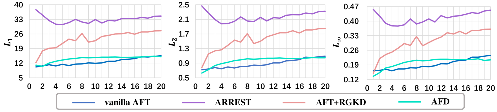
Figure 5: $L_{p}$ distances of features between natural and adversarial samples. The horizontal axis represents the training epoch.

Effect of Hyperparameter There are three hyperparameters in our AFD: $\alpha,\beta$ and $\gamma$. They control the weights of $\mathcal{L}_{1}$, $\mathcal{L}_{2}$, and the distance function in $\mathcal{L}_{3}$, respectively. We have conducted experiments with various combinations of weights on ResNet18 on CIFAR-10, as illustrated in Figure 4. There is a remarkable trade-off between accuracy and robustness when $\beta$ and $\gamma$ are growing. On the one hand, a larger value of $\beta$ indicates a larger exclusive force between the unconfused and confused features, leading to less non-robust features utilized in classification and better robustness. On the other hand, as $\gamma$ increases, the natural accuracy increases but robust accuracy drops. This occurs because more feature information of natural samples is transferred to the fine-tuned model through the feature alignment. However, the variations of both natural and robust accuracy are less than 0.60%, demonstrating that our AFD is insensitive to variations of hyperparameters.

4.4 Empirical Analysis of Disentangled Features

We evaluate the performances of two types of disentangled features $f_{1}$, $f_{2}$ on various datasets and models. As shown in Table 6, the natural accuracies of $f_{2}$ are lower than those of $f_{1}$ by $4.53\%\sim 45.05\%$. It indicates the disentangler has successfully extracted and removed the confused features as $f_{2}$. High accuracies of $f_{1}$ indicates models benefit from eliminating the confused features. Interestingly, the disparity of accuracy on CIFAR-100 is smaller than that on CIFAR-10. We suppose that a dataset with more classes has more complex feature space, and it is more difficult to extract confused features by the linear disentangler. Maybe nonlinear disentanglers work better.

Table 6: The natural accuracies of the unconfused features $f_{1}$ and confused features $f_{2}$. RN and WRN are abbreviations of ResNet and WideResNet, respectively. $\Delta$ denotes the accuracy disparity.

Model	Data	$f_{1}$	$f_{2}$	$\Delta$
RN18	CIFAR-10	84.66	39.61	45.05
RN18	CIFAR-100	62.94	58.41	4.53
RN50	CIFAR-10	83.18	47.35	35.83
RN50	CIFAR-100	61.68	54.97	6.71
WRN-34-10	CIFAR-10	88.08	46.89	41.19
WRN-34-10	CIFAR-100	68.51	62.84	5.67

Moreover, we analyze the feature distance between the unconfused features $f_{1}$ and natural features $f_{nat}$, as illustrated in Figure 5. In contrast to the growing trend of feature distance in existing AFT methods, the optimization trajectory of the feature distance in AFD exhibits a fast convergence trend. It implies that AFD has mitigated the gap between natural and adversarial features. Additionally, the magnitudes of the feature distance in AFD are smaller than other AFT methods, e.g., the $L_{\infty}$ distance of AFD (0.214) is notably less than those of ARREST and vanilla AFT (0.453, 0.236). These results demonstrates our disentanglement-based approach can enhance the adversarial robustness by alleviating the feature gap.

5 Conclusion

This paper uncovers a surprising increasing trend in the gap of features between natural and adversarial samples in AFT methods, and further investigates it from the perspective of features. We model features as two feature components, in which the confused features are defined as the latent features leading to the feature gap. Then we propose Adversarial Fine-tuning via Disentanglement (AFD) to bridge the feature gap to enhance robustness. Our approach contains two strategies: disentanglement and alignment. We design the feature disentangler to explicitly separate out the confused features from the features of adversarial samples, while the second strategy aligns the adversarial features with the natural features in the pre-trained model. Experiments demonstrate that AFD effectively mitigates the feature gap and achieves significant robust performance, even surpasses adversarial training methods. Future work will aim at the accuracy-robustness trade-off.

Appendix A Performances of Pre-trained models

Table 7: The natural accuracy of the naturally pre-trained models.

Model	Data	Clean
ResNet18	CIFAR-10	94.60
ResNet18	CIFAR-100	76.55
ResNet18	Tiny-ImageNet	64.81
ResNet50	CIFAR-10	94.30
ResNet50	CIFAR-100	77.20
WideResNet-34-10	CIFAR-10	95.53
WideResNet-34-10	CIFAR-100	80.28
WideResNet-34-10	Tiny-ImageNet	67.86

We conduct pre-training experiments on multiple datasets and architectures. As shown in Table 7, all of the pre-trained models have much higher accuracies than the fine-tuned models. It indicates that it is reasonable for feature alignment to regard features of the natural samples in the pre-trained models as the ideal unconfused features.

Appendix B Feature Visualization

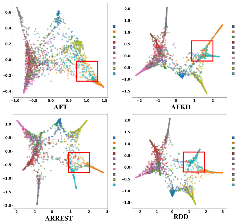
Figure 6: t-SNE visualization of different methods. The proposed AFD shows a clearer separation in the area of the red box.

To further demonstrate the effectiveness of AFD, Figure 6 visualizes the features of AFT methods using t-SNE (Van der Maaten & Hinton, 2008) on ResNet18 on CIFAR-10. We color each point to match its ground-truth label and highlight focused areas with red boxes. It shows the disentangled features learned by AFD have a much clearer class boundary than those learned with other methods. This indicates that AFD successfully mitigates the confusion between features of distinct classes, leading to a more robust prediction.

Appendix C Environments and Time of Experiments

Table 8: The training time (second) of various methods on ResNet18 on CIFAR10. We show the time for one epoch (${\rm Time_{one}}$) and the expected values of the total time (${\rm Time_{total}}$).

Method	Epoch	${\rm Time_{one}}$	${\rm Time_{total}}$
Standard	100	6.0	590
PGD-AT	120	37	4440
PGD-AT†	-	-	4428
TARDES	120	53	6360
Free-AT†	10	119	1188
FGSM-GA†	30	68	2052
ATAS†	30	36	1080
vanilla AFT	20	37	1330
RiFT	10	25	4690
AFKD	20	40	1390
ARREST	20	36	1310
AFD	20	46	1510

We have conducted experiments on a machine with three NVIDIA GeForce RTX 4090 GPUs. We use a single GPU for ResNet models and three GPUs for WideResNet models. We measure the training time as an evaluation indicator. ‘Standard’ denotes the time of natural pre-training. Though the results with ${\dagger}$ are evaluated on a different machine, their training time of PGD-AT is almost the same as ours. Thus we think it is fair to compare our training time with theirs.

As shown in Table 8, TRADES costs the most time and ATAS costs the least time among all the methods. The time cost of RiFT surpasses those of other AFT methods because it needs an adversarially pre-trained model. Our AFD costs less time than TRADES by 4850 seconds and its total training time outperforms that of vanilla AFT by 180 seconds. Considering its advanced robustness, the time cost is worthy and acceptable.

References

- Agarwal et al. (2023) Agarwal, A., Ratha, N., Singh, R., and Vatsa, M. Robustness against gradient based attacks through cost effective network fine-tuning. In Proceedings of the IEEE/CVF Conference on Computer Vision and Pattern Recognition (CVPR) Workshops, pp. 28–37, June 2023.
- Allen-Zhu & Li (2022) Allen-Zhu, Z. and Li, Y. Feature purification: How adversarial training performs robust deep learning. In 2021 IEEE 62nd Annual Symposium on Foundations of Computer Science (FOCS), pp. 977–988. IEEE, 2022.
- Andriushchenko & Flammarion (2020) Andriushchenko, M. and Flammarion, N. Understanding and improving fast adversarial training. ArXiv, abs/2007.02617, 2020. URL https://api.semanticscholar.org/CorpusID:220363591.
- Croce & Hein (2020) Croce, F. and Hein, M. Reliable evaluation of adversarial robustness with an ensemble of diverse parameter-free attacks. In International Conference on Machine Learning, 2020.
- Croce & Hein (2022) Croce, F. and Hein, M. Adversarial robustness against multiple and single -threat models via quick fine-tuning of robust classifiers. In International Conference on Machine Learning, pp. 4436–4454. PMLR, 2022.
- Deng et al. (2009) Deng, J., Dong, W., Socher, R., Li, L.-J., Li, K., and Fei-Fei, L. Imagenet: A large-scale hierarchical image database. 2009 IEEE Conference on Computer Vision and Pattern Recognition, pp. 248–255, 2009.
- Dong et al. (2021) Dong, Y., Xu, K., Yang, X., Pang, T., Deng, Z., Su, H., and Zhu, J. Exploring memorization in adversarial training. arXiv preprint arXiv:2106.01606, 2021.
- Goldblum et al. (2020) Goldblum, M., Fowl, L., Feizi, S., and Goldstein, T. Adversarially robust distillation. In Proceedings of the AAAI Conference on Artificial Intelligence, volume 34, pp. 3996–4003, 2020.
- Goodfellow et al. (2014) Goodfellow, I. J., Shlens, J., and Szegedy, C. Explaining and harnessing adversarial examples. CoRR, abs/1412.6572, 2014.
- He et al. (2016) He, K., Zhang, X., Ren, S., and Sun, J. Deep residual learning for image recognition. In 2016 IEEE Conference on Computer Vision and Pattern Recognition (CVPR), pp. 770–778, 2016. doi: 10.1109/CVPR.2016.90.
- Hickling et al. (2023) Hickling, T., Aouf, N., and Spencer, P. Robust adversarial attacks detection based on explainable deep reinforcement learning for uav guidance and planning. IEEE Transactions on Intelligent Vehicles, 2023.
- Huang et al. (2020) Huang, L., Zhang, C., and Zhang, H. Self-adaptive training: beyond empirical risk minimization. Advances in neural information processing systems, 33:19365–19376, 2020.
- Huang et al. (2023) Huang, Z., Fan, Y., Liu, C., Zhang, W., Zhang, Y., Salzmann, M., Süsstrunk, S., and Wang, J. Fast adversarial training with adaptive step size. IEEE Transactions on Image Processing, 2023.
- Jeddi et al. (2020) Jeddi, A., Shafiee, M. J., and Wong, A. A simple fine-tuning is all you need: Towards robust deep learning via adversarial fine-tuning. arXiv preprint arXiv:2012.13628, 2020.
- Jia et al. (2022) Jia, X., Zhang, Y., Wu, B., Ma, K., Wang, J., and Cao, X. Las-at: adversarial training with learnable attack strategy. In Proceedings of the IEEE/CVF Conference on Computer Vision and Pattern Recognition, pp. 13398–13408, 2022.
- Jin et al. (2022) Jin, G., Yi, X., Huang, W., Schewe, S., and Huang, X. Enhancing adversarial training with second-order statistics of weights. In Proceedings of the IEEE/CVF Conference on Computer Vision and Pattern Recognition, pp. 15273–15283, 2022.
- Kim et al. (2020) Kim, H., Lee, W., and Lee, J. Understanding catastrophic overfitting in single-step adversarial training. In AAAI Conference on Artificial Intelligence, 2020. URL https://api.semanticscholar.org/CorpusID:222133879.
- Krizhevsky (2009) Krizhevsky, A. Learning multiple layers of features from tiny images. 2009.
- Lee & Kim (2023) Lee, M. and Kim, D. Robust evaluation of diffusion-based adversarial purification. arXiv preprint arXiv:2303.09051, 2023.
- Liu et al. (2023) Liu, Z., Xu, Y., Ji, X., and Chan, A. B. Twins: A fine-tuning framework for improved transferability of adversarial robustness and generalization. In IEEE/CVF Conference on Computer Vision and Pattern Recognition (CVPR), 2023.
- Madaan et al. (2021) Madaan, D., Shin, J., and Hwang, S. J. Learning to generate noise for multi-attack robustness. In International Conference on Machine Learning, pp. 7279–7289. PMLR, 2021.
- Madry et al. (2017) Madry, A., Makelov, A., Schmidt, L., Tsipras, D., and Vladu, A. Towards deep learning models resistant to adversarial attacks. arXiv preprint arXiv:1706.06083, 2017.
- Maini et al. (2020) Maini, P., Wong, E., and Kolter, Z. Adversarial robustness against the union of multiple perturbation models. In International Conference on Machine Learning, pp. 6640–6650. PMLR, 2020.
- Moosavi-Dezfooli et al. (2018) Moosavi-Dezfooli, S.-M., Fawzi, A., Uesato, J., and Frossard, P. Robustness via curvature regularization, and vice versa. 2019 IEEE/CVF Conference on Computer Vision and Pattern Recognition (CVPR), pp. 9070–9078, 2018. URL https://api.semanticscholar.org/CorpusID:53737378.
- Nie et al. (2022) Nie, W., Guo, B., Huang, Y., Xiao, C., Vahdat, A., and Anandkumar, A. Diffusion models for adversarial purification. arXiv preprint arXiv:2205.07460, 2022.
- Pang et al. (2018) Pang, T., Du, C., Dong, Y., and Zhu, J. Towards robust detection of adversarial examples. Advances in neural information processing systems, 31, 2018.
- Shafahi et al. (2019) Shafahi, A., Najibi, M., Ghiasi, A., Xu, Z., Dickerson, J. P., Studer, C., Davis, L. S., Taylor, G., and Goldstein, T. Adversarial training for free! In Neural Information Processing Systems, 2019. URL https://api.semanticscholar.org/CorpusID:139102395.
- Si et al. (2020) Si, C., Zhang, Z., Qi, F., Liu, Z., Wang, Y., Liu, Q., and Sun, M. Better robustness by more coverage: Adversarial training with mixup augmentation for robust fine-tuning. arXiv preprint arXiv:2012.15699, 2020.
- Sun et al. (2023) Sun, J., Wang, J., Nie, W., Yu, Z., Mao, Z., and Xiao, C. A critical revisit of adversarial robustness in 3d point cloud recognition with diffusion-driven purification. In International Conference on Machine Learning, pp. 33100–33114. PMLR, 2023.
- Suzuki et al. (2023) Suzuki, S., Yamaguchi, S., Takeda, S., Kanai, S., Makishima, N., Ando, A., and Masumura, R. Adversarial finetuning with latent representation constraint to mitigate accuracy-robustness tradeoff. arXiv preprint arXiv:2308.16454, 2023.
- Tramer & Boneh (2019) Tramer, F. and Boneh, D. Adversarial training and robustness for multiple perturbations. Advances in neural information processing systems, 32, 2019.
- Van der Maaten & Hinton (2008) Van der Maaten, L. and Hinton, G. Visualizing data using t-sne. Journal of machine learning research, 9(11), 2008.
- Wang et al. (2020) Wang, Y., Zou, D., Yi, J., Bailey, J., Ma, X., and Gu, Q. Improving adversarial robustness requires revisiting misclassified examples. In International Conference on Learning Representations, 2020.
- Wong et al. (2020) Wong, E., Rice, L., and Kolter, J. Z. Fast is better than free: Revisiting adversarial training. ArXiv, abs/2001.03994, 2020. URL https://api.semanticscholar.org/CorpusID:210164926.
- Wu et al. (2020) Wu, D., Xia, S.-T., and Wang, Y. Adversarial weight perturbation helps robust generalization. Advances in Neural Information Processing Systems, 33:2958–2969, 2020.
- Yoon et al. (2021) Yoon, J., Hwang, S. J., and Lee, J. Adversarial purification with score-based generative models. In International Conference on Machine Learning, pp. 12062–12072. PMLR, 2021.
- Zagoruyko & Komodakis (2016) Zagoruyko, S. and Komodakis, N. Wide residual networks. ArXiv, abs/1605.07146, 2016.
- Zhang et al. (2019) Zhang, H., Yu, Y., Jiao, J., Xing, E., El Ghaoui, L., and Jordan, M. Theoretically principled trade-off between robustness and accuracy. In International conference on machine learning, pp. 7472–7482. PMLR, 2019.
- Zheng & Hong (2018) Zheng, Z. and Hong, P. Robust detection of adversarial attacks by modeling the intrinsic properties of deep neural networks. Advances in Neural Information Processing Systems, 31, 2018.
- Zhou et al. (2022) Zhou, D., Wang, N., Han, B., and Liu, T. Modeling adversarial noise for adversarial training. In International Conference on Machine Learning, pp. 27353–27366. PMLR, 2022.
- Zhu et al. (2023) Zhu, K., Hu, X., Wang, J., Xie, X., and Yang, G. Improving generalization of adversarial training via robust critical fine-tuning. In Proceedings of the IEEE/CVF International Conference on Computer Vision (ICCV), pp. 4424–4434, October 2023.