Strongly interacting matter in a sphere at nonzero magnetic field

Abstract

We investigate the chiral phase transition within a sphere under a uniform background magnetic field. The Nambu–Jona-Lasinio (NJL) model is employed and the MIT boundary condition is imposed for the spherical confinement. Using the wave expansion method, the diagonalizable Hamiltonian and energy spectrum are derived for the system. By solving the gap equation in the NJL model, the influence of magnetic field on quark matter in a sphere is studied. It is found that inverse magnetic catalysis occurs at small radii, while magnetic catalysis occurs at large radii. Additionally, both magnetic catalysis and inverse magnetic catalysis are observed at the intermediate radii ($R\approx 4$ fm).

I Introduction

It is found that finite size effects can have significant impacts on the state of dense matter and phase transitions for systems whose scale ranges between 2 fm and 10 fm Chernodub and Gongyo (2017); Chen et al. (2017); Sadooghi et al. (2021); Palhares et al. (2011); Klein (2017). This help us better understand the properties of Quantum Chromodynamics (QCD) fireball produced in high energy heavy-ion collision (HIC) experiments. Furthermore, the magnetic field strength ($B$) can reach up to $10^{15}$ — $10^{18}G$ in the HIC Voronyuk et al. (2011); Deng and Huang (2012), which can influence the energy of the system and even lead to the breaking or restoration of chiral symmetry Miransky and Shovkovy (2015).

In most conditions, the presence of an external magnetic field can lead to the breakdown of $U(1)_{A}$ symmetry and dimensional reduction, resulting in an increase in chiral condensate as the magnetic field increases, which is known as magnetic catalysis Gusynin et al. (1994); Ebert et al. (2000); Andersen et al. (2016). However, as argued by the authors of Bali et al. (2012a, b), it is also possible that the increase of the magnetic field at the critical temperature ($T_{c}$) may lead to a decrease in the chiral condensate, resulting in a reversal of the magnetic catalysis effect, referred to as the inverse magnetic catalysis. The underlying reason for inverse magnetic catalysis is still highly debated Bruckmann et al. (2013); Fraga et al. (2013); Ferrer et al. (2015); Cao (2021). In this study, we will further investigate the phenomena of (inverse) magnetic catalysis in a finite size system. In this aspect, some authors have recently studied systems confined in a cylindrical geometry Chen et al. (2016); Sadooghi et al. (2021). Meanwhile, quark matter confined within a sphere can sometimes be a realistic condition. Therefore, we will consider a finite size system confined in a spherical geometry in this study.

To calculate the effects of magnetic field on quark matter, QCD-like effective models are commonly used. Here we will employ the Nambu–Jona-Lasinio (NJL) model, which has been widely employed to study the chiral phase transitions Buballa (2005). It is also important to consider appropriate boundary conditions for a finite sphere. There are various boundary conditions, such as the MIT boundary condition Chodos et al. (1974), the periodic boundary condition Rajaraman and Bell (1982), and the chiral condition Zhang et al. (2020). The MIT boundary condition originates from the MIT bag model, which is widely used for describing the strong interaction of quarks. Here we will enforce the MIT boundary condition to describe an impenetrable spherical cavity. Meanwhile, as an initial attempt, we will consider the one-flavor NJL model as in Sadooghi et al. (2021) for simplicity, and set the temperature and baryon chemical potential to zero. Yet, extending the study to two flavor case is also straightforward.

The results of this study may contribute to a better understanding and modeling of the behavior of quark-gluon matter in heavy-ion collisions, where strong magnetic fields and finite size effects could play a role.

This paper is organized as follows. In Section II, the mode solutions of free fermions in a finite sphere with the MIT boundary condition are introduced. The solutions are then extended to the case with a strong magnetic field by using the mode expansion method. In Section III, by solving the gap equation in the NJL model with the obtained modes, the fermion condensate and the relationship between the magnetic field and the effective mass of quark matter is obtained. The occurrence of magnetic catalysis and inverse magnetic catalysis at different radii is explored. Possible explanations for the occurrence of inverse magnetic catalysis are suggested. Finally, we present our conclusions in Section IV.

II Effects of magnetic field on fermions in a sphere

II.1 Mode solutions in a sphere

Assuming that the magnetic field is uniform and is along the z-axis, the Dirac equation of fermions is

$$[i\gamma^{0}\partial_{t} +i\gamma^{1}\left(\partial_{x}+iqeBy/2\right)+i\gamma^{2}\left(\partial_{y}-iqeBx/2\right)$$ (1)

$$+i\gamma^{3}\partial_{z}-M]\psi=0,$$

where $e$ is the charge of electrons (in natural units, $e=1/\sqrt{137}$), $q$ is the charge fraction of the fermions considered, and $qe$ is the charge of the fermions. Here, we use the Pauli-Dirac representation of the gamma matrices, i.e.

$$\gamma^{0}=\left(\begin{array}[]{cc}1&0\\ 0&-1\end{array}\right),\quad\gamma^{i}=\left(\begin{array}[]{cc}0&\sigma_{i}\\ -\sigma_{i}&0\end{array}\right),$$ (2)

where $\sigma_{i}$ are Pauli matrices. When the magnetic field strength is zero (i.e. $B=0$), the above equation has a normal solution of $\psi(x)=Xu(x)e^{-iEt}$, where the constant $X$ can be determined by using the normalization condition. The free part of the Hamiltonian can be expressed as

$$H_{0}=-i\gamma^{0}\gamma^{i}\partial_{i}+\gamma^{0}M.$$ (3)

In the presence of a non-zero magnetic field ($B\neq 0$), the total Hamiltonian is given by $H=H_{0}+H^{\prime}$, where

$$H^{\prime}=\frac{qeB}{2}(\gamma^{0}\gamma^{1}y-\gamma^{0}\gamma^{2}x).$$ (4)

In our study, $H^{\prime}$ is expressed in spherical coordinates as

$$H^{\prime}=\frac{iqeBr}{2}\left(\begin{array}[]{cc}0&\bigtriangleup\\ \bigtriangleup&0\end{array}\right),$$ (7)

with

$$\bigtriangleup=\sin\theta\left(\begin{array}[]{cc}0&e^{-i\varphi}\\ -e^{i\varphi}&0\end{array}\right).$$ (10)

Following Ref. Zhang et al. (2020), we first consider the mode solutions for $B=0$. In spherical coordinates, there are four commuting operators: $\{H_{0},J^{2},J_{z},K\}$, where $J^{2}$ represents the total angular operator and $K$ is defined as

$$K=\gamma^{0}(L\cdot\Sigma+1).$$ (11)

Here, $L$ represents the orbital angular momentum operator, and $\Sigma$ is defined as

$$\Sigma=\left(\begin{array}[]{cc}\sigma&0\\ 0&\sigma\end{array}\right).$$ (12)

The eigenstate can hence be characterized by the eigenvalues of the four operators, namely $\{E,j(j+1),m_{j},\kappa\}$. For convenience, we will use $k=(E,j,m_{j},\kappa)$ to denote each eigenstate from now on. The solution of the Dirac equation in spherical coordinates reads

$$u_{k}(r,\theta,\varphi)=\left\{\begin{array}[]{cl}&\left[\begin{array}[]{cc}{\sqrt{\frac{E+M}{2E}}j_{j-\frac{1}{2}}(pr)\chi^{+}_{jm_{j}}}\\ {i\frac{E}{|E|}}\sqrt{\frac{E-M}{2E}}{j_{j+\frac{1}{2}}(pr)\chi^{-}_{jm_{j}}}\end{array}\right],\ \ \ \kappa>0,\\ &\left[\begin{array}[]{cc}{\sqrt{\frac{E+M}{2E}}j_{j+\frac{1}{2}}(pr)\chi^{-}_{jm_{j}}}\\ {-i\frac{E}{|E|}}\sqrt{\frac{E-M}{2E}}{j_{j-\frac{1}{2}}(pr)\chi^{+}_{jm_{j}}}\end{array}\right],\ \ \ \kappa<0,\end{array}\right.$$ (13)

with $j=\frac{1}{2},\frac{3}{2},\cdots$, $m_{j}=-j,-j+1,\cdots,j$, and $\kappa=\pm(j+\frac{1}{2})$.

The function $\chi^{\pm}_{jm_{j}}$ in Eq. (13) is the spherical harmonic function, which is expressed as

$$\chi_{jm_{j}}^{+}=\left(\begin{array}[]{l}\sqrt{\frac{j+m_{j}}{2j}}Y_{j-\frac{1}{2}}^{m_{j}-\frac{1}{2}}\\ \sqrt{\frac{j-m_{j}}{2j}}Y_{j-\frac{1}{2}}^{m_{j}+\frac{1}{2}}\end{array}\right),$$ (14)

$$\chi_{jm_{j}}^{-}=\left(\begin{array}[]{c}\sqrt{\frac{j-m_{j}+1}{2(j+1)}}Y_{j+\frac{1}{2}}^{m_{j}-\frac{1}{2}}\\ -\sqrt{\frac{j+m_{j}+1}{2(j+1)}}Y_{j+\frac{1}{2}}^{m_{j}+\frac{1}{2}}\end{array}\right).$$

In this work, we adopt the MIT boundary condition, which requires that the quark current vanishes on the boundary surface. Such a boundary condition can be equivalently written as Greiner et al. (2007)

$$i\not{n}\psi(R)=\psi(R),$$ (15)

where $R$ represents the radius of the boundary surface and $\not{n}=\gamma^{\mu}n_{\mu}$, with $n_{\mu}$ being the normal to the boundary. Using the boundary condition of Eq. (15), the allowed modes should satisfy

$$j_{l_{\kappa}}(pR)=\operatorname{sgn}(\kappa)\frac{p}{E+M}j_{\overline{l}_{\kappa}}(pR),$$ (16)

with

$$l_{\kappa}=\left\{\begin{array}[]{cl}{\kappa-1}&{\text{ for }\kappa>0}\\ {-\kappa}&{\text{ for }\kappa<0}\end{array}\right.,$$ (17)

$$\overline{l}_{\kappa}=\left\{\begin{array}[]{cc}{\kappa}&{\text{ for }\kappa>0}\\ {-\kappa-1}&{\text{ for }\kappa<0}\end{array}\right..$$

Here $j_{n}$ is the $n$th spherical Bessel function. According to Eq. (16), the momentum $p$ gets discretized, and we label the i-th solution of Eq. (16) as $p_{j\kappa,i}$. Using the on-shell condition, the energy $E$ can be calculated from the momentum $p_{j\kappa,i}$, thus the label $k$ can be equivalently written as

$$k=(i,j,m_{j},\kappa).$$ (18)

Imposing the normalization condition, the normalization constant of the Dirac wave function in Eq. (13) is

$$X_{k}=\left\{\begin{array}[]{cl}\frac{\sqrt{2}}{R|j_{j+\frac{1}{2}}(p_{j\kappa i}R)|}\sqrt{\frac{E+M}{2ER-(2j+1)+\frac{M}{E}}},\ \ \kappa>0,\\ \frac{\sqrt{2}}{R|j_{j-\frac{1}{2}}(p_{j\kappa i}R)|}\sqrt{\frac{E+M}{2ER+(2j+1)+\frac{M}{E}}},\ \ \kappa<0.\end{array}\right.$$ (19)

The mode solutions for a fermion under the MIT boundary condition can be summarized as

$$U_{k}(t,r,\theta,\phi)=X_{k}u_{k}(r,\theta,\phi)e^{-iEt}.$$ (20)

Consequently, the solutions for the anti-fermion can be obtained via charge conjugation

$$V_{k}(t,r,\theta,\phi)=i\gamma^{2}U^{*}_{k}(t,r,\theta,\phi).$$ (21)

II.2 Mode solutions at nonzero magnetic field

We now extend our analysis to take the magnetic field into account. Analytical solutions of the Dirac equation in the presence of a magnetic field are not directly available. Although perturbation methods can be used in certain cases, they are less suitable for strong magnetic fields. Here we go beyond the perturbative method and directly diagonalize the Hamiltonian. It can potentially yield a more accurate result for the system with a strong magnetic field. Such a method has been adopted in other studies, such as the electronic structures in a magnetic field of a spherical quantum dot Wu and Wan (2012).

In the presence of a magnetic field, only $m_{j}$ and the energy $E$ remain to be good quantum numbers. We denote the particle eigenstate as $S_{m_{j},n}$, which is now characterized by $m_{j}$ and a new label $n$ for the energy eigenvalue. It can be expressed using a complete set of orthonormalized particle basis functions {$U_{k}$} as

$$S_{m_{j},n}=\sum_{ij\kappa}c_{ij\kappa,n}U_{k}.$$ (22)

Note $k=(i,j,m_{j},\kappa)$ as defined in Eq. (18). Correspondingly, the anti-particle eigenstate ($T_{m_{j}\kappa,n}$) is

$$T_{m_{j},n}=\sum_{ij\kappa}c^{*}_{ij\kappa,n}V_{k}.$$ (23)

Replace $\psi$ in Eq. (1) with $S_{m_{j},n}$ and $T_{m_{j},n}$, we can get the secular equation for a certain $m_{j}$

$$\mid H_{ij\kappa,i^{\prime}j^{\prime}\kappa^{\prime}}^{m_{j}}-E_{n}^{m_{j}}\delta_{ii^{\prime}}\delta_{jj^{\prime}}\delta_{\kappa\kappa^{\prime}}\mid=0.$$ (24)

The matrix elements $H_{ij\kappa,i^{\prime}j^{\prime}\kappa^{\prime}}^{m_{j}}$ can be calculated as

$$H_{ij\kappa,i^{\prime}j^{\prime}\kappa^{\prime}}^{m_{j}}\equiv\langle j^{\prime},m_{j},\kappa^{\prime},i^{\prime}\mid H\mid j,m_{j},\kappa,i\rangle$$ (25)

$$=E_{k}\delta_{ii^{\prime}}\delta_{jj^{\prime}}\delta_{kk^{\prime}}+\frac{qeBr}{2}\left[A_{1}\frac{4jm_{j}+2m_{j}}{2j(2j+2)}\delta_{jj^{\prime}}\delta_{kk^{\prime}}+A_{2}\left(\frac{\sqrt{(j+m_{j})(j-m_{j})}}{2j}\delta_{j^{\prime}(j-1)}+\frac{\sqrt{(j+m_{j}+1)(j-m_{j}+1)}}{2j+2}\delta_{j^{\prime}(j+1)}\right)\right],$$

where $E_{k}=\sqrt{p_{j\kappa,i}^{2}+M^{2}}$. $A_{1}$ and $A_{2}$ are given by

$$A_{1} =\left\{\begin{array}[]{cl}-\frac{(E_{k}^{\prime}+m)p\displaystyle\int_{0}^{R}r^{2}j_{j^{\prime}-\frac{1}{2}}(p^{\prime}r)j_{j+\frac{1}{2}}(pr)dr+(E_{k}+m)p^{\prime}\int_{0}^{R}r^{2}j_{j^{\prime}+\frac{1}{2}}(p^{\prime}r)j_{j-\frac{1}{2}}(pr)dr}{R^{2}|j_{j^{\prime}+\frac{1}{2}}(p^{\prime}R)j_{j+\frac{1}{2}}(pR)|\sqrt{2E_{k^{\prime}}^{2}R-E_{k^{\prime}}+M}\sqrt{2E_{k}^{2}R-E_{k}+M}}&{\text{ for }\kappa,\kappa^{\prime}>0}\\ {-\frac{(E_{k}^{\prime}+m)p\displaystyle\int_{0}^{R}r^{2}j_{j^{\prime}+\frac{1}{2}}(p^{\prime}r)j_{j-\frac{1}{2}}(pr)dr+(E_{k}+m)p^{\prime}\int_{0}^{R}r^{2}j_{j^{\prime}-\frac{1}{2}}(p^{\prime}r)j_{j+\frac{1}{2}}(pr)dr}{R^{2}|j_{j^{\prime}-\frac{1}{2}}(p^{\prime}R)j_{j-\frac{1}{2}}(pR)|\sqrt{2E_{k^{\prime}}^{2}R+E_{k^{\prime}}+M}\sqrt{2E_{k}^{2}R+E_{k}+M}}}&{\text{ for }\kappa,\kappa^{\prime}<0}\end{array}\right.,$$ (26)

$$A_{2} =\left\{\begin{array}[]{cl}-\frac{(E_{k}^{\prime}+m)(E_{k}+m)\displaystyle\int_{0}^{R}r^{2}j_{j^{\prime}-\frac{1}{2}}(p^{\prime}r)j_{j+\frac{1}{2}}(pr)dr+pp^{\prime}\int_{0}^{R}r^{2}j_{j^{\prime}+\frac{1}{2}}(p^{\prime}r)j_{j-\frac{1}{2}}(pr)dr}{R^{2}|j_{j^{\prime}+\frac{1}{2}}(p^{\prime}R)j_{j-\frac{1}{2}}(pR)|\sqrt{2E_{k^{\prime}}^{2}R-E_{k^{\prime}}+M}\sqrt{2E_{k}^{2}R+E_{k}+M}}&{\text{ for }\kappa<0,\kappa^{\prime}>0}\\ {-\frac{(E_{k}^{\prime}+m)(E_{k}+m)\displaystyle\int_{0}^{R}r^{2}j_{j^{\prime}+\frac{1}{2}}(p^{\prime}r)j_{j-\frac{1}{2}}(pr)dr+p^{\prime}p\int_{0}^{R}r^{2}j_{j^{\prime}-\frac{1}{2}}(p^{\prime}r)j_{j+\frac{1}{2}}(pr)dr}{R^{2}|j_{j^{\prime}-\frac{1}{2}}(p^{\prime}R)j_{j+\frac{1}{2}}(pR)|\sqrt{2E_{k^{\prime}}^{2}R+E_{k^{\prime}}+M}\sqrt{2E_{k}^{2}R-E_{k}+M}}}&{\text{ for }\kappa>0,\kappa^{\prime}<0}\end{array}\right..$$

Note we utilize the superscript symbol (^′) to indicate the index of the bra vector.

In deriving Eq. (25), we have used the following formulas

$$e^{-i\varphi}\sin\theta Y_{l,m}= \sqrt{\frac{(l+1-m)(l+2-m)}{(2l+1)(2l+3)}}Y_{l+1}^{m-1}$$ (27)

$$-\sqrt{\frac{(l+m)(l+m-1)}{(2l+1)(2l-1)}}Y_{l-1}^{m-1},$$

$$e^{i\varphi}\sin\theta Y_{l,m}= -\sqrt{\frac{(l+m+1)(l+m+2)}{(2l+1)(2l+3)}}Y_{l+1}^{m+1}$$ (28)

$$+\sqrt{\frac{(l-m)(l-m-1)}{(2l+1)(2l-1)}}Y_{l-1}^{m+1}.$$

Eq. (27) can be found in Ref. Cohen-Tannoudji et al. (1986), and Eq. (28) can be derived by applying complex conjugation to Eq. (27).

Finally, we can obtain the numerical solutions of the energy eigenvalues and eigenstates by diagonalizing the Hamiltonian matrix in Eq. (25).

III FERMION CONDENSATE AND CHIRAL PHASE TRANSITION UNDER MAGNETIC FILED

We use the NJL model to describe the interaction between quarks. The Lagrangian density representing the NJL model is

$$\mathcal{L}=\bar{\psi}(i\gamma^{\mu}\partial_{\mu}-\gamma^{\mu}qeA_{\mu}-m_{0})\psi+\frac{G}{2}[(\bar{\psi}\psi)^{2}+(\bar{\psi}i\gamma^{5}\psi)^{2}],$$ (29)

where $G$ is the coupling constant, $m_{0}$ is the current quark mass, and $qe$ is still the charge of the fermions. Here we take the chiral limit, i.e. $m_{0}=0$. Although the term of $F_{\mu\nu}F^{\mu\nu}$ in Eq. (29) affects the pressure, it is not relevant to the chiral phase transition. As a result, it is neglected in our calculations.

According to the mean-field approximation, the gap equation can be derived by considering the quark condensate as

$$M=-G\langle\bar{\psi}\psi\rangle.$$ (30)

In order to calculate the quark condensate, we need to perform a second quantization. The fermion field operator can be expressed as

$$\psi=\sum_{\lambda}\left[S_{\lambda}{\bf b_{\lambda}}+T_{\lambda}{\bf d_{\lambda}^{\dagger}}\right].$$ (31)

Here we use $\lambda=(m_{j},n)$ to identify different states. $S_{\lambda}$ and $T_{\lambda}$ are wave functions given by Eq. (22) and Eq. (23). The operators ${\bf b_{\lambda}}$ and ${\bf d_{\lambda}^{\dagger}}$ are annihilation and creation operators, satisfying the canonical anti-commutation relations,

$$\{{\bf b_{\lambda}},{\bf b_{\lambda^{\prime}}^{\dagger}}\}=\delta(\lambda,\lambda^{\prime}),~{}~{}\{{\bf d_{\lambda}},{\bf d_{\lambda^{\prime}}^{\dagger}}\}=\delta(\lambda,\lambda^{\prime}).$$ (32)

All other anti-commutation relations are zero. The vacuum state $\mid 0\rangle$ is defined by

$${\bf b_{\lambda}}|0\rangle={\bf d_{\lambda}}|0\rangle=0.$$ (33)

According to Ref. Landau and Lifshitz (1999); Zhang et al. (2020), we have the following relations of

$$\langle{\bf b_{\lambda}^{\dagger}}{\bf b_{\lambda^{\prime}}}\rangle =\frac{1}{e^{\beta(E_{\lambda}-\mu)}+1}\delta(\lambda,\lambda^{\prime}),$$ (34)

$$\langle{\bf d_{\lambda}}{\bf d_{\lambda^{\prime}}^{\dagger}}\rangle =1-\langle{\bf d_{\lambda^{\prime}}^{\dagger}}{\bf d_{\lambda}}\rangle=\left(1-\frac{1}{e^{\beta(E_{\lambda}+\mu)}+1}\right)\delta(\lambda,\lambda^{\prime}),$$

$$\langle{\bf b_{\lambda}^{\dagger}}{\bf d_{\lambda^{\prime}}^{\dagger}}\rangle =\langle{\bf d_{\lambda}}{\bf b_{\lambda^{\prime}}}\rangle=0,$$

$$\bar{V}_{\lambda}{V}_{\lambda} =-\bar{U}_{\lambda}{U}_{\lambda},$$

where $E_{\lambda}$ represents the eigenenergy in the presence of a magnetic field. Note that in the absence of a magnetic field, the eigenstate is denoted as $k=(i,j,m_{j},\kappa)$ and $k^{\prime}=(i^{\prime},j^{\prime},m_{j},\kappa^{\prime})$, whereas in the presence of a magnetic field, it is denoted as $\lambda=(m_{j},n)$.

Substituting the above equations into $\langle\bar{\psi}\psi\rangle$, we have

$$\langle\bar{\psi}\psi\rangle=-\sum_{\lambda}w(E_{\lambda})\sum_{k}\sum_{k^{\prime}}|c_{ij\kappa,n}||c_{i^{\prime}j^{\prime}\kappa^{\prime},n}|\bar{{{U}}}_{k}U_{k^{\prime}},$$ (35)

where

$$w(E_{\lambda})=1-\frac{1}{e^{\beta\left({E_{\lambda}}+\mu\right)}+1}-\frac{1}{e^{\beta\left({E_{\lambda}}-\mu\right)}+1}.$$ (36)

$\bar{{{U}}}_{k}U_{k^{\prime}}$ can be derived from Eqs. (13) and (19), which depends on the coordinate $r$ inside the sphere. To consider the magnetic field’s impact on the entire sphere, we can calculate the average value of $\bar{{{U}}}_{k}U_{k}$ as

$$\overline{\bar{{{U}}}_{k}U_{k^{\prime}}}=\frac{1}{V}\int_{V}\bar{{{U}}}_{k}U_{k^{\prime}}~{}dV.$$ (37)

In our study, the quark condensate $\langle\bar{\psi}\psi\rangle_{\text{main}}$ is introduced, which is defined as

$$\langle\bar{\psi}\psi\rangle_{\text{main}}= -\sum_{\lambda}w(E_{\lambda})\sum_{ij}\frac{1}{V}|c_{ij\kappa,n}|^{2}$$ (38)

$$\frac{-\text{sgn}(\kappa)E_{k}+(2j+1)M+2E_{k}RM}{2E^{2}_{k}R-\text{sgn}(\kappa)(2j+1)E_{k}+M}.$$

$\langle\bar{\psi}\psi\rangle_{\text{main}}$ can be calculated by taking terms in index $k$ and $k^{\prime}$ from $\langle\bar{\psi}\psi\rangle$ in Eq. (35). It is found that $\langle\bar{\psi}\psi\rangle$ is contributed mainly by $\langle\bar{\psi}\psi\rangle_{\text{main}}$. With the help of $\langle\bar{\psi}\psi\rangle_{\text{main}}$, we can analyze the behavior of $\langle\bar{\psi}\psi\rangle$ in some simple cases. When $R$ is large enough and $B$ is very small, $\langle\bar{\psi}\psi\rangle$ reduces to the normal quark condensate (in an infinite space): the coefficients $c_{ij\kappa,n}$ equal 1 and $\langle\bar{\psi}\psi\rangle=\langle\bar{\psi}\psi\rangle_{\text{main}}$ (for $B=0$). Meanwhile, when $R$ approaches infinity, the fraction term in $\langle\bar{\psi}\psi\rangle_{\text{main}}$ approaches $\frac{M}{E_{k}}$. Additionally, the summation in Eq. (38) will be replaced by an integral over the momentum $p$. Thus quark condensate is reduced to

$$\langle\bar{\psi}\psi\rangle\xlongequal[R\rightarrow\infty]{B\rightarrow 0}-\int\frac{d^{3}p}{(2\pi)^{3}}w(E_{k})\frac{M}{E_{k}}.$$ (39)

The non-renormalizability of the NJL model requires that a regularization scheme should be applied. Here we use the three-momentum cutoff scheme. Following Chen et al. (2016, 2017); Sadooghi et al. (2021), we take the cutoff momentum and the charge fraction as

$$\Lambda=1000\ \text{MeV},\ \ \ \ \ \ q=1.$$ (40)

In case of a zero temperature, the gap equation (30) can be written as

$$M= \frac{1}{V}\sum_{\lambda}\varTheta(\Lambda-\bar{p})\sum_{k}\sum_{k^{\prime}}|c_{ij\kappa,n}||c_{i^{\prime}j^{\prime}\kappa^{\prime},n}|\overline{\bar{{{U}}}_{k}U_{k^{\prime}}},$$ (41)

where $\varTheta$ is the Heaviside function and $\bar{p}$ is the expected value of the momentum, $\langle\lambda|p|\lambda\rangle$. The coefficients $c_{ij\kappa,n}$ can be determined by solving the secular equation Eq.(24). Since we have adopted a cutoff momentum of $\Lambda$, the dimension of the Hamiltonian matrix will be reduced from infinite to a finite number, thus making it numerically solvable.

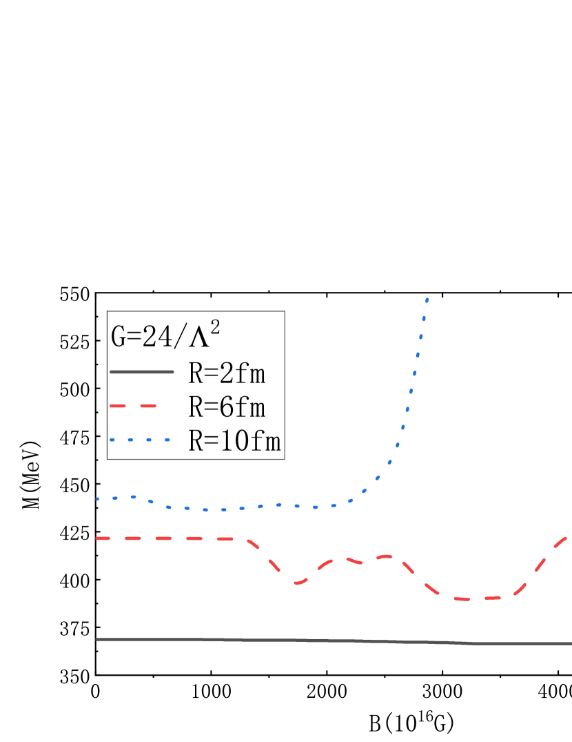
(a) $G=24/\Lambda^{2}$

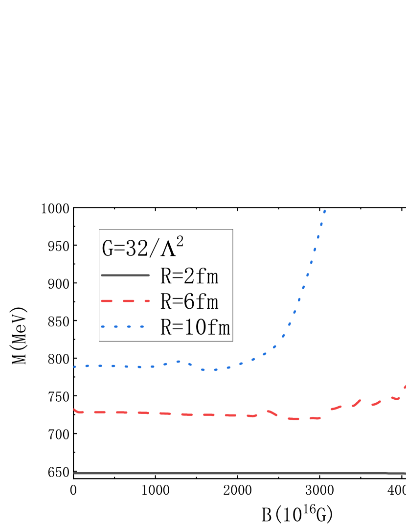
(b) $G=32/\Lambda^{2}$

Figure 1: Variation of the effective quark mass in a uniform magnetic field. The quarks are confined in a sphere with a radius of $R=2,6,10$ fm, respectively. Panels (a) and (b) correspond to $G=24/\Lambda^{2}$ and $G=32/\Lambda^{2}$, respectively.

The effects of a strong magnetic field on the effective quark mass for quarks confined in a sphere are illustrated in Fig. 1. We consider two different coupling constants, $G=24/\Lambda^{2}$ and $G=32/\Lambda^{2}$ in Fig. 1. In both cases, we see that the effective mass of quarks increases with the strength of the magnetic field when $R$ is large. This phenomenon is exactly the so called chiral magnetic catalysis. In general, such a chiral magnetic catalysis is also observed in the standard NJL model in an infinite space Gusynin et al. (1996); Andersen et al. (2016); Menezes et al. (2009). Moreover, when $R$ becomes small, the inverse magnetic catalysis is observed, i.e, the effective mass of quarks decreases with the increase of the magnetic field.

The influence of the radius, $R$, on the occurrence of magnetic catalysis or inverse magnetic catalysis can be observed more clearly in Fig. 2. Specifically, magnetic catalysis is observed at $R=5$ fm, inverse magnetic catalysis occurs at $R=3$ fm, and the case of $R=4$ fm falls between these two cases. It is well know that, at $T=0$, the standard NJL does not exhibit inverse magnetic catalysis. To explore the potential causes of the inverse magnetic catalysis here, we should return to Eq. (38) again. When $R$ is small, the contribution of the Lowest Orbital Level (LOL), i.e., $j=\frac{1}{2}$ and $\kappa>0$, reduces to

$$\langle\bar{\psi}\psi\rangle_{\text{main}}\xlongequal[\text{LOL}]{R\rightarrow 0}-\sum_{\lambda}w(E_{\lambda})\sum_{i}\frac{1}{V}|c_{i,n}|^{2}\frac{-E_{k}+2M}{-2E_{k}+M}.$$ (42)

Since $E_{k}=\sqrt{p_{j\kappa,i}^{2}+M^{2}}$, the contribution of these momentum modes to quark condensate will be positive for $p_{j\kappa,i}^{2}<\frac{M^{2}}{3}$, yielding an anomaly value. With the increase of the magnetic field, the energy gap between the orbital levels increases, causing the system to prefer the LOL and resulting in the inverse magnetic catalysis. Another factor is the intrinsic truncation caused by the small radius, which prevents the increase of Landau levels and the density of states. It further contributes to the inverse magnetic catalysis.

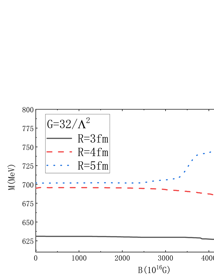
Figure 2: Variation of the effective quark mass in a uniform magnetic field near the critical radius for $G=32/\Lambda^{2}$.

Some oscillations could be seen in Fig. 1 when $R=6,10$ fm. They are quite similar to the de Haas-van Alphen oscillations Lifshitz and Pitaevskii (2013). Such an oscillation behavior could be caused by the variation of the density of states due to the Landau quantization, which has also been observed in the standard NJL model Chatterjee et al. (2011); Cao and Li (2023). On the other hand, when the radius is small, the intrinsic truncation imposes a cutoff on the Landau levels, suppressing the variation of the density of states. Consequently, the de Haas-van Alphen oscillations cease at small radii.

IV SUMMARY AND DISCUSSION

In this study, quark matter confined in a sphere with a strong uniform magnetic field is studied. The wave functions and energy levels are solved by diagonalizing the Hamiltonian numerically, using eigen solutions of Hamiltonian with a zero magnetic field as basis. The NJL model is employed, and by solving its gap equation, the inverse magnetic catalysis effect and magnetic catalysis effect is studied for a confined sphere with various radii. It is found that when the radius of the sphere is large, magnetic catalysis occurs, whereas when the radius is small, inverse magnetic catalysis occurs. At the intermediate region ($R\approx 4$ fm), both phenomena are present. It is argued that the inverse magnetic catalysis could be caused by the anomalous contribution from the LOL. Additionally, the intrinsic truncation due to small radius prevents the increase of Landau levels and density of states, which may also contribute to the inverse magnetic catalysis.

For simplicity, we mainly adopt the one-flavor NJL model with $q=1$ to investigate the chiral phase transition in our study. In fact, we have also performed calculations for the two-flavor NJL model, in which $q_{u}=\frac{2}{3}$ and $q_{d}=-\frac{1}{3}$. It is found that the results are generally similar. In the future, more realistic conditions should be considered. For example, the study of finite temperature effects and the impact of nonzero current quark mass in a two-flavor model might be of special interest, which could provide additional insights into the behavior of QCD fireballs produced in heavy-ion collisions under realistic conditions.

References

- Chernodub and Gongyo (2017) M. N. Chernodub and S. Gongyo, Phys. Rev. D 96, 096014 (2017).
- Chen et al. (2017) H.-L. Chen, K. Fukushima, X.-G. Huang, and K. Mameda, Phys. Rev. D 96, 054032 (2017).
- Sadooghi et al. (2021) N. Sadooghi, S. M. A. Tabatabaee Mehr, and F. Taghinavaz, Phys. Rev. D 104, 116022 (2021).
- Palhares et al. (2011) L. F. Palhares, E. S. Fraga, and T. Kodama, Journal of Physics G: Nuclear and Particle Physics 38, 085101 (2011).
- Klein (2017) B. Klein, Phys. Rept. 707-708, 1 (2017).
- Voronyuk et al. (2011) V. Voronyuk, V. D. Toneev, W. Cassing, E. L. Bratkovskaya, V. P. Konchakovski, and S. A. Voloshin, Phys. Rev. C 83, 054911 (2011).
- Deng and Huang (2012) W.-T. Deng and X.-G. Huang, Phys. Rev. C 85, 044907 (2012).
- Miransky and Shovkovy (2015) V. A. Miransky and I. A. Shovkovy, Physics Reports 576, 1 (2015).
- Gusynin et al. (1994) V. P. Gusynin, V. A. Miransky, and I. A. Shovkovy, Phys. Rev. Lett. 73, 3499 (1994).
- Ebert et al. (2000) D. Ebert, K. G. Klimenko, M. A. Vdovichenko, and A. S. Vshivtsev, Phys. Rev. D 61, 025005 (2000).
- Andersen et al. (2016) J. O. Andersen, W. R. Naylor, and A. Tranberg, Rev. Mod. Phys. 88, 025001 (2016).
- Bali et al. (2012a) G. S. Bali, F. Bruckmann, G. Endrodi, Z. Fodor, S. D. Katz, and A. Schafer, Phys. Rev. D 86, 071502 (2012a).
- Bali et al. (2012b) G. S. Bali, F. Bruckmann, G. Endrodi, Z. Fodor, S. D. Katz, S. Krieg, A. Schafer, and K. K. Szabo, JHEP 02, 044 (2012b).
- Bruckmann et al. (2013) F. Bruckmann, G. Endrodi, and T. G. Kovacs, JHEP 04, 112 (2013).
- Fraga et al. (2013) E. S. Fraga, J. Noronha, and L. F. Palhares, Phys. Rev. D 87, 114014 (2013).
- Ferrer et al. (2015) E. J. Ferrer, V. de la Incera, and X. J. Wen, Phys. Rev. D 91, 054006 (2015).
- Cao (2021) G. Cao, Eur. Phys. J. A 57, 264 (2021).
- Chen et al. (2016) H.-L. Chen, K. Fukushima, X.-G. Huang, and K. Mameda, Phys. Rev. D 93, 104052 (2016).
- Buballa (2005) M. Buballa, Phys. Rept. 407, 205 (2005).
- Chodos et al. (1974) A. Chodos, R. L. Jaffe, K. Johnson, C. B. Thorn, and V. F. Weisskopf, Phys. Rev. D 9, 3471 (1974).
- Rajaraman and Bell (1982) R. Rajaraman and J. S. Bell, Phys. Lett. B 116, 151 (1982).
- Zhang et al. (2020) Z. Zhang, C. Shi, X. Luo, and H.-S. Zong, Phys. Rev. D 102, 065002 (2020).
- Greiner et al. (2007) W. Greiner, D. Bromley, S. Schramm, and E. Stein, Quantum Chromodynamics (Springer Berlin Heidelberg, 2007).
- Wu and Wan (2012) S. Wu and L. Wan, Journal of Applied Physics 111 (2012), 10.1063/1.3695454.
- Cohen-Tannoudji et al. (1986) C. Cohen-Tannoudji, B. Diu, and F. Laloe, Quantum Mechanics 1, 898 (1986).
- Landau and Lifshitz (1999) L. D. Landau and E. M. Lifshitz, Statistical physics. Pt.1 (Statistical physics. Pt.1, 1999).
- Gusynin et al. (1996) V. Gusynin, V. Miransky, and I. Shovkovy, Nuclear Physics B 462, 249 (1996).
- Menezes et al. (2009) D. P. Menezes, M. Benghi Pinto, S. S. Avancini, A. Perez Martinez, and C. Providencia, Phys. Rev. C 79, 035807 (2009).
- Lifshitz and Pitaevskii (2013) E. M. Lifshitz and L. P. Pitaevskii, Statistical physics: theory of the condensed state, Vol. 9 (Elsevier, 2013).
- Chatterjee et al. (2011) B. Chatterjee, H. Mishra, and A. Mishra, Phys. Rev. D 84, 014016 (2011).
- Cao and Li (2023) G. Cao and J. Li, Phys. Rev. D 107, 094020 (2023).